Embed Size (px)
Citation preview

This thesis has been submitted in fulfilment of the requirements for a postgraduate degree
(e.g. PhD, MPhil, DClinPsychol) at the University of Edinburgh. Please note the following
terms and conditions of use:
This work is protected by copyright and other intellectual property rights, which are
retained by the thesis author, unless otherwise stated.
A copy can be downloaded for personal non-commercial research or study, without
prior permission or charge.
This thesis cannot be reproduced or quoted extensively from without first obtaining
permission in writing from the author.
The content must not be changed in any way or sold commercially in any format or
medium without the formal permission of the author.
When referring to this work, full bibliographic details including the author, title,
awarding institution and date of the thesis must be given.

The Impact of Fire on Blanket Bogs:
Implications for Vegetation and the Carbon Cycle
Emily Siobhan Taylor
Submitted for the degree of PhD
The University of Edinburgh
2014

i
Declaration of Authorship
I confirm that this work is my own and this thesis has been written by me unless
otherwise stated. No part of this work has been submitted for any other degree or
professional qualification.
Emily S Taylor
28th
September 2014

ii
Lay Summary
Peat is produced by the slow decomposition of plant material so is rich in
carbon. In the UK peat soils are a bigger carbon store than all the vegetation growing
above ground making them very important in the context of carbon cycling and
greenhouse gas emissions from land use and climate change. Blanket bogs are a
special type of peatland, with deep peat soils and waterlogged conditions, globally
recognised for their carbon storage capacity and their wildlife. In the UK they are
also important to a number of industries and managed for forestry, farming and game
such as red grouse and deer. Fire has been used by land managers for over a century
as a way of improving grazing and habitat for livestock and game and, although of
concern, the impacts of burning on the ecology and carbon cycle of blanket bogs is
relatively understudied. The objective of this research was to assess the effect of fire
on Sphagnum, important bog mosses, and greenhouse gas emissions from blanket
bogs.
Methane emissions and the release of carbon dioxide by plants and bacteria
(respiration) were measured at three sites in Scotland which had recently been burnt.
The response of Sphagnum to different fire conditions was also assessed at the field
sites and in a unique laboratory experiment. The effect of fire on methanotrophic
bacteria, bacteria which use methane as food turning it into carbon dioxide and found
in Sphagnum, was studied in the laboratory to see if the high temperatures caused by
fire would kill the bacteria and thus, be a mechanism for fire increasing methane
emissions to the atmosphere. The results show that fire did not increase methane
emissions or respiration over the study period and that Sphagnum had the capacity to
respond to fire by growing new stems. Methane removal by bacteria in samples of
Sphagnum was found to be difficult to detect, with no affect of fire observed. Despite
these results suggesting that low severity fires, which leave the moss layer and peat
intact, have no impact on the elements of the carbon cycle studied here and can be
survived by Sphagnum, they reiterate that burning legislation and guidelines must
continue to strive to ensure that burning is only carried out on blanket bogs when
conditions are conducive to low severity fires.

iii
Abstract
Peatlands are multiservice ecosystems: they are the largest terrestrial store of
carbon in the UK, unique habitats which provide a home for internationally
important species and managed for forestry, farming and game management and
shooting. This makes understanding the impact of management practices on their
ecology important if they are to be sustainably managed for multi-benefits. Fire has
long been used to manage peatlands in the UK to improve grazing and habitat
provision for livestock and game. The effect of fire on carbon cycling in blanket bogs
is of increasing concern as greenhouse gas emissions from land use is now an
important management as well as political issue. Gaps however, still exist in our
understanding of the controls on greenhouse emissions from blanket bogs and the
impact fire may have on them both directly and indirectly by modifying vegetation
composition and environmental conditions.
The main objective of this research was to assess the effect of fire on
greenhouse gas emissions by measuring methane and ecosystem respiration after
burning at blanket bog sites across Scotland for a period of up to 3 years and relating
changes in fluxes with changes in vegetation composition and abiotic conditions. In
addition, the response of the Sphagnum layer to burning was assessed by looking at
the recovery of Sphagnum capillifolium in the field and in a novel laboratory
experiment. The indirect effects of fire on methane emissions were further
investigated by a laboratory experiment devised to test if high temperatures would be
fatal to methanotrophic bacteria in the Sphagnum layer, reducing methanotrophy, and
thus a mechanism for fire to increase methane emissions in the short term.
The results showed that methane emissions and ecosystem respiration were
not significantly different in burnt plots when compared to adjacent unburnt plots at
each of the three sites studies. Methane emissions were only weakly correlated to the
position of the water table and neither methane fluxes or ecosystem respiration
correlated with measures of vegetation composition and above ground biomass.
Methanotrophy in Sphagnum was found to be difficult to detect, with a high
temperature treatment having no significant effect on rates of methane oxidation.
iv
S. capillifolium was found to respond to fire by growing new auxiliary stems if the
capitulum was consumed or irreversible damaged physiologically by temperatures
experienced at the moss surface, with surface temperatures around 400oC with a
temperature residency time of 30 seconds on artificially dried samples the most
damaging, but not lethal, treatment.
These results suggest that low severity fires which only consume the canopy
vegetation, not penetrating the peat and leaving the moss layer mostly intact, do not
have significant effects on methane emissions and ecosystem respiration in the short
and medium term. In addition, it suggests that S.capillifolium can, under certain
circumstances, survive a fire with the characteristics of those studied here. These
findings reiterate that best practice burning guidelines must continue to ensure that
burning is only carried out on blanket bog when conditions are conducive to fires
with the characteristics studied here, which had little effect on important components
of the carbon cycle and are survivable by at least one of the most common species of
Sphagnum.

v
Acknowledgements
I have many people to thank for the journey to, and the journey through, my
PhD, and I hope that I can go some way here to express my sincere thanks to you all.
Thanks go firstly to the many organisations which funded and supported this
research: Scottish Natural Heritage (SNH) and the Scottish Environment Protection
Agency (SEPA) through their jointly funded PhD studentship scheme, the Royal
Society for the Protection of Birds (RSPB) and the Centre for Ecology and
Hydrology (CEH) for additional funding for field work and equipment. Secondly,
thanks to my supervisors from these organisations: Graham Sullivan (SNH), Neil
Cowie (RSPB), Janet Moxley and Lorna Harris (SEPA). Thanks also to Colin Legg
for his initial input into the project, and Mathew Williams at the University of
Edinburgh for support throughout. Special thanks, however, go to my two CEH
based supervisors, Peter Levy and Alan Gray, for coming together and combining
their expertise to support, advise and help me out throughout the four years of this
PhD. I have very much enjoyed working with you both and want to express my
gratitude for all the time you have spent with me on this project, not to mention
ensuring no (or only some) equipment was burned in the name of science.
I could not have done any of my field work without the permission of the
land owners and managers who so kindly allowed me onto their land. Massive thanks
to Ali and Susan Cowan at Eastside, I am enormously grateful to you for letting me
onto your farm with my orange wheel barrow and strange equipment. To Neil Cowie
and Norrie Russell at Forsinard for allowing me to set up on the reserve, and all the
advice and information you gave me (thanks must also go to that train...). Finally to
Debbie Fielding at the James Hutton Institute who helped me out with Glensaugh.
There have been many others who have helped me along the way, thank you
to you all but a special mention must go to: Fraser Leith, for 4x4 support, not letting
me forget about DOC and general PhD and peatland discussions, Lucy Shepherd for
her help with, and enthusiasm for, all things Sphagnum, Julia Drewer for continued

vi
GC support, Matt Davies for temperature data and guidance in the early stages, and
all those who have helped me with field work. Thanks also to my colleagues at the
Crichton Carbon Centre for being so supportive in these final months.
Finally I could not have got through it all, or even contemplated embarking
on a PhD, without the unwavering support of friends and family. Special thanks to
my Granny and Grandad who have helped so much with my education and who have
always been so proud and supportive. An enormous thank you to my Mum and Dad
for everything, but most of all instilling in me my love of the countryside and the
peat bogs which I am now so fortunate to make my professional career. Lastly, thank
you Jamie, I am so grateful for you always being there to tell me “everything will be
fine”.

vii
Dedication
To my Grandad
Douglas Ward Beasley
1925-2014

viii
Contents
Declaration of Authorship ........................................................................................ i
Lay Summary .......................................................................................................... ii
Abstract .................................................................................................................. iii
Acknowledgements ................................................................................................. v
Dedication ............................................................................................................ viii
1. Introduction ............................................................................................................ 1
1.1 Peatlands: Globally Important Ecosystems ........................................................ 1
1.2 Fire in Northern Peatlands .................................................................................. 2
1.3 Peatland in the UK ............................................................................................. 4
1.4 Fire in the UK ..................................................................................................... 6
1.5 Characteristics of Prescribed Fires ................................................................... 10
1.6 Aims of this Research ...................................................................................... 12
1.7 References ........................................................................................................ 14
2. The Impact of Burning on CH4 Fluxes and Ecosystem Respiration of Blanket
Bogs ........................................................................................................................... 20
2.1 Abstract ............................................................................................................ 20
2.2 Introduction ...................................................................................................... 21
2.2.1 Fire and the Peatland Carbon Cycle ...................................................... 21
2.3 Aims ................................................................................................................. 27
2.4 Methodology .................................................................................................... 28
2.4.1 Site descriptions ..................................................................................... 28
2.4.2 Sampling Methodology.......................................................................... 31 2.4.3 Gas Chromatography ............................................................................. 33 2.4.4 Flux Calculations ................................................................................... 34 2.4.5 Vegetation Assessment .......................................................................... 35 2.4.6 Statistical Analysis ................................................................................. 36
2.5 Results .............................................................................................................. 37
2.5.1 Soil Moisture, Water table and Soil Temperature ................................. 37
2.5.2 CH4 Fluxes ............................................................................................. 38 2.5.3 Ecosystem Respiration ........................................................................... 41 2.5.4 Fluxes and Vegetation ........................................................................... 44

ix
2.6 Discussion ........................................................................................................ 47
2.6.1 CH4 fluxes ............................................................................................. 47 2.6.2 Ecosystem Respiration ........................................................................... 50
2.7 Conclusions ...................................................................................................... 52
2.8 References ........................................................................................................ 54
Appendix 2.1. Field Sites: Maps, Photographs and Sampling Times ................... 61
Appendix 2.2. Soil Temperature, Soil Moisture and Water table at the three field
sites ......................................................................................................................... 68
Appendix 2.3. Methane fluxes at each site at each sampling time ........................ 72
Appendix 2.4. Ecosystem Respiration at each site at each sampling time ............ 74
3. The recovery of Sphagnum capillifolium following exposure to temperatures
of simulated moorland fires: a glasshouse experiment ......................................... 75
3.1 Abstract ............................................................................................................ 75
3.2 Introduction ...................................................................................................... 76
3.3 Aims ................................................................................................................. 81
3.4 Materials and Methods ..................................................................................... 81
3.4.1 Experimental Design.............................................................................. 81 3.4.2 Recovery Measurements ........................................................................ 86 3.4.2.1 Chlorophyll Fluorescence .......................................................... 86
3.4.2.2 CO2 Exchange ............................................................................ 87 3.4.2.3 New Growth and Physical Damage ........................................... 90
3.4.3 Statistical Analysis ................................................................................. 91
3.5 Results .............................................................................................................. 93
3.5.1 Physical Damage.................................................................................... 93 3.5.2 Chlorophyll florescence ......................................................................... 96 3.5.3 CO2 Exchange ........................................................................................ 99
3.5.4 New Growth ......................................................................................... 104
3.6 Discussion ...................................................................................................... 106
3.6.1 Photosynthetic Capacity and CO2 Exchange ....................................... 106 3.6.2 New Growth ......................................................................................... 112
3.7 Conclusions .................................................................................................... 115
3.8 References ...................................................................................................... 117
Appendix 3.1 Glasshouse Watering Trial ............................................................ 122
Appendix 3.2 Schematic of experimental design and sampling procedure ......... 123

x
Appendix 3.3 Maximum temperatures and temperature residency time of each
treatment ............................................................................................................... 124
Appendix 3.4 Glasshouse conditions ................................................................... 126
Appendix 3.5 Rates of Photosynthesis in Sphagnum capillifolium at different light
intensities using Licor Li-6400 and specifically designed sample chamber ........ 129
Appendix 3.6 Bleaching evident prior to burning, 1 day after burning and 4 days
after burning in Run 2 of the experiment. Yellow circles highlight pots which
showed a delay in bleaching ................................................................................. 130
Appendix 3.7. Photographs of new auxiliary stem growth observed 100 days after
burning in runs 1 and 2 of the experiment ........................................................... 131
4. Methanotrophy in Sphagnum and the potential impact of fire...................... 133
4.1 Abstract .......................................................................................................... 133
4.2 Introduction .................................................................................................... 134
4.3 Aims ............................................................................................................... 136
4.4 Methodology .................................................................................................. 137
4.4.1 Sampling Site ....................................................................................... 137
4.4.2 Experimental Methodology ................................................................. 137 4.4.3 Verification of methodology ................................................................ 140 4.4.4 Calculating concentrations and oxidation rates ................................... 141
4.4.5 Statistical Analysis ............................................................................... 142
4.5 Results ............................................................................................................ 142
4.5.1 CH4 Oxidation...................................................................................... 142
4.5.2 CO2 fluxes ............................................................................................ 149
4.6 Discussion ...................................................................................................... 151
4.6.1 Experimental Error .............................................................................. 151 4.6.2 CH4 Oxidation...................................................................................... 153
4.7 Conclusions and Future Research .................................................................. 156
4.8 References ...................................................................................................... 158
Appendix 4.1. Concentrations of CH4 and CO2 ................................................... 162
5. The impact of burning on vegetation of three blanket bogs in Scotland ...... 165
5.1 Abstract .......................................................................................................... 165
5.2 Introduction .................................................................................................... 166
5.3 Aims ............................................................................................................... 168

xi
5.4 Methodology .................................................................................................. 170
5.4.1 Site description and survey methodology ............................................ 170 5.4.2 Percentage top cover assessment ......................................................... 171 5.4.3 Total percentage cover and dry weight ................................................ 173
5.4.4 Assessment of Sphagnum recovery ..................................................... 174 5.4.5 Statistical Analysis ............................................................................... 176 5.4.5.1 Analysis I ................................................................................. 176 5.4.5.2 Analysis II ................................................................................ 177 5.4.5.3 Recovery of Sphagnum capillifolium ...................................... 178
5.5 Results ............................................................................................................ 178
5.5.1 Change in vegetation following fire .................................................... 178 5.5.1.1 Analysis I ................................................................................. 178 5.5.1.2 Analysis II ................................................................................ 181 5.5.1.3 NVC Classifications ................................................................ 187
5.5.2 Recovery of S.capillifolium ................................................................. 191
5.6 Discussion ...................................................................................................... 196
5.6.1 Changes in vegetation composition ..................................................... 196
5.6.2 NVC Classifications ............................................................................ 199 5.6.3 Sphagnum Survival and Recovery ....................................................... 202
5.7 Conclusions .................................................................................................... 202
5.8 References ...................................................................................................... 204
Appendix 5.1 Species lists and comparison of top and full cover vegetation
surveys .................................................................................................................. 208
Appendix 5.2 Full species names and species author .......................................... 211
Appendix 5.3 Images of Sphagnum damaged by fire .......................................... 212
6. Synthesis ............................................................................................................ 214
6.1 The impact of burning on greenhouse gas emissions from blanket bogs ....... 215
6.2 The Impacts of burning on Sphagnum ........................................................... 220
6.3 Conclusions and Implications for Management in the UK ............................ 226
6.4 References ...................................................................................................... 228
xii
List of Figures
Figure 2. 1 The mechanisms for surface exchange of CO2 and CH4 in a
peatland system. .................................................................................... 24
Figure 2. 2 CH4 fluxes at each site (E=Eastside, G=Glensaugh, F=Forsinard)
under each treatment ............................................................................. 39
Figure 2. 3 The amount of within treatment variance explained by the
different random effects terms in the largest CH4 mixed effect
model described in Table 2. 5.. ............................................................. 40
Figure 2. 4 Ecosystem Respiration (ER) at each site (E=Eastside,
G=Glensaugh, F=Forsinard) under each treatment............................... 42
Figure 2. 5 The amount of within treatment variance explained by the
different random effects terms in the largest ER mixed effect
model described in Table 2. 7. .............................................................. 43
Figure 2. 6 Methane fluxes at each plot plotted against (a) total vascular plant
biomass, (b) total vascular plant leaf area, (c) total percent
Sphagnum spp. cover and (d) total Eriophorum spp. dry weight. ........ 45
Figure 2. 7 Ecosystem Respiration (ER) at each plot plotted against (a) total
vascular plant biomass, (b) total vascular plant leaf area, (c) total
percent Sphagnum spp. cover and (d) total Eriophorum spp. dry
weight.. .................................................................................................. 46
Figure 3. 1 Mean depth ± SEM of bleaching in a sub-sample of pots from
runs 2 and 3 (n= 6 stems per pot, 16 pots per treatment, per run).
No permanent bleaching was recorded in any control pots. All
pots harvested on day 100. Means with different letters are
significantly different (Welch Two Sample t test: t=-4.6, df=39.6,
p=<0.05 and t=-5.1, df=25.1, p=<0.05 respectively). ........................... 94
Figure 3. 2 Fv/Fm ratio of 5mm sections of stem starting from the capitulum
(position 0mm) from a sub-sample of pots exposed to the three
treatment in Run2 of the experiment (n=6 per treatment). Plots
fitted with locally estimated scatterplot smoothing (LOESS)
regression lines (fitted over all points by weighted least squares
with a smoother span of 0.75). .............................................................. 95
Figure 3. 3 The number of stems showing capitulum decay, defined as the
distance from the capitulum down the stem showing bleaching
and/or reduced structural integrity, at each sampling time for each
treatment during runs 2 and 3 of the experiment (n=8 stems per
treatment per sampling time per run). No capitulum decay
occurred in control pots. ....................................................................... 96
xiii
Figure 3. 4 Fv/Fm ratio of stems taken from pots subjected to each treatment
over the three runs, Spring, Autumn and Winter of the experiment
(n=8 per treatment per sampling time). Points show mean Fv/Fm
±SEM bars fitted with LOESS regression lines (parameters as in
Figure 3. 2). ........................................................................................... 97
Figure 3. 5 Amount of within treatment variance explained by the different
random effects terms in the largest mixed effect model described
in Table 3.3.. ......................................................................................... 98
Figure 3. 6 The rate of photosynthesis (RoP) of pots in each treatment group
during each run when PAR=2000 µmol m2 s
-1. Points show mean
±SEM bars fitted with LOESS regression line (parameters as in
Figure 3. 2). ......................................................................................... 100
Figure 3. 7 The rate of respiration of pots in each treatment group in runs 2
and 3 of the experiment measured when PAR = <1 µmol m2 s
-1. ...... 101
Figure 3. 8 Amount of within treatment variance explained by the different
random effects terms in the largest mixed effect model described
in Table 3. 4. ....................................................................................... 102
Figure 3. 9 Amount of within treatment variance explained by the random
effects terms in the largest mixed effect model described in Table
3. 5. ..................................................................................................... 103
Figure 3. 10 New growth (measured as biomass dry weight) shown as a ratio
to total original sample biomass dry weight for each treatment and
run of the experiment. ......................................................................... 104
Figure 3. 11 The location of new growth found in a subsample of 16 pots per
treatment per run showing (a) the total number of new side and
base innovations seen in runs 2 and 3 and (b) the mean location of
new auxiliary side innovations in relation to the mean depth of
bleaching in the same pot shown with StE bars. ................................. 105
Figure 4. 1 Experimental set up showing jars filled with Sphagnum samples
and the valve mechanism and syringes used to remove headspace
gas samples. ........................................................................................ 138
Figure 4. 2 CH4 fluxes for each treatment (UB=unburnt, B=burnt, E=empty)
per run of the experiment. Solid vertical lines show the median,
boxes the lower and upper quartiles, whiskers the extent of upper
and lower values within 1.5*inter quartile range and points
outliers.. .............................................................................................. 144
Figure 4. 3 CH4 (a) and CO2 (b) fluxes in relation to sampling location used
in Runs 4 and 5 where S.capillifolium was sampled from 10
hummocks in Run 4 and S.papillosum taken from 4 lawns in Run
5.. ........................................................................................................ 146
xiv
Figure 4. 4 Conditional kernel density plot of CH4 fluxes observed in
Sphagnum free jars with (n=11) and without (n=23) the addition
of mixers where dashed lines represent means. .................................. 147
Figure 4. 5 Boxplots (left) and conditional kernel density plots (right) of CH4
fluxes calculated per jar per day for each temperature treatment
compared to (a) all Sphagnum-free jars and (b) only those
Sphagnum-free jars containing mixers (B are burnt, UB unburnt
and E Sphagnum free jars).. ................................................................ 148
Figure 4. 6 CO2 concentrations over time for each treatment (B=Burnt,
UB=Unburnt, E=Sphagnum-free jars) with regression lines for
each. Burnt Sphagnum jars had a mean flux of 207.6±SE15.1
µmol CO2 jar-1
day-1
, unburnt Sphagnum jars had a mean flux of
202.1±SE14.5 µmol CO2 jar-1
day-1
, and Sphagnum free jars had a
mean flux of -0.2±SE0.2 µmol CO2 jar-1
day-1
. .................................. 149
Figure 4. 7 CO2 fluxes for each species where Scap=S.capillifolium,
Sfal=S.fallax, Spap=S.papillosum, n=40, 19, 20 respectively.
indicates significant difference between adjacent species, where
(sqrt transformed) t=-6.9, df=53, p=<0.001. ....................................... 150
Figure 4. 8 CO2 fluxes in relation to Sphagnum dry weight with linear
regression lines for each sample by species where
Scap=S.capillifolium, Sfal=S.fallax, Spap=S.papillosum. .................. 150
Figure 5. 1 Example image of a plot where percentage top cover of each plant
species was surveyed, showing the superimposed digital 8-sector
layer to aid assessment. ....................................................................... 173
Figure 5. 2 DCA ordination diagram with (a) species composition assessed
by total percent cover on final day of sampling plotted with site
(G=Glensuagh, E=Eastside, F=Forsinard), where empty triangles
denote species and large filled triangles denote site and (b) a
projection of the environmental variables; site, altitude, aspect,
slope, cardinal and intercardinal direction (Easting/Northing),
precipitation (Precipit), water table (WT), mean soil temperature
(ST_M) and soil moisture (SM), onto the species data.. .................... 180
Figure 5. 3 Principal Response Curve of Forsinard vegetation at the three
sampling times where burnt plots were compared to unburnt
control plots and individual species scores (full species names
given in Appendix 5.2) for Axis 1 (a), (b). The effect of treatment
and it’s interaction with timepoint according to Monte Carlo
permutation test was not significant (p=0.148). ................................. 183
Figure 5. 4 (a) Principal Response Curve of Eastside vegetation at the three
sampling times where burnt plots were compared to unburnt
control plots and (b) individual species scores (full species names
given in Appendix 5.2).The effect of treatment and it’s interaction

xv
with timepoint according to Monte Carlo permutation test was
significant (p=0.01). ............................................................................ 184
Figure 5. 5 (a) Principal Response Curve of Glensaugh vegetation at the three
sampling times where burnt plots were compared to unburnt
control plots. The effect of treatment and it’s interaction with
timepoint according to Monte Carlo permutation test was not
significant (p=0.258) and (b) individual species scores. Full
species names given in Appendix 5.2. ................................................ 185
Figure 5. 6 Difference in percentage cover of shrubs (a) and graminoids (b) at
each site at each sampling time in the burnt and unburnt plots
(calculated as Burnt minus Unburnt percentage cover) where
minus values represent a lower cover in the burnt plots when
compared to unburnt plots. The shrub group consisted Calluna
vulgaris (dominant), Vaccinium myrtillus, Myrica gale and Erica
tetralix. The graminoid group was made up of Eriophorum
vaginatum (dominant), Eriophorum angustifolium and
Deschampsia flexuosa. ........................................................................ 186
Figure 5. 7 NVC sub-communities matched to the vegetation at each site over
time and treatments using top cover survey method.. ......................... 190
Figure 5. 8 Fv/Fm of the capitula of S.capillifolium at each site in the days
after the site was subjected to burning where dark grey bars are
burnt samples and light grey unburnt. ................................................ 192
Figure 5. 9 Stem moisture content of a sample of S.capillifolium removed
from each hummock plotted with mean Fv/Fm (±StE bars) of the
capitula of and (b) mean (±StE bars) stem moisture content of
burnt and unburnt samples at each site and sampling day where
recovery day was the number of says since sites were burned. .......... 193
Figure 5. 10 Mean (±StE bars) Fv/Fm of the capitula of S.capillifolium at
Eastside which had been burned 184 days previously (Burnt),
compared to unburnt hummocks (Unburnt) and new auxiliary
capitula (New) found growing on stems in hummocks which had
been damaged by the fire (see Figure 5. 12). The results of a
Kruskal–Wallis test were significant (df=2, p=<0.001). ................... 194
Figure 5. 11 New auxiliary growth observed on S.capillifolium stems that had
been subjected to burning at Eastside (photograph taken 184 days
after the fire had occurred). The same auxiliary growth was seen
at all three sites. .................................................................................. 195
Figure 5. 12 A hummock of S.capillifolium at Forsinard which had been burnt
428 days previously showing the new auxiliary growth which
appear as red capitula surrounded by bleached material (the
remainder of the original stem) (enlarged in inset) ............................. 195

xvi
List of Tables
Table 1. 1 Summary of key management restrictions and guidance for
prescribed burning in Scotland and England set out in the
Muirburn Code (Scotland) and the Heather and Grass Burning
Code (England). ...................................................................................... 9
Table 2. 1 Gas sampling site descriptions (See Appendix 2.1for maps and
images) .................................................................................................. 30
Table 2. 2 Dry weights of the most significant components of the vegetation
from harvested plots adjacent to burned areas at Forsinard and
Eastside as an indication of differences in fuel load and structure.
Weights given are summed from 6 randomly sampled plots at
each site covering a total area 0.9 m2. For full details of the
species making up each component see Chapter 5. .............................. 31
Table 2. 3 Fixed and random effects terms used in mixed effects modelling
of CH4 fluxes and ecosystem respiration (ER). .................................... 37
Table 2. 4 CH4 fluxes at each site and treatment (µmol m2 s
-1) ............................. 39
Table 2. 5 Results of linear mixed effects model of CH4 fluxes with the
optimum model selected using AIC criteria to determine random
and fixed effects. Model with the lowest AIC criteria and thus
largest negative delta AIC (∆AIC) was selected. ................................. 40
Table 2. 6 ER at each site and treatment (µmol m2 s
-1) ......................................... 41
Table 2. 7 Results of linear mixed effects model of ER with the optimum
model selected using AIC criteria to determine random and fixed
effects. Models with the lowest AIC criteria and thus largest
negative delta AIC (∆AIC) were selected. ............................................ 43
Table 3. 1 Temperature treatments used for each of the three runs of the
experiment. ........................................................................................... 84
Table 3. 2 Fixed and random effects terms used in mixed effects modelling
of the repeated measures of chlorophyll fluorescence and CO2
exchange.*Moisture content term only used in chlorophyll
fluorescence model as stems were harvested for moisture content
analysis only on days fluorescence measurements were made. ............ 92
Table 3. 3 Results of linear mixed effects model of the Fv/Fm ratio
(transformed using Arc Sine transformation) with appropriate
model selected using AIC criteria to determine random and fixed
effects and a Wald test for fixed term significance. Models with
the lowest AIC criteria and thus largest negative delta AIC
(∆AIC) were selected. MC = moisture content of Sphagnum stems
at time of measurement. ........................................................................ 98

xvii
Table 3. 4 Results of linear mixed effects model of the rate of photosynthesis
(µmol CO2 g[dry weight]-1
day-1
) with smallest model with the
lowest AIC shown in bold. ................................................................. 102
Table 3. 5 Results of linear mixed effects model of the respiration rate (µmol
CO2 g[dry weight]-1
day-1
). The most appropriate model with
lowest AIC shown in bold. Random effects calculated using
REML estimates and fixed effects using ML estimates. .................... 103
Table 4. 1 Sampling methodology for each run of experiment (species are
S.cap=S.capillifolium, S.fal=S.fallax, S.pap=S.papillosum), the
date of each run and mean moisture content (MC) of samples
calculated on a percentage wet weight basis. ..................................... 140
Table 4. 2 Results of One-Way ANOVA tests between all three treatments
for each run of the experiment where burnt (B) and unburnt (UB)
Sphagnum-filled jars were compared to all empty (E) jars
analysed across the 5 runs of the experiment. Significant
differences between groups shown in bold. ........................................ 145
Table 5. 1 Vegetation survey site descriptions (See Appendix 2.1 for maps
and images of the sites). M
measured, 1Levy et al. (2012),
2Centre
for Ecology and Hydrology (2012), 3Ball et al. (2012) ,
4UK
Environmental Change Network (2012). ............................................ 172
Table 5. 2 Sampling procedure for chlorophyll fluorescence measurements
at each field site where S.capillifolium was sampled from
hummocks or areas of lawn at various time points after the site
was burnt. ............................................................................................ 176
Table 5. 3 Summary of DCA ordination analysis for Analysis I (total %
cover of each species on final day of sampling) showing
eigenvalues, which indicate high variation within the data, and the
proportion of cumulative variation explained by axis 1 and 2.
Supplementary variables accounted for 25.6% (adjusted explained
variation 14.9%) .................................................................................. 179
Table 5. 4 The amount of total and partial variance explained by Treatment
and Time for each site and the significance of Axis 1 (significant
result shown in italics) ........................................................................ 182
Table 5. 5 NVC sub communities matched to burnt and unburnt control
community at each site and sampling time (T1, T2, T3) showing
the number of species in each community and match statistics. ........ 188

Chapter 1. Introduction 1
1. Introduction
1.1 Peatlands: Globally Important Ecosystems
Peatlands can be found across the world and cover around 3.8 million km2,
3% of the earth’s surface (Joosten, 2010). The term peatland describes systems
where the accumulation of peat, formed from organic matter due to slow rates of
decay, is the common feature. Most peatlands are found in the cold boreal and sub-
arctic regions or in the tropics where the cold or wet and humid climates facilitate
anoxic conditions and slow rates of decay (Parish et al., 2008). Peatlands can be
divided into four main ecosystems; marshes, which are permanently flooded,
swamps, characterised by a lower water table, fens which are minerotrophic with a
water table close to the surface, and bogs which also have a water table close to the
surface but receive their nutrients and water solely from precipitation, making them
ombrotrophic (Rydin and Jeglum, 2006). These unique conditions not only vary
between these ecosystems but also considerably within a system. In bogs areas can
be characterised as lawns, pools, hollows and hummocks depending on Sphagnum
moss growth and moisture regimes, all of which support unique assemblages of
organisms adapted to life in the different conditions. Traditionally the importance of
peatlands has been valued in relation to the unique habitats they provide and the
specialised organisms they support, but increasingly their global significance is
emphasised in relation to their role in the terrestrial carbon cycle.
Acting as a long term carbon sink, it is estimated that peatlands store 30% of
the world’s soil carbon (Parish et al., 2008) and so within the context of greenhouse
Chapter 1. Introduction 2
gas emissions and climate change they act to sequester CO2 and lock away carbon
from the atmosphere. The observed rise in the atmospheric concentrations of
greenhouse gases such as CO2 and CH4, both gases naturally emitted from peatlands,
is now understood to drive global warming and changes in our climate (IPCC, 2013).
This makes managing peatlands to help mitigate climate change of higher priority
politically and has given rise to international incentives to promote the restoration
and sustainable management of peatlands through initiatives such as the Clean
Development Mechanism under the Kyoto Protocol and Nationally Appropriate
Mitigation Actions (NAMAs) aimed at developing countries (FAO and Wetlands
International, 2012) and more locally the Peatland Action fund for peatland
restoration in Scotland. However, peatlands are valued as “multi-service” ecosystems
and are managed across the world for agriculture and forestry and provide a host of
other services such as water regulation and nutrient cycling (Millenium Ecosystem
Assessment, 2005). Conflict inevitably arises between different management
objectives and utilisation of services, with management practices having the potential
to be detrimental to the ecology of a peatland. Understanding the full impacts of
management practices and disturbance events on a peatland system is therefore
important in informing sustainable management and ensuring peatlands still provide
their vital services.
1.2 Fire in Northern Peatlands
Fire, a naturally occurring form of disturbance caused by lightning strikes,
can affect extensive areas of a peatland and evidence suggests that the frequency and
severity of fires in the future will increase with global warming (Schneider et al.,

Chapter 1. Introduction 3
2007). Fires are also started deliberately, used as a management tool to regenerate
vegetation and clear land for farming and forestry. This makes fire important to
understand if we are to mitigate the risk of both wild and management fires which
are detrimental to the ecology and carbon cycle of a system.
Fires regularly occur on open and forested peatlands across the world (NASA
Earth Observations, 2014). Russia, which has the greatest peatland cover of any
country, and the second largest peat carbon stock after Canada (Joosten, 2010), has
seen significant wildfires in recent years. One estimate suggests that 8.23 million ha
(±9%) burns annually in the territories of Russia (Shvidenko et al., 2011). In Canada
it is estimated that an average 9000 fires occur annually which can burn up to 2
million ha (Natural Resources Canada, 2012) and in Alaska 613 fires occurred in
2013 alone, covering an area over 500,000 ha (Alaska Interagency Coordination
Centre, 2013). Fires can vary not only in their geographical extent but also their
severity, which is usually defined by how much organic matter gets consumed during
a fire (Keeley, 2009). Of concern is the growing evidence that climate change and
the associated increases in air temperatures and changes in precipitation patterns is
driving an increase in both fire frequency and severity (Gillett et al., 2004). North
America for example is now seeing double the number of peatland fires than it did in
the 1950’s, which is linked to a lower watertable and associated drying (Kasischke
and Turetsky, 2006).
Chapter 1. Introduction 4
1.3 Peatland in the UK
Under the UK soil classification system peatland soils can be classed as soils
with peaty pockets, shallow peat soils and deeper peaty soils with a peat depth
greater than 50cm and include fens, blanket bog and raised bogs, the majority being
blanket bog (Joint Nature Conservation Committee, 2011). Although in global terms
the UK holds less than 0.5% of the global peatland area (Joosten, 2010), at the
country scale around one third of the UK is covered by peat soils, the vast majority
found in Scotland (JNCC 2011). This makes it a substantial part of the UK’s land
resource and significant carbon store, estimated to contain 3000 Mt of carbon (Smith
et al., 2007). Peatlands are however, also valued for their habitat and the species
assemblages which they support.
Under the EC Habitats Directive many peatland habitats types are Annex 1
Habitats and in the UK are recognised as Biodiversity Action Plan Priority Habitats
with many designated Sites of Special Scientific Interest or Specials Areas of
Conservation for their fauna and flora. They support, although often not exclusively,
species of conservation concern, designated both in the UK and internationally (Joint
Nature Conservation Committee, 2014) and internationally blanket bogs are
particularly recognised for their breeding bird assemblage (Littlewood et al., 2010).
Although species are not always exclusive to certain peatland habitats they are often
highly specialised for living in the wet and acidic conditions. Species groups may be
particularly important for ecosystem functions, such as the peat forming Sphagnum
mosses and invertebrate and bacterial groups associated with the processing of plant
litter in the decay process (Coulson and Butterfield, 1978). Populations of grazing

Chapter 1. Introduction 5
mammals supported by peatlands such as red deer (Cervus elaphus) and ferral goats
may also have important implications for vegetation and peatland condition (LINK
Deer Task Force, 2013). Most peatlands in the UK have, however, been modified in
some way by man, with significant areas of blanket, basin and lowland peats eroded,
drained and managed for agriculture and forestry (Joint Nature Conservation
Committee, 2011).
Peatlands in the UK are important for farming and game management which,
particularly in the last 100 years, has led to the extensive drainage of both upland
blanket bog and lowland raised bog to improve grazing. Drains are cut to lower the
water table, which can have pronounced long term effects on the hydrology over
large areas and subsequently vegetation composition, biodiversity and carbon
cycling. Lowering the water table will cause the upper layers of peat to dry out,
increasing oxidation of the peat and carbon loss (Bussell et al., 2010). Drains can
also directly export carbon from a system as dissolved and particulate carbon as well
as cause significant erosion of the peat mass (Holden et al., 2004). Peat forming
function may also be lost due to drier conditions and a reduction in peat forming
species such as the Sphagnum mosses (Lindsay, 2010). In recent years this had lead
to funding being made available through agri-environment schemes and Government
funded initiatives, such as the Peatland Action fund in Scotland (Scottish Natural
Heritage, 2015), to block drains and increase the height of the water table to improve
conditions for peat formation, reduce carbon loss and improve bog habitat. Peatlands
are also drained and ploughed for commercial forestry which can have long term
implications for their ecology (Lindsay et al., 2014a). Lowland raised bogs in
Chapter 1. Introduction 6
particular have also been extensively drained for agriculture, forestry and
commercial extraction for peat for the horticulture industry. In England for example
two fifths of raised bogs have been reclaimed for agriculture, with another sixth
under forestry (Joint Nature Conservation Committee, 2011). Peat has also been cut
commercially for use as a fuel and domestic peat cutting has long been vital to areas
where wood fuel was not available such as the Shetland and Western Isles (Lindsay
et al., 2014b). The less direct impacts of grazing, burning and pollution from sulphur
dioxide from fossil fuel use and the atmospheric deposition of nitrogen has led to
significant changes in vegetation and in some areas has caused significant erosion
(Yeloff et al., 2006, Holden et al., 2007, Sheppard et al., 2014). This has led to many
of the UK’s peatlands being deemed to be in a degraded state, no longer in
“favourable condition”, a term used to describe an active bog with semi natural
vegetation cover and a near permanently waterlogged catotelm (Lindsay and
Immirzi, 1996). In 2010 it was estimated that within designated sites in Scotland
72% of upland bog bogs were in unfavourable or unfavourable recovering condition
(Scottish Natural Heritage, 2010). This makes understanding the impact of
management practices such as burning on the ecology of a peatland vital if policy
and best practice guidance is well informed and able to mitigate the potential
degradation of peatlands.
1.4 Fire in the UK
Management for livestock and grouse traditionally involves the use of fire, in
Scotland called muirburn, to encourage new plant growth for more nutritious grazing
and to maintain suitable habitat and the right grazing for grouse. Managed burns

Chapter 1. Introduction 7
already have to adhere to strict legislation and guidelines set out in the Muirburn
Code in Scotland and the Heather and Grass burning code in England. The aim of
these codes is to reduce the risk of the potentially detrimental effects fire can have on
peatland ecosystems, restricting burning to times and sites which are least likely to
cause damaging fires (Table 1. 1). Although these codes of practice have helped
manage the use of fire in the UK there have been calls to re-examine their content to
take into consideration the wider impacts of burning and future climate change
(EnviroCentre Ltd and CAG Consultants, 2010).
Fire has been used widely as a management tool in the uplands across the UK
for at least 200 years (MacDonald, 1999). Although the increase in the use of fire has
been associated with the expansion of game management during the last century
(Stevenson et al., 1996), burning is used today to manage heather and grass to
increase fodder for livestock and deer and provide grazing and habitat for grouse
(Tucker, 2003). Fires on peatlands in the UK may also occur in the form of wildfires,
which are started accidently or maliciously, and are of growing concern as it is
envisaged wildfire events will increase in response to climate change and changes in
land management (Cavan and McMorrow, 2009). It is already evident anecdotally
that periods of drought have been associated with significantly more wildfires, which
may be exacerbated by the build-up combustible biomass due to a decline in grazing
(Legg et al., 2005) and prescribed burning due to cost (Hudson, 1992). Currently the
full extent of wildfires is difficult to assess as many may go un-reported, particularly
those out-with areas where there are more established burning regimes and systems
of recording (Legg et al. 2005). How much land is burned for management purposes
Chapter 1. Introduction 8
is also difficult to determine due to the opportunistic use of fire when conditions are
right and the limited management records in some areas. Estimates based on
interpretation of Landsat Thematic Imagery (TM) satellite imagery from 1984
suggest that in areas where heather constitutes more than 50% of the species present
87,000ha in Scotland and 110,601ha in England were managed by burning (Burnhill
et al., 1991). This represent only 1.1 and 0.8% of the total heather cover respectively.
The figure estimated for England is similar to that estimated by Natural England
(2010), however, in Scotland there were significant gaps in the satellite images due
to snow or cloud cover which may have resulted in significant underestimates of the
heather coverage and amount of burning in a number of Scottish regions. More
recently DEFRA (Merrington et al., 2010) estimated that 18% of the UK’s peatlands
are being burnt, which based on Joosten (2010) estimate of 17,113km2 of peatland in
the UK suggests that 3150 km2 (315,000ha) of UK peatland is subjected to burning.
Satellite imagery has also demonstrated the differences in burning patterns between
areas and over time. The amount of heather burning in the Scottish Borders and
Grampian regions for example has stayed about the same between the 1940’s and
1980’s, although significantly more is burnt in the grouse moor dominated
Grampians (Hester and Sydes, 1992). Burning has however, increased significantly
in some regions such as in the uplands of England within National Park boundaries

Table 1. 1 Summary of key management restrictions and guidance for prescribed burning in Scotland and England set out in the
Muirburn Code (Scotland) and the Heather and Grass Burning Code (England). * Burning can be granted up to the 30th of April, and
extended through the year under license for conservation, restoration, research of public safety objectives. **Burning can occur out-with
the burning season under license from Natural England if the burning is for the conservation, enhancement or management of the natural
environment for the benefit of present and future generations, or for the essential management of railway land.
Code of
Practice
Principal Governing
Legislation Burning Season Key Restrictions Key Recommendations
Muirburn
Code
(Scotland)
Hill Farming Act (1946)
as amended by the
Wildlife and Natural
Environment (Scotland)
Act 2011 and the Climate
Change (Scotland) Act
2009
1st October to 15th
April*
No Night Burning
Consent required by SNH for
burning on SSSI’s
Sufficient people/equipment
required
Notice of intention to burn given to
landowners and occupiers of land
within 1km or proposed burn 7 days
prior to burning
Mosaic of burnt/unburnt habitat
should be retained
Burnt with the direction of wind into
fire break
Blanket bog should only be burnt if
heather constitutes >75% vegetation
Avoidance of areas of steep hillside,
exposed scree and rock and eroded
peat
Heather and
Grass
Burning
Code 2007
(England)
The Heather ad Grass etc.
Burning (England)
Regulations 2007
1st October to 15th
April (Uplands
only)**
1st November to
31st March
(elsewhere)**
No night burning
Sufficient people/equipment
required
License needed if burning on:
slopes >45o, areas with >50%
coverage of scree/expose rock,
areas >10ha
Avoidance of sensitive areas such as
woodland, areas of erosion, very thin
soil, steep hillsides and gullies and
mountain habitat
Peatbogs and wet heath should only
be burned in line with management
plan agreed with Natural England
and must not damage the moss layer
Chapter 1
. Intro
ductio
n 9

Chapter 1. Introduction 10
where habitat management perhaps may be more targeted to maintain habitat
structure for grouse as well as other species (Yallop et al., 2006). Such increases in
burning have also been associated with an increase in the take up of agri-
environment grant aid such as the Environmental Sensitive Areas scheme (Penny
Anderson Associates Ltd., 2006).
1.5 Characteristics of Prescribed Fires
It has long been noted that there is a lack of quality information regarding fire
behaviour and its effect on vegetation and the subsequent implications this may have
for management regimes (eg. McArthur and Cheney, 1966, Worrall et al., 2010). The
vast majority of research into the characteristics and behaviour of fire on peatlands
has come from studying management fires on Calluna vulgaris (L.) Hull (from here
expressed as Calluna) dominated heaths, which has shown that fire behaviour can
vary in relation to a number of ecological and meteorological factors. The
temperatures within a fire have been shown to exhibit a strong gradient vertically
through the vegetation stand, with temperatures within the canopy usually exceeding
those experienced at ground level (eg. Hobbs and Gimingham, 1984a, Hamilton,
2000, Davies, 2005). Fire temperatures have also been associated with vegetation
structure, demonstrated in Calluna fires, where temperatures increase and become
more variable with stand age (Hobbs and Gimingham, 1984a). Calluna has long been
recognised as varying in structure with age which has led to age classes being
referred to as pioneer, building, mature and degenerate (Gimingham, 1972).
Historically this has been used by land managers as a way of determining fire
rotation times (Watt, 1955), usually resulting in burning regimes that will target
Chapter 1. Introduction 11
heather before reaching the degenerate stage. Comparatively little work has been
carried out on grass dominated heaths, which are more typical of management fires
aiming to increase grazing availability for sheep and cattle (Tucker, 2003). Molinia
caerulea (L.), with its propensity to produce a build-up of dead leaves and to grow in
tussocks will potentially create large but patchy fuel loads which could lead to fires
different in behaviour to those in Calluna stands. Lloyd (1968) for instance found
that although temperatures within fires on Festuca-Helictotichon grass plots were
comparable to those recorded on Calluna dominated heaths there was significant
temperature variation due to the distribution of tussocks and areas of open soil.
Categorising fires by temperature increase alone may therefore not be the
most effective indicator of the potential ecological impacts of a fire, as high
temperatures may be reached but only for varying periods of time (Hobbs and
Gimingham, 1984a, Hamilton, 2000, Davies, 2005). This is demonstrated by
observations of fires where the peat ignites and smoulders, which although at
comparatively low temperatures compared to the canopy (Ashton et al., 2007), may
burn for substantial lengths of time (Rein et al., 2008) and have very severe impacts
on a peatland ecosystem (Maltby et al., 1990). This has led to the use of
measurements of fire intensity, to describe time averaged energy flux, and fire line
intensity, the rate of heat transfer per unit length of the fire edge and fire severity,
defined as the immediate impact of burning on an ecosystem due to the direct
transformation of organic matter (Keeley, 2009). It is important to note that other
studies may use different interpretations of these terms such as such as Yallop et al.,
(2006) who uses the term fire severity to infer fire frequency. These parameters have
Chapter 1. Introduction 12
been found to correlate well with vegetation structure and fuel distribution as well as
fuel moisture content and wind speed (eg. Kayll, 1966, Hamilton, 2000, Molina and
Llinares, 2001, Hobbs and Gimingham, 1984a, Davies, 2005, Davies et al., 2009,
Davies et al., 2010). However, they still may not necessarily indicate the ecological
impact of a fire. For example, post fire recovery has been found to be most adversely
affected in older Calluna stands (Hobbs and Gimingham, 1984b, Davies et al.,
2010). This highlights the variability in fire behaviour, pre and post-fire ecological
and physical conditions, and variable impact this may have on vegetation recovery
both within and between fires making categorising and predicting the impacts of fire
difficult. This will consequently hamper the formulation of national best practice
policy and guidelines, particularly when considering most research has focussed on
Calluna heaths, with little work on the impact of fire on blanket bogs or grass
dominated systems.
1.6 Aims of this Research
The primary objective of this research was to identify and quantify some of
the impacts of management burning on areas of deep peat blanket bog, a wetter
habitat than the historically better studied Calluna dominated wet and dry heaths. A
potentially significant difference between these habitats is the dominance of the peat
forming mosses, Sphagnum. Sphagnum spp. are vital to a healthy bog system,
maintaining the wet and acidic conditions needed for an active bog. As burning on
blanket bog is permitted in certain circumstances (Table 1. 1) it is important to
expand the research into the impact of fire on this habitat to better inform best
practice burning policies and guidance. Using field based measurements and novel

Chapter 1. Introduction 13
lab based experiments the following chapters address some of the questions
surrounding the impact of burning on blanket bog both in regards to impacts on
carbon cycling and the Sphagnum layer. More specifically this study set out to
answer the following research questions:
1. Does fire increase methane emissions from blanket bogs? Is a reduction in
methanotrophy in the Sphagnum layer a potential mechanism for this?
2. Does ecosystem respiration change due to the changes in vegetation and
abiotic conditions after a fire that does not penetrate the peat?
3. How does Sphagnum respond to burning? Is there a critical temperature at
which Sphagnum cannot recover?
4. What short-term changes in blanket bog vegetation composition does fire
bring about? Do changes have wider implications for carbon cycling?

Chapter 1. Introduction 14
1.7 References
ALASKA INTERAGENCY COORDINATION CENTRE 2013. Alaska Annual Fire
Report 2013. Alaska: Alaska Interagency Coordination Centre.
ASHTON, C., REIN, G., RIVERA, J. D., TORERO, J. L., LEGG, C., DAVIES, M.
& GRAY, A. 2007. Experiments and observations of peat smouldering fires.
International Meeting of Fire Effects on Soil Properties. Barcelona:
University of Edinburgh.
BURNHILL, P. M., BAYLEY, A. A., DOWIE, P. J., EWINGTON, H. & HOTSON,
J. M. 1991. Distribution of heather in relation to agricultural activity in
Britain. Edinburgh: University of Edinburgh.
BUSSELL, J., JONES, D. L., HEALEY, J. R. & PULLIN, A. S. 2010. How do
draining and re-wetting affect Carbon stores and greenhouse gas fluxes in
peatland soils? CEE review 08-012 (SR49). Available: Collaboration for
Environmental Evidence: www.environmentalevidence.org/SR49.html.
[Accessed 20/12/2014].
CAVAN, G. & MCMORROW, J. 2009. Interdisciplinary Research on Ecosystem
Services: Fire and Climate Change in UK Moorlands and Heaths. Summary
report prepared for Scottish Natural Heritage. University of Manchester.
COULSON, J. & BUTTERFIELD, J. 1978. An investigation of the biotic factors
determining the rates of plant decomposition on blanket bog. The Journal of
Ecology, 631-650.
DAVIES, G. M. 2005. Fire behaviour and impact on heather moorland. Ph.D,
University of Edinburgh.
DAVIES, G. M., LEGG, C. J., SMITH, A. A. & MACDONALD, A. J. 2009. Rate of
spread of fires in Calluna vulgaris-dominated moorlands. Journal of Applied
Ecology, 46, 1054-1063.
DAVIES, G. M., SMITH, A. A., MACDONALD, A. J., BAKKER, J. D. & LEGG,
C. J. 2010. Fire intensity, fire severity and ecosystem response in heathlands:
factors affecting the regeneration of Calluna vulgaris. Journal of Applied
Ecology, 47, 356-365.
ENVIROCENTRE LTD AND CAG CONSULTANTS 2010. Analysis of Responses
to the Consultation on the Wildlife and Natural Environment Bill; 10 analysis
of responses to section 6.3 - Muirburn. Edinburgh: Scottish Government.
FAO & WETLANDS INTERNATIONAL 2012. Peatlands - guidance for climate
change mitigation through conservation, rehabilitation and sustainable use.
In: JOOSTEN, H., TAPIO-BISTRÖM, M.-L. & TOL, S. (eds.) Mitigation of

Chapter 1. Introduction 15
Climate Change in Agriculture. 2 ed.: Food and Agriculture Organization of
the United Nations and Wetlands International.
GILLETT, N. P., WEAVER, A. J., ZWIERS, F. W. & FLANNIGAN, M. D. 2004.
Detecting the effect of climate change on Canadian forest fires. Geophysical
Research Letters, 31, L18211.
GIMINGHAM, C. H. 1972. Ecology of heathlands, London, Chapman & Hall.
HAMILTON, A. 2000. The characteristics and effects of management fire on
blanket-bog vegetation in north-west Scotland. Ph.D, The University of
Edinburgh.
HESTER, A. J. & SYDES, C. 1992. Changes in burning of Scottish heather
moorland since the 1940s from aerial photographs. Biological Conservation,
60, 25-30.
HOBBS, R. J. & GIMINGHAM, C. H. 1984a. Studies on Fire in Scottish Heathland
Communities .1. Fire Characteristics. Journal of Ecology, 72, 223-240.
HOBBS, R. J. & GIMINGHAM, C. H. 1984b. Studies on Fire in Scottish Heathland
Communities .2. Post-Fire Vegetation Development. Journal of Ecology, 72,
585-610.
HOLDEN, J., CHAPMAN, P. J. & LABADZ, J. C. 2004. Artificial drainage of
peatlands: hydrological and hydrochemical process and wetland restoration.
Progress in Physical Geography, 28, 95-123.
HOLDEN, J., SHOTBOLT, L., BONN, A., BURT, T., CHAPMAN, P., DOUGILL,
A., FRASER, E., HUBACEK, K., IRVINE, B. & KIRKBY, M. 2007.
Environmental change in moorland landscapes. Earth-Science Reviews, 82,
75-100.
HUDSON, P. J. 1992. Grouse in space and time, Fordingbridge, The Game
Conservancy.
IPCC 2013. Working Group I Contribution to the IPCC Fifth Assessment Report
(AR5), Climate Change 2013: The Physical Science Basis., Geneva,
Switzerland, Intergovernmental Panel on Climate Change.
JOINT NATURE CONSERVATION COMMITTEE 2011. Towards an assessment
of the state of UK Peatlands JNCC report No 445. Peterborough: JNCC.
JOINT NATURE CONSERVATION COMMITTEE. 2014. Conservation
Designations for UK Taxa [Online]. Joint Nature Conservation Committee.
Available: http://jncc.defra.gov.uk/page-3408 [Accessed 21/12/2014 2014].

Chapter 1. Introduction 16
JOOSTEN, H. 2010. The Global CO2 Picture: Peatland status and drainage related
emissions in all countries of the world. Wetlands International, Ede.
KASISCHKE, E. S. & TURETSKY, M. R. 2006. Recent changes in the fire regime
across the North American boreal region—Spatial and temporal patterns of
burning across Canada and Alaska. Geophysical Research Letters, 33, n/a-
n/a.
KAYLL, A. J. 1966. Some Characteristics of Heath Fires in North-East Scotland.
Journal of Applied Ecology, 3, 29-40.
KEELEY, J. E. 2009. Fire intensity, fire severity and burn severity: a brief review
and suggested usage. International Journal of Wildland Fire, 18, 116-126.
LEGG, C., BRUCE, M. & DAVIES, M. 2005. Country Report for the United
Kingdom. International Forest Fire News, 27, 68-76.
LINDSAY, R. 2010. Peatbogs and Carbon: A critical synthesis. London: University
of East London.
LINDSAY, R. & IMMIRZI 1996. An Inventory of Lowland Raised Bogs in Great
Britain Technical Report Perth: Scottish Natural Heritage.
LINDSAY, R. A., BIRNIE, R. & CLOUGH, J. 2014a. Peat Bog Ecosystems:
Ecological Impacts of Forestry on Peatlands. International Union for the
Conservation of Nature. Edinburgh.
LINDSAY, R. A., BIRNIE, R. & CLOUGH, J. 2014b. Peat Bog Ecosystmes:
Domestic peat extraction. International Union for the Conservation of
Nature. Edinburgh.
LINK DEER TASK FORCE 2013. LINK Deer Task Force evidence to the RACCE
Committee of the Scottish Parliament Deer and Natural Heritage Impacts.
LINK. Perth, Scotland.
LITTLEWOOD, N., ANDERSON, P., ARTZ, R. R. E., BRAGG, O. M., LUNT, P.
& MARRS, R. 2010. Peatland Biodiversity Scientific Review for IUCN UK
Peatland Programme's Commission of Inquiry on Peatlands. Edinburgh.
LLOYD, P. S. 1968. The Ecological Significance of Fire in Limestone Grassland
Communities of the Derbyshire Dales. Journal of Ecology, 56, 811-826.
MACDONALD, A. J. 1999. Fire in the uplands: a historical perspective. Information
and Advisory Note. Edinburgh: Scottish Natural Heritage.
MALTBY, E., LEGG, C. J. & PROCTOR, M. C. F. 1990. The Ecology of Severe
Moorland Fire on the North York Moors: Effects of the 1976 Fires, and

Chapter 1. Introduction 17
Subsequent Surface and Vegetation Development. Journal of Ecology, 78,
490-518.
MCARTHUR, A. G. & CHENEY, N. P. 1966. The characteristics of fires in relation
to ecological studies. Australian Forest Research, 2, 36-45.
MERRINGTON, G., BARRACLOUGH, D., BHOGAL, A., BLACK, H., SMITH, P.
& WORRALL, F. 2010. Defra Project SP0567: Assembling UK-wide data on
soil carbon (and greenhouse gas fluxes) in the context of land management.
London: Department for Environment Food and Rural Affairs.
MILLENIUM ECOSYSTEM ASSESSMENT 2005. Ecosystems and human well-
being: Wetlands and water Synthesis. Washington DC: World Resources
Institute.
MOLINA, M. J. & LLINARES, J. V. 2001. Temperature-time curves at the soil
surface in maquis summer fires. International Journal of Wildland Fire, 10,
45-52.
NASA EARTH OBSERVATIONS. 2014. Active Fires (1 month - Terra/MODIS)
[Online]. NASA. Available:
http://neo.sci.gsfc.nasa.gov/view.php?datasetId=MOD14A1_M_FIRE
[Accessed 16th September 2014].
NATURAL ENGLAND 2010. Report NE257: England’s peatlands: Carbon storage
and greenhouse gases. Sheffield: Natural England.
NATURAL RESOURCES CANADA 2012. Peatland Fires and Carbon Emissions.
Frontline Express. 50 ed.: Natural Resources Canada.
PARISH, F., SIRIN, A., CHARMAN, D., JOOSTEN, H., MINAYEVA, T.,
SILVIUS, M. & STRINGER, L. 2008. Assessment on Peatlands, Biodiversity
and Climate change. Kuala Lumpur & Wageningen: Global Environment
Centre & Wetlands International.
PENNY ANDERSON ASSOCIATES LTD. 2006. Analysis of recent moorland
burning on the High Peak Estate, Derbyshire - 2006 Update Report for the
National Trust. Buxton: Penny Anderson Associates Ltd.
REIN, G., GARCIA, J., SIMEONI, A., TIGHAY, V. & FERRAT, L. 2008.
Smouldering natural fires: comparison of burning dynamics in boreal peat
and Mediterranean humus. WIT Transaction on Ecology and the Environment
119, 183-192.
RYDIN, H. & JEGLUM, J. K. 2006. The biology of peatlands, New York, Oxford
University Press.

Chapter 1. Introduction 18
SCHNEIDER, S. H., SEMENOV, S., PATWARDHAN, A., BURTON, I.,
MAGADZA, C. H. D., OPPENHEIMER, M., PITTOCK, A. B., RAHMAN,
A., SMITH, J. B., SUAREZ, A. & YAMIN, F. 2007. Assessing key
vulnerabilities and the risk from climate change. Climate Change 2007:
Impacts, Adaptation and Vulnerability. Contribution of Working Group II to
the Fourth Assessment Report of the Intergovernmental Panel on Climate
Change. In: PARRY, M. L., CANZIANI, O. F., PALUTIKOF, J. P., VAN
DER LINDEN, P. J. & HANSON, C. E. (eds.). Cambridge.
SCOTTISH NATURAL HERITAGE. 2010. Condition of Designated Sites [Online].
Available: http://www.snh.gov.uk/docs/B686627.pdf [Accessed 16th
September 2014].
SCOTTISH NATURAL HERITAGE. 2015. Peatland Action [Online]. Scottish
Natural Heritage. Available: http://www.snh.gov.uk/climate-change/taking-
action/peatland-action/ [Accessed 06/02/2015 2015].
SHEPPARD, L. J., LEITH, I. D., MIZUNUMA, T., LEESON, S., KIVIMAKI, S.,
NEIL CAPE, J., VAN DIJK, N., LEAVER, D., SUTTON, M. A., FOWLER,
D., VAN DEN BERG, L. J., CROSSLEY, A., FIELD, C. & SMART, S.
2014. Inertia in an ombrotrophic bog ecosystem in response to 9 years'
realistic perturbation by wet deposition of nitrogen, separated by form. Glob
Chang Biol, 20, 566-80.
SHVIDENKO, A. Z., SHCHEPASHCHENKO, D. G., VAGANOV, E. A.,
SUKHININ, A. I., MAKSYUTOV, S. S., MCCALLUM, I. & LAKYDA, I.
P. 2011. Impact of wildfire in Russia between 1998–2010 on ecosystems and
the global carbon budget. Doklady Earth Sciences, 441, 1678-1682.
SMITH, P., SMITH, J., FLYNN, H., KILLHAM, K., RANGEL-CASTRO, I.,
FOEREID, B., AITKENHEAD, M., CHAPMAN, S., TOWERS, W., BELL,
J., LUMSDON, D., MILNE, R., THOMSON, A., SIMMONS, I., SKIBA, U.,
REYNOLDS, B., EVANS, C., FROGBROOK, Z., BRADLEY, I.,
WHITMORE, A. & FALLOON, P. 2007. Estimating Carbon in Organic Soils
- Sequestration and Emissions: Final Report. Edinburgh: Scottish Executive
STEVENSON, A. C., RHOADS, A. N., KIRKPATRICK, A. H. & MACDONALD,
A. J. 1996. The determination of fire histories and an assessment of their
effects on moorland soils and vegetation. . Scottish Natural Heritage
Research, Suveying and Monitoring Report. Edinburgh.
TUCKER, G. 2003. Review of the impacts of heather and grassland burning in the
uplands on soils, hydrology and biodiversity. English Nature Series Report.
Huntingdon: English Nature.
WATT, A. S. 1955. Bracken Versus Heather, A Study in Plant Sociology. Journal of
Ecology, 43, 490-506.

Chapter 1. Introduction 19
WORRALL, F., BELL, M. J. & BHOGAL, A. 2010. Assessing the probability of
carbon and greenhouse gas benefit from the management of peat soils.
Science of the Total Environment, 408, 2657-2666.
YALLOP, A. R., THACKER, J. I., THOMAS, G., STEPHENS, M.,
CLUTTERBUCK, B., BREWER, T. & SANNIER, C. A. D. 2006. The extent
and intensity of management burning in the English uplands. Journal of
Applied Ecology, 43, 1138-1148.
YELOFF, D. E., LABADZ, J. C. & HUNT, C. O. 2006. Causes of degradation and
erosion of a blanket mire in the southern Pennines, UK. Mires and Peat, 1.

Chapter 2. CH4 Fluxes and Ecosystem Respiration 20
2. The Impact of Burning on CH4 Fluxes and Ecosystem Respiration
of Blanket Bogs
2.1 Abstract
Peatlands are the largest terrestrial carbon store in the UK and so it is
important to understand the impacts of management practices such as burning,
carried out deliberately in the UK to improve grazing and habitat provision for
livestock and game, on peatland carbon cycling. Field studies have shown that fire
increases both methane emissions from blanket bog as well as changing net
ecosystem respiration, leading to the concern that fire has repercussions for the
overall carbon budget of a bog, making them a net source rather than a net sink of
carbon while increasing greenhouse gas emissions to the atmosphere. Here the
results of a field based study using static chambers to measure methane fluxes and
ecosystem respiration at three blanket bog sites in Scotland which had been subjected
to fire are presented. The results show that fire had no significant effect on methane
or ecosystem respiration when comparing burnt plots to adjacent unburnt plots
sampled up to 2.5 years from time of burning. This indicates that quick moving “best
practice” fires, which leave the moss layer largely intact and do not penetrate the peat
at sites burnt infrequently (>20 year rotations) as per the fires studied here, do not
significantly change methane fluxes and ecosystem respiration in the medium term.
This shows that the impact of fire on methane and ecosystem respiration is variable
as this contradicts previous findings. It is suggested that this is due to differences in
fire behaviour and severity, making it important not to consider fire a uniform
treatment.

Chapter 2. CH4 Fluxes and Ecosystem Respiration 21
2.2 Introduction
Peatlands are recognised as being globally important carbon stores holding as
much as one third of soil carbon (Gorham, 1991) despite covering just 3% of the
global surface (Kaat and Joosten, 2009). In the UK, peat soils are estimated to
contain 3000 Mt of carbon (Smith et al., 2007) making them the primary carbon
store, with above ground vegetation in England, Scotland and Wales estimated to
comprise just 114 million tonnes of carbon (Milne and Brown, 1997). The concern
regarding fire on peatlands is that large amounts of carbon may be lost directly
through the combustion of biomass, and indirectly by changing the physical
environment, peat and vegetation (Turetsky et al., 2002, Lindsay, 2010). Peatlands
naturally sequester CO2 from the atmosphere through primary production with plant
biomass ultimately forming peat and effectively “locking up” carbon from the
atmosphere. Peatlands, particularly those degraded by management and erosion, can
be net emitters of CO2 and CH4 (Lindsay, 2010), important greenhouse gases which
have increased in global atmospheric concentrations since the industrial revolution
and now associated with driving observed and predicted global warming (IPCC,
2007). This makes it necessary to understand the impacts of management practices
such as fire on peatlands as they could potentially affect the exchange of both CO2
and CH4 in the short and long term, changing the carbon dynamics of a peatland and
ultimately their carbon storage potential.
2.2.1 Fire and the Peatland Carbon Cycle
The carbon which accumulates and ultimately gets stored in peat soils is
sequestered from the atmosphere in the form of CO2 through the process of
Chapter 2. CH4 Fluxes and Ecosystem Respiration 22
photosynthesis (Figure 2. 1). In an active peat forming bog the build up of plant
biomass is then either decomposed in the aerobic layers of the acrotelm or
compressed and retained as organic carbon eventually reaching the more biologically
inactive catotelm (Clymo 1984). Sphagnum spp. are recognised as the primary peat
forming vegetation group, with the unique attributes of inhibiting decay through their
ability to maintain acidic conditions by the production of phenols and uronic acids at
cation exchange sites (Clymo and Hayward, 1982), and their ability to take up
ammonia making it unavailable to microorganisms and the decay process (Painter,
1998). Primary productivity varies between vegetation groups and peatland type,
with productivity on bogs greatest in bryophytes and shrubs while graminoids have
greatest rates of productivity on poor fens (Moore et al., 2002). Primary productivity
is offset by autotrophic and heterotrophic respiration with the balance between
primary productivity and ecosystem respiration (ER) important for making peatlands
a net carbon sink or source. Abiotic factors such as height of the water table, and thus
the extent of the aerobic zone, and soil temperature are important controls on
heterotrophic respiration (Silvola et al., 1996) and ER (Lafleur et al., 2005) and ER
has been found to be higher on some burnt peatlands (Ward et al., 2007). However,
whether a peatland is a long term sink or source of carbon does not simply equate to
the net ecosystem exchange (NEE) of a system as carbon can also be lost naturally in
the form of CH4. The impact of burning on CH4 emissions is particularly important
to consider as CH4 has a global warming potential 34 times that of CO2 over a 100
year time horizon (IPCC, 2013).
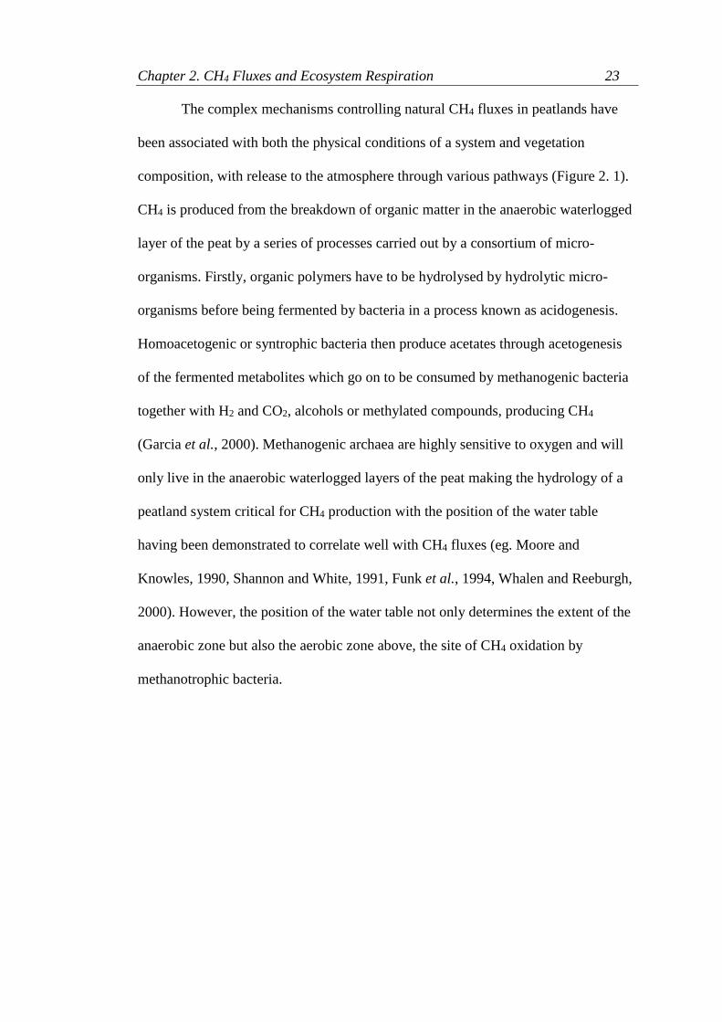
Chapter 2. CH4 Fluxes and Ecosystem Respiration 23
The complex mechanisms controlling natural CH4 fluxes in peatlands have
been associated with both the physical conditions of a system and vegetation
composition, with release to the atmosphere through various pathways (Figure 2. 1).
CH4 is produced from the breakdown of organic matter in the anaerobic waterlogged
layer of the peat by a series of processes carried out by a consortium of micro-
organisms. Firstly, organic polymers have to be hydrolysed by hydrolytic micro-
organisms before being fermented by bacteria in a process known as acidogenesis.
Homoacetogenic or syntrophic bacteria then produce acetates through acetogenesis
of the fermented metabolites which go on to be consumed by methanogenic bacteria
together with H2 and CO2, alcohols or methylated compounds, producing CH4
(Garcia et al., 2000). Methanogenic archaea are highly sensitive to oxygen and will
only live in the anaerobic waterlogged layers of the peat making the hydrology of a
peatland system critical for CH4 production with the position of the water table
having been demonstrated to correlate well with CH4 fluxes (eg. Moore and
Knowles, 1990, Shannon and White, 1991, Funk et al., 1994, Whalen and Reeburgh,
2000). However, the position of the water table not only determines the extent of the
anaerobic zone but also the aerobic zone above, the site of CH4 oxidation by
methanotrophic bacteria.

Figure 2. 1 The mechanisms for surface exchange of CO2 and CH4 in a peatland system.
Chapter 2
. CH
4 Flu
xes and E
cosystem
Resp
iratio
n 2
4

Chapter 2. CH4 Fluxes and Ecosystem Respiration 25
Various controls on methanotrophic and methanogenic activity such as soil
temperature, pH, osmotic pressure and substrate composition (Dunfield et al., 1993,
Garcia et al., 2000, Bergman et al., 1998) have been demonstrated and fire has the
potential to change these conditions thus influencing CH4 production and oxidation.
For example, above ground biomass removal due to burning may increase soil
temperatures, which can increase methogenesis (Rydin and Jeglum, 2006), by
exposing the soil surface to solar radiation (Jury and Horton, 2004). Any loss of the
Sphagnum layer could also potentially reduce the amount of CH4 oxidised by the
methanotrophs which reside there. The understanding of the effect of fire on the
Sphagnum layer is limited but some studies have shown that the Sphagnum layer
may experience biologically lethal temperatures (Davies, 2005, Glime, 2007) and can
be consumed by a fire (Hamilton 2000). There is also limited research into the effect
of fire on the bacterial community of peat soils, particularly the impact on
methanogenic bacteria (Andersen et al., 2013) but a general reduction in
methanotroph population size together with an increase in the dominance of type II
methanotrophs has been demonstrated on a burned Calluna vulgaris (L.) Hull (from
herein referred to as Calluna) dominated peatland (Chen et al., 2008). CH4 can
however also naturally bypass oxidation by methanotrophs in both the acrotelm and
the Sphagnum layer, by travelling through much more direct pathways between the
site of production and the atmosphere.
The most direct pathway for CH4 loss to the atmosphere is through steady or
episodic ebullition, where CH4 rises through the acrotelm getting released as bubbles
at the surface (Figure 2. 1). For CH4 bubbles to be produced the partial pressure of all
Chapter 2. CH4 Fluxes and Ecosystem Respiration 26
the gases in solution has to exceed the hydrostatic pressure of the peat (Chanton et
al., 1995) and grow in size (Kellner et al., 2005) to create areas of over pressurised
peat which release the bubbles to the surface by ejection or soil pore enlargement
(Kellner et al., 2004). Ebullition can be a significant pathway for the loss of CH4
over short time scales from a system (Glaser et al., 2004) and in some instances may
be the most dominant pathway for CH4 loss from a peatland (Coulthard et al., 2009).
The direct loss of CH4 to the surface may also be facilitated by the movement of CH4
through gas conduits in vegetation.
Some plants which have their roots in waterlogged anoxic soils have
developed larger aerenchyma, internal chambers allowing the movement of gasses
between the root and shoot (Jackson and Armstrong, 1999). Although facilitating the
flow of oxygen to roots and rhizomes, the outward diffusion of oxygen from
aerenchyma to the rhizosphere induces the intake of CH4, thus acting as a conduit for
CH4 to travel through the plant to the atmosphere along a diffusion gradient (Jackson
and Armstrong, 1999). A number of studies have shown how common blanket bog
species which possess aerenchyma such as Eriophorum spp. can dramatically
increase CH4 emissions from the soil (eg. Schimel, 1995, Green and Baird, 2011).
Fire can induce a change in the dominant vegetation from Calluna to Eriophorum
spp. (Jackson and Armstrong, 1999, Stewart et al., 2004, Ward et al., 2007) which
could increase direct movement of CH4 to the surface. Wetland plants can also
facilitate CH4 transport when an internal/external pressure gradient exists resulting in
the drawing up of CH4 through the plant with release to the atmosphere through
stomata or cuticle (Morrissey et al., 1992, Jackson and Armstrong, 1999). This

Chapter 2. CH4 Fluxes and Ecosystem Respiration 27
pressurised ventilation is commonly caused by thermo-osmosis, when gas flows from
young tissue, which internally has a smaller pore diameter, to old tissue and rhizomes
as a result of differences in internal and external temperatures (Grosse et al., 1991,
Whalen, 2005) and a humidity induced diffusion (Jackson and Armstrong, 1999).
The role of vascular plants in the efflux of CH4 from peatlands is also complicated by
their ability to change the soil substrate and oxygen levels in the rhizosphere and
influencing bacterial activity and CH4 production and oxidation in the soil. Radial
oxygen loss (ROL) increases oxygen levels in soil and thus may inhibit
methanogenisis (Jackson and Armstrong, 1999). This can also favour methanotrophy
which can only occur in the presence of oxygen (Chanton, 2005). However, vascular
plants may also increase bacterial activity, including methanogenesis, in peatlands by
increasing the availability of organic carbon through root exudation (Öquist and
Svensson, 2002). This complex relationship between vascular plants and CH4
production, oxidation and CH4 release means understanding how fire may bring
about changes in vegetation is not only important for the surface exchange of CO2.
2.3 Aims
The aim of this study was to measure short term (<3 years) CH4 fluxes and
Ecosystem Respiration (ER) from areas of burnt blanket bog while concurrently
measuring fluxes on adjacent unburnt control plots. Specifically, the study aimed to
establish sampling sites in areas where fires had characteristics akin to those of
management fires which follow the best practice guidance, namely being quick
moving consuming mostly just the upper vegetation canopy and leaving the moss
layer intact. In addition, vegetation composition, soil temperature, soil moisture and

Chapter 2. CH4 Fluxes and Ecosystem Respiration 28
position of the water table were measured to see how well these measurements could
explain observed fluxes and if any differences in these potential controls on carbon
cycling could be found between burnt and unburnt blanket bog. It was intended that
CH4 fluxes be measured as soon as possible after a fire to determine if there was a
short term increase in CH4 emissions as has been found previously (Gray 2006). It
was hypothesised that [1] CH4 emissions would be significantly higher at burnt plots
when compared to unburnt plots immediately after the fire, as seen by Gray (2006),
when changes in the vegetation and abiotic conditions could be most different
between treatments and [2] ER would be significantly different between burnt and
unburnt plots due to the change in vegetation composition and abiotic factors brought
about by fire. These assumptions led to hypothesis [3] that CH4 and Ecosystem
Respiration would be related to vegetation, water table position soil temperature and
soil moisture conditions.
2.4 Methodology
2.4.1 Site descriptions
Three study sites were established across Scotland, in Caithness, the Eastern
Grampians and in the Pentlands (Table 2. 1). First to be established in April 2011
was a wildfire site situated within the Flow Country, Caithness, Northern Scotland,
2km south of Forsinard (Appendix 2.1). Study plots were located within an area of
Sphagnum papillosum/Eriophorum vaginatum dominated blanket bog, most closely
attributed to the JNCC UK National Vegetation Classification (NVC) M17a Scirpus
cespitosus – Eriophorum vaginatum blanket mire Drosera – Sphagnum sub
community (further details on NVC classifications are given in Chapter 5). The site

Chapter 2. CH4 Fluxes and Ecosystem Respiration 29
had been burnt by a wildfire most likely originating from a passing steam train on the
nearby railway tracks. Although no information was available on the specific
characteristics of the fire it was quick moving and consumed canopy vegetation and
small discrete patches of the Sphagnum lawn and hummocks, but in the area sampled
did not penetrate the peat. The climate at Forsinard can be described as cool and wet
with mean annual temperatures of between 7.5-8.0°C with an annual precipitation
ranging between 650-1000mm (Centre for Ecology and Hydrology, 2012). 12 plots
were established at the site, on the southern edge of the fire, with 6 situated either
side of the fire edge on burnt and unburnt ground.
Second to be established in March 2012 was a site situated on Eastside Farm
in the Pentlands (Appendix 2.1). Dominated by Calluna and Eriophorum vaginatum
the area is burned under a rotated muirburn regime primarily to maintain palatable
grazing for sheep. The area sampled lies over peat between 40 and 125cm in depth
with some wetter areas dominated by Sphagnum capillifolium (Ehrh.) Hedw. and
Sphagnum fallax (Klinggr.) Klinggr. Historically drains have been cut in an effort to
dry the area, however, over time some have become blocked resulting in a patchwork
of wetter/dryer areas dominated by Eriophorum spp. and Calluna respectively. In the
areas which were studied (Calluna dominated) the vegetation could best be described
as NVC community M20b Eriophorum vaginatum mire: Calluna vulgaris- Cladonia
sub community. A total of 14 randomly located plots were established at this site, 7
burnt and 7 unburnt plots. Unburnt plots were established on areas which did not
naturally burn while others were located on areas where fire retardant hoods, made
from fire retardant woven glass fibre material (FirePro PU28), had been placed to
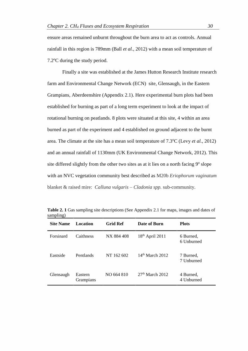
Chapter 2. CH4 Fluxes and Ecosystem Respiration 30
ensure areas remained unburnt throughout the burn area to act as controls. Annual
rainfall in this region is 789mm (Ball et al., 2012) with a mean soil temperature of
7.2oC during the study period.
Finally a site was established at the James Hutton Research Institute research
farm and Environmental Change Network (ECN) site, Glensaugh, in the Eastern
Grampians, Aberdeenshire (Appendix 2.1). Here experimental burn plots had been
established for burning as part of a long term experiment to look at the impact of
rotational burning on peatlands. 8 plots were situated at this site, 4 within an area
burned as part of the experiment and 4 established on ground adjacent to the burnt
area. The climate at the site has a mean soil temperature of 7.3oC (Levy et al., 2012)
and an annual rainfall of 1130mm (UK Environmental Change Network, 2012). This
site differed slightly from the other two sites as at it lies on a north facing 9o slope
with an NVC vegetation community best described as M20b Eriophorum vaginatum
blanket & raised mire: Calluna vulgaris – Cladonia spp. sub-community.
Table 2. 1 Gas sampling site descriptions (See Appendix 2.1 for maps, images and dates of
sampling)
Site Name Location Grid Ref Date of Burn Plots
Forsinard
Caithness
NX 884 408 18th April 2011
6 Burned,
6 Unburned
Eastside
Pentlands
NT 162 602
14th March 2012 7 Burned,
7 Unburned
Glensaugh Eastern
Grampians NO 664 810 27th March 2012 4 Burned,
4 Unburned
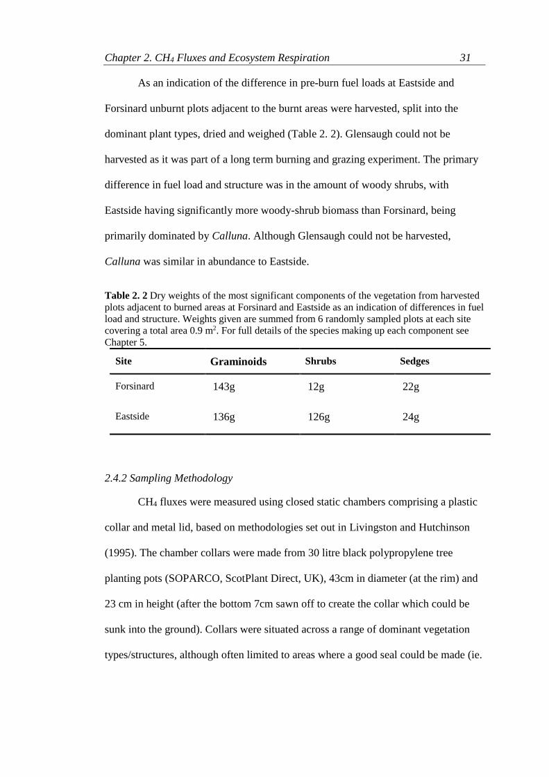
Chapter 2. CH4 Fluxes and Ecosystem Respiration 31
As an indication of the difference in pre-burn fuel loads at Eastside and
Forsinard unburnt plots adjacent to the burnt areas were harvested, split into the
dominant plant types, dried and weighed (Table 2. 2). Glensaugh could not be
harvested as it was part of a long term burning and grazing experiment. The primary
difference in fuel load and structure was in the amount of woody shrubs, with
Eastside having significantly more woody-shrub biomass than Forsinard, being
primarily dominated by Calluna. Although Glensaugh could not be harvested,
Calluna was similar in abundance to Eastside.
Table 2. 2 Dry weights of the most significant components of the vegetation from harvested
plots adjacent to burned areas at Forsinard and Eastside as an indication of differences in fuel
load and structure. Weights given are summed from 6 randomly sampled plots at each site
covering a total area 0.9 m2. For full details of the species making up each component see
Chapter 5.
Site Graminoids Shrubs Sedges
Forsinard 143g 12g 22g
Eastside 136g 126g 24g
2.4.2 Sampling Methodology
CH4 fluxes were measured using closed static chambers comprising a plastic
collar and metal lid, based on methodologies set out in Livingston and Hutchinson
(1995). The chamber collars were made from 30 litre black polypropylene tree
planting pots (SOPARCO, ScotPlant Direct, UK), 43cm in diameter (at the rim) and
23 cm in height (after the bottom 7cm sawn off to create the collar which could be
sunk into the ground). Collars were situated across a range of dominant vegetation
types/structures, although often limited to areas where a good seal could be made (ie.

Chapter 2. CH4 Fluxes and Ecosystem Respiration 32
where they could be sunk far enough into the peat, on average 11cm). A flat metal lid
was clamped onto the collars using 10 x 15 cm spring ratchet clamps which
compressed a ring of rubber draft excluder between collar rim and lid. Each lid had a
3 way valve (Discofix ® C 3-way Stopcock) secured and sealed within the lid and a
5cm length of flexible tubing (Bev-a-Line®) attached to the valve reaching within the
chamber. Once the lid was sealed 100ml headspace samples were immediately
removed (time zero) and on three more occasions thereafter at 15 to 30 minute
intervals (with the time of sampling recorded accurate to within 3 seconds). The
syringe was slowly pumped twice with the headspace air prior to each sample
removal to aid headspace mixing within the chamber. Each sample was removed
slowly to reduce the effect of the pressure change within the chamber, which could
induce methane diffusion to the surface. 25ml glass vials were pre-sealed with an
aluminium cap and pre-fitted silicone septa (National Scientific Company,
Rockwood) and filled with the sample headspace air by using an additional needle
inserted into the cap so the entire 100ml sample could be flushed through the vial,
eliminating the need to pre-evacuate the vials. Both the additional needle and sample
needle were removed from the cap before flushing was complete to ensure external
air was not pulled into the vial. Immediately after sampling volumetric soil water
content, referred to as soil moisture (SM), was measured using a HydrosenseTM 20cm
probe (HydrosenseTM CS620, Campbell Scientific) and soil temperature (ST)
recorded using a digital temperature sensor with 12cm probe (Digitron 2080R, Sifam
Instruments Ltd.), both measurements being taken in the soil inside each chamber.
Dipwells made from 4cm diameter plumbing pipe between 80cm and 120cm in

Chapter 2. CH4 Fluxes and Ecosystem Respiration 33
length, with 6mm holes drilled on three sides every 12cm down their length, were
sunk vertically into the peat adjacent to each chamber. The distance to the water table
(WT) was measured as the distance from the surface of the peat/moss interface to the
surface of the water in each dipwell. Headspace volume of each chamber was
estimated by measuring the depth of each chamber (distance from the rim of the
chamber to the ground) at 5 locations in the chamber. The ground was defined as the
point a ruler could not easily be pushed down any lower so included areas of dense
vegetation with little airspace, as well as the point at which the ruler hit the peat
surface. Volume (m3) was calculated using equation 2.1, where A is the area of
chamber and mD is the mean depth of the chamber.
𝑣 = 𝐴 × 𝑚𝐷
Eq 2. 1
2.4.3 Gas Chromatography
Samples were analysed within 7 days from time of sampling using a Gas
Chromatograph fitted with a flame ionisation detector (HP5890 Series II, Hewlett
Packard, Agilent Technologies UK Ltd, Stockport, UK) and 50 sample autosampler
(Genesis Headspace Sampler, Varian®). To calculate concentrations of the field
samples four standard gases were used with known concentrations of CO2 and CH4.
These standard samples were analysed at the start and end of each run of field
samples and every 12 field samples throughout an analysis run to minimise the effect
of any drift in the voltage signal of the gas chromatograph. The area under each
output peak (in mV) of each sample was calculated using Clarity Chromatography

Chapter 2. CH4 Fluxes and Ecosystem Respiration 34
Software (v.3.0.6.589). A linear regression was used to calibrate the peak area with
the known concentrations of the four standard samples. This allowed the calculation
of the concentrations of CO2 and CH4 in the unknown field samples.
2.4.4 Flux Calculations
Using the calculated concentrations of each field sample and the recorded
time of sampling, a flux could be calculated for each chamber using the software
GCFlux V2 (Levy, 2012). To calculate a flux in µmol m2 s-1 equation 2.2 was used
where: dC is the initial rate of change in concentration (µmol mol-1), dt is the rate of
change in time (s), p is the density of air (mol m3), V is volume of the chamber
headspace (m3) and A is the surface area of the soil or vegetation (m2) (Levy et al.,
2011).
𝐹𝑙𝑢𝑥 (𝑢𝑚𝑜𝑙 𝑚2 𝑠−1) = 𝑑𝐶
𝑑𝑡×
𝑝𝑉
𝐴
Eq 2. 2
To establish if CH4 fluxes were linear, CO2 sample concentrations, valid in
respect to errors in sampling or from the sealing efficiency of the chambers, were
used as a comparison. Where CO2 fluxes were positive and looked linear, with no
drop in concentration over time, it was assumed that the chambers had sealed well
and therefore the CH4 concentrations calculated were valid. Where an unexpectedly
low concentration of CO2 was found for a sample, departing from a general increase
in CO2 over time, the sample was rejected and not used when calculating CH4 fluxes
as it was assumed there was an error when sampling. Likewise, if no steady increase
in CO2 was observed, with concentrations staying around ambient, it was assumed
Chapter 2. CH4 Fluxes and Ecosystem Respiration 35
the chamber was not sufficiently sealed and the CH4 flux calculated for the chamber
was not valid and omitted from further analysis.
2.4.5 Vegetation Assessment
Flux measurements were repeated on the same plots at each site for a period
of up to two and a half years, with harvesting of plant biomass on the final day of
sampling (766 days since the site was burned at Forsinard and 439 days at Eastside).
Plots at Glensuagh could not be harvested as they were within the boundary of a
long-term grazing experiment so vegetation could not be disturbed on site.
Vegetation at each plot was separated from the peat surface and removed. Within 2
days the vegetation was sorted into species with Calluna and graminoids further
sorted into “green” and “woody/brown” components. To measure dry weight each
sub-sample was dried in an oven at 70oC for a maximum of 12 days or until samples
no longer lost weight and weighed. Prior to drying, the leaf area of 3 leaves/blades of
each species (3 samples of green leaves and finer branches in the case of Calluna)
were measured using an area meter (Licor LI3100C, Licor) and weighed once dried
to allow for a calculation of leaf area (cm3) per gram dry weight (gdw). Total leaf area
of each species could then be extrapolated from total dry weight per species.
Percentage cover of Sphagnum spp. per plot was used in the analysis instead of leaf
area which could not be accurately calculated.
To evaluate the relationship between vegetation composition and CH4 fluxes
and ER only fluxes measured on the final day of sampling were used. It was not
deemed appropriate to compare the vegetation data to fluxes calculated across the
Chapter 2. CH4 Fluxes and Ecosystem Respiration 36
whole sampling period due to changes in vegetation over time, particularly in the
burnt plots.
2.4.6 Statistical Analysis
Paired two-sample t tests were used to compare SM, ST and WT between
burned and unburned plots measured on the same day. When the data was not
normally distributed, or when sample sizes were small (such as at the Glensaugh
site), a Wilcoxon signed rank test was used. One-Way Analysis of Variance
(ANOVA) was used to show any significant differences in ST, SM and WT between
sites and CH4 and ER between sites.
In order to evaluate any treatment effect, as well any relationship with
measured abiotic factors, on CH4 and ER, linear mixed effects models were used to
allow for the dependence of the calculated fluxes, as they were repeated
measurements made at the same plots over time. By allowing for random effects the
models could also be used to evaluate within and between site variation in fluxes.
CH4 fluxes and ER were log transformed to meet model assumptions and modelled
separately with the same fixed and random effects terms (Table 2. 3). Random effect
terms were assessed first using Akaike Information Criterion (AIC) computed from
Restricted Maximum Likelihood (REML) parameter estimates with the amount of
variance explained by each term in the model assessed and terms discarded until a
model was established which had the smallest AIC and composed of the most
relevant random effect terms. As there was only one fixed effect (treatment) this was
kept in all models to show its significance with a Wald test. All statistics were
Chapter 2. CH4 Fluxes and Ecosystem Respiration 37
carried out using the statistical program R (v R i386 3.0.1) (R Core Team, 2013) with
mixed effects modelling computed using the package lme4 (Bates et al., 2013).
Table 2. 3 Fixed and random effects terms used in mixed effects modelling of CH4 fluxes
and ecosystem respiration (ER).
2.5 Results
2.5.1 Soil Moisture, Water table and Soil Temperature
Measurements were made across a range of conditions; soil temperature
varying from 3oC to 10oC, soil moisture from 20 to 100% and water table position
36cm below the surface to being at the surface (Appendix 2.2). In general
measurements were made in drier conditions at Glensaugh (F(2,339)=14.74,
Model Term Abbreviation Description
Fixed Effects
Treatment
Burnt or unburnt
Random Effects (accounting for variance within Treatment)
Plot P Plot
Day D
The day plots were sampled given as the
number of days since the site had been
burnt
Site S Site
Water table WT Distance from height of water within
dipwell to peat surface (cm)
Soil Moisture SM Volumetric soil water content (%)
Soil Temperature ST Temperature of the soil at each plot (oC)
Site:Plot S:P Plot nested within Site to specify variance
between plots at the same site
Site:Day S:D Day nested within Site to specify variance
between days at the same site

Chapter 2. CH4 Fluxes and Ecosystem Respiration 38
p=<0.001) while a wider range of soil temperatures were recorded at Eastside. Soil
temperature, soil moisture and position of the water table varied between plots, with
a strong seasonal pattern found for soil temperature with warmer temperatures seen
during summer months. Greatest variation in water table position was found between
plots at Eastside, with the most homogeneous conditions found in the plots at
Forsinard. No significant differences in soil temperature, soil moisture or water table
position were found between burnt and unburnt plots at any site.
2.5.2 CH4 Fluxes
CH4 fluxes ranged from 0.03 to 557.60 nmol m2 s-1 and were significantly
different between sites (F(2,160)=6.3, p=0.01) and varied considerably between
plots and over time (Table 2. 4, Appendix 2.3). However, the linear mixed effects
modelling showed no significant treatment effect on the measured fluxes at any site
(Figure 2. 2, Table 2. 5). The random effects which best accounted for variation in
fluxes were plot, day, water table and soil temperature. Plot to plot variation within
site explained the most variance (Figure 2. 3) but the amount of residual variation
suggests there was a lot of variation not accounted for by the model (Figure 2. 3).
Despite being a component of the most appropriate model with the lowest AIC soil
temperature and water table accounted for little of the variation in fluxes.

Chapter 2. CH4 Fluxes and Ecosystem Respiration 39
Table 2. 4 CH4 fluxes at each site and treatment (nmol m2 s-1±StE)
Site Plots Min Max Mean
Eastside All
Burnt
Unburnt
0.03
0.03
0.08
557.60
557.60
164.10
30.4±11.1
45.1±23.3
17.9±15.5
Forsinard All
Burnt
Unburnt
0.99
0.99
1.25
43.65
41.12
43.65
14.6±1.3
16.3±1.9
12.8±1.8
Glensaugh
All
Burnt
Unburnt
0.24
0.24
0.49
98.59
29.32
98.59
20.8±4.8
13.9±5.6
26.7±7.5
Figure 2. 2 CH4 fluxes at each site (E=Eastside, G=Glensaugh, F=Forsinard) under each
treatment where bold lines show median value, horizontal edges of boxes upper and lower
quartiles, end of lines smallest and largest values and outliers circles. Only valid samples
used in analysis (n). Positive numbers indicate CH4 release to the atmosphere.
0
50
100
150
200
E F G
Site
CH
4 F
lux
(nm
ol C
H4
m2
s1)
Treatment
B
UB
n=34
n=29
n=36 n=34
n=14
n=16
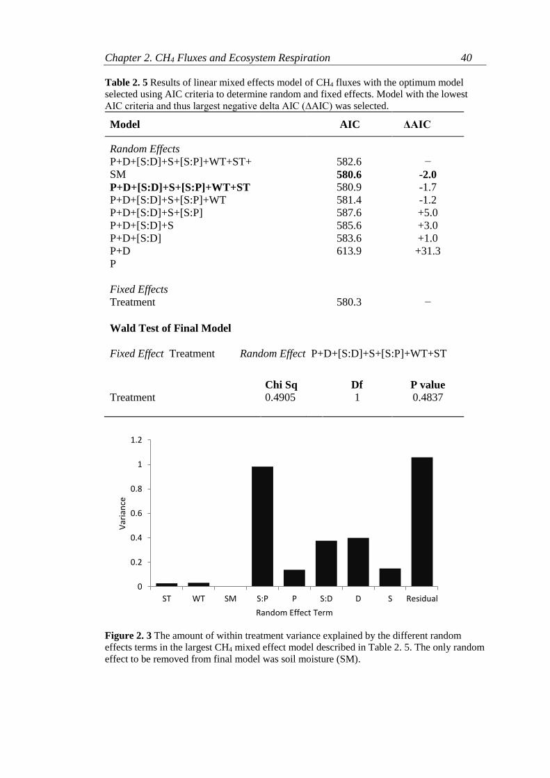
Chapter 2. CH4 Fluxes and Ecosystem Respiration 40
Table 2. 5 Results of linear mixed effects model of CH4 fluxes with the optimum model
selected using AIC criteria to determine random and fixed effects. Model with the lowest
AIC criteria and thus largest negative delta AIC (∆AIC) was selected.
Model AIC ΔAIC
Random Effects
P+D+[S:D]+S+[S:P]+WT+ST+
SM
P+D+[S:D]+S+[S:P]+WT+ST
P+D+[S:D]+S+[S:P]+WT
P+D+[S:D]+S+[S:P]
P+D+[S:D]+S
P+D+[S:D]
P+D
P
Fixed Effects
Treatment
582.6
580.6
580.9
581.4
587.6
585.6
583.6
613.9
580.3
−
-2.0
-1.7
-1.2
+5.0
+3.0
+1.0
+31.3
−
Wald Test of Final Model
Fixed Effect Treatment Random Effect P+D+[S:D]+S+[S:P]+WT+ST
Chi Sq Df P value Treatment 0.4905 1 0.4837
Figure 2. 3 The amount of within treatment variance explained by the different random
effects terms in the largest CH4 mixed effect model described in Table 2. 5. The only random
effect to be removed from final model was soil moisture (SM).
0
0.2
0.4
0.6
0.8
1
1.2
ST WT SM S:P P S:D D S Residual
Var
ian
ce
Random Effect Term
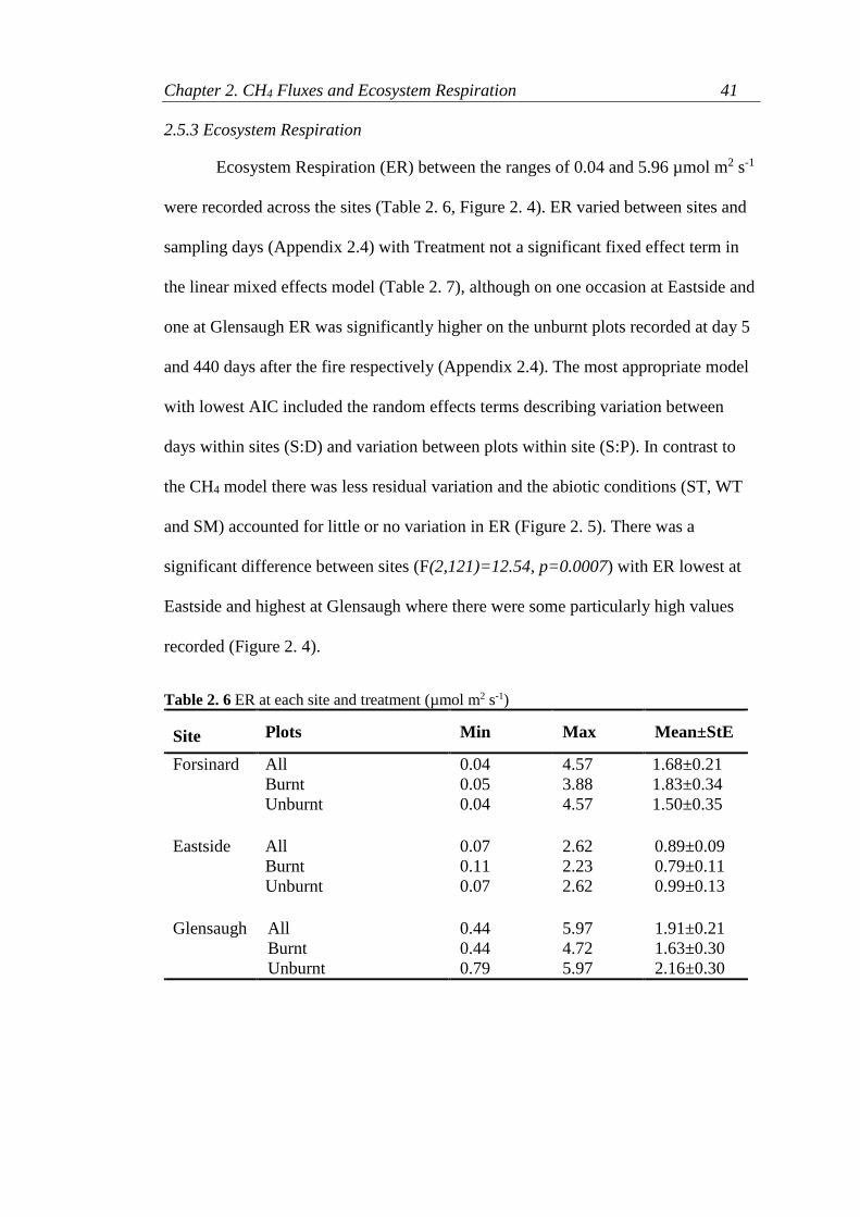
Chapter 2. CH4 Fluxes and Ecosystem Respiration 41
2.5.3 Ecosystem Respiration
Ecosystem Respiration (ER) between the ranges of 0.04 and 5.96 µmol m2 s-1
were recorded across the sites (Table 2. 6, Figure 2. 4). ER varied between sites and
sampling days (Appendix 2.4) with Treatment not a significant fixed effect term in
the linear mixed effects model (Table 2. 7), although on one occasion at Eastside and
one at Glensaugh ER was significantly higher on the unburnt plots recorded at day 5
and 440 days after the fire respectively (Appendix 2.4). The most appropriate model
with lowest AIC included the random effects terms describing variation between
days within sites (S:D) and variation between plots within site (S:P). In contrast to
the CH4 model there was less residual variation and the abiotic conditions (ST, WT
and SM) accounted for little or no variation in ER (Figure 2. 5). There was a
significant difference between sites (F(2,121)=12.54, p=0.0007) with ER lowest at
Eastside and highest at Glensaugh where there were some particularly high values
recorded (Figure 2. 4).
Table 2. 6 ER at each site and treatment (µmol m2 s-1)
Site Plots Min Max Mean±StE
Forsinard All
Burnt
Unburnt
0.04
0.05
0.04
4.57
3.88
4.57
1.68±0.21
1.83±0.34
1.50±0.35
Eastside All
Burnt
Unburnt
0.07
0.11
0.07
2.62
2.23
2.62
0.89±0.09
0.79±0.11
0.99±0.13
Glensaugh
All
Burnt
Unburnt
0.44
0.44
0.79
5.97
4.72
5.97
1.91±0.21
1.63±0.30
2.16±0.30

Chapter 2. CH4 Fluxes and Ecosystem Respiration 42
Figure 2. 4 Ecosystem Respiration (ER) at each site (E=Eastside, G=Glensaugh,
F=Forsinard) under each treatment where bold lines show median value, horizontal edges of
boxes upper and lower quartiles, end of lines smallest and largest values and outliers circles.
Only valid samples used in analysis (n). Positive numbers indicate CO2 release to the
atmosphere.
0
2000
4000
6000
E F G
Site
ER
(n
mol C
O2
m2
s1)
Treatment
B
UB
n=30
n=31
n=18
n=15 n=14
n=16

Chapter 2. CH4 Fluxes and Ecosystem Respiration 43
Table 2. 7 Results of linear mixed effects model of ER with the optimum model selected
using AIC criteria to determine random and fixed effects. Models with the lowest AIC
criteria and thus largest negative delta AIC (∆AIC) were selected.
Model AIC
ΔAIC
Random Effects
D+[S:D]+[S:P]+S+ST+P+SM+
WT
D+[S:D]+[S:P]+S+ST+P+SM
D+[S:D]+[S:P]+S+ST+P
D+[S:D]+[S:P]+S+ST
D+[S:D]+[S:P]+S
D+[S:D]+[S:P]
D+[S:D]
D
Fixed Effects
Treatment
289.2
287.2
285.2
283.5
283.9
282.0
296.3
294.3
279.7
−
-2.0
-4.0
-5.7
-5.3
-7.2
+7.1
+5.1
−
Wald Test of Final Model
Fixed Effect Treatment Random Effect D+[S:D]+[S:P]
Chi Sq Df P value Treatment 0.654 1 0.4187
Figure 2. 5 The amount of within treatment variance explained by the different random
effects terms in the largest ER mixed effect model described in Table 2. 7.
The only random effect terms kept in the final model were D, S:D and S:P.
0
0.1
0.2
0.3
0.4
0.5
0.6
0.7
Var
ian
ce
Random Effect Term

Chapter 2. CH4 Fluxes and Ecosystem Respiration 44
2.5.4 Fluxes and Vegetation
No clear relationship was found between any measure of vegetation (biomass,
leaf area or species composition) and CH4 fluxes or ER at Forsinard or Eastside
(Glensaugh was not harvested) (Figure 2. 6, Figure 2. 7) even when included as
random effects in the linear mixed effects models of CH4 emissions and ER (not
reported). A more detailed discussion of vegetation composition at the sites is given
in Chapter 5 but in general Sphagnum spp. cover was greatest at Forsinard with only
3 plots at Eastside containing Sphagnum spp and similar ranges of total vascular
plant biomass, leaf area and Eriophorum spp. dry weight were found at the two sites.
The vegetation at the two sites did match to different National Vegetation
Classification sub communities, with the greatest uniformity in vegetation found
between the plots at Forsinard.

Chapter 2. CH4 Fluxes and Ecosystem Respiration 45
Figure 2. 6 Methane fluxes at each plot plotted against (a) total vascular plant biomass, (b)
total vascular plant leaf area, (c) total percent Sphagnum spp. cover and (d) total Eriophorum
spp. dry weight with r2 values and p values (shown in brackets). Triangles represent
Forsinard plots (n=10), circles Eastside (n=6), black points burnt plots and grey unburnt.
r2= 0.05 (0.54)
r2= 0.14 (0.46)
r2= 0.01 (0.79)
r2= 0.09 (0.56)
r2= 0.001 (0.93)
r2= 0.04 (0.71)
r2= 0.02 (0.68)
r2= 0.23 (0.33)
(c)
(a) (b)
(d)

Chapter 2. CH4 Fluxes and Ecosystem Respiration 46
Figure 2. 7 Ecosystem Respiration (ER) at each plot plotted against (a) total vascular plant
biomass, (b) total vascular plant leaf area, (c) total percent Sphagnum spp. cover and (d) total
Eriophorum spp. dry weight with r2 values and p values (shown in brackets). Triangles
represent Forsinard plots (n=10), circles Eastside (n=6), black points burnt plots and grey
unburnt.
r2= 0.02 (0.79)
r2= 0.21 (0.36)
r2= 0.01 (0.73)
r2= 0.12 (0.50)
r2= 0.14 (0.28)
r2= 0.05 (0.65)
r2= 0.03 (0.79)
r2= 0.25 (0.31)
(c)
(a) (b)
(d)

Chapter 2. CH4 Fluxes and Ecosystem Respiration 47
2.6 Discussion
2.6.1 CH4 fluxes
There was no significant difference in CH4 fluxes between burnt and unburnt
control plots at any of the three sites studied. Fluxes recorded are consistent with
those previously reported on blanket bog in the UK (eg. Hargreaves and Fowler,
1998, Ward et al., 2007, Dinsmore et al., 2009, Loyd, 2010, Levy et al., 2012,
Stockdale, 2012) and were of a similar range as those recorded by Gray (2006) at an
area of blanket bog which had been burned close to the area studied here at
Forsinard. Therefore hypothesis [1], CH4 emissions would be significantly higher in
burnt plots when compared to unburnt plots, has to be rejected. Previous studies
which have measured CH4 fluxes on burnt and unburnt blanket bog have been
contradictory and shown that burning was both associated with an increase in CH4
emissions immediately after burning as with Gray (2006), and a reduction in CH4
emissions on burnt plots when compared to unburnt plots (Ward et al., 2007). Taken
with the results of this study the effect of burning on CH4 fluxes therefore still seems
to be inconsistent.
Determining the effect of fire on blanket bog is confounded by fire not being
a standard treatment, instead one which varies in its severity (Hobbs and
Gimingham, 1984) and frequency (Yallop et al., 2006), both factors which may
influence the impact of fire on an ecosystem (Schimmel and Granstrom, 1996, Neary
et al., 1999). Ecosystem response to fire may also be related to ecosystem state and
vegetation structure and composition pre-burn (Davies et al., 2010). This makes it
necessary to put the fires studied here into context as they did not affect the peat and

Chapter 2. CH4 Fluxes and Ecosystem Respiration 48
consumed little of the moss layer, removing just the top canopy shrubs and
graminoids. Therefore, the results imply that fires which have no impact on the
substrate do not affect CH4 fluxes of blanket bogs in the medium term (less than
three years as measured here). It has been widely shown that fires which do penetrate
the peat cause significant carbon loss to the atmosphere (Turetsky and Wieder, 2001,
Davies et al., 2013) and it is important to reiterate the distinction between these types
of fire and the fires studied here.
In addition to the characteristics of a fire, it may also be important when
considering the long term impacts of a fire on vegetation and carbon cycling to
consider fire history. The sites studied here are all likely to have seen some managed
burning and wildfires in the past, but not at the frequency of the site studied by Ward
et al. (2007). Frequent burning and its potential to induce changes in vegetation
composition (Gray, 2006, Worrall et al., 2007, Ward et al., 2012) promoting
aerenchymatous species such as Eriophorum angustifolim (Jackson and Armstrong,
1999, Stewart et al., 2004, Ward et al., 2007), may be important in explaining
associated increases in methane emissions from blanket bog post burn in the long
term, by increasing plant mediated transport to the atmosphere. Although this study
did not show any relationship between CH4 fluxes and cover or biomass of
vegetation, fluxes were measured in the dark so the lack of correlation between the
aerenchymatous Eriophorum spp. and CH4 fluxes as has been demonstrated
previously (McNamara et al., 2008) could be a result of reduced active transport of
CH4 brought about by the closure of stomata (Frye et al., 1994, Thomas et al., 1996),
although others have reported no differences in steady CH4 flux in light and dark

Chapter 2. CH4 Fluxes and Ecosystem Respiration 49
phases (Green and Baird, 2011). Overall the results here suggest that vegetation was
not a good indicator of CH4 emissions at the sites studied, a rejection of hypothesis
[3], with the considerable variation in fluxes both between sites and sampling days
more associated with abiotic conditions which did vary considerably both spatially
and temporally.
Measured CH4 fluxes have been shown to relate to the interplay between
conditions such as the position of the water table and the vegetation within a
chamber (Dinsmore et al., 2009), so the large variability in conditions between sites,
plots and sampling date may perhaps mask any more subtle associations between
CH4 and vegetation. The CH4 fluxes recorded here varied considerably over time,
between plots and sites with plot to plot variation within site explaining the greatest
amount of variance in the mixed effects model. This high variability in CH4
emissions has been commonly reported by studies which have measured CH4 over
longer periods (Lai, 2009)
Despite the position of the water table and soil temperature not being
measured continuously, being more “snap-shot” measurements with some seasonal
bias due to the dates of sampling, both were significant random effect terms in the
model. This is consistent with the literature where water table and soil temperature
have been found to correlate with CH4 emissions (Moore and Knowles, 1990,
Shannon and White, 1991, Funk et al., 1994, Hargreaves and Fowler, 1998, Whalen
and Reeburgh, 2000, Rydin and Jeglum, 2006). This, to a large extent, can help
explain the significance of sampling date, plot and site in the models as conditions
varied at all these scales. The model does however also suggest that using water table
Chapter 2. CH4 Fluxes and Ecosystem Respiration 50
or soil temperature alone as indicators of CH4 emissions, particularly when upscaling
to estimate, for example annual or catchment carbon budgets, may underestimate the
variability in emissions as there was a large amount of residual variation not
explained by the model here.
2.6.2 Ecosystem Respiration
ER was found to be significantly lower on burnt plots compared to unburnt
plots on two occasions from a total of 13 sampling days, but after considerably
different periods of time from when the sites were burnt suggesting no trend in
treatment effect. However, when taking the results of the model into account
hypothesis [2] has to be rejected as ER of burnt plots was not significantly different
to those of unburnt control plots in the vast majority of sampling times, with
treatment not significant when considered a fixed effect and sampling date, site, plot
and measured abiotic variables random effects in the model. This contradicts
previous findings by Ward et al. (2007) who found that ER was higher at a site
burned every 10 years compared to a no burn control site at the Hard Hill experiment
at Moor House. Clay et al., (2010) at the same site also found that burning had a
significant effect on ER but only in conjunction with grazing. The results here show
that fire did not have an effect on ER and contradicts the finding of Clay et al.,
(2010) as both Glensaugh and Eastside were also grazed. The fires studied here were
of course quick moving low severity fires which may make them different to those
experienced at Hard Hill and again reiterates the importance of taking the
characteristics of a fire into account when discussing the impact of a fire on carbon
cycling.
Chapter 2. CH4 Fluxes and Ecosystem Respiration 51
As with the CH4 fluxes recorded, ER varied between sites and sampling days
and falls within the ranges previously reported for blanket bogs (eg. Bubier et al.,
1998, Bubier et al., 2003, Lafleur et al., 2005, Gazovic et al., 2013, Strack et al.,
2014) including those recorded by Ward et al. (2007) at Hard Hill. The significance
of sampling day found here is consistent with previous studies which have also found
ER to vary significantly between sampling days as well as season and year (Ward et
al., 2007, McNamara et al., 2008). Thermal regime and hydrology are considered
important controls on soil respiration (eg. Bridgham and Richardson, 1992, Silvola et
al., 1996, Scanlon and Moore, 2000, Reichstein et al., 2003) and will both vary over
different temporal and geographic scales as was the case at the three sites studied
here. Although the results here did not show any significant relationship between ER
and soil temperature, water table or soil moisture this is not inconsistent with
previous field studies on peatlands which have found no, or only weak, correlations
between ER and thermal and hydrological regimes (Updegraff et al., 2001, Lafleur et
al., 2005, Dimitrov et al., 2010) with complex relations between the two (Bubier et
al., 2003, Lafleur et al., 2003). There are also further interactions between ER and
vegetation composition and micro-habitat (Bubier et al., 2003). Previous research has
shown for example that some species such as Eriophorum spp. (McNamara et al.,
2008) and Juncus spp. (Stockdale, 2012) are associated with higher ER than
Sphagnum spp. and grasses. Here, however, no strong correlations between ER and
Eriophorum spp. biomass, leaf area or any of the measures of vegetation were found
so Hypothesis [3], ER would be related to vegetation, water table position soil
temperature and soil moisture conditions, must also be rejected in this instance.
Chapter 2. CH4 Fluxes and Ecosystem Respiration 52
2.7 Conclusions
The hypotheses that CH4 emissions and ER would be significantly higher in
burnt plots, when compared to unburnt plots, immediately after a fire have to be
rejected as there was no significant treatment effect detected when spatial and
temporal variation were taken into account. Although a weak correlation was found
between CH4 emissions and position of the water table and soil temperature they did
not vary significantly between treatments which means the results suggest that fires
that do not change these conditions, for example by penetrating the peat increasing
oxidation and drying, do not affect CH4 emissions. There were no correlations found
between CH4 emissions and measures of vegetation, including the abundance of
aerenchymatous species commonly associated with greater CH4 emissions. This
suggests that when considered alone fire induced changes in abundance of species
such as Eriophorum spp. may not always result in an increase in CH4 emissions.
Although this study only considers two components of a blanket bogs carbon
cycle, CH4 emissions and ER, important conclusions can be drawn which have a
wider relevance. The results presented here show that there are complex controls on
both CH4 emissions to the atmosphere and ER, of which the fires here did not
significantly modify to give a significant treatment effect. This means that the impact
of fire on the carbon cycling of blanket bogs is difficult to predict, particularly if the
characteristics of a fire, such as the extent it penetrates the peat and damages the
moss layer, are not taken into consideration. The results here also contradict results
from the Hard Hill experiment suggesting that the fires, the burning rotation times
and site conditions may not be representative of fires on blanket bog burned for

Chapter 2. CH4 Fluxes and Ecosystem Respiration 53
management purposes in differing circumstances. This shows the need for studies to
be carried out over a wider geographic area, particularly pertinent when seeing the
variability in CH4 and ER between the three sites studied here.

Chapter 2. CH4 Fluxes and Ecosystem Respiration 54
2.8 References
ANDERSEN, R., CHAPMAN, S. J. & ARTZ, R. R. E. 2013. Microbial communities
in natural and disturbed peatlands: A review. Soil Biology and Biochemistry,
57, 979-994.
BALL, T., BLACK, A. R. & MACDONALD, A. M. 2012. 120 year records of
spring flows in the Pentland Hills, Midlothian: geological controls and
response to drought. British Hydrological Society Annual Symposium. .
Dundee.
BATES, D., MAECHLER, M. & BOLKER, B. 2013. lme4: Linear mixed-effects
models using S4 classes. R package version 0.999999-2. http://CRAN.R-
project.org/package=lme4.
BERGMAN, I., SVENSSON, B. H. & NILSSON, M. 1998. Regulation of methane
production in a Swedish acid mire by pH, temperature and substrate. Soil
Biology & Biochemistry, 30, 729-741.
BRIDGHAM, S. D. & RICHARDSON, C. J. 1992. Mechanisms controlling soil
respiration (CO2 and CH4) in southern peatlands. Soil Biology and
Biochemistry, 24, 1089-1099.
BUBIER, J. L., BHATIA, G., MOORE, T. R., ROULET, N. T. & LAFLEUR, P. M.
2003. Spatial and Temporal Variability in Growing-Season Net Ecosystem
Carbon Dioxide Exchange at a Large Peatland in Ontario, Canada.
Ecosystems, 6, 353-367.
BUBIER, J. L., CRILL, P. M., MOORE, T. R., SAVAGE, K. & VARNER, R. K.
1998. Seasonal patterns and controls on net ecosystem CO2 exchange in a
boreal peatland complex. Global Biogeochemical Cycles, 12, 703-714.
CENTRE FOR ECOLOGY AND HYDROLOGY. 2012. CEH Carbon Catchments:
Forsinard [Online]. Available:
http://www.ceh.ac.uk/sci_programmes/CarbonCatchmentsForsinard.htm
[Accessed 27/11/2012 2012].
CHANTON, J. P. 2005. The effect of gas transport on the isotope signature of
methane in wetlands. Organic Geochemistry, 36, 753-768.
CHANTON, J. P., WHITING, G. J., MATSON, P. A. & HARRISS, R. C. 1995. 4
Trace gas exchange in freshwater and coastal marine environments: ebullition
and transport by plants. Biogenic trace gases: measuring emissions from soil
and water. Oxford: Blackwell Science Ltd.
CHEN, Y., DUMONT, M. G., MCNAMARA, N. P., CHAMBERLAIN, P. M.,
BODROSSY, L., STRALIS-PAVESE, N. & MURRELL, J. C. 2008.

Chapter 2. CH4 Fluxes and Ecosystem Respiration 55
Diversity of the active methanotrophic community in acidic peatlands as
assessed by mRNA and SIP-PLFA analyses. Environmental Microbiology,
10, 446-459.
CLAY, G. D., WORRALL, F. & ROSE, R. 2010. Carbon budgets of an upland
blanket bog managed by prescribed fire. Journal of Geophysical Research:
Biogeosciences, 115, G04037.
CLYMO, R. S. & HAYWARD, P. M. 1982. The Ecology of Sphagnum In: SMITH,
A. J. E. (ed.) Bryophyte Ecology. New York: Chapman and Hall Ltd.
COULTHARD, T. J., BAIRD, A. J., RAMIREZ, J. & WADDINGTON, J. M. 2009.
Methane dynamics in peat: Importance of shallow peats and a novel reduced-
complexity approach for modeling ebullition. Geophysical Monograph
Series, 184, 173-185.
DAVIES, G. M. 2005. Fire behaviour and impact on heather moorland. Ph.D,
University of Edinburgh.
DAVIES, G. M., GRAY, A., REIN, G. & LEGG, C. J. 2013. Peat consumption and
carbon loss due to smouldering wildfire in a temperate peatland. Forest
Ecology and Management, 308, 169-177.
DAVIES, G. M., SMITH, A. A., MACDONALD, A. J., BAKKER, J. D. & LEGG,
C. J. 2010. Fire intensity, fire severity and ecosystem response in heathlands:
factors affecting the regeneration of Calluna vulgaris. Journal of Applied
Ecology, 47, 356-365.
DIMITROV, D. D., GRANT, R. F., LAFLEUR, P. M. & HUMPHREYS, E. R.
2010. Modeling the effects of hydrology on ecosystem respiration at Mer
Bleue bog. Journal of Geophysical Research: Biogeosciences, 115, G04043.
DINSMORE, K. J., SKIBA, U. M., BILLETT, M. F., REES, R. M. & DREWER, J.
2009. Spatial and temporal variability in CH4 and N2O fluxes from a Scottish
ombrotrophic peatland: Implications for modelling and up-scaling. Soil
Biology and Biochemistry, 41, 1315-1323.
DUNFIELD, P., KNOWLES, R., DUMONT, R. & MOORE, T. R. 1993. Methane
production and consumption in temperate and subarctic peat soils: Response
to temperature and pH. Soil Biology and Biochemistry, 25, 321-326.
FRYE, J. P., AARON, L. M. & ODUM, W. E. 1994. Methane Flux in Peltandra
virginica (Araceae) Wetlands: Comparison of Field Data with a Mathematical
Model. American Journal of Botany, 81, 407-413.
FUNK, D. W., PULLMAN, E. R., PETERSON, K. M., CRILL, P. M. & BILLINGS,
W. D. 1994. Influence of Water-Table on Carbon-Dioxide, Carbon-
Chapter 2. CH4 Fluxes and Ecosystem Respiration 56
Monoxide, and Methane Fluxes from Taiga Bog Microcosms. Global
Biogeochemical Cycles, 8, 271-278.
GARCIA, J.-L., PATEL, B. K. C. & OLLIVIER, B. 2000. Taxonomic, Phylogenetic,
and Ecological Diversity of Methanogenic Archaea. Anaerobe, 6, 205-226.
GAZOVIC, M., FORBRICH, I., JAGER, D. F., KUTZBACH, L., WILLE, C. &
WILMKING, M. 2013. Hydrology-driven ecosystem respiration determines
the carbon balance of a boreal peatland. Sci Total Environ, 463-464, 675-82.
GLASER, P. H., CHANTON, J. P., MORIN, P., ROSENBERRY, D. O., SIEGEL,
D. I., RUUD, O., CHASAR, L. I. & REEVE, A. S. 2004. Surface
deformations as indicators of deep ebullition fluxes in a large northern
peatland. Global Biogeochem. Cycles, 18, GB1003.
GLIME, J. M. 2007. Physiological Ecology. Bryophyte Ecology. Ebook sponsored
by Michigan Technological University and the International Association of
Bryologists.
GORHAM, E. 1991. Northern Peatlands - Role in the Carbon-Cycle and Probable
Responses to Climatic Warming. Ecological Applications, 1, 182-195.
GRAY, A. 2006. The influence of managemnet on the vegetation and carbon fluxes
of blanket bog. Ph.D, The University of Edinburgh.
GREEN, S. & BAIRD, A. 2011. A mesocosm study of the role of the sedge
Eriophorum angustifolium in the efflux of methane—including that due to
episodic ebullition—from peatlands. Plant and Soil, 1-12.
GROSSE, W., BERNHARD BÜCHEL, H. & TIEBEL, H. 1991. Pressurized
ventilation in wetland plants. Aquatic Botany, 39, 89-98.
HARGREAVES, K. J. & FOWLER, D. 1998. Quantifying the effects of water table
and soil temperature on the emission of methane from peat wetland at the
field scale. Atmospheric Environment, 32, 3275-3282.
HOBBS, R. J. & GIMINGHAM, C. H. 1984. Studies on Fire in Scottish Heathland
Communities .1. Fire Characteristics. Journal of Ecology, 72, 223-240.
IPCC 2013. Working Group I Contribution to the IPCC Fifth Assessment Report
(AR5), Climate Change 2013: The Physical Science Basis., Geneva,
Switzerland, Intergovernmental Panel on Climate Change.
JACKSON, M. B. & ARMSTRONG, W. 1999. Formation of Aerenchyma and the
Processes of Plant Ventilation in Relation to Soil Flooding and Submergence.
Plant Biology, 1, 274-287.
JURY, W. A. & HORTON, R. 2004. Soil physics, Hoboken, NJ, John Wiley & Sons.

Chapter 2. CH4 Fluxes and Ecosystem Respiration 57
KAAT, A. & JOOSTEN, H. 2009. Factbook for UNFCCC policies on peat carbon
emissions, Wetlands International.
KELLNER, E., PRICE, J. S. & WADDINGTON, J. M. 2004. Pressure variations in
peat as a result of gas bubble dynamics. Hydrological Processes, 18, 2599-
2605.
KELLNER, E., WADDINGTON, J. M. & PRICE, J. S. 2005. Dynamics of biogenic
gas bubbles in peat: Potential effects on water storage and peat deformation.
Water Resour. Res., 41, W08417.
LAFLEUR, P. M., MOORE, T. R., ROULET, N. T. & FROLKING, S. 2005.
Ecosystem Respiration in a Cool Temperate Bog Depends on Peat
Temperature But Not Water Table. Ecosystems, 8, 619-629.
LAFLEUR, P. M., ROULET, N. T., BUBIER, J. L., FROLKING, S. & MOORE, T.
R. 2003. Interannual variability in the peatland-atmosphere carbon dioxide
exchange at an ombrotrophic bog. Global Biogeochemical Cycles, 17, -.
LAI, D. Y. F. 2009. Methane Dynamics in Northern Peatlands: A Review.
Pedosphere, 19, 409-421.
LEVY, P. 2012. GCFlux. 2.0 ed.: Unpublished.
LEVY, P. E., BURDEN, A., COOPER, M. D. A., DINSMORE, K. J., DREWER, J.,
EVANS, C., FOWLER, D., GAIAWYN, J., GRAY, A., JONES, S. K.,
JONES, T., MCNAMARA, N. P., MILLS, R., OSTLE, N., SHEPPARD, L.
J., SKIBA, U., SOWERBY, A., WARD, S. E. & ZIELIŃSKI, P. 2012.
Methane emissions from soils: synthesis and analysis of a large UK data set.
Global Change Biology, 18, 1657-1669.
LEVY, P. E., GRAY, A., LEESON, S. R., GAIAWYN, J., KELLY, M. P. C.,
COOPER, M. D. A., DINSMORE, K. J., JONES, S. K. & SHEPPARD, L. J.
2011. Quantification of uncertainty in trace gas fluxes measured by the static
chamber method. European Journal of Soil Science, 62, 811-821.
LINDSAY, R. 2010. Peatbogs and Carbon: A critical synthesis. London: University
of East London.
LIVINGSTON, G. P. & HUTCHINSON, G. L. 1995. Enclosure-based measurement
of trace gas exchange: applications and sources of error. In: MATSON, P. A.,
HARRISS, R.C (ed.) Biogenic Trace Gases: Measuring Emissions from Soil
and Water. Oxford: Blackwell Scientific Publications.
LOYD, A. R. 2010. Carbon fluxes at an upland blanket bog in the north Pennines.
PhD, Durham University.

Chapter 2. CH4 Fluxes and Ecosystem Respiration 58
MCNAMARA, N. P., PLANT, T., OAKLEY, S., WARD, S., WOOD, C. & OSTLE,
N. 2008. Gully hotspot contribution to landscape methane (CH4) and carbon
dioxide (CO2) fluxes in a northern peatland. Science of The Total
Environment, 404, 354-360.
MILNE, R. & BROWN, T. A. 1997. Carbon in the Vegetation and Soils of Great
Britain. Journal of Environmental Management, 49, 413-433.
MOORE, T. R., BUBIER, J. L., FROLKING, S. E., LAFLEUR, P. M. & ROULET,
N. T. 2002. Plant biomass and production and CO2 exchange in an
ombrotrophic bog. Journal of Ecology, 90, 25-36.
MOORE, T. R. & KNOWLES, R. 1990. Methane Emissions from Fen, Bog and
Swamp Peatlands in Quebec. Biogeochemistry, 11, 45-61.
MORRISSEY, L. A., ZOBEL, D. B. & LIVINGSTON, G. P. 1992. Significance of
stomatal control on methane release from Carex-dominated wetlands.
Chemosphere, 26, 339-355.
NEARY, D. G., KLOPATEK, C. C., DEBANO, L. F. & FFOLLIOTT, P. F. 1999.
Fire effects on belowground sustainability: a review and synthesis. Forest
Ecology and Management, 122, 51-71.
ÖQUIST, M. G. & SVENSSON, B. H. 2002. Vascular plants as regulators of
methane emissions from a subarctic mire ecosystem. J. Geophys. Res., 107,
4580.
PAINTER, T. J. 1998. Carbohydrate polymers in food preservation: an integrated
view of the Maillard reaction with special reference to discoveries of
preserved foods in Sphagnum-dominated peat bogs. Carbohydrate Polymers,
36, 335-347.
R CORE TEAM. 2013. R: A language and environment for statistical computing
[Online]. Vienna, Austria. Available: http://www.R-project.org/ [Accessed
20/5/2013 2013].
REICHSTEIN, M., REY, A., FREIBAUER, A., TENHUNEN, J., VALENTINI, R.,
BANZA, J., CASALS, P., CHENG, Y., GRÜNZWEIG, J. M., IRVINE, J.,
JOFFRE, R., LAW, B. E., LOUSTAU, D., MIGLIETTA, F., OECHEL, W.,
OURCIVAL, J.-M., PEREIRA, J. S., PERESSOTTI, A., PONTI, F., QI, Y.,
RAMBAL, S., RAYMENT, M., ROMANYA, J., ROSSI, F., TEDESCHI, V.,
TIRONE, G., XU, M. & YAKIR, D. 2003. Modeling temporal and large-
scale spatial variability of soil respiration from soil water availability,
temperature and vegetation productivity indices. Global Biogeochemical
Cycles, 17, 1104.
RYDIN, H. & JEGLUM, J. K. 2006. The biology of peatlands, New York, Oxford
University Press.

Chapter 2. CH4 Fluxes and Ecosystem Respiration 59
SCANLON, D. & MOORE, T. 2000. Carbon dioxide production from peatland soil
profiles: the influence of temperature, oxic/anoxic conditions and substrate.
Soil Science, 165, 153-160.
SCHIMEL, J. P. 1995. Plant Transport and Methane Production as Controls on
Methane Flux from Arctic Wet Meadow Tundra. Biogeochemistry, 28, 183-
200.
SCHIMMEL, J. & GRANSTROM, A. 1996. Fire severity and vegetation response in
the boreal Swedish forest. Ecology, 77, 1436-1450.
SHANNON, R. D. & WHITE, J. R. 1991. Spatial and Temporal Variations in
Methane Cycling in Bog Ecosystems. Abstracts of Papers of the American
Chemical Society, 201, 132-ENVR.
SILVOLA, J., ALM, J., AHLHOLM, U., NYKANEN, H. & MARTIKAINEN, P. J.
1996. CO2 fluxes from peat in boreal mires under varying temperature and
moisture conditions. Journal of Ecology, 84, 219-228.
SMITH, P., SMITH, J., FLYNN, H., KILLHAM, K., RANGEL-CASTRO, I.,
FOEREID, B., AITKENHEAD, M., CHAPMAN, S., TOWERS, W., BELL,
J., LUMSDON, D., MILNE, R., THOMSON, A., SIMMONS, I., SKIBA, U.,
REYNOLDS, B., EVANS, C., FROGBROOK, Z., BRADLEY, I.,
WHITMORE, A. & FALLOON, P. 2007. Estimating Carbon in Organic Soils
- Sequestration and Emissions: Final Report. Edinburgh: Scottish Executive
STEWART, G. G., COLES, C. F. & PULLIN, A. S. 2004. Does burning degrade a
blanket bog? Systematic Review No.1. Birmingham: Centre for Evidence-
Based Conservation.
STOCKDALE, J. E. 2012. Scaling up of methane flux: a case study in the UK
uplands. PhD, University of York.
STRACK, M., KEITH, A. M. & XU, B. 2014. Growing season carbon dioxide and
methane exchange at a restored peatland on the Western Boreal Plain.
Ecological Engineering, 64, 231-239.
THOMAS, K. L., BENSTEAD, J., DAVIES, K. L. & LLOYD, D. 1996. Role of
wetland plants in the diurnal control of CH4 and CO2 fluxes in peat. Soil
Biology and Biochemistry, 28, 17-23.
TURETSKY, M., WIEDER, K., HALSEY, L. & VITT, D. 2002. Current disturbance
and the diminishing peatland carbon sink. Geophysical Research Letters, 29,
21-1-21-4.
TURETSKY, M. R. & WIEDER, R. K. 2001. A direct approach to quantifying
organic matter lost as a result of peatland wildfire. Canadian Journal of
Forest Research, 31, 363-366.
Chapter 2. CH4 Fluxes and Ecosystem Respiration 60
UK ENVIRONMENTAL CHANGE NETWORK. 2012. Site Information:
Glensaugh [Online]. UK Environmental Change Network Available:
http://data.ecn.ac.uk/sites/ecnsites.asp?site=T02 [Accessed 7/11/2012 2012].
UPDEGRAFF, K., BRIDGHAM, S. D., PASTOR, J., WEISHAMPEL, P. &
HARTH, C. 2001. Response of CO2 and CH4 emissions from peatlands to
warming and water table manipulation. Ecological Applications, 11, 311-326.
WARD, S. E., BARDGETT, R. D., MCNAMARA, N. P., ADAMSON, J. K. &
OSTLE, N. J. 2007. Long-term consequences of grazing and burning on
northern peatland carbon dynamics. Ecosystems, 10, 1069-1083.
WARD, S. E., OSTLE, N. J., SIMON, O., QUIRK, H., STOTT, A., HENRYS, P. A.,
SCOTT, W. A. & BARDGETT, R. D. 2012. Fire Accelerates Assimilation
and Transfer of Photosynthetic Carbon from Plants to Soil Microbes in a
Northern Peatland. Ecosystems, 15, 1245-1257.
WHALEN, S. C. 2005. Biogeochemistry of Methane Exchange between Natural
Wetlands and the Atmosphere. Environmental Engineering Science, 22, 73-
94.
WHALEN, S. C. & REEBURGH, W. S. 2000. Methane oxidation, production, and
emission at contrasting sites in a boreal bog. Geomicrobiology Journal, 17,
237-251.
WORRALL, F., ARMSTRONG, A. & ADAMSON, J. K. 2007. The effects of
burning and sheep-grazing on water table depth and soil water quality in a
upland peat. Journal of Hydrology, 339, 1-14.
YALLOP, A. R., THACKER, J. I., THOMAS, G., STEPHENS, M.,
CLUTTERBUCK, B., BREWER, T. & SANNIER, C. A. D. 2006. The extent
and intensity of management burning in the English uplands. Journal of
Applied Ecology, 43, 1138-1148.
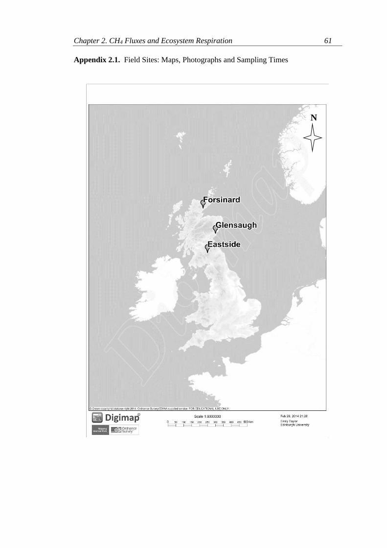
Chapter 2. CH4 Fluxes and Ecosystem Respiration 61
Appendix 2.1. Field Sites: Maps, Photographs and Sampling Times
N
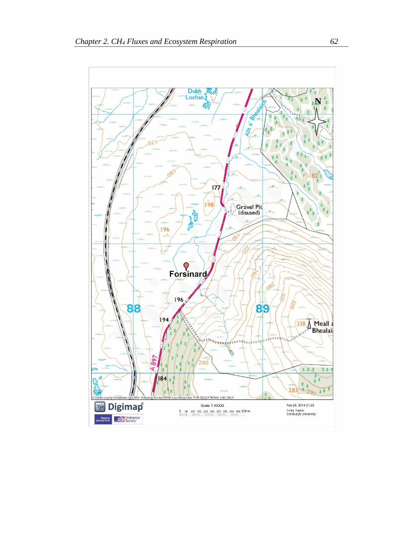
Chapter 2. CH4 Fluxes and Ecosystem Respiration 62
N
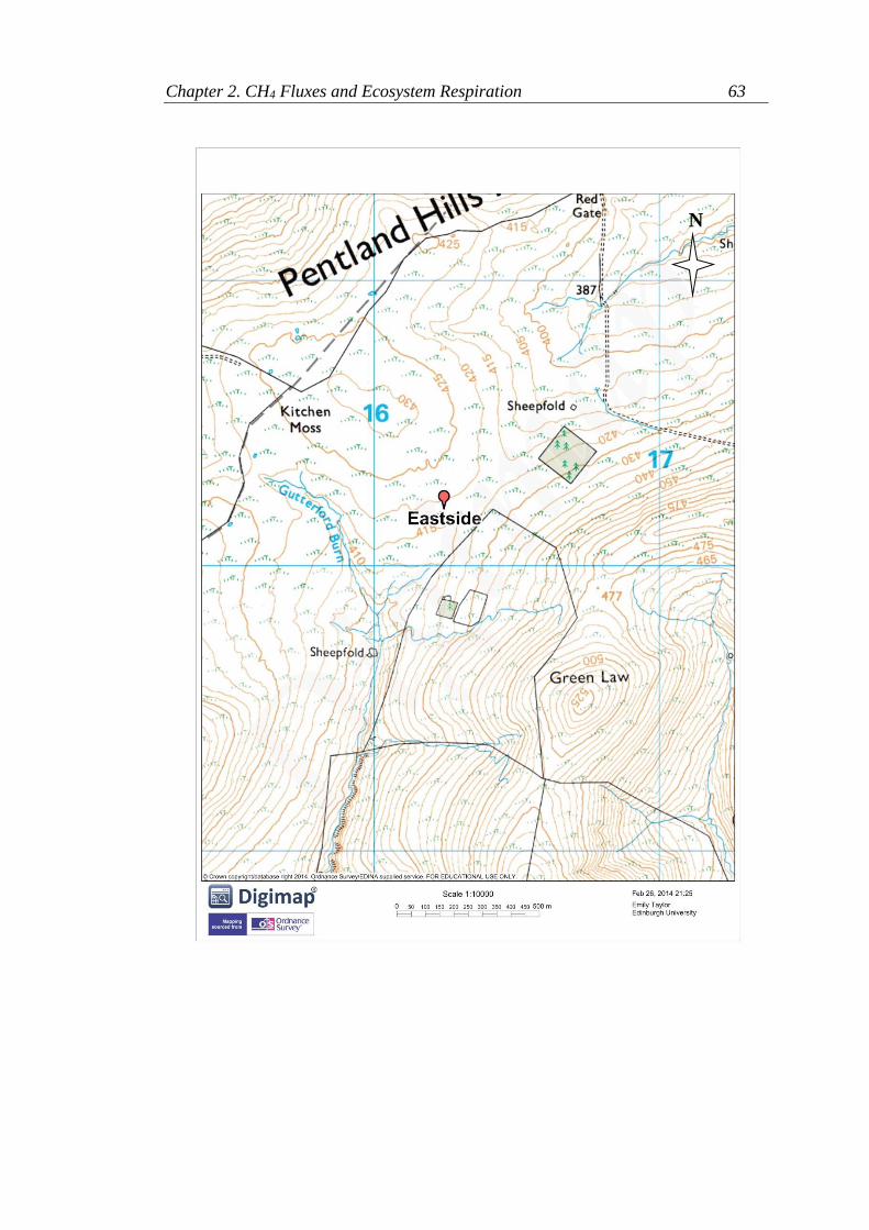
Chapter 2. CH4 Fluxes and Ecosystem Respiration 63
N
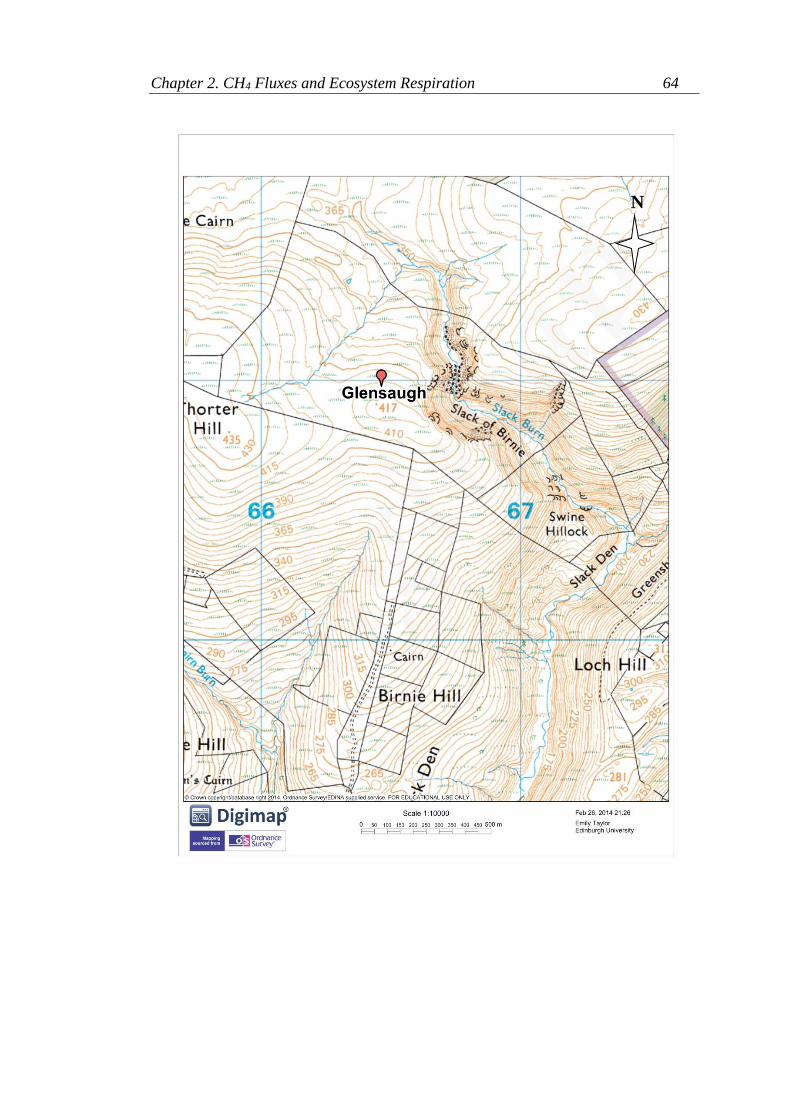
Chapter 2. CH4 Fluxes and Ecosystem Respiration 64
N
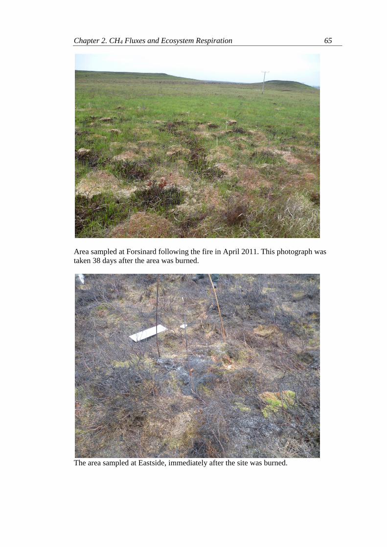
Chapter 2. CH4 Fluxes and Ecosystem Respiration 65
Area sampled at Forsinard following the fire in April 2011. This photograph was
taken 38 days after the area was burned.
The area sampled at Eastside, immediately after the site was burned.

Chapter 2. CH4 Fluxes and Ecosystem Respiration 66
The area sampled at Glensaugh 81 days after the area was burned.
Middle area shows the fire break, swiped prior to burning, with the
area to left unburnt and the area to the right the burnt area.
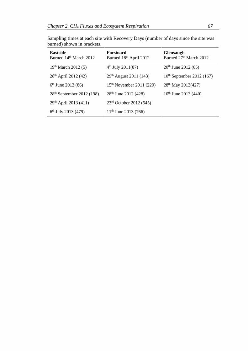
Chapter 2. CH4 Fluxes and Ecosystem Respiration 67
Sampling times at each site with Recovery Days (number of days since the site was
burned) shown in brackets.
Eastside Burned 14th March 2012
Forsinard Burned 18th April 2012
Glensaugh Burned 27th March 2012
19th March 2012 (5) 4th July 2011(87) 20th June 2012 (85)
28th April 2012 (42) 29th August 2011 (143) 10th September 2012 (167)
6th June 2012 (86) 15th November 2011 (220) 28th May 2013(427)
28th September 2012 (198) 28th June 2012 (428) 10th June 2013 (440)
29th April 2013 (411) 23rd October 2012 (545)
6th July 2013 (479) 11th June 2013 (766)

Chapter 2. CH4 Fluxes and Ecosystem Respiration 68
Appendix 2.2. Soil Temperature, Soil Moisture and Water table at the three field
sites
Soil temperature of plots at each of the three sites (E=Eastside, F=Forsinard,
G=Glensaugh) in relation to day of the year and year sites were sampled. Points
show mean with ±StEM error bars. No statistical differences were found between
burnt and unburnt plots.
4
6
8
10
12
14
4
6
8
10
12
14
4
6
8
10
12
14
EF
G
100 150 200 250 300
Julian Day
Soil
Tem
pera
ture
(C
)
Treatment
B
UB
Year
2011
2012
2013

Chapter 2. CH4 Fluxes and Ecosystem Respiration 69
Distance from surface (defined as peat/Sphagnum interface) to water table at each
plot at the two sites where dipwells were installed of the three sites (E=Eastside,
F=Forsinard) in relation to day of the year and year sites were sampled. Points show
mean with ±StEM error bars. No statistical differences were found between burnt
and unburnt plots.
-15
-10
-5
-15
-10
-5
EF
100 150 200 250 300
Julian Day
Wate
rtable
Dis
tance f
rom
Surf
ace (
cm
)
Treatment
B
UB
Year
2011
2012
2013
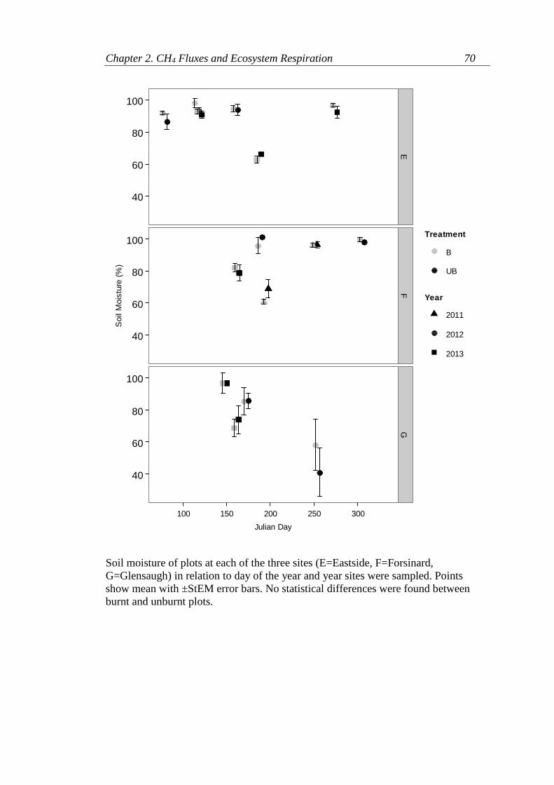
Chapter 2. CH4 Fluxes and Ecosystem Respiration 70
Soil moisture of plots at each of the three sites (E=Eastside, F=Forsinard,
G=Glensaugh) in relation to day of the year and year sites were sampled. Points
show mean with ±StEM error bars. No statistical differences were found between
burnt and unburnt plots.
40
60
80
100
40
60
80
100
40
60
80
100
EF
G
100 150 200 250 300
Julian Day
Soil
Mois
ture
(%
)
Treatment
B
UB
Year
2011
2012
2013

Chapter 2. CH4 Fluxes and Ecosystem Respiration 71
Soil moisture in relation to depth of the water table (distance the peat surface) in
plots at Forsinard and Eastside plotted with linear regression line. Regression
equation was subsequently used to estimate water table height at Glensaugh where
no dipwells were installed.
y 102 1.8 x , r2
= 0.536y 102 1.8 x , r2
= 0.536y 102 1.8 x , r2
= 0.536y 102 1.8 x , r2
= 0.536y 102 1.8 x , r2
= 0.536y 102 1.8 x , r2
= 0.536y 102 1.8 x , r2
= 0.536y 102 1.8 x , r2
= 0.536y 102 1.8 x , r2
= 0.536y 102 1.8 x , r2
= 0.536y 102 1.8 x , r2
= 0.536y 102 1.8 x , r2
= 0.536y 102 1.8 x , r2
= 0.536y 102 1.8 x , r2
= 0.536y 102 1.8 x , r2
= 0.536y 102 1.8 x , r2
= 0.536y 102 1.8 x , r2
= 0.536y 102 1.8 x , r2
= 0.536y 102 1.8 x , r2
= 0.536y 102 1.8 x , r2
= 0.536y 102 1.8 x , r2
= 0.536y 102 1.8 x , r2
= 0.536y 102 1.8 x , r2
= 0.536y 102 1.8 x , r2
= 0.536y 102 1.8 x , r2
= 0.536y 102 1.8 x , r2
= 0.536y 102 1.8 x , r2
= 0.536y 102 1.8 x , r2
= 0.536y 102 1.8 x , r2
= 0.536y 102 1.8 x , r2
= 0.536y 102 1.8 x , r2
= 0.536y 102 1.8 x , r2
= 0.536y 102 1.8 x , r2
= 0.536y 102 1.8 x , r2
= 0.536y 102 1.8 x , r2
= 0.536y 102 1.8 x , r2
= 0.536y 102 1.8 x , r2
= 0.536y 102 1.8 x , r2
= 0.536y 102 1.8 x , r2
= 0.536y 102 1.8 x , r2
= 0.536y 102 1.8 x , r2
= 0.536y 102 1.8 x , r2
= 0.536y 102 1.8 x , r2
= 0.536y 102 1.8 x , r2
= 0.536y 102 1.8 x , r2
= 0.536y 102 1.8 x , r2
= 0.536y 102 1.8 x , r2
= 0.536y 102 1.8 x , r2
= 0.536y 102 1.8 x , r2
= 0.536y 102 1.8 x , r2
= 0.536y 102 1.8 x , r2
= 0.536y 102 1.8 x , r2
= 0.536y 102 1.8 x , r2
= 0.536y 102 1.8 x , r2
= 0.536y 102 1.8 x , r2
= 0.536y 102 1.8 x , r2
= 0.536y 102 1.8 x , r2
= 0.536y 102 1.8 x , r2
= 0.536y 102 1.8 x , r2
= 0.536y 102 1.8 x , r2
= 0.536y 102 1.8 x , r2
= 0.536y 102 1.8 x , r2
= 0.536y 102 1.8 x , r2
= 0.536y 102 1.8 x , r2
= 0.536y 102 1.8 x , r2
= 0.536y 102 1.8 x , r2
= 0.536y 102 1.8 x , r2
= 0.536y 102 1.8 x , r2
= 0.536y 102 1.8 x , r2
= 0.536y 102 1.8 x , r2
= 0.536y 102 1.8 x , r2
= 0.536y 102 1.8 x , r2
= 0.536y 102 1.8 x , r2
= 0.536y 102 1.8 x , r2
= 0.536y 102 1.8 x , r2
= 0.536y 102 1.8 x , r2
= 0.536y 102 1.8 x , r2
= 0.536y 102 1.8 x , r2
= 0.536y 102 1.8 x , r2
= 0.536y 102 1.8 x , r2
= 0.536y 102 1.8 x , r2
= 0.536y 102 1.8 x , r2
= 0.536y 102 1.8 x , r2
= 0.536y 102 1.8 x , r2
= 0.536y 102 1.8 x , r2
= 0.536y 102 1.8 x , r2
= 0.536y 102 1.8 x , r2
= 0.536y 102 1.8 x , r2
= 0.536y 102 1.8 x , r2
= 0.536y 102 1.8 x , r2
= 0.536y 102 1.8 x , r2
= 0.536y 102 1.8 x , r2
= 0.536y 102 1.8 x , r2
= 0.536y 102 1.8 x , r2
= 0.536y 102 1.8 x , r2
= 0.536y 102 1.8 x , r2
= 0.536y 102 1.8 x , r2
= 0.536y 102 1.8 x , r2
= 0.536y 102 1.8 x , r2
= 0.536y 102 1.8 x , r2
= 0.536y 102 1.8 x , r2
= 0.536y 102 1.8 x , r2
= 0.536y 102 1.8 x , r2
= 0.536y 102 1.8 x , r2
= 0.536y 102 1.8 x , r2
= 0.536y 102 1.8 x , r2
= 0.536y 102 1.8 x , r2
= 0.536y 102 1.8 x , r2
= 0.536y 102 1.8 x , r2
= 0.536y 102 1.8 x , r2
= 0.536y 102 1.8 x , r2
= 0.536y 102 1.8 x , r2
= 0.536y 102 1.8 x , r2
= 0.536y 102 1.8 x , r2
= 0.536y 102 1.8 x , r2
= 0.536y 102 1.8 x , r2
= 0.536y 102 1.8 x , r2
= 0.536y 102 1.8 x , r2
= 0.536y 102 1.8 x , r2
= 0.536y 102 1.8 x , r2
= 0.536y 102 1.8 x , r2
= 0.536y 102 1.8 x , r2
= 0.536y 102 1.8 x , r2
= 0.536y 102 1.8 x , r2
= 0.536y 102 1.8 x , r2
= 0.536y 102 1.8 x , r2
= 0.536y 102 1.8 x , r2
= 0.536y 102 1.8 x , r2
= 0.536y 102 1.8 x , r2
= 0.536y 102 1.8 x , r2
= 0.536y 102 1.8 x , r2
= 0.536y 102 1.8 x , r2
= 0.536y 102 1.8 x , r2
= 0.536y 102 1.8 x , r2
= 0.536y 102 1.8 x , r2
= 0.536y 102 1.8 x , r2
= 0.536y 102 1.8 x , r2
= 0.536y 102 1.8 x , r2
= 0.536y 102 1.8 x , r2
= 0.536y 102 1.8 x , r2
= 0.536y 102 1.8 x , r2
= 0.536y 102 1.8 x , r2
= 0.536y 102 1.8 x , r2
= 0.536y 102 1.8 x , r2
= 0.536y 102 1.8 x , r2
= 0.536y 102 1.8 x , r2
= 0.536y 102 1.8 x , r2
= 0.536y 102 1.8 x , r2
= 0.536y 102 1.8 x , r2
= 0.536y 102 1.8 x , r2
= 0.536y 102 1.8 x , r2
= 0.536y 102 1.8 x , r2
= 0.536y 102 1.8 x , r2
= 0.536y 102 1.8 x , r2
= 0.536y 102 1.8 x , r2
= 0.536y 102 1.8 x , r2
= 0.536y 102 1.8 x , r2
= 0.536y 102 1.8 x , r2
= 0.536y 102 1.8 x , r2
= 0.536y 102 1.8 x , r2
= 0.536y 102 1.8 x , r2
= 0.536y 102 1.8 x , r2
= 0.536y 102 1.8 x , r2
= 0.536y 102 1.8 x , r2
= 0.536y 102 1.8 x , r2
= 0.536y 102 1.8 x , r2
= 0.536y 102 1.8 x , r2
= 0.536y 102 1.8 x , r2
= 0.536y 102 1.8 x , r2
= 0.536y 102 1.8 x , r2
= 0.536y 102 1.8 x , r2
= 0.536y 102 1.8 x , r2
= 0.536y 102 1.8 x , r2
= 0.536y 102 1.8 x , r2
= 0.536y 102 1.8 x , r2
= 0.536y 102 1.8 x , r2
= 0.536y 102 1.8 x , r2
= 0.536y 102 1.8 x , r2
= 0.536y 102 1.8 x , r2
= 0.536y 102 1.8 x , r2
= 0.536y 102 1.8 x , r2
= 0.536y 102 1.8 x , r2
= 0.536y 102 1.8 x , r2
= 0.536y 102 1.8 x , r2
= 0.536y 102 1.8 x , r2
= 0.536y 102 1.8 x , r2
= 0.536y 102 1.8 x , r2
= 0.536y 102 1.8 x , r2
= 0.536y 102 1.8 x , r2
= 0.536y 102 1.8 x , r2
= 0.536y 102 1.8 x , r2
= 0.536y 102 1.8 x , r2
= 0.536y 102 1.8 x , r2
= 0.536y 102 1.8 x , r2
= 0.536y 102 1.8 x , r2
= 0.536y 102 1.8 x , r2
= 0.536y 102 1.8 x , r2
= 0.536y 102 1.8 x , r2
= 0.536y 102 1.8 x , r2
= 0.536y 102 1.8 x , r2
= 0.536y 102 1.8 x , r2
= 0.536y 102 1.8 x , r2
= 0.536y 102 1.8 x , r2
= 0.536y 102 1.8 x , r2
= 0.536y 102 1.8 x , r2
= 0.536y 102 1.8 x , r2
= 0.536y 102 1.8 x , r2
= 0.536y 102 1.8 x , r2
= 0.536y 102 1.8 x , r2
= 0.536y 102 1.8 x , r2
= 0.536y 102 1.8 x , r2
= 0.536y 102 1.8 x , r2
= 0.536y 102 1.8 x , r2
= 0.536y 102 1.8 x , r2
= 0.536y 102 1.8 x , r2
= 0.536y 102 1.8 x , r2
= 0.536y 102 1.8 x , r2
= 0.536y 102 1.8 x , r2
= 0.536y 102 1.8 x , r2
= 0.536y 102 1.8 x , r2
= 0.536y 102 1.8 x , r2
= 0.536y 102 1.8 x , r2
= 0.536y 102 1.8 x , r2
= 0.536y 102 1.8 x , r2
= 0.536y 102 1.8 x , r2
= 0.536y 102 1.8 x , r2
= 0.536y 102 1.8 x , r2
= 0.536y 102 1.8 x , r2
= 0.536y 102 1.8 x , r2
= 0.536y 102 1.8 x , r2
= 0.536y 102 1.8 x , r2
= 0.536y 102 1.8 x , r2
= 0.536y 102 1.8 x , r2
= 0.536y 102 1.8 x , r2
= 0.536y 102 1.8 x , r2
= 0.536y 102 1.8 x , r2
= 0.536y 102 1.8 x , r2
= 0.536y 102 1.8 x , r2
= 0.536y 102 1.8 x , r2
= 0.536y 102 1.8 x , r2
= 0.536y 102 1.8 x , r2
= 0.536y 102 1.8 x , r2
= 0.536y 102 1.8 x , r2
= 0.536y 102 1.8 x , r2
= 0.536y 102 1.8 x , r2
= 0.536y 102 1.8 x , r2
= 0.536y 102 1.8 x , r2
= 0.536y 102 1.8 x , r2
= 0.536y 102 1.8 x , r2
= 0.536y 102 1.8 x , r2
= 0.536y 102 1.8 x , r2
= 0.536y 102 1.8 x , r2
= 0.536y 102 1.8 x , r2
= 0.536y 102 1.8 x , r2
= 0.536y 102 1.8 x , r2
= 0.536y 102 1.8 x , r2
= 0.536y 102 1.8 x , r2
= 0.536y 102 1.8 x , r2
= 0.536y 102 1.8 x , r2
= 0.536y 102 1.8 x , r2
= 0.536y 102 1.8 x , r2
= 0.536y 102 1.8 x , r2
= 0.536y 102 1.8 x , r2
= 0.536y 102 1.8 x , r2
= 0.536y 102 1.8 x , r2
= 0.536y 102 1.8 x , r2
= 0.536y 102 1.8 x , r2
= 0.536y 102 1.8 x , r2
= 0.536y 102 1.8 x , r2
= 0.536y 102 1.8 x , r2
= 0.536y 102 1.8 x , r2
= 0.536y 102 1.8 x , r2
= 0.536y 102 1.8 x , r2
= 0.536y 102 1.8 x , r2
= 0.536y 102 1.8 x , r2
= 0.536y 102 1.8 x , r2
= 0.536y 102 1.8 x , r2
= 0.536y 102 1.8 x , r2
= 0.536y 102 1.8 x , r2
= 0.536y 102 1.8 x , r2
= 0.536y 102 1.8 x , r2
= 0.536y 102 1.8 x , r2
= 0.536y 102 1.8 x , r2
= 0.536y 102 1.8 x , r2
= 0.536y 102 1.8 x , r2
= 0.536y 102 1.8 x , r2
= 0.536y 102 1.8 x , r2
= 0.536y 102 1.8 x , r2
= 0.536y 102 1.8 x , r2
= 0.536y 102 1.8 x , r2
= 0.536y 102 1.8 x , r2
= 0.536y 102 1.8 x , r2
= 0.536y 102 1.8 x , r2
= 0.536y 102 1.8 x , r2
= 0.536y 102 1.8 x , r2
= 0.536y 102 1.8 x , r2
= 0.536y 102 1.8 x , r2
= 0.536y 102 1.8 x , r2
= 0.536y 102 1.8 x , r2
= 0.536y 102 1.8 x , r2
= 0.536y 102 1.8 x , r2
= 0.536y 102 1.8 x , r2
= 0.536y 102 1.8 x , r2
= 0.536y 102 1.8 x , r2
= 0.536y 102 1.8 x , r2
= 0.536y 102 1.8 x , r2
= 0.536y 102 1.8 x , r2
= 0.536y 102 1.8 x , r2
= 0.536y 102 1.8 x , r2
= 0.536y 102 1.8 x , r2
= 0.536y 102 1.8 x , r2
= 0.536y 102 1.8 x , r2
= 0.536y 102 1.8 x , r2
= 0.536y 102 1.8 x , r2
= 0.536y 102 1.8 x , r2
= 0.536y 102 1.8 x , r2
= 0.536y 102 1.8 x , r2
= 0.536y 102 1.8 x , r2
= 0.536y 102 1.8 x , r2
= 0.536y 102 1.8 x , r2
= 0.536y 102 1.8 x , r2
= 0.536y 102 1.8 x , r2
= 0.536y 102 1.8 x , r2
= 0.536y 102 1.8 x , r2
= 0.536y 102 1.8 x , r2
= 0.536y 102 1.8 x , r2
= 0.536y 102 1.8 x , r2
= 0.536y 102 1.8 x , r2
= 0.536y 102 1.8 x , r2
= 0.536y 102 1.8 x , r2
= 0.536y 102 1.8 x , r2
= 0.536y 102 1.8 x , r2
= 0.536y 102 1.8 x , r2
= 0.536y 102 1.8 x , r2
= 0.536y 102 1.8 x , r2
= 0.536y 102 1.8 x , r2
= 0.536y 102 1.8 x , r2
= 0.536y 102 1.8 x , r2
= 0.536y 102 1.8 x , r2
= 0.536y 102 1.8 x , r2
= 0.536y 102 1.8 x , r2
= 0.536y 102 1.8 x , r2
= 0.536y 102 1.8 x , r2
= 0.536y 102 1.8 x , r2
= 0.536y 102 1.8 x , r2
= 0.536y 102 1.8 x , r2
= 0.536y 102 1.8 x , r2
= 0.536y 102 1.8 x , r2
= 0.536y 102 1.8 x , r2
= 0.536y 102 1.8 x , r2
= 0.536y 102 1.8 x , r2
= 0.536y 102 1.8 x , r2
= 0.536y 102 1.8 x , r2
= 0.536y 102 1.8 x , r2
= 0.536y 102 1.8 x , r2
= 0.536y 102 1.8 x , r2
= 0.536y 102 1.8 x , r2
= 0.536y 102 1.8 x , r2
= 0.536y 102 1.8 x , r2
= 0.536y 102 1.8 x , r2
= 0.536y 102 1.8 x , r2
= 0.536y 102 1.8 x , r2
= 0.536y 102 1.8 x , r2
= 0.536y 102 1.8 x , r2
= 0.536y 102 1.8 x , r2
= 0.536y 102 1.8 x , r2
= 0.536y 102 1.8 x , r2
= 0.536y 102 1.8 x , r2
= 0.53630
60
90
-20 -15 -10 -5 0
Watertable depth from surface (cm)
Soil
Mois
ture
(%
)
Site
E
F
G
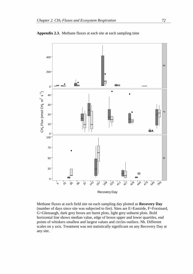
Chapter 2. CH4 Fluxes and Ecosystem Respiration 72
Appendix 2.3. Methane fluxes at each site at each sampling time
Methane fluxes at each field site on each sampling day plotted as Recovery Day
(number of days since site was subjected to fire). Sites are E=Eastside, F=Forsinard,
G=Glensaugh, dark grey boxes are burnt plots, light grey unburnt plots. Bold
horizontal line shows median value, edge of boxes upper and lower quartiles, end
points of whiskers smallest and largest values and circles outliers. Nb. Different
scales on y axis. Treatment was not statistically significant on any Recovery Day at
any site.
0
200
400
0
10
20
30
40
0
25
50
75
100
EF
G
5 42 85 86 87 143
167
198
220
411
427
428
440
479
545
766
Recovery Day
CH
4 F
lux
(n
mo
l C
H4 m
2 s
1)
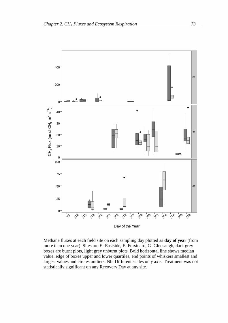
Chapter 2. CH4 Fluxes and Ecosystem Respiration 73
Methane fluxes at each field site on each sampling day plotted as day of year (from
more than one year). Sites are E=Eastside, F=Forsinard, G=Glensaugh, dark grey
boxes are burnt plots, light grey unburnt plots. Bold horizontal line shows median
value, edge of boxes upper and lower quartiles, end points of whiskers smallest and
largest values and circles outliers. Nb. Different scales on y axis. Treatment was not
statistically significant on any Recovery Day at any site.
0
200
400
0
10
20
30
40
0
25
50
75
100
EF
G
79 116
119
148
160
161
162
172
187
188
195
251
254
274
305
328
Day of the Year
CH
4 F
lux
(n
mo
l C
H4 m
2 s
1)
Post-burn
Day 4

Chapter 2. CH4 Fluxes and Ecosystem Respiration 74
Appendix 2.4. Ecosystem Respiration at each site at each sampling time
Ecosystem Respiration at each field site on each sampling day plotted as Recovery
Day (number of days since site was subjected to fire). Sites are E=Eastside,
F=Forsinard, G=Glensaugh, dark grey boxes are burnt plots, light grey unburnt plots.
Bold horizontal line shows median value, edge of boxes upper and lower quartiles,
end points of whiskers smallest and largest values and circles outliers. Asterisk show
where there was a significant difference between burnt and unburnt treatments
(*indicates where p<0.05, ** p<0.01, ***p<0.001). Nb. Different scales on y axis.
0
1000
2000
0
1000
2000
3000
4000
2000
4000
6000
EF
G
5 42 85 86 87 143
167
198
220
411
427
428
440
479
545
766
Recovery Day
ER
(n
mo
l C
O2 m
2 s
1)
***
*
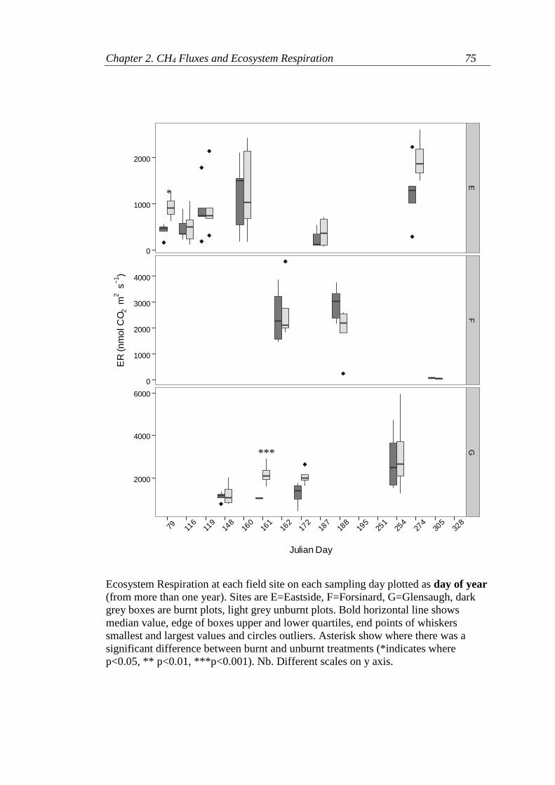
Chapter 2. CH4 Fluxes and Ecosystem Respiration 75
Ecosystem Respiration at each field site on each sampling day plotted as day of year
(from more than one year). Sites are E=Eastside, F=Forsinard, G=Glensaugh, dark
grey boxes are burnt plots, light grey unburnt plots. Bold horizontal line shows
median value, edge of boxes upper and lower quartiles, end points of whiskers
smallest and largest values and circles outliers. Asterisk show where there was a
significant difference between burnt and unburnt treatments (*indicates where
p<0.05, ** p<0.01, ***p<0.001). Nb. Different scales on y axis.
0
1000
2000
0
1000
2000
3000
4000
2000
4000
6000
EF
G
79 116
119
148
160
161
162
172
187
188
195
251
254
274
305
328
Julian Day
ER
(n
mo
l C
O2 m
2 s
1)
*
***

Chapter 3. Recovery of Sphagnum capillifolium 76
3. The recovery of Sphagnum capillifolium following exposure to
temperatures of simulated moorland fires: a glasshouse experiment
3.1 Abstract
In the UK blanket bog can be burnt by wildfires and deliberately for
management purposes under government legislation and guidelines. Sphagnum
mosses are considered a key component of a blanket bog system so their response to
fire is important to understand for the formulation best practice burning guidance.
Previous research on peatland fires has shown that the moss layer can be subjected to
high, potentially physiologically damaging, temperatures and that frequent burning
can lead to a decline in bryophyte cover. To date however there is no empirical
evidence for the short term effects of fire on Sphagnum. Here we show that
Sphagnum capillifolium has the ability to recover from exposure to high temperatures
analogous to those previously recorded in managed peatland fires. We found that
recovery of S.capillifolium as indicated by chlorophyll fluorescence, net primary
productivity and new growth was related temperatures experienced at the Sphagnum
layer surface, post-fire environmental conditions and pre-burn stem moisture content.
The lowest rates of photosynthetic recovery were found when samples were heated
to 400oC for 30 seconds with the lowest rates of photosynthesis and new auxiliary
growth during winter months. Our results demonstrate there are situations conducive
to S.capillifolium recovery following a fire and that spring fires may allow for
quicker recovery. We anticipate our results will help inform burning regimes that aim
to do least damage to the Sphagnum layer. In addition the results provide important

Chapter 3. Recovery of Sphagnum capillifolium 77
evidence that seasonality and post-burn conditions should be considered when
formulating assessments of the short term impacts of a fire on the Sphagnum layer.
3.2 Introduction
Sphagnum mosses are often considered the foundation or building block of
ombrotrophic boreal peatlands (Rydin and Jeglum, 2006) and have unique
capabilities which allow them to survive in the nutrient poor and acidic peatland
environment. They can be considered ‘ecosystem engineers’ (Jones et al., 1994) in
the sense that the physical conditions they thrive in are in part determined and
maintained by the plants themselves (Clymo and Hayward, 1982). Their water
holding capacity, both internally within cells and externally due to their morphology,
help maintain the wet and anoxic conditions of a peatland, while reducing the risk
and amplitude of desiccation of their photosynthetically active capitulum (Hayward
and Clymo, 1982). Sphagnum also produce the organic acids responsible for both
creating and maintaining the acidic conditions of ombrotrophic and minerotropic
boreal peatlands (Kuhry et al., 1993) and have the ability to lock away nutrients
making them unavailable to other species (Rydin and Jeglum, 2006), important
factors in creating the unique environmental conditions and associated fauna and
flora. The recalcitrant nature of Sphagnum, thought to be due to the intercellular
concentrations of phenolic compounds and uronic acids (Børsheim et al., 2001), also
means it is very resistant to decay and is likely the most important component for
peat formation worldwide (Malmer and Wallén, 2004). It is therefore important to
understand the impact disturbance events may have on the Sphagnum layer,
especially now when greater emphasis is given to maintaining peatlands as long term
Chapter 3. Recovery of Sphagnum capillifolium 78
carbon stores. Furthermore Sphagnum species are significant components of habitats
of conservation concern, with both active raised and blanket bog and transition mires
and quaking bogs European Habitat Directive Annex I habitats. Active raised and
blanket bogs are priority habitats, and the UK has special responsibility for their
protection and so are often interest features of Special Areas of Conservation (SAC).
At an individual species level some species are particularly vulnerable in the UK,
with one species, Sphagnum obtusum Warnst., thought to have gone extinct during
the 20th Century, with Sphagnum balticum (Russow) C.E.O.Jensen. and Sphagnum
skyense Flatberg. classed as endangered and near threatened respectively. One such
disturbance event which could have consequences for Sphagnum is fire, which could
have both direct and indirect effects on the Sphagnum layer as a whole and at an
individual species level.
In the UK peatlands, as well as being potentially burnt by wildfire, can be
burned legally following guidance set out in the Muirburn Code in Scotland and the
Heather and Grass Burning 2007 Code in England. In Scotland, management burning
specifically on blanket bog can only occur during the muirburn season when heather
(Calluna vulgaris) constitutes more than 75% of the vegetation cover while in
England can only be burned as part of a pre-approved burning plan for conservation
and restoration with the aim of not damaging the moss layer (Department for
Environment Food and Rural Affairs, 2007, Scottish Executive, 2011). This makes
understanding the response of Sphagnum species, such an important component of a
blanket bog, important if damage to Sphagnum by burning is to be limited. To date,

Chapter 3. Recovery of Sphagnum capillifolium 79
however, little direct research has looked at the direct effect fire has on the
Sphagnum layer as a whole or at an individual species level in peatlands.
Studies looking at the characteristics of fires on peatlands have shown that
although the bryophyte layer can be exposed to high temperatures, these
temperatures are usually not as high as those found in the canopy vegetation (eg.
Hobbs and Gimingham, 1984, Hamilton, 2000, Davies, 2005). In fires over Calluna
vulgaris (L.) Hull (here after referred to as Calluna) dominated heaths it has been
demonstrated that temperatures rarely exceed 50oC 2cm below the surface of
pleurocarpous mosses (Davies, 2005). However, temperatures lethal for bryophytes
by which cell damage occurs are thought to be between 40 and 51 oC (Glime, 2007)
so even temperatures significantly lower than those found in the canopy vegetation
may still be physiologically damaging. At the ground/moss surface temperatures can
be significantly higher, up to 600oC, even if for relatively short (<30 seconds)
periods of time (Davies, 2005, Hamilton, 2000). Such high surface temperatures
could have an impact on Sphagnum growth particularly by damaging the capitulum,
wherein the apical meristem and the site of the majority of photosynthesis resides
(Rydin and Jeglum, 2006). However, as Sphagnum typically grows in vertical shoots
it is possible that when fire only damages the capitulum and upper sections of stems
Sphagnum could have the ability to re-grow from side shoots (Rydin and Jeglum,
2006) meaning recovery may be possible, which has indeed been observed in certain
circumstances in the field (Hamilton, 2000). There are however instances when high
temperatures may penetrate much deeper into the moss layer and peat, when the peat
itself ignites and smoulders (Ashton et al., 2007). This may be a result of the

Chapter 3. Recovery of Sphagnum capillifolium 80
structure and distribution of fuel above the moss layer, with a high density of fuel
increasing the temperature residence time within a fire in a confined area, causing
greater evaporation and so lowering the moisture content of the vegetation and peat
and allowing the fire to penetrate the peat. Such “hot spots” have been observed in
Calluna fires (Davies, 2005) and in the moss layer in areas immediately around the
woody stems of Calluna (Hamilton, 2000). Lab based burning experiments have
demonstrated the importance of moisture status for allowing the smouldering of
pleurocarpus mosses with a critical “fuel moisture threshold” existing at a moisture
content of around 16%. Below this threshold the moss smouldered and often flamed,
and above the threshold smouldering was slower, often self-extinguishing, and never
igniting (Legg et al., 2008). Peat below the moss layer has also been widely
demonstrated to be more likely to ignite and smoulder in wildfires when drier (eg.
Frandsen, 1997, Rein et al., 2008, Davies et al., 2013).
It is intuitive that the moisture content of the Sphagnum layer prior to burning
will have an effect on the impact of high temperatures, as higher water contents can
make vegetation less susceptible to being burned, as has been found in grasses (eg.
Lloyd, 1968) and Calluna (eg. Kayll 1966, Hamilton 2000, Davies et al., 2009). The
study by Legg et al., (2008) also showed the importance of the bulk density of the
moss layer for the probability of ignition, with low densities heated with igniters
failing to smoulder, which the authors suggests is due to the rapid vaporisation of
moss directly in contact with the igniter creating a small hollow where smouldering
could not take hold. Although low densities may not be conducive to ignition and
smouldering, low densities may increase the rate of evaporation (Titus and Wagner,

Chapter 3. Recovery of Sphagnum capillifolium 81
1984) reducing moisture content, subsequently increasing the risk of burning. In
Sphagnum the looser arrangement of hollow and lawn forming species have been
found to be more susceptible to burning than hummock forming species such as
Sphagnum fuscum (Schimp.) H.Klinggr. which are more densely arranged (Benscoter
et al., 2011). These potential short term effects of fire on the Sphagnum layer may
therefore have important repercussions for rates of recovery, primary production and
if linked to density and morphology may be species specific and therefore important
to long term species composition and succession.
Previously, a long term study at an experimental burning on blanket bog with
a fire frequency rate of 10 years found that overall bryophytes declined with burning
(Ward et al., 2007) but that Sphagnum spp. increased in abundance (Lee et al.,
2013). Little work however has looked at the specific response of different
Sphagnum species to burning, although Barkman (1992) reported differences in rates
of recovery between species on a Dutch bog, with no studies relating Sphagnum
recovery to fire characteristics and pre and post fire conditions. It is possible that fire
may favour some Sphagnum species over others as has been found at some sites in
the North York Moors where Sphagnum capillifolium (Ehrh.) Hedw. was found to be
more abundant at sites burned more recently (Burch, 2009). However, studying the
abundance and distribution of Sphagnum species in relation to fire distribution to
infer the impact fire has on Sphagnum may be too simplistic as it is possible that the
distribution of Sphagnum species may be associated more by the ecophysiology of
species. S.capillifolium for example can thrive in much drier conditions than other
Sphagnum species so is often found in areas of blanket bog that experience burning,

Chapter 3. Recovery of Sphagnum capillifolium 82
as burning is usually confined to drier areas where fire can be ignited. A more direct
and functional approach to determining the effect of fire on Sphagnum species is
therefore also needed.
3.3 Aims
The aim of this study was to quantify the recovery of S.capillifolium
following exposure to temperature treatments simulating different maximum
temperature and residency times analogous to those during Calluna fires.
S.capillifolium was chosen as it is a species often associated with Calluna dominated
heaths (Rodwell, 1991) and is a common species found in areas managed by fire
under the regulations set out in the Muirburn Code (Scottish Executive, 2011). Based
on previous research on critical temperatures in bryophytes (Glime, 2007) it was
hypothesised that: [1] the photosynthetic capacity of S. capillifolium would be
reduced following exposure to high temperatures and be more adversely affected by
higher temperatures and temperature residency times and [2] a critical temperature
and temperature residency time exists above which the temperature treatments will
be lethal to S.capillifolium.
3.4 Materials and Methods
3.4.1 Experimental Design
Sphagnum capillifolium was collected from Whim Moss, Penicuik, South
East Scotland (NT203532), an ombrotrophic blanket bog classified under the
National Vegetation Classification (NVC) as M19 Calluna vulgaris-Eriophorum
vaginatum blanket mire which lies 280m above sea level with a mean air temperature

Chapter 3. Recovery of Sphagnum capillifolium 83
(2003–2009) of 8.6oC (ranging from −9.2 to 27.7 oC) (Sheppard et al., 2012). 6cm
deep, 5cm diameter round clumps of S.capillifolium were collected a maximum of
two days prior to start of each run of the experiment from 4 different, randomly
selected, hummocks per run of the experiment, and placed into 5cm diameter round
fibre pots (Grow It, Spalding, UK). While potting, the clumps were kept as intact as
possible to ensure that the number of stems in each pot was representative of natural
stem densities found within each hummock. For each run of the experiment 96 pots
filled with S.capillifolium were placed within a tray containing a bed of
S.capillifolium cuttings, to help maintain damp conditions and simulate a more
natural habitat. For the duration of the experiment the tray kept within a glasshouse
designed to track external air temperatures to within 2oC. The surrounding Sphagnum
bedding was watered regularly and each pot watered with distilled water individually
using a syringe to maintain S.capillifolium moisture content to around 90%, the
amount of water given to each pot varying in response to stem moisture content,
which was calculated for individual stems on a dry weight basis each time
throughout each run of the experiment. During dry and hot conditions in the
glasshouse the entire tray was sprayed uniformly with distilled water up to three
times a day to ensure samples did not dry out. A pilot study (Appendix 3.1) was
conducted prior to the experiment to ensure S.capillifolium samples could remain
healthy, with plant health monitored using chlorophyll florescence measurements
which gave an indication of the photosynthetic capacity of individual stems as
discussed in section 3.4.2.1.

Chapter 3. Recovery of Sphagnum capillifolium 84
The experiment was run three times with one of three different temperature
treatments randomly assigned to each of the 96 pots per run (Table 3. 1). Each pot
was also assigned randomly to one of 4 measurement procedures; chlorophyll
fluorescence, CO2 exchange, growth measurements and moisture content analysis.
Multiple measurements could not be made on each pot as both the chlorophyll
fluorescence and moisture content analysis were destructive (Appendix 3.2).

Table 3. 1 Temperature treatments used for each of the three runs of the experiment. Burn Season refers to the time of year the pots
were exposed to each burn treatment. All pots were observed and recovery measurements made for a total of 100 days after being
exposed to each temperature treatment which is termed Observation Period in the table. *400+D indicates where the treatment was
carried out on pots of S.capillifolium subjected to three days of drying prior to the treatment.
Run
Simulated
Burn
Season
Observation
Period
Treatment
Name
Maximum
Surface
Temp
(oC)
Maximum
Temperature
Residence Time
at Surface
(s)
Mean Sphagnum
Moisture
Content when
burnt (%
wet weight basis)
1 Spring Mar‘12 – Jun’12 Control Ambient (~9oC) -
100 100 3s at max surface temp 89.5
400 400 3s at max surface temp 89.6
2 Autumn Oct’12 – Jan’13 Control Ambient (~16oC) -
400 400 3s at max surface temp 89.6
400+ 400 30s between 350 &
450oC
92.5
3 Winter Feb’13 – May’13 Control Ambient (~3oC) -
400+ 400 30s between 350 &
450oC
92.5
400+D* 400 30s between 350 &
450oC
80.6
Chapter 3
. Reco
very of S
phagnum
capillifo
lium
85
Chapter 3. Recovery of Sphagnum capillifolium 86
The temperature treatments were performed by placing each individual pot in
a perforated steel heating chamber, which was heated by a butane-propane flame
from a weed wand (Parasene Weed Wand 550, Parasene, UK). The flame was held in
place until the surface of the pot of Sphagnum within the chamber reached the
desired maximum temperature for the desired length of time. The perforated steel
chamber was used to limit the consumption and charring of the whole pot as a
consequence of being heated by a direct flame burning with a temperature of around
1000oC. Temperature measurements logged every 2 seconds using k-type twisted
thermocouple wire connected to a datalogger (CR21X, Campbell Scientific, Utah,
USA). Thermocouples were places at the surface and at 2cm and 5cm depth within
the pots. The surface temperature (displayed in real time on the data logger screen)
was used to determine when to remove the flame to meet the desired temperature
conditions of each treatment. The temperature treatments were designed to simulate
temperatures and temperature residency conditions that have been recorded at the
moss surface within Calluna fires on heaths in Scotland (Davies per comn. 2010).
Due to the method of heating there was some variation around the maximum
temperatures and maximum temperature residency times but each treatment did give
distinctly different temperature conditions (Appendix 3.3). The 400+D treatment also
involved drying the Sphagnum prior to burning by not watering the pots and keeping
them in a separate tray without a bed of damp Sphagnum cuttings, surrounded by 6
small battery powered fans and kept at an air temperature of 18oC for three days (all
other treatments were potted into damp fibre pots and placed immediately into the
tray of Sphagnum cuttings with no fans). Post-burn, the 400+D pots were placed with

Chapter 3. Recovery of Sphagnum capillifolium 87
the others in the damp tray of Sphagnum cuttings and watered as per the others to
maintain stem moisture content of around 90% (wet weight basis). Sphagnum stems
were removed from pots assigned to each treatment through each run of the
experiment for moisture content analysis (Appendix 3.4). The mean, minimum and
maximum air temperature and light intensity (PAR) for each day of each run of the
experiment were calculated from external ambient PAR and temperatures calibrated
with actual measurements taken within the glasshouse over a period of weeks where
internal measurements were available (Appendix 3.4).
3.4.2 Recovery Measurements
3.4.2.1 Chlorophyll Fluorescence
Chlorophyll fluorescence is a well established technique for measuring plant
stress (Krause and Weis, 1991, Maxwell and Johnson, 2000) and has been
demonstrated as a reliable method for evaluating stress and recovery in Sphagnum
(eg. Manninen et al., 2011, van Gaalen et al., 2007, Hájek and Beckett, 2008). The
technique works on the principle that, when damaged, Photosystem II (PS II) re-
emits more energy when exposed to light as less is absorbed by chlorophyll for use in
the photochemical process (Maxwell and Johnson, 2000). This energy, fluorescence,
can then be measured as the variable florescence (Fv) which is the maximal
florescence (Fm) when saturated with light, minus minimum florescence (Fo) when
first exposed to light, with the ratio Fv/Fm, described as the maximum quantum yield
of PSII, indicative of stress (Maxwell and Johnson, 2000). An Fv/Fm ratio of 0.75 to
0.84 is the widely accepted range expected in healthy vascular plants (Demmig and

Chapter 3. Recovery of Sphagnum capillifolium 88
Björkman, 1987) and mosses (eg. Bates et al., 2009, Hájek and Beckett, 2008, Green
et al., 1998, Manninen et al., 2011, Proctor, 2003, van Gaalen et al., 2007).
Chlorophyll fluorescence measurements were made using a Continuous
Excitation Chlorophyll Fluorimeter (HandyPEA, Hansatech Instruments Ltd, UK) on
the capitulum of one stem from each individual pot assigned to the fluorescence
measurement protocol for each treatment on 8 separate days starting from the first
day after being exposed to the temperature treatments up to 100 days after exposure
to the temperature treatments. Each capitulum was dark adapted for 20 minutes using
a dark adaption clip (HPEA/LC, Hansatech Instruments Ltd, UK) prior to making the
measurement at a light intensity of 1500 µmol m-2 s-1 (Carfrae, 2005). Concurrently a
stem was removed from another 8 individual pots per treatment for moisture content
analysis to ensure the Sphagnum samples were maintaining healthy moisture content
of around 90% (wet weight basis). Chlorophyll fluorescence was also used to assess
physiological damage from the capitulum downwards along a stem by making
measurements at 5 mm intervals down a sub-sample of stems taken from pots from
each treatment in Run2 at 100 days when pots were harvested.
3.4.2.2 CO2 Exchange
Gas exchange measurements were made on 8 pots per treatment on 5
occasions from day 3 to day 99 of each run of the experiment. Measurements were
made using a portable infra-red gas analyser (LI-6400XT, Li-Cor, Lincoln, NE,
USA) with a purposely designed sample chamber to measure net primary
productivity (NPP) of the whole pots of Sphagnum. Prior to embarking on the

Chapter 3. Recovery of Sphagnum capillifolium 89
experiment, gas exchange measurements were made on the empty fibre plant pots
used to hold the Sphagnum samples. Results of these tests showed that, particularly
when wet, these pots did respire, increasing CO2 concentrations in the sample
chamber. Therefore, throughout each run of the experiment each pot of Sphagnum
was carefully decanted into an inert plastic pot of the same size for the gas exchange
measurements. After each measurement was made the samples were returned to their
original peat pots. The sample chamber was connected to a flow meter (6400-18
RGB, Li-Cor, Lincoln, NE, USA) which contained silica gel beads to reduce
humidity in the sample chamber. It was found that a method to reduce humidity in
the chamber, caused by the high moisture content of the Sphagnum samples in
comparison to plants the system was designed for, was vital for maintaining accuracy
and to stop condensation on the infra-red gas analysers. The Licor LI-6400XT was
set to maintain the sample chamber air temperature at 20oC with an initial 400μmol
of CO2 with a flow rate to the sample chamber of 500 μmol s-1. This temperature
condition was chosen as it was the most maintainable in lab conditions throughout
each run of the experiment. The light source used was a 6400-18 RGB (Licor,
Lincoln, NE, USA) with NPP measured under a white light intensity of 2000μmol m2
s-1, to give the highest rates of CO2 assimilation (Appendix 3.5), and respiration
under a light intensity of <1μmol m2 s-1. NPP, measured in all three runs of the
experiment, and respiration, measured during the second and third runs of the
experiment, expressed as µmol CO2 g-1 day-1, were calculated on a dry air (equation
3.1) and dry weight basis (equation 3.2), where CO2D is the concentration of CO2
(μmol CO2 mol -1) on a dry air basis calculated for the air supplied to the sample

Chapter 3. Recovery of Sphagnum capillifolium 90
chamber (CO2RD ) and the air in the sample chamber (CO2SD), H2O the
concentration of water (mmol H2O mol -1) in the reference or sample air, Pr pressure
(kg m-2), FR flow rate (µmols s-1) and M mass (kg).
𝐶𝑂2𝐷 =𝐶𝑂2
[1 − 𝐻2𝑂 ]/𝑃𝑟
Eq.3. 1
𝑅𝑜𝑃 = [𝐶𝑂2𝑅𝐷 − 𝐶𝑂2𝑆𝐷] 𝑥 [𝐹𝑅
𝑀]
Eq.3. 2
The dry weight of Sphagnum was calculated by oven drying samples at the
end of each run of the experiment (day 100) at 70oC for 5 days before weighing. In
the more traditional two dimensional leaves of vascular plants surface area would be
used to calculate photosynthetic rates. However, two dimensional area has little
meaning for Sphagnum on the scale used here since Sphagnum have a three
dimensional micro-canopy structure. In particular it was not possible to estimate the
depth light penetrated into the Sphagnum sample and thus how much
photosynthetically active surface was exposed to light. Therefore, as an alternative to
area, dry weight was used to calculate NPP and respiration. CO2 concentrations in
the reference air and sample chamber air were logged at 10 second intervals and
averaged across the times when CO2 concentrations, humidity and temperature
within the chamber were stable, typically over a period of 5 to 10 minutes. Average
NPP and respiration could then be used in statistical analysis to compare between
pots and treatments.
Chapter 3. Recovery of Sphagnum capillifolium 91
3.4.2.3 New Growth and Physical Damage
New growth in each pot assigned to the Gas Exchange and Growth
Measurement protocols at the end of each run of the experiment was measured as the
number and weight (dry mass) of new auxiliary stems that had grown from original
stems. Pots assigned to the chlorophyll fluorescence and moisture content analysis
measuring protocols were not harvested as these had stems removed throughout the
experiment. New auxiliary stems were easy to identify as they were bright green in
appearance and thinner in morphology than the pre-existing old stems so could be
separated by eye. The length of the new stems was measured in a subset of samples.
New stems were weighed after being oven dried at 70oC for 5 days and new growth
calculated as a ratio of total biomass dry weight (new growth plus original sample) to
the original biomass (dry weight) of each pot. Calculating new growth as a ratio
takes into account the difference in the number of stems between pots, and thus the
number of stems that could potentially produce new auxiliary stems. Most
observations and measurements used to indicate physical damage and new growth
came from Runs 2 and 3 of the experiment.
The depth of physical damage and bleaching (loss of pigment), caused by the
different treatments, was measured as the distance from the capitulum down the stem
showing bleaching and/or reduced structural integrity. Reduced structural integrity
equated to parts of a stem that were brittle and easy to pull apart with little force,
with a capitulum that could be removed by gently running a finger across the surface
of the pot. Only pots assigned to the whole pot gas exchange and new growth
measurements were assessed in this way as these pots remained intact for the

Chapter 3. Recovery of Sphagnum capillifolium 92
duration of the experiment. These measurements were only made at the end of Runs
2 and 3 of the experiment, as this was when the bleaching effect of the burn
treatments was most notable. In total, 6 stems from 16 pots were measured for depth
of physical damage per treatment per run.
3.4.3 Statistical Analysis
To compare differences in the extent of decay (the length of stem section
from the capitulum) unpaired Welch’s sample t-tests were used. New growth,
calculated as the ratio of the dry weight of new biomass to original sample biomass,
was compared between treatments using Welch’s two-sample t-tests of the log (+1)
or the square root of the ratio to meet test assumptions of normality.
Linear mixed effects models were used for analysing chlorophyll
fluorescence, NPP and respiration as these measurements were made repeatedly on
the same pots throughout each run of the experiment and so were not independent of
each other, making the addition of random terms in the model to account for
additional levels of variation necessary. Initial models composed all relevant fixed
and random effect terms structured as appropriate to the data set to take into account
the explicit nesting of terms (Table 3. 2). Initially random effects were selected using
AIC criteria computed from Restricted Maximum Likelihood (REML) parameter
estimates and models compared by assessing the amount of variance explained by
each term, with the model with the smallest AIC value chosen. Secondly, using
Maximum Likelihood (ML) parameter estimates, non-significant fixed effect terms
were dropped one by one from the model to derive a model with the smallest AIC

Chapter 3. Recovery of Sphagnum capillifolium 93
that consisted only significant fixed effect terms, as indicated by Wald tests. All
statistics were carried out using the statistical program R (v R i386 3.0.1) (R Core
Team, 2013) with mixed effects modelling computed using the package lme4 (Bates
et al., 2013).
Table 3. 2 Fixed and random effects terms used in mixed effects modelling of the repeated
measures of chlorophyll fluorescence and CO2 exchange.*Moisture content term only used
in chlorophyll fluorescence model as stems were harvested for moisture content analysis
only on days fluorescence measurements were made.
Model Term Abbreviation Description
Fixed Effects
Treatment Treat Treatment applied to each pot
Day The day measurement was made (between 1
and 100 per run). Treated as fixed effect as
measurements made on same day each run of
the experiment
Random Effects (accounting for variance within Treatment + Day fixed effect)
Block Block (1 to 4) within the tray pots were kept in
Run Run of the experiment (1 to 3), synonymous
with “Burn Season”
Hummock Hum Variance explained by the hummock from
which potted S.capillifolium sample was taken
(4 per run, 12 different hummocks in total)
Run:Hummock Run:Hum Hummock nested within run specifies variance
between hummocks within the same run of the
experiment (accounts for different hummocks
used in each run)
Moisture
Content*
MC Moisture content of samples taken
concurrently with fluorescence measurements
Pot Random pot to pot variance
Run:Pot Pot nested within run specifies variance
between pots within the same run (accounts for
different pots used in each run)

Chapter 3. Recovery of Sphagnum capillifolium 94
3.5 Results
3.5.1 Physical Damage
The majority of stems from pots assigned to the 4 burn treatments showed
bleaching of the upper parts and capitulum to some extent (Appendix 3.6), with the
100oC treatment showing the least amount of bleaching (Figure 3. 1). The control
pots never showed permanent bleaching to the same degree as the burnt pots, with
bleaching occurring for a short time only on one or two stems per pot after
particularly warm and dry conditions in the glasshouse. It was also observed that
bleaching in some pots could be more pronounced a few days after burning
(Appendix 3.6), despite all pots being kept at similar moisture contents (Appendix
3.4), suggesting that bleaching was a product of physiological changes brought about
by the treatments rather than desiccation which can also cause Sphagnum to bleach
(Clymo and Hayward, 1982).
Depth of physiological damage was confined to the upper portion of stems.
This was further demonstrated by chlorophyll fluorescence measurements made
down stems from Run 2 where the Fv/Fm ratio of the top 20 mm of stems from the
400 and 400+ treatments was reduced when compared the control (Figure 3. 2).
Following the scale of treatment severity used in this study, when looking at
treatments where the surface temperatures reached 400oC, the lowest maximum
surface temperature residence time (treatment 400) showed the lowest depth of
damage followed by treatment 400+ which had a higher 400oC surface temperature
residence time, with the greatest depth of damage was found in the 400+D treatment
(Figure 3. 1). No damage was found down stems in control pots (Figure 3. 1, Figure
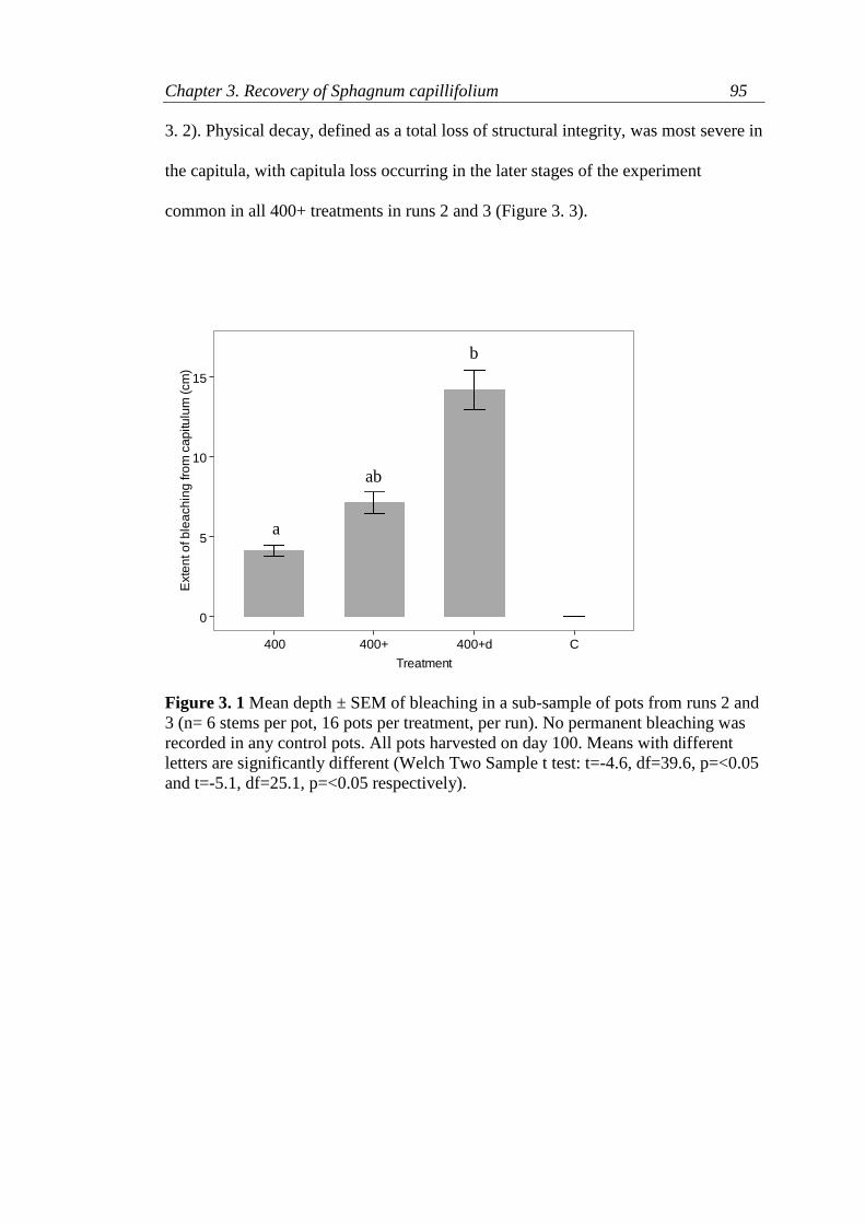
Chapter 3. Recovery of Sphagnum capillifolium 95
3. 2). Physical decay, defined as a total loss of structural integrity, was most severe in
the capitula, with capitula loss occurring in the later stages of the experiment
common in all 400+ treatments in runs 2 and 3 (Figure 3. 3).
Figure 3. 1 Mean depth ± SEM of bleaching in a sub-sample of pots from runs 2 and
3 (n= 6 stems per pot, 16 pots per treatment, per run). No permanent bleaching was
recorded in any control pots. All pots harvested on day 100. Means with different
letters are significantly different (Welch Two Sample t test: t=-4.6, df=39.6, p=<0.05
and t=-5.1, df=25.1, p=<0.05 respectively).
0
5
10
15
400 400+ 400+d C
Treatment
Exte
nt o
f b
lea
ch
ing
fro
m c
ap
itu
lum
(cm
)
a
ab
b
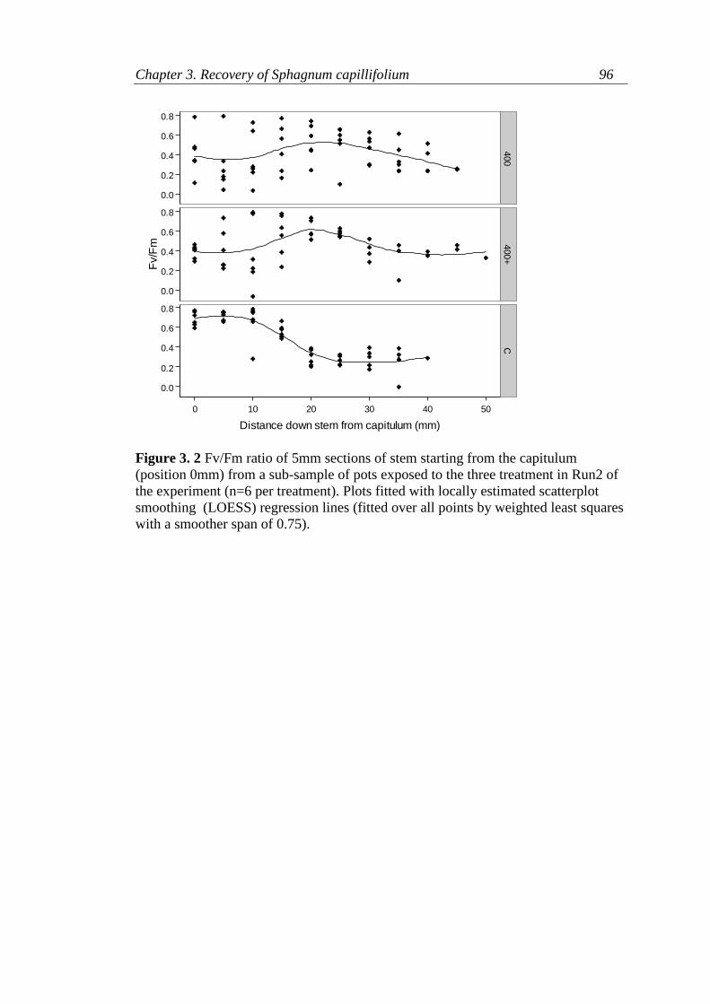
Chapter 3. Recovery of Sphagnum capillifolium 96
Figure 3. 2 Fv/Fm ratio of 5mm sections of stem starting from the capitulum
(position 0mm) from a sub-sample of pots exposed to the three treatment in Run2 of
the experiment (n=6 per treatment). Plots fitted with locally estimated scatterplot
smoothing (LOESS) regression lines (fitted over all points by weighted least squares
with a smoother span of 0.75).
0.0
0.2
0.4
0.6
0.8
0.0
0.2
0.4
0.6
0.8
0.0
0.2
0.4
0.6
0.8
400
400+
C
0 10 20 30 40 50
Distance down stem from capitulum (mm)
Fv/F
m

Chapter 3. Recovery of Sphagnum capillifolium 97
Figure 3. 3 The number of stems showing capitulum decay, defined as the distance from
the capitulum down the stem showing bleaching and/or reduced structural integrity, at each
sampling time for each treatment during runs 2 and 3 of the experiment (n=8 stems per
treatment per sampling time per run). No capitulum decay occurred in control pots.
3.5.2 Chlorophyll florescence
Throughout each run of the experiment the control pots had an Fv/Fm ratio
closest to 0.7 but with distinct low periods during Run 1 and Run 3 (Figure 3. 4). In
Runs 1 and 2 of the experiment the control stems had higher Fv/Fm ratios than stems
from pots exposed to the temperature treatments. The most appropriate linear mixed
effects model showed that both the fixed terms of Day and Treatment were
significant as well as the interaction between Day and Treatment while pot was
found to be the best random effects term to account for additional variation in the
data beyond the fixed effects (Table 3.3, Figure 3. 5).
0
5
10
15
0
5
10
15
23
1 7 19 28 40 56 88 100
Day
Nu
mb
er
of S
tem
s w
ith
Ca
pitu
lum
De
ca
y
Treatment
400
400+
400+D
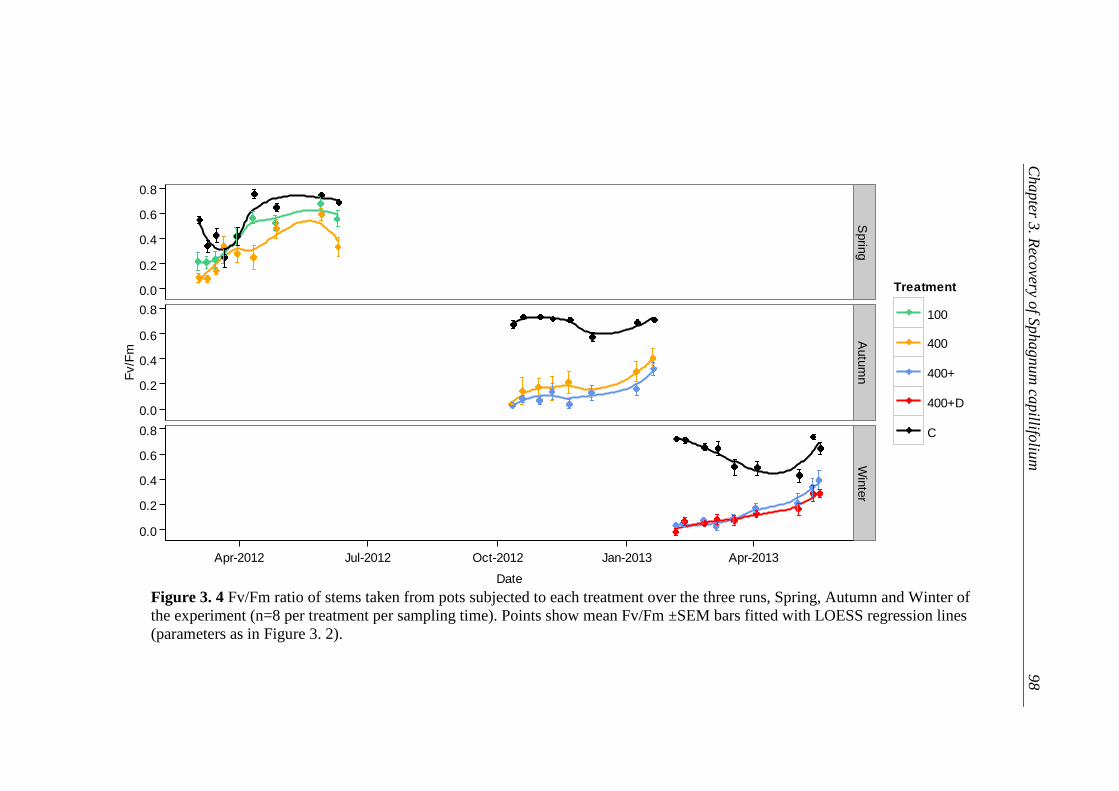
Figure 3. 4 Fv/Fm ratio of stems taken from pots subjected to each treatment over the three runs, Spring, Autumn and Winter of
the experiment (n=8 per treatment per sampling time). Points show mean Fv/Fm ±SEM bars fitted with LOESS regression lines
(parameters as in Figure 3. 2).
0.0
0.2
0.4
0.6
0.8
0.0
0.2
0.4
0.6
0.8
0.0
0.2
0.4
0.6
0.8
Sprin
gA
utu
mn
Win
ter
Apr-2012 Jul-2012 Oct-2012 Jan-2013 Apr-2013
Date
Fv/F
m
Treatment
100
400
400+
400+D
C
Chapter 3
. Reco
very of S
phagnum
capillifo
lium
98
0.0
0.2
0.4
0.6
0.8
0.0
0.2
0.4
0.6
0.8
0.0
0.2
0.4
0.6
0.8
Sprin
gA
utu
mn
Win
ter
Apr-2012 Jul-2012 Oct-2012 Jan-2013 Apr-2013
Date
Fv/F
m
Treatment
100
400
400+
400+D
C

Chapter 3. Recovery of Sphagnum capillifolium 99
Table 3.3 Results of linear mixed effects model of the Fv/Fm ratio (transformed
using Arc Sine transformation) with appropriate model selected using AIC criteria to
determine random and fixed effects and a Wald test for fixed term significance.
Models with the lowest AIC criteria and thus largest negative delta AIC (∆AIC) were
selected. MC = moisture content of Sphagnum stems at time of measurement.
Model AIC ΔAIC
Random Effects
MC+Pot+Run:Pot+Block+Run+Hum+Run:Hum
MC+Pot+Run:Pot+Block+Run+Hum
MC+Pot+Run:Pot+Block+Run
MC+Pot+Run:Pot+Block
MC+Pot+Run:Pot
MC+ Pot
MC
Fixed Effects
Treatment+Day
Treatment
Day
-220.7
-222.7
-224.7
-226.7
-225.2
-227.2
-211.5
-280.8
-275.4
-151.8
−
-2.0
-4.0
-6.0
-4.5
-6.5
+9.2
−
+5.4
+129
Wald Test of Final Model
Fixed Effect Treatment+Day Random Effect MC+ Pot
Chi Sq Df P value
Treatment
Day
226.4
26.1
4
8
<0.001
0.001026
Figure 3. 5 Amount of within treatment variance explained by the different random
effects terms in the largest mixed effect model described in Table 3.3. The final
model only included the random effect terms Pot and MC (moisture content).
0.00
0.01
0.01
0.02
0.02
0.03
0.03
Pot Run:Pot MC Hum Run:Hum Block Run Residual
Var
ian
ce
Random Effect Term

Chapter 3. Recovery of Sphagnum capillifolium 100
3.5.3 CO2 Exchange
NPP, CO2 exchange measured at a light intensity of 2000 µmol m2 s-1, varied
considerably between runs, across sampling times and treatments ranging from -
84±13 to 252±26 µmol g-1 (dry weight) day-1 with greatest NPP in control pots
during Run 2, the Autumn run (Figure 3. 6). NPP of temperature treated pots was
only noticeably lower during the first half of runs 1 and 2, with generally less
obvious treatment differences when NPP was lower. In general respiration rate,
measured when light intensity was <1 µmol m2 s-1, was less variable between
treatments than NPP (Figure 3. 7) during both runs 2 and 3 (no respiration
measurements were made during run 1 and measurements made on only three
occasions during the first half of run 2, as pots in all treatment groups became
infected with mould making gas exchange measurements on whole pots
inappropriate). Respiration rate also varied less between runs, ranging from -105±33
to -13±22 µmol g-1 (dry weight) day-1 in Run 2 and -103±11 to 17±12 µmol g-1 (dry
weight) day-1 in Run 3.
The most appropriate linear mixed effects model of NPP, respiration and
fluorescence showed that both the fixed terms of Day and Treatment were significant
(Table 3. 4). In contrast, Day was not found to be significant in models of respiration
rate (Table 3. 5) with Hummock and Block the best random effects terms to explain
the variance beyond the Treatment effect (Figure 3. 8). Common to both the models
of NPP and respiration was that the random effects described in the models explained
little of the within treatment variance.
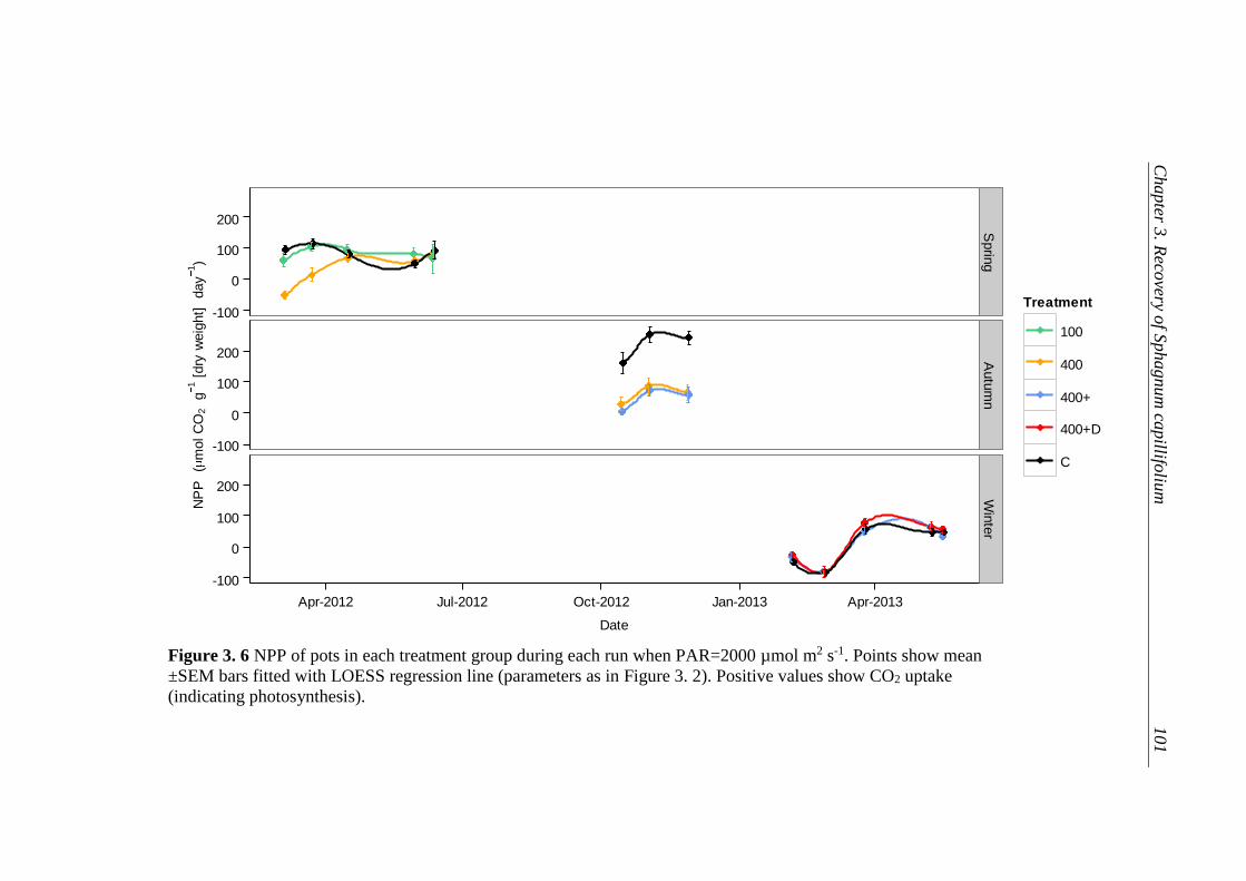
Figure 3. 6 NPP of pots in each treatment group during each run when PAR=2000 µmol m2 s-1. Points show mean
±SEM bars fitted with LOESS regression line (parameters as in Figure 3. 2). Positive values show CO2 uptake
(indicating photosynthesis).
-100
0
100
200
-100
0
100
200
-100
0
100
200
Sprin
gA
utu
mn
Win
ter
Apr-2012 Jul-2012 Oct-2012 Jan-2013 Apr-2013
Date
NP
P
(m
ol C
O2
g1 [
dry
weig
ht]
day
1)
Treatment
100
400
400+
400+D
C
Chapter 3
. Reco
very of S
phagnum
capillifo
lium
101

Figure 3. 7 Respiration of pots in each treatment group in runs 2 and 3 of the experiment measured when PAR = <1 µmol m2 s-1. Points show
mean ±SEM bars fitted with LOESS regression line (parameters as in Figure 3. 2). The lower the negative values, the higher the rate of
respiration.
Chapter 3
. Reco
very of S
phagnum
capillifo
lium
102
-100
0
100
200
-100
0
100
200
-100
0
100
200
Sprin
gA
utu
mn
Win
ter
Apr-2012 Jul-2012 Oct-2012 Jan-2013 Apr-2013
Date
NP
P
(m
ol C
O2
g1 [
dry
weig
ht]
day
1)
Treatment
100
400
400+
400+D
C
-125
-100
-75
-50
-25
0
-125
-100
-75
-50
-25
0
Autu
mn
Win
ter
Nov-2012 Dec-2012 Jan-2013 Feb-2013 Mar-2013 Apr-2013 May-2013
Date
Rate
of
Respiration (
mol C
O2
g1 [
dry
weig
ht]
day
1)
Treatment
400
400+
400+D
C

Chapter 3. Recovery of Sphagnum capillifolium 103
Table 3. 4 Results of linear mixed effects model of NPP (µmol CO2 g[dry weight]-1
day-1) with smallest model with the lowest AIC shown in bold.
Model AIC ΔAIC
Random Effects
Run+Pot+Hum+Run:Hum+Run:Pot+Block
Run+Pot+Hum+Run:Hum+Run:Pot
Run+Pot+Hum+Run:Hum
Run+Pot+Hum
Run+Pot
Run
Fixed Effects
Treatmment+Day
Treatment
Day
3409
3407
3405
3403
3404
3423
3467
3520
3486
-2
-4
-6
-5
+14
0
+53
+96
Wald Test of Final Model
Fixed Effect Treatment+Day Random Effect Pot
Chi Sq Df P value
Treatment
Day
33.13
70.73
4
4
<0.001
<0.001
Figure 3. 8 Amount of within treatment variance explained by the different random
effects terms in the largest mixed effect model described in Table 3. 4. The final
model, with the lowest AIC, only included the random effects terms Pot.
0.00E+00
5.00E+02
1.00E+03
1.50E+03
2.00E+03
2.50E+03
3.00E+03
3.50E+03
4.00E+03
Pot Run:Pot Run:Hum Hum Block Run Residual
Var
ian
ce
Random Effect Term
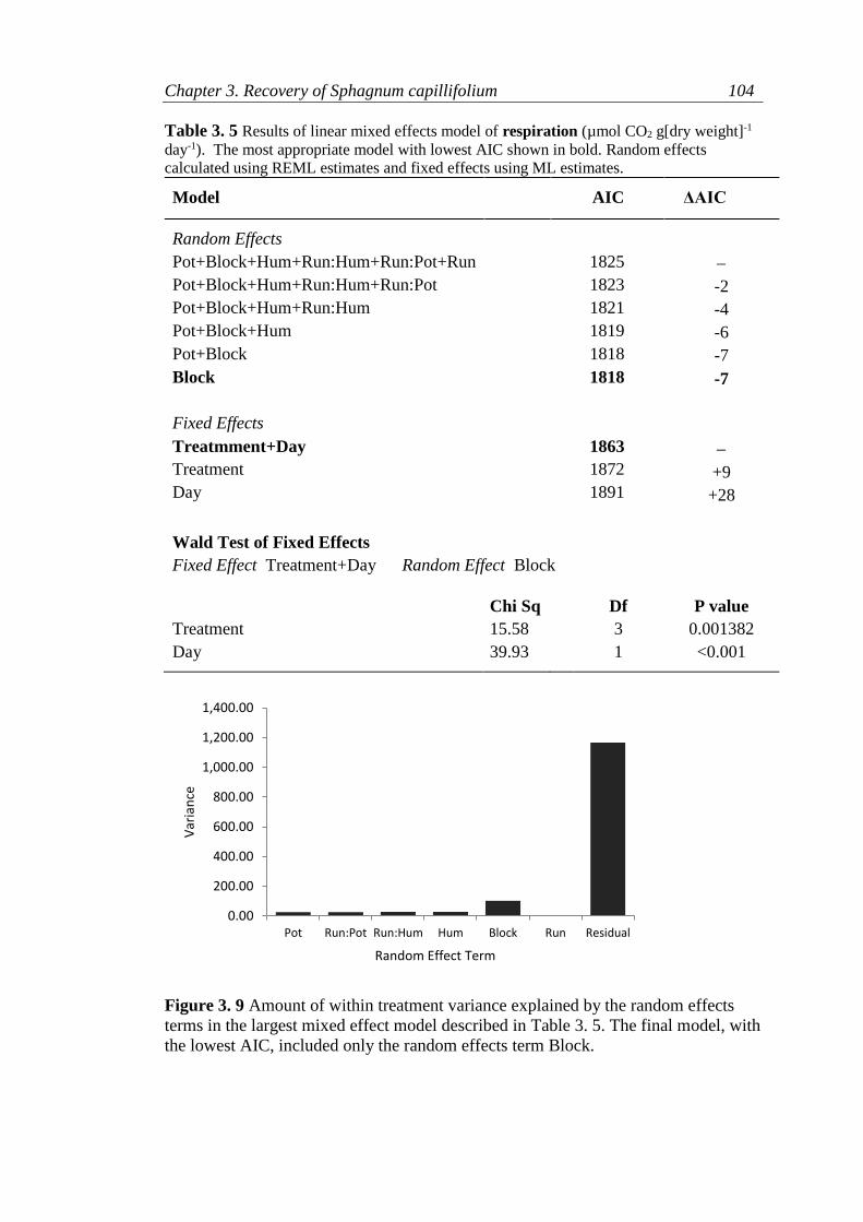
Chapter 3. Recovery of Sphagnum capillifolium 104
Table 3. 5 Results of linear mixed effects model of respiration (µmol CO2 g[dry weight]-1
day-1). The most appropriate model with lowest AIC shown in bold. Random effects
calculated using REML estimates and fixed effects using ML estimates.
Model AIC ΔAIC
Random Effects
Pot+Block+Hum+Run:Hum+Run:Pot+Run
Pot+Block+Hum+Run:Hum+Run:Pot
Pot+Block+Hum+Run:Hum
Pot+Block+Hum
Pot+Block
Block
Fixed Effects
Treatmment+Day
Treatment
Day
1825
1823
1821
1819
1818
1818
1863
1872
1891
-2
-4
-6
-7
-7
+9
+28
Wald Test of Fixed Effects
Fixed Effect Treatment+Day Random Effect Block
Chi Sq Df P value
Treatment
Day
15.58
39.93
3
1
0.001382
<0.001
Figure 3. 9 Amount of within treatment variance explained by the random effects
terms in the largest mixed effect model described in Table 3. 5. The final model, with
the lowest AIC, included only the random effects term Block.
0.00
200.00
400.00
600.00
800.00
1,000.00
1,200.00
1,400.00
Pot Run:Pot Run:Hum Hum Block Run Residual
Var
ian
ce
Random Effect Term

Chapter 3. Recovery of Sphagnum capillifolium 105
3.5.4 New Growth
New growth during the duration of the experiment arose in the form of new,
smaller and more elongated auxiliary stems and was found in all treatments after 100
days in Run 1 and Run 3 of the experiment. No new growth was found in any of the
pots harvested in Run 2 (Figure 3. 10). Two distinct zones of growth were apparent
in both Run 1 and Run 3 with new stems growing from the upper portions of stems
(here after referred so as side innovations) and stems which grew from the lowest
portion of an original stem (base innovations) (Figure 3. 11a, Appendix 3.7). In both
Run 1 and 3 most new growth occurred in pots which had been subjected to the
higher temperature treatments as opposed to control pots (Figure 3. 10). Significantly
more new growth was seen in Run 1 in both control and temperature treatment pots
than in Run 3 (Figure 3. 10).
Figure 3. 10 New growth (measured as biomass dry weight) shown as a ratio to total original
sample biomass dry weight for each treatment and run of the experiment. Points show the
mean percentage ±SEM (n=16 per treatment per run). *C shows significantly higher growth
than control treatment group in run3 (t=-2.4, df=15.9, p=0.03), *100 shows significantly
higher growth than 100 treatment group in run 1(t=-3.8332, df=22.9, p=<0.001). No new
growth was observed in any treatment group in run 2.
0.00
0.01
0.02
0.03
C 100 400 400+ 400+D
Treatment
Ra
tio o
f Ne
w B
iom
ass
to O
rig
ina
l Bio
ma
ss
Run
1
2
3
* C
* 100

Chapter 3. Recovery of Sphagnum capillifolium 106
The location (distance from capitulum) at which new side innovations grew
correlated to the depth of bleaching (Figure 3. 11) with new side innovations
growing from unbleached original stem immediately below the area of bleaching
(Appendix 3.10). A greening of the area immediately below this was often observed
in stems which did not show any auxiliary growth (Appendix 3.7).
Figure 3. 11 The location of new growth found in a subsample of 16 pots per treatment per
run showing (a) the total number of new side and base innovations seen in runs 2 and 3 and
(b) the mean location of new auxiliary side innovations in relation to the mean depth of
bleaching in the same pot shown with StE bars.
1 3
0
250
500
750
100 400 400+ 400+d c 100 400 400+ 400+d c
Treatment
Nu
mb
er
of S
tem
s
Location
Base
Side
0
5
10
15
0 5 10 15
Mean Depth of Decay (cm from capitulum)
Lo
ca
tio
n o
f n
ew
ste
m (
cm
fro
m c
ap
itu
lum
)
Treatment
400+
400+d
c
(a)
NA NA NA NA
(b)

Chapter 3. Recovery of Sphagnum capillifolium 107
3.6 Discussion
3.6.1 Photosynthetic Capacity and CO2 Exchange
The photosynthetic capacity, as indicated by chlorophyll fluorescence and
CO2 assimilation, of the upper most sections and capitula of S. capillifolium stems
was found to vary considerably between temperature treatments, throughout and
between each run of the experiment. The highest maximum quantum yield of
photosystem II (MQY), shown by the Fv/Fm ratio (Maxwell and Johnson, 2000), in
every run, and the closest to the accepted healthy plant ratio of around 0.75 (Demmig
and Björkman, 1987), was found in control pots which had not been subjected to a
temperature treatment. Pots which were subjected to the temperature treatments
showed a general increase in MQY throughout the duration of each run, with
perceivably quicker recovery to healthy Fv/Fm ratios in the less severe treatments
with lower maximum surface temperatures and residency times.
The least amount of damage, in terms of reduction in photosynthetic capacity,
was seen in pots exposed to the temperature treatment of 100oC where capitula had
an Fv/Fm ratio closest to those of the control pots throughout the duration of the
spring run of the experiment. This being the least damaging treatment is consistent
with the observation that it induced the least amount of bleaching, which suggests
that surface temperatures and residence time of this magnitude do not cause severe
damage in S.capillifolium with a pre-burn moisture content of around 90%. Pots
treated with a maximum surface temperature of 400oC showed the greatest reduction
in MQY when compared to control pots, however little difference was detected in
MQY between 400oC treatments when the maximum surface temperature residence

Chapter 3. Recovery of Sphagnum capillifolium 108
time and pre-burn moisture content was varied. This shows measure of the
maximum temperature reached at the surface of the Sphagnum layer may be a
sufficient indicator of the potential short term impact on photosynthetic capacity and
that mechanisms for damage in plant cells brought about by fire, such as protein
denaturation or lipid mobility shown in other plants (Levitt, 1972) can be brought
about by exposure to surface temperatures of around 400oC for just 3 seconds in
S.capillifolium at a pre-burn moisture content of around 90%.
Another important observation beyond the effect of high temperatures on
photosynthetic capacity was that the MQY varied both within a run over time and
between runs suggesting that short term changes in environment and seasonality are
also important. This was demonstrated by the control pots, which did not show the
steady increase in MQY over time as seen in temperature treated pots, rather
considerable variation between sample days.
An optimum stem moisture content for photosynthesis has widely been
shown in Sphagnum with declining rates of CO2 assimilation coupled with a
reduction in stem moisture content with the water needed for optimum
photosynthesis varying between species (eg. Clymo, 1973, Williams and Flanagan,
1996, Schipperges and Rydin, 1998, Adkinson and Humphreys, 2011, Silvola and
Aaltonen, 1984, Robroek et al., 2009, Titus et al., 1983, Grace, 1973, Titus and
Wagner, 1984, Strack et al., 2009) and seasonally (eg. Johansson and Linder, 1980,
Titus et al., 1983). Specifically, the MQY measured using chlorophyll fluorescence
has been shown to decline with reduced stem moisture content in Sphagnum (van

Chapter 3. Recovery of Sphagnum capillifolium 109
Gaalen et al., 2007). Although the aim of this study was to limit environmental
variation by maintaining steady moisture conditions to help show the effect of the
temperature treatments, inevitably stem moisture content did vary to some degree
within and between runs of the experiment. The effect of stem moisture content was
demonstrated here in the mixed effects model of Fv/Fm measurements in which stem
moisture content accounted for the most within treatment and sample day variation
with lowest MQY in control pots corresponding to lower stem moisture content and a
particularity warm period during Run 1. During Run 3, the winter run of the
experiment, it was also found that the lowest MQY found in control pots occurred
after a period of a few days when the Sphagnum had frozen. This suggests that the
variation in the MQY in control pots reflected environmental conditions and
furthermore that photosynthetic capacity was able to recover from the stem moisture
content and the temperature ranges experienced during the experiments.
Sphagnum has been shown to tolerate desiccation up to a critical moisture
threshold (Schouwenaars and Gosen, 2007), the point at which net photosynthesis
ceases (Schipperges and Rydin, 1998), suggesting that the drying experienced in
control pots during this study was survivable and did not drop below this threshold.
An important avenue for future experimentation would be to determine the
interaction between exposure to fire and periods of post burn desiccation as there was
some evidence for this here in the 400+D treatment. Sphagnum samples from this
treatment were dried to a moisture content of 80% prior to burning, but even when
placed in the same conditions as all other treatments and watered frequently were
consistently drier up to 88 days post burning. This could be caused by the water

Chapter 3. Recovery of Sphagnum capillifolium 110
transport and holding capacity of the Sphagnum being compromised by drying and
subsequent exposure to high temperatures suggesting that fire may make Sphagnum
more vulnerable to long term damage brought about by drought by increasing the
likelihood of drying below the critical threshold.
Post burn conditions are also important when considering the use of
chlorophyll fluorescence for quantifying recovery in the field, as these experiments
show that measurements on burnt Sphagnum have to be made concurrently with un-
burnt samples from the same site to take account of variation in MQY brought about
by environmental conditions. Confounding this is that short term changes in
environment may have long term influences on primary productivity in Sphagnum
(Backéus, 1988, McNeil and Waddington, 2003) making it necessary for
fluorescence measurements, and indeed other measures of photosynthetic capacity, to
be a long term form of monitoring rather than a “snap-shot” measurement which may
not be representative of differences in MQY brought about by burning alone.
It is important to note here that the chlorophyll fluorescence measurements in
this study were not made on the same capitula over time but on different capitula or
part of stem which made up the surface of pot, often the uppermost part of a stem if
there was capitulum loss or new auxiliary capitula, at each sampling time. These
measures of photosynthetic capacity must not therefore be interpreted as recovery in
the photosynthetic capacity of one capitulum following exposure to high
temperatures, but rather a reflection of whole pot recovery. However, it has been
shown that isolated capitula are more susceptible to damage than those within a

Chapter 3. Recovery of Sphagnum capillifolium 111
tighter cluster of other stems (Schipperges and Rydin, 1998) so single capitula
measurements may not always be representative of the whole pot. Understanding
how larger samples, better representative of a hummock, respond to burning was the
basis for whole pot measurements of CO2 exchange.
Whole pot measurements of CO2 assimilation, NPP, largely reflected the
treatment effects on MQY indicated by chlorophyll fluorescence but with the notable
exception of the lack of treatment effect on NPP in the winter (Run 3). During Run 1
and Run 2, the spring and autumn runs respectively, the control pots showed higher
NPP than the 400oC temperature treatments with some degree of recovery in the
temperature treated pots in Run 1, indicated by a return to similar NPP as the control
pots. Recovery of the temperature treated pots was not seen in either Run 3 or Run 2,
but this may be a reflection of measurements not being continued throughout the
duration if the Run 2 due to the presence of mould in the latter weeks of the run.
Unlike the 400oC treatments NPP in the 100oC treatment did not differ significantly
to the rate measured in the control pots and so again suggests that the higher
temperature treatment had a more detrimental effect on photosynthesis. This supports
the observations made of MQY that the temperatures experienced at the Sphagnum
surface during a fire may be a good indication of the degree of physiological damage
to Sphagnum. When comparing respiration between treatments there is not such a
clear treatment effect, despite it still being a significant term in the mixed effects
model. This however is likely due to the pronounced differences in respiration rates
observed on day 1 between the control pots and temperature treated pots in Run 2.
Again there was considerable variation between sampling days particularly in Run 3,
Chapter 3. Recovery of Sphagnum capillifolium 112
the winter run, when, as with NPP, there was considerable temporal variation but no
detectable difference between treatments. During both Runs 2 and 3 the NPP of
temperature treated pots followed the same temporal pattern of NPP of control pots.
This suggests that NPP in all pots was determined by other factors beyond the
temperature treatments as was also indicated from the chlorophyll fluorescence
results.
Sphagnum has been found to exhibit strong seasonal variation in production
with short day photoperiods (Gerdol, 1995) and low temperatures associated with up
to a five-fold reduction in growth (Gerdol et al., 1998). The findings here support
this seasonality shown here by the lack of CO2 assimilation during the winter run of
the experiment. However this is confounded by the lower stem moisture content
experienced throughout the winter run which as discussed previously could account
for low NPP in the control pots. However, the implications for this in the context of
prescribed burning is that if photosynthesis and growth rates are lower during the
colder and shorter photoperiod days of winter months, then rates of recovery could
be much slower following fires which have taken place early in the legal burning
season (October through to February) when compared to burns which happen at the
tail-end of the legal burning season (March/April). Seasonality is also an important
consideration when formulating monitoring systems to determine the impact of fire
on Sphagnum, as making CO2 assimilation measurements during winter alone may
not allow for the full detection of the impact burning has had on Sphagnum as
comparative unburnt Sphagnum may naturally show lower rates of photosynthetic

Chapter 3. Recovery of Sphagnum capillifolium 113
capacity and thus any differences between burnt and unburnt may be less
pronounced.
3.6.2 New Growth
New growth in the form of side and base innovations growing from original
stems were only found in Run 1 and 2 of the experiment. These runs were classed as
summer and spring runs respectively with Run 2 occurring throughout the winter
months (October to January). Sphagnum productivity has been found to be lower in
winter months (Clymo, 1970, Clymo and Hayward, 1982) with higher growth rates
correlating well with longer photoperiods in Sphagnum magellanicum and Sphagnum
papillosum (Li and Glime, 1991). Low light levels, as recorded for Run 2, the winter
run of the experiment, could therefore account for the lack of new growth observed.
An additional control on growth is night-time temperature and S.capillifolium has
been demonstrated to have a five-fold increase in growth at a night-time temperature
of 15oC compared to 5oC (Gerdol et al., 1998). The temperatures recorded during
Run 2 declined from around day 50, making them lower than those in Run 1, so these
low temperatures could also contribute to the lack of growth observed. Run 3, which
ran over a particularly cold spring, had lower growth rates in the control pots than
Run 1 which again could be due to the shorter day lengths and lower temperatures
experienced throughout the run.
Although intuitive, it is important to highlight the differences in growth rates,
in relation to biomass production, found across the experiment at different times of
year, as it shows the need to take into account post burn conditions when assessing
Chapter 3. Recovery of Sphagnum capillifolium 114
Sphagnum recovery. Management burns for instance occurring in the spring time
may show faster rates of Sphagnum recovery due to the more favourable growing
conditions after burning, while autumn burns may show much slower apparent rates
of recovery. This has implications for using Sphagnum damage, as indicated by lack
of recovery, as a post-burn indication of fire severity as time of year may be more
important for recovery than actual characteristics of the fire. In addition, other post
fire conditions, most notably the moisture status of the Sphagnum layer and height of
the water table may retard or promote growth with responses varying between
species (Robroek et al., 2007, Rochefort et al., 2002). This would make it necessary
to include post burn environmental variables and a method to assess Sphagnum over
time when formulating a system to assess damage to the Sphagnum layer post burn.
A common observation regarding new growth throughout the experiment was
the very distinct zones in which the new innovations originated. The side
innovations appeared to be very similar to those described by Clymo and Duckett
(1986), appearing bright green and originating at the base of existing branches from
an area of outer stem cortex distinctly greener than the surrounding stem. Clymo and
Duckett suspected that the ability of Sphagnum to produce new shoots in this manor
was a widespread and important mechanism to overcome random or systematic
disturbance events and has since been demonstrated in a number of species including
S.capillifolium (Clymo and Duckett, 1986, Hamilton, 2000, Rochefort et al., 2002).
The production of new innovations in response to fire has been observed in the field
(Hamilton, 2000) suggesting the side innovations observed here were not just a
product of experimental conditions. Building on these observations, here it was
Chapter 3. Recovery of Sphagnum capillifolium 115
found that the more severe temperature treatments, in terms of maximum surface
temperatures and temperature residency time, induced more production of side
innovations with the least severe temperature treatment (100 ºC for 3 seconds at the
surface) promoting a similar quantity of new innovations as the control pots in Run1.
The results suggest that this difference in recovery was likely due to the temperatures
experienced at the Sphagnum surface and associated subsequent loss of capitula.
Stems have the ability to recover from lower surface temperatures, which may not
permanently damage the capitulum, and thus plants do not need to replace capitula,
the site of greatest photosynthesis. However, when capitula are severely damaged
side innovations are induced to replace the capitula and thus restore the
photosynthetic ability at the surface. During Run1 it was evident that during the 100
day period of the experiment new capitula had reached the surface of the pots,
replacing those lost. This substantiates the observations of Hamilton (2000) who
noted some patches of Sphagnum in the field produced new green capitula on the
surface as well as other areas in which capitula regained colouration after bleaching.
The treatment which was intended to be fatal to S.capillifolium (treatment 400+D)
was still found to result in new growth suggesting it would take even higher surface
temperatures and temperature residency times to stop S.capillifolium regenerating in
this way. However, as Clymo and Duckett (1986) demonstrated discs of Sphagnum
cores taken up to 30cm below the Sphagnum surface still produced new innovations
from apparent dead material suggesting that the detrimental effects of high
temperatures would potentially have to penetrate very deep within the Sphagnum
layer to stop this type of regeneration. However, Clymo and Duckett also found that
Chapter 3. Recovery of Sphagnum capillifolium 116
light was the key stimulus for inducing the production of new innovations meaning
this could ultimately limit regeneration after fire deep within the Sphagnum layer.
The results of this experiment also showed innovations growing from the
base of stems suggest the cutting of the Sphagnum stems to achieve potted samples
of a consistent depth may have induced new growth too. It was found most new
growth in the control pots came from the area of stem closest to the cut surface with
more side stems in the most severe treatments of the two runs than bottom stems.
This suggests a potential physiological control on the site of new growth in response
to the severity and location of damage. The correlation between the maximum depth
of bleaching found within a pot and the mean depth at which new innovations grew
also suggests that damage to the capitulum triggers growth from the area
immediately below the area of stem damaged, overriding any growth from lower
sections and the production of what were observed here as base innovations.
3.7 Conclusions
The aim of this research was to determine some of the short term responses of
Sphagnum to fire by carrying out multiple measurements of recovery on
S.capillifolium, a hummock forming species common to areas of blanket in the UK,
after exposure to simulated temperatures of Calluna fires. Firstly in regards to
hypothesis [1], that the photosynthetic capacity of S. capillifolium would be reduced
following exposure to high temperatures, there was evidence that rates of, and
capacity, for photosynthesis was affected by being exposed to high surface
temperatures akin to those found in the Calluna fires. Importantly the higher 400oC
treatments caused the most pronounced reduction in photosynthesis. The 400oC

Chapter 3. Recovery of Sphagnum capillifolium 117
treatments having the most detrimental effect on Sphagnum was also mirrored in the
extent of bleaching and capitulum loss, which was minimal in the lowest 100oC
treatment. Secondly it was hypothesised that [2] a critical temperature and
temperature residence time exists above which the temperature treatments will be
lethal to S.capillifolium. Within the range of surface temperatures and temperature
residence times used here a critical threshold was not ascertained, evident by new
auxiliary stem growth found in the temperature treatment designed to be lethal,
where S.capillifolium was exposed to surface temperatures of 400oC for 30 seconds
after being dried. It must be stressed that these experiments only concerned one
species studied over three month periods within comparatively narrow maximum
burn temperature and stem moisture content ranges so cannot be used to entirely
reject the potential lethality of fire on other Sphagnum species beyond these
conditions. Instead these results give evidence that S.capillifolium has the ability to
recover from fire in certain circumstances. Beyond this there is strong evidence here
that the rate of recovery of S.capillifolium is in response to maximum temperatures
experienced at the surface as well as environmental conditions with the least amount
of re-growth during the winter months. This is an important observation to consider
when formulating assessments using Sphagnum re-growth as an indicator of the
ecological severity of a fire.

Chapter 3. Recovery of Sphagnum capillifolium 118
3.8 References
ADKINSON, A. C. & HUMPHREYS, E. R. 2011. The response of carbon dioxide
exchange to manipulations of Sphagnum water content in an ombrotrophic
bog. Ecohydrology, 4, 733-743.
ASHTON, C., REIN, G., RIVERA, J. D., TORERO, J. L., LEGG, C., DAVIES, M.
& GRAY, A. 2007. Experiments and observations of peat smouldering fires.
International Meeting of Fire Effects on Soil Properties. Barcelona:
University of Edinburgh.
BACKÉUS, I. 1988. Weather variables as predictors of Sphagnum growth on a bog.
Ecography, 11, 146-150.
BARKMAN, J. J. 1992. Plant communities and synecology of bogs and heath pools
in the Netherlands. In: VERHOEVEN, J. A. (ed.) Fens and Bogs in the
Netherlands. Dordrecht: Kluwer Academic Publishers.
BATES, D., MAECHLER, M. & BOLKER, B. 2013. lme4: Linear mixed-effects
models using S4 classes. R package version 0.999999-2. http://CRAN.R-
project.org/package=lme4.
BATES, J. W., WIBBELMANN, M. H. & PROCTOR, M. C. F. 2009. Salinity
responses of halophytic and non-halophytic bryophytes determined by
chlorophyll fluorometry. Journal of Bryology, 31, 11-19.
BENSCOTER, B. W., THOMPSON, D. K., WADDINGTON, J. M., FLANNIGAN,
M. D., WOTTON, B. M., DE GROOT, W. J. & TURETSKY, M. R. 2011.
Interactive effects of vegetation, soil moisture and bulk density on depth of
burning of thick organic soils. International Journal of Wildland Fire, 20,
418-429.
BØRSHEIM, K. Y., CHRISTENSEN, B. E. & PAINTER, T. J. 2001. Preservation of
fish by embedment in Sphagnum moss, peat or holocellulose: experimental
proof of the oxopolysaccharidic nature of the preservative substance and of
its antimicrobial and tanning action. Innovative Food Science & Emerging
Technologies, 2, 63-74.
BURCH, J. 2009. The regeneration of bryophytes after the burning of dry heat and
wet heath moorland on the North York Moors. Natural England
Commissioned Report NECR011. Sheffield: Natural England.
CARFRAE, J. A. 2005. The influence of reactive nitrogen on the ecophysiology of
ombrotrophic Sphagnum and Calluna. Ph.D., University of Dundee.
CLYMO, R. S. 1970. Growth of Sphagnum - Methods of Measurement. Journal of
Ecology, 58, 13-&.

Chapter 3. Recovery of Sphagnum capillifolium 119
CLYMO, R. S. 1973. Growth of Sphagnum - Some Effects of Environment. Journal
of Ecology, 61, 849-869.
CLYMO, R. S. & DUCKETT, J. G. 1986. Regeneration of Sphagnum. New
Phytologist, 102, 589-614.
CLYMO, R. S. & HAYWARD, P. M. 1982. The Ecology of Sphagnum In: SMITH,
A. J. E. (ed.) Bryophyte Ecology. New York: Chapman and Hall Ltd.
DAVIES, G. M. 2005. Fire behaviour and impact on heather moorland. Ph.D,
University of Edinburgh.
DAVIES, G. M., GRAY, A., REIN, G. & LEGG, C. J. 2013. Peat consumption and
carbon loss due to smouldering wildfire in a temperate peatland. Forest
Ecology and Management, 308, 169-177.
DEMMIG, B. & BJÖRKMAN, O. 1987. Comparison of the effect of excessive light
on chlorophyll fluorescence (77K) and photon yield of
O<sub>2</sub> evolution in leaves of higher plants. Planta, 171,
171-184.
DEPARTMENT FOR ENVIRONMENT FOOD AND RURAL AFFAIRS. 2007.
The Heather and Grass Burning Code [Online]. London: Department for
Environment, Food and Rural Affairs. Available:
http://www.naturalengland.org.uk/Images/heathergrassburningcode_tcm6-
7795.pdf.
FRANDSEN, W. H. 1997. Ignition probability of organic soils. Canadian Journal of
Forest Research, 27, 1471-1477.
GERDOL, R. 1995. The Growth Dynamics of Sphagnum Based on Field
Measurements in a Temperate Bog and on Laboratory Cultures. Journal of
Ecology, 83, 431-437.
GERDOL, R., BONORA, A., MARCHESINI, R., GUALANDRI, R. &
PANCALDI, S. 1998. Growth Response of Sphagnum capillifolium to
Nighttime Temperature and Nutrient Level: Mechanisms and Implications for
Global Change. Arctic and Alpine Research, 30, 388-395.
GLIME, J. M. 2007. Physiological Ecology. Bryophyte Ecology. Ebook sponsored
by Michigan Technological University and the International Association of
Bryologists.
GRACE, J. 1973. The Growth-physiology of Moorland Plants in Relation to Their
Aerial Environment, Sheffield, University of Sheffield.
GREEN, T. G. A., SCHROETER, B., KAPPEN, L., SEPPELT, R. D. & MASEYK,
K. 1998. An assessment of the relationship between chlorophyll a
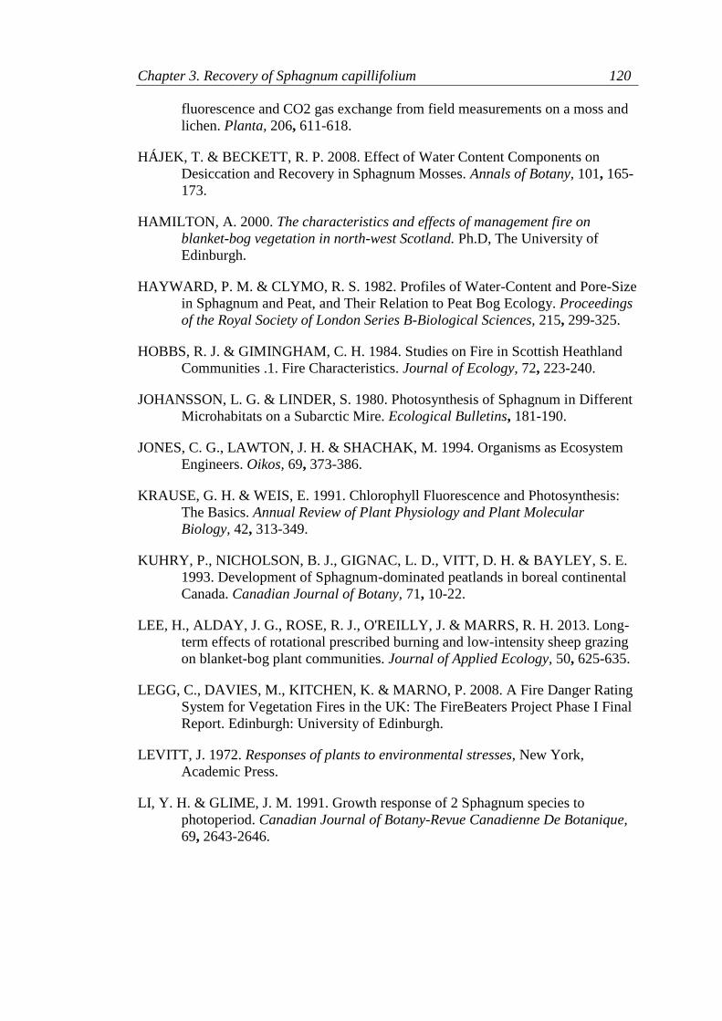
Chapter 3. Recovery of Sphagnum capillifolium 120
fluorescence and CO2 gas exchange from field measurements on a moss and
lichen. Planta, 206, 611-618.
HÁJEK, T. & BECKETT, R. P. 2008. Effect of Water Content Components on
Desiccation and Recovery in Sphagnum Mosses. Annals of Botany, 101, 165-
173.
HAMILTON, A. 2000. The characteristics and effects of management fire on
blanket-bog vegetation in north-west Scotland. Ph.D, The University of
Edinburgh.
HAYWARD, P. M. & CLYMO, R. S. 1982. Profiles of Water-Content and Pore-Size
in Sphagnum and Peat, and Their Relation to Peat Bog Ecology. Proceedings
of the Royal Society of London Series B-Biological Sciences, 215, 299-325.
HOBBS, R. J. & GIMINGHAM, C. H. 1984. Studies on Fire in Scottish Heathland
Communities .1. Fire Characteristics. Journal of Ecology, 72, 223-240.
JOHANSSON, L. G. & LINDER, S. 1980. Photosynthesis of Sphagnum in Different
Microhabitats on a Subarctic Mire. Ecological Bulletins, 181-190.
JONES, C. G., LAWTON, J. H. & SHACHAK, M. 1994. Organisms as Ecosystem
Engineers. Oikos, 69, 373-386.
KRAUSE, G. H. & WEIS, E. 1991. Chlorophyll Fluorescence and Photosynthesis:
The Basics. Annual Review of Plant Physiology and Plant Molecular
Biology, 42, 313-349.
KUHRY, P., NICHOLSON, B. J., GIGNAC, L. D., VITT, D. H. & BAYLEY, S. E.
1993. Development of Sphagnum-dominated peatlands in boreal continental
Canada. Canadian Journal of Botany, 71, 10-22.
LEE, H., ALDAY, J. G., ROSE, R. J., O'REILLY, J. & MARRS, R. H. 2013. Long-
term effects of rotational prescribed burning and low-intensity sheep grazing
on blanket-bog plant communities. Journal of Applied Ecology, 50, 625-635.
LEGG, C., DAVIES, M., KITCHEN, K. & MARNO, P. 2008. A Fire Danger Rating
System for Vegetation Fires in the UK: The FireBeaters Project Phase I Final
Report. Edinburgh: University of Edinburgh.
LEVITT, J. 1972. Responses of plants to environmental stresses, New York,
Academic Press.
LI, Y. H. & GLIME, J. M. 1991. Growth response of 2 Sphagnum species to
photoperiod. Canadian Journal of Botany-Revue Canadienne De Botanique,
69, 2643-2646.

Chapter 3. Recovery of Sphagnum capillifolium 121
LLOYD, P. S. 1968. The Ecological Significance of Fire in Limestone Grassland
Communities of the Derbyshire Dales. Journal of Ecology, 56, 811-826.
MALMER, N. & WALLÉN, B. 2004. Input rates, decay losses and accumulation
rates of carbon in bogs during the last millennium: internal processes and
environmental changes. The Holocene, 14, 111-117.
MANNINEN, S., WOODS, C., LEITH, I. D. & SHEPPARD, L. J. 2011.
Physiological and morphological effects of long-term ammonium or nitrate
deposition on the green and red (shade and open grown) Sphagnum
capillifolium. Environmental and Experimental Botany, 72, 140-148.
MAXWELL, K. & JOHNSON, G. N. 2000. Chlorophyll fluorescence: a practical
guide. Journal of Experimental Botany, 51, 659-668.
MCNEIL, P. & WADDINGTON, J. M. 2003. Moisture Controls on Sphagnum
Growth and CO2 Exchange on a Cutover Bog. Journal of Applied Ecology,
40, 354-367.
PROCTOR, M. C. F. 2003. Experiments on the effect of different intensities of
desiccation on bryophyte survival, using chlorophyll fluorescence as an index
of recovery. Journal of Bryology, 25, 201-210.
R CORE TEAM. 2013. R: A language and environment for statistical computing
[Online]. Vienna, Austria. Available: http://www.R-project.org/ [Accessed
20/5/2013 2013].
REIN, G., GARCIA, J., SIMEONI, A., TIGHAY, V. & FERRAT, L. 2008.
Smouldering natural fires: comparison of burning dynamics in boreal peat
and Mediterranean humus. WIT Transaction on Ecology and the Environment
119, 183-192.
ROBROEK, B. J. M., LIMPENS, J., BREEUWER, A. & SCHOUTEN, M. G. C.
2007. Effects of Water Level and Temperature on Performance of Four
Sphagnum Mosses. Plant Ecology, 190, 97-107.
ROBROEK, B. J. M., SCHOUTEN, M. G. C., LIMPENS, J., BERENDSE, F. &
POORTER, H. 2009. Interactive effects of water table and precipitation on
net CO2 assimilation of three co-occurring Sphagnum mosses differing in
distribution above the water table. Global Change Biology, 15, 680-691.
ROCHEFORT, L., CAMPEAU, S. & BUGNON, J.-L. 2002. Does prolonged
flooding prevent or enhance regeneration and growth of Sphagnum? Aquatic
Botany, 74, 327-341.
RODWELL, J. S. 1991. British Plant Communities. II. Mires and Heaths.
Cambridge, UK: Cambridge University Press.

Chapter 3. Recovery of Sphagnum capillifolium 122
RYDIN, H. & JEGLUM, J. K. 2006. The biology of peatlands, New York, Oxford
University Press.
SCHIPPERGES, B. & RYDIN, H. 1998. Response of photosynthesis of Sphagnum
species from contrasting microhabitats to tissue water content and repeated
desiccation. New Phytologist, 140, 677-684.
SCHOUWENAARS, J. M. & GOSEN, A. M. 2007. The sensitivity of Sphagnum to
surface layer conditions in a re-wetted bog: a simulation study of water stress
Mires and Peat, 2, 1-19.
SCOTTISH EXECUTIVE 2011. The Muirburn Code. Edinburgh: Scottish
Government.
SHEPPARD, L. J., LEITH, I. D., LEESON, S. R., VAN DIJK, N., FIELD, C. &
LEVY, P. 2012. Fate of N in a peatland, Whim bog: N immobilisation in the
vegetation and peat, leakage into pore water and losses as N2O depend on the
form of N. Biogeosciences Discuss., 9, 8141-8171.
SILVOLA, J. & AALTONEN, H. 1984. WATER-CONTENT AND
PHOTOSYNTHESIS IN THE PEAT MOSSES SPHAGNUM-FUSCUM
AND SPHAGNUM-ANGUSTIFOLIUM. Annales Botanici Fennici, 21, 1-6.
STRACK, M., WADDINGTON, J. M., LUCCHESE, M. C. & CAGAMPAN, J. P.
2009. Moisture controls on CO2 exchange in a Sphagnum-dominated
peatland: results from an extreme drought field experiment. Ecohydrology, 2,
454-461.
TITUS, J. E. & WAGNER, D. J. 1984. Carbon Balance for Two Sphagnum Mosses:
Water Balance Resolves a Physiological Paradox. Ecology, 65, 1765-1774.
TITUS, J. E., WAGNER, D. J. & STEPHENS, M. D. 1983. Contrasting Water
Relations of Photosynthesis for Two Sphagnum Mosses. Ecology, 64, 1109-
1115.
VAN GAALEN, K. E., FLANAGAN, L. B. & PEDDLE, D. R. 2007.
Photosynthesis, chlorophyll fluorescence and spectral reflectance in
Sphagnum moss at varying water contents. Oecologia, 153, 19-28.
WARD, S. E., BARDGETT, R. D., MCNAMARA, N. P., ADAMSON, J. K. &
OSTLE, N. J. 2007. Long-term consequences of grazing and burning on
northern peatland carbon dynamics. Ecosystems, 10, 1069-1083.
WILLIAMS, T. G. & FLANAGAN, L. B. 1996. Effect of changes in water content
on photosynthesis, transpiration and discrimination against 13CO2 and
C18O16O in Pleurozium and Sphagnum. Oecologia, 108, 38-46.
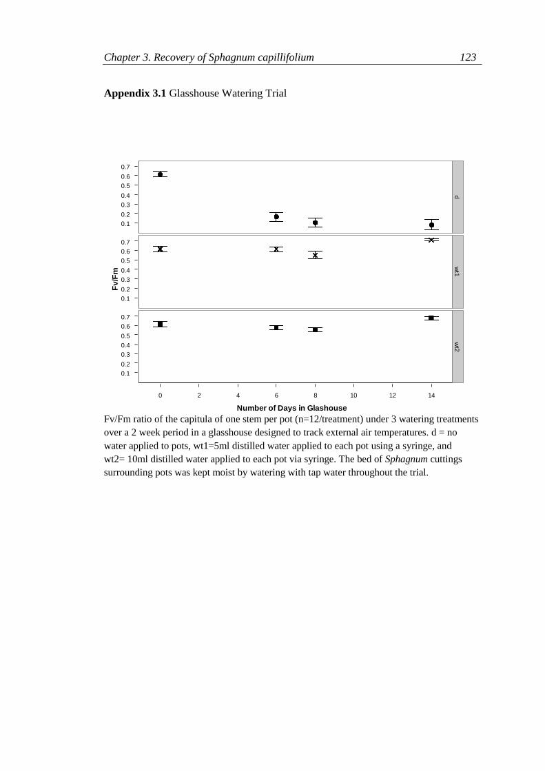
Chapter 3. Recovery of Sphagnum capillifolium 123
Appendix 3.1 Glasshouse Watering Trial
Fv/Fm ratio of the capitula of one stem per pot (n=12/treatment) under 3 watering treatments
over a 2 week period in a glasshouse designed to track external air temperatures. d = no
water applied to pots, wt1=5ml distilled water applied to each pot using a syringe, and
wt2= 10ml distilled water applied to each pot via syringe. The bed of Sphagnum cuttings
surrounding pots was kept moist by watering with tap water throughout the trial.
Number of Days in Glashouse
Fv
/Fm
0.1
0.2
0.3
0.4
0.5
0.6
0.7
0.1
0.2
0.3
0.4
0.5
0.6
0.7
0.1
0.2
0.3
0.4
0.5
0.6
0.7
0 2 4 6 8 10 12 14
dw
t1w
t2

Chapter 3. Recovery of Sphagnum capillifolium 124
Appendix 3.2 Schematic of experimental design and sampling procedure
Sphagnum
from 4
hummocks
Hummock 1 Hummock 2 Hummock 3 Hummock 4
Hummocks
make up 96
pots
96 Pots
Pots assigned
to one of three
treatments
32 Pots
Control
32 Pots
Heat Treatment 1
32 Pots
Heat Treatment 2
Pots assigned
to blocks
within tray
24 Pots
Block 1
24 Pots
Block 2
24 Pots
Block 3
24 Pots
Block 4
Pots assigned
to one of four
measuring
protocols per
block
6 Pots
Moisture Content
Analysis of
1 stem/pot
(destructive)
6 Pots
Chlorophyll
Fluorescence of
1 capitula/pot
(destructive)
6 Pots
Growth
(whole pot,
harvested at end
of each run)
6 Pots
Gas Exchange
(whole pot)
Harvesting of
pots assigned
to non-
destructive
measuring
protocol
6 Pots
New Growth
(all new stems counted)
6 Pots
New Growth
(all new stems counted and new stem
lengths measured)

Chapter 3. Recovery of Sphagnum capillifolium 125
Appendix 3.3 Maximum temperatures and temperature residency time of each
treatment
Time (s) surface temperatures achieved for each treatment used in the experiment.
Points represent the mean time the surface was above each temperature ± StE bars
(Treatment 100 n=32, Treatment 400 n=64, Treatment 400+ n=62, Treatment 400+D
n=32).

Chapter 3. Recovery of Sphagnum capillifolium 126
0
1
2
3
4
5
0 20
0
40
0
60
0
Dis
tnac
e f
rom
su
rfac
e (
cm)
Temperature (oC)
100
0
1
2
3
4
5
0 20
0
40
0
60
0
Dis
tnac
e f
rom
su
rfac
e (
cm)
Temperature (oC)
400
0
1
2
3
4
5
0 20
0
40
0
60
0
Dis
tnac
e f
rom
su
rfac
e (
cm)
Temperature (oC)
400+
0
1
2
3
4
5
0 20
0
40
0
60
0
Dis
tnac
e f
rom
su
rfac
e (
cm)
Temperature (oC)
400+D
Surface temperatures and temperatures reached at 2cm and 5cm below the surface in
samples of Sphagnum capillifolium exposed to the four different treatments. Solid
line shows maximum temperature reached at the three locations, dotted line
represents the potentially physiologically damaging temperature (45oC).
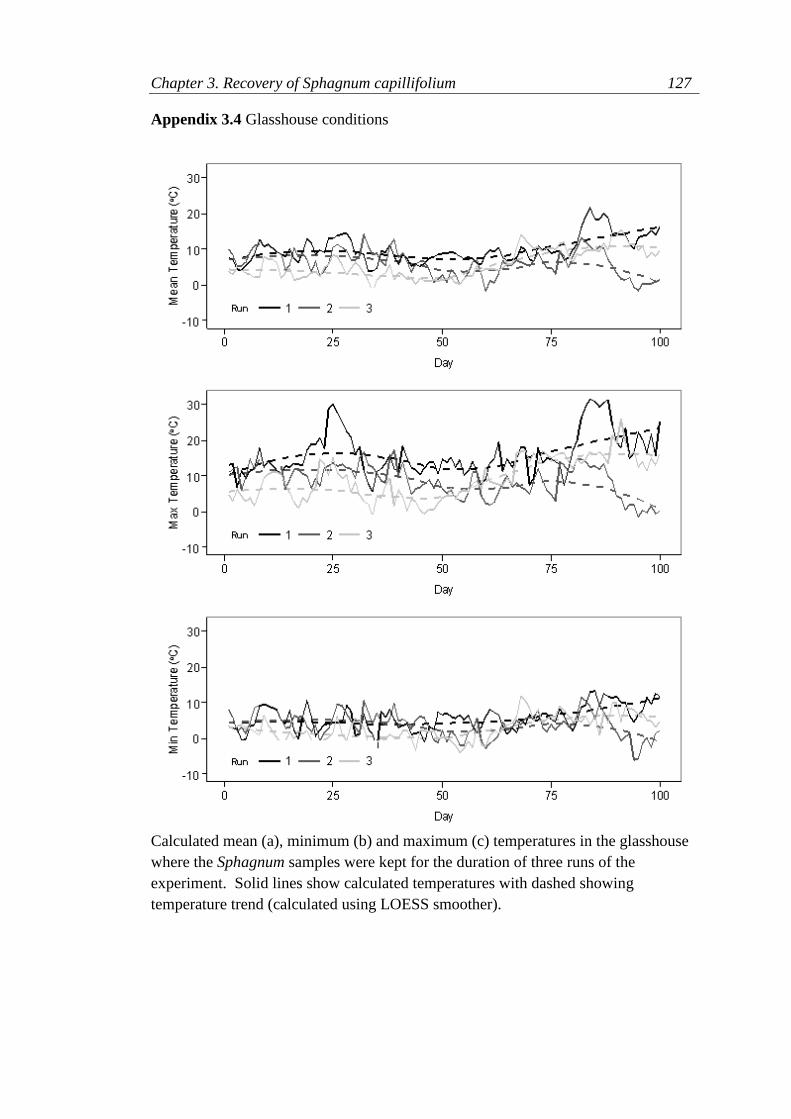
Chapter 3. Recovery of Sphagnum capillifolium 127
Appendix 3.4 Glasshouse conditions
Calculated mean (a), minimum (b) and maximum (c) temperatures in the glasshouse
where the Sphagnum samples were kept for the duration of three runs of the
experiment. Solid lines show calculated temperatures with dashed showing
temperature trend (calculated using LOESS smoother).
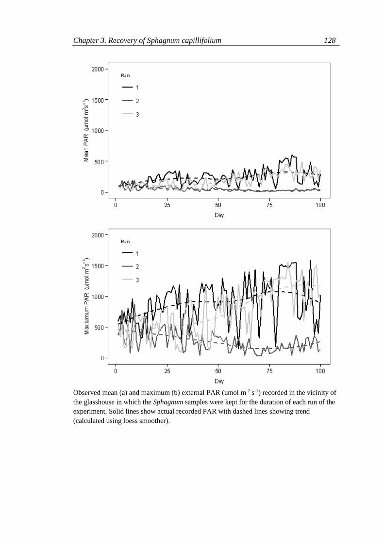
Chapter 3. Recovery of Sphagnum capillifolium 128
Observed mean (a) and maximum (b) external PAR (umol m-2 s-1) recorded in the vicinity of
the glasshouse in which the Sphagnum samples were kept for the duration of each run of the
experiment. Solid lines show actual recorded PAR with dashed lines showing trend
(calculated using loess smoother).

Chapter 3. Recovery of Sphagnum capillifolium 129
Moisture content (on a wet weight basis) of Sphagnum sampled from pots of each treatment
during each run where n=8 per treatment per sampling time.
Mean moisture contents for each treatment are shown below:
70
80
90
70
80
90
70
80
90
12
3
1 7 13 19 28 40 56 88 100
Day
Mo
istu
re C
on
ten
t (%
on
a d
ry w
eig
ht b
asis
)
Treatment
100
400
400+
400+D
C
Run Treatment
Mean Moisture
Content
(% wet weight
basis)
Mean Moisture
Content
(fresh /dry
weight)
1 Control 88.6 9.9
100 89.3 9.6
400 88.9 9.3
2 Control 92.1 10.9
400 91.2 12.6
400+ 91.5 12.5
3 Control 88.9 6.9
400+ 88.5 8.2
400+D* 79.1 6.1

Chapter 3. Recovery of Sphagnum capillifolium 130
Appendix 3.5 Rates of Photosynthesis in Sphagnum capillifolium at different light
intensities using Licor Li-6400 and specifically designed sample chamber
Rates of photosynthesis measured in seven samples of Sphagnum capillifolium at
different light intensities. Measurements were made using the light curve logging
function on the Licor Li-6400 and set to maintain sample chamber temperature at
20oC with an initial CO2 concentration of 400μmol.
Rates of photosynthesis never stabilised or declined with an increase in PAR. It was
hypothesised that this was due to the large samples of Sphagnum used within the
sample chamber, as the samples would become light saturated at different depths in
relation to light intensity. Thus damage or saturation at the surface of the sample
could be masked by the photosynthetic activity of lower sections of the sample.
-4
-2
0
2
4
6
8
10
12
0 500 1000 1500 2000 2500
Net
Pri
mar
y P
rod
uct
ivit
y (µ
mo
l CO
2g-1
[dry
w
eig
ht]
s-1
)
Light Intensity (µmol m2 s-1)
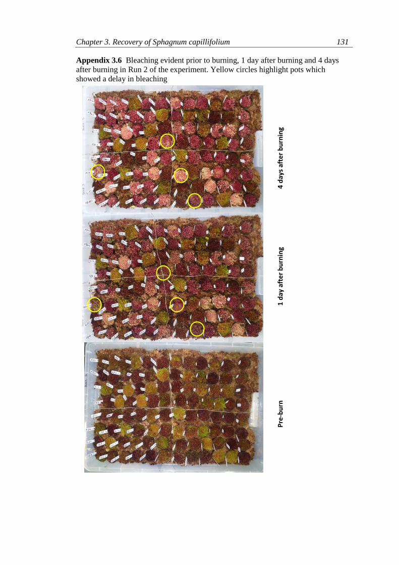
Chapter 3. Recovery of Sphagnum capillifolium 131
Appendix 3.6 Bleaching evident prior to burning, 1 day after burning and 4 days
after burning in Run 2 of the experiment. Yellow circles highlight pots which
showed a delay in bleaching
Pre
-bu
rn
4 d
ays
afte
r b
urn
ing
1 d
ay a
fte
r b
urn
ing

Chapter 3. Recovery of Sphagnum capillifolium 132
Appendix 3.7. Photographs of new auxiliary stem growth observed 100 days after
burning in runs 1 and 2 of the experiment
New side innovation growing
from original stem with
capitulum decay and eventual
loss.
New side innovation growing
from original stem showing
bleaching.
Difference in morphology of
new side innovations (top of
image) and base innovations
which grew from the bottom
cut surface of the stem (bottom
of image).

Chapter 3. Recovery of Sphagnum capillifolium 133
Post-burn
Day 4
A pot from the 400oC
treatment (Run1) 100 days
after burning showing new
capitula (green). The capitula
of most of the original stems
were heavily bleached with
widespread capitulum loss
observed throughout the pot.
An example of stems
(subjected to the 400+
treatment in Run 3) showing
the characteristic bleaching of
the capitulum and the apparent
greening of the area of stem
immediately below.
Examples of base innovations
found growing from the bottom
of original stems.
Chapter 4. Methanotrophy in Sphagnum 134
4. Methanotrophy in Sphagnum and the potential impact of fire
4.1 Abstract
Methanotrophic bacteria can be found living in symbiosis with Sphagnum
mosses in peatlands across the world (Kip et al., 2010). Their role in intercepting and
oxidising CH4 naturally produced by peatlands is increasingly being emphasised
within the context of the global atmospheric greenhouse gas budget (Chen and
Murrell, 2010). Fire, which occurs both naturally and anthropogenically on
peatlands, could potentially reduce or change the methanotrophic community and
have consequences for net CH4 emissions from peatlands. CH4 oxidation has been
reported in a large number of Sphagnum species from different microhabitats, with
rates of CH4 oxidation of up to 80 µmol CH4 g-1dw (dry weight) day-1 (Kip et al.,
2010). However, there are potential problems with the methodology used, and as yet
there is no research looking at the specific effect of fire on methanotrophy. Here we
show that experimental errors can account for oxidation rates seen in samples using
the standard methodology; we found that empty flasks produced statistically similar
CH4 fluxes to those of Sphagnum-filled flasks. Sphagnum papillosum was the only
species studied that showed detectable methanotrophy but no differences were found
between burnt and unburnt samples. These results emphasize the need for well
considered controls when estimating potential CH4 oxidation in Sphagnum using this
methodology. The results also reiterate that rates of CH4 oxidation may vary
considerably within Sphagnum and that a better understanding of the controls on CH4
oxidation in the Sphagnum layer is needed if the role of methanotrophic bacteria can
be incorporated into carbon budget models of Sphagnum-dominated peatlands.
Chapter 4. Methanotrophy in Sphagnum 135
4.2 Introduction
Peatlands store up to one third of terrestrial carbon (Gorham, 1991) making
them a significant component of the terrestrial carbon cycle. Carbon can however be
lost directly to the atmosphere from peatlands in the form of carbon dioxide (CO2)
and methane (CH4), both important greenhouse gases. CH4 has a global warming
potential (GWP) 34 times that of CO2 over a 100 year time horizon (IPCC, 2013) and
is estimated to account for 18% of global warming (Butler, 2012). Understanding the
controls on CH4 efflux to the atmosphere is therefore important if peatlands are to be
maintained and managed in ways to best maximise their carbon storage potential and
their role in mitigating climate change. Methanotrophic bacteria, predominantly
found in the aerobic zone of peat and in the Sphagnum layer, are responsible for
oxidising significant amounts of CH4 as it is transported through peat soils to the
atmosphere (Whalen, 2005), converting CH4 to CO2 and thereby reducing the GWP
of the gas emissions. This makes the balance between the production of CH4 and the
oxidation of CH4 by methanotrophic bacteria a significant component of the peatland
carbon cycle and is increasingly recognised as integral to the global atmospheric
greenhouse gas budget (Chen and Murrell, 2010, Singh et al., 2010, Chowdhury and
Dick, 2013).
Methanotrophic bacteria use CH4, produced from the breakdown of organic
material under anoxic conditions, as their sole source of carbon and energy through a
process which is oxygen-dependent, confining them mainly to the upper aerobic
layers in wetlands (Hanson and Hanson, 1996), although anaerobic CH4 oxidation
may also be widespread (Gupta et al., 2013). Methanotrophic bacteria, which are

Chapter 4. Methanotrophy in Sphagnum 136
classified as Type I or Type II, based on their physiology and phylogeny (Hanson
and Hanson, 1996), can live in mutualistic symbiosis with Sphagnum (eg. Larmola et
al., 2010, Kip et al., 2010, Parmentier et al., 2011, Stępniewska et al., 2013), living
in hyaline cells and on leaf surfaces (Raghoebarsing et al., 2005, Kip et al., 2010).
The CO2 they release provides an important source of carbon for Sphagnum
photosynthesis (Raghoebarsing et al., 2005, Parmentier et al., 2011) and is estimated
to make up to 10 to 30 % of total carbon assimilated by Sphagnum (Raghoebarsing et
al., 2005, Larmola et al., 2010). The critical role of methanotrophic bacteria
associated with the aerobic peat and Sphagnum layer in balancing CH4 production
with oxidation means that Sphagnum-dominated peatlands often have lower CH4
emissions than other wetland types (Nykänen et al., 1998) with methanotrophs
having been found to oxidise up to 100% of CH4 (Whalen, 2005). Reducing the
number, or changing the community structure, of methanotrophs in the Sphagnum
layer could therefore have a significant impact on the carbon balance of a peatland.
A potential mechanism to reduce the number of methanotrophs and thus rates
of CH4 oxidation could be fire. Fires occur both naturally on peatlands and due to
anthropogenic causes, including the routine intentional burning to clear and manage
land and for agricultural. The understanding of the interaction between fire and the
Sphagnum layer is limited but studies have shown that Sphagnum may experience
potentially biologically lethal temperatures (Davies, 2005, Glime, 2007) as well as be
consumed by a fire (Hamilton 2000). The direct consumption and heating of the
Sphagnum layer could be lethal to methanotrophic bacteria residing there and so
potentially reduce the amount of CH4 intercepted and oxidised. There is limited

Chapter 4. Methanotrophy in Sphagnum 137
research into the effect of fire on the bacterial community of peatlands and peat soils,
particularly in relation to the impact on methanogenic and methanotrophic bacteria
(Andersen et al., 2013) but a general reduction in methanotroph population size
together with an increase in the dominance of type II methanotrophs has been
demonstrated on a burned Calluna vulgaris-(L.) Hull dominated peatland (Chen et
al., 2008) this suggests that fire has the ability to alter the methanotrophic
community so the potential to change rates of CH4 oxidization.
4.3 Aims
The aim of this research was to investigate the magnitude of CH4 oxidation
by methanotrophic bacteria associated with three Sphagnum species common in UK
blanket bog, and to examine the potential influence of fire, via its effect on the
methanotrophic populations. A lab-based experiment was used to enable CH4
oxidation rates in samples of Sphagnum to be determined in non-CH4-limiting
conditions following the methodology set out in Larmola et al. (2010). The potential
impact of fire on methaotrophic activity in the Sphagnum layer was investigated by
subjecting samples to a temperature treatment designed to simulate a temperatures of
a heath fire. It was hypothesized that: [1] CH4 oxidation would differ between
species collected from different microhabitats using the experimental technique and
that [2] Sphagnum samples subjected to a temperature treatment would show lower
CH4 oxidation rates, because temperatures experienced during the fire treatment
would be lethal to methanotrophs.

Chapter 4. Methanotrophy in Sphagnum 138
4.4 Methodology
4.4.1 Sampling Site
Sphagnum capillifolium (Ehrh.) Hedw., Sphagnum papillosum Lindb. and
Sphagnum fallax H. Klinggr. were collected from Whim Moss, an ombrotrophic
CH4 producing blanket bog at an altitude of 282m situated near Penicuik, South East
Scotland (NT203532) (Sheppard et al., 2014). A National Vegetation Classification
(NVC) M19, Calluna vulgaris/Eriophorum vaginatum blanket mire (Rodwell 1991),
Whim Moss has a mean air temperature (2003–2009) of 8.6oC (ranging from −9.2 to
27.7 oC) (Sheppard et al., 2012).
4.4.2 Experimental Methodology
Based on the methodology set out in Larmola et al. (2010) samples of
Sphagnum were allocated randomly to a 1000ml glass jar (Kilner®) and sealed with a
metal vacuum lid and metal screw band (Kilner®) in which a 3-way valve (Discofix®
3-way Stopcock) with 4cm section of Bev-a-Line® tubing on the underside had been
sealed into a gas tight hole (Figure 4. 1). Prior to each run of the experiment jars
were washed and sterilised using 1% Nuetracon® (Decon Laboratories Ltd) solution
and dried at 70oC for 24 hours. Once filled with Sphagnum and sealed, 10 ml of
headspace air was removed from each jar using a syringe attached to the valve before
being injected with 10 ml of pure CH4 to give a starting CH4 concentration just above
10,000 ppm, exact concentration being dependent on volume of Sphagnum and thus
headspace volume in the jar. Once spiked with CH4 each jar was shaken by hand for
10 seconds to help the mixing of CH4 and headspace air. Once shaken, a 4 ml sample
was removed with a syringe via the valve. Each sample was withdrawn from the jar

Chapter 4. Methanotrophy in Sphagnum 139
after two flushes of the syringe to aid mixing (a flush entailing 4 ml being drawn into
the syringe and pushed back into the jar). Immediately after being withdrawn from
the jar, the entire 4 ml sample was manually injected into a Gas Chromatographer
(5890 Series II, Hewlett Packard) with flame ionization detector (FID). Samples
were taken from each jar and analysed at 0 hours (immediately after sealing, spiking
with CH4, shaking and syringe flushing), 5 hours, 24 hours, 29 hours and 48 hours
during Runs 1 and 2 of the experiment and at 0 hours, 24 hours and 48 hours during
Runs 3 to 5. Prior to each sample being removed the jars were shaken by hand for 10
seconds to help ensure gases in the jars were well mixed.
Figure 4. 1 Experimental set up showing jars filled
with Sphagnum samples and the valve mechanism and
syringes used to remove headspace gas samples.

Chapter 4. Methanotrophy in Sphagnum 140
The experiment was run once with no Sphagnum to ensure the methodology
was sound and four times with the freshly collected Sphagnum samples, the sampling
procedure being varied for each run in order to maximize the chance of sampling
areas of Sphagnum demonstrating methanotrophy (Table 4.1). In all Sphagnum runs
10 jars contained samples subjected to a temperature treatment (where the surface of
a sample was exposed to ~350oC for 30 seconds) prior to sealing within the jars (here
after termed the “burnt” treatment), and 10 jars contained samples not subjected to
the temperature treatment (termed “unburnt”). Throughout each run each jar was
kept in the dark in a temperature controlled room at 9 oC, only being exposed to light
during the time it took to collect a headspace sample. Within each run, the wet
weight of all samples was kept as uniform as possible, but did vary between runs and
species. At the end of each run, samples were dried for 7 days in an oven at 70oC and
the dry weight recorded.
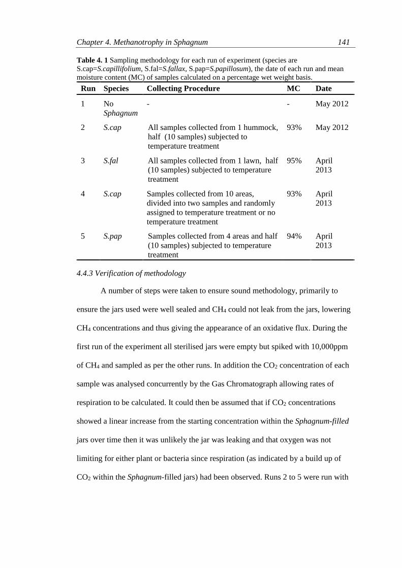
Chapter 4. Methanotrophy in Sphagnum 141
Table 4. 1 Sampling methodology for each run of experiment (species are
S.cap=S.capillifolium, S.fal=S.fallax, S.pap=S.papillosum), the date of each run and mean
moisture content (MC) of samples calculated on a percentage wet weight basis.
Run Species Collecting Procedure MC Date
1 No
Sphagnum
- - May 2012
2
S.cap
All samples collected from 1 hummock,
half (10 samples) subjected to
temperature treatment
93% May 2012
3
S.fal
All samples collected from 1 lawn, half
(10 samples) subjected to temperature
treatment
95% April
2013
4 S.cap Samples collected from 10 areas,
divided into two samples and randomly
assigned to temperature treatment or no
temperature treatment
93% April
2013
5
S.pap
Samples collected from 4 areas and half
(10 samples) subjected to temperature
treatment
94% April
2013
4.4.3 Verification of methodology
A number of steps were taken to ensure sound methodology, primarily to
ensure the jars used were well sealed and CH4 could not leak from the jars, lowering
CH4 concentrations and thus giving the appearance of an oxidative flux. During the
first run of the experiment all sterilised jars were empty but spiked with 10,000ppm
of CH4 and sampled as per the other runs. In addition the CO2 concentration of each
sample was analysed concurrently by the Gas Chromatograph allowing rates of
respiration to be calculated. It could then be assumed that if CO2 concentrations
showed a linear increase from the starting concentration within the Sphagnum-filled
jars over time then it was unlikely the jar was leaking and that oxygen was not
limiting for either plant or bacteria since respiration (as indicated by a build up of
CO2 within the Sphagnum-filled jars) had been observed. Runs 2 to 5 were run with

Chapter 4. Methanotrophy in Sphagnum 142
20 jars containing Sphagnum samples and an additional 4 Sphagnum-free jars. Runs
3 to 5 differed slightly as the 4 Sphagnum-free jars contained aluminium pieces to
aid mixing of the headspace air and CH4.
4.4.4 Calculating concentrations and oxidation rates
At each sampling time four standard samples of known CO2 and CH4
concentrations of 100.9, 5,000, 10,000 and 15,000 ppm of CH4 and 200, 344, 678
and 4941 ppm of CO2 (BOC Ltd, U.K.) were analysed before and after every 6 jar
samples. The area under each output peak (in mV) of each standard sample could
then be calculated using Clarity Chromatography Software (v.3.0.6.589). The
standard samples allowed for linear regression and calibration of the peak area
(mV.s) with the known concentrations of the four standard samples and the
subsequent calculation of the concentrations of CO2 and CH4 in the unknown jar
samples. Fluxes of both CO2 and CH4 were calculated on a jar basis as opposed to a
dry weight basis so Sphagnum-free jars could be used as a comparison using
equations 4.1 to calculate p (molar density of air in mol/m3) and 4.2 to calculate the
flux (f) where P is pressure (Pa), R is the Universal Gas Constant and T is
temperature (K), dC change in concentration, dt is change in time, and V volume.
=𝑃
𝑅 × 𝑇
Eq4. 1
𝑓 =𝑑𝐶
𝑑𝑡× 𝑝 × 𝑉
Eq4. 2

Chapter 4. Methanotrophy in Sphagnum 143
4.4.5 Statistical Analysis
One-way ANOVA’s were used to look at treatment and sampling location
effects on CH4 and CO2 fluxes with unpaired two-sample t-tests used to identify
differences between species and temperature treatment.
4.5 Results
4.5.1 CH4 Oxidation
Analysing CH4 oxidation rates over all runs of the experiment the CH4 fluxes
of Sphagnum-filled jars were not significantly different to those of Sphagnum-free
jars (Figure 4. 2). There was however considerable variation in calculated CH4 fluxes
where Sphagnum-free jars showed fluxes between -74 and +16µmol CH4 jar -1 day-1,
while Sphagnum-filled jars showed a range of between -25 to +20 µmol CH4 jar -1
day-1. These fluxes show comparatively small changes in methane concentration over
time when considering the mean initial concentration per jar measured at Time 0
across the whole experiment was 10364±50 ppm jar-1 (438±52 µmol jar-1). At a
species level CH4 fluxes were only found to be significantly lower in jars containing
S.papillosum when compared to Sphagnum-free jars from all 5 runs of the
experiment (Table 4. 2). However, when compared to the Sphagnum-free jars from
only that individual run no significant differences between treatments were found
(F(2,52)=0.01, p=0.99). No significant differences were found between burnt and
unburnt samples in any run (Figure 4. 2) and no clear relationship between CH4 fluxes
and Sphagnum dry weight detected. For the runs of the experiment which involved a
variation in sampling location, be it hummock or lawn, no statistical difference was
found in CH4 fluxes in Run4 where S.capillifolium was sampled from 10 hummocks

Chapter 4. Methanotrophy in Sphagnum 144
(F(9,8)=0.772, p=0.648), however statically different CH4 fluxes were found
between the 4 lawns where S.papillosum was sampled for Run 5 (F(3,14)=5.899,
p=0.008). However, this significant result is likely skewed by two points which
show a positive CH4 flux (Figure 4. 3).
In terms of methodological error, higher fluxes were often observed in
Sphagnum-free jars without added mixers (Figure 4. 4, Figure 4. 5). Despite this
difference not being statistically significant (t(21.8)=1.89, p=0.07) it was still
important to take this into consideration when assessing for methanotrophy in the
Sphagnum samples as when compared to empty jars without mixers there was
seemingly lower CH4 concentrations in the Sphagnum-filled jars (Figure 4. 5a). This
difference however was not seen when empty jars that did not contain mixers were
removed from the analysis (Figure 4. 5b). A number of calculated CH4 fluxes in
Sphagnum-filled jars were also removed from statistical analysis when comparing
fluxes between treatments as it was believed to be likely that there was insufficient
mixing of headspace gases leading to artificially high CH4 concentrations when
sampled at time zero and thus an over-estimated CH4 oxidation rate (Appendix 4.1).

Chapter 4. Methanotrophy in Sphagnum 145
Figure 4. 2 CH4 fluxes for each treatment (UB=unburnt, B=burnt, E=empty) per run of the
experiment. Solid vertical lines show the median, boxes the lower and upper quartiles,
whiskers the extent of upper and lower values within 1.5*inter quartile range and points
outliers. Outliers associated with assumed mixing problems not plotted (Appendix 4.1).
B
E
UB
B
E
UB
B
E
UB
B
E
UB
B
E
UB
12
34
5
-20 -10 0 10 20
mol CH4 jar1 day
1
Tre
atm
ent
Sphagnum free
S.capillifolium
S.fallax
S.capillifolium
S.papillosum

Table 4. 2 Results of One-Way ANOVA tests between all three treatments for each run of the experiment where
burnt (B) and unburnt (UB) Sphagnum-filled jars were compared to all empty (E) jars analysed across the 5 runs of
the experiment. Significant differences between groups shown in bold.
Run/Species Test Statistics Mean flux ± StError
(µmol CH4 jar -1 day-1)
1 .No Sphagnum E 0.08 ±1.04 (n=34)
2. S.capillifolium
F(2,50)=0.05, p=0.951 B -0.30±0.14 (n=10)
UB 0.40 ±0.19 (n=9)
3. S.fallax
F(2,50)=0.894, p=0.415 B 0.22 ±0.58 (n=10)
UB 2.94 ±2.91 (n=9)
4. S.capillifolium F(2,49)=1.049, p=0.358 B 0.89 ± 4.63 (n=9)
UB 4.67 ± 3.73 (n=9)
5. S.papillosum
F(2,49)=5.963, p=0.005 B 8.06 ± 3.39 (n=10)
UB 7.03 ± 3.36 (n=8)
All species F(1,72)=0.389, p=0.535 B 2.40 ± 1.43 (n=39)
UB 3.67 ± 1.43 (n=35)
Chapter 4
. Meth
anotro
phy in
Sphagnum
146

Figure 4. 3 CH4 (a) and CO2 (b) fluxes in relation to sampling location used in Runs 4 and 5 where S.capillifolium was
sampled from 10 hummocks in Run 4 and S.papillosum taken from 4 lawns in Run 5. A significant difference in both
CH4 and CO2 fluxes was found between sampling locations in Run 5 where F(3,14)=5.9, p=0.008 and F(3,14)=7.3,
p=0.004 respectively.
-20
-10
0
10
20
-20
-10
0
10
20
45
1 2 3 4 5 6 7 8 9 10
Location
mol C
H4
g1 [
dry
weig
ht]
day
1
Treatment
B
UB
50
75
100
125
50
75
100
125
45
1 2 3 4 5 6 7 8 9 10
Locationm
ol C
O2
g1 [
dry
weig
ht]
day
1
Treatment
B
UB
(a) (b) Chapter 4
. Meth
anotro
phy in
Sphagnum
147

Chapter 4. Methanotrophy in Sphagnum 148
Figure 4. 4 Conditional kernel density plot of CH4 fluxes observed in Sphagnum free jars
with (n=11) and without (n=23) the addition of mixers where dashed lines represent means.

Chapter 4. Methanotrophy in Sphagnum 149
Figure 4. 5 Boxplots (left) and conditional kernel density plots (right) of CH4 fluxes
calculated per jar per day for each temperature treatment compared to (a) all Sphagnum-free
jars and (b) only those Sphagnum-free jars containing mixers (B are burnt, UB unburnt and
E Sphagnum free jars). Dashed lines in density plot represent Treatment means and boxplot
solid lines the median, boxes the lower and upper quartiles, whiskers the extent of upper and
lower values within 1.5*inter quartile range with points outliers.
-20
0
20
B E UB
Treatment
mol C
H4
jar
1
day
1
0.000 0.025 0.050 0.075 0.100
Density
Treatment
B
E
UB
-20
0
20
B E UB
Treatment
mol C
H4
jar
1
day
1
0.000 0.025 0.050 0.075
Density
Treatment
B
E
UB
(a)
(b)
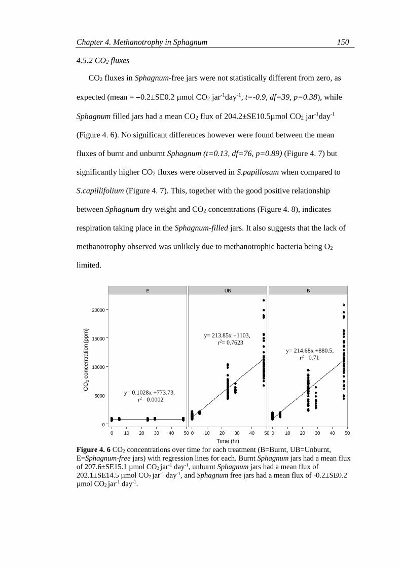
Chapter 4. Methanotrophy in Sphagnum 150
4.5.2 CO2 fluxes
CO2 fluxes in Sphagnum-free jars were not statistically different from zero, as
expected (mean = 0.2±SE0.2 µmol CO2 jar-1day-1, t=-0.9, df=39, p=0.38), while
Sphagnum filled jars had a mean CO2 flux of 204.2±SE10.5µmol CO2 jar-1day-1
(Figure 4. 6). No significant differences however were found between the mean
fluxes of burnt and unburnt Sphagnum (t=0.13, df=76, p=0.89) (Figure 4. 7) but
significantly higher CO2 fluxes were observed in S.papillosum when compared to
S.capillifolium (Figure 4. 7). This, together with the good positive relationship
between Sphagnum dry weight and CO2 concentrations (Figure 4. 8), indicates
respiration taking place in the Sphagnum-filled jars. It also suggests that the lack of
methanotrophy observed was unlikely due to methanotrophic bacteria being O2
limited.
Figure 4. 6 CO2 concentrations over time for each treatment (B=Burnt, UB=Unburnt,
E=Sphagnum-free jars) with regression lines for each. Burnt Sphagnum jars had a mean flux
of 207.6±SE15.1 µmol CO2 jar-1 day-1, unburnt Sphagnum jars had a mean flux of
202.1±SE14.5 µmol CO2 jar-1 day-1, and Sphagnum free jars had a mean flux of -0.2±SE0.2
µmol CO2 jar-1 day-1.
E UB B
0
5000
10000
15000
20000
0 10 20 30 40 50 0 10 20 30 40 50 0 10 20 30 40 50
Time (hr)
CO
2 c
on
ce
ntr
atio
n (p
pm
)
y= 0.1028x +773.73,
r2= 0.0002
y= 214.68x +880.5,
r2= 0.71
y= 213.85x +1103,
r2= 0.7623
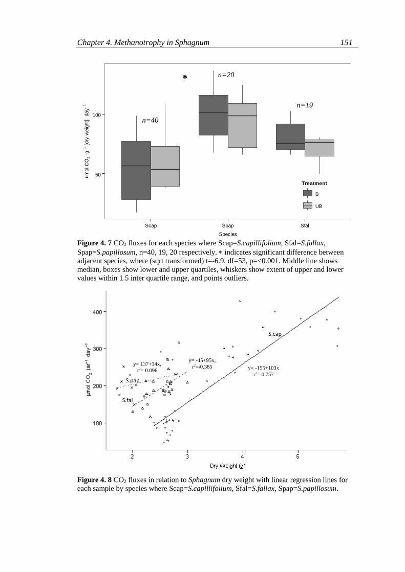
Chapter 4. Methanotrophy in Sphagnum 151
Figure 4. 7 CO2 fluxes for each species where Scap=S.capillifolium, Sfal=S.fallax,
Spap=S.papillosum, n=40, 19, 20 respectively. indicates significant difference between
adjacent species, where (sqrt transformed) t=-6.9, df=53, p=<0.001. Middle line shows
median, boxes show lower and upper quartiles, whiskers show extent of upper and lower
values within 1.5 inter quartile range, and points outliers.
Figure 4. 8 CO2 fluxes in relation to Sphagnum dry weight with linear regression lines for
each sample by species where Scap=S.capillifolium, Sfal=S.fallax, Spap=S.papillosum.
50
100
Scap Spap Sfal
Species
mol C
O2
g1 [
dry
weig
ht]
day
1
Treatment
B
UB
n=19
n=20
n=40
y= 137+34x,
r2= 0.096 y= -155+103x
r2= 0.757
y= -45+95x,
r2= 0.385
S.pap
S.fal
S.cap

Chapter 4. Methanotrophy in Sphagnum 152
4.6 Discussion
Results from the empty jars can be used to calculate a detection limit
associated with the methodology, defined here as the standard deviation in the flux in
empty jars. This gives a value of 0.08±SD6.05 µmol CH4 jar-1 day-1. Fluxes in the
Sphagnum-filled jars were mostly of a similar magnitude to this with the exception of
jars filled with S.papillosum, meaning we cannot confidently conclude that CH4
oxidation has occurred in S.capillifolium, or S.fallax. Consequently we can only
accept or reject our null hypothesis that samples subjected to the temperature
treatment would show lower CH4 oxidation rates based on our observations of
S.papillosum where we assume genuine oxidation was taking place. Within this
species no significant differences were found between burnt and unburnt samples.
Beyond these observations the results also raise important issues associated with the
methodology, a variation of which has been used in a number of studies looking at
CH4 oxidation rates in Sphagnum, and any assumptions that Sphagnum will always
host an active methanotrophic community.
4.6.1 Experimental Error
Despite being a widely used lab-based method for measuring CH4 oxidation
rates in samples of Sphagnum, the substantial number of control jars used in this
experiment suggests that there are errors associated with the experimental
procedures. The Sphagnum-free jars, representative of a Sphagnum dry weight of 0g,
gave a mean calculated CH4 flux of 0.08±SD 6.05 µmol CH4 jar-1 day-1, suggesting
that the variation of the methodology used here was not refined enough to
confidently determine genuine fluxes in Sphagnum-filled jars within the range of ±6
Chapter 4. Methanotrophy in Sphagnum 153
µmol CH4 jar-1 day-1. No significant differences in CH4 oxidation rates on a jar basis
were found between empty jars and jars filled with S.fallax or S.capillifolium, which
when corrected for dry weight showed CH4 oxidation rates of –0.6±SD2.6 and -
0.5±SD2.2µmol CH4 g [DW]1 day-1 respectively, which are within the range of
oxidation rates calculated for a number of Sphagnum species in previous studies (eg.
Basiliko et al., 2004, Raghoebarsing et al., 2005, Kip et al., 2010, Larmola et al.,
2010, Stępniewska et al., 2013) but not within the detection limit of our
methodology. The only species that could confidently be reported as exhibiting CH4
oxidation was S.papillosum which had a mean CH4 oxidation rate of -3.7
±SD4.5µmol CH4 g [DW]1 day-1 which is consistent with what has previously been
reported (Raghoebarsing et al., 2005). However, even CH4 fluxes in this species
showed considerable variation between jars and between sampling locations with
some relatively high positive fluxes recorded.
One of the sources of variation in CH4 fluxes, which could account for both
positive fluxes and the perceived CH4 oxidation in Sphagnum-free jars, could be
insufficient mixing of headspace gases, which was particularly apparent in
Sphagnum-free jars which did not contain the additional aluminium mixers. Jars with
poorly mixed headspace samples at time zero, where ambient air inside the jar did
not uniformly mix with the injected CH4, could have caused high initial CH4
concentrations and give an overall negative flux as CH4 concentrations lowered
throughout the run after the additional mixing at each sampling time. Conversely,
poorly mixed headspace samples could give rise to high CH4 concentrations being
measured at sampling times throughout each run of the experimental which could

Chapter 4. Methanotrophy in Sphagnum 154
give the false impression of CH4 being produced over time and hence positive CH4
fluxes. Positive CH4 fluxes have been recorded before using a similar methodology
and it was suggested that this could be due to small amounts of CH4 being produced
at anaerobic microsites in the Sphagnum (Basiliko et al., 2004). In this study
however positive fluxes were found in both Sphagnum-free and Sphagnum-filled jars
so it can be assumed that positive fluxes were likely due to errors associated with the
methodology. This study did use larger jars than those used by Kip et al., (2010),
Larmola et al., (2010) and Raghoebarsing et al., (2005) so insufficient mixing of the
headspace gases may be more apparent here. To compensate however for the larger
jars the Sphagnum samples were bigger to give larger, and it was hoped more
measurable, CH4 fluxes. The methodology is also inherently susceptible to apparent
CH4 oxidation actually being a product of leaking containers. However, this is not
thought to be the case here as CO2 fluxes were found to increase linearly over time in
Sphagnum-filled jars with CO2 fluxes in Sphagnum-free jars not statistically different
to zero.
4.6.2 CH4 Oxidation
The results of this experiment imply that it can only be stated with confidence
that CH4 oxidation was taking place in S.papillosum due to the large errors
associated with the methodology meaning the calculated fluxes found in S.fallax and
S.capillifolium have to be rejected. However, even if all calculated fluxes for
Sphagnum-filled jars were accepted they still show lower oxidation rates than
previously reported in the same species. S.capillifolium, a hummock forming species,
has been found to oxidise around 5 µmolCH4 g-1[DW] day-1 (Larmola et al., 2010,
Chapter 4. Methanotrophy in Sphagnum 155
Basiliko et al., 2004), while S.fallax and S.papillosum, both lawn forming species,
have been found to oxidise more than 10µmolCH4 g-1[DW] day-1 (Raghoebarsing et
al., 2005, Larmola et al., 2010). Although rates of methanotrophy are controlled by a
number of biotic and abiotic factors (Chowdhury and Dick, 2013) fundamentally at
lower atmospheric CH4 concentrations there will be lower rates of oxidation, with
artificial concentrations of CH4 greater than 10,000 ppm shown to result in the most
methanotrophy (Bender and Conrad, 1995). The concentrations used in this
experiment should therefore have promoted towards the maximum potential CH4
oxidation rates since CH4 was not limited, and so should not be responsible for the
very low oxidation observed. This leads to the assumption that the low oxidation
rates observed must be a genuine reflection of the presence/absence of
methanotrophs or environmental controls on CH4 oxidation potential in the
Sphagnum sampled.
Most research looking at the controls on methanotrophy in peatlands have
focussed on CH4 oxidation in the soil where it has been found that pH (Dunfield et
al., 1993), soil temperature (Chowdhury and Dick, 2013), soil water content (Le Mer
and Roger, 2001) and nutrient availability (Crill et al., 1994) can all affect oxidation
rates with different optimum conditions for different methanotrophs (Dunfield et al.,
2003, Dedysh et al., 2000). However, it is the position of the water table which
ultimately determines the extent of the aerobic zone and a CH4 oxidation gradient
which exists downwards in the peat layer (Sundh et al., 1995). In Sphagnum
dominated areas of a tundra bog it has been shown that most oxidation occurs at the
interface between the peat and Sphagnum layers (Vecherskaya et al., 1993) where

Chapter 4. Methanotrophy in Sphagnum 156
the optimum O2:CH4 ratio exists (Chowdhury and Dick, 2013). Less is understood
about the controls on methanotrophy in Sphagnum above this interface but the
position of the water table has been found to be particularly important for CH4
oxidation (Larmola et al., 2010) linking rates of oxidation to microhabitat and
species.
Sphagnum species associated with pools tend to show much larger potential
rates of CH4 oxidation than lawn or hummock species (Larmola et al., 2010, Kip et
al., 2010, Raghoebarsing et al., 2005), with an increase in the distance between the
moss layer and water table being negatively correlated with CH4 oxidation (Basiliko
et al., 2004). However, the lowering of the water table and the associated reduction
in CH4 oxidation (Basiliko et al., 2004, Larmola et al., 2010) may not necessarily
reduce CH4 oxidation in the long term as methanotrophic bacteria can re-colonise
Sphagnum from surrounding water when re-wetted (Putkinen et al., 2012). There
were no periods of drought prior to sampling the Sphagnum used in this experiment
with Sphagnum sampled at a field moisture content of between 93 and 95% which
suggests that low rates of CH4 oxidation were not related to low precipitation and
change in moisture status as has been found before (Basiliko et al., 2004, Larmola et
al., 2010). Seasonal effects, be it position of the water table or temperature, on
oxidation rates cannot, however, be verified by this study since all samples came
from spring months with similar temperature and water table conditions. In addition
to the abiotic controls on CH4 oxidation, which may vary temporally and spatially
across a bog, rates of oxidation may also change at a much smaller scale within
Sphagnum plants themselves.

Chapter 4. Methanotrophy in Sphagnum 157
Sphagnum grows from the top of its stem (capitulum) and naturally breaks
down from the bottom (Clymo and Hayward, 1982) leading to stems which change
in physical and biological characteristics along their length. Lower oxidation rates
have been associated with the top and middle parts of stems of the non-submerged
lawn species S. papillosum and Sphagnum magellanicum Brid. (Raghoebarsing et
al., 2005) with significantly higher CH4 oxidation found in the lower segments of the
stems with a loss in physical structure in S.capillifolium and S.magellanicum
(Basiliko et al., 2004). The rate of CH4 oxidation however may also be influenced by
habitat, namely if a plant is submerged or not submerged, as demonstrated in
Sphagnum fallax (H.Klinggr.) H.Klinggr. by Stepniewska et al., (2013) where in
contrast the highest oxidation rates were in the top parts of the stem. This change in
oxidation rate along stems could perhaps account for low the CH4 oxidation found in
this study, as only the top, more physically intact, 5cm of Sphagnum was sampled.
Oxidation rates measured here are indeed more comparable to those of the upper
parts of stems of lawn forming S.magellanicum and S.papillosum found by
Raghoebarsing et al., (2005).
4.7 Conclusions and Future Research
The results of this experiment suggest that inherent methodological errors can
be responsible for an over estimation of CH4 oxidation rates using closed flasks with
artificial CH4 concentrations, shown here by the negative CH4 fluxes recorded in
Sphagnum-free jars. This highlights the need for the methodology to be rigorously
tested and the need to include more controls, specifically empty flasks, as part of the
experiment. However, the problems found here with insufficient mixing may be
Chapter 4. Methanotrophy in Sphagnum 158
associated with the large size of the flasks used as its not been reported as a problem
in previous studies using smaller flasks.
Due to the errors in the methodology the very low oxidation rates found in
S.fallax and S.capillifolium cannot be accepted and leads to an assumption that it is
just as likely that no oxidation was occurring in these species. S.papillosum was the
only species to exhibit CH4 oxidation, meaning hypothesis [1] can be accepted as
oxidation rates were found to differ between species. As S.papillosum was the only
species to show CH4 oxidation it was the only species in which hypothesis [2] could
be tested and showed no significant difference in rates of CH4 oxidation in burnt and
unburnt Sphagnum leading to a rejection of hypothesis [2] in this instance. This
finding would have to be further tested, particularly between species, as differences
in pre-treatment moisture content and differences in morphology between species
could be important in determining the full effect of fire on the methanotrophic
community in Sphagnum. The role of methanotrophs is increasingly being
recognised for their significance to the carbon balance of peatlands and if fire were
found to have a negative impact on CH4 oxidation rates it could better inform best
practice management guidelines and carbon budget models. However it is also
important to extend the research to look at the long term impact of fire on the
methanotrophic community and rates of CH4 oxidation in the Sphagnum layer in situ
as the re-colonisation of Sphagnum by methanotrophs in the surrounding water
(Putkinen et al., 2012) could negate any initial impact of fire.

Chapter 4. Methanotrophy in Sphagnum 159
4.8 References
ANDERSEN, R., CHAPMAN, S. J. & ARTZ, R. R. E. 2013. Microbial communities
in natural and disturbed peatlands: A review. Soil Biology and Biochemistry,
57, 979-994.
BASILIKO, N., KNOWLES, R. & MOORE, T. 2004. Roles of moss species and
habitat in methane consumption potential in a northern peatland. Wetlands,
24, 178-185.
BENDER, M. & CONRAD, R. 1995. Effect of CH4 concentrations and soil
conditions on the induction of CH4 oxidation activity. Soil Biology and
Biochemistry, 27, 1517-1527.
BUTLER, J. 2012. The NOAA Annual Greenhouse Gas Index (AGGI) [Online].
Earth System Research Laboratory: Global Monitoring Dvision Website.
[Accessed 08/07/2013 2013].
CHEN, Y., DUMONT, M. G., MCNAMARA, N. P., CHAMBERLAIN, P. M.,
BODROSSY, L., STRALIS-PAVESE, N. & MURRELL, J. C. 2008.
Diversity of the active methanotrophic community in acidic peatlands as
assessed by mRNA and SIP-PLFA analyses. Environmental Microbiology,
10, 446-459.
CHEN, Y. & MURRELL, J. C. 2010. Geomicrobiology: Methanotrophs in moss.
Nature Geosci, 3, 595-596.
CHOWDHURY, T. R. & DICK, R. P. 2013. Ecology of aerobic methanotrophs in
controlling methane fluxes from wetlands. Applied Soil Ecology, 65, 8-22.
CLYMO, R. S. & HAYWARD, P. M. 1982. The Ecology of Sphagnum In: SMITH,
A. J. E. (ed.) Bryophyte Ecology. New York: Chapman and Hall Ltd.
CRILL, P. M., MARTIKAINEN, P. J., NYKA ̋NEN, H. & SILVOLA, J. 1994.
Temperature and N fertilization effects on methane oxidation in a drained
peatland soil. Soil Biology and Biochemistry, 26, 1331-1339.
DAVIES, G. M. 2005. Fire behaviour and impact on heather moorland. Ph.D,
University of Edinburgh.
DEDYSH, S. N., LIESACK, W., KHMELENINA, V. N., SUZINA, N. E.,
TROTSENKO, Y. A., SEMRAU, J. D., BARES, A. M., PANIKOV, N. S. &
TIEDJE, J. M. 2000. Methylocella palustris gen. nov., sp. nov., a new
methane-oxidizing acidophilic bacterium from peat bogs, representing a
novel subtype of serine-pathway methanotrophs. Int J Syst Evol Microbiol, 50
Pt 3, 955-69.

Chapter 4. Methanotrophy in Sphagnum 160
DUNFIELD, P., KNOWLES, R., DUMONT, R. & MOORE, T. R. 1993. Methane
production and consumption in temperate and subarctic peat soils: Response
to temperature and pH. Soil Biology and Biochemistry, 25, 321-326.
DUNFIELD, P. F., KHMELENINA, V. N., SUZINA, N. E., TROTSENKO, Y. A. &
DEDYSH, S. N. 2003. Methylocella silvestris sp. nov., a novel methanotroph
isolated from an acidic forest cambisol. Int J Syst Evol Microbiol, 53, 1231-9.
GLIME, J. M. 2007. Physiological Ecology. Bryophyte Ecology. Ebook sponsored
by Michigan Technological University and the International Association of
Bryologists.
GORHAM, E. 1991. Northern Peatlands - Role in the Carbon-Cycle and Probable
Responses to Climatic Warming. Ecological Applications, 1, 182-195.
GUPTA, V., SMEMO, K. A., YAVITT, J. B., FOWLE, D., BRANFIREUN, B. &
BASILIKO, N. 2013. Stable Isotopes Reveal Widespread Anaerobic Methane
Oxidation Across Latitude and Peatland Type. Environmental Science &
Technology.
HANSON, R. S. & HANSON, T. E. 1996. Methanotrophic bacteria. Microbiological
Reviews, 60, 439-71.
IPCC 2013. Working Group I Contribution to the IPCC Fifth Assessment Report
(AR5), Climate Change 2013: The Physical Science Basis., Geneva,
Switzerland, Intergovernmental Panel on Climate Change.
KIP, N., VAN WINDEN, J. F., PAN, Y., BODROSSY, L., REICHART, G.-J.,
SMOLDERS, A. J. P., JETTEN, M. S. M., DAMSTE, J. S. S. & OP DEN
CAMP, H. J. M. 2010. Global prevalence of methane oxidation by symbiotic
bacteria in peat-moss ecosystems. Nature Geosci, 3, 617-621.
LARMOLA, T., TUITTILA, E.-S., TIIROLA, M., NYKÄNEN, H.,
MARTIKAINEN, P. J., YRJÄLÄ, K., TUOMIVIRTA, T. & FRITZE, H.
2010. The role of Sphagnum mosses in the methane cycling of a boreal mire.
Ecology, 91, 2356-2365.
LE MER, J. & ROGER, P. 2001. Production, oxidation, emission and consumption
of methane by soils: A review. European Journal of Soil Biology, 37, 25-50.
NYKÄNEN, H., ALM, J., SILVOLA, J., TOLONEN, K. & MARTIKAINEN, P. J.
1998. Methane fluxes on boreal peatlands of different fertility and the effect
of long-term experimental lowering of the water table on flux rates. Global
Biogeochemical Cycles, 12, 53-69.
PARMENTIER, F. J. W., VAN HUISSTEDEN, J., KIP, N., OP DEN CAMP, H. J.
M., JETTEN, M. S. M., MAXIMOV, T. C. & DOLMAN, A. J. 2011. The
role of endophytic methane-oxidizing bacteria in submerged Sphagnum in

Chapter 4. Methanotrophy in Sphagnum 161
determining methane emissions of Northeastern Siberian tundra.
Biogeosciences, 8, 1267-1278.
PUTKINEN, A., LARMOLA, T., TUOMIVIRTA, T., SILJANEN, H. M.,
BODROSSY, L., TUITTILA, E.-S. & FRITZE, H. 2012. Water dispersal of
methanotrophic bacteria maintains functional methane oxidation in
Sphagnum mosses. Frontiers in Microbiology, 3.
RAGHOEBARSING, A. A., SMOLDERS, A. J. P., SCHMID, M. C., RIJPSTRA,
W. I. C., WOLTERS-ARTS, M., DERKSEN, J., JETTEN, M. S. M.,
SCHOUTEN, S., SINNINGHE DAMSTE, J. S., LAMERS, L. P. M.,
ROELOFS, J. G. M., OP DEN CAMP, H. J. M. & STROUS, M. 2005.
Methanotrophic symbionts provide carbon for photosynthesis in peat bogs.
Nature, 436, 1153-1156.
SHEPPARD, L. J., LEITH, I. D., LEESON, S. R., VAN DIJK, N., FIELD, C. &
LEVY, P. 2012. Fate of N in a peatland, Whim bog: N immobilisation in the
vegetation and peat, leakage into pore water and losses as N2O depend on the
form of N. Biogeosciences Discuss., 9, 8141-8171.
SHEPPARD, L. J., LEITH, I. D., MIZUNUMA, T., LEESON, S., KIVIMAKI, S.,
NEIL CAPE, J., VAN DIJK, N., LEAVER, D., SUTTON, M. A., FOWLER,
D., VAN DEN BERG, L. J. L., CROSSLEY, A., FIELD, C. & SMART, S.
2014. Inertia in an ombrotrophic bog ecosystem in response to 9 years'
realistic perturbation by wet deposition of nitrogen, separated by form.
Global Change Biology, 20, 566-580.
SINGH, B. K., BARDGETT, R. D., SMITH, P. & REAY, D. S. 2010.
Microorganisms and climate change: terrestrial feedbacks and mitigation
options. Nat Rev Micro, 8, 779-790.
STĘPNIEWSKA, Z., KUŹNIAR, A., PYTLAK, A. & SZYMCZYCHA, J. 2013.
Detection of methanotrophic endosymbionts in Sphagnum sp. originating
from Moszne peat bog (East Poland). African Journal of Microbiology
Research 7, 1319-1325.
SUNDH, I., MIKKELÄ, C., NILSSON, M. & SVENSSON, B. H. 1995. Potential
aerobic methane oxidation in a Sphagnum-dominated peatland—Controlling
factors and relation to methane emission. Soil Biology and Biochemistry, 27,
829-837.
VECHERSKAYA, M. S., GALCHENKO, V. F., SOKOLOVA, E. N. &
SAMARKIN, V. A. 1993. Activity and species composition of aerobic
methanotrophic communities in tundra soils. Current Microbiology, 27, 181-
184.

Chapter 4. Methanotrophy in Sphagnum 162
WHALEN, S. C. 2005. Biogeochemistry of Methane Exchange between Natural
Wetlands and the Atmosphere. Environmental Engineering Science, 22, 73-
94.
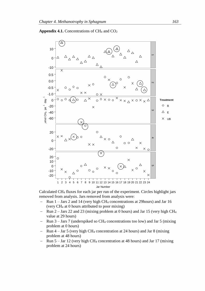
Chapter 4. Methanotrophy in Sphagnum 163
Appendix 4.1. Concentrations of CH4 and CO2
Calculated CH4 fluxes for each jar per run of the experiment. Circles highlight jars
removed from analysis. Jars removed from analysis were:
Run 1 – Jars 2 and 14 (very high CH4 concentrations at 29hours) and Jar 16
(very CH4 at 0 hours attributed to poor mixing)
Run 2 – Jars 22 and 23 (mixing problem at 0 hours) and Jar 15 (very high CH4
value at 29 hours)
Run 3 – Jars 7 (underspiked so CH4 concentrations too low) and Jar 5 (mixing
problem at 0 hours)
Run 4 – Jar 5 (very high CH4 concentration at 24 hours) and Jar 8 (mixing
problem at 48 hours)
Run 5 – Jar 12 (very high CH4 concentration at 48 hours) and Jar 17 (mixing
problem at 24 hours)
-10
0
10
-1.0
-0.5
0.0
0.5
-60
-40
-20
0
-20
0
20
-20
-10
0
10
20
12
34
5
1 2 3 4 5 6 7 8 9 10 11 12 13 14 15 16 17 18 19 20 21 22 23 24
Jar Number
mol C
H4
jar
1
day
1
Treatment
B
E
UB
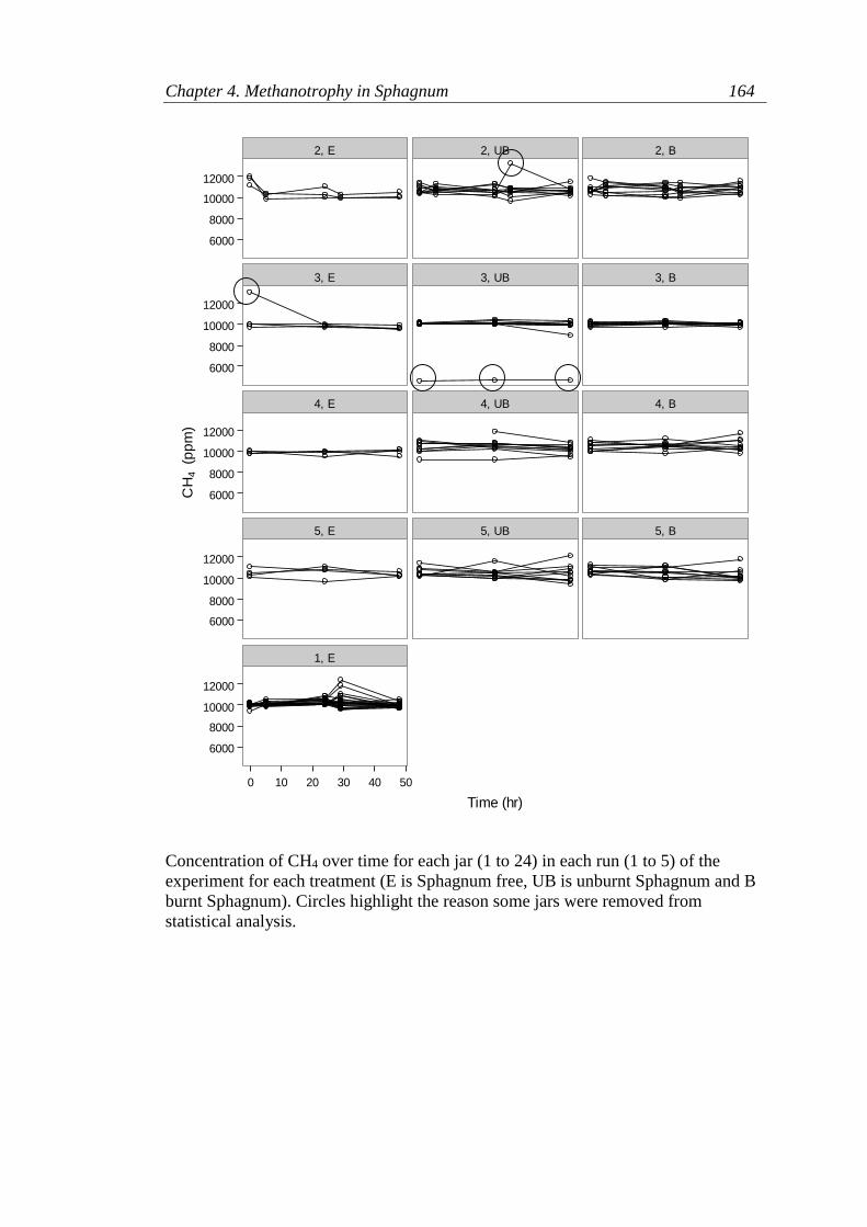
Chapter 4. Methanotrophy in Sphagnum 164
Concentration of CH4 over time for each jar (1 to 24) in each run (1 to 5) of the
experiment for each treatment (E is Sphagnum free, UB is unburnt Sphagnum and B
burnt Sphagnum). Circles highlight the reason some jars were removed from
statistical analysis.
2, E 2, UB 2, B
3, E 3, UB 3, B
4, E 4, UB 4, B
5, E 5, UB 5, B
1, E
6000
8000
10000
12000
6000
8000
10000
12000
6000
8000
10000
12000
6000
8000
10000
12000
6000
8000
10000
12000
0 10 20 30 40 50
Time (hr)
CH
4 (p
pm
)

Chapter 4. Methanotrophy in Sphagnum 165
Concentration of CO2 over time for each jar (1 to 24) in each run (1 to 5) of the
experiment for each treatment (E is Sphagnum free, UB is unburnt Sphagnum and B
burnt Sphagnum). All jars were kept in the statistical analysis of CO2 fluxes.
2, E 2, UB 2, B
3, E 3, UB 3, B
4, E 4, UB 4, B
5, E 5, UB 5, B
1, E
0
5000
10000
15000
20000
0
5000
10000
15000
20000
0
5000
10000
15000
20000
0
5000
10000
15000
20000
0
5000
10000
15000
20000
0 10 20 30 40 50
Time (hr)
CO
2 (p
pm
)

Chapter 5. Burning and Vegetation 166
5. The impact of burning on vegetation of three blanket bogs in
Scotland
5.1 Abstract
In the UK fire is used as a tool to manage vegetation for livestock and grouse,
and blanket bog can be burned in special circumstances under existing legislation
and best practice guidance. Burning, however, has the potential to cause the loss of
fire sensitive species and modify processes such as carbon cycling and peat
formation. The aim of this study was to look at the changes in vegetation brought
about by low severity fire events, which burned only the canopy vegetation and did
not penetrate the peat, at three blanket bogs in Scotland. To further assess the impact
these fires had on the critical Sphagnum layer, Sphagnum capillifolium was
monitored to quantify any reduction and recovery in photosynthetic capacity. The
results show that the fires caused the dominance of graminoids over shrubs, which is
consistent with the literature, and that this was to some degree reflected in National
Vegetation Classification classifications. Changes in vegetation composition could
be linked to both fire severity and time since burning. The photosynthetic capacity of
the capitula of S.capillifolium was reduced by burning for over two years after the
fire events, but this was shown to be less critical in some instances in the long term
as some damaged stems had the capacity to grow new healthy stem and capitula.
These results show that even low severity fires have the potential to change
vegetation composition for a number of years after burning and that the impact on
the Sphagnum layer can vary at the micro-scale. The results also reiterate that fire is

Chapter 5. Burning and Vegetation 167
highly variable in its impacts and will have different implications for vegetation
depending on pre-burn vegetation composition, age and structure, and fire behaviour.
5.2 Introduction
The impact of fire on the vegetation of peatlands in the UK is best understood
in the context of Calluna vulgaris (L.) Hull (from here expressed as Calluna)
dominated heaths, primarily due to the need to inform management on grouse moors.
Traditionally heather is burned to encourage new more palatable growth and
structural diversity as in the right circumstances Calluna, a low growing perennial
shrub, responds to fire by putting up new shoots or growing from new seed. The age
at which Calluna heaths are burned is important as older plants have been found to
have less capacity for vegetative growth (Miller and Miles 1970). The length of the
burning rotation is therefore important in ensuring optimal heather regeneration and
since the early 20th century rotation periods and optimum burn sizes have been
prescribed for heather dominated heaths on this basis (eg. Lovat, 1911, Gimingham,
1972). The Muirburn Code for Scotland, for instance, has based best practice rotation
times directly on the amount of annual growth of Calluna (Scottish Executive, 2011).
Fire has, however, also long been used to deliberately manipulate vegetation
composition in the long term, promoting more palatable graminoids over older
shrubs. Understanding the response of vegetation to fire on blanket bog is therefore
an important consideration when aiming to maintain blanket bogs as an important
habitat and carbon store with best practice burning guidelines.
Previous reviews have shown that the impact of burning blanket bog, in the
context of the Joint Nature Conservations Committees defined “favourable
Chapter 5. Burning and Vegetation 168
condition” (Joint Nature Conservation Committee, 2006), is contradictory, with
species composition change being both either a positive or negative deviation from
favourable condition (Stewart et al., 2004) with little empirical evidence for fire
having a damaging effect on blanket bogs (Stewart et al., 2005). However, common
observations are that fire can promote the dominance of a small number of species,
lead to an increase in bare ground and result in a change in abundance of species, the
majority of datasets showing a decrease in abundance of key species (Stewart et al.,
2004). Graminoids such as Eriophorum spp. (Rawes and Hobbs, 1979, Stewart et al.,
2004, Gray, 2006, Ward et al., 2007) and Molinia caerulea (Hamilton, 2000, Ross et
al., 2003) can increase in abundance over Calluna following burning. However, the
frequency of burning has been demonstrated to be an important factor in facilitating
long term changes in species composition (Gray 2006), with 10 year rotations having
a greater effect than 20 year rotations (Rawes and Hobbs, 1979) with shorter
rotations favouring graminoids (Lee et al., 2013).
A plant’s ability to recover from a fire will be related to its physiology and
pre and post burn environmental conditions, which in turn can be related to fire
behaviour and severity. Regeneration may relate to the life histories of the pre-burn
plant community, and can be dependant on the timing of critical stages in a plants
growth cycle in relation to the timing of a fire event (Mallik and Gimingham, 1983,
Hobbs et al., 1984). Fire behaviour and the temperature gradient found in a fire also
have implications for vegetation recovery, with lower ground surface temperatures
important for Calluna regeneration form lateral meristems at the stem base after fire
(Kayll, 1966), and the temperature below ground important when considering seed

Chapter 5. Burning and Vegetation 169
banks and seed viability within the soil. Schimmel and Granstrom (1996) for
example demonstrated that plant survival following experimental burning of
understory vegetation in a Boreal pine forest in Sweden, at sites dominated by
Vaccinium vitis-idaea L., Vaccinium myrtillus L. and Deschampsia cespitosa (L.)
P.Beauv. was dependant on the depth to which temperatures increased below ground
in a fire, and the depth within the soil that plants held regenerative structure. This
supports observations of wildfires in the UK where regeneration of blanket bog
vegetation in areas which were severely scorched and turned to ash, indicative of
burns where high temperatures penetrated deeper into the peat layer (Ashton et al.,
2007), showed little or no recovery (Maltby et al., 1990). Post fire input of nutrients
from ash deposition (Allen, 1964) and the reduction in competition may also favour
some more competitive species over others. In addition, confounding the effect of
fire is the relationship between burning and grazing as post fire grazing pressure may
increase (Hamilton, 2000), resulting in a cumulative management effect which may
have wider implications such as soil compaction (Gray, 2006).
5.3 Aims
The aim of this study was to increase our understanding of the effects of fire
on vegetation composition of blanket bogs by assessing how fire changed the
vegetation composition in the short to medium term (months to 3 years). It was also
intended that any changes in species composition over this timescale be considered
in relation to CH4 emissions and ecosystem respiration measured at the same plots
(see Chapter 2). Species composition was assessed over time to determine how the
change in vegetation composition related to the time since burning and to see if there
Chapter 5. Burning and Vegetation 170
were trends in plant succession at different sites. Species composition was also
matched to National Vegetation Classification (NVC) communities (Elkington et al.,
2001) to examine if this method of classification, used widely by ecologists, could
sufficiently show the short term change in vegetation community brought about by
burning. Previously there has been some doubt whether this system is appropriate for
showing the effects of fire on vegetation composition (Gray, 2006). In addition, and
in response to the limited information available on how Sphagnum is affected by
burning (as discussed in Chapter 3), the surface of lawns and hummocks of
Sphagnum capillifolium (Ehrh.) Hedw. at each site were assessed with a specific
measure of photosynthetic capacity, chlorophyll fluorescence, to quantify impacts
and show any recovery.
It was hypothesised that [1], although there would be differences in species
composition between the three sites, there would be a common trend of fire
increasing the abundance of graminoid species, while reducing shrub cover in the
short term but in the medium term promoting the growth of new shrub plants. That
[2] the differences between the vegetation communities of the burnt plots and
unburnt reference plots would be reflected in NVC classifications. In regards to the
effect of fire on S.capillifolium it was hypothesised that [3] the capitula, when not
entirely consumed, would show a long term reduction in photosynthetic capacity due
to physiologically lethal temperatures being reached at the moss surface during the
fires, with recovery slow and dependent on new regenerative growth.
Chapter 5. Burning and Vegetation 171
5.4 Methodology
5.4.1 Site description and survey methodology
The plots used in this study were the same as those used for sampling CO2
and CH4 (described in Chapter 2) as samples were taken using a closed chamber
system. This meant a permanent circular collar, 43cm in diameter, remained in-situ
for the duration of the study period, providing a constant area to monitor species
composition. However, the vegetation assessment needed to cause minimal
disturbance within each collar for the natural CO2 and CH4 fluxes to be measured.
Therefore, percentage top cover of each species was assessed throughout the duration
of the study while harvesting of the vegetation within each collar and total percent
cover and dry weight only calculated when flux measurements had ceased. By
concurrently monitoring unburnt plots at each site, the change in vegetation in the
burnt plots over time could be compared to control plots to give an indication of
recovery to pre-burn composition.
As described in Chapter 2 each site had been subjected to a fire; two for
management purposes and one by an accidental wildfire, and an equal number of
plots were located either side of the fire line at each site to allow for comparisons to
be made between burnt plots and unburnt reference plots (Table 5. 1). The fires at all
sites were similar in character, mostly only removing the canopy vegetation of
graminoids and Calluna vulgaris (L.) Hull (from here expressed as Calluna) while
not penetrating the peat. The moss layer was only consumed in small discrete areas,
with the drier pleurocarpous and acrocarpous mosses suffering more damage than
Sphagnum species. The fire at Glensaugh removed the least amount of biomass, with
Chapter 5. Burning and Vegetation 172
the finer branches of Calluna left intact in places, compared to mostly just the woody
stems of Calluna remaining after the fires at Eastside and Forsinard (Appendix 2.1).
Fuel loads, as indicated from the harvesting of 6 unburnt plots adjacent to the areas
burned at Forsinard and Eastside, showed that Eastside was characterised by a much
greater dry weight of shrubs, predominantly Calluna, when compared to Forsinard
although total graminoid and sedge biomass were similar (Chapter 2, Table 2.2).
Glensaugh was similar to Eastside in terms of vegetation composition and structure,
with similar Calluna biomass at the time of burning.
5.4.2 Percentage top cover assessment
Digital photographs were taken of each plot throughout the study period to
show changes in vegetation composition. However, images from only three time
points at each site were used in the analysis, as often the images were of poor quality
due to low light levels and weather conditions making identification to an individual
species level difficult. Since each area within the collars being monitored was
circular, images of each plot were assessed digitally with an 8 sector grid
superimposed onto each image (Figure 5. 1). The total area of each plot was
1452cm2, with each 8 sector segment covering 363cm2. This meant percentage top
cover could be assessed in each of the 8 sectors more easily by eye, and combined to
give a more accurate estimation of the whole plot. Each species was identified non-
destructively in the field or from a representative specimen taken from areas adjacent
from the plots if more comprehensive identification was needed.

Table 5. 1 Vegetation survey site descriptions (See Appendix 2.1 for maps and images of the sites). M measured, 1Levy et al. (2012), 2Centre for Ecology and Hydrology (2012), 3Ball et al. (2012) , 4UK Environmental Change Network (2012).
Site Name Grid Ref Date of Burn Plots Surveyed
Mea
n S
T
(oC
)
Mea
n
Pre
cip
itati
on
(mm
/yr)
Alt
itu
de
(m
above
sea
level
)
Slo
pe (
o)
Asp
ect
East
ing
Nort
hin
g
Forsinard
NC 884 408 18/04/2011
6 Burned,
6 Unburned
9.2 M 825 2 190 0.6 S 288450 940850
Eastside
NT 162 602
14/03/2012 7 Burned,
7 Unburned
7.3 M 789 3 420 2 SE 316250 660250
Glensaugh NO 664 810 27/03/2012 4 Burned,
4 Unburned
7.3 1 1130 4 410 9 N 366450 781050
Chapter 5
. Burn
ing a
nd V
egeta
tion
1
73

Chapter 5. Burning and Vegetation 174
Figure 5. 1 Example image of a plot where percentage top cover of each plant
species was surveyed, showing the superimposed digital 8-sector layer to aid
assessment.
5.4.3 Total percentage cover and dry weight
On the last day of flux measurements each plot was surveyed, by eye, in the
field for total percentage cover of each species. This gave a summed total percent
cover of all species >100% as opposed the top cover survey which gave a maximum
100%. Once surveyed each plot was harvested by removing all vegetation above the
peat layer and sorted into each species component. Each harvested species was dried
at 70oC for up to 7 days (or when weight was no longer decreasing) to achieve a dry
weight for each species. Species lists for each of the three sites can be found in
Appendix 5.1. Small fragments of vegetation and longer lengths of dead graminoids

Chapter 5. Burning and Vegetation 175
were considered “litter”. Calluna was further sorted into woody stems and finer
branch material.
The vegetation community at each site in the burnt and unburnt plots were
attributed to NVC sub communities (Elkington et al., 2001) using the NVC
classification software ComKey (Legg, 2008). Plots were split into burnt and unburnt
communities for each sampling time per site and matched to an NVC community by:
matching species, counting the number of species which occurred in the matched
community, by a weighted species match which, in addition to counting the number
of species occurring in the matched community species were given weight according
to their fidelity, and finally by frequency weighted match which accumulated scores
for species common with matched community weighted by the fidelity of the species.
The community which ranked #1 for each match method was chosen, however,
results were sense checked with the literature (Rodwell, 1991, Elkington et al., 2001)
to ensure matched communities were appropriate. NVC classifications were also
compared between the top cover survey method, employed throughout the study
period, and the full survey method used on the final day of sampling to show if the
top cover survey underestimated cover of any species.
5.4.4 Assessment of Sphagnum recovery
To assess the effect the fires had on Sphagnum recovery photosynthetic
capacity was estimated using chlorophyll fluorescence as an indicator of Sphagnum
health. Chlorophyll fluorescence is a technique that has been widely used to assess
recovery in Sphagnum following stress (eg. van Gaalen et al., 2007, Hájek and
Chapter 5. Burning and Vegetation 176
Beckett, 2008, Manninen et al., 2011). A more detailed account of the technique is
given in Chapter 3 (section 3.4.2.1).
Measurements were made on Sphagnum capillifolium (Ehrh.) Hedw. a
widespread species in the UK, and common to all three field sites. At each site
measurements were made on the capitula of plants from the burnt area and
concurrently from the adjacent unburnt area. Sampling design did vary between sites
as S.capillifolium abundance and the number and size of fires varied making a
consistent sampling design difficult (Table 5. 2). Due to the small size of the fires
and lower abundance of Sphagnum spp. at Eastside, S.capillifolium was sampled
from three hummocks from a total of three different fires (each however were burned
only minutes apart on the same day in the same weather conditions), with unburnt
S.capillifolium sampled from an adjacent unburnt area. At Forsinard, where
vegetation was more uniform with Sphagnum spp. found throughout, 10 discrete
patches of S.capillifolium were identified both sides of the fire line in the same area.
At Glensaugh five sampling areas were identified along a transect through the burnt
area and unburnt S.capillifolium sampled from the adjacent unburnt area.
Measurements were always made on the capitula of stems taken from the same
sampling locations. However, due to the destructive nature of the technique
measurements were not made on the same stems at each sampling time. Prior to
making each fluorescence measurement, made at a light intensity of 1,500 µmol m-2
s-1, each capitula (3 per sampling location) were dark adapted for 20 minutes using a
dark adaption clip (HPEA/LC, Hansatech Instruments Ltd, UK). Samples from each
hummock/lawn area were also removed for moisture content analysis, each sample

Chapter 5. Burning and Vegetation 177
being weighed prior to being oven dried at 70oC for 1 week, after which the sample
was weighed again and moisture content (MC), on a percentage wet weight basis,
calculated using equation 5.1 where w is wet weight, and d is dry weight.
𝑀𝐶 =𝑤 − 𝑑
𝑤 × 100
Eq 5. 1
Table 5. 2 Sampling procedure for chlorophyll fluorescence measurements at each field site
where S.capillifolium was sampled from hummocks or areas of lawn at various time points
after the site was burnt.
Site Name Fire Sampling
Location
Total number
of capitula
sampled/site
Time period
sampled (number
days since fire)
Forsinard
1
10 burnt
10 unburnt
60
38 -766
Eastside
1
2
3
3 burnt
3 burnt
3 burnt
3 unburnt
36 5 - 439
Glensaugh 1 5 burnt
5 unburnt 30 81 - 440
5.4.5 Statistical Analysis
5.4.5.1 Analysis I
To investigate if there were significant site level differences in species
composition an unconstrained detrended correspondence analysis (DCA) using
CANOCO 5 (ter Braak and Šmilauer, 2012) was used on the total percentage cover

Chapter 5. Burning and Vegetation 178
data from the final day of sampling. The environmental terms soil temperature (ST),
mean soil moisture (SM) and mean height of the water table (WT), which had all
been measured at a plot level over the duration of the study period, with the
exception of WT at Glensaugh which had been calculated from SM (Appendix 2.2),
were plotted as supplementary variables. A detailed account of how these
measurements were made is given in Chapter 2 (section 2.4.2). Plotting the
environmental variables as supplementary variables allowed for a projection of the
environmental variables onto the species data, without influencing the species and
sample ordination which would be problematic due to the unbalanced experimental
design (some sites sampled more than others) and repeated measures (samples from
same plots over time). To further assess the differences between the three sites, mean
precipitation, altitude, steepness of slope, aspect and location (easting/northing) were
also included in the DCA. The plotted ordination diagram of the DCA results allow
the dissimilarity of distribution of species to be evaluated, the closer the species are
plotted on the ordination diagram the more often they occur together. The DCA
ordination diagram can also show the dissimilarity between environmental variables
in the same way. The continuous environmental variables are plotted as arrows in the
direction of the steepest increase in value and show the marginal effects of the
environmental variable upon species sample scores.
5.4.5.2 Analysis II
To assess the differences between burnt and unburnt vegetation communities
at each site and how species composition changed in the burnt plots over time
Principle Response Curves (PRC), a multivariate constrained ordination approach
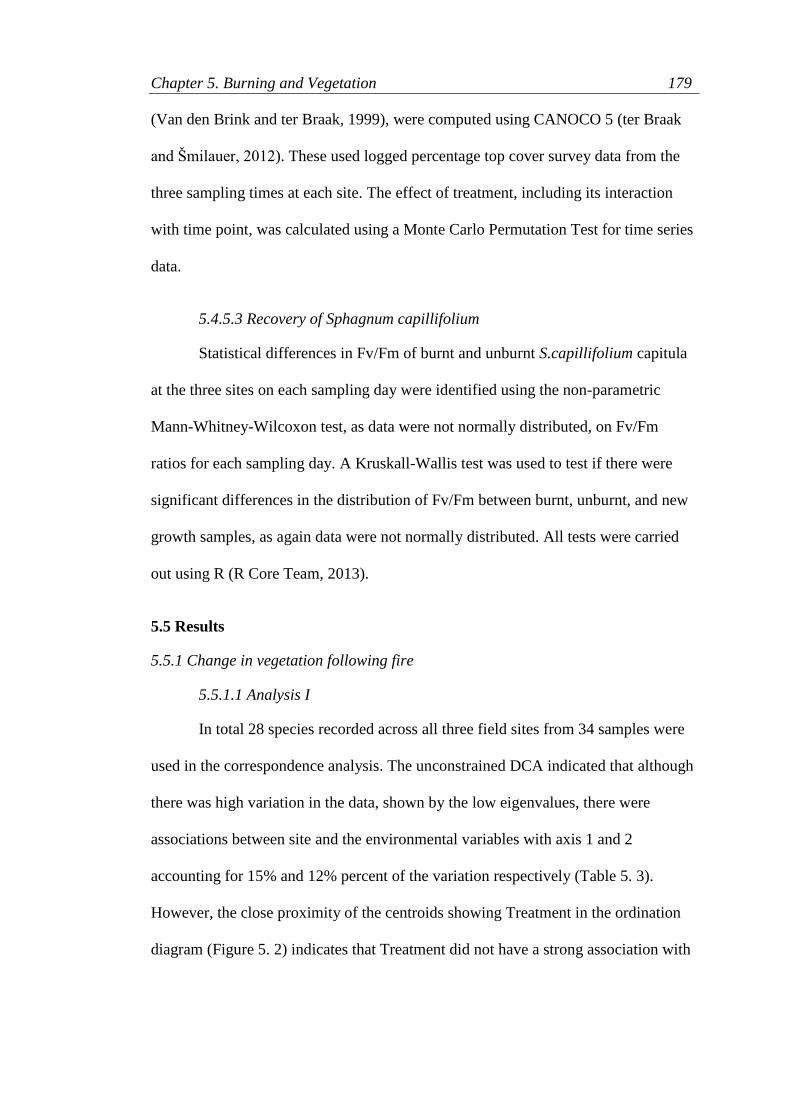
Chapter 5. Burning and Vegetation 179
(Van den Brink and ter Braak, 1999), were computed using CANOCO 5 (ter Braak
and Šmilauer, 2012). These used logged percentage top cover survey data from the
three sampling times at each site. The effect of treatment, including its interaction
with time point, was calculated using a Monte Carlo Permutation Test for time series
data.
5.4.5.3 Recovery of Sphagnum capillifolium
Statistical differences in Fv/Fm of burnt and unburnt S.capillifolium capitula
at the three sites on each sampling day were identified using the non-parametric
Mann-Whitney-Wilcoxon test, as data were not normally distributed, on Fv/Fm
ratios for each sampling day. A Kruskall-Wallis test was used to test if there were
significant differences in the distribution of Fv/Fm between burnt, unburnt, and new
growth samples, as again data were not normally distributed. All tests were carried
out using R (R Core Team, 2013).
5.5 Results
5.5.1 Change in vegetation following fire
5.5.1.1 Analysis I
In total 28 species recorded across all three field sites from 34 samples were
used in the correspondence analysis. The unconstrained DCA indicated that although
there was high variation in the data, shown by the low eigenvalues, there were
associations between site and the environmental variables with axis 1 and 2
accounting for 15% and 12% percent of the variation respectively (Table 5. 3).
However, the close proximity of the centroids showing Treatment in the ordination
diagram (Figure 5. 2) indicates that Treatment did not have a strong association with
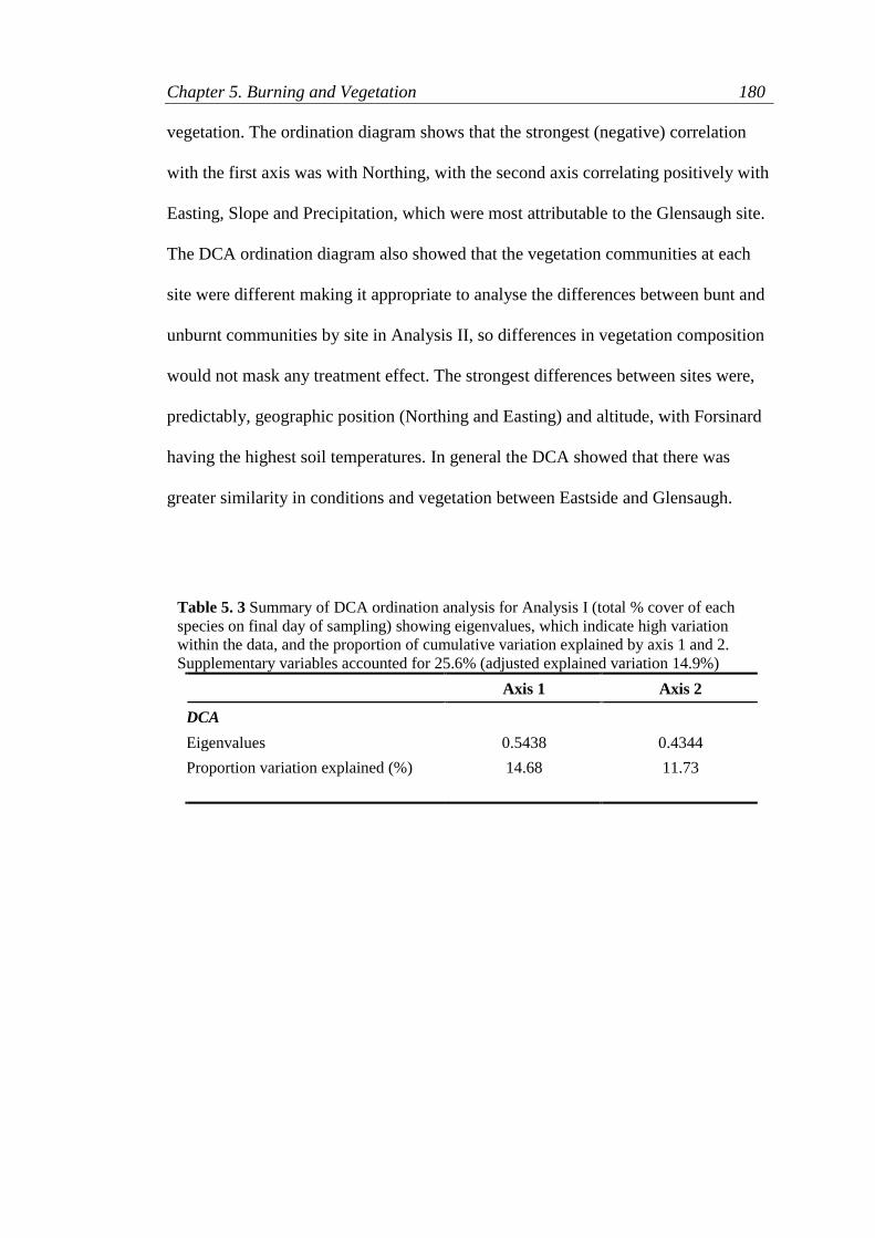
Chapter 5. Burning and Vegetation 180
vegetation. The ordination diagram shows that the strongest (negative) correlation
with the first axis was with Northing, with the second axis correlating positively with
Easting, Slope and Precipitation, which were most attributable to the Glensaugh site.
The DCA ordination diagram also showed that the vegetation communities at each
site were different making it appropriate to analyse the differences between bunt and
unburnt communities by site in Analysis II, so differences in vegetation composition
would not mask any treatment effect. The strongest differences between sites were,
predictably, geographic position (Northing and Easting) and altitude, with Forsinard
having the highest soil temperatures. In general the DCA showed that there was
greater similarity in conditions and vegetation between Eastside and Glensaugh.
Table 5. 3 Summary of DCA ordination analysis for Analysis I (total % cover of each
species on final day of sampling) showing eigenvalues, which indicate high variation
within the data, and the proportion of cumulative variation explained by axis 1 and 2.
Supplementary variables accounted for 25.6% (adjusted explained variation 14.9%)
Axis 1 Axis 2
DCA
Eigenvalues 0.5438 0.4344
Proportion variation explained (%) 14.68 11.73
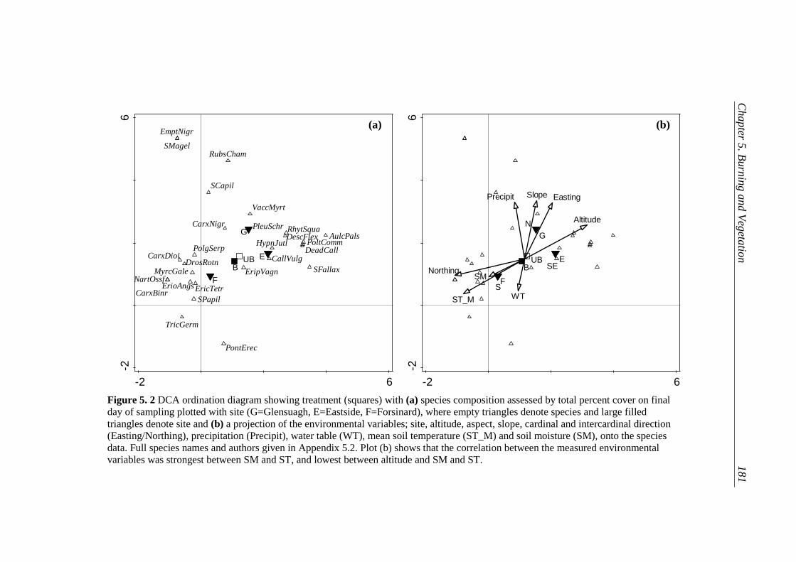
Figure 5. 2 DCA ordination diagram showing treatment (squares) with (a) species composition assessed by total percent cover on final
day of sampling plotted with site (G=Glensuagh, E=Eastside, F=Forsinard), where empty triangles denote species and large filled
triangles denote site and (b) a projection of the environmental variables; site, altitude, aspect, slope, cardinal and intercardinal direction
(Easting/Northing), precipitation (Precipit), water table (WT), mean soil temperature (ST_M) and soil moisture (SM), onto the species
data. Full species names and authors given in Appendix 5.2. Plot (b) shows that the correlation between the measured environmental
variables was strongest between SM and ST, and lowest between altitude and SM and ST.
-2 6
-26
BUB
G
E
F
AulcPals
CallVulgDeadCall
CarxBinr
CarxDioi
CarxNigr
DrosRotn
EmptNigr
EricTetrErioAngs
EripVagn
HypnJutl
MyrcGaleNartOssf
PleuSchr
PolgSerp
PontErec
RubsCham
SCapil
SMagel
SPapil
SFallax
TricGerm
VaccMyrt
DescFlexRhytSqua
PoltComm
-2 6
-26
SM
WTST_M
Altitude
Slope Easting
Northing
Precipit
BUB
N
SE
S
G
E
F
(a) (b)
Chapter 5
. Burn
ing a
nd V
egeta
tion
1
81

Chapter 5. Burning and Vegetation 182
5.5.1.2 Analysis II
To assess the differences between burnt and unburnt communities, and the
change in vegetation composition over time in the burnt plots, each site was assessed
separately using Principle Response Curves. All plots showed a one dimensional
direction of departure from the unburnt plots (vertical scores) with the greatest
difference in vegetation composition between burnt and unburnt plots found at T1
(Figure 5. 3 to 5.5). Common to all sites was a greater abundance of Eriophorum
vaginatum in the unburnt plots with the higher cover of litter (fragments of
unidentifiable plant material) in the burnt plots the most significant difference
between treatments at Eastside and Glensaugh.
At Forsinard (Figure 5. 3) there was greater cover of the Sphagnum mosses
S.capillifolium and S.papillosum as well as Eriophorum angustifolium and
Narthecium ossifragum in the burnt plots when compared to the unburnt plots. At
both Eastside and Glensaugh there was more dead Calluna in the burnt plots and in
general there were more dwarf shrubs in the unburnt plots at all sites: Erica tetralix
and Myrica gale at Forsinard and Glensaugh and Calluna vulgaris and Vaccinium
myrtillus at Eastside and Glensaugh. There was also greater cover of Rubus
chamaemorus in the burnt plots at Glensuagh, the only site at which it was found
(Figure 5. 5). Treatment was, however, only found to be significant at Eastside
(Table 5. 4) and that was the only site where there was a clear trend for the
vegetation composition of burnt plots becoming more like that of the unburnt
reference plots over the three sampling times (Figure 5. 4).

Chapter 5. Burning and Vegetation 183
In general, the percentage top cover of shrubs and graminoids was
consistently lower across the burnt plots than the unburnt plots with a strong trend
for graminoids increasing in the burnt plots over time (Figure 5. 6). Over the study
period however, graminoid cover in the burnt plots did not significantly exceed the
cover in the unburnt plots. There was not such a clear trend in shrubs, although shrub
cover in the burnt plots was consistently much lower than in unburnt plots at the first
sampling time. This remained the case at Eastside and Glensaugh at all sampling
times, however shrub cover was recorded as higher at time 2 in the burnt plots at
Forsinard. This is likely an artefact of the sampling method used as the shrubs at
Forsinard were smaller and lower growing, in contrast to the dominant shrub Calluna
at Glensaugh and Eastside, making them easily obscured by taller vegetation.
Table 5. 4 The amount of total and partial variance explained by Treatment and
Time for each site and the significance of Axis 1 (significant result shown in italics)
Site
Amount of Total
variation explained by
Time Treatment
Amount of Partial
Variance explained by
Treatment
Test on 1st
Axis
Forsinard 6% 20% 21.7% F=4.7
(p=0.15)
Eastside 23% 12% 15.9% F=5.5
(p=0.01)
Glensaugh 3% 5% 5.4% F=0.8
(p=0.54)

Chapter 5. Burning and Vegetation 184
Figure 5. 3 Principal Response Curve of Forsinard vegetation at the three sampling times
where burnt plots were compared to unburnt control plots and individual species scores (full
species names given in Appendix 5.2) for Axis 1 (a), (b). The effect of treatment and it’s
interaction with timepoint according to Monte Carlo permutation test was not significant
(p=0.148).
1.0 3.0PRC.Time
0.0
00.4
0P
RC
.1
Principal Response Curves
UB B
Species
-32
Resp.1
Litter
CallVulg
CarxBinr
CarxDioiDrosRotn
EricTetr
ErioAngs
EripVagn
HypnJutl
MyrcGale
NartOssf
PleuSchr
PolgSerp
PontErec
SCapil
SPapil
TricGerm
VaccMyrt
(a)
(a)
(b)

Chapter 5. Burning and Vegetation 185
Figure 5. 4 (a) Principal Response Curve of Eastside vegetation at the three sampling times
where burnt plots were compared to unburnt control plots and (b) individual species scores
(full species names given in Appendix 5.2).The effect of treatment and it’s interaction with
timepoint according to Monte Carlo permutation test was significant (p=0.01).
1.0 1.5 2.0 2.5 3.0
PRC.Time
0.0
0.1
0.2
0.3
0.4
0.5
PR
C.1
Principal Response Curves
UB B
Species
-3-2
-10
12
3
Resp.1
Litter
CallVulg
DeadCall
CarxNigr
DescCesp
ErioAngs
EripVagn
HypnJutl
JuncsSqu
PleuSchr
PontErec
SCapil
SFallax
VaccMyrt
RhytSqua
PlagUndl
(a)
(b)
(a)

Chapter 5. Burning and Vegetation 186
Figure 5. 5 (a) Principal Response Curve of Glensaugh vegetation at the three sampling
times where burnt plots were compared to unburnt control plots. The effect of treatment and
it’s interaction with timepoint according to Monte Carlo permutation test was not significant
(p=0.258) and (b) individual species scores. Full species names given in Appendix 5.2.
1.0 3.0PRC.Time
0.0
0.5
PR
C.1
Principal Response Curves
UB B
Species-2
.02.0
Resp.1
Litter
CallVulg
DeadCall
EmptNigr
EripVagn
PleuSchr
RubsCham
SCapil
VaccMyrt
(a)
(b)

Figure 5. 6 Difference in percentage cover of shrubs (a) and graminoids (b) at each site at each sampling time in the burnt and unburnt plots
(calculated as Burnt minus Unburnt percentage cover) where minus values represent a lower cover in the burnt plots when compared to
unburnt plots. The shrub group consisted Calluna vulgaris (dominant), Vaccinium myrtillus, Myrica gale and Erica tetralix. The graminoid
group was made up of Eriophorum vaginatum (dominant), Eriophorum angustifolium and Deschampsia flexuosa.
(a) (b)
Chapter 5
. Burn
ing a
nd V
egeta
tion
1
87

Chapter 5. Burning and Vegetation 188
5.5.1.3 NVC Classifications
All three sites were matched to different NVC sub communities with
classifications changing over time and occasionally, rather than consistently,
showing differences in NVC community between treatments (Table 5. 5,
Figure 5.7). Notably, NVC classifications were found to change over time in
both the unburnt plots and the burnt plots at all three sites. At some sampling times
there were relatively few species recorded, particularly in the burnt plots at Eastside
and at Glensaugh at the first sampling time, which meant matched sub-communities
were verified with the literature to ensure sensible matches.
Eastside was most often matched to M15b Scirpus cespitosus- Erica tetralix
wet heath however at sampling time 1 (T1) the unburnt plots were most closely
matched to M20b Eriophorum vaginatum mire: Calluna vulgaris- Cladonia sub
community. On the final day of sampling (T3) the burnt plots deviated from the
M15b classification, being more closely associated with M19b Calluna vulgaris –
Eriophorum vaginatum mire: Empetrum nigrum sub-community. This change in
community from M15 to M19 is likely due to the increase in graminoids cover in the
burnt plots, in particular an increase in E.vaginatum and Calluna with the lack of
Sphagnum spp. recorded in the burnt plots at T1 responsible for the M15/M20 split
between the burnt and unburnt communities.
The NVC classifications matched to the vegetation communities at Forsinard
varied from M17a Scirpus cespitosus – Eriophorum vaginatum blanket mire Drosera
– Sphagnum sub community to M15b Scirpus cespitosus – Erica tetralix wet heath
Chapter 5. Burning and Vegetation 189
typical sub community in both the burnt and unburnt plots. The burnt plots at
Forsinard were matched to the same communities as the unburnt plots at T2 and T3
while at T1 the best NVC match was M15c Scirpus cespitosus – Erica tetralix:
Cladonia sub community which could be a reflection of less Sphagnum being
detected in the burnt plots.
Table 5. 5 NVC sub communities matched to burnt and unburnt control
community at each site and sampling time (T1, T2, T3) showing the number of
species in each community and match statistics.
T1 T2 T3
B UB B UB B UB
Eastside
Number of spp. 3 5 8 11 8 12
Matched Community M15b M20b M15b M15b M19b M15b
Matching spp. 3/3 4/5 8/8 9/11 7/8 10/12
Weighted spp. match 100 100 100 91 90 92
Freq. Weighted match 86 94 75 74 68 73
Forsinard
Number of spp. 10 6 9 7 15 14
Matched Community M15c M17a M17a M17a M15b M15b
Matching spp. 10/10 6/6 9/9 7/7 15/15 13/14
Weighted spp. match 100 100 100 100 100 94
Freq. Weighted match 82 76 68 73 70 68
Glensaugh
Number of spp. 4 4 6 4 8 5
Matched Community M20b M20b M20b M20b M19a M20b
Matching spp. 4/4 4/4 6/6 4/4 8/8 5/5
Weighted spp. match 100 100 100 100 100 100
Freq. Weighted match 86 78 87 79 70 84
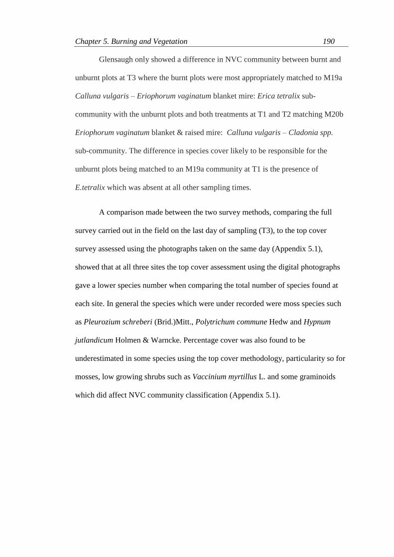
Chapter 5. Burning and Vegetation 190
Glensaugh only showed a difference in NVC community between burnt and
unburnt plots at T3 where the burnt plots were most appropriately matched to M19a
Calluna vulgaris – Eriophorum vaginatum blanket mire: Erica tetralix sub-
community with the unburnt plots and both treatments at T1 and T2 matching M20b
Eriophorum vaginatum blanket & raised mire: Calluna vulgaris – Cladonia spp.
sub-community. The difference in species cover likely to be responsible for the
unburnt plots being matched to an M19a community at T1 is the presence of
E.tetralix which was absent at all other sampling times.
A comparison made between the two survey methods, comparing the full
survey carried out in the field on the last day of sampling (T3), to the top cover
survey assessed using the photographs taken on the same day (Appendix 5.1),
showed that at all three sites the top cover assessment using the digital photographs
gave a lower species number when comparing the total number of species found at
each site. In general the species which were under recorded were moss species such
as Pleurozium schreberi (Brid.)Mitt., Polytrichum commune Hedw and Hypnum
jutlandicum Holmen & Warncke. Percentage cover was also found to be
underestimated in some species using the top cover methodology, particularity so for
mosses, low growing shrubs such as Vaccinium myrtillus L. and some graminoids
which did affect NVC community classification (Appendix 5.1).

42 198 479
Eastside M15b M15b M19b M20b M15b M15b
87 428 766
Forsinard M15c M17a M15b M17a M17a M15b
85 167 440
Glensaugh M20b M20b M19a M20b M20b M20b
Recovery Days
Figure 5.7 NVC sub-communities matched to the vegetation at each site over time and treatments using top cover survey method. Grey
boxes show the NVC community matched to the burnt treatment plots, white boxes the unburnt control plots. Consistent classifications are
outlined. Numbers in italics are recovery day (number of days since fire) on which the sites were surveyed. All sub-communities were ranked
#1 matches by the software apart from Glensaugh T3 where the burnt plots rank #1 match M18a was rejected as it is a community of lower
altitude and raised bogs and dominated by Sphagnum, and rank #2 M19c rejected due to the complete absence of Vaccinium vitis-idaea a
constant of this community. Rank #1 sub-community for the unburnt plots was M17c however this was rejected due to it being more
associated with lower altitudes in the west, which favoured rank #2 M20b which had the same match statistics.
Chapter 5
. Burn
ing a
nd V
egeta
tion 1
91
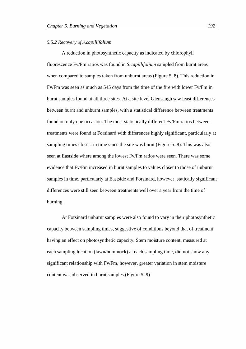
Chapter 5. Burning and Vegetation 192
5.5.2 Recovery of S.capillifolium
A reduction in photosynthetic capacity as indicated by chlorophyll
fluorescence Fv/Fm ratios was found in S.capillifolium sampled from burnt areas
when compared to samples taken from unburnt areas (Figure 5. 8). This reduction in
Fv/Fm was seen as much as 545 days from the time of the fire with lower Fv/Fm in
burnt samples found at all three sites. At a site level Glensaugh saw least differences
between burnt and unburnt samples, with a statistical difference between treatments
found on only one occasion. The most statistically different Fv/Fm ratios between
treatments were found at Forsinard with differences highly significant, particularly at
sampling times closest in time since the site was burnt (Figure 5. 8). This was also
seen at Eastside where among the lowest Fv/Fm ratios were seen. There was some
evidence that Fv/Fm increased in burnt samples to values closer to those of unburnt
samples in time, particularly at Eastside and Forsinard, however, statically significant
differences were still seen between treatments well over a year from the time of
burning.
At Forsinard unburnt samples were also found to vary in their photosynthetic
capacity between sampling times, suggestive of conditions beyond that of treatment
having an effect on photosynthetic capacity. Stem moisture content, measured at
each sampling location (lawn/hummock) at each sampling time, did not show any
significant relationship with Fv/Fm, however, greater variation in stem moisture
content was observed in burnt samples (Figure 5. 9).
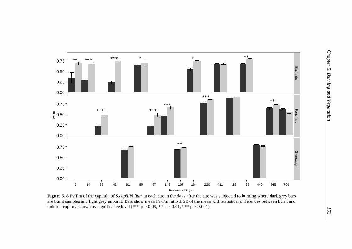
Figure 5. 8 Fv/Fm of the capitula of S.capillifolium at each site in the days after the site was subjected to burning where dark grey bars
are burnt samples and light grey unburnt. Bars show mean Fv/Fm ratio ± SE of the mean with statistical differences between burnt and
unburnt capitula shown by significance level (*** p=<0.05, ** p=<0.01, *** p=<0.001).
0.00
0.25
0.50
0.75
0.00
0.25
0.50
0.75
0.00
0.25
0.50
0.75
Easts
ide
Fors
inard
Gle
nsaugh
5 14 38 42 81 85 87 143 167 184 220 411 428 439 440 545 766
Recovery Days
Fv/F
m
Treatment
B
UB
*** **
***
*** *
*** ***
**
*
***
**
**
Chapter 5
. Burn
ing a
nd V
egeta
tion
1
93

Figure 5. 9 Stem moisture content of a sample of S.capillifolium removed from each hummock plotted with mean Fv/Fm (±StE bars) of the
capitula of and (b) mean (±StE bars) stem moisture content of burnt and unburnt samples at each site and sampling day where recovery day
was the number of says since sites were burned.
-0.5
0.0
0.5
1.0
80 85 90 95 100
Stem Moisture Content (% w et w eight basis)
Fv/F
m
Treatment
B
UB
60
70
80
90
5 14 38 42 81 85 87 143 167 220 428
Recovery DaysS
tem
Mois
ture
Conte
nt (%
wet w
eig
ht basis
)
Treatment
B
UB
Site
Eastside
Forsinard
Glensaugh
(b) (a)
Chapter 5
. Burn
ing a
nd V
egeta
tion
1
94

Chapter 5. Burning and Vegetation 195
As hypothesied, the photosynthetic capacity of S. capillifolium capitula was
related to new growth, with higher Fv/Fm measured on new capitula growing in the
burnt areas (Figure 5. 10). The new auxillay stems and capitula, which grew from the
old fire damaged stems, was observed at all three field sites (Figure 5. 11). At each
field site the hummocks and lawns of S. capillifolium where this new growth was
found appeared “speckled”, with new red (or green in some instaces) capitula a stark
contrast with the bleached old stem material, with no capitula, surrounding them
(Figure 5. 12). In some instance these areas of new growth were observed in
hummocks which were significantly damaged by the fire in parts, with extensive
bleaching and no apparent regrowth (Appendix 5.3).
Figure 5. 10 Mean (±StE bars) Fv/Fm of the capitula of S.capillifolium at Eastside which
had been burned 184 days previously (Burnt), compared to unburnt hummocks (Unburnt)
and new auxiliary capitula (New) found growing on stems in hummocks which had been
damaged by the fire (see Figure 5. 12). The results of a Kruskal–Wallis test were significant
(df=2, p=<0.001).
0.0
0.2
0.4
0.6
Burnt New Unburnt
Sample
Fv/F
m
Sample
Burnt
New
Unburnt

Chapter 5. Burning and Vegetation 196
Figure 5. 11 New auxiliary growth observed on S.capillifolium stems that had been
subjected to burning at Eastside (photograph taken 184 days after the fire had occurred).
The same auxiliary growth was seen at all three sites.
Figure 5. 12 A hummock of S.capillifolium at Forsinard which had been burnt 428 days
previously showing the new auxiliary growth which appear as red capitula surrounded by
bleached material (the remainder of the original stem) (enlarged in inset)

Chapter 5. Burning and Vegetation 197
5.6 Discussion
5.6.1 Changes in vegetation composition
There were distinct differences in vegetation composition between the three
sites studied, reflected by the different NVC sub-communities each site could be
most confidently assigned to. The sites most similar, both in terms of vegetation
composition and environmental conditions, were Eastside and Glensaugh. The most
species rich, in terms of species number, was Forsinard. Already this shows that
there were fundamental differences in pre-burn conditions even though the field sites
were established because they were similar, could be described as blanket bog with
peat deposits greater than 50cm, and were all burned by low severity fires. These site
level differences in vegetation composition and structure highlight the potential
variability in pre-burn conditions which may exist and shows how, even fires similar
in behaviour, could have different implications for vegetation. The results therefore
confirm the initial hypothesis [1], that there would be differences in species
composition between the three sites. Despite these differences however, as
hypothesised, there were common trends in composition change over time and
between treatments.
As would be expected by the visual observations of the fires, which removed
mostly just the canopy vegetation, both graminoids and shrubs were lower in the
burnt plots. Graminoid cover did, however, increase over time to levels seen in the
unburnt plots. Frequent burning is associated with the promotion of graminoids over
shrubs (eg. Stewart et al., 2004, Lee et al., 2013) but it is important to make the
distinction here, that graminoid cover could not be said to be increased by fire, rather
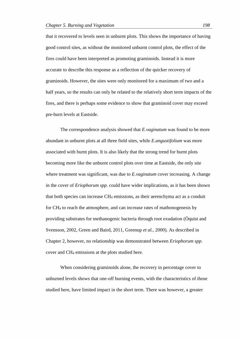
Chapter 5. Burning and Vegetation 198
that it recovered to levels seen in unburnt plots. This shows the importance of having
good control sites, as without the monitored unburnt control plots, the effect of the
fires could have been interpreted as promoting graminoids. Instead it is more
accurate to describe this response as a reflection of the quicker recovery of
graminoids. However, the sites were only monitored for a maximum of two and a
half years, so the results can only be related to the relatively short term impacts of the
fires, and there is perhaps some evidence to show that graminoid cover may exceed
pre-burn levels at Eastside.
The correspondence analysis showed that E.vaginatum was found to be more
abundant in unburnt plots at all three field sites, while E.angustifolium was more
associated with burnt plots. It is also likely that the strong trend for burnt plots
becoming more like the unburnt control plots over time at Eastside, the only site
where treatment was significant, was due to E.vaginatum cover increasing. A change
in the cover of Eriophorum spp. could have wider implications, as it has been shown
that both species can increase CH4 emissions, as their aerenchyma act as a conduit
for CH4 to reach the atmosphere, and can increase rates of mathonogenesis by
providing substrates for methanogenic bacteria through root exudation (Öquist and
Svensson, 2002, Green and Baird, 2011, Greenup et al., 2000). As described in
Chapter 2, however, no relationship was demonstrated between Eriophorum spp.
cover and CH4 emissions at the plots studied here.
When considering graminoids alone, the recovery in percentage cover to
unburned levels shows that one-off burning events, with the characteristics of those
studied here, have limited impact in the short term. There was however, a greater
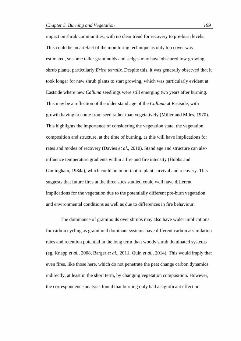
Chapter 5. Burning and Vegetation 199
impact on shrub communities, with no clear trend for recovery to pre-burn levels.
This could be an artefact of the monitoring technique as only top cover was
estimated, so some taller graminoids and sedges may have obscured low growing
shrub plants, particularly Erica tetralix. Despite this, it was generally observed that it
took longer for new shrub plants to start growing, which was particularly evident at
Eastside where new Calluna seedlings were still emerging two years after burning.
This may be a reflection of the older stand age of the Calluna at Eastside, with
growth having to come from seed rather than vegetatively (Miller and Miles, 1970).
This highlights the importance of considering the vegetation state, the vegetation
composition and structure, at the time of burning, as this will have implications for
rates and modes of recovery (Davies et al., 2010). Stand age and structure can also
influence temperature gradients within a fire and fire intensity (Hobbs and
Gimingham, 1984a), which could be important to plant survival and recovery. This
suggests that future fires at the three sites studied could well have different
implications for the vegetation due to the potentially different pre-burn vegetation
and environmental conditions as well as due to differences in fire behaviour.
The dominance of graminoids over shrubs may also have wider implications
for carbon cycling as graminoid dominant systems have different carbon assimilation
rates and retention potential in the long term than woody shrub dominated systems
(eg. Knapp et al., 2008, Barger et al., 2011, Quin et al., 2014). This would imply that
even fires, like those here, which do not penetrate the peat change carbon dynamics
indirectly, at least in the short term, by changing vegetation composition. However,
the correspondence analysis found that burning only had a significant effect on

Chapter 5. Burning and Vegetation 200
vegetation composition at Eastside, despite similar pre-burn vegetation composition,
structure and fuel loads to Glensaugh. This suggests that the fires behaved
differently, evident in the greater amount of Calluna biomass left by the fire at
Glensaugh indicating a fire lower in severity, and confirms that fire behaviour is also
important to consider. In addition, Eastside was surveyed closer to the time of fire,
when vegetation composition in burnt and unburnt plots was most different. Together
this highlights the dynamic impact of fires on vegetation, related to fire behaviour
and time since a fire. This would be important to build into any model of the impact
of fire on vegetation and carbon cycling in blanket bogs, and makes it necessary that
methods to assess the impact of a fire have the ability to relate to fire behaviour and
time since burning.
5.6.2 NVC Classifications
In respect to the hypothesis that the NVC system would offer a way of
reflecting differences in vegetation composition brought about by a fire, NVC
community matches were found to vary with site and treatment. However, they also
varied in both burnt and unburnt communities over time. The NVC communities
ascribed to each site and treatment did reflect the changes in dominant vegetation,
particularly the graminoids such as E.vaginatum, brought about by the fires.
However, the inconsistency in the NVC classifications given to the unburnt control
communities at two of the sites suggests that, to a degree it reflected seasonal
changes in dominant vegetation cover as well as the surveying procedures. There is
evidence of a seasonal effect on the NVC classifications as more vigorous growth
may have obscured mosses, often key to prescribing an NVC community. However,

Chapter 5. Burning and Vegetation 201
this will be an artefact of the surveying method as only top cover estimates were used
to assess change over time. This does highlight the importance of carrying out a full
assessment of cover, including the moss layer, to robustly assign an NVC
community. Despite only using top cover estimates, however, the results do indicate
both the capability and the limitations of using the NVC system to evaluate the
impact of fire on blanket bog vegetation.
The results show that the NVC communities assigned to Glensaugh were
most consistently the same between treatments and time points. This agrees with the
observation that this was the least severe fire. This suggests that the NVC system can
show, to some degree, the severity of the fire in terms of the degree of difference
between burnt and unburnt vegetation communities. Where it is limited however, is
in describing some of the changes in vegetation potentially important to the wider
functional condition and ecology of a blanket bog system. For example, structural
changes in vegetation cover are not described by NVC, so a shift in mature or
degenerate heather stands to pioneer seedling cover is not distinguished. This would
have particularly important implications for managed burning and rotation times as
for example, Calluna has different modes for re-growth depending on age and
structure, with post fire recovery shown to be slower in old Calluna stands (Hobbs
and Gimingham, 1984b, Davies et al., 2010). Plant biomass and structure have also
been related to fire behaviour (eg. Kayll, 1966, Hobbs and Gimingham, 1984a,
Molina and Llinares, 2001, Davies et al., 2010) which will be important to plant
survival and recovery. Post fire, the change in structure, particularly of canopy
species, may be important to low growing plants, such as the bryophytes which will

Chapter 5. Burning and Vegetation 202
have to be able to tolerate greater light exposure and potentially different moisture
conditions. This was shown here in an apparent increase in cover S. capillifolium in
burnt plots, but as the survey estimated top cover this only reflected the loss of the
canopy. In addition, the stem moisture content of S. capillifolium was shown to be
much more variable in the burnt plots, which may have implications for
photosynthesis (Schipperges and Rydin, 1998, van Gaalen et al., 2007, Strack et al.,
2009).
Over the timescale studied here some of the more subtle changes in species
cover were shown in the NVC matches, such as the presence of Rubus chamaemorus
only in the burnt plots, a species capable of dominating after fire due to spreading
rhizomes (Hobbs, 1984). However, using NVC to assess longer term changes in
vegetation composition, particularly if there are no control plots for comparison, does
not solely show the impacts of fire, rather it is a representation of the vegetation
community at a particular location and time point, where vegetation may be strongly
associated with environmental conditions and long term management. The
cumulative effect of management, climate and environmental conditions is difficult
to unravel and thus attributing change to one element of disturbance, such as fire, is
difficult using a vegetation classification system alone. This suggests that it is
preferable that other indicators of the ecological impact of a fire event are assessed
along with vegetation composition, such as extent of bare peat and percentage
consumption of the moss layer, which can be associated directly to burning.

Chapter 5. Burning and Vegetation 203
5.6.3 Sphagnum Survival and Recovery
It was hypothesised that the capitula, when not consumed, would show a long
term reduction in photosynthetic capacity. This was confirmed at all three sites as,
even after over a year from the time of the fire, the photosynthetic capacity of the
capitula was significantly lower in S.capillifolium in the bunt area. The site which
showed the least difference between treatments was Glensaugh, which again
indicates the lower severity of the fire. However, despite the observed reduction in
photosynthetic capacity, long term this may not be important due to the observed
propensity for rapid re-growth of new healthy auxiliary stem and capitula. The
results show that S.capillifolium has the ability to recover from low severity fires,
and that this can be common as it was observed at all three sites studied. It would
now be important to see if this response extends to other species and under what
conditions, both in terms of fire severity and behaviour, do plants lose this ability.
However, even in these light fires there was significant variation in the extent of
damage and bleaching, found even within the same hummock or lawn area. This
suggests that variation in fire behaviour at the micro-scale is significant for the
impact of a fire on the Sphagnum layer. This again highlights the potential for
significant variability in the impacts of fire on vegetation and wider ecology of
blanket bog, and suggests that fire behaviour at different spatial scales is critical.
5.7 Conclusions
Hypothesis [1] can be accepted as, despite differences in vegetation
communities between sites, there was a common trend of fire increasing the
abundance of the more competitive graminoid species, while reducing shrub cover in

Chapter 5. Burning and Vegetation 204
the short term. There was, however, no clear trend for shrubs to increase to cover
levels of unburnt areas over the time monitored. This supports previous observations
and also suggests that even fires which remove mostly only the canopy vegetation
and do not penetrate the peat, could indirectly affect rates of carbon assimilation and
retention in the short term. The change in vegetation composition brought about by
the fires was reflected to some degree by the NVC system, confirming hypothesis
[2]. However, NVC did not show more subtle changes in species cover over time,
and would not be sufficient for showing the effect on rare, low frequency, species. In
addition, it does not describe other impacts of fire which could have important
implications for the ecology of a blanket bog system, such as vegetation age and
structure or extent of damage to the Sphagnum layer or peat. Hypothesis [3] was also
confirmed, as the capitula of S.capillifolium which had been burned did have lower
photosynthetic capacity throughout the monitoring period. Despite this however,
S.capillifolium was shown to be fairly robust and able to recover from the fires
studied here by growing new healthy stem and capitula. More widely the results
show how the impact of a fire on the vegetation of a blanket bog is dependent on fire
behaviour as well as pre burn vegetation structure and composition.
Chapter 5. Burning and Vegetation 205
5.8 References
ALLEN, S. E. 1964. Chemical Aspects of Heather Burning. Journal of Applied
Ecology, 1, 347-367.
ASHTON, C., REIN, G., RIVERA, J. D., TORERO, J. L., LEGG, C., DAVIES, M.
& GRAY, A. 2007. Experiments and observations of peat smouldering fires.
International Meeting of Fire Effects on Soil Properties. Barcelona:
University of Edinburgh.
BALL, T., BLACK, A. R. & MACDONALD, A. M. 2012. 120 year records of
spring flows in the Pentland Hills, Midlothian: geological controls and
response to drought. British Hydrological Society Annual Symposium. .
Dundee.
BARGER, N. N., ARCHER, S. R., CAMPBELL, J. L., HUANG, C.-Y., MORTON,
J. A. & KNAPP, A. K. 2011. Woody plant proliferation in North American
drylands: A synthesis of impacts on ecosystem carbon balance. Journal of
Geophysical Research: Biogeosciences, 116, G00K07.
CENTRE FOR ECOLOGY AND HYDROLOGY. 2012. CEH Carbon Catchments:
Forsinard [Online]. Available:
http://www.ceh.ac.uk/sci_programmes/CarbonCatchmentsForsinard.htm
[Accessed 27/11/2012 2012].
DAVIES, G. M., SMITH, A. A., MACDONALD, A. J., BAKKER, J. D. & LEGG,
C. J. 2010. Fire intensity, fire severity and ecosystem response in heathlands:
factors affecting the regeneration of Calluna vulgaris. Journal of Applied
Ecology, 47, 356-365.
ELKINGTON, T., DAYTON, N., JACKSON, D. L. & STRACHAN, I. M. 2001.
National Vegetation Classification: Field guide to mires and heaths.
Peterborough: Joint Nature Conservation Committee.
GIMINGHAM, C. H. 1972. Ecology of heathlands, London, Chapman & Hall.
GRAY, A. 2006. The influence of managemnet on the vegetation and carbon fluxes
of blanket bog. Ph.D, The University of Edinburgh.
GREEN, S. & BAIRD, A. 2011. A mesocosm study of the role of the sedge
Eriophorum angustifolium in the efflux of methane—including that due to
episodic ebullition—from peatlands. Plant and Soil, 1-12.
GREENUP, A. L., BRADFORD, M. A., MCNAMARA, N. P., INESON, P. & LEE,
J. A. 2000. The role of Eriophorum vaginatum in CH4 flux from an
ombrotrophic peatland. Plant and Soil, 227, 265-272.
Chapter 5. Burning and Vegetation 206
HÁJEK, T. & BECKETT, R. P. 2008. Effect of Water Content Components on
Desiccation and Recovery in Sphagnum Mosses. Annals of Botany, 101, 165-
173.
HAMILTON, A. 2000. The characteristics and effects of management fire on
blanket-bog vegetation in north-west Scotland. Ph.D, The University of
Edinburgh.
HOBBS, R. J. 1984. Length of Burning Rotation and Community Composition in
High-Level Calluna-Eriophorum Bog in Northern England. Vegetatio, 57,
129-136.
HOBBS, R. J. & GIMINGHAM, C. H. 1984a. Studies on Fire in Scottish Heathland
Communities .1. Fire Characteristics. Journal of Ecology, 72, 223-240.
HOBBS, R. J. & GIMINGHAM, C. H. 1984b. Studies on Fire in Scottish Heathland
Communities .2. Post-Fire Vegetation Development. Journal of Ecology, 72,
585-610.
HOBBS, R. J., MALLIK, A. U. & GIMINGHAM, C. H. 1984. Studies on Fire in
Scottish Heathland Communities .3. Vital Attributes of the Species. Journal
of Ecology, 72, 963-976.
JOINT NATURE CONSERVATION COMMITTEE. 2006. Common Standards
Monitoring Guidance for Upland habitats. Available:
http://jncc.defra.gov.uk/pdf/CSM_Upland_Oct_06.pdf [Accessed 17th
September 2014].
KAYLL, A. J. 1966. Some Characteristics of Heath Fires in North-East Scotland.
Journal of Applied Ecology, 3, 29-40.
KNAPP, A. K., BRIGGS, J. M., COLLINS, S. L., ARCHER, S. R., BRET-HARTE,
M. S., EWERS, B. E., PETERS, D. P., YOUNG, D. R., SHAVER, G. R.,
PENDALL, E. & CLEARY, M. B. 2008. Shrub encroachment in North
American grasslands: shifts in growth form dominance rapidly alters control
of ecosystem carbon inputs. Global Change Biology, 14, 615-623.
LEE, H., ALDAY, J. G., ROSE, R. J., O'REILLY, J. & MARRS, R. H. 2013. Long-
term effects of rotational prescribed burning and low-intensity sheep grazing
on blanket-bog plant communities. Journal of Applied Ecology, 50, 625-635.
LEGG, C. 2008. ComKey. 2.0 ed.: Unpublished.
LEVY, P. E., BURDEN, A., COOPER, M. D. A., DINSMORE, K. J., DREWER, J.,
EVANS, C., FOWLER, D., GAIAWYN, J., GRAY, A., JONES, S. K.,
JONES, T., MCNAMARA, N. P., MILLS, R., OSTLE, N., SHEPPARD, L.
J., SKIBA, U., SOWERBY, A., WARD, S. E. & ZIELIŃSKI, P. 2012.
Chapter 5. Burning and Vegetation 207
Methane emissions from soils: synthesis and analysis of a large UK data set.
Global Change Biology, 18, 1657-1669.
LOVAT, L. 1911. Heather Burning In: LESLIE, A. S. E. (ed.) The Grouse in Health
and Disease. London: Smith, Elder & Co.
MALLIK, A. U. & GIMINGHAM, C. H. 1983. Regeneration of Heathland Plants
Following Burning. Vegetatio, 53, 45-58.
MALTBY, E., LEGG, C. J. & PROCTOR, M. C. F. 1990. The Ecology of Severe
Moorland Fire on the North York Moors: Effects of the 1976 Fires, and
Subsequent Surface and Vegetation Development. Journal of Ecology, 78,
490-518.
MANNINEN, S., WOODS, C., LEITH, I. D. & SHEPPARD, L. J. 2011.
Physiological and morphological effects of long-term ammonium or nitrate
deposition on the green and red (shade and open grown) Sphagnum
capillifolium. Environmental and Experimental Botany, 72, 140-148.
MILLER, G. R. & MILES, J. 1970. Regeneration of Heather (Calluna-Vulgaris (L)
Hull) at Different Ages and Seasons in North-East Scotland. Journal of
Applied Ecology, 7, 51-&.
MOLINA, M. J. & LLINARES, J. V. 2001. Temperature-time curves at the soil
surface in maquis summer fires. International Journal of Wildland Fire, 10,
45-52.
ÖQUIST, M. G. & SVENSSON, B. H. 2002. Vascular plants as regulators of
methane emissions from a subarctic mire ecosystem. J. Geophys. Res., 107,
4580.
QUIN, S. L. O., ARTZ, R. R. E., COUPAR, A. M., LITTLEWOOD, N. A. &
WOODIN, S. J. 2014. Restoration of upland heath from a graminoid- to a
Calluna vulgaris-dominated community provides a carbon benefit.
Agriculture Ecosystems & Environment, 185, 133-143.
R CORE TEAM. 2013. R: A language and environment for statistical computing
[Online]. Vienna, Austria. Available: http://www.R-project.org/ [Accessed
20/5/2013 2013].
RAWES, M. & HOBBS, R. 1979. Management of Semi-Natural Blanket Bog in the
Northern Pennines. Journal of Ecology, 67, 789-807.
RODWELL, J. S. 1991. British Plant Communities. II. Mires and Heaths.
Cambridge, UK: Cambridge University Press.
ROSS, S., ADAMSON, H. & MOON, A. 2003. Evaluating management techniques
for controlling Molinia caerulea and enhancing Calluna vulgaris on upland
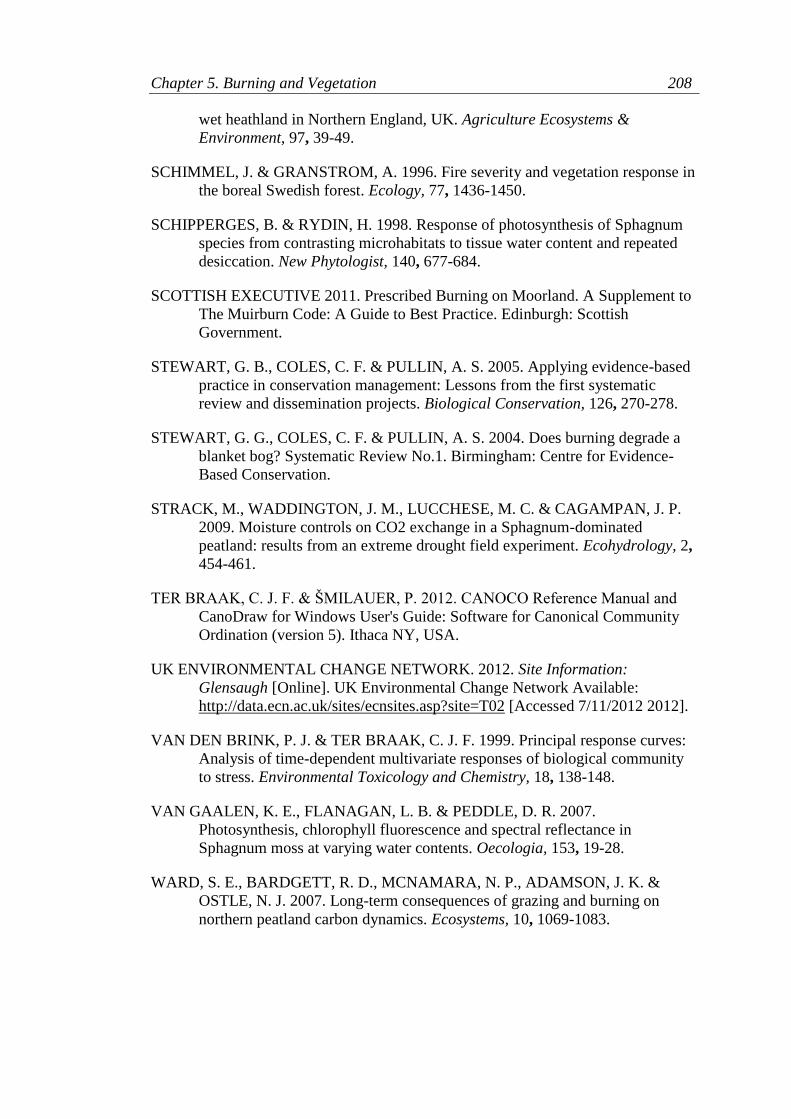
Chapter 5. Burning and Vegetation 208
wet heathland in Northern England, UK. Agriculture Ecosystems &
Environment, 97, 39-49.
SCHIMMEL, J. & GRANSTROM, A. 1996. Fire severity and vegetation response in
the boreal Swedish forest. Ecology, 77, 1436-1450.
SCHIPPERGES, B. & RYDIN, H. 1998. Response of photosynthesis of Sphagnum
species from contrasting microhabitats to tissue water content and repeated
desiccation. New Phytologist, 140, 677-684.
SCOTTISH EXECUTIVE 2011. Prescribed Burning on Moorland. A Supplement to
The Muirburn Code: A Guide to Best Practice. Edinburgh: Scottish
Government.
STEWART, G. B., COLES, C. F. & PULLIN, A. S. 2005. Applying evidence-based
practice in conservation management: Lessons from the first systematic
review and dissemination projects. Biological Conservation, 126, 270-278.
STEWART, G. G., COLES, C. F. & PULLIN, A. S. 2004. Does burning degrade a
blanket bog? Systematic Review No.1. Birmingham: Centre for Evidence-
Based Conservation.
STRACK, M., WADDINGTON, J. M., LUCCHESE, M. C. & CAGAMPAN, J. P.
2009. Moisture controls on CO2 exchange in a Sphagnum-dominated
peatland: results from an extreme drought field experiment. Ecohydrology, 2,
454-461.
TER BRAAK, C. J. F. & ŠMILAUER, P. 2012. CANOCO Reference Manual and
CanoDraw for Windows User's Guide: Software for Canonical Community
Ordination (version 5). Ithaca NY, USA.
UK ENVIRONMENTAL CHANGE NETWORK. 2012. Site Information:
Glensaugh [Online]. UK Environmental Change Network Available:
http://data.ecn.ac.uk/sites/ecnsites.asp?site=T02 [Accessed 7/11/2012 2012].
VAN DEN BRINK, P. J. & TER BRAAK, C. J. F. 1999. Principal response curves:
Analysis of time-dependent multivariate responses of biological community
to stress. Environmental Toxicology and Chemistry, 18, 138-148.
VAN GAALEN, K. E., FLANAGAN, L. B. & PEDDLE, D. R. 2007.
Photosynthesis, chlorophyll fluorescence and spectral reflectance in
Sphagnum moss at varying water contents. Oecologia, 153, 19-28.
WARD, S. E., BARDGETT, R. D., MCNAMARA, N. P., ADAMSON, J. K. &
OSTLE, N. J. 2007. Long-term consequences of grazing and burning on
northern peatland carbon dynamics. Ecosystems, 10, 1069-1083.
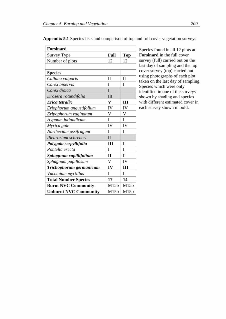
Chapter 5. Burning and Vegetation 209
Appendix 5.1 Species lists and comparison of top and full cover vegetation surveys
Forsinard
Survey Type Full Top
Number of plots 12 12
Species
Calluna vulgaris II II
Carex binervis I I
Carex dioica I
Drosera rotundifolia III
Erica tetralix V III
Eriophorum angustifolium IV IV
Eripophorum vaginatum V V
Hypnum jutlandicum I I
Myrica gale IV IV
Narthecium ossifragum I I
Pleurozium schreberi II
Polygala serpyllifolia III I
Pontella erecta I I
Sphagnum capillifolium II I
Sphagnum papillosum V IV
Trichophorum germanicum IV III
Vaccinium myrtillus I I
Total Number Species 17 14
Burnt NVC Community M15b M15b
Unburnt NVC Community M15b M15b
Species found in all 12 plots at
Forsinard in the full cover
survey (full) carried out on the
last day of sampling and the top
cover survey (top) carried out
using photographs of each plot
taken on the last day of sampling.
Species which were only
identified in one of the surveys
shown by shading and species
with different estimated cover in
each survey shown in bold.
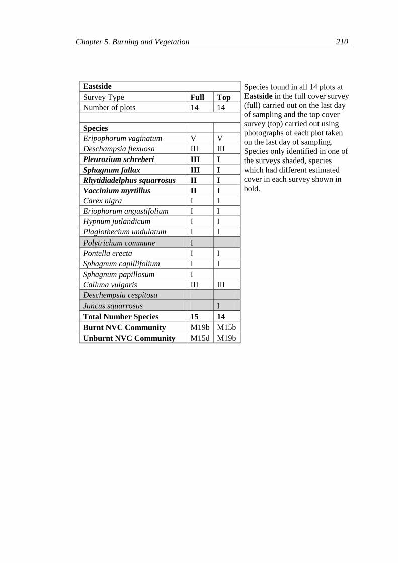
Chapter 5. Burning and Vegetation 210
Eastside
Survey Type Full Top
Number of plots 14 14
Species
Eripophorum vaginatum V V
Deschampsia flexuosa III III
Pleurozium schreberi III I
Sphagnum fallax III I
Rhytidiadelphus squarrosus II I
Vaccinium myrtillus II I
Carex nigra I I
Eriophorum angustifolium I I
Hypnum jutlandicum I I
Plagiothecium undulatum I I
Polytrichum commune I
Pontella erecta I I
Sphagnum capillifolium I I
Sphagnum papillosum I
Calluna vulgaris III III
Deschempsia cespitosa
Juncus squarrosus I
Total Number Species 15 14
Burnt NVC Community M19b M15b
Unburnt NVC Community M15d M19b
Species found in all 14 plots at
Eastside in the full cover survey
(full) carried out on the last day
of sampling and the top cover
survey (top) carried out using
photographs of each plot taken
on the last day of sampling.
Species only identified in one of
the surveys shaded, species
which had different estimated
cover in each survey shown in
bold.

Chapter 5. Burning and Vegetation 211
Glensaugh
Survey Type Full Top
Number of plots 8 8
Species
Aulacomnium palustre I
Calluna vulgaris II II
Empetrum nigrum I II
Erica tetralix II I
Eripophorum vaginatum IV V
Hypnum jutlandicum I
Pleurozium schreberi IV II
Rubus chamaemarus II I
Sphagnum capillifolium III III
Sphagnum magellanicum I
Vaccinium myrtillus IV IV
Total Number Species 11 8
Burnt NVC Community M18a M18a
Unburnt NVC Community M19c M17c
Species found in all 8 plots at
Glensaugh in the full cover
survey (full) carried out on the
last day of sampling and the top
cover survey (top) carried out
using photographs of each plot
taken on the last day of sampling.
Species only identified in one of
the surveys shaded, species
which had different estimated
cover in each survey shown in
bold.

Chapter 5. Burning and Vegetation 212
Appendix 5.2 Full species names and species author
Species name Abbreviation
Aulacomnium palustre (Hedw.) Schwägr. AulcPals
Calluna vulgaris (L.) Hull CallVulg
Dead Calluna DeadCall
Carex binervis Sm. CarxBinr
Carex dioica L. CarxDioi
Carex nigra (L.) Reichard CarxNigr
Drosera rotundifolia L. DrosRotn
Empetrum nigrum L. EmptNigr
Erica tetralix L. EricTetr
Eriophorum angustifolium Honk. ErioAngs
Eriophorum vaginatum L. EripVagn
Hypnum jutlandicum Holmen & Warncke HypnJutl
Myrica gale L. MyrcGale
Narthecium ossifragum Ker Gawl. NartOssf
Pleurozium schreberi (Brid.) Mitt. PleuSchr
Polygala serpyllifolia Hose. PolgSerp
Potentilla erecta (L.) Raeusch. PontErec
Rubus chamaemorus L. RubsCham
Sphagnum capillifolium (Ehrh.) Hedw. SCapil
Sphagnum magellanicum Brid. SMagel
Sphagnum papillosum Lindb. SPapil
Sphagnum fallax (Klinggr.) Klinggr. SFallax
Trichophorum germanicum Palla. TricGerm
Vaccinium myrtillus L. VaccMyrt
Deschampsia flexuosa (L.) Trin. DescFlex
Rhytidiadelphus squarrosus (Hedw.) Warnst. RhytSqua
Plagiothecium undulatum (Hedw.) Schimp. PlagUndl
Polytrichum commune Hedw. PoltComm
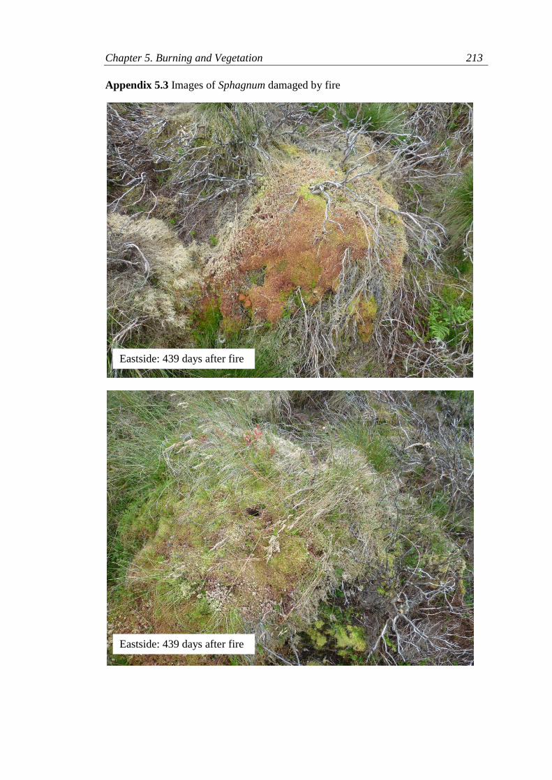
Chapter 5. Burning and Vegetation 213
Appendix 5.3 Images of Sphagnum damaged by fire
Eastside: 439 days after fire
Eastside: 439 days after fire

Chapter 5. Burning and Vegetation 214
Forsinard: 428 days after fire
Forsinard: 428 days after fire

Chapter 6. Synthesis 215
6. Synthesis
The aim of this research was to better understand some of the impacts of
burning on carbon cycling and the vegetation of blanket bogs. Through controlled
laboratory experiments and sampling at three fire sites over two and a half years, the
impacts of fire could be quantified and specific potential mechanisms for fire
modifying greenhouse gas emissions and damaging the Sphagnum layer could be
investigated. To address some of the gaps in our understanding of the impacts of
burning, important when prescribing best practice management, there were four
broad questions this research set out to answer:
1) Does fire increase methane emissions from blanket bogs? Is a reduction in
methanotrophy in the Sphagnum layer a potential mechanism for this?
2) Does ecosystem respiration change due to the changes in vegetation and
abiotic conditions after a fire that does not penetrate the peat?
3) How does Sphagnum respond to burning? Is there a critical temperature at
which Sphagnum cannot recover?
4) What short-term changes in blanket bog vegetation composition does fire
bring about? Do changes have wider implications for carbon cycling?
Despite these being distinct questions, and presented and discussed as such in each
chapter, the results need to be examined as a whole and considered in the context of
management guidance and policy. From this perspective the most important results

Chapter 6. Synthesis 216
relate to the effect low-severity fires have on greenhouse gas emissions, and the
critical factors for Sphagnum survival and recovery.
6.1 The impact of burning on greenhouse gas emissions from blanket bogs
Evaluating the impact of fire on blanket bogs, and whether it has a positive or
negative effect on their carbon budget, is increasingly relevant as more emphasis is
being placed on peatlands as carbon stores within the context of greenhouse gas
emissions from land use and land use change. This makes it necessary to revisit
management legislation and guidance to ensure it remains appropriate for this new
emphasis for good practice management. To do this, there has to be a sound evidence
base on which to amend the best practice guidelines. Historically in the UK
guidelines have been centred on the optimum management of heather, limiting the
risk of severe and dangerous fires, and potential damage to the wider environment
and wildlife. Therefore, this research set out to answer the specific questions of
whether fire increased CH4 emissions and ecosystem respiration from blanket bogs,
and if these increases were associated with changes in abiotic conditions, vegetation
composition and bacterial communities.
It was found that CH4 emissions were not significantly higher on burned
blanket bog when compared to adjacent areas that had not been burned. Likewise,
there was no trend for increased ecosystem respiration on the burned plots. This
suggests that the low severity fires studied (which did not penetrate the peat and left
the majority of the moss layer intact) did not increase carbon loss via these flux
pathways in the short (months) or medium term (less than 3 years). Both ecosystem

Chapter 6. Synthesis 217
respiration and CH4 emissions were found to be highly variable both within and
between sites and could not be related well to the vegetation composition of the plots
where fluxes were measured. There was a weak correlation between CH4 fluxes and
position of the water table and soil temperature, which is consistent with the
literature, but no differences were found in soil temperature, soil moisture and
position of the water table between the burned and unburned plots.
As the field study did not find any significant differences between burned and
unburned plots at any time, no short-term increase in methane emissions from the
burned plots was detected, as had been hypothesised. A mechanism that was
proposed for a potential short term increase in methane emissions from blanket bogs
after burning was a reduction in methanotrophy in the Sphagnum layer, caused by
high temperatures at the moss surface being lethal to methanotrophic bacteria. In the
laboratory experiment the only species of Sphagnum in which methanotrophy was
detected was Sphagnum papillosum Lindb., but no significant differences in CH4
oxidation rates of burned and unburned samples was detected. However, despite
testing various species from different micro-habitats the lack of methanotrophy
detected suggests that methanotrophic bacteria may not be as wide spread in
Sphagnum as previously reported. This would have broader implications for our
understanding of carbon cycling in blanket bogs, and it would be important to do
more widespread sampling of sites and species to better determine if the impact of
fire on methanotrophs has the potential to have any serious consequences for CH4
release from blanket bogs.

Chapter 6. Synthesis 218
In general the results indicate that low-severity fires, with the characteristics
of those studied here, do not significantly increase carbon loss via CH4 emissions and
CO2 emissions as a result of increased rates of ecosystem respiration. However, the
results should not be viewed in isolation, instead considered alongside the known
potential impacts of fire on the other carbon flux pathways not measured here.
Burning will directly increase carbon loss to the atmosphere through the
combustion of biomass, although the carbon lost in this way will only be that which
was sequestered by plants over relatively short timescales. More important therefore,
in terms of long term carbon storage, is carbon loss through the combustion of the
organic matter within the peat, formed over much longer timescales. There can be
significant carbon losses when fire penetrates the peat (eg. Turetsky and Wieder,
2001, Mack et al., 2011, Davies et al., 2013), and fire can change the structure and
functionality of a peatland in the long term (Maltby et al., 1990). Significantly, this
has been shown to be a mechanism for fire to turn peatlands from a net carbon sink
to a net source (Turetsky et al., 2011). As discussed fire may also have more subtle
interactions with components of the carbon cycle, such as changing the
methanotrophic community (Chen et al., 2008) or increasing decomposition through
the addition of nutrients in ash (Hogg et al., 1992). Carbon loss in run-off waters, in
the form of dissolved organic carbon (DOC), has also been shown to be higher after
a fire (Clay et al., 2009) and on blanket bog burned frequently as part of a
management regime (Yallop and Clutterbuck, 2009, Clutterbuck and Yallop, 2010).
As discussed in Chapter 5 frequent burning can also change vegetation composition,
which could lead to lower carbon sequestration rates (Garnett et al., 2000, Quin et
Chapter 6. Synthesis 219
al., 2014). At the sites studied here there was lower shrub and graminoid cover on
burned areas, although graminoid cover increased over the two and a half years
studied, so it is likely that carbon assimilation was affected at least in the short term
as a result of the fires. When considering all the potential impacts fire has been
shown to have on carbon cycling, it is important to appreciate the limitations of the
research and the results presented here. A major question, not directly answered by
this research, but pertinent to prescribing best practice guidance for managed
burning, is that of what are the most appropriate rotation times, the time period
between burns.
The consequences of repeated burning for the carbon cycle and vegetation of
a blanket bog will be the cumulative effect burning has on all carbon flux pathways,
most of which are inherently linked in some way to vegetation. Evident here was
that a single fire event brought about at least a short term change in vegetation
composition. Plants all have different traits in relation to lifecycle, growth, rates of
photosynthesis and decay with subsequent implications for carbon sequestration and
retention (eg. Belyea and Malmer, 2004, Quin et al., 2013, Quin et al., 2014). A
burning regime which favours one dominant vegetation type over another could
therefore have important implications for the long term carbon assimilation of a
blanket bog. In addition, different vegetation types have been associated with
different rates of DOC export (Limpens et al., 2008). Despite this however, there
may be reason to mitigate against severe fires with frequent, managed, low severity
fires to reduce fuel-load build up and the long-term risk of more severe fires. The
frequency and extent of the direct loss of carbon to the atmosphere via biomass

Chapter 6. Synthesis 220
combustion, and in severe fires the combustion of the peat, must be taken into
consideration when assessing the impact of different regimes on carbon budgets. In
addition, all the potential impacts of burning will be related in some way to the pre-
burn vegetation composition, plant survival, recovery and the viability of the existing
seed banks, and the behaviour of the fires. Therefore, not only will the optimum
burning rotation time, to reduce the likelihood of long term negative impacts on the
carbon cycle and carbon storage potential of a blanket bog, inevitably be site
specific, but it will have to strike a balance between these different potential impacts
of burning. This complexity makes it a challenge to model and predict the total
impact of different burning regimes, particularly when the vast majority of research
has occurred on frequently burned Calluna dominated systems. To better understand
the impact of different rotation times in different systems it is therefore essential to
monitor the consequences of different burning regimes in different blanket bog
vegetation communities as more refined, site specific, best practice guidelines are
likely needed. However, a key recommendation that can be made from the results
presented here, is that as low severity fires did not increase ecosystem respiration or
CH4 emissions from a blanket bog, it is important that burning does not take place in
circumstances which may allow for more severe fires which consume more than just
the canopy vegetation and penetrate the peat. This therefore makes it important that
any best practice burning guidance and legislation strives to mitigate the risk of more
severe fires, which could lead to significantly more short and long-term losses of
carbon.

Chapter 6. Synthesis 221
6.2 The Impacts of burning on Sphagnum
To better understand the impact of burning on the Sphagnum layer, how
Sphagnum responded to fire and whether there is a critical temperature at which
Sphagnum cannot recover was investigated. Lab based experiments and field
monitoring were carried out on Sphagnum capillifolium (Ehrh.) Hedw., chosen as it
is a species common to Calluna dominated blanket bog which can, in certain
circumstances, be burned as part of a moorland management regime (Scottish
Executive, 2011, Department for Environment Food and Rural Affairs, 2007).
The results of the laboratory experiment showed that the rate of recovery was
related to the temperature and temperature residency times experienced at the
Sphagnum surface. Samples exposed to 100oC for 3 seconds had the quickest
recovery, as indicated by photosynthetic capacity, while those which reached a
surface temperature of 400oC had slower rates of recovery and suffered more
physiological damage the longer the surface was at 400oC. The results also showed
that significant factors determining the rate of recovery and total damage sustained
were seasonality and pre burn stem moisture content. When samples were exposed to
the temperature treatments prior to cold winter months, recovery was slower which,
together with the very low rates of CO2 exchange found in unburned samples, reflect
a winter ‘dormancy’ period in S.capillifolium. Pre-burn conditions were also shown
to be important, with samples dried prior to burning, suffering a greater extent of
damage and decay. However, despite samples being artificially dried prior to being
exposed to the most severe heat treatment, 400oC for 30 seconds, designed to be
lethal, plants still showed signs of recovery. Thus, no critical lethal temperature
Chapter 6. Synthesis 222
treatment was demonstrated. However, taken with observations of some areas of
S.capillifolium at the field sites which showed no signs of recovery after
comparatively low-severity fires, it suggests that even these types of fires can be
lethal to Sphagnum. This may be because a combination of factors, beyond fire
behaviour and temperatures not simulated in the laboratory experiments, are
important. For instance, there was evidence here that stem moisture content was
more variable in burned S.capillifolium, which may make it less able to tolerate
desiccation. Trampling by grazing animals has also been shown to reverse recovery
of Sphagnum after burning (Hamilton, 2000). Nutrient input via ash deposition
(Niemeyer et al., 2005, Mohamed et al., 2007, Marcos et al., 2009) may also have
important consequences for Sphagnum survival. Nonetheless, the temperatures
experienced at the Sphagnum surface were shown to be directly related to how
S.capillifolium responded to the fires.
S.capillifolium, both at the three field sites and in the laboratory, was shown
to produce new auxiliary growth if the capitulum was damaged and lost. This
response was not identified in any lab samples which were exposed to the least
severe 100oC treatment in the laboratory experiment, where the capitulum remained
intact and recovered its photosynthetic capacity. This also suggests that the plants
monitored in the field had experienced temperature conditions exceeding those of the
least severe 100oC treatment simulated in the lab. This shows that even in low-
severity fires temperature conditions experienced at the Sphagnum surface in excess
of this are common. When new auxiliary stems were produced the location at which
they grew from the original stem related to the depth of decay from the capitulum
Chapter 6. Synthesis 223
down the stem. The depth of decay was related to the severity of the temperature
treatment with the most severe treatment, when stems were artificially dried,
showing the greatest depth of decay.
The depth of decay may be particularly critical for the ability of stems to
produce new auxiliary growth when the capitulum is lost. As Sphagnum grows from
the top of the stem while simultaneously decaying from the bottom, should
physiologically damaging temperatures penetrate down to the naturally decaying
lower sections, there may be not be the capacity for new growth from the original
stem if they are too physiologically degraded. There are also wider implications for
the deeper penetration of higher temperatures as it has been shown that, when
present, more methanotrophic bacteria can reside in these lower, decaying sections
(Basiliko et al., 2004, Raghoebarsing et al., 2005). Should temperatures exceed those
that are survivable by methanotrophic bacteria then this could be expected to have
implications on CH4 emissions from a bog. However, as discussed previously,
further investigation is needed as this was not confirmed by the experiments carried
out here.
Temperatures between 100oC and 400oC at the ground/bryophyte surface
have been shown to be common in Calluna dominated heath fires, but temperatures
remaining at 400oC and above for up to 30 seconds are less common (Davies, 2005).
Similar temperature ranges have been demonstrated in Calluna fires on blanket bog
but with a greater proportion of temperatures at the lower end of those recorded
(Hamilton, 2000). What is demonstrated here is that the temperatures and the
Chapter 6. Synthesis 224
temperature residency times at the ground/moss layer will be significant for
Sphagnum and are among the critical factors in determining the ability for the plants
to recover. Fuel load can be linked to the spatial variability in temperatures reached
at the ground surface in fires although high fuel loads may not necessarily increase
temperatures at the surface. This has been demonstrated in Calluna dominated heath
fires, where fires with low to medium fuel loads could experience the same ground
temperatures as high fuel load fires, associated with older stands of Calluna (Davies,
2005), suggesting that fuel structure is also important. The spatial variability in fuel
load and structure within and between fires (eg. Hobbs and Gimingham, 1984,
Davies, 2005, Davies et al., 2009) makes it difficult to quickly and effectively predict
the temperatures likely to be reached at the Sphagnum surface and thus their potential
impact on the Sphagnum layer. Therefore, low Sphagnum moisture content, another
critical factor in determining the impact on the Sphagnum demonstrated here, may be
a more useful field indicator of when not to carry out managed burning on blanket
bog if Sphagnum damage is to be limited.
Discussed thus far are the potential short term responses of one common
species of Sphagnum, but the affect of frequent burning on the Sphagnum layer and
the responses at a species level are also clearly important, particularly when
considering management regimes. Different Sphagnum species have been shown to
recover from fire at different rates (Barkman, 1992), which suggests that identifying
the key determinants for rates of recovery is complex beyond just the fire
characteristics, such as the temperatures experienced at the Sphagnum surface
studied here. As demonstrated, stem moisture content is likely to be critical in
Chapter 6. Synthesis 225
determining the extent of physiological damage and, as stem moisture content can be
related to morphology and growth habits, could make some species more tolerant to
burning than others. Dense, hummock forming species such as S.capillifolium, grow
in such a way to survive being further away from the water table, making them more
desiccation tolerant and better capable of retaining water (eg. Clymo, 1973, Luken,
1985). Interestingly, the field and lab evidence for new auxiliary growth to replace
lost capitula could mean that hummocks and lawns of S.capillifolium could become
denser, in terms of capitula number, as often the original stem would grow a number
of new auxiliary stems. However, these new auxiliary stems often appeared finer,
and not as robust as the original, which may have impactions for desiccation
tolerance and water retention in the long term. This would be an interesting avenue
for further research as not only could the differences in morphology mean some
species are more capable of surviving a fire, frequent burning may induce a change
in morphology in the long term which could either improve or reduce fire tolerance.
Another important factor which may be species specific is how tolerant a species is
to the post burn conditions, primarily the loss of the canopy vegetation. How well a
species recovers after burning is therefore related to a host of factors: pre burn
conditions such as stem moisture content, fire behaviour such as ground surface
temperatures, species morphology, and the post burn environmental conditions. This
makes the potential implication of a fire on the Sphagnum difficult to predict.
However, the results here would suggest that measures could be adopted to help limit
damage, the most obvious being not burning when the Sphagnum layer is particularly
dry.

Chapter 6. Synthesis 226
Although not studied here, but especially important when considering
management regimes and burning guidance, are burning frequency and rotation
times. Burning every 10 years compared to 20 years has been shown to have
different outcomes for the vegetation at the long term experimental burning site of
Hard Hill in the North Pennines (Gray, 2006, Rawes and Hobbs, 1979, Lee et al.,
2013), and a greater abundance of S.capillifolium has been found in the more
frequently burned plots (Lee et al., 2013). There is however, beyond the Hard Hill
experiment, little robust evidence of the effect of rotation times on Sphagnum and it
is clearly still vital for best practice management to research this further.
Another relevant aspect of the results, which may have implications for how
the severity of a fire can be assessed in the field, was the strong seasonal difference
in the rate of recovery. Delayed recovery due to winter dormancy means that in the
months after a fire the Sphagnum layer may seem more severely damaged because
there is no new growth and production of replacement capitula. This suggests that
October fires could seem to be more damaging than spring fires, purely due to the
rate of recovery and evidence of new growth being delayed until the spring months.
This makes using the damage caused to Sphagnum as an indicator of fire severity
potentially difficult, as in addition the response of losing capitula was delayed after
the time of burning. There is some evidence here however, that the loss of capitula
may indicate the temperatures experienced, with extensive capitula loss and a greater
depth of decay associated with higher surface temperatures and temperature
residency times.

Chapter 6. Synthesis 227
6.3 Conclusions and Implications for Management in the UK
What is demonstrated here is that to limit the detrimental effects of fire on
greenhouse gas emissions and the Sphagnum layer of blanket bogs, burning should
only take place in conditions which mitigate the risk of severe fires which burn more
than just the canopy vegetation. Critical to this will be moisture content of the
bryophyte layer, both to increase the chances of recovery in Sphagnum and to reduce
the risk of fire penetrating the deep into the Sphagnum layer and into peat. Currently
blanket bog in Scotland can be burned if heather constitutes more than 75% of the
vegetation (Scottish Executive, 2011) and in certain circumstances with agreed
management plans in England and Wales (Department for Environment Food and
Rural Affairs, 2007, Environment Agency Wales, 2008). To further mitigate the risk
of burning, when agreed and approved, on blanket bog where Sphagnum is an
important component of the vegetation, further provision should be made to ensure
conditions are conducive to low severity fires. This could include prescribing a basic
pre-burn assessment of the wetness/dryness of the moss layer and imposing
restrictions on burning in spells of prolonged dry weather. There will however be a
fine balance in achieving a burn on a blanket bog in the wet conditions necessary for
limiting damage, which may act to inherently reduce the occurrence of prescribed
burning on blanket bogs.
However, there is need for further research, particularly when considering the
effect of long term rotational burning on greenhouse gas emissions and vegetation, as
well as further investigation of the species level response of Sphagnum to fire. In
addition, this research supports the need to develop a system of categorising the
Chapter 6. Synthesis 228
ecological severity of a fire and their distribution and frequency at a national scale.
This is particularly important if burning is to be incorporated into national statistics
and frameworks for reporting green house gas emissions from land use and land use
change. Fire is ultimately a highly variable treatment, with both short term and long
term implications for vegetation and the carbon cycle of a blanket bog. Considering
the impact of fire on blanket bogs as one defined outcome, for example by assigning
it a standard emission factor, is therefore not appropriate and efforts have to be made
to understand the mechanisms behind the variability in effects. Only by
understanding the mechanisms which determine the severity of these effects, such as
the temperatures sustained at the moss surface or extent of peat consumption, can we
predict the outcome of fire on carbon cycling and vegetation and mitigate the risk of
detrimental fires through management guidance and legislation.

Chapter 6. Synthesis 229
6.4 References
BARKMAN, J. J. 1992. Plant communities and synecology of bogs and heath pools
in the Netherlands. In: VERHOEVEN, J. A. (ed.) Fens and Bogs in the
Netherlands. Dordrecht: Kluwer Academic Publishers.
BASILIKO, N., KNOWLES, R. & MOORE, T. 2004. Roles of moss species and
habitat in methane consumption potential in a northern peatland. Wetlands,
24, 178-185.
BELYEA, L. R. & MALMER, N. 2004. Carbon sequestration in peatland: patterns
and mechanisms of response to climate change. Global Change Biology, 10,
1043-1052.
CHEN, Y., DUMONT, M. G., MCNAMARA, N. P., CHAMBERLAIN, P. M.,
BODROSSY, L., STRALIS-PAVESE, N. & MURRELL, J. C. 2008.
Diversity of the active methanotrophic community in acidic peatlands as
assessed by mRNA and SIP-PLFA analyses. Environmental Microbiology,
10, 446-459.
CLAY, G. D., WORRALL, F. & FRASER, E. D. G. 2009. Effects of managed
burning upon dissolved organic carbon (DOC) in soil water and runoff water
following a managed burn of a UK blanket bog. Journal of Hydrology, 367,
41-51.
CLUTTERBUCK, B. & YALLOP, A. R. 2010. Land management as a factor
controlling dissolved organic carbon release from upland peat soils 2:
Changes in DOC productivity over four decades. Science of The Total
Environment, 408, 6179-6191.
CLYMO, R. S. 1973. Growth of Sphagnum - Some Effects of Environment. Journal
of Ecology, 61, 849-869.
DAVIES, G. M. 2005. Fire behaviour and impact on heather moorland. Ph.D,
University of Edinburgh.
DAVIES, G. M., GRAY, A., REIN, G. & LEGG, C. J. 2013. Peat consumption and
carbon loss due to smouldering wildfire in a temperate peatland. Forest
Ecology and Management, 308, 169-177.
DAVIES, G. M., LEGG, C. J., SMITH, A. A. & MACDONALD, A. J. 2009. Rate of
spread of fires in Calluna vulgaris-dominated moorlands. Journal of Applied
Ecology, 46, 1054-1063.

Chapter 6. Synthesis 230
DEPARTMENT FOR ENVIRONMENT FOOD AND RURAL AFFAIRS. 2007.
The Heather and Grass Burning Code [Online]. London: Department for
Environment, Food and Rural Affairs. Available:
http://www.naturalengland.org.uk/Images/heathergrassburningcode_tcm6-
7795.pdf.
ENVIRONMENT AGENCY WALES 2008. The Heather and Grass Burning Code
for Wales 2008. In: BRANCH, P. H. B. (ed.). Cardiff: Welsh Assembly
Government.
GARNETT, M. H., INESON, P. & STEVENSON, A. C. 2000. Effects of burning
and grazing on carbon sequestration in a Pennine blanket bog, UK. Holocene,
10, 729-736.
GRAY, A. 2006. The influence of managemnet on the vegetation and carbon fluxes
of blanket bog. Ph.D, The University of Edinburgh.
HAMILTON, A. 2000. The characteristics and effects of management fire on
blanket-bog vegetation in north-west Scotland. Ph.D, The University of
Edinburgh.
HOBBS, R. J. & GIMINGHAM, C. H. 1984. Studies on Fire in Scottish Heathland
Communities .1. Fire Characteristics. Journal of Ecology, 72, 223-240.
HOGG, E. H., LIEFFERS, V. J. & WEIN, R. W. 1992. Potential Carbon Losses
From Peat Profiles: Effects of Temperature, Drought Cycles, and Fire.
Ecological Applications, 2, 298-306.
LEE, H., ALDAY, J. G., ROSE, R. J., O'REILLY, J. & MARRS, R. H. 2013. Long-
term effects of rotational prescribed burning and low-intensity sheep grazing
on blanket-bog plant communities. Journal of Applied Ecology, 50, 625-635.
LIMPENS, J., BERENDSE, F., BLODAU, C., CANADELL, J. G., FREEMAN, C.,
HOLDEN, J., ROULET, N., RYDIN, H. & SCHAEPMAN-STRUB, G.
2008. Peatlands and the carbon cycle: from local processes to global
implications – a synthesis. Biogeosciences, 5, 1475-1491.
LUKEN, J. O. 1985. Zonation of Sphagnum Mosses: Interactions among Shoot
Growth, Growth Form, and Water Balance. The Bryologist, 88, 374-379.
MACK, M. C., BRET-HARTE, M. S., HOLLINGSWORTH, T. N., JANDT, R. R.,
SCHUUR, E. A. G., SHAVER, G. R. & VERBYLA, D. L. 2011. Carbon loss
from an unprecedented Arctic tundra wildfire. Nature, 475, 489-492.

Chapter 6. Synthesis 231
MALTBY, E., LEGG, C. J. & PROCTOR, M. C. F. 1990. The Ecology of Severe
Moorland Fire on the North York Moors: Effects of the 1976 Fires, and
Subsequent Surface and Vegetation Development. Journal of Ecology, 78,
490-518.
MARCOS, E., VILLALÓN, C., CALVO, L. & LUIS-CALABUIG, E. 2009. Short-
term effects of experimental burning on soil nutrients in the Cantabrian
heathlands. Ecological Engineering, 35, 820-828.
MOHAMED, A., HÄRDTLE, W., JIRJAHN, B., NIEMEYER, T. & GODDERT
VON, O. 2007. Effects of Prescribed Burning on Plant Available Nutrients in
Dry Heathland Ecosystems. Plant Ecology, 189, 279-289.
NIEMEYER, T., NIEMEYER, M., MOHAMED, A., FOTTNER, S. & HÄRDTLE,
W. 2005. Impact of prescribed burning on the nutrient balance of heathlands
with particular reference to nitrogen and phosphorus. Applied Vegetation
Science, 8, 183-192.
QUIN, S. L. O., ARTZ, R. R. E., COUPAR, A. M., LITTLEWOOD, N. A. &
WOODIN, S. J. 2014. Restoration of upland heath from a graminoid- to a
Calluna vulgaris-dominated community provides a carbon benefit.
Agriculture Ecosystems & Environment, 185, 133-143.
QUIN, S. L. O., CONOLLY, T. R. A., ARTZ, R. R. E., COUPAR, A. & WOODIN,
S. J. 2013. The Assimilation and Retention of Carbon in Upland Heath Plant
Communities Typical of Contrasting Management Regimes: A 13C Tracer
Study. Journal of Ecosystems, 2013, 10.
RAGHOEBARSING, A. A., SMOLDERS, A. J. P., SCHMID, M. C., RIJPSTRA,
W. I. C., WOLTERS-ARTS, M., DERKSEN, J., JETTEN, M. S. M.,
SCHOUTEN, S., SINNINGHE DAMSTE, J. S., LAMERS, L. P. M.,
ROELOFS, J. G. M., OP DEN CAMP, H. J. M. & STROUS, M. 2005.
Methanotrophic symbionts provide carbon for photosynthesis in peat bogs.
Nature, 436, 1153-1156.
RAWES, M. & HOBBS, R. 1979. Management of Semi-Natural Blanket Bog in the
Northern Pennines. Journal of Ecology, 67, 789-807.
SCOTTISH EXECUTIVE 2011. The Muirburn Code. Edinburgh: Scottish
Government.
TURETSKY, M. R., KANE, E. S., HARDEN, J. W., OTTMAR, R. D., MANIES, K.
L., HOY, E. & KASISCHKE, E. S. 2011. Recent acceleration of biomass

Chapter 6. Synthesis 232
burning and carbon losses in Alaskan forests and peatlands. Nature Geosci, 4,
27-31.
TURETSKY, M. R. & WIEDER, R. K. 2001. A direct approach to quantifying
organic matter lost as a result of peatland wildfire. Canadian Journal of
Forest Research, 31, 363-366.
YALLOP, A. R. & CLUTTERBUCK, B. 2009. Land management as a factor
controlling dissolved organic carbon release from upland peat soils 1: Spatial
variation in DOC productivity. Science of the Total Environment, 407, 3803-
3813.