NBER WORKING PAPER SERIES

THE IMPACT OF EMERGING CLIMATE RISKS ON URBAN REAL ESTATE PRICEDYNAMICS

Devin BuntenMatthew E. Kahn

Working Paper 20018http://www.nber.org/papers/w20018

NATIONAL BUREAU OF ECONOMIC RESEARCH1050 Massachusetts Avenue

Cambridge, MA 02138March 2014

We thank the Ziman Center for Real Estate at UCLA for generous funding. We would like to thankNicolai Kuminoff and Jaren Pope for helpful comments. This research was supported by Award NumberT32AG033533 from the National Institute on Aging. The content is solely the responsibility of theauthors and does not necessarily represent the official views of the National Institute on Aging or theNational Institutes of Health The views expressed herein are those of the authors and do not necessarilyreflect the views of the National Bureau of Economic Research.

NBER working papers are circulated for discussion and comment purposes. They have not been peer-reviewed or been subject to the review by the NBER Board of Directors that accompanies officialNBER publications.

© 2014 by Devin Bunten and Matthew E. Kahn. All rights reserved. Short sections of text, not to exceedtwo paragraphs, may be quoted without explicit permission provided that full credit, including © notice,is given to the source.

The Impact of Emerging Climate Risks on Urban Real Estate Price DynamicsDevin Bunten and Matthew E. KahnNBER Working Paper No. 20018March 2014JEL No. Q54,R3

ABSTRACT

In the typical asset market, an asset featuring uninsurable idiosyncratic risk must offer a higher rateof return to compensate risk-averse investors. A home offers a standard asset's risk and returnopportunities, but it also bundles access to its city's amenities|and to its climate risks. As climatechange research reveals the true nature of these risks, how does the equilibrium real estate pricinggradient change when households can sort into different cities? When the population is homogeneous,the real estate pricing gradient instantly reflects the "new news". With population heterogeneity, anevent study research design will underestimate the valuation of climate risk for households in low-risk cities while overestimating the valuation of households in high-risk areas.

Devin BuntenUniversity of California at Los AngelesDepartment of Economics8283 Bunche HallLos Angeles, CA 90095-1477devinbunten@gmail.com

Matthew E. KahnUCLA Institute of the EnvironmentDepartment of EconomicsDepartment of Public PolicyAnderson School of ManagementUCLA Law School, Box 951496Los Angeles, CA 90095-1496and NBERmkahn@ioe.ucla.edu

1 Introduction

In the absence of a global agreement on reducing world greenhouse gas emissions,climate change risk continues to be exacerbated by ongoing population and per-capita income growth. Rising greenhouse gas production increases atmosphericconcentrations of carbon dioxide and this increases the probability of extremeclimate events. Researchers working at the intersection of macro and environ-mental economics have evaluated the ex-ante social costs of “fat tail” disasterevents (Barro, 2013; Costello et al., 2010; Pindyck, 2013; Pindyck and Wang,2013; Weitzman, 2009, 2011). Macro models of climate changes consequenceshave often implicitly assumed away any spatial adaptation possibilities.1

Recent research on climate change adaptation has studied how changing climateconditions affects regional comparative advantage (Desmet and Rossi-Hansberg,2013; Costinot et al., 2012). The former present a general equilibrium modelfeaturing free trade across regions and study the welfare consequences of climatechange when the location of both production and households can shift as climateconditions shifts while the latter analyze the likely macro effects of micro-scalereallocations of cropland in the face of a changing climate.

Empirical studies have estimated cross-city real estate hedonic pricing regres-sions to predict how climate change is likely to impact the value of real estatein different locations (Albouy et al., 2013; Kahn, 2009). Intuitively, in the year2050 will the current real estate price differential between San Francisco and De-troit narrow if Detroit’s climate is predicted to improve (i.e. warmer winters)relative to San Francisco?

In this paper, we analyze the spatial implications of emerging climate risk withina system of cities, each of which may face different risks. Within a nation such asthe United States or a trading bloc such as the European Union, both labor andcapital can move to any location. This potential for spatial arbitrage imposescross-restrictions across real estate prices and local wages across space. In spatialequilibrium, both heterogeneous households and firms cannot raise their utilityand profits by moving to another location. Cross-city real estate prices andwages adjust to support such that the local land market and the local labormarket clear (Rosen, 2002).

We introduce a system of cities model to consider the economic incidence of anemerging new catastrophic risk (i.e., climate change). Throughout this paper,we assume that a known subset of cities face the most severe risk due to their

1Early work introducing a multi-region economy such as the Nordhaus and Yang (1996)RICE model did not allow for migration of labor across borders. In their model, regions differwith respect to their sectoral shares (i.e some regions have an agricultural focus while othersspecialize in manufacturing). They assume that the damage function from climate change isidentical for each industry across different regions, and then conduct a shift-share calculationto determine how a region is affected by climate change. For example, if a region’s economyspecializes in agriculture and if climate change impacts agriculture then this region will besharply impacted by climate change.

2

coastal geography. As climate scientists make progress and reveal the “newnews” that cities such as Miami, New Orleans and New York City face increasedrisk of large-scale disasters, we seek to understand how equilibrium real estateprices across cities evolve. We embed the future risk of climate change into aclassic Rosen/Roback (Rosen, 1979; Roback, 1982; Rosen, 2002) compensatingdifferentials model. Climate change risk is a tied local public bad that (inexpected value) poses future costs.

We contrast two main cases. In the first case, the population has homogenouspreferences over coastal amenity attributes, climate, and avoiding low proba-bility risks. The hedonic pricing gradient for homes immediately reflects the“new news” of the increased risk that cities such as Miami face due to risinggreenhouse gas emissions.

In the second case, we introduce population heterogeneity along several dimen-sions. The population can differ with respect to income, tastes for amenities,the ability to engage in self protection against emerging risks (see Ehrlich andBecker, 1972), and location-specific networks and knowledge. Together thesefactors create a wedge between the willingness to pay among coastal incumbenthome owners to remain in risky places versus the willingness to pay of outsidersconsidering moving to at risk cities. In this case, home prices in affected citiesmay not decline when the “new news” about climate risk becomes commonknowledge. This result can be derived even when everyone agrees about theserious risk that the coastal cities face. An econometrician conducting an eventstudy is likely to underestimate the average person’s willingness to pay to avoidclimate risk.

The key intuition here is to recognize that the marginal household, whose will-ingness to pay to live in the risky city sets the market price, may have a com-parative advantage in coping with local risk or may have built up city specificcapital (both social capital and local knowledge) such that this household effec-tively faces a higher migration cost for leaving the city. As we discuss below, thisendogenous differential valuation of the same city by “insiders” and “outsiders”has implications for considering the merits of place based disaster insurancesuch as government FEMA programs.

In the literature on the fat tails of rare disasters, households within the modelare aware of risks of which the econometrician is ignorant. In our model, thesituation is different: both households and the econometrician are fully awareof the objective risks facing different cities. In this paper, the econometricianis unaware of the type and degree of household heterogeneity. This limits theextent to which prices of real estate—determined by marginal agents—reflect thewillingness to pay of the average household. This limitation, due to residentialsorting based on observed and unobserved attributes of both the city and themigrant, bears a similarity to the work of Shogren and Crocker (1991) on theattributes incorporated into hedonic pricing functions. Our findings concerningthe information embedded in the hedonic gradient build on recent work byKuminoff and Pope (forthcoming) in studying the economic incidence of changes

3

in local public goods (in this case coastal safety).

Our findings build on past work in local public finance by scholars such as Star-rett (1981), who examined the conditions under which local public goods willbe capitalized completely, partially, or not at all. In that context, Lind (1973)and Kanemoto (1988) provide guidance on the interpretation of capitalizationstudies as providing bounds on the heterogeneous population’s willingness topay for location specific attributes.

In the last section of the paper, we discuss how essential heterogeneity (seeHeckman et al., 2006) affects inferences from standard hedonic real estate eventstudies where the event in question is the realization that specific cities facesevere climate change risk. Our findings have a similar flavor as the Shogren andStamland (2002, 2005) analysis of hedonic wage regressions seeking to recoverstatistical value of life estimates in the presence of essential heterogeneity.

2 Will Miami Vanish?

The motivating example for this paper is Miami. The Miami metropolitan areais home to six million people. The city itself is located six feet above sea level.In summer 2013, Rolling Stone magazine published a long front page articlefocusing on the claim that Miami is doomed because of imminent sea level rise(Goodell, 2013). This salient case study highlights the coming challenge thatthe U.S coastal population faces. Rappaport and Sachs (2003) document that amajority of the nation’s population and income is located in coastal and GreatLakes areas. In the case of Miami, urban planning documents highlight thatMiami-Dade County is planning for sea level rise (Miami-Dade County, 2010).The housing crisis notwithstanding, Miami home prices have increased nearlyas rapidly as those of far-inland Denver over the last thirty years, showing nostark decline as climate research has progressed.2

The apparent non-responsiveness of Miami real estate to changing climate riskposes a puzzle: why aren’t holders of Miami real estate assets compensatedfor this risk with a price discount? This puzzle is almost the inverse of theequity premium puzzle, where risk-averse investors hold bonds despite the lowreturns. The answer of Barro (2006) is that the fat-tails of consumption disas-ters, unobserved to the econometrician, lead investors to hold safer assets. Inour puzzle, people pay apparently large sums to hold risky assets—Miami realestate—whose risk profile has increased with the advent of climate change. Inour case, unobserved household heterogeneity means that only the householdsmost willing or capable of dealing with these risks choose to hold Miami realestate, limiting the price impacts of emerging climate risks.

2See Figure 1 in the appendix. Data from Trulia indicates that Miami coastal areas suchas Coral Gables and Miami Beach experienced an even more pronounced recent boom.

4

In considering the Miami case as a leading motivating example, we seek to focusattention to the damage natural disasters pose to the place-based capital stockrather than to human longevity. Cross-country research has documented thatnatural disasters are killing fewer people over time and that richer nations sufferfewer deaths from natural disasters (Kahn, 2005). We recognize that extremenatural disasters such as Hurricane Katrina which is estimated to have killedroughly 1,850 people in 2005 can be deadly. Valuing each life lost at $6 millionyields a total value of life lost at $11.1 billion. Estimates for the propertydamage from Hurricane Katrina are in the range of $100 billion (Knabb et al.,2005). An alternative way to look at the damage caused by Katrina is to recallthat in the year 2000 that New Orleans had a population of 490,000. Thismeans that the 1,850 deaths from Katrina represented 0.0038 of the area’s totalpopulation; for comparison there were 210 homicides in New Orleans in thesame year (Van Landingham, 2007).

In the case of Hurricane Sandy in 2012, this storm caused 117 deaths and atotal of $65 billion dollars of damage (Mulvihill, 2013; Newman, 2012). Thisexample highlights that the damage risk to physical property swamps the totaldeath risk. We believe that the ratio of total value of lives lost to climate changedisasters divided by the total damage to physical capital will only decline overtime. With the rise of smart phones and emergency warnings, we predict thatthe footloose coastal population (facing mandatory evacuations) will becomemore responsive to disaster alerts so that fewer people die in disaster eventswhile buildings and infrastructure are highly immobile and subject to extremedamage. This discussion motivates some of the modeling assumptions we makebelow.

3 A Model of Rare Disasters with Variable RiskAcross Cities

3.1 The Model with Homogeneous Households

Consider a model of household location choice where households maximize life-time utility. To choose a location j(t) ∈ J requires ownership of an asset hj(i.e., a home) that provides access to city j’s amenity aj and also its idiosyn-cratic maintenance shocks. The first maintenance shock is a small but regulardepreciation shock δj and the second is a rare but large catastrophic shock κj .

3

Both are i.i.d. across time, and independent across space.4

3In addition to housing capital, public capital is also at risk, and κj can be interpreted asincluding the risk that local homeowners will be compelled to rebuild damaged public capital.We discuss private capital in a later section.

4The same climatic pressures may create drought in one area and flooding in another, and ahurricane may impact multiple locales; the i.i.d assumption is a simplification. However, giventhat households choose one city at a time and they choose this city prior to the observation

5

Households are free to buy and sell these assets each period, and transactionsoccur prior to the realization of any shocks. For a household currently livingin city i who chooses to live in city j, lifetime utility is the discounted sumof period utilities, given by u(cij , aj). The houshold faces a period-by-periodbudget constraint of the form cij + (pj − δj − κj)hj = y + pihi where y is thehousehold endowment and pi is the equilibrium price in city i. The subscript ijdenotes a household that begins in city i and chooses to live in city j, recognizingthat consumption may be different for two households who both move to j butwho began in different cities.

For each city, there is a fixed supply of homes. This assumption can be inter-preted as each city having a fixed quantity of land that must be combined withhousing materials in a fixed proportion in order to produce housing services, andthat the depreciation and catastrophic shocks represent regular maintenance anddisaster-rebuilding, respectively. Alternatively, the assets can be interpreted astrees that bear two kinds of fruit: a fixed aj and a variable y − δjt − κjt. Seenin this light, the model is similar to those of Barro (2006, 2013), where we haveallowed for a variety of asset trees from which households must choose just one.

In equilibrium, households will not choose to move; they will have already sortedinto the city that maximizes their utility given relative prices. By assumption,each period’s location decisions are made before the shocks are observed andthus relative prices are invariant from period to period and depend only onexpected shocks.

We now consider the following asset pricing exercise to calculate the willingnessto pay for real estate in different cities. If a household residing in city i purchasesa home in city j for price pij , they expect to receive utility Uij = E[u(y+ (pi −pij)− δj − κj , aj)] +

∑∞t=1 β

tE[u(y − δjt − κjt, aj)]. By setting Uij = Ui, whereUi is the utility the household would receive if they stay, we can solve for themaximum price pij that the household would pay to move to city j.

(1)

E[u(y + (pi − pij)− δj − κj , aj)] +

∞∑t=1

βtE[u(y − δjt − κjt, aj)]

=∞∑t=0

βtE[u(y − δit − κit, ai)]

In the initial scenario, the κ and δ processes are stationary, and the equationcan thus be simplified.

(2)(1− β)E[u(y + (pi − pij)− δj − κj , aj)] + βE[u(y − δjt − κjt, aj)]

=E[u(y − δit − κit, ai)]

of shocks, their concern is with the average expected shock in their choice city, rather thanpossible correlations across cities.

6

We suppose that at some initial date zero, households were free to choose lo-cations and prices adjusted to make them indifferent. Those households whoinitially chose high-amenity and low-risk areas would have bid more initiallyand those high prices would persist in the steady state.

3.2 The Model with Heterogeneous Households

A similar equation can be derived in the case of heterogeneous households.While the potential types of household heterogeneity are limitless, we focus onthree key cases: variable income levels, variable self-protection abilities, and theformation of local endogeneous social networks.5 The first takes the form ofa different endowment yh, where h indexes households; the second involves autility parameter ρh that reduces the effects of the catastrophic shock κ; andthe third is modeled as a fixed moving cost µ. Solving the budget constraint forc and substituting again gives an equation that can be solved for the willingnessto pay of household h in city i considering a move to city j.

(3)(1− β)E[u(yh + (pi − pij)− δj − (1− ρh)κj , aj)]+

βE[u(yh − δjt − (1− ρ)κjt, aj)]− (1− β)µ = E[u(yh − δit − (1− ρ)κit, ai)]

We can use this equation to solve for initial distribution of households acrosscities. We further assume that the distributions of E[δi], E[κi], and ai aresuch that a priori, all residents agree on which is the“worst” city, which wedenote city l. Note that in equilibrium, pl = 0. Consider then Equation (3) forhousehold h in city l considering a move to city j. To solve for the distributionof households, consider each city j ∈ J and calculate the willingness to pay pljfor each household. Ordering these bids from highest to lowest, and recallingthat each city has a fixed supply of homes, call p̂j the willingness to pay of themarginal household. Take the city with the highest p̂j , and allocate to that citythose households willing to pay at least p̂j . After allocating these households,repeat the process for the remaining households and cities until all householdsare allocated. This is the initial equilibrium distribution of households. Notealso that the order in which the cities are selected offers an implicit ranking ofthe quality of life in these cities.

We use this distribution to solve for the set of prices across all cities. Beginningwith the last two cities allocated. Because the worst city l has pl = 0, the priceof the next-to-worst city is the price that makes the marginal household in cityl just indifferent between choosing the next city. Repeat this process for eachcity, moving up the implicit ranking identified previously. The last city priced

5The third case is reminiscent of Krupka (2009), where each household invests in humancapital that enhances its particular local amenities.

7

will be the first city that households were allocated to: that with the highestmarginal willingness to pay.6

After allocating households and solving for each city’s prices, the resultant equi-librium will initially be stable: the relative values of the various shocks are stableacross cities, and no household will be willing to pay to move a better city norinterested in paying less for less amenable city. This finding will not, in general,hold true in the next section after introducing climate change.

4 Climate Change Risk as “New News”

We now introduce climate change. Climate change is a one-time unanticipatedevent that alters the future risks of different cities in the economy. There isno learning per se: agents simply wake up to a new probability distribution offuture outcomes. As an example, they may discover that climate change willaffect Miami in the year 2040, Chicago in 2060, and Denver in 2080. They willalso uncover the magnitude of the effect in each city. In particular, householdslearn that the distribution of catastrophic shocks κi,t will worsen in the futurefor each city, as a function of the stock of global greenhouse gases. For eachcity, we suppose that there is a threshold level of greenhouse gases φi that willtrigger the one-time transition from relatively-low to relatively-high risk, wherethe relative changes may vary by city. If greenhouse gases rise predictably, thenthis translates to a threshold year which we call τi at which point city i willincrease in risk. We proceed with these assumptions in place.

4.1 Real Estate Pricing Impacts of Climate Change withHomogenous Households

The economy is in steady-state equilibrium when climate change is discovered.Once all cities have transitioned from their low- to high-risk state, the economywill be in a new steady-state equilibrium and a new version of Equation (2)will hold. We now consider what will happen to these bid functions during thetransition to this new equilibrium. For convenience, we suppose that utility isquasilinear in the consumption good.7

With homogeneous households and fixed housing supply, prices in each periodwill ensure that no household will choose to move in any future period. Withthis equilibrium condition, we can write down the bid function for a household

6Note that the equilibrium price pj will in general not be equal to that calculated whenallocating households across cities, p̂j . The former is calculated based on the marginal house-hold’s willingness to pay to move from their next-best city while the latter was calculatedbased on the willingness to pay to move from the worst city.

7This simplification departs from Barro (2013), where the strict concavity of utility iscritical in generating a premium for risky assets. Were we to maintain strict concavity, thenull finding of no price change would be an even more surprising result.

8

living in city i considering a move to city j as a one-time choice between thediscounted stream of amenities and shocks in city i and those in city j. Theexpected depreciation shock in city i is written δi and the expected catastrophicshock in city i is written κLi or κHi for low- and high-risk periods, respectively.

(4)

pij = pi +1

1− β[(δi − δj) + u(aj)− u(ai)]

+

τi∑t=0

βtκLi +βτi

1− βκHi −

τj∑t=0

βtκLj −βτj

1− βκHj

Willingness to pay to move from city i to city j is increasing with the rela-tive amenity value in j and decreasing with the relative expected losses in j.Willingness to pay is decreasing in the transition year τi but increasing in thetransition year τj . Note that cross-effects are not important in the homogeneouscase as the price in any other city j′ will be such that no household would bestrictly better off by moving there.

It is clear from Equation (4) that any future changes in local climate will bereflected in house prices immediately. To an observer, the only difficulty inascertaining whether the relative price has fallen in city j would be if τj weresufficiently distant that the discounted effects of climate change are negligible.

4.2 Climate Change’s Impact on the Cross-City SpatialEquilibrium in the Essential Heterogeneity Case

We now investigate how our three types of household heterogeneity affect theequilibrium housing price dynamics in response to new information about theseverity of climate change. We are especially interested in cases where a neutral-ity result holds, in which real estate prices of high-amenity but at-risk localeslike Miami remain unchanged despite the discovery of climate changes that ad-versely affects such cities. As before, the three dimensions of heterogeneity arecaptured by household income yh, household self-protection ability ρh, and themoving cost µ. The self-protection parameter takes a value between zero andone and measures the portion of a catastrophic shock that affects a particularhousehold; a high value indicates that a household is not greatly affected.

Proposition 1 Changes in relative climate risk across cities will alter the rel-ative prices of those cities only if the changes in risk alter the willingness to payof the marginal resident. If the marginal resident of an at-risk city possessesperfect self-protection capabilities, costly local endogenous networks, or a highenough income, then their willingness to pay will be unchanged and prices willnot change despite an inarguable increase in climate risk.

Income heterogeneity will produce ex ante sorting whereby the rich locate in(and bid up the price of) high-amenity cities. So long as the rich are richenough they will choose to remain in high-amenity Miami after the new news

9

of climate change—despite its increased risk of catastrophic shocks.8 Becausethe choice set of cities is bounded, there exists a highest-amenity city. Supposethat utility is separable and strictly concave in consumption, and that for high-

income households we have that ∂u(ci,ai)∂ai

> ∂u(ci,ai)∂ci

for even high-amenity cities.In order to enjoy the best amenities in the country, the very wealthiest are willingto rebuild their houses every year.9

For those at the other end of the income scale, however, climate shocks willcompound their already-high marginal utility of consumption. If the poorestare unable to bid their way ouf of low-amenity but high-risk locales, then theywill suffer particularly large costs from climate change. Because of the limitedability to pay of the poor, and the already low amenity value of these locations,the fall in observed prices in these locales will be smaller than that observed inthe case of homogeneous households—and smaller than the average household’swillingness to pay to avoid climate change. Another way of saying this is thatthe middle class don’t have to place large bids in order to outbid the poor forhouses in safer cities. Income heterogeneity at both the upper and lower endswill thus serve to underestimate the average costs of climate change.

Returning to the quasi linear utility case, the possibility of heterogeneity meansthat the bid function for an individual of type h in city i for a home in city jmust be modified:

(5) pij = pi + u(aj)− u(ai)− (E[δj ]− E[δi])− (1− ρh) (E[κj ]− E[κi])− µ

Self-protection against the risk of climate change provides a source for the neu-trality result. In the extreme, a Miami resident with the ability to perfectlyself-protect will exhibit no change in their willingness to pay for living in a riskycity so long as its amenities are unaffected. Even in the face of seemingly ex-treme climate catastrophes, a Miami filled with such households will retain itsinitial price. A Denverite with no self-protection abilities will reduce her bidfor Miami real estate one-for-one with the change in expected losses from catas-trophic shocks. And indeed, they—like the econometrician—will be surprised tosee that Miami residents with high self-protection show no inclination to leavenor to pay less to remain in Miami.

Finally, endogenous localized social capital provides a third source for the neu-trality result. The presence of the moving cost—our stand-in for the endoge-nous formation city-specific social capital—induces a wedge between the will-ingness to pay of the marginal resident of Miami and the marginal non-resident

8If the rich face meaningful risk of death, they will retreat to less-risky cities and leave thepoor to enjoy the amenities in riskier cities. Avoiding risky cities is a type of input in thehealth and safety production function, and in this case the rich will place a greater value onavoiding risk (Hall and Jones, 2007).

9Of course, the best amenities might be in a low-risk city. If the unconditional distributionof disaster risk across cities is the same as its distribution conditional on amenity values, thenrich will choose high-amenity but low-risk areas. It is the correlation of amenities (beaches)with risks (hurricanes) that leads to an underestimation of willingness to pay to avoid climaterisk.

10

who settles in an alternative locale. Before settling on cities, the two marginalhouseholds—one just within the margin and one just outside—have nearly iden-tical bids for Miami property. The winning bidder values Miami at price pmand so the household that just misses out values it at pm − ∆. Upon settlinginto Miami and its next best alternative, respectively, the marginal Miami resi-dent and non-resident see their bids drift apart: due to the cost of moving, thenon-resident would now bid only pm − ∆ − µ while the resident would ratherpay pm + ∆ than move to their next-best alternative.

The moving cost µ could also be interpreted as the cost of locating in anyexcept the household’s “preferred” city, where this preference is exogenouslydetermined. For instance, some residents of Miami prefer it due to its proximityto other nearby countries, a plausible interpretation of the sizable populationsof Cubans, Colombians, and Venezuelans that live in the area. A similar wedgewould open in this case, and could justify the continued increase in populationthat Miami has seen despite the discovery of climate change.

Whether due to endogenous networks or exogenous preference, the moving costproduces a wedge between the bid functions of the marginal resident and andthe marginal non-resident. This wedge between residents and non-residentsimplies that, so long as the increase in the (future, uncertain) costs of climatecatastrophes are smaller than the (immediate, guaranteed) costs of moving andestablishing a new social network, Miami residents may rationally choose toremain rather than to move.

5 Three Extensions

In this section, we sketch three extensions of the model that merit future re-search. In our basic model, a fixed supply of land meant that the only observableoutcome variable was relative prices, and an endowment economy meant thatthe only actors were households. These extensions relax these strict assumptionsand explore the consequences, while maintaining the core intuition that sortingby heterogeneous agents might limit the observed responses of real estate prices,wages, and migration to climate shocks.

First, consider the case of introducing a national government that engages incoastal maintenance, provides public goods and reimburses homeowners forsome portion of catastrophic losses. To simplify our analysis, we have abstractedaway from introducing governmental social insurance, such as FEMA, to protectat-risk cities using federal tax revenue.10 At first glance such spatial subsidiescreate a spatial moral hazard effect as the federal government is implicitly sub-sidizing risk taking by those who love coastal locations.11 In our model, there is

10Popular Flood Insurance Law Is Target of Both Political Parties11Kousky et al. (2006) discuss the interaction between government place based investments

and household locational choice. In their model, multiple equilibria emerge as the governmentis more likely to build seawalls if more people are expected to live there and more people will

11

a subset of the population who inelastically demand to continue to live in at-riskcities. This willingness to pay is due to idiosyncratic matching of households’preferences to the attributes of different locations and due to the endogenousnetworks built up over time, which the household knows it will lose if it movesaway. In this sense, Miami solves a co-ordination problem: despite the factthat the city faces new risk its total package of attributes compensates for therisk and keeps the rational household in place. In such a setting, the benevo-lent government will recognize that those who remain are more “victims” thanopportunists.

Within the model, the discovery of the catastrophic shock process comes astruly “new news”: it’s a zero-probability event against which agents cannot haveinsured themselves. Once discovered, agents are free to move elsewhere to avoidfuture climate change—if they can find a willing trading partner, a possibilitythat can only arise with population heterogeneity. For Miami, climate changewill not induce in-migration as the city is now a worse prospect than before; atthe same time infra-marginal residents may not wish to leave and, in any case,will find few willing partners in a sale. These facts suggest a role for a nationalgovernment to invest in place-specific subsidies—whether defensive protectionslike sea walls or transfers in the event of a catastrophe—for Miami and, so longas the subsidy is not too great, there is no concern of moral hazard.

A second modification to the model would be the introduction of endogenouslocal housing supply. Our formal model focuses on the housing demand side andsimply fixes an inelastic housing supply, which implies that any change in themarginal willingness to pay would cause an immediate change in prices. Thisprice sensitivity gives substance to our neutrality results. However, endogeneityof housing supply also enables the possibility of net population changes in high-risk and low-risk locations—an additional source of data to the researcher.

Even with endogenous housing supply, the durability of housing capital willnevertheless yield a kinked housing supply curve as presented in Glaeser andGyourko (2005). They argue that in a city such as Detroit the durability ofhousing means that there is a fixed supply of existing older homes (built whenDetroit was the car capital of the world) yielding a vertical supply curve up tothe point where the price of housing exceeds the marginal cost to developers ofbuilding new housing. In this endogenous-housing extension to our model, anyMiami resident who prefers to leave following the discovery of the catastrophicshock process would be able to do so. As in the Detroit of the Glaeser andGyourko (2005) model, durable housing capital will remain in place despitethese evacuees: supply is downwardly inelastic as before, and thus as beforeprices in Miami are sensitive to any decrease in willingness to pay.

A final extension of the model would be to introduce local labor markets inwhich firms hire workers, rent land, and invest in city-specific capital. Firmsmight face different self-protection costs than households, and might expect

move to an area where sea walls are expected to be built.

12

different reimbursement from government programs. However, firms would alsosort spatially: service-sector firms with low capital requirements (like householdswith effective self-protection) may face a negligible penalty from locating inMiami. This sectoral sorting would tend to keep wages high in Miami despiteclimate risks to Miami’s capital goods. Furthermore, high-amenity but riskylocales may specialize in attracting wealthy retirees who earn capital incomefrom safer regions. This will create a small but well-compensated labor pool inhigh-amenity at-risk areas. In all of these cases, the inclusion of firms generatesadditional dimensions along which sorting acts to minimize the observed changesin at-risk locales. Conversely, capital-intensive firms may follow their workersto at-risk locales. In this case, the cost of insuring their capital will lower thewage offers in risky areas.

6 Empirical Implications for Hedonic ResearchMeasuring Disaster Capitalization

Economists often estimate dynamic hedonic models to test if real estate priceschange in response to changes in local public goods such as air quality improve-ments (Chay and Greenstone, 2005), Superfund site cleanups (Greenstone andGallagher, 2008; Gamper-Rabindran and Timmins, 2011), and improvements inurban transport infrastructure (Zheng and Kahn, 2013). Our model of emergingclimate risk, where the discovery of this risk is new news to households, lendsitself to an event study framework. We now seek to position our paper’s findingswithin this existing literature.

Consider the following hedonic regression, where φi is a continuous variable thatindexes susceptibility to climate risk. In particular, φi is the threshold level ofCO2 that will trigger a transition from the low- to the high-risk state in city i.For example, suppose that φMiami = 450ppm. When the level of atmosphericCO2 reaches 450 ppm, the risk and severity of climate disaster will undergo aone-time increase from their current levels. For simplicity, suppose that all citiesface identical initial climate risk, that φi triggers an identical increase in disasterrisk for all cities, and that the interest rate is constant.12 The only variationacross cities comes from the timing of the transition, which is governed by φi;a “risky” city is therefore one that will experience climate change sooner thanlater.

Suppose the econometrician observes sales prices for a large sample of homeswith the same physical structure scattered across a range of cities over manyyear. The econometrician observes each city’s quality of life attributes andeach city’s susceptibility to climate disaster as indexed by φi. However, theeconometrician does not observe household characteristics of those buying and

12Within our model, these simplifications amount to a common κ for all cities before climatechange, a new (but still common) κ after, and the previous assumption of quasilinear utility.

13

selling houses.13 Finally, we denote by τ the year of climate change discovery,and 1τ (t) takes the value 1 only for the year τ . Under these assumptions, wecan write down an event study regression model, where the change in priceupon the discovery of climate change is regressed upon the index of climate risksuspectibility.

(6) Priceh,i,t − Priceh,i,t−1 = a× Zi + b× 1τ (t)× φi + Uh,i,t

In this regression, b represents the compensating differential for a higher thresh-old for climate change. In the context of our model with homogeneous house-holds, the average person in the economy would be willing to pay b to avoid theextra maintenance costs and the marginal increase in the death risk associatedwith a lower threshold of φi—that is, associated with additional time spent un-der the high-risk climate regime. The regression coefficient b should reflect thepayment that keeps her just indifferent in expected lifetime utility.

Now consider the case in which people differ with respect to their incomes,their self-protection capabilities, and their localized social capital. Suppose thatthere are two types of cities, coastal (e.g., Miami) and inland (Denver) wherethe threshold φi is smaller in coastal cities. The price of coastal real estate isfixed by the willingness to pay of the marginal coastal resident. In the extremecase of self-protection in which the marginal coastal resident can perfectly offsetclimate disasters, the marginal bid for coastal real estate would not change atall upon the discovery of climate change and the researcher would thus recoveran estimate of zero for b and conclude that markets are not pricing risk. Thisis the empirical counterpart to the neutrality result given in Proposition 1.

Conversely, if the marginal Miami resident has no self-protection abilities, thenthe price of Miami real estate will fall and the researcher will conclude thatMiami residents are suffering large climate-triggered losses—even if the typicalMiami resident is a self-protector who faces limited utility costs from climatechange. In this case, the unobserved variation in the ability to self protectagainst catastrophic risks will create the appearance that coastal householdsare exposing themselves to a high degree of risk, relative to the price discountthey receive for this exposure. These results have a similar logic as that ofShogren and Stamland (2002, 2005) who focused on what can be inferred fromconventional value of a statistical life hedonic wage regressions in the presenceof population essential heterogeneity (Heckman et al., 2006).

Populations may also differ in unobserved location-specific demand. This possi-bility further complicates the interpretation of the hedonic real estate regressionpresented above. Households that build valuable city-specific social networksmay lose access to this social capital if they leave, and even the marginal coastalhousehold may have a discontinuous willingness to pay for their current city rel-ative to the alternatives. When climate change is discovered, the increased

13We are assuming that households are buying and selling homes (perhaps because of lifecycle considerations) and this generates the sales data that the econometrician observes.

14

climatic shocks will represent an expected cost to these households and yet themarginal coastal household may choose to remain if the economic rents exceedthe climatic losses.14 In this case, the dependent variable—the price change ofreal estate—does not provide any insight into the underlying demand curve, northe changing welfare of the residents of at-risk cities in light of climate change.

A similar case emerges when income heterogeneity leads the extremely wealthyto sort into Miami due to its high amenity value. After accounting for theincreased costs of climate catastrophes, the very rich nevertheless have a highermarginal utility from amenities than from consumption. In the high-incomelimit, climate change therefore has no effect on their bid functions for Miamireal estate. As in the case of endogenous social networks, the fact that prices donot change after the advent of climate change does not necessarily imply thatunderlying welfare is unchanged.

These examples show that inferences to be drawn from observations of riskcapitalization are limited, but the regressions are not useless: the bid of themarginal resident places bounds on costs of climate change for both residentsand non-residents. The marginal willingness to pay to avoid the risks of coastalcities can thus be interpreted as an upper bound for the willingness to pay fora typical resident, and a lower-bound for the typical non-resident.

Consider again the case with two city types: coastal and inland. The initialchange in prices upon the discovery of climate change will produce upper andlower bounds for the willingness to pay to avoid risk for coastal and inlandresidents, respectively. After discovery, the prices of both cities will declineover time as the onset of climate change nears due to the dwindling number of“low-risk” periods; these price changes could tighten the bounds on willingnessto pay. The rates of price change in the two city types may change again aftercoastal cities transition to high risk,15 providing additional information, and theeventual relative prices after all cities have transitioned to high-risk may furtherilluminate the scope of these bounds.

7 Conclusion

Climate change is likely to pose different costs on different cities. Coastal citiesand cities located close to rivers will face greater flood risk while other cities suchas Phoenix may face extreme summer heat. Such dynamics in location specificattributes suggests that forward-looking asset markets such as real estate shouldreflect the present discounted value of these relative risks.

14Due to their status as port cities and the historical (and ongoing) roles as entry pointsfor immigrants, many coastal cities feature large ethnic enclaves that generate valuable so-cial capital for major population segments. This suggests that coastal cities, differentiallysusceptible to climate change, may also have populations with differentially strong social ties.

15For instance, due to high-income individuals evacuating high-amenity coastal cities onlyafter they transition to high-risk.

15

In this paper, we have introduced an equilibrium system of cities model inwhich households hold common expectations of spatial variation in the risksthat different cities face. We document that a standard event study researchdesign will yield very different estimates of the risk premium for being exposedto extra climate change risk depending on the degree of household heterogeneity.While in standard asset pricing, asset risk contains no idiosyncratic componentand the CAPM style model captures the risk premium, in the case of housing—one’s home bundles both an asset’s rate of return and one’s access to a specificcity’s attributes and to the social connections one has built in that location.This idiosyncratic match (either on unobserved tastes or endogenously built upsocial capital) creates a wedge between how an insider values remaining in thearea versus how others in the society value the asset (Miami) now that the newnews about climate change is common knowledge. We document that ownersof Miami real estate are now faced with abnormally high risks, but—unlike inthe case of risky equity—they do not appear to receive a large compensation forbearing this risk.

The model has implications for event study style hedonic real estate research. Inthe presence of the three dimensions of heterogeneity that we have presented, anempirical researcher’s reduced form estimate of risk capitalization will providebounds on the willingness to pay for avoiding new risks (Bajari and Benkard,2005), and further changes in relative prices may narrow these bounds. Ourfindings highlight the key role of explicitly modeling the residential sorting pro-cess (Kuminoff et al., 2013).

16

References

Albouy, D., Graf, W., Kellogg, R., and Wolff, H. (2013). Climate Amenities, Cli-mate Change, and American Quality of Life. Working Paper 18925, NationalBureau of Economic Research.

Bajari, P. and Benkard, C. L. (2005). Demand Estimation with HeterogeneousConsumers and Unobserved Product Characteristics: A Hedonic Approach.Journal of Political Economy, 113(6):1239–1276.

Barro, R. J. (2006). Rare Disasters and Asset Markets in the Twentieth Century.The Quarterly Journal of Economics, 121(3):823–866.

Barro, R. J. (2013). Environmental Protection, Rare Disasters, and DiscountRates. Working Paper 19258, National Bureau of Economic Research.

Chay, K. Y. and Greenstone, M. (2005). Does Air Quality Matter? Evidencefrom the Housing Market. Journal of Political Economy, 113(2):376–424.

Costello, C. J., Neubert, M. G., Polasky, S. A., and Solow, A. R. (2010).Bounded Uncertainty and Climate Change Economics. Proceedings of theNational Academy of Sciences, 107(18):8108–8110.

Costinot, A., Donaldson, D., and Smith, C. (2012). Evolving Comparative Ad-vantage and the Impact of Climate Change in Agricultural Markets: Evidencefrom a 9 Million-Field Partition of the Earth. Manuscript.

Desmet, K. and Rossi-Hansberg, E. (2013). On the Spatial Economic Impact ofGlobal Warming. Manuscript.

Ehrlich, I. and Becker, G. S. (1972). Market Insurance, Self-Insurance, andSelf-Protection. The Journal of Political Economy, pages 623–648.

Gamper-Rabindran, S. and Timmins, C. (2011). Hazardous Waste Cleanup,Neighborhood Gentrification, and Environmental Justice: Evidence fromRestricted Access Census Block Data. The American Economic Review,101(3):620–624.

Glaeser, E. L. and Gyourko, J. (2005). Urban Decline and Durable Housing.Journal of Political Economy, 113(2):345–375.

Goodell, J. (2013). Goodbye, Miami. http://www.rollingstone.com/

politics/news/why-the-city-of-miami-is-doomed-to-drown-20130620.[Online; accessed 3/21/2014].

Greenstone, M. and Gallagher, J. (2008). Does Hazardous Waste Matter? Evi-dence from the Housing Market and the Superfund Program. The QuarterlyJournal of Economics, 123(3):951–1003.

Hall, R. E. and Jones, C. I. (2007). The Value of Life and the Rise in HealthSpending. The Quarterly Journal of Economics, 122(1):39–72.

17

Heckman, J. J., Urzua, S., and Vytlacil, E. (2006). Understanding InstrumentalVariables in Models with Essential Heterogeneity. The Review of Economicsand Statistics, 88(3):389–432.

Kahn, M. E. (2005). The Death Toll from Natural Disasters: The Role of In-come, Geography, and Institutions. The Review of Economics and Statistics,87(2):pp. 271–284.

Kahn, M. E. (2009). Urban Growth and Climate Change. Annual Review ofResource Econonomics, 1(1):333–350.

Kanemoto, Y. (1988). Hedonic Prices and the Benefits of Public Projects.Econometrica, pages 981–989.

Knabb, R. D., Rhome, J. R., and Brown, D. P. (2005). Tropical Cyclone Re-port. Hurricane Katrina. http://www.nhc.noaa.gov/pdf/TCR-AL122005_

Katrina.pdf. [Online; accessed 3/21/2014].

Kousky, C., Luttmer, E. F., and Zeckhauser, R. J. (2006). Private Investmentand Government Protection. Journal of Risk and Uncertainty, 33(1-2):73–100.

Krupka, D. J. (2009). Location-Specific Human Capital, Location Choice, andAmenity Demand. Journal of Regional Science, 49(5):833–854.

Kuminoff, N. V. and Pope, J. C. (2014). Do ‘Capitalization Effects’ for Pub-lic Goods Reveal the Public’s Willingness to Pay? International EconomicReview. Forthcoming.

Kuminoff, N. V., Smith, V. K., and Timmins, C. (2013). The New Economics ofEquilibrium Sorting and Policy Evaluation Using HousingMarkets. Journalof Economic Literature, 51(4):1007–1062.

Lind, R. C. (1973). Spatial Equilibrium, the Theory of Rents, and the Measure-ment of Benefits from Public Programs. The Quarterly Journal of Economics,87(2):188–207.

Miami-Dade County (2010). GreenPrint. http://www.miamidade.gov/

greenprint/pdf/plan.pdf. [Online; accessed 3/21/2014].

Mulvihill, G. (2013). Tallying Hurricane Sandy Deaths and Damage a Com-plex Task for Officials. http://www.huffingtonpost.com/2013/10/25/

hurricane-sandy-deaths_n_4164333.html. [Online; accessed 3/21/2014].

Newman, A. (2012). Hurricane Sandy vs. Hurricane Ka-trina. http://cityroom.blogs.nytimes.com/2012/11/27/

hurricane-sandy-vs-hurricane-katrina/?_php=true&_type=blogs&

_r=0. [Online; accessed 3/21/2014].

18

Nordhaus, W. D. and Yang, Z. (1996). A Regional Dynamic General-Equilibrium Model of Alternative Climate-Change Strategies. American Eco-nomic Review, 86(4):741–765.

Pindyck, R. S. (2013). Climate Change Policy: What Do the Models Tell Us?Journal of Economic Literature, 51(3):860–872.

Pindyck, R. S. and Wang, N. (2013). The Economic and Policy Consequences ofCatastrophes. American Economic Journal: Economic Policy, 5(4):306–39.

Rappaport, J. and Sachs, J. D. (2003). The United States as a Coastal Nation.Journal of Economic Growth, 8(1):5–46.

Roback, J. (1982). Wages, Rents, and the Quality of Life. The Journal ofPolitical Economy, 90(6):1257–1278.

Rosen, S. (1979). Wage-Based Indexes of Urban Quality of Life. Current Issuesin Urban Economics, 3.

Rosen, S. (2002). Markets and Diversity. American Economic Review, 92(1):1–15.

Shogren, J. and Stamland, T. (2002). Skill and the Value of Life. Journal ofPolitical Economy, 110(5):1168–1173.

Shogren, J. F. and Crocker, T. D. (1991). Risk, Self-Protection, and Ex AnteEconomic Value. Journal of Environmental Economics and Management,20(1):1–15.

Shogren, J. F. and Stamland, T. (2005). Self-Protection and Value of StatisticalLife Estimation. Land Economics, 81(1):100–113.

Starrett, D. A. (1981). Land Value Capitalization in Local Public Finance. TheJournal of Political Economy, pages 306–327.

Van Landingham, M. J. (2007). Murder Rates in New Orleans, La, 2004–2006.American Journal of Public Health, 97(9):1614–1616.

Weitzman, M. L. (2009). On Modeling and Interpreting the Economics of Catas-trophic Climate Change. The Review of Economics and Statistics, 91(1):1–19.

Weitzman, M. L. (2011). Fat-Tailed Uncertainty in the Economics of Catas-trophic Climate Change. Review of Environmental Economics and Policy,5(2):275–292.

Zheng, S. and Kahn, M. E. (2013). Does Government Investment in Local PublicGoods Spur Gentrification? Evidence from Beijing. Real Estate Economics,41(1):1–28.

19

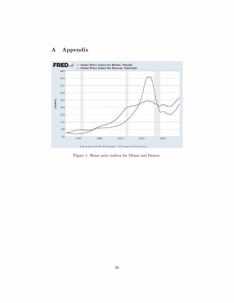
A Appendix

Figure 1: Home price indices for Miami and Denver.

20