CEP Discussion Paper No 588 (Revised from November 2003)

March 2006

Trade and Economic Geography: The Impact of EEC Accession on the UK

Henry G. Overman and L. Alan Winters

Abstract This paper combines establishment level production data with international trade data by port to examine the impact of accession to the EEC on the spatial distribution of UK manufacturing. We use this data to test the predictions from economic geography models of how external trade affects the spatial distribution of employment. Our results suggest that accession changed the country-composition of UK trade and via the port-composition induced an exogenous shock to the economic environment in different locations. In line with theory, we find that better access to export markets and intermediate goods increase employment while increased import competition decreases employment. Keywords: Economic geography, EEC, UK manufacturing JEL Classification: F15, F14, R12 This paper was produced as part of the Centre’s Globalisation Programme. The Centre for Economic Performance is financed by the Economic and Social Research Council. Acknowledgements We are grateful to Sandra Bulli and Andrea Molinari for research assistance and the ONS Business Data Linking Project for facilitating access to the ARD. The work was largely undertaken while Alan Winters was at the University of Sussex and a senior visitor at the CEP. The paper has benefited from comments by seminar participants at the CEP and at two CEPR conferences in Cagleiri and Paris. This work contains statistical data from ONS which is Crown copyright and reproduced with the permission of the controller of HMSO and Queen's Printer for Scotland. The use of the ONS statistical data in this work does not imply the endorsement of the ONS in relation to the interpretation or analysis of the statistical data. This work uses research datasets which may not exactly reproduce National Statistics aggregates. Financial support from the ESRC (grant number L138251028) is gratefully acknowledged. Henry G. Overman is a member of the Centre for Economic Performance Globalisation Programme and a lecturer in Economic Geography in the department of Geography and Environment at the London School of Economics. He is also affiliated with the Centre for Economic Policy Research' s International Trade Programme. Email: h.g.overman@lse.ac.uk L. Alan Winters is Professor of Economics at Sussex University and a Senior Research Fellow in the Globalisation Programme at the Centre for Economic Performance, London School of Economics. He is also Director of the Development Research Group at the World Bank. Published by Centre for Economic Performance London School of Economics and Political Science Houghton Street London WC2A 2AE All rights reserved. No part of this publication may be reproduced, stored in a retrieval system or transmitted in any form or by any means without the prior permission in writing of the publisher nor be issued to the public or circulated in any form other than that in which it is published. Requests for permission to reproduce any article or part of the Working Paper should be sent to the editor at the above address. © H. G. Overman and L. A. Winters, submitted 2006 ISBN 0 7530 1666 4

2

1. Introduction Work in international trade has long been concerned with what is produced where. That is, in the distribution of economic activity across countries. In contrast, this paper forms part of a small, but growing literature focusing on the relationship between economic integration and the spatial distribution of economic activities within a country. We view UK accession to the European Economic Community as a trade “shock” and use this shock to help identify how trade affects the spatial distribution of activity. The UK’s accession to the EEC is a good case study for assessing these trade effects. First, as discussed below, that the UK would join was far from certain until less than a year before accession. This means that we can expect firm responses to come after UK accession even if firms are forward looking. Second, accession occurred when tariffs, generally, were at much higher levels than today. The fact that tariff reductions were large means that impacts should be easier to identify. Third, these tariff changes affected most manufacturing sectors at a time when manufacturing was a significant component of the UK economy. As most studies, ours included, focus exclusively on manufacturing, the relative importance of this sector will matter for the magnitude of any general equilibrium effects of liberalisation. Fourth, we are able to use detailed data on individual firms and the ports through which trade flows. This allows us to test the predictions from economic geography models in an original fashion. Finally, the existing literature focuses on the response of developing countries to major trade liberalisations. See, for example, Hanson (1996, 1997, 1998), Pavcnik (2002) and Tybout (2000, 2001). Studying developed countries, however, has one key advantage over looking at developing countries. Frequently, developing country liberalisations form part of a larger package in response to macroeconomic shocks. In contrast, although the early 1970s was a time of significant macroeconomic shocks, accession was not a response to these shocks. Thus, we can treat accession as providing a natural experiment in terms of changing trade policy. The fact that UK accession to the EEC led to a significant re-orientation of trade towards EEC members is well documented elsewhere - see, among many others, Winters (1984), or Begg et al (2003). Less well known, is the significant re-orientation in terms of the port through which this trade occurred. We describe this re-orientation in Overman and Winters (2005). In this paper, we argue that because this changing port-composition was a result of accession it induced different exogenous shocks to the economic environment in different UK regions. We then examine whether the resulting changes to the spatial distribution of employment are in line with predictions from models of economic geography. To do this, we construct a panel of firms for which we know production sector, employment and the Travel To Work Area (TTWA) where these firms are located. We use data on the volume of trade by port and distance from these ports to different TTWAs to construct measures of the import competition and access to export markets and intermediate goods faced by firms. Using the panel nature of our data to control for unobserved firm specific effects, we then test whether these three access variables have a significant impact on firm employment. Of course, it is possible that changes in firm employment actually drive changes in these variables rather than vice-versa. We argue, however, that the changing country composition of UK trade during this period is driven by accession, not the performance of individual firms and so we can use this changing country composition to instrument for the three access variables. The rest of the paper is structured as follows. Section 2 provides a summary of the historical background and details the extent of trade liberalisation that occurred when the UK joined the EEC. Section 3 considers theoretical predictions about the possible impact of integration on the spatial distribution of activity. Section 4 details the trade and production data that we use. Section 5 constructs measures of import competition, export market access and intermediate good market access and analyses whether these have the predicted impact on firm employment. Section 6 looks at the extent to which changes in the port composition of trade are determined by the country composition of trade. Section 7 then uses

3

these findings to construct instruments for the port composition of trade and thus assess whether the effects that we document in section 5 are actually due to the trade liberalisation associated with accession. Section 8 concludes.

2. The background The UK first applied to join the EEC in 1961. This application, and a second in 1967, failed as a result of a French veto. A third application was successful and the UK joined on 1st January 1973. For our purposes, it is interesting to note that even without the French veto, UK membership was far from certain. Edward Heath’s narrow majority of 30 was sufficient to ensure that parliament accepted the government’s accession terms, but the signing of the Treaty of Accession was a much closer run thing. In the end, the government carried the day with a majority of 21. As suggested above, this uncertainty ensures that adjustment to accession is likely to have occurred after entry rather than before, even if firms are forward looking. Moreover, once the need for adjustment has been identified, it is likely to take a while to effect, so we should observe the impact in our data (which start from 1970).

Table 1: Major Economic Events 1970s

Year Month Event 1971 February Decimal currency introduced August End of Bretton Woods era; Pound allowed to float 1972 January Miners begin pay strike February 3 day working week begins for most industry to conserve power supplies; miners

return to work May Sterling joins the EEC currency snake June Sterling out of the snake November Counter inflation bill – 90 day standstill pay, prices, rents, dividends 1973 January UK joins EEC; further controls on prices, pay, rents, dividends March Pay Board and Price Commission established May 1.6m workers strike against counter-inflation measures October 66% price increase light crude oil November 25% cut in oil supplies to West; voltage reductions due to power engineers

industrial action; petrol ration coupons issued 1974 January Light crude oil price from $5 to $11.5 per barrel; 3 day working week February Miners strike March End of miners strike and return to 5 day working week May Lifting of restrictions on fuel July TUC accept voluntary wage restraint in place of statutory wage controls 1975 August £6 per week pay rise limit becomes effective October OPEC 10% price increase July Heavy selling of sterling 1976 September Treasury announces it will seek $3.9bn loan from IMF January Further $3bn loan from Bank of International Settlements 1977 July Abolition of tariffs with EFTA December OPEC announces new 14.5% (staggered) price increases 1978 January “Winter of Discontent” – series of strikes in public services 1979 May Price Commission abolished June OPEC announce 15% price increase

Notes: The timeline is an extract from that available at http://www.bized.ac.uk

4

While this uncertainty works in our favour, other macroeconomic uncertainties of the time do not. A number of these uncertainties were global, some were UK specific. Table 1 provides a timeline of major events. These events are likely to have an impact on the composition of overall economic activity. However, our focus is on the impact that integration has on the spatial distribution of economic activity in different sectors within the UK taking the level of aggregate sectoral activity as given. It is still possible that these shocks could account for what we observe, but only if they affect locations asymmetrically in a way that is correlated with the trade shocks we identify. Given their macro-economic nature, this seems unlikely, but clearly the possibility cannot be completely ruled out. We finish this brief background review with a note on the changes in tariffs associated with accession. In the early 1970s tariffs were considerably higher than now, so that the margins of preference generated by accession were, in some cases, quite large. Table 2 reports average UK and EEC tariffs after the Kennedy Round – i.e. applicable from 1972 to 1980 when the Tokyo Round started. In 1972 UK imports from outside the Commonwealth and manufactured imports from EFTA faced the tariffs reported in the ‘UK’ column, with a mean of 7.2% but entries as high as 19%. By 1979 all except those from the EEC, EFTA (manufactures) and the ACP developing countries faced the tariffs in the ‘EEC’ column, with mean of 4.2% and peaks of 14%. The excepted countries faced zero tariffs broadly speaking.

Table 2: UK/EEC Tariff rates 1972-1979

Product UK EEC UK EEC Mineral products 0.2 0.1 Footwear and headwear 14.7 12.4Chemical products 8.1 6.9 Stone, ceramic and glass products 10.2 8.0Rubber products 7.4 2.0 Base metals and metal products 5.2 4.2Hides, furs, leather products 4.6 1.3 Unwrought, pig iron, scrap 1.1 2.0

Raw hides, skins, fur N/A N/A Basic shapes and forms 8.9 7.0Articles of leather, fur 13.1 1.3 Steel 9.2 6.7

Wood and cork products 2.3 1.1 Other 7.5 8.7Wood, natural cork 0.5 0.1 Articles of base metal, misc. 10.0 7.1Articles of wood, cork 6.8 9.4 Nonelectrical machinery 8.6 6.4

Pulp and paper 7.8 6.9 Electrical machinery 12.4 9.1Pulp 0.1 2.5 Transportation equipment 9.8 9.3Paper 13.1 11.1 Precision instruments 13.5 8.4

Textiles 9.1 4.7 Miscellaneous 4.2 2.4Natural fiber and waste N/A 0.2 Yarn and basic fabrics 15.0 11.1 Special fabrics, apparel, other 19.0 13.9

Total 7.2 4.9

Notes: N/A denotes figures not available in the original source. Source: Preeg (1970).

3. Theory What should we expect to be the impact of accession on the spatial distribution of economic activity in the UK? Obviously, theories of comparative advantage help us to understand the changing composition across sectors, and this must play a part in the overall decline in UK manufacturing during this period. It could also clearly help us to understand changes in the distribution of aggregate activity if regions are specialised in sectors that perform differently as the UK adjusts to accession. However, our focus is on how integration affects the spatial distribution of activity within particular sectors, on which theories of

5

comparative advantage are essentially silent. Thus the theoretical foundation that we use comes from the literature that directly considers the impact that integration has on economic geography. These effects have been the focus of the recent ‘New Economic Geography’ (NEG) associated with urban and international economists, see Fujita, Krugman and Venables (1999), Fujita and Thisse (2002), and Baldwin, Forslid, Martin, Ottaviano, Robert-Nicoud (2003) for overviews. The analysis of NEG formalises ideas about the impact of trade from an older literature associated with economic geographers. This literature argues that the equilibrium spatial distribution of economic activity depends on the balance between agglomeration and dispersion forces. Firms that locate in big markets benefit from being close to their customers and suppliers. That is, they benefit from demand and supply linkages. Offsetting these advantages is the fact that big markets are more crowded which increases product and factor market competition putting downward pressure on prices and upward pressure on wages.1 The balance of these forces depends on the trade costs between different locations. At higher trade costs, the costs of serving distant customers are so large that they dominate the agglomeration forces and activity is dispersed. At intermediate trade costs, the opposite is true and agglomeration can occur, while at low trade costs, congestion costs are dominant and industry may once again disperse. What do such models imply for the economic geography of the UK as it opens up to trade with Europe? One possibility is that regions that are close to new trading partners (i.e. “border” regions), benefit disproportionately from the improved market access that comes with accession. Hanson (1996, 1997, 1998) has used regional data from Mexico to test whether changing export market access helps explain the changing economic geography of Mexican regions. He argues that the formation of NAFTA acts as a natural experiment that disproportionately increases the export market access of regions in the north of the country close to the US border. His empirical work tests the prediction that this change should lead activity to relocate from Mexico City to the northern regions driving up employment and wages there. Both of these predictions hold true.2 The effect found by Hanson is not the only possibility when a country opens up to trade. While export market access and access to imported intermediate goods rises in border regions, so too does the degree of product market competition felt via imports. Hanson focuses only on export market access and thus argues that the employment share of border regions must rise. Once we allow for increased import competition, border regions may suffer if activity relocates from those border regions to other non-border regions. This happens because firms in non-border regions are partly protected from increased competition by the fact that imports incur higher transport costs to reach those regions. This line of reasoning has been formalised by Alonso-Villar (2001), Monfort and Nicolini (2000), Paluzie (2001) and Crozet and Koenig (2002). Brulhart and Koenig (2005) provide related empirical evidence for quite aggregate sectoral data (the 8 sectors of 1 digit NACE) for the CEEC countries. When we turn to our empirical analysis we view ports as identifying the borders of the UK (i.e. the points through which imports enter and exports leave). We then construct variables that capture all three access effects. We expect activity to rise with better export market access and access to intermediate goods and to fall with increased import competition. The reduced form relationship we estimate is close to, but not exactly, that which could be derived from extending the formal models mentioned above to allow for multiple sectors. As data limitations prevent us from estimating a more structural equation, we see little to be gained from working through a more formal model. Instead, we motivate our approach on the basis of

1 In NEG models that rely on Dixit-Stiglitz production functions this is technically a market crowding effect and not a product market competition effect. See Ottavianno and Thisse (2003) for further discussion. 2 Hanson’s results may also be influenced by the general, non-discriminatory, liberalisation in Mexico which Krugman and Livas (1996) argue should reduce the attractions of the metropolis – Mexico City – relative to other locations.

6

the informal reasoning and the intuitive predictions that we have drawn out above and refer the interested reader to the references given.

4. Data 4.1 Production data Our basic unit of observation will be the employment of UK manufacturing establishments for the period 1970-1992 constructed using production data from the Annual Respondent Database (ARD).3 The ARD is an extremely rich data set which contains information about all UK manufacturing establishments.4 Griffith (1999) provides a detailed description of this data. Establishments provide data on a range of variables, although the data available on any particular establishment in any given year depends on whether it was selected to make a detailed return that year. Selected establishments answer a detailed questionnaire providing data on a range of variables. In contrast data for non-selected establishments is much more basic. As a general rule all larger establishments with more than 100 employees are selected, as are a percentage of establishments with more than 20 but less than 100 employees. Establishments with less than 20 employees are usually exempt (non-selected). The precise rules vary year by year. Table A1 in the Appendix provides details of the sample selection criteria for all years between 1970 and 1992. For our analysis we work with employment data, rather than wages, because we are confident that employment variables are constructed in a consistent way across time.5 We then need to decide which of two possible variables to work with. One possibility is the estimate of employment that is used when deciding which establishments are selected to return a full questionnaire.6 Somewhat confusingly, the ARD refers to this as selected employment. Selected employment should be recorded whether or not an establishment makes a full return (given that it forms the basis for deciding which establishments have to make such a return). Although this is true from 1980-1992, it is not so in the 1970’s where employment has been collected, but (accidentally) deleted for non-selected establishments. As a result, we choose only to work with returned employment. For an establishment to be in our sample, we must have returned employment for at least two years during our sample period.7 Given the sampling frame discussed above, this means that our sample will be composed of a disproportionate number of larger establishments. Below, we present robustness checks that show that this sample selection does not affect our results.

3 The availability of trade data restricts us to only study 1970-1992. We discuss this below. 4 For legal reasons, we exclude Northern Ireland. The smallest unit of observation in the ARD is the local unit (‘plants’). Local unit data is not available for the 1970s. In addition, allocating plants to the regions that we use, Travel To Work Areas (TTWA), would be a huge undertaking. Instead we use data for reporting units (‘establishments’). Reporting units may consist of several local units. The calculation of access variables is problematic for reporting units with local units in different locations. Given the data problems discussed above, we proceed by assigning all employment to the reporting unit, ignoring redistribution across local units. If anything, this means that we understate the impact of accession if re-allocation across local units is affected in the same way as that across reporting units. Fortunately data from 1997 (when the ARD provides TTWA for local units) show this problem only affects a small percentage (3% in 1997) of reporting units because less than 10% of them have multiple local units and less than a third of these then have local units in different TTWAs. Reporting units may also be part of a larger enterprise group but we ignore any correlation for units that are part of the same group. 5 In the terminology of Head and Mayer (2004a) we consider the quantity version of the market size and product competition effects rather than the price (or wage) version. 6 This employment data is obtained from the various predecessors to the Inter Departmental Business Register and the data may have come from a return to another survey or an administrative source such as VAT or PAYE. 7 We need at least two years to estimate firm specific fixed effects. We also only consider firms that do not change sector.

7

Given that our unit of observation will be employment by establishment, we need to be able to classify establishments by activity and location. All establishments are classified according to their main economic activity using the Standard Industrial Classification (SIC). During our sample period, the SIC changes from SIC 1968 revision (SIC68) to SIC 1980 revision (SIC80). A preliminary mapping from SIC80 to SIC68 was provided by the ONS and then supplemented using ARD data on individual establishments’ sectoral classifications. For compatibility with the trade data, we then map from SIC68 to the Industry/Commodity group classification used in the 1974 IO table (IO sectors). IO sectors are basically defined at, or are aggregations of, 3-digit SIC68 sectors (minimum list headings). Details of the mappings from SIC80 to SIC68 to IO sectors are available from the authors on request. The list of the 80 IO sectors that we work with in the econometric section are given in table A2 of the Appendix. Establishments can be located using a number of indicators. All establishments can be located in one of 10 UK regions. However, to analyse the impact of integration, we wanted to use a smaller geographical scale that would hopefully provide more cross-section and time series variation with which to identify the effects. After much experimentation, we constructed a consistent set of geographical units across our time period based on 307 UK Travel To Work Areas (TTWA 1998 revision). Allocating establishments to TTWAs is complicated because the location information provided in the ARD varies significantly over time. The three most important sources of location information are the establishment’s local employment office, local authority and postcode. Local employment codes are provided at the start of our time period but not the end. The timing is reversed for postcode. Again, detailed information on how establishments are located is available on request. One issue for estimation arises from the need to reconstruct establishment TTWA from a variety of location variables that are not perfectly nested: Sometimes, establishments close to the boundaries of TTWA may change TTWA even though the establishment has not relocated. Given this, we do not explicitly model establishment re-locations, instead assuming the same establishment level fixed effect independent of any relocation. For establishments that change TTWA due to the imperfect mapping of location variables to TTWA this introduces some noise in the measurement of the access variables, but should not affect results otherwise. Genuine moves should not affect our results either, unless they are driven by changes to establishment fixed effects that are systematically related to the choice of new location (and hence the measure of access variables). This seems unlikely. Similarly, although we allow for establishment births and deaths (i.e. the panel is unbalanced) we do not explicitly model the extent to which accession changed birth and death rates across TTWA. 4.2 The International trade data8 The main international trade data that underpin our analysis describe UK trade by port and commodity from 1970 to 1992.9 The dataset was specially constructed from official sources for the present exercise and, to our knowledge, these sources have never been exploited before at this level of detail. They were supplemented by data for the same commodities and time period on the sources of imports and destination of exports, which reflect the re-orientation of UK trade following accession to the EEC. Data on UK trade by port have been published in a variety of sources since 1970.10 The source data contain three major omissions: export data for 1983, both export and import data for 1987, and export

8 Some of the material in this sub-section is taken from section 4 of Overman and Winters (2005). 9 Data are not available by port for trade with the EU after 1992 because under the Single Market Programme these flows were treated as internal European trade and were recorded via VAT returns rather than by Customs and Excise at the port. 10 The Annual Statement of Trade, Vol. V, (HM Customs and Excise), 1970-75; Statistics of Trade through United Kingdom Ports, (HM Customs and Excise), 1976-80; on micro fiche, 1981-87, and then electronically for 1988-92 via the commercial data suppliers, Business Trade Statistics Ltd.

8

data for HS chapters 84-99 for 1989-90. The structure of the data varies by publication and the classifications evolve from SITC(R) through SITC(2R) and (3R) to the Harmonised System (HS, 1988).11 We have attempted to correct for these evolutions and to convert the data to a common classification. The latter process requires some approximation, usually based on the structure of UK total trade. The most disaggregated continuous series that could be constructed was at the Division (2-digit) level of the SITC(R), which distinguishes 56 headings, of which we have to drop one (35, gas and electricity) and combine one pair into a single heading (33 and 52 which become entwined in the later classifications). At this level no volume or deflator data are available, so all data are in value terms. Given the high rates of inflation over much of the period this renders inter-temporal absolute comparisons meaningless, but for our purposes using ports’ shares in total UK trade of a commodity is sufficient. Over the period 1970-92 data are reported for about 120 ports at some point of time. However, the coverage changes through time and there is a fairly continuous process of re-combination of ports into local groups, as the geographical responsibilities of individual customs offices evolved. In most cases we solve these problems by aggregating ports into groups that are invariant over time, but there remain a number of minor inconsistencies.12 We do not believe that we have introduced any major errors, however. Overall we are able to compile consistent data on 92 ports or local groups of ports over 1970-92.13

When we turn to the econometric specifications, it is sometimes useful to group ports into eleven groups, loosely based on those used by Chisholm (1992, 1995) in the only previous analysis we know of that considers the effects of accession on the geography of trade (but not production). The eleven groups, along with the acronyms that we use to refer to them, are defined in table A3 of the appendix. The grouping is more finely disaggregated around the South East, because we expect integration to affect those ports in particular.14 4.3 Mapping Trade Flows to Industries The data on trade flows prior to 1977 are available only at Division (2-digit) level of the SITC(R). Thus all subsequent data were converted to this basis. To relate these data to manufacturing establishments we need to develop a concordance between SITC(R) and UK IO sectors. No such converters were published, so we had to proceed indirectly. Aki Kuwahara of UNCTAD kindly supplied us with a ‘universal’ concordance between eight classifications including the SITC(R) and the International SIC68 from which we generated a mapping from the approximately 1,200 basic SITC(R) 4- and 5-digit headings to 4-digit ISIC headings, of which there are one hundred of relevance for trade in goods. This mapping was then matched to UK visible export data by SITC(R) collected from the UN Comtrade Database,15 averaged over 1970-80. In about a dozen cases an SITC heading was mapped to more than one ISIC heading, in which case trade was divided evenly between those headings. In about three dozen

11 In addition to classifying goods differently, the classifications also have different coverage of goods. E.g. variations in the treatment of non-monetary gold, tax-free cars, and parcel post. 12 E.g. Avonmouth was included in Bristol 1970-73, the two ports were separated for 1974-80 and after 1980 Bristol disappears as an explicit entry and we take it implicitly to be included in Avonmouth. 13 The data have been subject to a number of consistency checks as they have been prepared, including checking against independent sources. Unfortunately a small number of implausibilities remain in the allocation of trade across ports. The most serious remaining mystery is the sharp changes in the share of exports of engineering goods (SITC(R)7) passing through Heathrow in 1991. We have been unable to explain this or to find a plausible way of adjusting the data. 14 We separate London from THAKE and Felixstowe from HAVEA because the two named ports are major specialist deep-sea ports which may have different trading roles from their regional neighbours. We do not treat Southampton specially, because it entirely dominates its region, nor Liverpool, because we are less interested in the North-West region a priori. 15 For which, thanks are due to Azita Amjadi of the World Bank.

9

cases an SITC heading had not been mapped to ISIC. Most of these were UN ‘special’ 4-digit codes ending in zero which are used when official statisticians cannot allocate trade across 4-digit headings but know its 3-digit category. Most of these actually recorded no trade for the UK, and so allocating them to ISIC did not matter, but this was not always the case. In addition, there were about half a dozen ‘genuine’ SITC heading that were unmapped. In these cases we created a mapping from the textual descriptions of the two classifications.16 The dataset resulting from these manipulations comprised about 1,200 rows each containing an ISIC heading, a SITC(R) heading and an export flow. This was then aggregated into SITC(R) 2-digit divisions and then into the ISIC headings to create a matrix of trade cross-classified by ISIC and SITC(R) sections. From this the converter matrix Bx was created by dividing entries by their column sums. Thus Bx reports how exports of an SITC section flow are derived from ISIC 4-digit headings. A corresponding matrix was created for imports, BM, using UK imports data from the same source averaged over 1970-80. Department of Industry (1980) defines UK Input-Output (IO) sectors in terms of the minimum list headings (MLH) of the UK’s SIC68. There are 91 sectors which potentially could produce tradable goods. CSO (1971) concords the MLHs with ISIC 4-digit categories, noting the many places in which the concordance is less than perfect. Most of these are small enough to ignore or are neutralised when MLHs are aggregated into IO-sectors. Thus the mapping normally maps the whole of an ISIC heading into a single IO-sector. However, thirteen major conflicts between ISIC and SIC are explicitly listed in the introduction to CSO(1971);17 these were treated individually wherever possible, as were the 26 cases in which an ISIC heading is mapped to more than one IO-sector. In these cases, we reverted to the SITC(R) 4- and 5-digit trade data to divide the ISIC trade aggregate appropriately between IO-sectors, completing separate exercises for exports and imports. The resulting matrices, CX and CM, report how trade flows by ISIC heading may be allocated across IO-sectors. Once the classification matrices have been derived we apply them to the data on SITC(R) Division trade by port to create series of trade by port, IO sector and year, which we can marry with the establishment data.

5. Import competition, access to export markets and the changing economic geography of UK manufacturing In an earlier paper (Overman and Winters, 2005), we describe the way that accession re-orientated UK trade towards ports that were close to EEC member countries. Re-orientation did not occur uniformly across sectors. Some sectors showed particularly strong re-orientation while the effect in others was weaker or even went in the opposite direction. In this paper, we use this cross-sector variation to examine whether accession helps to explain changes to the economic geography of UK manufacturing. The hypotheses that we investigate are (i) accession re-oriented UK trade by country of origin/destination and that this caused a re-orientation in terms of the ports used for that trade; (ii) that this changed the degree of import competition, and the ease of access to intermediate goods and export markets faced by establishments in different TTWAs; (iii) these changes in turn affected the economic geography of manufacturing. We proceed in several stages. First, in this section, we describe how we calculate import competition, access to intermediate goods and export market access for TTWAs. We then show that changes in these measures are correlated with changes in establishment employment in a way that is consistent with theory. In the following two sections, we then consider issues of causality.

16 Finally, two SITC headings were mapped to a ‘false’ ISIC heading, 9999; that is, for these headings there is no corresponding ISIC heading at all. This ‘false’ heading was treated symmetrically with genuine ISIC headings. 17 This is in addition to a general note about the different treatment of repair work in the two classifications, which we cannot make allowance for.

10

Our dependent variable is establishment employment. We know the industrial sector of the establishment and in which TTWA they are located for the time that the establishment exists during the period 1970-1992.18 We want to explain the evolution in establishment employment in terms of import competition, access to intermediate goods and export markets. We start by using the port trade data to construct proxies for these three access variables. Although we have trade data by ports, we do not have information on the UK origin of exports and the UK destination of imports. One possibility is to assume that imports and exports occur only through the closest port. That is, assume that ports have well defined ‘hinterlands’ and ‘forelands’. Evidence presented in Hoare (1977, 1985, 1986, 1988) and Chisholm (1992) argues against this. Chisholm reports Hoare’s results as showing that “if we take the standard region as the geographical unit of analysis, then in 1964, the tonnage of [firm] exports routed through a port in the same standard region accounted for 63% of the total; by 1978 the proportion had fallen to 48%” [Chisholm 1992, p563]. Chisholm’s results suggest that “the rapid reduction in the strength of local linkages seems to have abated in the period 1978-86” [Chisholm 1992, p563]. Given that on average establishments are not only linked to their closest port we instead assume that distance from all ports and the volume of trade through those ports are the key determinants of the access variables. Thus, we assume that establishments in TTWAs that are close to ports with large amounts of imports face more import competition than those in TTWAs a long way from these ports. Similarly for intermediate goods and export market access. It is important to note that such a formulation is consistent with NEG theory where love of variety means that consumers purchase all varieties of differentiated manufactured goods, while establishments supply their differentiated goods to all markets. Given that different ports tend to trade with different foreign markets (something we consider empirically below), the idea that distance to all ports matters is consistent with the underlying theory. Using this assumption, we construct a measure of import competition faced by an establishment in a given sector located in a given TTWA as:

∑= plp

jptjlt d

mIMP

where mjpt is the share of imports for sector j coming in through port p at time t and dlp is the distance in kilometres between port p and TTWA l. To implement this equation, we map trade flows to IO sectors as described in section 4.3. Distance are calculated as straight line distances using data on the eastings and northings of the port and the centre of the TTWA. For the moment, we weight port trade flows by the simple inverse of distance, but we discuss other alternatives in section 7.2 below. We calculate export market access equivalently:

∑= plp

jptjlt d

xEXP

using the share of exports (xjpt) that leave the UK through each port. To calculate intermediate market access we weight the imports in different sectors coming in at each port by industries use of that sectors good in production. That is, our measure of intermediate good market access is:

∑ ∑=k p

lp

kptjkjlt d

maINT

where ajk is industry j’s use of intermediate k.19

18 As discussed in the data section, we only consider firms that do not change TTWA or IO sector during the life of the firm. 19 Industry j’s use of intermediate k is taken from Department of Industry (1980).

11

Using these measures of import competition, intermediate good and export market access, we run the following regression for each sector for the panel of employment by establishment.

itijltjjltjjltjjit cINTEXPIMPe εββββ +++++= )ln()ln()ln()ln( 3210 where eit is employment in establishment i, ci is an establishment specific fixed effect, εit is an idiosyncratic shock; IMPjlt is the measure of import competition for sector j (the main economic activity of establishment i) in TTWA l (where establishment i is located) at time t, with intermediate good and export market access defined similarly. The betas are coefficients to be estimated. We estimate the specification by sector (so that coefficients vary across sector) using data from 1970 to 1992. We exclude data from 1983 (no export data) and 1987 (no export or import data). We include, but do not report results for, a set of year dummies. Theory predicts a negative coefficient on import competition ( 01 <iβ ), and positive coefficients on intermediate good and export market access ( 02 >iβ and 03 >iβ ). A few comments are in order. First, we observe no additional information at the establishment level so all we can do is use the panel dimension of our data to control for the unobserved establishment specific fixed effect. Second, the only explanatory variables we can measure at the TTWA level over this period are the access variables included in the specification. Third, the flow of trade through different ports may be partly driven by changes in the spatial distribution of UK manufacturing. To control for these problems we will present instrumental variable results in section 7, once we have considered the extent to which the direction of trade determines the port composition. Instrumenting controls for the problem of the endogeneity of the included TTWA variables. Providing that other TTWA level or establishment level variables are uncorrelated with the country re-orientation of trade (which seems reasonable) this should also control for other omitted variables that might be correlated with the access variables. For the moment, table 3 reports results from estimating the specification using the within estimator, ignoring these three problems.20 We get the clearest results on export market access. 21 coefficients are positive and significant at the 5% level or higher, with only 10 negative and significant and the rest insignificant. Results on import competition and intermediate good access are more mixed. For import competition, 16 coefficients are negative and significant in line with theory, while 13 are significantly positive. For intermediate access, 16 coefficients are positive, in line with theory with 12 negative. Part of the problem here is that the diagonal coefficients on the input output table are often large at the two digit level so these two variables are quite highly correlated. On balance, we would argue that our initial results are more with the theory than against it, but we postpone further discussion until we have dealt with the three problems highlighted above. This is the issue to which we now turn using the fact that UK accession acts as a natural experiment which changes the direction of trade independent of changes to UK economic geography and thus provides a way to construct a variable to instrument the economic geography variables. Details of how we construct the instrument are given in section 6, while section 7 considers results when we use these instruments in our basic panel specification.

20 There are insufficient observations for sector 61 (other vehicles). No industry is classified in sector 74 (textile finishing). It is not clear why this is the case, but this is true in the raw data and is not a result of our processing of the data.

12

Table 3: Estimates of effect of economic geography variables on establishment employment

IO IMP EXP INT N IO IMP EXP INT N 10 -0.18 0.36 -0.14 40 50 0.31 -0.19 0.06 21511 0.49* 0.15** -0.55** 130 51 -0.20** 0.14* 0.10 92612 -0.20* 0.02 0.17* 149 52 16.04** 1.73** -18.06** 22313 0.03 0.03 -0.06 1258 53 0.61** 0.06 -0.70** 30814 -0.71** 0.09 0.72** 1031 54 -0.72** 0.21* 0.67** 52915 -0.09 0.04 0.16 512 55 -0.11 0.04 0.12 25216 -4.33 0.30** 4.23 39 56 0.00 0.12 -0.07 74617 -0.01 -0.13** 0.02 215 57 -0.18** 0.31** -0.04 82518 -0.01 -0.12** 0.23** 375 58 0.13 -0.03 0.32 5919 -0.01 -0.04 0.10 121 59 0.00 -0.13** 0.06 152920 0.34** 0.06 -0.31** 798 60 -0.01 0.08 -0.03 57921 0.00 0.09 0.07 326 62 -0.04 0.04 0.00 108322 0.04 -0.10** 0.22** 337 63 -0.40 0.18* 0.26 49223 0.50** -0.18* -0.35** 32 64 -0.53** 0.25* 0.42** 32124 0.03 0.12** 0.04 609 65 0.03 0.02 0.06 34825 -0.08 0.10 0.04 290 66 0.26* -0.23* 0.13 13826 0.09 -0.08 -0.08 161 67 0.06* 0.03 -0.05* 484027 0.02 0.01 0.01 213 68 0.00 0.09 -0.16 5628 -0.38** 0.45** 0.27* 111 69 -0.76** 0.01 1.02** 71329 0.12 -0.27** 0.21** 422 70 0.08 0.05 -0.21* 80830 -0.25 -0.01 0.11 75 71 0.40 0.20* -0.36 103031 -0.07 0.19 -0.04 67 72 0.50* -0.08 -0.62** 16632 -0.09 0.09 0.03 434 73 0.13 -0.19 -0.10 27533 0.10* 0.12* -0.07 673 75 -0.33* -0.31* 0.58** 16534 0.07 0.03 0.00 751 76 0.03 0.04 -0.02 73335 -0.35 0.00 0.64* 418 77 0.11** 0.00 -0.13** 391836 0.04 0.16** -0.07 492 78 0.13* -0.02 -0.01 53537 0.45* 0.01 0.03 229 79 -0.12 0.20** -0.10 43738 0.02 -0.11 0.17 628 80 -0.13* 0.13* 0.13 67939 -0.10* 0.04 0.09* 591 81 -0.01 -0.17 -0.27 3140 -0.75** 0.14 0.85** 97 82 -0.04 -0.01 0.11** 135341 -0.22 0.53** -0.23 244 83 -0.06 0.09* 0.07** 165042 0.02 -0.11* 0.08 877 84 0.50 -0.02 -0.46 322043 0.97 0.10 -1.27 102 85 0.65 0.22** -0.82 32444 -0.09** 0.01 0.05 2269 86 -0.13 0.04 0.12 84345 -0.10** 0.24** -0.08* 1770 87 -0.08 0.02 0.02 83046 0.01 -0.05 0.09** 2347 88 0.04 -0.09** 0.00 497947 -0.19** 0.20** 0.04 1655 89 0.00 0.07 0.00 53548 0.04 0.00 -0.11** 941 90 -0.07 -0.02 0.03 215549 -0.30* 0.80** -0.16** 171 91 0.10* -0.12 -0.01 1323

Notes: The dependent variable is returned employment at the establishment level. IO gives the IO sector number, see table A2 in the appendix for sector names. IMP reports the coefficient on import competition, EXP the coefficient on export market access and INT the coefficient on access to intermediate inputs. N gives the number of unique establishments used to calculate the within estimator. * denotes significant at 5%, ** significant at 1%. All specifications include establishment fixed effects and time dummies. Data is for 1970-1992 (excluding 1983 and 1987). Source: Authors own calculations using ARD data and trade data described in Section 4.

13

6. Explaining the Port-Composition of UK Trade Our basic hypothesis assumes that the direction of trade partly determines the port-composition of trade and that the direction of trade is exogenously shifted by UK accession. This section considers this hypothesis, first for the sake of its intrinsic interest, but second in order to use the direction of trade as an instrument for the port-composition in our estimating equation. We are not arguing that direction is the only factor behind the port-composition of trade. Clearly factors such as port-facilities, internal transportation links and traditional shipping lines also matter. However, even the most casual reflection on shipping routes suggests the likelihood of some link – for example, roll-on, roll-off ferries for France leave mainly from South-East England, while those for Ireland leave from equivalent facilities in Wales, North-West England and West Scotland. We explore the substantive question using data for 11 port-regions and 54 commodities.21 The hypothesis concerns the ‘behaviour’ of ports and hence we treat ports as the basic observational units and estimate, for each, a panel of 54 commodities with 21 years of data for exports and 22 for imports. We are interested in the shares of each commodity entering/leaving via specific ports which is convenient, since by converting everything to shares we avoid the need to allow for inflation. The basic equation is:

∑= D

d gdtpdpgt TbS

where subscripts are p for port group, g for commodity, t for time and d (d=1,…,D) for destination of exports (or source for imports). S is the share of the port group p in total trade in good g in year t, and T the share of destination d in that trade. Because the shares sum to unity over d (i.e. 1=∑d gdtT , all g and t), the equation is rewritten in the form:

gDD

d gDtgdtpdpgt bTTbS +−=∑ −1 )(

where D refers to the Dth destination. Further, because the shares all sum to unity over ports ( 1=∑ p pgtS ,

all g and t), the gdb sum to zero over p and the gDb to unity. Provided that all equations contain the same regressors and no observations are omitted, these conditions are automatically satisfied by linear regressions run on each port separately. In addition we include a time trend in the equations to capture slowly evolving factors affecting ports (allowed to vary over port-regions and over commodities), and a dummy variable taking the value of unity from 1980 onwards to represent the abolition of the National Docks Labour Scheme. This highly restrictive labour agreement applied in around half of UK ports, and is widely regarded as having curtailed their productivity and growth relative to non-Scheme ports. The coefficients of these variables also sum to zero over port groups. We are interested in trade with Western Europe as a factor in UK economic geography, and also note that for very distant partners (e.g. China) the choice of UK port is likely to depend very little, if at all, on its closeness to that partner. Hence given the likely difficulties of identifying very many country effects, we distinguish the following countries, or groups of countries as sources for imports and markets for exports: France; Germany; Benelux ;Scandinavia; Italy; Austria and Switzerland; Other Western Europe, and Rest of the World (which is the omitted category, D, in the estimating equation above.)22 Given that our

21 Given that we do not have a full model of the port composition of trade we do not try to explain the small number of zero-flows for regions. Rather we take them as data, omitting them from the sample, and omitting all observations for a region-commodity pair if it can muster fewer than five observations exceeding 0.000001 over the sample period. 22 Trade data aim to identify the ultimate destination of exports and the actual producer of imports rather than country to or from which they are immediately transported. Thus some trade recorded as bound to or from a country may actually travel via European entrepôts, (e.g. Rotterdam or Antwerp) and hence all trade may have a bias towards South-East ports. This could

14

sample ends in 1992, trade with the Soviet bloc was very small so we do not break it out separately. Thus our working hypothesis is that while Europe is sufficiently close to the UK that it could be of material importance which UK ports were used for trading with it, the rest of the world is sufficiently distant that port choice will hardly be influenced by the geographical composition of trade within the bloc. Table 4 presents two sets of results for exports and imports of manufactures (SITC 5 – 8).23 For each port group we report the coefficients of interest, the probability levels for Wald tests of the null hypothesis that the country breakdown explains none of the port-composition of trade, the within-R2 for the panels (across commodities) and the sample size. The time trend terms are frequently statistically significant individually and always strongly so collectively. The fit is mostly quite high and the direction of trade variables are often highly significant although not always entirely in line with our maintained hypothesis about the European bias of the Southern and Eastern ports. This is not surprising given the complexity of logistical optimisation. Nonetheless, the overall results are quite strongly supportive of the model. The results are reported with the ports ordered according to the extent to which we expect the port to be tied to European trade.24 The constant, also labelled RW to remind us of its role as the comparator region (D) in the equation, is difficult to interpret because the RW data also appears in all the other independent data. The remaining country coefficients describe the effects on a port-region’s share of exports of a commodity of an increase in the share of that country accompanied by an equal fall in the share of the RW in exports of the commodity. Starting at the far right of table 4, it is plain that the Thames and Kent region is strongly, positively influenced by trade with France. Germany is important for exports, not imports (vice-versa for Italy) Correspondingly, it has a bias against trade with Scandinavia and Other Western Europe. London, in contrast, shows much less dependence on neighbouring European markets, presumably reflecting its traditions as a national deep-sea port. It has a strong trend decline in importance (not reported in the table) even allowing for its ‘unfavourable’ country profile. Haven/East Anglia shows less response to French, German and Italian trade and more to Scandinavian trade (i.e. its focus is more north-easterly, like its location). Felixstowe, which is reputedly more international than the rest of its region, nonetheless shows strong connections to Scandinavia. Moving south-westwards, Sussex and Hampshire shows positive effects for France and Belgium. For the South-South West and Cornwall, North East and East Scotland, results are somewhat mixed. The rest of ports region – the whole of Britain’s west coast – shows the predicted (relative) negative dependence on North West European trade (with surprise positives for Benelux manufactured trade) and positive effects from Other Western Europe and the Rest of the World. Air transportation may also experience some of the geographical influences we postulate and the results of the combined tests on direction suggest that this is so. However, the individual coefficients do not lend themselves to easy interpretation. This discussion leaves the strong impression that the country-composition of trade does have a role in explaining its port composition. The degrees of explanation are quite high, given the simplicity of the model, and the statistical tests quite clear in their inference. It is also notable that, as predicted, the precision with which the effects can be identified declines as we move away from the South East. We do not advance these results as a comprehensive theory of port-use, but they are quite sufficient to suggest the plausibility of our hypothesis and the use of country-composition as instruments for port composition. slightly distort our estimates but does not overturn the basic idea that as trade with Western Europe increases, ports in the South and East are likely to benefit most. 23 Results for primary exports and imports (SITC 0 – 4) are available on request. 24 Thus the first column refers to ‘other airports’, which are scattered about the country, the second to the London airports (Heathrow, Gatwick and Southend) and the remainder to sea ports roughly in order of increasing proximity to Western Europe.

15

Table 4: The Port Composition of Trade given the Country Composition

MANUFACTURED EXPORTS AIROT AIRLO RESTP ESCOT NEHUM SSWCO SUHAM FELIX HAVEA LONDN THAKE Dock Labour -0.01** 0.01 -0.01* 0.00 0.01** 0.00 -0.03** 0.01** 0.01** 0.02** -0.01** France -0.11** 0.10 -0.42** -0.04** 0.38** 0.04 0.02 -0.04 0.00 -0.29** 0.36** Germany 0.04 0.09 -0.14 -0.03 -0.03 0.03 -0.05 -0.12** 0.04 -0.17 0.34** Benelux -0.03 -0.29** 0.25** 0.04** 0.01 0.04* -0.05 -0.01 -0.05 0.09 0.01 Italy -0.14* 0.46** 0.12 0.03 -0.23* -0.13** 0.01 -0.17* -0.01 0.05 0.01 Scandinavia 0.09** 0.04 -0.29** 0.02 0.07 0.06* 0.03 0.21** 0.09 -0.04 -0.27** Oth. W. Eur. 0.10 -1.08** 0.59** -0.01 0.00 -0.05 0.06 -0.07 0.06 0.83** -0.43** Austria/Switz 0.02 0.69** -0.12** -0.01 -0.10** 0.01 -0.03 0.02 -0.08** -0.45** 0.04 Constant RW 0.01 0.17** 0.19** 0.01** 0.15** 0.01 0.08** 0.01 0.09** 0.12** 0.18** R2 (within) 0.28 0.59 0.81 0.50 0.51 0.49 0.41 0.82 0.59 0.81 0.91 p(direcn = 0) 0.00 0.00 0.00 0.01 0.00 0.01 0.12 0.00 0.00 0.00 0.00 N 564 567 567 567 567 554 567 567 567 567 567 MANUFACTURED IMPORTS AIROT AIRLO RESTP ESCOT NEHUM SSWCO SUHAM FELIX HAVEA LONDN THAKE Dock Labour -0.01** -0.01 -0.01 0.00 0.01** 0.01** -0.04** 0.02** 0.01** 0.01* 0.01 France -0.09** -0.05 -0.19** -0.05 0.04 -0.02 0.28** -0.16** 0.17** -0.22** 0.30** Germany 0.00 -0.16** -0.06 0.02 0.04 -0.01 0.03 0.00 -0.05 0.12* 0.06 Benelux 0.01 -0.11 0.15** -0.09** -0.09** -0.03 0.12** 0.00 0.04 -0.08 0.08 Italy -0.03 0.02 -0.13* 0.02 -0.09* 0.18** -0.13 -0.09 -0.21 -0.12 0.58** Scandinavia 0.00 -0.42** 0.03 -0.06* 0.09** -0.05** -0.09 0.26** 0.28** 0.28** -0.31** Oth. W. Eur. 0.10* -0.03 0.14 0.02 -0.07 -0.01 0.01 0.04 -0.01 0.07 -0.27** Austria/Switz 0.01 0.82** -0.03 0.08** 0.05 -0.02 -0.19** -0.09* -0.12** -0.18** -0.34** Constant RW 0.05** 0.18** 0.09** 0.00 0.10** 0.03** 0.10** 0.09** 0.12** 0.04** 0.20** R2 (within) 0.32 0.59 0.80 0.54 0.49 0.52 0.27 0.68 0.65 0.68 0.86 p(direcn = 0) 0.03 0.00 0.00 0.00 0.00 0.00 0.00 0.00 0.00 0.00 0.00 N 591 593 594 594 594 593 594 594 594 594 594

Notes: Coefficients from regression of port regions shares on dummy for Dock Labour Scheme, country shares and time dummies (not reported); * denotes significant at 5%, ** significant at 1%. R2 (within) reports the within R-squared. p(direcn =0) reports the probability levels for Wald tests of the null hypothesis that the country breakdown explains none of the port-composition of trade. N reports the sample size. Source: Authors own calculations using trade data described in Section 4.

Given this, we estimate the same model on the individual port data in order to generate instrumental estimates of exports and imports. The port data are noisier and subject to many more zeros and small values. For some ports we have too few observations to estimate a panel at all and for many we have to omit some commodities. As before, we take the zeros as exogenous to the country-composition of trade and estimate only on share observations exceeding 0.000001 (1/10,000th of a percent) where there are at least five of them for a particular port/commodity combination over the sample. Some of the predicted values from these equations, the instrumental estimates, are negative, but they are very small and correspond to very small flows in the data. Thus, we carry them forward to the next stage. Before being used as instruments, the estimates are put through the SITC-IO converter, and many of them are absorbed into other positive values at this stage. Then, before use, the results by port are combined with distance data to calculate the distances of the TTWAs from the mean bundle of imports or exports, and at this stage they are entirely dominated by the larger positive values for the larger ports. From the results it is clear that the estimates for the larger individual ports are well defined and plausible (as for the regional data) so all told we do not believe that the negative predictions play any material role in the final results.

16

7. The UK’s accession to the EEC and the changing economic geography of UK manufacturing 7.1 Instrumental variable results To construct our instruments, we simply replace actual port trade shares with predicted port trade shares when calculating our measures of import competition, intermediate good and export market access. Table 5 presents results when we instrument all three access variables using these measures based on predicted shares and all other exogenous variables as instruments. Table 6 summarises these results in the row marked “core results”. It also provides, for comparison, results when we do not instrument as well as results for a number of robustness checks to which we will shortly turn. The instrumental variable results are actually more supportive of the theoretical priors. Once again, let us start by considering the coefficient on instrumented export market access. 24 coefficients are positive and significant at the 5% level, 11 are negative significant (compared to 21 positive and 10 negative without instrumenting). For import competition, 22 coefficients are now negative significant, in line with theory and only 9 positive significant (compared to 16 negative, 13 positive before instrumenting). Finally, for intermediate good access, 20 coefficients are now positive significant, in line with theory, while only 9 are negative (compared to 16 positive, 12 negative before instrumenting). 7.2 Robustness checks Before discussing our results further, we report a range of robustness checks. As the number of tables of estimated coefficients soon becomes overwhelming, table 6 reports results comparing the number of positive and negative coefficients that are significant, while the detailed tables are relegated to the appendix. The results in table 5 are based on reported (or “returned”) employment. As discussed in the data section this is only available if a establishment has been selected in a given year and so the sample tends to favour larger establishments. When an establishment is not selected, we only have estimated (or “selected”) employment that is used to decide whether a establishment has to make a return. Using both selected and returned employment significantly increases the number of firms (particularly small firms) that we are able to use to identify the effects but as table A4 and the third row of table 6 show, this does not change the core results.25 Given this, and the fact that we have no selected employment in the 1970’s, we continue to restrict our attention to the set of firms for which we have returned (i.e. actual) rather than selected (i.e. estimated) employment.

25 To be precise, we know set establishment employment equal to returned employment when that is available and selected employment otherwise.

17

Table 5: Instrumental variable estimates of effect of economic geography variables on establishment employment

IO IMP EXP INT N IO IMP EXP INT N 10 -0.18 -0.25 0.41 40 50 0.26 -0.33 0.27 21511 -1.76* -0.45* 2.43** 130 51 -0.54** 0.25* 0.29** 92612 -0.27 -0.05 0.31** 149 52 17.42** 1.72** -19.45** 22313 0.05 0.00 -0.05 1258 53 0.60 0.37 -0.99 30814 -0.66* 0.12 0.65* 1030 54 -0.74** 0.27* 0.64 52915 -0.15 0.23* 0.08 512 55 -0.25* 0.33* -0.07 25216 3.29 0.56** -3.84 39 56 0.00 0.09 -0.03 74617 0.08 -0.25** 0.04 215 57 -0.50** 0.67** -0.17 82518 -0.04 -0.19* 0.32** 375 58 -0.09 -0.12 1.61** 5919 0.04 0.12 -0.09 121 59 0.06 -0.42** 0.35** 152920 -0.17 0.48** -0.24* 798 60 -0.36 0.04 0.33 57921 0.13 0.03 0.01 326 62 -0.08 0.16 -0.09 108322 -0.11 -0.07 0.27** 337 63 -0.23 0.62** -0.37 49223 0.66** -0.19* -0.69** 32 64 -0.97** 0.35 0.84** 32124 -0.12 0.18** 0.15 609 65 0.08 -0.15 0.23* 34825 -0.06 0.04 0.10 290 66 0.44* -0.42* 0.37** 13826 0.06 -0.07 -0.07 161 67 0.07 0.11* -0.16** 484027 -0.25 -0.03 0.21 213 68 -0.05 0.16 -0.22 5628 -0.50** 0.48** 0.38* 111 69 -1.50** -0.23 2.03** 71329 -0.04 -0.24** 0.37** 422 70 0.44 -0.46 -0.16 80830 -0.59 0.18 0.14 75 71 0.28 -0.30 0.25 103031 -0.06 0.08 0.09 67 72 0.41 -0.53 -0.15 16632 0.03 -0.06 0.09 434 73 0.86* -0.50* -0.53 27533 0.36** -0.06 -0.09 673 75 -0.61* -0.45* 1.00** 16534 -0.07 0.25** -0.09 751 76 0.02 0.02 0.01 73335 0.06 -0.14 0.34 418 77 0.13** 0.02 -0.19** 391836 0.10 0.26* -0.18 492 78 0.22** -0.12* 0.02 53537 0.14 0.30 -0.08 229 79 -0.04 0.32* -0.25 43738 -0.05 -0.09 0.23 628 80 -0.26** 0.25* 0.16 67939 -0.22** 0.06 0.18* 591 81 -0.17 -0.19 -0.15 3140 -0.69** 0.46 0.52 97 82 -0.04 -0.01 0.13** 135341 -1.67* 1.27** 0.15 244 83 -0.22** 0.26** 0.06 165042 0.01 -0.04 0.01 877 84 1.81** 0.06 -1.85** 322043 -0.51 -0.77 1.06 102 85 1.43 0.46** -1.82* 32444 -0.14** -0.11 0.21** 2269 86 -0.55* 0.13* 0.47* 84345 -0.31** 0.61** -0.30** 1770 87 0.01 0.01 -0.06 83046 -0.03 -0.20** 0.28** 2347 88 0.01 -0.06 0.00 497947 -0.23** 0.36** -0.08 1655 89 -0.04 0.21* -0.09 53548 -0.20* 0.08 -0.03 941 90 -0.12* 0.06 -0.03 215549 -0.42* 1.04** -0.30** 171 91 0.22* -0.22 -0.02 1323

Notes: The dependent variable is returned employment at the establishment level. IO gives the IO sector number, see table A2 in the appendix for sector names. IMP reports the coefficient on import competition, EXP the coefficient on export market access and INT the coefficient on access to intermediate inputs. N gives the number of unique establishments used to calculate the within estimator. * denotes significant at 5%, ** significant at 1%. All specifications include establishment fixed effects and time dummies. Data is for 1970-1992 (excluding 1983 and 1987). Source: Authors own calculations using ARD data and trade data described in Section 4.

18

Table 6: Comparison of results from various specifications

Sign IMP EXP INT No. IO + 13 21 16 80 Core results (not

instrumented) - 16 10 12 + 9 24 20 80 Core results (instrumented) - 22 11 9 + 13 28 21 80 Selected and returned

employment - 24 12 15 + 8 24 24 80 Distance decay (ρ)=0.5 - 25 9 11 + 7 21 18 80 Distance decay (ρ)=1.5 - 16 8 12 + 10 25 21 80 INT defined ignoring own

intermediates - 25 13 9 + 8 18 17 80 Heteroscedastic robust

errors - 18 6 9 + 1 8 6 76 Clustered errors - 3 3 3 + 3 7 5 80 First differencing - 9 4 3 + 2 9 5 77 Long differences - 9 0 2

Notes: The table reports the number of significant coefficients that are positive or negative in each of a variety of specifications. IMP reports the coefficient on import competition, EXP the coefficient on export market access and INT the coefficient on access to intermediate inputs. No. IO reports the number of sectors for which the specification has been run (we drop sectors with less than 10 unique observations) Bold text highlights the coefficients that are consistent with theory (negative for IMP; positive for EXP and INT). The next variation that we consider is to allow for different distance decay effects when constructing our measures of import competition, export market and intermediate good access. To see what this entails, redefine import competition for sector j in TTWA l as

∑= plp

jptjlt d

mIMP ρ)(

where, as before, mjpt is the share of imports for sector j coming in through port p at time t and dlp is the distance in kilometres between port p and TTWA l. The coefficient ρ now allows us to vary the distance decay effect: the higher ρ the more import competition declines with distance from the port where the imports enter. The other two geography variables can be defined similarly. Ideally, we would like to be able to estimate the coefficient on distance using our data, but computational considerations make this infeasible.26 Instead, we have experimented with two different values (ρ=0.5 and ρ=1.5) chosen after consulting Head and Disdier (2005) which provides a meta-analysis of results on the distance decay coefficient in the standard gravity model.27 Detailed results are reported in tables A5 and A6 while, again, table 6 provides a summary. Results with a distance decay parameter of 0.5 are, if anything, a little stronger. Those with ρ set equal to 1.5 are a little weaker, particularly for import competition and intermediate goods access. This is not particularly surprising, as ρ=1.5 is a fairly strong distance decay and gives much less time series variation from which to estimate the effects. Separating out the effects of

26 For 81 sectors, with 93 ports and 287 TTWAs each iteration requires a minimum of 3 x 2,161,971 calculations. 27 In particular, examination of figure 1 suggests that these values are at roughly two standard deviations below and above the mean estimate.

19

import competition from intermediate good market access then becomes more difficult because large diagonal elements on the input-output matrix mean that these two variables can be quite highly correlated.28 The existence of large diagonal elements in the input-output matrix suggests that we might be able to get stronger results if ignore own intermediate inputs when defining our measure of intermediate good access. In other words, we could re-define intermediate good market access as:

∑ ∑≠=

jk plp

kpjkjlt d

maINT

where, as before, ajk is industry j’s use of intermediate k. Of course, this now means that the sign on the import competition variable could theoretically be positive if access to own intermediate goods is sufficiently important so as to outweigh the competition effect. This seems unlikely a priori, and the results reported in table A7 and summarised in table 6 show that the effect of the import competition variable is much as before. In fact, this redefinition of intermediate input access does little to change the results and so we pursue it no further. Two final issues before we turn to the interpretation of our core results. First, we examine what happens if we allow for a more general error structure on the idiosyncratic errors. Results reported in table A8 and summarised in table 6, show that little changes if we allow for arbitrary heteroscedasticity at the establishment level. Even more general, we could allow for the idiosyncratic errors of establishments in the same TTWA to be arbitrarily correlated. This is problematic in our context because, as dicussed in section 4, the way that we locate establishments means that they may shift around neighbouring TTWAs, while clustering the errors in the fixed effect regression requires us to restrict individual establishments to belong to only one cluster.29 We could restrict attention to establishments that are only ever recorded in one TTWA, but this makes sample sizes too small in a number of industries (particularly as we also lose observations when only one establishment is present in a particular TTWA). Instead, to get some feeling for whether the pattern of results persists after clustering the errors we cluster establishments by their mode TTWA.30 Given these sample size problems, we take the results reported in table A9 and summarised in table 6 as encouraging. Unsurprisingly we lose a few sectors and get less significant coefficients overall but the ratio of numbers of coefficients consistent with theory to those inconsistent with theory is almost identical to those of our core results. Given the smaller sample sizes and the conservative error structure one is tempted to look at coefficients that are significant at the 10% level in addition to 5% and above. This does not do much for the results on import competition and intermediate good access (we now find 6 import coefficients negative to 3 positive; 6 intermediate access coefficients positive to 4 negative). Results on export access are strengthened, however, with 12 coefficients now positive and 3 negative as before. As a final robustness check, we try an alternative estimation strategy switching from fixed effects estimation to time differencing. First differencing to remove the unobserved establishment specific effect results in significantly smaller sample sizes because we need establishments to report employment in at least two consecutive periods. Aside from the sampling frame, this condition has additional bite because we are missing two years of export data and one year of import data. On average, as table A10 shows, the instrumented first difference results are based on sample sizes that are 25% smaller than those presented in table 5 so, not unsurprisingly, we get less significant coefficients. However, as with other robustness checks, the overall pattern of the significant coefficients is roughly unchanged as table 6 shows. Again,

28 On a couple of occasions large coefficients on import competition are matched by equally large coefficients of opposite sign on intermediate good access suggesting this is a particular problem for that sector. See, e.g., sector 52 in table 4. 29 See the implementation of clustered regressors in the stata module xtivreg2 for further discussion. 30 We drop firms where there is more than one mode TTWA.

20

considering significance at 10% gives us slightly more theoretically consistent significant coefficients, particularly on intermediates where the number of positive significant coefficients increases by 5 (with only 1 additional negative) and exports where the overall number of positive significant coefficients is 12 versus 7 negative. Instead of first differences, one particularly natural strategy is to restrict our focus to a long difference that defines pre-accession as the first period. The issue then is to choose the second period and hence the length of the difference. Attrition means that taking long differences across the whole of our time period is out of the question. An alternative which has a nice economic interpretation is to define a final period in the mid-1980s pre-single market.31 Given that we do not have trade data for 1983, this suggests sometime 1984-1986. After investigating the possibilities, attrition coupled with the fact that all establishments are not sampled in a given year, forced us to take time averages for the 1970-72 period and 1984-1986 period as our establishment level observations.32 As table A11 shows the resulting sample sizes can still be quite small so again, unsurprisingly, the summary in table 6 shows that we have less significant coefficients overall. However, as with the clustered errors the ratio of numbers of coefficients consistent with theory to those inconsistent is, if anything, better than those of our core results. These ratios are virtually unchanged if we consider 10% significance levels. In summary, we have presented coefficients for a number of robustness checks that suggest that our core results are robust to different definitions of employment, to different distance decay coefficients; to alternative definitions of the access to intermediate goods and to allowing for arbitrary heteroscedasticity at the establishment level. The overall number of significant coefficients is smaller if we cluster errors at the TTWA (i.e. allow arbitrary correlation across establishments within the same TTWA) because of the problem of uniquely allocating firms to the same TTWA across time. First differencing and long differencing also give smaller numbers of coefficients but for a different reason – the much smaller sample sizes that are available for estimating these specifications. Despite these difficulties the ratio of coefficients consistent with theory to those inconsistent is, if anything, larger for these last three specifications. 7.3 Discussion of results Overall, the series of checks that we have presented makes us confident that the core results that we presented in table 5 are fairly robust. Before concluding it is interesting to try to relate the pattern of coefficients across sectors to the characteristics of those sectors. To begin, we can consider how the pattern of coefficients relates to the changes in tariffs that occurred as a result of the UK’s accession to the EEC. We expect changes to UK tariffs to be one component determining the extent to which import competition changes as a result of UK accession. We can then get a rough measure of the extent of tariff changes that drive import competition by noting that internal EEC tariffs on most goods go to zero while UK tariffs remain in place from the rest of the world. Thus, the size of the UK tariffs on non-EEC countries give us some idea of the decrease in tariff experienced by the UK’s new EEC partners. We would expect this to be positively related to the increase in import competition in any given sector. Similarly, EEC tariffs will apply to non-EEC members post accession, but will no longer apply to the UK as a member of the EEC. Thus, the size of EEC tariffs give us some idea of the decrease in tariffs faced by UK exporters to the EEC and we would expect this to be positively associated with the change in export access experienced by a sector.

31 The Single European act was signed in 1986. 32 We take the maximum of one, two or three year averages depending on the availability of data.

21

Clearly changing tariffs as the result of accession are one of several components that determine import competition and export market access, although other factors (such as trade-ability, which we consider below, will also matter). Referring back to the tariff information that we have available in table 2 it is obvious that we cannot do this in a particularly precise way because of the paucity of information on tariffs and the imperfect matching from available data on tariffs to sectors. We are able to match 64 sectors in to the tariff data by excluding agricultural related sectors (IO 12-23) and four miscellaneous sectors (IO 83, 88, 90 & 91). The magnitude of the coefficients is not particularly informative, but we can try and relate the sign of significant coefficients to the change in import tariffs or the tariffs faced by exporters. For import competition, we have 26 coefficients which are significant and can be mapped to one of the tariffs reported in table 2. Of these, 19 are positive, 7 negative. Creating a dummy variable that takes value 1 if the coefficient is positive and zero if negative, we then regress this dummy on the change in import tariffs. We can proceed similarly for the sign on export market access (reversing the coding of the dummy so that 1 always implies consistent with theory). Regressions of these two dummies on the changes in tariffs give positive, but insignificant coefficients and small R-squared. We do better if we try to relate the signs of coefficients to the openness of a sector. We rank sectors according to the direct exports of goods and services per mille of net output and, as before, define dummy variables for all three coefficients that take value 1 when the coefficient is consistent with theory, zero if inconsistent. The coefficient on openness for the import market dummy is positive, significant and the regression has an R-squared of 0.15. The coefficient on openness for the export access dummy is positive, but insignificant. The results for intermediates sit between these two extremes. Again, the coefficient on openness is positive, it is just insignificant (at 12%) and the overall R-squared is 0.08. Overall, the results here on the type of sectors that show effects consistent with theory are not particularly strong. However, many factors determine the way in which access variables change over this period for different sectors and nothing that we report here goes against our key finding that the signs of coefficients on the variables of interest are, on balance, broadly supportive of the theoretical priors.

8. Conclusion This paper has offered a detailed investigation of the effects of the UK’s accession to the EEC on the spatial distribution of her industry. We are interested in this firstly per se but secondly as a test of the predictions of the ‘New Economic Geography’. We have undertaken two major data construction exercises, one on the employment and location of establishments and one on the allocation of UK international trade between British ports, to explore the question with a finer geographical and commodity disaggregation than ever before. To recap, UK accession changed the country composition of trade. These changes to the country composition of trade changed the ports through which trade entered and exited the UK with the result that import competition, export and intermediate market access changed differently for firms located in different TTWA. Firm employment responded to these changes in the way that theory predicts in roughly one quarter to one third of UK sectors. In a small number of sectors, the changes went against theory while for the remainder we can detect no significant effect. Attempting to explain which sectors were consistent with theory by looking at the changes in tariffs or the degree of openness does not provide a particularly strong story, but of course many other factors may have driven changes in access variables during this period. Our approach provides a new test of theories of economic geography that uses UK accession to help us identify the causal effect of changing import competition, export market access and intermediate good

22

market access on economic geography. Overall, we find that changes in the spatial distribution of UK manufacturing are broadly consistent with the predictions of theory. References Baldwin, R., Forslid, R., Martin, P, Ottaviano, G.M, and F. Robert-Nicoud (2003). Economic Geography and Public Policy, Princeton University Press. Begg, D., O. Blanchard, D. Coyle, J. Frankel, F. Giavazzi, R. Portes, P Seabright, A. Venables, L. A. Winters and C. Wyplosz(2003). The Consequences of Saying No: An Independent Report into the Economic Consequences of the UK Saying No to the Euro, Britain in Europe, London. Central Statistical Office (1971). Standard Industrial Classification, National and International, CSO, London Chisholm (1992). “Britain, the European Community, and the centralisation of production: Theory and evidence, freight movements”, Environment and Planning A, 24(4) 551-570. Chisholm, M. (1995). Britain on the Edge of Europe, Routledge, London. Department of Industry (1980). Input-Output Tables for the United Kingdom, Business Monitor, PA 1004, HMSO, London Disdier, A-C., and Head, K. (2005) The Puzzling Persistence of the Distance Effect on Bilateral Trade, TARGET working paper no. 28. Fujita, M., Krugman, P. and Venables, A (1999). The Spatial Economy, MIT Press, Cambridge, Mass. Fujita, M. and Thisse, J. (2002). Economics of Agglomeration: Cities, Industrial Location and Regional Growth, Cambridge University Press, Cambridge. Griffith, R. (1999). “Using the ARD establishment level data: An application to estimating production functions”, Economic Journal, 109 (4-6), F416-F442. Hanson, G. (1996). “Localisation Economies, Vertical Organisation, and Trade”, American Economic Review, 86(5): 1266-1278. Hanson, G. (1997). “Increasing returns, trade, and the regional structure of wages”, Economic Journal, 107, 103-133. Hanson, G. (1998). “Regional adjustment to trade liberalization”, Regional Science and Urban Economics, 28, 419-444. Hoare, G (1977). “The geography of British exports”, Environment and Planning A, 9, 121-136. Hoare, G (1985). “Great Britain and her exports: an exploratory regional analysis”, Tijdschrift voor Economische en Sociale Geografie, LXXVI , 9-21.

23

Hoare, G (1986). “British ports and their export hinterlands: a rapidly changing geography”, Geografiska Analler B, 68, 29-40. Hoare, G (1988). “Geographical aspects of British overseas trade: a framework and a review”, Environment and Planning A, 20, 1345-1364. Krugman, P., and R. Livas (1996). “Trade policy and the Third World Metropolis”, Journal of Development Economics, 49, 137-150. Ottaviano, G.M and J. F. Thisse (2003). “Agglomeration and economic geography”, in J.V. Henderson and J.F. Thisse (eds.) Handbook of Urban and Regional Economics, Volume 4, North Holland, forthcoming. Overman, H. G. and L. A. Winters (2005). “The port geography of UK international trade”, Environment and Planning A, 37, 1751-1768. Overman, H. G. and L. A. Winters (2006). “Trade and Economic Geography”. CEP Discussion paper no. XXX. Pavcnik, N (2002): “Trade liberalisation, exit and productivity improvement: Evidence from Chilean plants”, Review of Economic Studies, 69 (1), 245-276. Preeg, E. H. (1970): Traders and Diplomats, Washington D.C., Brookings Institution. Tybout, J. (2000): “Manufacturing firms in developing countries: How well do they do, and why?”, Journal of Economic Literature, 38 (1), 11-44. Tybout, J. (2001): “Plant and firm level evidence on “new” trade theories”, NBER working paper no. 8418. Forthcoming J. Harrigan and K. Choi (eds) The Handbook of International Trade, Basil Blackwell, London. Winters, L. A. (1984): “British imports of manufactures and the Common Market”, Oxford Economic Papers, 36(1), 103-118.

24

Appendix Table A1: Sampling frame for selected firms in ARD source data 1970-1992 Census year Employment

size band Sampling fraction

Comments

1970-1971 <25 25 or more

0 (exempt) All

In some industries < 11 In some industries 11 was lower limit

1972-1977 <20 20 or more

0 (exempt) All

1978-1979 <20 20-49 50 or more 20 or more

0 (exempt)* 0.5 All All

All industries In 68 industries In 68 industries In all other industries

1980-1983 <20 20-49 50-99 100 or more

0 (exempt) 0.25 0.5 All

All industries In most industries In most industries All industries

1984 <20 20-49 50 or more

0 (exempt) 0.5 All

All industries England only 20 or more outside England

1985-1988 <20 20-49 50-99 100 or more

0 (exempt) 0.25 0.5 All

All industries In most industries In most industries All industries

1989 <20 20-49 50 or more

0 (exempt) 0.5 All

All industries England only 20 or more outside England

1990-1992 <20 20-49 50-99 100 or more

0 (exempt) 0.25 0.5 All

All industries In most industries In most industries All industries

* In 1978 a small sample of establishments employing less than 20 was also drawn Source: Oulton (1997) and Barnes and Martin (2002)

25

Table A2: IO sectors Code Industry name Code Industry name

10 Coke ovens and manufactured fuel 51 Radio and electronics components 11 Mineral oil refining, lubricating oils, etc. 52 Television, radio and sound reproducing equipment 12 Grain milling 53 Electronic computers 13 Bread and flour confectionery and biscuits 54 Radio, radar and electronic capital goods 14 Meat and fish products 55 Domestic electrical appliances 15 Milk and milk products 56 Other electrical goods 16 Sugar 57 Shipbuilding and marine engineering 17 Cocoa, chocolate and sugar confectionery 58 Wheeled tractors 18 Animal and poultry foods 59 Motor vehicles 19 Oils and fats 60 Aerospace equipment 20 Other food 61 Other vehicles 21 Soft drinks 62 Engineers' small tools 22 Alcoholic drink 63 Cutlery etc., jewelry and precious metals 23 Tobacco 64 Bolts, nuts, screws, etc. 24 General chemicals 65 Wire and wire manufactures 25 Pharmaceutical chemicals and preparations 66 Cans and metal boxes 26 Toilet preparations 67 Other metal goods 27 Paints 68 Production of man-made fibers 28 Soap and detergents 69 Cotton, etc. spinning and weaving 29 Synthetic resins, etc. and synthetic rubber 70 Woollen and worsted 30 Dyestuffs and pigments 71 Hosiery and knitted goods 31 Fertilizers 72 Carpets 32 Other chemical industries 73 Household textiles and handkerchiefs 33 Iron castings etc. 74 Textile finishing 34 Other iron and steel 75 Other textiles 35 Aluminum and aluminum alloys 76 Leather, leather goods and fur 36 Other non-ferrous metals 77 Clothing 37 Agricultural machinery 78 Footwear 38 Machine tools 79 Bricks, fireclay and refractory goods 39 Pumps, valves and compressors 80 Pottery and glass 40 Industrial engines 81 Cement 41 Textile machinery 82 Other building materials, etc. 42 Construction and mechanical handling

equipment 83 Furniture and bedding, etc.

43 Office machinery 84 Timber and miscellaneous wood manufactures 44 Other non-electrical machinery 85 Paper and board 45 Industrial plan and steelwork 86 Packaging products of paper, board, etc. 46 Other mechanical engineering 87 Other paper and board products 47 Instrument engineering 88 Printing and publishing 48 Electrical machinery 89 Rubber 49 Insulated wires and cables 90 Plastics products n.e.s. 50 Telegraph and telephone equipment 91 Other manufacturing

26

Table A3: Definition of port groups ALL OTHER AIRPORTS ABERDEEN BELFAST AIRPORT DUNDEE GLASGOW AIRPORT FRASERBURGH MANCHESTER AIRPORT GRANGEMOUTH

AIROT OTHER

AIRPORTS PRESTWICK AIRPORT KIRKCALDY GATWICK AIRPORT KIRKWALL HEATHROW AIRPORT LEITH

AIRLO London Airports SOUTHEND AIRPORT MONTROSE

ARDROSSAN

ESCOT East Scotland

PETERHEAD AVONMOUTH BLYTH AYR BOSTON BARROW-IN-FURNESS GOOLE BELFAST GRIMSBY CARDIFF HARTLEPOOL COLERAINE HULL DOUGLAS IMMINGHAM ELLESMERE PORT MIDDLESBROUGH FISHGUARD SCARBOROUGH FLEETWOOD SUNDERLAND GLASGOW TYNE GREENOCK

NEHUM North East and

Humber

WHITBY HEYSHAM EXETER HOLYHEAD FALMOUTH INVERNESS FOWEY IRISH LAND BOUNDARY GUERNSEY IRVINE JERSEY LERWICK PAR LIVERPOOL PENZANCE LONDONDERRY PLYMOUTH MANCHESTER POOLE MILFORD TEIGNMOUTH MOSTYN

SSWCO South West and

Cornwall

WEYMOUTH NEWPORT COWES PORT TALBOT NEWHAVEN RUNCORN PORTSMOUTH SHARPNESS SHOREHAM SILLOTH

SUHAM Sussex and Hampshire

SOUTHAMPTON STORNOWAY COLCHESTER SWANSEA GREAT YARMOUTH WATCHET HARWICH WHITEHAVEN IPSWICH

RESTP Rest of ports

WORKINGTON KINGS LYNN LONDON LONDON LOWESTOFT FELIX FELIXSTOWE

HAVEA Haven and East

Anglia

WISBECH DOVER LONDON MEDWAY RAMSGATE

THAKE

Thames and Kent

WHITSTABLE

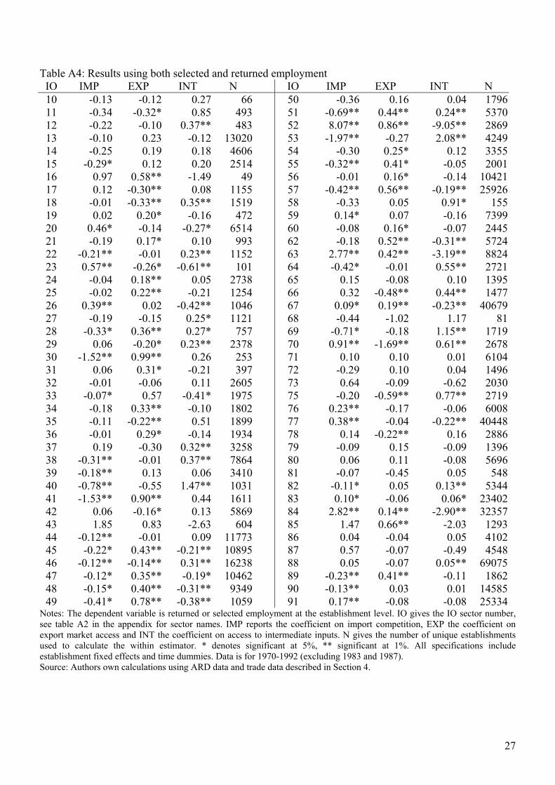
27

Table A4: Results using both selected and returned employment IO IMP EXP INT N IO IMP EXP INT N 10 -0.13 -0.12 0.27 66 50 -0.36 0.16 0.04 179611 -0.34 -0.32* 0.85 493 51 -0.69** 0.44** 0.24** 537012 -0.22 -0.10 0.37** 483 52 8.07** 0.86** -9.05** 286913 -0.10 0.23 -0.12 13020 53 -1.97** -0.27 2.08** 424914 -0.25 0.19 0.18 4606 54 -0.30 0.25* 0.12 335515 -0.29* 0.12 0.20 2514 55 -0.32** 0.41* -0.05 200116 0.97 0.58** -1.49 49 56 -0.01 0.16* -0.14 1042117 0.12 -0.30** 0.08 1155 57 -0.42** 0.56** -0.19** 2592618 -0.01 -0.33** 0.35** 1519 58 -0.33 0.05 0.91* 15519 0.02 0.20* -0.16 472 59 0.14* 0.07 -0.16 739920 0.46* -0.14 -0.27* 6514 60 -0.08 0.16* -0.07 244521 -0.19 0.17* 0.10 993 62 -0.18 0.52** -0.31** 572422 -0.21** -0.01 0.23** 1152 63 2.77** 0.42** -3.19** 882423 0.57** -0.26* -0.61** 101 64 -0.42* -0.01 0.55** 272124 -0.04 0.18** 0.05 2738 65 0.15 -0.08 0.10 139525 -0.02 0.22** -0.21 1254 66 0.32 -0.48** 0.44** 147726 0.39** 0.02 -0.42** 1046 67 0.09* 0.19** -0.23** 4067927 -0.19 -0.15 0.25* 1121 68 -0.44 -1.02 1.17 8128 -0.33* 0.36** 0.27* 757 69 -0.71* -0.18 1.15** 171929 0.06 -0.20* 0.23** 2378 70 0.91** -1.69** 0.61** 267830 -1.52** 0.99** 0.26 253 71 0.10 0.10 0.01 610431 0.06 0.31* -0.21 397 72 -0.29 0.10 0.04 149632 -0.01 -0.06 0.11 2605 73 0.64 -0.09 -0.62 203033 -0.07* 0.57 -0.41* 1975 75 -0.20 -0.59** 0.77** 271934 -0.18 0.33** -0.10 1802 76 0.23** -0.17 -0.06 600835 -0.11 -0.22** 0.51 1899 77 0.38** -0.04 -0.22** 4044836 -0.01 0.29* -0.14 1934 78 0.14 -0.22** 0.16 288637 0.19 -0.30 0.32** 3258 79 -0.09 0.15 -0.09 139638 -0.31** -0.01 0.37** 7864 80 0.06 0.11 -0.08 569639 -0.18** 0.13 0.06 3410 81 -0.07 -0.45 0.05 54840 -0.78** -0.55 1.47** 1031 82 -0.11* 0.05 0.13** 534441 -1.53** 0.90** 0.44 1611 83 0.10* -0.06 0.06* 2340242 0.06 -0.16* 0.13 5869 84 2.82** 0.14** -2.90** 3235743 1.85 0.83 -2.63 604 85 1.47 0.66** -2.03 129344 -0.12** -0.01 0.09 11773 86 0.04 -0.04 0.05 410245 -0.22* 0.43** -0.21** 10895 87 0.57 -0.07 -0.49 454846 -0.12** -0.14** 0.31** 16238 88 0.05 -0.07 0.05** 6907547 -0.12* 0.35** -0.19* 10462 89 -0.23** 0.41** -0.11 186248 -0.15* 0.40** -0.31** 9349 90 -0.13** 0.03 0.01 1458549 -0.41* 0.78** -0.38** 1059 91 0.17** -0.08 -0.08 25334

Notes: The dependent variable is returned or selected employment at the establishment level. IO gives the IO sector number, see table A2 in the appendix for sector names. IMP reports the coefficient on import competition, EXP the coefficient on export market access and INT the coefficient on access to intermediate inputs. N gives the number of unique establishments used to calculate the within estimator. * denotes significant at 5%, ** significant at 1%. All specifications include establishment fixed effects and time dummies. Data is for 1970-1992 (excluding 1983 and 1987). Source: Authors own calculations using ARD data and trade data described in Section 4.

28

Table A5: Results using distance decay ρ= 0.5 IO IMP EXP INT N IO IMP EXP INT N 10 -0.44 -1.25 1.46* 40 50 0.64 -0.76 0.78 21511 -1.51 -0.31 2.39 130 51 -1.44** 0.67** 0.77** 92612 -0.85 -0.09 0.80** 149 52 42.91** 3.91** -48.43** 22313 0.00 0.14 -0.16 1258 53 -1.78 0.56 0.99 30814 -3.02** 0.00 3.22** 1031 54 -1.57* 0.84** 1.18 52915 -0.13 0.60** -0.15 512 55 -0.56* 0.92* -0.30 25216 -10.24 0.74* 10.07 39 56 0.12 0.07 -0.02 74617 0.02 -0.43** 0.14 215 57 -1.42** 1.75** -0.51 82518 -0.19 -0.31 0.73** 375 58 -6.90* 4.38* 5.42** 5919 0.15 0.26 -0.15 121 59 0.26 -0.90** 0.67* 152920 -0.58 1.00** -0.23 798 60 -1.14 0.09 1.05 57921 0.35 0.21 -0.12 326 62 -0.18 0.40 -0.23 108322 -0.27 -0.12 0.69** 337 63 -0.19 0.68** -0.36 49223 1.70** -0.30 -2.15** 32 64 -1.95** 0.95 1.53** 32124 0.03 0.37** 0.26 609 65 0.07 -0.08 0.55* 34825 -0.27 0.28 0.16 290 66 1.17 -0.82 0.68* 13826 0.02 -0.16 0.00 161 67 -0.02 0.41** -0.36** 484027 -0.42 0.09 0.36 213 68 0.09 0.59 -1.05 5628 -1.04** 1.30** 1.08* 111 69 -3.89** -0.44 5.22** 71329 0.11 -1.06** 1.58** 422 70 1.30 -0.74 -1.05* 80830 -1.70** 0.64 0.15 75 71 1.01 -0.33 -0.08 103031 -0.06 0.25 -0.04 67 72 0.89 1.43 -3.26** 16632 0.19 -0.63* 0.68** 434 73 0.85 -1.11 -0.01 27533 0.80* 0.06 -0.31 673 75 -1.89** -0.79 2.27** 16534 0.09 0.57** -0.28* 751 76 0.22 -0.43 0.17 73335 0.73 -0.68* 0.45 418 77 0.52** -0.16 -0.59** 391836 0.31 0.57** -0.38 492 78 0.41* -0.48** 0.20 53537 0.23 1.05 -0.33 229 79 -0.54** 0.37 0.08 43738 -0.30 -0.66* 1.21** 628 80 -0.53** 0.65** 0.19 67939 -0.53** 0.00 0.56** 591 81 0.50 -0.50 -1.18 3140 -1.38** 1.11 1.11 97 82 -0.18 0.00 0.42** 135341 -4.05* 4.25** -1.15 244 83 -0.82** 0.76** 0.26** 165042 0.02 -0.33 0.23 877 84 6.22** 0.11 -6.30** 322043 0.16 -1.11 0.32 102 85 9.76** 1.33** -11.06** 32444 -0.36** -0.15 0.44* 2269 86 -2.16** 0.74** 1.54** 84345 -1.06** 1.73** -0.89** 1770 87 -1.86** 0.64** 1.20* 83046 -0.06 -0.23 0.48** 2347 88 0.22 -0.37** 0.04 497947 -0.62** 0.94** -0.19 1655 89 -0.22 0.33 0.05 53548 -0.53** 0.34 -0.23 941 90 -0.27* 0.04 0.00 215549 -1.02** 2.31** -0.46* 171 91 0.56* -0.65* 0.09 1323

Notes: The dependent variable is returned employment at the establishment level. IO gives the IO sector number, see table A2 in the appendix for sector names. IMP reports the coefficient on import competition, EXP the coefficient on export market access and INT the coefficient on access to intermediate inputs (all calculated with distance coefficient ρ=0.5). N gives the number of unique establishments used to calculate the within estimator. * denotes significant at 5%, ** significant at 1%. All specifications include establishment fixed effects and time dummies. Data is for 1970-1992 (excluding 1983 and 1987). Source: Authors own calculations using ARD data and trade data described in Section 4.

29

Table A6: Results using distance decay ρ= 1.5 IO IMP EXP INT N IO IMP EXP INT N 10 -0.10 -0.09 0.20 40 50 0.30 -0.21 0.01 21411 -0.99 -0.40 1.54* 129 51 -0.23 0.03 0.22** 92612 -0.16 0.00 0.17** 149 52 5.10** 0.56* -5.74** 22313 0.02 0.02 -0.05 1243 53 0.01 0.21 -0.25 30814 -0.16 0.14* 0.11 1027 54 -0.45* 0.14 0.40 52915 -0.13 0.10* 0.10 512 55 -0.15 0.31* -0.17 25216 3.52 0.18 -3.98 39 56 0.04 0.11 -0.13* 74117 0.06 -0.18** 0.02 215 57 -0.23** 0.35** -0.10 82218 -0.02 -0.10* 0.16** 372 58 1.40* -1.17* 0.70** 5919 0.05 0.04 -0.08 121 59 -0.03 -0.22** 0.22** 152820 -0.12 0.35** -0.19** 795 60 -0.20 0.04 0.17 57921 0.08 0.01 0.01 324 62 -0.05 0.12* -0.08* 108222 -0.06 -0.02 0.10* 335 63 -0.17 0.67** -0.51 49123 0.36** -0.10 -0.26* 30 64 -0.90** 0.30** 0.71** 31924 -0.16* 0.14** 0.12 608 65 0.14 -0.20 0.14* 34825 0.05 0.02 -0.04 289 66 0.09 -0.12 0.18** 13526 -0.04 0.01 0.01 161 67 0.09** 0.03 -0.11** 483227 -0.31 -0.04 0.28 212 68 -0.46 -0.26 0.74 5628 -0.46** 0.21* 0.39** 111 69 -0.89** -0.13 1.19** 71329 0.06 -0.10* 0.05 422 70 0.12 -0.16 -0.02 80830 -0.15 -0.04 0.09 75 71 -0.41 -0.28 0.79* 102931 -0.08 0.08 0.08 67 72 0.24 -0.56** 0.16 16632 -0.01 0.04 0.00 434 73 0.83** -0.15 -0.79** 27533 0.11 -0.02 0.01 669 75 -0.25 -0.30** 0.54** 16534 -0.12* 0.16* -0.01 751 76 0.03 0.10 -0.08* 73135 0.11 -0.08 0.11 418 77 0.07* 0.01 -0.09** 391436 0.09 0.02 -0.03 492 78 0.15* -0.01 -0.07 53437 -0.14 0.41* -0.14 229 79 -0.38* 0.13 0.17 43738 -0.03 0.08 0.00 627 80 -0.19* 0.12 0.16* 67939 -0.17** 0.02 0.16** 587 81 -0.15 -0.17 0.03 3140 -0.49** 0.41* 0.25 97 82 -0.07 0.07 0.05 135241 -0.70 0.58 0.07 244 83 -0.18** 0.23** 0.00 165042 -0.01 -0.02 0.03 877 84 0.67 0.02 -0.68 322043 0.22 -0.45 0.13 102 85 0.30 0.25** -0.53 32144 -0.09** -0.06 0.12** 2269 86 0.17 0.06 -0.20 83745 -0.10 0.29** -0.16** 1770 87 -0.08 0.07 0.01 82146 -0.03 -0.13** 0.18** 2342 88 -0.02 -0.01 -0.01 496447 -0.10* 0.17** -0.03 1655 89 -0.06 0.21** -0.12* 53548 -0.22** 0.17* -0.05 936 90 -0.08** 0.07 -0.05 215549 -0.19 0.69** -0.32** 171 91 0.16 -0.12 -0.05 1323

Notes: The dependent variable is returned employment at the establishment level. IO gives the IO sector number, see table A2 in the appendix for sector names. IMP reports the coefficient on import competition, EXP the coefficient on export market access and INT the coefficient on access to intermediate inputs (all calculated with distance coefficient ρ=1.5). N gives the number of unique establishments used to calculate the within estimator. * denotes significant at 5%, ** significant at 1%. All specifications include establishment fixed effects and time dummies. Data is for 1970-1992 (excluding 1983 and 1987). Source: Authors own calculations using ARD data and trade data described in Section 4.

30

Table A7: Intermediate access variable constructed ignoring own intermediates IO IMP EXP INT N IO IMP EXP INT N 10 -0.18 -0.25 0.41 40 50 0.27 -0.34 0.27 21511 -1.72* -0.45* 2.39** 130 51 -0.43** 0.28** 0.14* 92612 -0.27 -0.05 0.31** 149 52 15.78** 1.73** -17.83** 22313 0.05 0.00 -0.05 1258 53 0.43 0.37* -0.82 30814 -0.25** 0.07 0.30** 1030 54 -0.73** 0.26* 0.64 52915 -0.09 0.27* -0.04 512 55 -0.25* 0.32* -0.06 25216 -0.45* 0.55** -0.08 39 56 0.00 0.08 -0.02 74617 0.08 -0.25** 0.04 215 57 -0.51** 0.71** -0.21* 82518 -0.04 -0.19* 0.32** 375 58 0.03 -0.12 1.53** 5919 0.02 0.13 -0.08 121 59 0.20** -0.39** 0.19* 152920 -0.22 0.47** -0.18* 798 60 -0.11 0.05 0.06 57921 0.13 0.04 0.00 326 62 -0.08 0.16 -0.09 108322 -0.11 -0.07 0.26** 337 63 -0.58** 0.66** -0.09 49223 0.66** -0.19* -0.69** 32 64 -0.97** 0.35 0.84** 32124 -0.08 0.15** 0.14 609 65 0.08 -0.15 0.22* 34825 -0.02 0.10 -0.03 290 66 0.44* -0.42* 0.37** 13826 0.06 -0.07 -0.07 161 67 0.06 0.11* -0.16** 484027 -0.25 -0.03 0.21 213 68 -0.05 0.15 -0.21 5628 -0.50** 0.48** 0.38* 111 69 -0.46** -0.22 0.98** 71329 0.00 -0.24** 0.35** 422 70 0.44 -0.46 -0.15 80830 -0.59 0.18 0.13 75 71 0.28 -0.30 0.25 103031 -0.06 0.08 0.09 67 72 0.41 -0.53 -0.15 16632 0.04 -0.09 0.10 434 73 0.86* -0.50* -0.53 27533 0.36** -0.06 -0.09 673 75 -0.50* -0.44* 0.89** 16534 -0.09 0.25** -0.07 751 76 0.03 0.02 0.00 73335 0.17 -0.16* 0.27 418 77 0.12** 0.02 -0.17** 391836 -0.01 0.25* -0.06 492 78 0.22** -0.12* 0.02 53537 0.14 0.30 -0.08 229 79 -0.04 0.32* -0.25 43738 -0.02 -0.10 0.20 628 80 -0.24** 0.23* 0.17* 67939 -0.21** 0.06 0.16* 591 81 -0.17 -0.19 -0.15 3140 -0.68** 0.46 0.51 97 82 -0.04 -0.01 0.12** 135341 -1.81** 1.25** 0.28 244 83 -0.22** 0.26** 0.06 165042 0.01 -0.04 0.01 877 84 0.09** 0.06 -0.13** 322043 -0.27 -0.72 0.77 102 85 -0.23** 0.47** -0.19 32444 -0.09** -0.12 0.17** 2269 86 -0.55* 0.13* 0.47* 84345 -0.33** 0.62** -0.29** 1770 87 0.01 0.01 -0.06 83046 0.02 -0.22** 0.27** 2347 88 0.01 -0.06 0.00 497947 -0.26** 0.33** -0.02 1655 89 -0.04 0.21* -0.10 53548 -0.22** 0.07 0.00 941 90 -0.12** 0.05 -0.03 215549 -0.42* 1.04** -0.30** 171 91 0.26* -0.28* 0.02 1323

Notes: The dependent variable is returned employment at the establishment level. IO gives the IO sector number, see table A2 in the appendix for sector names. IMP reports the coefficient on import competition, EXP the coefficient on export market access and INT the coefficient on access to intermediate inputs. IMP and EXP constructed as for table 5. INT constructed ignoring own intermediates. N gives the number of unique establishments used to calculate the within estimator. * denotes significant at 5%, ** significant at 1%. All specifications include establishment fixed effects and time dummies. Data is for 1970-1992 (excluding 1983 and 1987). Source: Authors own calculations using ARD data and trade data described in Section 4.

31

Table A8: Robust errors IO IMP EXP INT N IO IMP EXP INT N 10 -0.18 -0.25 0.41 39 50 0.26 -0.33 0.27 14211 -1.81* -0.45 2.47* 114 51 -0.54** 0.25 0.29* 64012 -0.27 -0.05 0.31** 119 52 17.43** 1.72** -19.47** 14613 0.07 0.01 -0.08 865 53 1.16 0.48* -1.66* 19414 -0.66 0.13 0.66 769 54 -0.73 0.27 0.63 39315 -0.16 0.23* 0.09 390 55 -0.27* 0.38 -0.10 19816 -3.59 0.67** 3.06 18 56 0.01 0.07 -0.01 52617 0.08 -0.25** 0.03 175 57 -0.53** 0.70** -0.16 53418 -0.02 -0.20* 0.33** 307 58 -0.09 -0.12 1.61** 4219 0.04 0.13 -0.10 92 59 0.06 -0.42** 0.35* 116820 -0.17 0.48** -0.24 571 60 -0.40 0.05 0.35 43521 0.18 0.06 -0.08 254 62 -0.06 0.13 -0.07 82022 -0.11 -0.07 0.27** 288 63 -0.23 0.63** -0.37 37623 0.66** -0.19 -0.69** 25 64 -0.82** 0.29 0.73** 24424 -0.09 0.19* 0.13 482 65 0.08 -0.15 0.23* 27925 -0.09 0.03 0.17 204 66 0.44 -0.42 0.37** 10626 0.06 -0.06 -0.08 123 67 0.07 0.11 -0.16** 357627 -0.26 -0.03 0.23 169 68 -0.03 0.16 -0.24 4228 -0.50** 0.49** 0.38 87 69 -1.50** -0.23 2.02** 52229 -0.04 -0.25* 0.39** 294 70 0.39 -0.39 -0.15 63630 -0.67 0.20 0.17 65 71 0.31 -0.32 0.26 78731 0.04 0.18 0.04 60 72 0.41 -0.53 -0.15 12732 0.02 -0.04 0.09 334 73 0.86 -0.50* -0.53 19333 0.36* -0.06 -0.09 553 75 -0.62* -0.44 1.00** 12834 -0.07 0.25** -0.09 614 76 0.02 0.02 0.01 53335 0.03 -0.18 0.44 299 77 0.13* 0.02 -0.18** 277136 0.11 0.25* -0.18 398 78 0.22* -0.12 0.02 40037 -0.11 0.35 -0.02 159 79 -0.04 0.35 -0.26 34638 -0.05 -0.09 0.23 430 80 -0.26 0.28 0.11 48239 -0.20** 0.06 0.16 466 81 -0.17 -0.18 -0.16 2140 -0.69** 0.46 0.52 65 82 -0.05 0.00 0.13* 102841 -1.76 1.31** 0.17 190 83 -0.22* 0.25* 0.06 118342 0.01 -0.05 -0.01 651 84 1.86** 0.06 -1.89** 206643 -0.44 -0.76 0.98 68 85 1.55* 0.47** -1.96* 26044 -0.13** -0.10 0.21* 1669 86 -0.67* 0.16* 0.57* 68345 -0.31* 0.61** -0.30** 1279 87 0.05 -0.01 -0.09 66946 -0.02 -0.20* 0.28** 1669 88 -0.01 -0.05 0.00 312947 -0.23** 0.36** -0.07 1212 89 -0.03 0.20 -0.08 42648 -0.22* 0.10 -0.04 696 90 -0.15* 0.06 -0.02 153549 -0.42* 1.04** -0.30* 129 91 0.23* -0.22 -0.02 964

Notes: The dependent variable is returned employment at the establishment level. IO gives the IO sector number, see table A2 in the appendix for sector names. IMP reports the coefficient on import competition, EXP the coefficient on export market access and INT the coefficient on access to intermediate inputs. N gives the number of unique establishments used to calculate the within estimator. Standard errors are robust to arbitrary heteroscedasticity. * denotes significant at 5%, ** significant at 1%. All specifications include establishment fixed effects and time dummies. Data is for 1970-1992 (excluding 1983 and 1987). Source: Authors own calculations using ARD data and trade data described in Section 4.

32

Table A9: Clustered robust errors IO IMP EXP INT N IO IMP EXP INT N 10 50 0.26 -0.33 0.27 14211 -1.81 -0.45 2.47 114 51 -0.54 0.25 0.29 64012 -0.27 -0.05 0.31 119 52 17.43* 1.72** -19.47* 14613 0.07 0.01 -0.08 865 53 1.16 0.48* -1.66 19414 -0.66 0.13 0.66 769 54 -0.73 0.27 0.63 39315 -0.16 0.23 0.09 390 55 -0.27 0.38 -0.10 19816 56 0.01 0.07 -0.01 52617 0.08 -0.25* 0.03 175 57 -0.53** 0.70** -0.16 53418 -0.02 -0.20 0.33 307 58 -0.09 -0.12 1.61** 4219 0.04 0.13 -0.10 92 59 0.06 -0.42* 0.35 116820 -0.17 0.48* -0.24 571 60 -0.40 0.05 0.35 43521 0.18 0.06 -0.08 254 62 -0.06 0.13 -0.07 82022 -0.11 -0.07 0.27 288 63 -0.23 0.63** -0.37 37623 64 -0.82 0.29 0.73* 24424 -0.09 0.19 0.13 482 65 0.08 -0.15 0.23 27925 -0.09 0.03 0.17 204 66 0.44 -0.42 0.37* 10626 0.06 -0.06 -0.08 123 67 0.07 0.11 -0.16* 357627 -0.26 -0.03 0.23 169 68 -0.03 0.16 -0.24 4228 -0.50 0.49 0.38 87 69 -1.50* -0.23 2.02** 52229 -0.04 -0.25 0.39 294 70 0.39 -0.39 -0.15 63630 -0.67 0.20 0.17 65 71 0.31 -0.32 0.26 78731 0.04 0.18 0.04 60 72 0.41 -0.53 -0.15 12732 0.02 -0.04 0.09 334 73 0.86 -0.50 -0.53 19333 0.36 -0.06 -0.09 553 75 -0.62 -0.44 1.00** 12834 -0.07 0.25 -0.09 614 76 0.02 0.02 0.01 53335 0.03 -0.18 0.44 299 77 0.13 0.02 -0.18* 277136 0.11 0.25 -0.18 398 78 0.22 -0.12 0.02 40037 -0.11 0.35 -0.02 159 79 -0.04 0.35 -0.26 34638 -0.05 -0.09 0.23 430 80 -0.26 0.28 0.11 48239 -0.20 0.06 0.16 466 81 40 -0.69** 0.46 0.52 65 82 -0.05 0.00 0.13 102841 -1.76 1.31 0.17 190 83 -0.22 0.25 0.06 118342 0.01 -0.05 -0.01 651 84 1.86 0.06 -1.89 206643 -0.44 -0.76 0.98 68 85 1.55 0.47 -1.96 26044 -0.13 -0.10 0.21 1669 86 -0.67 0.16 0.57 68345 -0.31 0.61* -0.30 1279 87 0.05 -0.01 -0.09 66946 -0.02 -0.20* 0.28** 1669 88 -0.01 -0.05 0.00 312947 -0.23 0.36* -0.07 1212 89 -0.03 0.20 -0.08 42648 -0.22 0.10 -0.04 696 90 -0.15 0.06 -0.02 153549 -0.42 1.04** -0.30 129 91 0.23 -0.22 -0.02 964

Notes: The dependent variable is returned employment at the establishment level. IO gives the IO sector number, see table A2 in the appendix for sector names. IMP reports the coefficient on import competition, EXP the coefficient on export market access and INT the coefficient on access to intermediate inputs. N gives the number of unique establishments used to calculate the within estimator. Standard errors are robust to arbitrary heteroscedasticity and allow for arbitrary within TTWA correlation. * denotes significant at 5%, ** significant at 1%. All specifications include establishment fixed effects and time dummies. Data is for 1970-1992 (excluding 1983 and 1987). Source: Authors own calculations using ARD data and trade data described in Section 4.

33

Table A10: First difference estimator IO IMP EXP INT N IO IMP EXP INT N 10 0.51 -0.76 0.25 39 50 -0.08 0.04 0.10 14211 -4.70 -3.47 7.20 114 51 -0.29* 0.23 0.10 64012 -0.05 0.04 0.05 119 52 6.26* 0.02 -6.44* 14613 -0.07 0.26* -0.16 865 53 1.28 0.08 -1.24 19414 -0.66 -0.04 0.69 769 54 0.40 0.08 -0.49 39315 0.10 0.11 -0.32 390 55 -0.11 0.48 -0.44 19816 -1.35 0.11 1.24 18 56 -0.08 0.57** -0.60** 52617 0.27 -0.24* -0.02 175 57 -0.14 0.09 0.10 53418 -0.10 0.12 0.04 307 58 -0.03 -0.20 0.76 4219 -0.07 0.11 0.00 92 59 0.23** 0.24* -0.48** 116820 -0.22 0.12 0.11 571 60 -0.67* -0.06 0.73* 43521 0.23 -0.12 -0.03 254 62 0.01 -0.03 0.05 82022 -0.47** 0.06 0.26** 288 63 -0.44 1.24 -0.84 37623 0.15 -0.12 -0.02 25 64 -0.11 0.38 -0.04 24424 -0.49** 0.30** 0.27** 482 65 -0.05 -0.24 0.31 27925 0.14 -0.19 0.07 204 66 1.83 -2.01 0.89 10626 -0.02 0.15 -0.16 123 67 0.07 -0.05 0.06 357627 -0.88* -0.40** 0.97* 169 68 0.98 1.64 -2.75 4228 -0.37 -0.01 0.28 87 69 -0.54 -0.02 0.67 52229 -0.19 0.21 -0.06 294 70 0.06 0.04 -0.06 63630 -0.30 -0.18 0.29 65 71 -0.30 -0.96* 1.09 78731 -0.85 -0.19 0.88 60 72 0.76 -0.29 -0.43 12732 -0.13* 0.22 -0.14 334 73 -1.56** 0.52 0.77** 19333 -0.03 0.29 -0.19 553 75 0.04 -0.06 0.05 12834 -0.15* 0.19** -0.06 614 76 -0.43 0.34 0.07 53335 1.02 -0.27 -0.61 299 77 0.08 -0.08 0.01 277136 0.53 -0.70 0.07 398 78 0.06 0.28 -0.31 40037 -0.03 -0.06 0.16 159 79 -0.44 1.29 -0.87 34638 0.01 -0.11 0.07 430 80 -0.26 0.31 -0.03 48239 -0.03 0.02 -0.01 466 81 -1.43 -1.33 2.70 2140 -0.07 -0.13 0.22 65 82 0.03 -0.07 0.06 102841 0.51 0.30 -0.92 190 83 -0.08 0.10 -0.04 118342 0.00 -0.11 0.07 651 84 0.10 0.02 -0.09 206643 2.12 0.89 -2.98 68 85 -0.85 -0.23 1.10 26044 0.03 -0.06 0.01 1669 86 -0.52 0.04 0.50 68345 -0.09 0.21 -0.18 1279 87 0.44 -0.11 -0.34 66946 0.00 0.03 -0.05 1669 88 -0.01 0.00 -0.01 312947 -0.06 0.14* -0.07 1212 89 0.10 -0.02 -0.02 42648 -0.04 -0.05 0.11 696 90 0.03 -0.09 0.07 153549 -0.46** 0.57* -0.10 129 91 0.44** -0.52* 0.16 964

Notes: The dependent variable is returned employment at the establishment level. IO gives the IO sector number, see table A2 in the appendix for sector names. IMP reports the coefficient on import competition, EXP the coefficient on export market access and INT the coefficient on access to intermediate inputs. N gives the number of unique establishments used to calculate the first difference estimator. * denotes significant at 5%, ** significant at 1%. All specifications include establishment fixed effects and time dummies. Data is for 1970-1992 (excluding 1983 and 1987). Source: Authors own calculations using ARD data and trade data described in Section 4.

34

Table A11: Long differences IO IMP EXP INT N IO IMP EXP INT N 10 -0.11 0.78 -0.21 18 50 -0.22 -0.54 0.96* 3011 -0.19 -0.05 1.01 41 51 0.00 0.08 0.02 14412 0.02 -0.21 0.14 40 52 -2.07 2.53 -0.99 1613 0.03 0.06 -0.07 204 53 0.64 1.36 -2.00 1514 -0.11 0.11 0.14 142 54 0.01 -0.10 0.21 10115 -1.11* 0.41 0.97 117 55 0.08 -0.05 0.20 5716 56 0.08 -0.04 0.02 10617 0.03 -0.10 -0.18 73 57 -0.13 0.03 0.33 9818 0.16 -0.08 0.26 97 58 -0.81 0.85 0.69 1319 -0.14 0.10 0.18 24 59 -0.06 -0.08 0.12 30320 -0.06 -0.03 0.17 134 60 -0.33 0.25 0.14 14121 0.26 0.05 -0.18 70 62 -0.08 0.04 0.07 19222 -0.04 0.07 0.18 126 63 0.11 -0.04 -0.09 10423 64 -0.47 0.29 0.38 5824 -0.02 0.03 0.27 160 65 0.23 -0.18 0.18 10125 0.01 0.45 -0.31 64 66 0.25 -0.50 0.63* 3226 -0.06 -0.11 -0.02 35 67 0.02 -0.01 0.03 79827 -0.24 0.36 -0.20 63 28 -1.07** 1.39** 0.18 31 69 -0.07 0.53 -0.15 11429 0.14 -0.29 0.44 76 70 -0.56 0.80 -0.57 18130 -0.39 0.53 -0.10 24 71 0.07 0.22 0.11 21131 0.39 0.45 -0.28 17 72 0.85 0.43 -1.49* 3532 -0.02 -0.02 0.14 99 73 0.30 -0.42 -0.33 3833 0.46 -0.44 0.06 137 75 -0.15 -0.32 0.60* 3234 0.11 -0.10 0.14 179 76 0.56** -0.43 -0.32** 13935 -0.01 -0.03 0.15 90 77 0.02 0.04 -0.02 54136 -0.07 0.08 0.12 111 78 0.33 0.00 -0.22 15137 -0.91 1.09 0.02 29 79 -0.61* 0.77** 0.21 8138 0.46 -0.47 -0.03 107 80 -1.31** 1.22** 0.10 14839 -0.20 0.06 0.17 166 81 0.26 -0.84 -0.50 1140 -0.95* 1.69** -0.30 18 82 -0.72* 0.72* 0.03 23641 -1.06 1.25 -0.21 39 83 -0.16 0.15 0.24* 25742 0.15 -0.08 -0.17 164 84 -0.04 -0.04 0.16 51743 0.30 0.27 -1.06 15 85 0.40** -0.29 -0.25 9544 -0.25** 0.21* 0.03 411 86 0.03 -0.08 0.07 26245 -0.24** 0.30** 0.06 255 87 -0.03 -0.06 0.02 21046 -0.08 0.13 -0.03 311 88 0.04 -0.10 -0.01 89047 -0.13 0.08 0.16 306 89 0.16 0.07 -0.02 13548 -0.08 0.15 -0.19 171 90 -0.05 -0.05 0.00 33049 -0.54 1.16* -0.17 32 91 -0.07 -0.06 0.04 216

Notes: The dependent variable is returned or selected employment at the establishment level. IO gives the IO sector number, see table A2 in the appendix for sector names. IMP reports the coefficient on import competition, EXP the coefficient on export market access and INT the coefficient on access to intermediate inputs. N gives the number of unique establishments used to calculate the long difference estimator (long differences are the based on average employment 1984-1986 minus average employment 1970-1972). * denotes significant at 5%, ** significant at 1%. All specifications include establishment fixed effects and time dummies. Data is for 1970-1992 (excluding 1983 and 1987). Source: Authors own calculations using ARD data and trade data described in Section 4.

CENTRE FOR ECONOMIC PERFORMANCE Recent Discussion Papers

587 Pierre-Philippe Combes

Henry G. Overman The Spatial Distribution of Economic Activities in the European Union

586 Henry G. Overman Can We Learn Anything from Economic Geography Proper?

585 A. B. Bernard J. Bradford Jensen P. K. Schott

Falling Trade Costs, Heterogeneous Firms and Industry Dynamics

584 A. B. Bernard J. Bradford Jensen P. K. Schott

Survival of the Best Fit: Exposure to Low-Wage Countries and the (Uneven) Growth of U.S. Manufacturing Plants

583 S. Wood S. Moore

Reviewing the Statutory Union Recognition (ERA 1999)

582 T. Kirchmaier Corporate Restructuring and Firm Performance of British and German Non-Financial Firms

581 C. Dougherty Why Is the Rate of Return to Schooling Higher for Women than for Men?

580 S. Burgess D. Mawson

Aggregate Growth and the Efficiency of Labour Reallocation

579 S. Nickell Poverty and Worklessness in Britain

578 D. Marsden Renegotiating Performance: the Role of Performance Pay in Renegotiating the Effort Bargain

577 S. Nickell A Picture of European Unemployment: Success and Failure

576 A. de Coulon M. Piracha

Self-Selection and the Performance of Return Migrants: the Source Country Perspective

575 H. Steedman K. Wagner J. Foreman

The Impact on Firms of ICT Skill-Supply Strategies: An Anglo-German Comparison

574 S. Gibbons The Costs of Urban Property Crime

573 R. Griffith S. Redding H. Simpson

Productivity Convergence and Foreign Ownership at the Establishment Level

572 S. Redding P. K. Schott

Distance, Skill Deepening and Development: Will Peripheral Countries Ever Get Rich?

571 B. Petrongolo C. A. Pissarides

Scale Effects in Markets with Search

570 M. Coles B. Petrongolo

A Test Between Unemployment Theories Using Matching Data

569 A. Bryson L. Cappellari C. Lucifora

Does Union Membership Really Reduce Job Satisfaction?

568 A. Bryson R. Gomez

Segmentation, Switching Costs and the Demand for Unionization in Britain

567 M. Gutiérrez-Domènech Employment After Motherhood: A European Comparison

566 T. Kirchmaier The Performance Effects of European Demergers

565 P. Lopez-Garcia Labour Market Performance and Start-Up Costs: OECD Evidence

564 A. Manning The Real Thin Theory: Monopsony in Modern Labour Markets

563 D. Quah Digital Goods and the New Economy

562 H. Gospel P. Willman

High Performance Workplaces: the Role of Employee Involvement in a Modern Economy. Evidence on the EU Directive Establishing a General Framework for Informing and Consulting Employees

561 L. R. Ngai Barriers and the Transition to Modern Growth

To order a discussion paper, please contact the Publications Unit

Tel 020 7955 7673 Fax 020 7955 7595 Email info@cep.lse.ac.uk Web site http://cep.lse.ac.uk