The Impact of Divorce Laws onMarriage

Imran Rasul∗

University of Chicago and CEPR†

February 2003

Abstract

Marriage rates have declined dramatically over the last 30 years. Thispaper studies to what extent divorce laws have changed incentives to marry.Using US state level panel data I provide evidence that after the adoptionof unilateral divorce, marriage rates declined significantly and permanently inadopting states. This decline accounts for half of the initial gap in marriagerates between adopting and non-adopting states. The effect of unilateral divorcelaw is greatest for marriage rates amongst younger age cohorts, those marryingfor the first time, and whites. The duration of marriages that take place underunilateral divorce is also found to be significantly greater than those that occurunder mutual consent. Taken together the results suggest unilateral divorcelaw reduces incentives to marry, but those couples that do marry are bettermatched than under mutual consent. This is argued to be consistent with amodel of search in marriage markets, where individuals learn the true gains ofmarriage over divorce before and during marriage.

Keywords: Marriage, Unilateral Divorce.

JEL Classification: J12, K19.

∗I thank Tim Besley and Robin Burgess for comments on an earlier draft. I have also benefitedfrom discussions with Oriana Bandiera, Wouter Dessein, Jonathan Guryan, and seminar participantsat Chicago. I am grateful to Justin Wolfers and Tanvi Desai for providing some of the data used.All errors are my own.

†Address for correspondence: Walker 415, University of Chicago Graduate School of Business,1101 East 58th Street, Chicago IL 60637, USA. Tel: 1-773-834-8690; Fax: 1-773-702-0458; E-mail:imran.rasul@gsb.uchicago.edu.

1

1 Introduction

The family is a building block of society that has changed dramatically over thepast two generations. Most attention has been on the rise in divorce. In particular,whether there exists a causal relation between divorce laws and the rise in divorcerates. Ironically much of this debate has taken place when divorce rates have beenfalling. Indeed the last 15 years has been the longest period of sustained decline indivorce in America since records began in 1860.1

Of more concern now is the sustained decline in marriage. Today, fewer people aremarrying than at any time in the past 40 years, the children of the unmarried accountfor nearly as many as those living in single parent households, and the majority ofbirths occur out of wedlock.2

The decline in marriage is of concern if we believe marriage to be a good thing,in that there are positive private and social returns to marriage. A large body ofliterature, summarized in Waite and Gallagher (2000), shows a strong correlation be-tween being married and having better health, higher wages, and accumulating morewealth. They argue these effects exist for married individuals relative to cohabiteesas well as divorced individuals.Furthermore, changing marital patterns have implications for the life cycle behav-

ior of individuals - their attachment to the labor market, savings, and fertility. Evenignoring the welfare consequences of those directly involved, the decline in marriagehas far reaching macroeconomic consequences.This paper studies the effects of divorce laws on incentives to marry. In particular

I consider the effects on marriage rates of two changes in divorce law - (i) from mutualconsent to unilateral divorce; (ii) from fault based to no-fault divorce. In much of theearlier literature these laws have been referred to almost interchangeably. Howevereconomic theory would suggest they ought to have very different effects on incentivesto marry.Unilateral divorce re-assigns the right to divorce. In contrast, no-fault divorce

reduces the costs of exiting marriage.3

If spouses can bargain efficiently, the Coasean theorem implies that moving frommutual consent to unilateral divorce only affects the distribution of welfare withinmarriage, not the incidence of marriage and divorce. However spouses may be unableto bargain efficiently because they cannot commit ex ante to all possible divisions ofthe gains from marriage, or because the benefits from household public goods such aschildren are neither divisible nor transferable. In this case the incidence of marriage

1This paper focuses exclusively on the United States. Similar trends in marriage and divorce areobserved in the UK and Canada, both of which have reformed divorce laws as in the United States.

2In 1994 37% of children in single parent households were living with divorced parents, 36% wereliving with a never married parent, and the remainder lived with a separated parent (Bureau of theCensus (1996)). The percentage of births to unmarried women rose from 5% in 1940 to 65% in 2000(National Vital Statistics Report (2000)).

3Jacob (1988) also argues that unilateral divorce has no relation to the cost of divorce.

2

and divorce would be different under mutual consent and unilateral divorce regimes.To make precise the effects of both laws, I proceed in two stages. I first set out

a model of search in marriage markets, where individuals learn the true gains frommarriage over divorce before and during marriage. I then test the predictions of thetheory using US state level panel data on marriage rates over the period 1960-2000.The search model makes precise that when spouses are unable to bargain effi-

ciently, moving from mutual consent to unilateral divorce has two effects which workin opposite directions - (i) the probability of divorce for any given couple rises, reduc-ing the value of marrying today; (ii) each spouse is guaranteed at least their payoff indivorce if the marriage continues, and so cannot be locked into a bad marriage. Thisincreases the value of marrying today.If the first order effect of unilateral divorce is to increase the probability of divorce,

individuals are only willing to enter matches of potentially higher quality than undermutual consent divorce. This increases the average quality of matched couples.In this case, unilateral divorce causes individuals to become more selective in

the marriage market, the flow of singles into marriage decreases, but because theprobability of divorce rises, the stock of singles increases. Hence the change in thesteady state marriage rate is ambiguous. Similarly the effect on the divorce rateis ambiguous because although the flow of individuals from marriage into divorceincreases, the stock of married individuals falls.If the first order effect of unilateral divorce is to ensure spouses cannot be locked

into a bad marriage, individuals are willing to enter matches of potentially lowerquality than under mutual consent divorce. This worsens the average quality ofmatched couples as individuals are less selective in the marriage market. The effectson the marriage market then work in the opposite direction.Which of these two channels is more important cannot be determined a priori. It

is left to the empirical analysis to distinguish the dominant effect.Moving from fault based to no-fault divorce lowers the costs of exiting marriage.

Divorce costs are lower under no-fault because less proof is required to file for divorce,and courts cannot impose financial penalties on at-fault spouses. By reducing thecosts of exiting marriage, no-fault divorce raises spouse’s divorce payoffs, and increasesthe lifetime value of marrying today. This is because the lower expected gains frommarriage are more than offset by the higher divorce payoff.Under no-fault divorce individuals are willing to enter a match of potentially lower

quality than under fault based divorce, precisely because the cost of exiting marriagehas fallen. This increases the marriage rate, worsens the average quality of matchedcouples, and subsequently leads to a higher steady state divorce rate.4

4Models of search in marriage markets borrow heavily from the labor literature. No-fault divorceis similar to reducing firing costs. The fact that this has an effect on match formation is wellestablished in the labor literature. However, the move from mutual consent to unilateral divorce isnot so easily translatable into the labor literature. This is particularly so because families, unlikeworkers and firms, may not be able to bargain efficiently. Furthermore, assortive matching in

3

The model thus makes clear that each law has different effects on marital forma-tion, marital dissolution, and selection into marriage.The main empirical results are as follows. First, before the introduction of uni-

lateral divorce, marriage rates were 20% higher in states that eventually adopted.Marriage rates declined significantly in states that adopted unilateral divorce. Thedecline in marriage caused by unilateral divorce is present a decade after the imple-mentation of unilateral divorce and accounts for half of the initial gap in marriagerates between adopting and non-adopting states. The effects are greatest in marriagesinvolving younger age cohorts, whites, and those marrying for the first time.The result that unilateral divorce caused a decline in marriage, is consistent with

the probability of any given couple divorcing having risen and more than offsettingthe effect that individuals cannot be locked into a bad marriage.Second, the composition of those marrying under unilateral divorce differed from

earlier marriage cohorts. In particular, the difference-in-difference in the durationof marriages that take place under unilateral divorce rather than mutual consent,increases significantly. This suggests unilateral divorce causes better selection intomarriage.Throughout I find little evidence that no-fault divorce affected marriage rates.

Taken together, the results suggest the first order effect of changes in divorce laws onmarriage has been through changes in the right to divorce, rather than the costs ofexiting marriage.This paper makes three contributions to the literature. First, the theoretical

analysis makes clear the effects of divorce law on selection into marriage, maritalformation, marital dissolution, and the relation between the two.Second the paper provides new evidence on some of the unintended consequences

of divorce law reforms.5 Unilateral divorce accounts for much of the decline in mar-riage especially amongst younger cohorts. This result is robust to the inclusion ofother laws such as legalized abortion, and other observable determinants of marriagerates.Third, the paper helps explain earlier findings in the literature on the relation

between divorce laws and divorce rates (Friedberg (1998), Gruber (2000), Wolfers(2000)). By not explicitly taking account of the (perhaps unintended) effects of di-vorce laws on incentives to marry and selection into marriage, least squares estimatesof the impact of divorce laws on divorce rates are likely to be underestimated.The paper is organized as follows. Section two provides an overview of changes

in divorce law that swept through America in the 1970s. Section three presents amodel of search and learning in marriage markets. Section four contains the empirical

marriage markets is perhaps more prevalent than in the labor market (Burdett and Coles (1997)).5Brinig and Crafton (1994) regress state level marriage rates (defined as the number of marriages

per 1000 of the population) from 1965-87 on a time trend, state adult population and a dummy forunilateral divorce (which they refer to as no-fault) but do not include state fixed effects. They finda significantly negative effect of unilateral divorce on marriage rates.

4

analysis. Section five concludes. Proofs and data definitions are in the appendices.

2 A Brief History of Divorce Law

The 1970s witnessed major changes in divorce laws. Foremost of these was the intro-duction of unilateral divorce. Between 1968 and 1977 the majority of states passedsuch laws, moving from a regime in which the dissolution of marriage required themutual consent of both spouses, to one in which spouses could unilaterally file fordivorce.To understand the motivation behind such laws, it is instructive to consider the

case of California, one of the earliest adopters.6 Criticism of the mutual consent sys-tem stemmed from the view that it reduced the welfare of spouses, and led to perjuredtestimony in collusive divorce proceedings that fostered disrespect towards the law.7

Californian legislators believed they would improve welfare within families and endthe legal convention in which extreme cruelty was almost the only universal groundfor divorce (Parkman (1992)). The Californian Family Law Act became effective in1970 and established two grounds on which spouses could unilaterally file for divorce- (i) irreconcilable differences; (ii) incurable insanity.The reform received widespread support from conservative sections of society who

perceived it as strengthening families and reducing the opportunities for divorce.Lobbies for divorced men and feminist groups also supported the move. Male lobbygroups perceived mutual consent divorce to work in favor of wives because men hadto “bribe” their wives for them to agree to divorce. Feminist lobbies viewed thereform as eliminating an unjust element of the legal system because women wereoften unable to “bribe” their husbands to divorce. Little if any consideration wasgiven to the effect on the incentives to marry.In addition to changing the right to divorce, the Californian law also established

that the assignment of fault did not have to be established in divorce cases, nor didfault play any role in divorce settlements. Figure 1 shows the rapid spread of bothunilateral and no-fault divorce laws. Table 1 gives the years in which the laws werepassed by state.This second strand of California’s law change, no-fault divorce, has often been

confused with unilateral divorce. The innovative part of the Californian legislation

6The Californian experience is important because the National Conference on Commissioners ofUniform State Laws later based the standard for marital dissolution in the Uniform Marriage andDivorce Act (1974) on California’s requirements for divorce.

7Both problems stem from whether spouses bargain efficiently. If spouses were unable or unwillingto make such agreements, the marriage could not be dissolved under mutual consent even thoughit would be Pareto efficient to do so. If spouses could bargain efficiently, the perception was thatmen had to “bribe” their wives in order for them to consent to divorce leading to collusion betweenspouses in court proceedings. Ellman et al (1998) provide evidence on how perjured testimony andcollusion between spouses, were commonplace in divorce cases under mutual consent.

5

was the introduction of unilateral divorce. As Gruber (2000) notes, in 1960 some20% of the population already resided in no-fault states. Distinguishing unilateralfrom no-fault divorce is important because each law has potentially different effectson incentives to marry.The next section makes clear that when spouses are unable to bargain efficiently,

moving from mutual consent to unilateral divorce has two effects - (i) it increases theprobability of divorce for any given couple, reducing the expected lifetime value ofmarrying today; (ii) it guarantees each spouse at least their divorce payoff in marriage,so that they cannot be locked into a bad marriage, and this increases the expectedlifetime value of marrying today.If the first order effect of unilateral divorce is to increase the probability of divorce,

individuals are only willing to enter matches of potentially higher quality than undermutual consent divorce. This can cause the marriage rate to fall. As the averagequality of matched couples increases, in the long run this can cause the divorce rateto fall.In contrast, moving from fault based to no-fault divorce lowers the costs of exiting

marriage. Individuals are willing to enter a match of potentially lower quality thanunder fault based divorce, precisely because it is easier to leave any marriage. Thisincreases the marriage rate, worsens the average quality of matched couples, andsubsequently leads to a higher steady state divorce rate.

3 A Basic Framework

The marriage market is modelled in discrete time with finitely lived risk neutralparticipants.8 Each period new individuals are born into the marriage market at rate1 − β, and the same fraction of individuals die each period. Birth and death ratesare the same across men and women, so total population remains constant and isnormalized to one, with an equal number of men and women. An individual can bein one of three marital states - married, divorced or single (i.e. never married). Thetiming of the marriage market is as follows;

1. each period every surviving individual matches with a person of the oppositesex with certainty. The matched couple receive an imperfect signal (σ) of the gainfrom their potential marriage.2. each individual decides to marry or remain single. If at least one of the matched

couple decides to remain single, both re-enter the marriage market.3. if they marry, the actual gain from marriage (φ) is realized in the next period.

The couple can then either remain married forever or divorce and remain divorcedforever.

8I extend the model in Bougheas and Georgellis (1999) to take account of remarriage, derivesteady state marriage and divorce rates, and consider the effect of unilateral divorce.

6

This framework emphasizes the role of learning in marriage markets. There aretwo stages of learning - first, when individuals meet in the marriage market they learnsomething but not everything about each other, embodied in the sig-nal, σ. The signal can be thought of as being related to the immediately observabletraits of a potential marriage partner.9 The signal determines whether an individualis better off marrying today or remaining single.The second stage of learning takes place within marriage. Married individuals up-

date their prior beliefs about the gains from marriage (φ) by accumulating knowledgeduring marriage. This determines whether the individual is better off remaining mar-ried or divorcing.10 Divorce is thus an optimal response to new information receivedduring marriage.Individuals do not remarry and all participants are ex ante identical. I relax both

of these assumptions later.The signal of the gains frommarriage takes a realization in the closed set [σ, ..., σ] =

Σ. The probability density function of signals is f(σ), assumed everywhere positive,with associated cumulative density F (σ). Conditional on the signal, the actual gainfrom marriage is φ with probability g(φ|σ). The distribution g(φ|σ) is assumed uni-modal and symmetric with support

£φ, φ

¤for all signals. The associated cumulative

distribution is G(φ|σ).I assume signals are ordered such that the distribution of the gains from marriage

generated by higher signals stochastically dominate the distributions given by lowersignals;

Assumption 1 (Stochastic Dominance): Gσ(φ|σ) < 0 for all φ.Higher signals therefore imply higher expected gains from marriage. Married

individuals are better off remaining married if the payoff in marriage is higher thanthe divorce payoff each period. The per period payoff to remaining married is φ, theper period divorce payoff is exogenously given by φ∗.11

Hence the expected lifetime value of marrying today having received signal σ in

9These traits relate to market outcomes, such as earnings capacity, as well as non-market out-comes, such as personality.10In the labor literature, search models emphasize both “on-the-job” search, where separation

occurs as workers re-evaluate the value of the current match as information about alternative matchesbecomes available (extensive search); and learning about job characteristics (intensive search), whereseparation occurs as workers learn the true quality of the match. Previous models of search inmarriage markets include Becker et al (1977) and Mortensen (1988)). As in Bougheas and Georgellis(1999) and Brien et al (2002), this model focuses on learning before and within marriage. Allowingfor on-the-job search gives qualitatively similar results if the cost of searching on-the job is sufficientlyhigher than the cost of search for singles.11The results are robust to the divorce payoff being stochastic as long as its expected value is

independent of the signal σ.

7

the marriage market is;

V (M |σ) =Z φ

φ

φg(φ|σ)dφ+ β

1− β

"Z φ

φ∗φg(φ|σ)dφ+G(φ∗|σ)φ∗

#(1)

where β is the probability the individual survives into the next period. The first termis the expected marriage payoff in the first period of marriage, conditional on havingreceived signal σ. The first term in brackets is the expected payoff in marriage fromthe second period of marriage onwards, conditional on the marriage remaining intact,namely if φ ≥ φ∗. The second term in brackets is the expected divorce payoff whereG(φ∗|σ) is the conditional probability of the couple divorcing.If the individual were to receive a higher signal in the marriage market, the ex-

pected payoff in marriage in the first period of marriage increases because of thestochastic dominance of signals. The expected marriage benefits from the first periodonwards also rise due to the same reason, but the expected divorce payoff falls. Toensure this last effect does not dominate;

Assumption 2: ∂∂σ

³g(φ|σ)

1−G(φ∗|σ)´= hσ(φ|σ) > 0.

Intuitively, as the signal improves individuals shift weight from their expected di-vorce payoff to the expected payoff in marriage conditional on the marriage remainingintact, h(φ|σ). The value of marrying today increases as long as this expected payoffis itself increasing in the signal. This is what assumption 2 says.

Lemma 1: If assumption 2 holds, the lifetime value of marrying today increasesin the signal: Vσ(M |σ) > 0.After observing the signal, individuals decide whether to marry or remain single.

The value of remaining single is;

V (S) = −c+ β

Z σ

σ

max [V (M |σ), V (S)] f(σ)dσ (2)

where the per period payoff to singles is normalized to zero and c is the per periodsearch cost. The second term is the expected value of the optimal decision in thenext period.12

Assumption 3: There exists a reservation signal σR ∈ Σ, such that V (M |σR) =V (S).

In other words there exists at least one signal for which individuals would preferto marry than remain single. By lemma 1, for all σ ∈ (σR, σ], V (M |σ) > V (S) andvice versa for all σ ∈ [σ, σR). The lifetime value of remaining single can then berewritten as;

12The per period search cost c is assumed to be small so that V (S) > 0 and individuals alwaysenter the marriage market.

8

V (S) = −c+ β

Z σR

σ

V (S)f(σ)dσ + β

Z σ

σR

V (M |σ)f(σ)dσ

Solving for V (S);

V (S) =−c+ β

R σσR

V (M |σ)f(σ)dσ1− βF (σR)

(3)

The value of remaining single depends on the per period payoff to being single, andthe expected value of marrying from the next period onwards. Both factors arediscounted at a rate which increases in the probability of no suitable match beingfound.13

The reservation signal σR is set where individuals are indifferent between marryingtoday and remaining single;

V (M |σR) = V (S) (4)

The value of marriage (1), remaining single (3) and equilibrium reservation signal(4), determine the marriage market equilibrium. The comparative statics propertiesof the equilibrium hinge on how the value of marriage and remaining single changewith the reservation signal.From lemma 1, if individuals set a higher reservation signal, the value of marrying

today rises. This value increases more quickly in the reservation signal, the moreinformative signals are about the true gains from marriage;

Definition (Informativeness of Signals): Consider two distributions of mar-riage market signals, σ1 and σ2 with support Σ. Signal σ1 is more informative thanσ2 if for all σ1 = σ2 ∈ Σ;

∂

∂φ

µgσ(φ|σ1)g(φ|σ1)

¶>

∂

∂φ

µgσ(φ|σ2)g(φ|σ2)

¶> 0 (5)

This definition has an intuitive interpretation. The term gσ(φ|σ)g(φ|σ) is the likelihood

that as the signal improves, the actual gain from marriage is φ. The requirementthat this likelihood increases in the gains from marriage is the standard monotonelikelihood ratio property (Milgrom (1981)). It implies that as the realization of thegains from marriage rises, the likelihood of obtaining a gain of φ is higher for highersignals. The signal σ1 is more informative than σ2 if the likelihood of getting φincreases more quickly conditional on signal σ1 than σ2.The value of remaining single also increases as individuals set higher reservation

signals. This is because the individual is more likely to remain single next period, sothe future is discounted less heavily. In addition, the value of marriage next periodrises, but the individual forgoes the value of the marginal marriage, V (M |σR), today.13In other words as the reservation signal, σR, rises the individual is more likely to remain single

and so the expected payoff next period is discounted less.

9

This increases the value of remaining single if signals are informative.However the value of marrying today is more responsive to changes in the reser-

vation signal if signals are informative because the informativeness of signals has adirect effect on the value of marriage today, while the effect on the value of remainingsingle works through the (discounted) expected value of marrying next period.The determination of the equilibrium signal is shown in figure A. Whenever signals

are informative, the value of marrying today increases more quickly in the reservationsignal than the value of remaining single. The model captures the intuition that ifthe lifetime value of marrying today rises, the equilibrium reservation signal falls.Individuals are willing to trade-off being in a lower quality match, with higher lifetimegains frommarriage over divorce. This trade-off occurs when signals are informative.14

Allowing Remarriage

Consider a richer framework in which individuals can remarry. The expectedlifetime value of marrying today, having received signal σ is;

V (M |σ) =Z φ

φ

φg(φ|σ)dφ+ β

1− β

Z φ

φ∗φg(φ|σ)dφ+ βG(φ∗|σ)V (S) (6)

where V (S) is the value of remaining single. The lifetime value of marrying todayis still increasing in the signal received today under assumption 1.15 Allowing forremarriage increases the divorce payoff from φ∗ to V (S), effectively reducing thecost of exiting marriage. Hence the value of marrying today is underestimated inthe previous framework because the cost of divorcing is overestimated. The degree towhich it is underestimated increases as divorcees remarry more frequently.16 In short,allowing for remarriage reduces the equilibrium reservation signal set in the marriagemarket, reducing the average quality of marriages.

Marriage Market Equilibrium

To close the model I derive steady state marriage and divorce rates assuming in-dividuals can remarry. Individuals can thus either be single or married. In steadystate, the proportion of the population in each marital state k, nk, k ∈ {s,m} is con-stant. Individuals flow into singlehood through birth and divorce, and leave through

14If signals were uninformative, individuals would need to receive a higher signal in the marriagemarket to want to marry because the value of remaining single would increase more quickly in signalsthan the value of marrying today. With completely uninformative signals, the value of marryingtoday is the same for all signals. If signals are perfectly informative, married individuals neverdivorce. Given positive search costs and positive probability of death, the expected duration ofsearch for singles is always finite.15The value of remaining single is independent of the signal received today because - (i) individuals

cannot recall past matches in the marriage market; (ii) individuals do not direct their search sosignals are uncorrelated over time.16The basic framework would understate the true value of marriage by less if the expected gain

in marriage were declining in the number of times previously married.

10

marriage or death. Similarly individuals become married when they find suitablematches, and leave through death or divorce. The following flow equations define thesteady state;

(1− β) + βDnm = β (1− F (σR))ns + (1− β)ns (7)

β(1− F (σR))ns = βDnm + (1− β)nm

ns + nm = 1

where 1− F (σR) is the flow of singles into marriage, D =R σσR

G(φ∗|σ)f(σ) dσ is theflow of married individuals into singlehood, and I make the simplifying assumptionthat married couples die together. Solving for nk;17

n∗s =(1− β) + βD

1− β (F (σR)−D); n∗m =

β (1− F (σR))

1− β (F (σR)−D)

To summarize, when individuals can remarry, signals are informative, and marriedcouples die together;

Lemma 2: The stock of singles increases in both the reservation signal, and theflow of married individuals into singlehood. The stock of married individuals decreasesin both the reservation signal, and the flow of married individuals into singlehood.

As total population is normalized to one, the marriage rate is the fraction ofsingles that marry each period;

MR = (1− F (σR))n∗s (8)

This is the flow of singles into marriage, multiplied by the stock of singles. Finallythe divorce rate is;

DR =

µZ σ

σR

G(φ∗|σ)f(σ) dσ¶n∗m (9)

which is the flow of married individuals into singlehood, multiplied by the stock ofmarried individuals. Straightforward differentiation leads to the following result;

Lemma 3: The marriage rate decreases in the reservation signal, and increasesin the flow of individuals from marriage into singlehood. The divorce rate decreasesin the reservation signal and increases in the flow of individuals from marriage intosinglehood.

The marriage rate falls as individuals set higher reservation signals because thedecreased flow of singles into marriage more than offsets the increased stock of singles.Setting higher reservation signals leads to selection into marriage - newly marriedcouples are less likely to divorce for any given realization of gains from marriage.

17This implies a positive fraction of the population never marries, and this fraction increases inthe reservation signal.

11

The divorce rate falls in steady state because there are fewer married individuals andthere is a reduced flow from marriage back into singlehood.From (8) and (9), the relation between marriage and divorce rates is;

DR =βD

1− β (F (σR)−D)MR (10)

This implies that - (i) the divorce rate is less than the marriage rate; (ii) the divorcerate is less responsive than the marriage rate to the reservation signal; (iii) the divorcerate is more responsive than the marriage rate to the flow of individuals frommarriageinto singlehood.Having described the process of marital formation, dissolution and the relationship

between the two, I now use these results to consider two comparative statics exercises- the move from fault based divorce to no-fault divorce, and the move from mutualconsent to unilateral divorce.

3.1 No-fault Divorce

Moving from fault based divorce to no-fault divorce reduces the cost of exiting mar-riage, or equivalently, raises the divorce payoff (φ∗) vis-à-vis the payoff in marriage.The lifetime value of marrying today rises because of the increase in the expecteddivorce payoff18. However the lifetime value of remaining single rises because thevalue of the marrying next period increases.The first effect dominates at any given reservation signal because the expected

value of marrying next period is discounted by the probability of the individual sur-viving one period and a suitable match being found.

Lemma 4: If the cost of exiting marriage falls, the equilibrium reservation signaldecreases if marriage market signals are informative. The average quality of matchedcouples falls.

The result is shown in figure B. As the cost of exiting marriage falls individuals arewilling to trade-off being in a potentially lower quality marriage, against obtainingthe increased lifetime value of marriage. Hence newly matched couples are of lowerquality than existing marriages.19

To see the effect of no-fault divorce on marriage market equilibrium, recall the

18To see this note that;

∂V (M |σ)∂φ∗

=β

1− β

·−φ∗g(φ∗|σ) + g(φ∗|σ)V (S) +G(φ∗|σ)∂V (S)

∂φ∗

¸> 0

19The intuition holds more generally. If the gains from marriage over divorce fall, the equilibriumreservation signal falls, and the average quality of matched couples falls. This implies the durationof search falls.

12

marriage rate is;MR = (1− F (σR))n

∗s

If the cost of exiting marriage falls, the marriage rate rises if signals are informa-tive because individuals optimally set lower reservation signals. In steady state, themarriage rate rises because the increased flow from singlehood into marriage morethan offsets the fall in the stock of singles.20

Turning to the divorce rate, this is the fraction of married couples that have lowerrealized period payoffs in marriage than divorce;

DR =

µZ σ

σR

G(φ∗|σ)f(σ) dσ¶n∗m

The introduction of no-fault divorce has two effects on the divorce rate. First, forthe existing stock of married couples the likelihood of divorce rises. Second, if signalsare informative, the reservation signal falls, and the marriage rate increases. Newlymarried couples are less well matched than the existing stock of married couplescausing the divorce rate to rise further in the new steady state.To summarize;

Prediction 1: The introduction of no-fault divorce - (i) decreases the reservationsignal; (ii) increases the marriage rate; (iii) causes couples to become worse matched,and the divorce rate to rise in the new steady state.

3.2 Unilateral Divorce

To analyze the effect of moving frommutual consent to unilateral divorce, I extend theframework to allow for heterogeneity across genders. As discussed in section two, thedivorce regime affects marriage and divorce rates only when spouses cannot bargainefficiently. This may be because not all divisions of the gains from marriage cannotbe ex ante committed to, or because benefits such as those arising from children, areneither transferable nor divisible. In this section I consider the extreme case whereutility is non-transferable between spouses.A natural way to introduce heterogeneity is to allow divorce payoffs to differ by

gender;

Assumption 4 (Heterogeneity) : Men (m) have higher divorce payoffs thanwomen (w): φ∗m > φ∗w.

Denote the joint distribution of spousal benefits in marriage, conditional on the

20To see this;

∂MR

∂σR= (1− F (σR))

∂n∗s∂σ− f(σR)n

∗s =

µβ − 1− βD

1− β(D − F (σR))

¶f(σR)n

∗s < 0

13

couple having received signal σ as g(φm, φw|σ) with support £φ, φ¤× £φ, φ¤ and jointcumulative distribution G(φm, φw|σ).Analogous to assumptions 1 and 3, I assume - (i) signals are ordered such that the

distribution of marriage benefits generated by higher signals stochastically dominatethe distributions given by lower signals; (ii) there exists a reservation signal σjR suchthat V j(M |σjR) = V j(S) for j ∈ {m,w}.21The lifetime value of marrying today depends on the divorce regime. Under mutual

consent this is;

V jm(M |σ) =

Z φ

φ

φjg(φj|σ)dφj+ β

1− β

"(1−G(φm∗, φw∗|σ)) R φ

φφjg(φj|σ)dφj

+(1− β)G(φm∗, φw∗|σ)V jm(S)

#(11)

where V jm(S) is the value of remaining single under mutual consent. The first term

is the expected payoff in the first period of marriage, where g(φj|σ) is j’s marginalconditional distribution of payoffs. With probability 1 − G(φm∗, φw∗|σ) at least onespouse wishes to remain married, the expected payoff in marriage being calculatedover all possible realizations to j, not just those greater than φj∗. With probabilityG(φm∗, φw∗|σ) divorce occurs and spouses return to the marriage market.Under unilateral divorce the probability the marriage remains intact is;

S (φm∗, φw∗|σ) =Z φ

φm∗

Z φ

φw∗g(φm, φw|σ)dφmdφw

This is the probability that neither spouse wishes to divorce. Under unilateral divorcethe lifetime value of marrying today is;

V ju (M |σ) =

Z φ

φ

φjg(φj|σ)dφj + β

1− β

"S(φm∗, φw∗|σ) R φ

φj∗ φjg(φj|.)dφj

+(1− β) (1− S(φm∗, φw∗|σ))V ju (S)

#(12)

where −j denotes j’s spouse and g(φj|.) = g(φj|φ−j ≥ φ−j∗, σ). Unlike under mutualconsent, if the marriage remains intact each spouses obtains at least their own divorcepayoff. Spouses cannot be locked into “bad” marriages that they would leave if theyhad the right to.The next result establishes the ranking of reservation signals across genders;

Lemma 5: If the gain from marriage over divorce rises for spouse j, the equilib-rium reservation signal σjR, increases if signals are informative under either a mutualconsent, or unilateral divorce regime.

Given men have higher divorce payoffs than women so gain less from marriage, animmediate implication is that men set lower reservation signals than women, σwR >

21Stochastic dominance in this multi-dimensional setting places further restrictions on the payoffin marriage (Atkinson and Bourguignon (1982)).

14

σmR . As both have to consent to marriage, the marriage rate is determined by thereservation signal set by women.The steady state marriage and divorce rates under unilateral divorce are given by;

MR = (1− F (σwR))n∗s

DR =

ÃZ σ

σwR

(1− S(φm∗, φw∗|σ)) f(σ) dσ!n∗m

The steady state proportions of the population in each marital state is determinedby a set of equations analogous to before, where - (i) the reservation signal is σwR; (ii)the probability of the couple divorcing is 1− S(φm∗, φw∗|σ).Moving from mutual consent to unilateral divorce, has two effects on the value of

marrying today.First, for any given realization of marriage benefits, divorce is more likely. This

lowers the value of marrying today. Second, conditional on the marriage remainingintact, the expected payoff to either spouse is greater than under mutual consentbecause spouses cannot be locked into bad marriages, and this raises the value ofmarrying today.Whichever of these effects dominates determines whether equilibrium reservation

signals are higher or lower under unilateral divorce. Rearranging (11) and (12), thelifetime value of marrying today is lower under unilateral divorce if;

(1−G)

Z φ

φ

φjg(φj|σ)dφj + (1− β)GV jm(S) > S

Z φ

φj∗φjg(φj|.)dφj + (1− β) (1− S)V j

u (S)

(13)

In other words, if the first order effect of unilateral divorce is to increase theprobability of divorce, the lifetime value of marrying today is lower. Only couplesthat receive sufficiently high signals will still choose to marry under a unilateraldivorce regime.22

In this case those that marry under unilateral divorce are better matched thancouples married under mutual consent in the sense that the expected duration ofmarriage increases under unilateral divorce.Combining this with the earlier results;

Prediction 2: If the first order effect of moving from mutual consent to unilateraldivorce is to increase the probability of divorce - (i) individuals set higher reservationvalues and so newly married couples are better matched than couples married undermutual consent; (ii) the marriage rate falls.

22Unilateral divorce laws also reduce the incentives to make marital specific investments, furtherreducing the value of marrying today.

15

3.3 Empirical Predictions

The theoretical framework makes clear the importance of distinguishing between twodivorce law changes - (i) moving from fault based divorce to no-fault divorce; (ii)moving from mutual consent to unilateral divorce. To reiterate the effects of each ofthese on the marriage market;

1. No-fault divorce reduces the cost of exiting marriage. Individuals set lowerreservation signals in the marriage market, and so the marriage rate rises. Newlymarried couples are less well matched than the pre-existing stock of marriages,and the steady state divorce rate rises.

2. If the first order effect of unilateral divorce is to increase the probability ofdivorce for any given couple, individuals set higher reservation values. Thiscauses marriage rates to fall, and newly married couples to be better matchedthan couples married under mutual consent.

3. If the first order effect of unilateral divorce is that individuals cannot be lockedinto bad marriages, individuals set lower reservation values. This causes mar-riage rates to rise, and newly married couples to be worse matched than couplesmarried under mutual consent.

4 Empirical Analysis

Figure 2 shows marriage and divorce rates from 1956 to 2000, defined as the number ofmarriages (divorces) per 1000 of the population aged 15 to 65.23 Trends in the divorcerate follow those in marriage rates after a lag of around 9 years, and consistent withsearch in marriage markets, marriage rates are more volatile than divorce rates.24

Figures 3a and 3b show marriage and divorce rates by adoption of unilateraldivorce law. States that adopt unilateral divorce have higher marriage and divorcerates than non-adopters, but there is no discernible difference in either trend priorto the 1970s.25 While both rates have declined across all states, by the end of the1990s marriage and divorce rates in adopting states had converged to the levels innon-adopting states.Figure 4 shows how marriage and divorce rates changed within each adopting

state, relative to the year of adoption of unilateral divorce. Within states, marriage

23These measures of marriage and divorce rates hide some of the underlying variation within agecohorts. In the next section I use marriage and divorce certificate data, available from 1970 to 1995,to construct age-gender specific marriage and divorce rates.24The coefficient of variation is 1.57 for marriage rates and .62 for divorce rates.25Given around 40% of the population live in non-adopting states, a difference of 3 marriages per

1000 of the adult population between adopting and non-adopting states translates into a quantita-tively large difference in the number of marriages taking place.

16

rates often begin to decline after the introduction of unilateral divorce, with divorcerates beginning to decline after some lag.Given the volatility in marriage and divorce rates in non-adopting states, changes

in divorce laws do not explain all of the variation in the level of either of these rates.Using panel data I focus on whether divorce laws explain the difference-in-differencein marriage rates of adopters and non-adopters.The empirical analysis is organized as follows. The next section reports the basic

results, where I find unilateral divorce causes marriage rates to significantly declinein adopting states. This result is robust to a number of alternative hypotheses andeconometric concerns. Section 4.2 examines the effect on marriage rates within spe-cific cohorts. The effect of unilateral divorce on marriage rates is greatest for theyoung, those marrying for the first time, and whites. Section 4.3 analyses how thecomposition of the marital stock changes. In particular, I show that couples mar-ried under unilateral divorce are better matched than those married under mutualconsent.

4.1 Basic Results

I estimate panel data regressions for the marriage rate (mst) in state s in year t;

mst = αs + γt + δlst + βXst + ust (14)

where αs are state fixed effects, γt are year fixed effects, lst is a dummy equal toone if unilateral divorce is in place, Xst is a set of observable covariates, and ust isa disturbance term. The sample runs from 1960 to 2000 and robust standard errorsare calculated throughout.26

Identification of δ is possible because of variation in the timing of when statesadopted unilateral divorce, and because some states never legislated for this change.In this section I define the marriage rate as the number of marriages per 1000

of the adult population, rather than within more specific age cohorts. I do thisfor two reasons. First, age specific marriage rates can only be constructed frommarriage certificates data. This is available from 1970 to 1995, making it impossibleto distinguish the causal effects of divorce law from pre-existing trends in marriagerates.Second, given higher marriage rates in adopting states (figure 3a), if legislators

take account of the marital patterns of specific age cohorts, bδ will be subject to26As the adoption of unilateral law is positively serially correlated over time, standard errors may

be biased downwards (Bertrand et al (2001)). Given divorce laws were gradually adopted, and notall states adopt, this problem may not be too severe. Estimating the model by GLS allowing foran AR(1) error, does not significantly change the coefficient on unilateral divorce in the baselinespecifications. I also tested for unit roots in the marriage and divorce rate series using the testproposed in Im et al (1997). The null hypothesis of non-stationarity was rejected at the 1% level.

17

endogeneity bias. In particular suppose;

mst = αms + γmt + δlst + umst = δlst + ust

lst = αls + γlt + µmst + υlst = µmst + υst

Denote σ2υ = var(αls + γlt + υlst), σ

2u = var(αm

s + γmt + υmst), συu = cov(ust, υst), andnormalize σ2u to one. If the introduction of unilateral divorce reduces marriage rates(δ < 0), states with higher marriage rates are more likely to adopt unilateral divorce(µ > 0), and the disturbance terms are positively correlated (συu > 0), then if onlythe marriage rate equation is estimated;

plim bδ = δ + µσ2υ + (1 + µδ)συu1 + µ2σ2υ + 2µσυu

> δ (15)

sobδ is biased upwards (i.e. less negative), and this bias decreases in δ.27 In other wordsamong cohorts that are most affected by unilateral divorce (δ is even more negative),bδ is likely to be close to zero or positive. Using a broad measure of marriage ratesthus ameliorates this source of bias.In this section I define the marriage rate as the number of marriages per 1000 of

the adult population to deal with both problems. In the next section I examine theeffects of divorce laws on marriages within specific age cohorts.Column 1 of table 2 runs the baseline regression of marriage rates on fixed effects,

and a dummy for whether unilateral divorce is in place.28 Controlling for state andtime fixed effects, unilateral divorce significantly reduces marriage rates. The jointtests of significance for the fixed effects reported at the foot of table 2 are bothsignificant at 1%.An identifying assumption in (14) is that in the absence of unilateral divorce,

all states would have had the same trends in marriage rates. As the sample runsfrom 1960, it is possible to identify pre-existing trends in marriage propensities fromthe effects of unilateral divorce. I do this by including two dummies controlling forwhether unilateral laws are passed in 2 or 3 years time, and whether they are passed in4 to 5 years time. Column 2 reports the regression - there appear to be no significantpre-trends in marriage rates, consistent with figure 3a.This specification assumes that unobservable state level determinants of the mar-

riage propensity are invariant over time. This is unlikely to be true if state fixedeffects are proxying for social norms, tastes for marriage, labor market changes and

27If unilateral divorce laws are exogenous to marriage rates then µ = συu = 0 and plim bδ = δ. Asδ increases;

∂plim (bδ − δ)

∂δ=

1 + µσυu1 + µ2σ2υ + 2µσυu

− 1 < 0

28In all specifications I also control for the state adult population and its square to captureincreasing returns to scale in the marriage market.

18

so forth. One way to deal with this is to allow state effects to trend linearly overtime.29

Column 3 includes linear state time trends. The coefficient on unilateral falls inabsolute magnitude, but remains negative and significant. The state-time interac-tions are jointly significant. In the previous specification, by not allowing marriagepropensities to trend linearly over time, the absolute effect of unilateral divorce wasoverestimated. As figure 3a shows, the long run trend in marriage rates is downwardeven in the absence of unilateral divorce - some of this trend is attributed to unilateraldivorce when only fixed effects are controlled for.30

In column 4 I allow for state effects to trend quadratically.31 The effect of unilat-eral divorce is now only identified from variations in marriage rates from an underlyingquadratic trend within state over time. The coefficient on unilateral divorce in column4 remains negative and significant. The quadratic state-time interactions are jointlysignificant and the overall fit of the regression improves.32 The results continue tosuggest that unilateral divorce caused a significant decline in marriage.33

Following Friedberg (1998), the bias caused by omitting state trends can be seenby plotting the residuals from (14). Figure 5a gives a stylized view of the estimatedeffects of a discrete law change (at time t0) if state effects are not allowed to trend,when they actually trend quadratically. If only fixed effects are controlled for, theeffect of a policy change corresponds toX in figure 5a. With linear trends the estimateis Y − Z.Figure 5b shows the actual estimated residuals. This shows what remains of the

marriage rate to be explained by unilateral divorce when estimating (14).34 In the

29The hypothesis that the decline in marriage is purely down to a shift in tastes does not easilyfit the facts. The percentage of Americans that report a “happy marriage is a part of the good life”actually increased between 1991 and 1996 from 72% to 86% (Cherlin (1992)).30The variation exploited in (14) is, using standard notation, (mst −ms.) −

¡m.t −m

¢. If state

level marriage propensities are changing this causes - (i) biased estimation of δ; (ii) if the changein marriage propensity is correlated with the adoption of unilateral divorce, omitted variables biasexists. Hence it is not surprising that the coefficient on unilateral divorce changes moving fromcolumns 2 to 3.31Hence I estimate the following specification;

mst = αs + γt + δlst + λ (αs × timet) + κ¡αs × time2t

¢+ ust

where timet is a time trend. Adult population and its square are also controlled for.32The results are not driven by outliers. Dropping Nevada or California from the sample leads to

the coefficient on unilateral remaining negative and significant, and it is not significantly differentfrom that in column 4. If the sample is restricted to only include observations until 1988, thecoefficient on unilateral falls to -1.08 with a t-statistic of 2.01.33An alternative method to capture time varying unobservable determinants would be to include

the lagged marriage rate in (14). Doing this, the coefficient on unilateral continues to be negativeand significant, but the inclusion of a lagged dependent variable introduces a bias of order 1

T . As acheck I estimated this specification using the Arellano Bond (1991) one-step GMM estimator. Theestimated coefficient on unilateral is -1.26 with a t-statistic of 1.62.34These are calculated by estimating (14) using years prior to the introduction of unilateral divorce,

19

absence of state trends the effect of unilateral divorce is stronger (more negative)because of the confounding effect of time varying unobservables at the state levelthat drive the marriage propensity.I now turn to separately identifying the effects of unilateral and no-fault divorce.

As stressed in sections 2 and 3, these divorce laws affect incentives to marry indifferent ways. As no-fault was implemented before unilateral, states either haveboth unilateral and no-fault divorce law (42% of the observations), no-fault but notunilateral (38%) or neither (20%). In column 5 I replace the unilateral dummy witha dummy if no-fault was in place (as coded by Gruber (2000)). No-fault divorce hasa negative and insignificant effect on the marriage rate.Column 6 then controls for the possible combinations of unilateral and no-fault

law in place, the omitted category being neither law is in place. Again the resultssuggest that no-fault laws by themselves have no significant effect on marriage rates.Only when states have both unilateral and no-fault divorce is there a significantfall in marriage rates. The magnitude of the coefficient remains similar to previousspecifications.The results point to the dominant effect of divorce laws on incentives to marry as

operating through changes in the right to divorce, as embodied in unilateral divorce.Changing the cost of exiting marriage through no-fault divorce has little effect onincentives to marry.35

Figure 3a shows marriage rates in adopting states to be higher than in non-adopting states. If the marriage market was out of equilibrium in the 1960s, conver-gence in marriage propensities, or regression to the mean, may explain why marriagerates fell faster in adopting states. To address this issue, column 7 controls for themarriage rate in 1960 interacted with a time trend. There is no evidence that stateswith initially higher marriage rates would have experienced a greater decline in mar-riage in the absence of unilateral divorce laws.All the specifications have exploited variation across adopters and non-adopting

states, treating the latter as a control group that did not receive the treatment ofunilateral divorce. If however there are unobservable differences in adopting and non-adopting states that are uncorrelated with state trends, the estimated coefficientswill be inconsistent. The next specification uses only the subsample of 31 statesthat adopted unilateral divorce so identification arises from variation in the timingof adopting states. The result in column 8 is similar to that in column 6. Onlywhen adopting states introduced unilateral divorce in addition to no-fault divorce domarriage rates decline significantly.In this specification, the qualitative impact of unilateral divorce law, over and

and then using these estimates to predict the residuals over the entire sample. This is done usingfixed effects only, and by allowing state effects to trend linearly and quadratically over time.35For changes in remarriage rates to be driving the results, remarriage rates ought to have declined

over time. This is not the case. Around 20% of all marriages in 1970 involved an individual marryingfor the second time or more, rising to 33% by 1995.

20

above no-fault divorce, is to reduce the marriage rate by 1.35 marriages per 1000 ofthe adult population. This accounts for around half of the gap in 1970 in marriagerates between adopting and non-adopting states.

Omitted Policy Variables

Unilateral divorce may just be proxying some other policy. I consider three pos-sibilities - legalized abortion, joint custody of children, and common law marriage.Abortion was legalized in five US states in 1970, with the remaining states follow-

ing suit in 1973. This is exactly when divorce laws were being reformed.36 Legalizingabortion would reduce marriage rates if prior to legalization, couples faced social pres-sures to marry if they were to give birth out-of-wedlock. Column 1 of table 3 controlsfor legalized abortion. As expected, this law has a significantly negative effect onmarriage rates, but does not remove the effect of unilateral divorce over and aboveno-fault divorce found earlier.Redistributive policies also affect incentives to marry. For example the move

towards the promotion of joint custody of children in divorce, rather than maternalcustody. If this reduces the divorce payoff of women and raises it of men, women toraise their reservation signal, so marriage rates would fall.37 Column 2 controls forthe adoption of laws promoting joint custody. They have a negative, but insignificanteffect on marriage rates. The effect of unilateral divorce over and above no-faultdivorce remains negative and significant.A number of states permit heterosexual couples to legally marry without a license

or ceremony, known as common law marriage. These states have significantly lowermarriage rates.38 If common law marriage states are more likely to adopt unilateraldivorce, δ is inconsistently estimated. To deal with this I estimate (14) using only noncommon law marriage states. The result in column 3 shows that unilateral divorcecontinues to significantly reduce marriage rates.In column 4 I further restrict the sample to include only non common law marriage

states that adopted. Unilateral divorce significantly reduces marriage rates withinthese states, controlling for legalized abortion, joint custody.

Endogenous Timing of Adoption36Abortion was legalized nationally following the Supreme Court’s 1973 decision in Roe v. Wade.

The coding of when states legalized abortion is from Donohue and Levitt (2000).37If joint custody laws increase the aggregate incentives of spouses to make marital specific invest-

ments, this would increase the value of marrying today and raise marriage rates. I take it as giventhat this redistributive policy is not so strong as to change the ranking of divorce payoffs acrossgenders. Laws favoring joint custody were adopted from the 1980s onwards in nearly all states. Thedefinition and coding for joint custody is given in the data appendix.38This is true both prior to any state introducing unilateral divorce, and over the sample period

as a whole. To have a valid common law marriage a couple must - (i) live together for a significantperiod of time - this is not precisely defined in any state; (ii) hold themselves out as a married couple— typically this means using the same last name, and filing a joint tax return; (iii) state that theyintend to marry. Common law marriage is recognized in AL, CO, DC, IA, KS, MT, OK, PA, RI,SC, TX and UT. Of these, AL, CO, IA, KS, MT, OK, RI and TX passed unilateral divorce laws.

21

A second set of concerns arise from the identifying assumption in (14) that themarginal effect of unilateral divorce is the same across all states. At any moment, δis identified using only those states that have passed the law, so if early adopters aredifferent from late adopters bδ is biased.Figure 6 shows the geographical pattern of adoption. Unilateral divorce was

adopted in regional clusters, and spread eastwards over time. Controlling for regionalfixed effects, the result in column 5 shows that the estimated effect of unilateraldivorce over and above no-fault divorce is largely unchanged from before.39

As a further check, I restrict the sample to only include states which adopted upuntil 1972, the median year of adoption. Column 6 shows that unilateral divorce lawsignificantly reducedmarriage rates amongst early adopters. The estimated coefficientis not significantly different from when the entire sample is used.A complicating factor in identifying the causal effect of unilateral divorce is that

marriage and divorce need not occur in the same state. If states neighboring s adopt,it can be “as if” individuals in s have access to unilateral divorce. If the behavior ofneighbors to s is not captured by unobservable state trends in s, bδ is biased due toomitted divorce laws in neighboring states.The effect of laws in neighboring states will vary by the relative size of state s

vis-à-vis its neighbors. The effect is greater if neighboring states are geographicallylarger - the effect of California adopting on Nevada would not be the same as theeffect of Nevada adopting on California.I control for the number of neighboring states that have adopted unilateral divorce

in each year. I weight the adoption of unilateral divorce in neighboring states by thearea of these neighbors (in 1000 of square km), and then also control for an interactionbetween this “weighted” measure of the number of neighbors that have adopted, withthe area of state s itself.The result in column 7 finds no evidence of such spillover effects from neighboring

states biasing the effect of unilateral divorce.40 Such spillover effects may be of greaterconcern when estimating the impact of divorce laws on divorce rates (Wolfers (2000)).

Endogenous Legislation

Another concern arises if the adoption of unilateral divorce is endogenous to mar-riage rates. If for example more liberal states are more likely both to pass unilateraldivorce, and have higher turnover in the marriage market, bδ is subject to endogeneitybias. To address this I calculate the percentage of births that occurred out-of-wedlockin 1970 by state. I then classify states as being high or low out-of-wedlock states andestimate the effects of divorce laws by each type of state separately. If only high out-of-wedlock states are those in which unilateral divorce has an effect, this may suggest

39The classification of regions is Pacific, Mountain, West North Central, East North Central,Middle Atlantic, New England, West South Central, East South Central, and South Atlantic.40Alaska and Hawaii are dropped from the sample in this specification. Controlling just for the

percentage of neighbors that have adopted yields the same result.

22

that such divorce laws are endogenously passed. The results in columns 8 and 9 sug-gests unilateral divorce reduces marriage rates in both. The effect is stronger, but notsignificantly different, in states with a greater percentage of out-of-wedlock births.

4.2 Cohort Level Analysis

In this section I analyze the effects of divorce laws on marriage rates within gender,age, race, and marriage number cohorts. This identifies the groups most affectedby the introduction of unilateral divorce. The effect of divorce laws on marriageincentives should be greatest for those early in the life cycle. This is because thelifetime value of marriage is more responsive to divorce laws as the probability ofsurviving into the next period increases.I define the marriage rate in cohort c for state s in year t as;

mcst =number of individuals in cohort c that marry in state s in year t

number of individuals in cohort c in state s in year t× 1000

This is constructed from marriage certificate data, available from 1970 to 1995. Sim-ilar cohort specific divorce rates are constructed from divorce certificates data overthe same period.Figure 7 shows age-gender specific marriage and divorce rates. The decline in

marriage has been most pronounced amongst 15-24 year olds. Older age cohortshave rising marriage rates over time, as individuals increasingly search longer inthe marriage market, cohabit prior to marriage, and have become more likely toremarry.41 The rise and subsequent decline in divorce rates highlighted in figure 2 ismost pronounced amongst 25-34 year olds for both men and women. Divorce ratesamongst 35-44 year olds have steadily risen over time.42

In table 4 I estimate the effects of divorce laws on marriage for gender specificcohorts.43 In columns 1 to 3 I regress divorce laws on marriage rates for gender-age

41The median age at marriage rose for women from 20 in 1968 to 23 in 1988, and from 22 to 25for men.42This is consistent with empirical studies of cohabitation. Although cohabitation has become

more prevalent it remains short lived, preceding rather than replacing marriage. Bumpass and Sweet(1989) find 40% of cohabiting couples either marry or stop living together within one year, a thirdof cohabiting couples are still cohabiting after two years, and 60% of those in cohabiting unionsmarry their cohabiting partner. Furthermore, cohabitation is unlikely to explain the plateauing outof divorce rates in the 1990s. Couples who marry after cohabiting are typically found to have higherrates of marital dissolution (Bumpass and Sweet (1989), Waters and Ressler (1999)).43The estimated specifications include state trends that trend quadratically over time. In addition

I control for the sex ratio of women to men for the relevant age group in cohort c in state s in yeart. Hence the estimated equation is;

mcst = αs + γt + λ (αs × timet) + κ¡αs × time2t

¢+ δlst + β (sex ratiost) + ust (16)

where timet is a time trend.

23

cohorts. Consistent with figure 7, I find the strongest effects of unilateral divorce overand above no-fault divorce on the youngest age cohort.Columns 4 and 5 define cohorts by marriage number. Unilateral divorce reduces

marriage rates amongst those marrying for the first time, and has no effect on secondmarriages. Interestingly men are more likely to remarry a second time when no-faultdivorce is introduced.The final split in columns 6 and 7 is by race. The effect of unilateral divorce laws

operates purely through the incentives to marry of whites. Marriage rates for blacks,amongst whommarriage rates are consistently lower than whites, are not significantlychanged by divorce laws. As Wilson (1987) argues, this may be because marriageableblack men are scarce due to high unemployment and incarceration rates. In short,marriage market signals may be more informative for whites than blacks and so theeffect of divorce law on whites is more in line with the analysis set out. Furtherresearch is required to explore this point fully.Overall the results by cohort are consistent with those in the previous section. The

move from mutual consent to unilateral divorce has significantly reduced marriagerates. The introduction of no-fault divorce has had little or no impact on marriagerates. Across both men and women, the greatest impact of unilateral divorce hasbeen found amongst those aged 15-24, those in first marriages, and whites.

Dynamics

The adoption of unilateral divorce changes the marriage market equilibrium. Toestimate this long run impact of unilateral divorce I focus on the 15-24 year old agecohort. I estimate the following dynamic specification;

mcst = αs + γt +10P

T=−4µt−TLsT + βsexratiocst + ust (15)

where LsT is a dummy equal to one if unilateral divorce was passed T years ago instate s, and sex ratiocst is the ratio of women to men aged 15 to 24.. The estimatedeffects of unilateral divorce T years after its introduction on the marriage rate

¡bµt−T¢are plotted in figure 4, along with a 95% confidence interval.44

Consistent with earlier results, the marginal effect of unilateral divorce is zeroprior to adoption, and significantly negative after adoption. Unilateral divorce haslong run effects on incentives to marry - these effects are present a decade afteradoption.

44In order to preserve degrees of freedom, I drop the quadratic state trends. The absolute magni-tude of the effect is thus greater than in table 2. Including quadratic trends gives a similar patternof coefficients, but decreases the precision with which each is estimated because of the large fall indegrees of freedom.

24

4.3 Composition of the Marital Stock

If moving from mutual consent to unilateral divorce causes the value of marryingtoday to fall, individuals set higher reservation signals. Individuals that marry underunilateral divorce are thus better matched than the existing stock of married couples.Here I present evidence that after the introduction of unilateral divorce - (i) the

stock of married individuals fell; (ii) couples married under unilateral divorce werebetter matched than those married under mutual consent.Figure 9 shows the stock over time of ever married individuals, as a percentage of

total population. This is calculated annually as two times the number of marriagesminus divorces, divided by population.Using ever married individuals overstates the true change in the marriage stock

because people also leave marriage due to death. However this measure still servesas a good proxy given a stable annual death rate of 1%. As married individuals areolder than average, the true marital stock ought to fall by over 1% . Hence figure 9suggests that from the mid 1970s, the stock of married individuals has actually beendeclining.The fact that the stock of married individuals has fallen is consistent with marriage

market reservation signals having risen. This is a predicted effect of unilateral divorce.In contrast, the move to no-fault divorce unambiguously reduces the reservation signalset in marriage markets and so would lead to an increase in the stock of marriedindividuals. As in the previous section, the evidence is in favor of unilateral divorce,not no-fault divorce, having the greater impact on the marriage market.Figure 9 begs the question whether the composition of married couples changed

after the introduction of unilateral divorce. Namely, does unilateral divorce induceselection into marriage. To address this I use divorce certificates data to calculate theduration of first marriages before and after unilateral divorce is implemented. Thisis an all encompassing measure of marriage quality.The median year of adoption of unilateral divorce was 1971. I consider first

marriages that took place in 1968 and 1974 in adopting and non-adopting statesthat had dissolved by 1995. The top panel in figure 10 shows how the frequencydistribution of marital duration of first marriages in 1968, varies across states byadoption of unilateral divorce. Prior to the introduction of unilateral divorce theaverage duration of first marriages is two years lower in adopting states.45

The middle panel shows the frequency distribution of marital duration for mar-riages that took place in 1974. The mean duration of first marriages is actuallysignificantly higher in adopting states.46 Despite the duration of marriages fallingover time in all states, the fall is smallest between 1968 and 1974 amongst states that

45Marriages that occurred in states that adopted after 1974 are not included in either sample. Themean duration of marriages that occured in 1968 is 11 years in non-adopting states, significantlyabove the duration of 8.8 years in adopting states.46Mean marital duration in 1974 is 6.94 years in adopting states, significantly greater at the 1%

level than the mean of 6.5 in non adopting states.

25

adopted unilateral divorce.The bottom panel shows the difference-in-difference in frequency densities between

the two periods.47 There is a clear rightward shift of the difference-in-difference infrequency distributions across adopting and non-adopting states.This is consistent with couples that marry under unilateral divorce being better

matched than those married under mutual consent.48 Furthermore, as individualsdo not have to divorce in the state in which they reside, if individuals endogenouslychoose to divorce in unilateral states then this figure understates the true change incomposition of those married in adopting states.49

5 Conclusion

Marriage as a social institution has been in decline for the last three decades. This isof concern if we believe marriage to be a good thing. The existing evidence certainlypoints to a robust positive association between being married and individual welfareoutcomes.This paper has sought to understand why marriage has declined. I provide a the-

oretical framework for thinking through how changes in divorce laws affect incentivesto marry, and selection into marriage. This make precise the effects of unilateraland no-fault divorce on marriage markets when individuals learn the true value ofmarriage before and during marriage.Taken together the empirical results provide robust evidence that unilateral di-

vorce caused a significant decline in marriage. This effect is permanent, and mostaffected the young, those marrying for the first time, and whites. I find that couplesmarried under a unilateral divorce regime are significantly better matched than thosemarried under mutual consent. Throughout I find that no-fault divorce has had littleor no impact on marriage.The result that unilateral divorce significantly and permanently reduces marriage

rates, sheds light on the nature of household bargaining. If spouses bargain efficiently,the Coase theorem implies the assignment of the right to divorce ought to have no

47This is given by;

(ppost_adopter − ppre_adopter)− (ppost_nonadopter − ppre_nonadopter)

where ppost_adopter is the frequency density of marital duration in adopting states post adoption(i.e. in 1974) and so forth.48This result is not caused by simultaneous law changes that may have enforced longer periods of

separation before divorce was legitimized. Required separation periods exist only in a minority ofstates, and were largely introduced at least a decade after unilateral divorce. These have increasedon average from 7 months in 1980 to 9 months by 2000.49From divorce certificates data, I find that 13% of divorces involve couples married in another

state but in the same region, and 14% involve couples married in another region. The fact thatthere is a slight change in trend in marital duration in non adopting states could be explained byindividuals living next to neighboring states that do adopt.

26

affect on the incidence of marriage and divorce. This paper suggests households donot bargain efficiently, as would be predicted in standard models of household decisionmaking, such as the unitary or Nash bargaining models (Becker (1991), McElroy andHorney (1981)).Households may not reach efficient outcomes because the gains from marriage

are not divisible across spouses. Alternatively, inefficiency may arise because maritalcontracts are unenforceable. This stems from the non-verifiability to third partiesof actions taken within the household. This leads spouses to renegotiate ex postover the division of the marriage surplus. Unilateral divorce reduces the expectedvalue of this surplus and thus reduces the ex ante incentives of spouses to take firstbest actions within marriage. If so, we would expect to observe spouses makingfewer marital specific investments, such as having children, after the introduction ofunilateral divorce. Investigating this is an area of current research.Finally, this paper helps to shed light on the empirical literature on the impact

of unilateral divorce on divorce rates. Friedberg (1998), Gruber (2000) and Wolfers(2000) find unilateral divorce laws significantly increase divorce rates. This papermakes clear that by ignoring the effect of unilateral divorce on selection into mar-riage, the impact of unilateral divorce on divorce rates is inconsistently estimated.This earlier literature has essentially estimated the reduced form effect of unilateraldivorce on divorce rates. Given that unilateral divorce has been shown to decreasemarriage rates, and increase selection into marriage, the previous estimates of unilat-eral divorce on divorce rates are actually biased downwards. Decomposing the effectsof unilateral divorce on divorce rates through each of these channels remains part offuture research.50

6 Appendix: Proofs of Results

Proof of Lemma 1: Rewrite the value of marrying today (1) as;

V (M |σ) =

Z φ

φ

φg(φ|σ)dφ+ β

1− β

"[1−G(φ∗|σ)]

Z φ

φ∗φ

g(φ|σ)[1−G(φ∗|σ)]dφ+G(φ∗|σ)φ∗

#

=

Z φ

φ

φg(φ|σ)dφ+ β

1− β

"[1−G(φ∗|σ)]

Z φ

φ∗φh(φ|σ)dφ+G(φ∗|σ)φ∗

#

where h(φ|σ) = g(φ|σ)1−G(φ∗|σ) is the probability that the payoff in marriage is φ con-

ditional on signal σ having been observed and the marriage remaining intact. As

50The magnitude of the effect of unilateral divorce on marriage rates, ought to be greater than ondivorce rates. I find unilateral divorce reduces marriage rates by around 1.3 marriages per 1000 ofthe adult population. This is three times the effect of unilateral divorce on divorce rates found byFriedberg (1998).

27

R φφ∗ h(φ|σ)dφ = 1,

R φφ∗ φh(φ|σ)dφ is the expected payoff in marriage conditional on

signal σ and the marriage remaining intact. Differentiating with respect to σ;

Vσ(M |σ) =Z φ

φ

φgσ(φ|σ)dφ+ β

1− β

−Gσ(φ∗|σ)

³R φφ∗ φh(φ|σ)dφ− φ∗

´+ [1−G(φ∗|σ)] R φ

φ∗ φhσ(φ|σ)dφ

(A1)

The first term is positive because of the first order stochastic dominance of signals.The second term is positive because −Gσ(φ

∗|σ) > 0 and the expected benefit frommarriage conditional on the marriage remaining intact must be at least the divorcepayoff, φ∗. Hence hσ(φ|σ) > 0 is sufficient to ensure the value of marrying today isincreasing in the signal.¥Proof of Lemma 4: Totally differentiating (4) with respect to the per period

payoff in divorce;dσRdφ∗

=

"∂V (M |σR)

∂φ∗ − ∂V (S)∂φ∗

∂V (S)∂σR− ∂V (M |σR)

∂σR

#(A2)

Consider the numerator. The value of remaining single is given by (3) so that;

∂V (S)

∂φ∗=

β

1− βF (σR)

Z σ

σR

∂V (M |σ)∂φ∗

f(σ)dσ

Differentiating the lifetime value of being in the marginal marriage with respect toφ∗;

∂V (M |σR)∂φ∗

=

R σσR

∂V (M |σR)∂φ∗ f(σ)dσ

1− F (σR)>

βR σσR

∂V (M |σR)∂φ∗ f(σ)dσ

1− βF (σR)

>βR σσR

∂V (M |σ)∂φ∗ f(σ)dσ

1− βF (σR)

=∂V (S)

∂φ∗

The second inequality holds because ∂V (M |σ)∂φ∗ = β

1−βG(φ∗|σ) which is decreasing in σ by

the first order stochastic dominance of signals. In other words the effect of changingthe benefits from marriage are greatest on the value of the marginal marriage so thatthe numerator in (A2) is always positive.The sign of the denominator in (A2) depends on the magnitude of Vσ(M |σR).

To see how this relates to the informativeness of signals, note that from lemma 1Vσ(M |σ) > 0 if hσ(φ|σ) = ∂

∂σ

³g(φ|σ)

1−G(φ∗|σ)´> 0. This implies the value of marriage

28

increases in signals if;gσ(φ|σ)g(φ|σ) >

∂∂σ[1−G(φ∗|σ)]1−G(φ∗|σ)

which given Gσ(φ∗|σ) < 0, implies gσ(φ|σ) > 0. The value of marriage increases

more quickly in signals if the left hand side above becomes larger at higher levels ofmarriage benefits;

∂

∂φ

µgσ(φ|σ)g(φ|σ)

¶> 0 (MLRP)

This is the standard monotone likelihood ratio property (Milgrom (1981)). It saysthat as the benefits from marriage rise, the likelihood of obtaining a particular benefitφ is increasing in the signal. As this likelihood ratio increases for any given signal,the signal is more informative in the sense that the value of marriage increases morequickly in signals. This is the definition of informativeness of signals given in themain text.Hence the denominator in (A2) is negative when signals are informative because

the value of marrying into the marginal marriage, V (M |σR), increases more quicklyin the reservation signal than the value of remaining single. Hence when signals areinformative;

dσRdφ∗

=

"∂V (M |σR)

∂φ∗ − ∂V (S)∂φ∗

∂V (S)∂σR− ∂V (M |σR)

∂σR

#=+ve

−ve < 0

so that reservation signals rise as the costs of exiting marriage fall (so that φ∗ rises).Individuals become less selective over whom they marry if signals are informative ofthe true gains from marriage.¥Proof of Lemma 5: I first show that V j

σ (M |σ) > 0 for j ∈ {m,w} under eachdivorce regime. Under mutual consent;

V jmσ(M |σ) =

Z φ

φ

φjgσ(φj|σ)dφj + β

1− β

−Gσ(φm∗, φw∗|σ)

( R φφφjg(φj|σ)dφj

− (1− β)V jm(S)

)+ [1−G(φm∗, φw∗|σ)] R φ

φφjgσ(φ

j|σ)dφj

This is positive because of the first order stochastic dominance of signals and;Z φ

φ

φjg(φj|σ)dφj ≥ V jm(S) for all σ ∈ [σwR, σ]

29

Similarly under unilateral divorce;

V juσ(M |σ) =

Z φ

φ

φjgσ(φj|σ)dφj+ β

1− β

Sσ(φm∗, φw∗|σ)

( R φφj∗ φ

jg(φj|φ−j ≥ φ−j∗, σ)dφj

− (1− β)V ju (S)

)+S(φm∗, φw∗|σ) R φ

φj∗ φjgσ(φ

j|φ−j ≥ φ−j∗, σ)dφj

which is positive because stochastic dominance implies Sσ(φ

m∗, φw∗|σ) > 0 for all(φm, φw).In order to show that if signals are sufficiently informative;

dσjRdφj∗

=

∂V j(M |σjR)∂φj∗ − ∂V j(S)

∂φj∗

∂V j(S)

∂σjR− ∂V j(M |σjR)

∂σjR

< 0 (A2)

the only part of the proof of lemma 4 that needs to be checked is that ∂V j(M |σjR)∂φj∗ still

decreases in σ in both regimes. Under a mutual consent divorce regime;

∂

∂σ

µ∂V j

m(M |σ)∂φj∗

¶=

β

1− β

"g(φ−j∗|σ)

nR φφφjg(φj|σ)dφj − (1− β)V j

m(S)o

+Gσ(φm∗, φw∗|σ)V j

m(S)

#< 0

Under a unilateral regime;

∂

∂σ

µ∂V j

u (M |σ)∂φj∗

¶=

β

1− β

∂∂σ

³∂S∂φj∗

´³R φφj∗ φ

jg(φj|.)dφj − (1− β)V ju (S)

´+ ∂S

∂φj∗R φφj∗ φ

jgσ(φj|.)dφj

−∂S∂σ

¡1 + V j

u (S)g(φj|.)¢− SV j

u (S)gσ(φj|.)

where g(φj|.) = g(φj|φ−j ≥ φ−j∗, σ). Noting that ∂S

∂φj∗ =∂

∂φj∗R φφj∗ g(φ

j|.)dφj∗ =−g(φj|.) < 0 and ∂

∂σ

³∂S∂φj∗

´= −gσ(φj|.) < 0;

∂

∂σ

µ∂V j

u (M |σ)∂φj∗

¶=

β

1− β

−gσ(φj|.)³R φ

φj∗ φjg(φj|.)dφj − (1− β)V j

u (S)´

−g(φj|.) R φφj∗ φ

jgσ(φj|.)dφj

−∂S∂σ

¡1 + V j

u (S)g(φj|.)¢− SV j

u (S)gσ(φj|.)

< 0

This ensures that for each regime, ∂V j(M |σjR)∂φ∗ > ∂V j(S)

∂φ∗ so that the numerator in

(A2) is positive. As in the proof of lemma 4, ∂V j(S)

∂σjR> 0 for small search costs c, and

again for more informative signals, ∂V j(M |σjR)∂σjR

increases more quickly in the signal so

the denominator in (A2) is negative.¥

30

7 Data Appendix

The coding for unilateral divorce is taken from Friedberg (1998), table 1. Thecoding for no-fault divorce states is taken from Gruber (2000). Joint custody isdefined to include - (i) joint legal custody where both parents retain joint respon-sibility for the care and control of the child and joint authority to make decisionsconcerning the child even though the child’s primary residence may be only with oneparent; (ii) joint physical custody where both parents share physical and custodialcare of the child; (iii) any combination of joint legal and joint physical custody whichthe court deems to be in the best interests of the child. The coding of when statesenact joint custody legislation is taken from Brinig and Buckley (1998). The codingfor when abortion was legalized in each state is taken from Donohue and Levitt(2000).Marriage and divorce certificate data were obtained from the National Vital

Statistics System of the National Center for Health Statistics, for years 1968 to 1995.The data includes all records for states with small numbers of events and a sample ofrecords for states with larger numbers of events. Marriage microdata includes date ofmarriage, state residency, education, previous marital status, number of marriages,and ages of bride and groom. This covers around 44 states. Divorce microdata in-cludes marital duration, number of children under 18, month and year of marriage,number of marriages, age, race, state residency of husband and wife, and the alloca-tion of child custody is recorded after 1989. Divorce certificates data covers 26 statesin 1968, 28 in 1969-70, 29 in 1971-77, 28 in 1978, 30 in 1979-80, 31 in 1981-85, and 31and DC after 1986. Marriages or divorces of members of the Armed forces or otherUS nationals that occur outside of the United States are excluded.Data on out-of-wedlock births was obtained from the 1960-1995 National and

State Data Files on Adolescent Fertility, Assembled by Child Trends, supplied by theSociometrics Corporation, Los Altos: California.All monetary variables are indexed at April 1st 2000 values.

References

[1] akerlof.g.a (1998) “MenWithout Children”, Economic Journal 108: 287-309.

[2] atkinson.a.b and f.bourguignon (1982) “The Comparison of Multi-Dimensional Distributions of Economic Status”, Review of Economic Studies49: 183-201.

[3] becker.g.s (1973) “A Theory of Marriage: Part 1”, Journal of Political Econ-omy 81: 813-46.

[4] becker.g.s (1991) A Treatise on the Family (Enlarged Edition), Cambridge:Harvard University Press.

31

[5] becker.g.s, e.m.landes and r.t.micheal (1977) “An Economic Analysis ofMarital Instability”, Journal of Political Economy 85: 1141-88.

[6] bentolila.s and g.bertola (1990) “Firing Costs and Labor Demand: HowBad is Eurosclerosis?”, Review of Economic Studies 57: 381-402.

[7] bertrand.m, e.duflo and s.mullainathan (2001) How Much Should WeTrust Differences-in-Differences Estimates?, mimeo MIT.

[8] bougheas.s and y.georgellis (1999) “The Effect of Divorce Costs on Mar-riage Formation and Dissolution”, Journal of Population Economics 12: 489-498.

[9] brien.m.j, l.a.lillard and s.stern (2002) Cohabitation, Marriage, and Di-vorce in a Model of Match Quality, mimeo University of Michigan.

[10] brinig.m.f and s.m.crafton (1994) “Marriage and Opportunism”, Journalof Legal Studies 23: 869-94.

[11] bumpass.l and j.sweet (1989) “National Estimates of Cohabitation”, Demog-raphy 26: 615-25.

[12] burdett.k and m.g.coles (1997) “Marriage and Class”, Quarterly Journalof Economics 112: 141-68.

[13] bureau of the census (1996) Marital Status and Living Arrangements:March 1994, CPS Report P20-484.

[14] cherlin.a (1992) Marriage, Divorce, Remarriage, Cambridge, Harvard Univer-sity Press: Massachusetts.

[15] clark.s.c (1995) “Advance Report of Final Divorce Statistics, 1989 and 1990”,Monthly Vital Statistics Report 43, National Centre for Health Statistics.

[16] j.j.donohue iii and s.d.levitt (2000) The Impact of Legalized Abortion onCrime, NBER Working Paper 8004.

[17] ellman.i, p.kurtz and e.scott (1998) Family Law Cases: Cases, Text, Prob-lems (3rd Edition), Lexis Law Publishing: Charlottesville.

[18] friedberg.l (1998) “Did Unilateral Divorce Raise Divorce Rates? Evidencefrom Panel Data”, American Economic Review 88: 608-627.

[19] gruber.j (2000) Is Making Divorce Easier Bad for Children? The Long RunImplications of Unilateral Divorce, NBER Working Paper 7968.

[20] im.k.s, m.h.pesaran and y.shin (1997) Testing for Unit Roots in Heteroge-neous Panels, Department of Applied Economics Discussion Paper 9526, Cam-bridge University.

32

[21] jacob.h (1988) Silent Revolution, The Transformation of Divorce Law in theUnited States, Chicago: Chicago University Press.

[22] mcelroy.m and m.horney (1981) “Nash-bargained Decisions: Towards aGeneralization of the Theory of Demand”, International Economic Review 22:333-49.

[23] milgrom.p.r (1981) “Good News and Bad News: Representation Theoremsand Applications”, Bell Journal of Economics 12: 380-91.

[24] mortensen.d (1988) “Matching: Finding a Partner for Life or Otherwise”,American Journal of Sociology 94: S215-240.

[25] national vital statistics report (2000) Non-marital Childbearing in theUnited States 1940-99, Vol.18, US Department of Health and Human Services.

[26] parkman.a.m (1992) No-Fault Divorce: What Went Wrong?, Westview Press:San Francisco.

[27] peters.e.h (1986) “Marriage and Divorce: Informational Constraints and Pri-vate Contracting”, American Economic Review 76: 437-54.

[28] waite.l.j and m.gallagher (2000) The Case for Marriage: Why MarriedPeople are Happier, Healthier, and Better Off Financially, Broadway Books:New York.

[29] waters.m.s and r.w.ressler (1999) “An Economic Model of Cohabitationand Divorce”, Journal of Economic Behavior and Organization 40: 195-206.

[30] wilson.w.j (1987) The Truly Disadvantaged: The Inner City, The Underclass,and Public Policy, University of Chicago Press: Chicago.

[31] wolfers.j (2000) Did Unilateral Divorce Laws Raise Divorce Rates? A Recon-ciliation and New Results, mimeo Harvard University.

33

1

V(S)

Rσ*Rσ

)|( RMV σValue of Marrying TodayValue of Remaining Single

Figure A: Informative Signals

Figure B: No-fault DivorceA Fall in the Cost of Exiting Marriage

V(S)

1Rσ

0Rσ

Rσ

)|( RMV σValue of Marrying TodayValue of Remaining Single

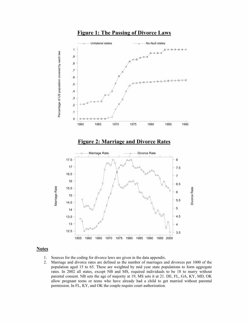
Figure 1: The Passing of Divorce Laws

Perc

enta

ge o

f US

popu

latio

n co

vere

d by

eac

h la

w

Unilateral states No-fault states

1960 1965 1970 1975 1980 1985 1990

0

.1

.2

.3

.4

.5

.6

.7

.8

.9

1

Figure 2: Marriage and Divorce Rates

Mar

riage

Rat

e

Div

orce

Rat

e

Marriage Rate Divorce Rate

1955 1960 1965 1970 1975 1980 1985 1990 1995 2000

12.5

13

13.5

14

14.5

15

15.5

16

16.5

17

17.5

3.5

4

4.5

5

5.5

6

6.5

7

7.5

8

Notes

1. Sources for the coding for divorce laws are given in the data appendix. 2. Marriage and divorce rates are defined as the number of marriages and divorces per 1000 of the

population aged 15 to 65. These are weighted by mid year state populations to form aggregate rates. In 2002 all states, except NB and MS, required individuals to be 18 to marry without parental consent. NB sets the age of majority at 19, MS sets it at 21. DE, FL, GA, KY, MD, OK allow pregnant teens or teens who have already had a child to get married without parental permission. In FL, KY, and OK the couple require court authorization.

Figure 3a: Marriage Rates by Adoption of Unilateral Divorce

Marriage rate (adopters) Marriage rate (non adopters)

1955 1960 1965 1970 1975 1980 1985 1990 1995 2000

12

13

14

15

16

17

18

19

Figure 3b: Divorce Rates by Adoption of Unilateral Divorce

Divorce rate (adopters) Divorce rate (non adopters)

1955 1960 1965 1970 1975 1980 1985 1990 1995 2000

2.5

3.5

4.5

5.5

6.5

7.5

8.5

9.5

Notes

3. See also Table 1 for when each state adopted unilateral divorce laws. In total 31 states adopted unilateral divorce between 1968 and 1985. Each series in figures 3a and 3b is calculated as a population weighted average of state level marriage and divorce rates.

Figure 4: Marriage and Divorce Rates For Adopters by Years Since Adoption of Unilateral Divorce Law

Years since implementation of unilateral divorce

Marriage Rate Divorce RateAlabama

1.61458

26.422

Alaska Arizona California Colorado Connecticut

Florida

1.61458

26.422

Georgia Hawaii Indiana Iowa Kansas

Kentucky

1.61458

26.422

Maine Massachusetts Michigan Minnesota Montana

Nebraska

1.61458

26.422

New Hampshire New Mexico North Dakota Oklahoma Oregon

-10 -5 0 5 10 15 20Rhode Island

-10 -5 0 5 10 15 201.61458

26.422

South Dakota

-10 -5 0 5 10 15 20

Texas

-10 -5 0 5 10 15 20

Washington

-10 -5 0 5 10 15 20

Wyoming

-10 -5 0 5 10 15 20

Years Since Adoption of Unilateral Divorce

Notes: The x-axis runs from 10 years prior to adoption of unilateral divorce, until 20 years after its adoption for each state. The vertical line in each chart signifies the year in which unilateral divorce was adopted. To allow the y-axis to bcomparable across states, the series for Nevada and Idaho are not shown.

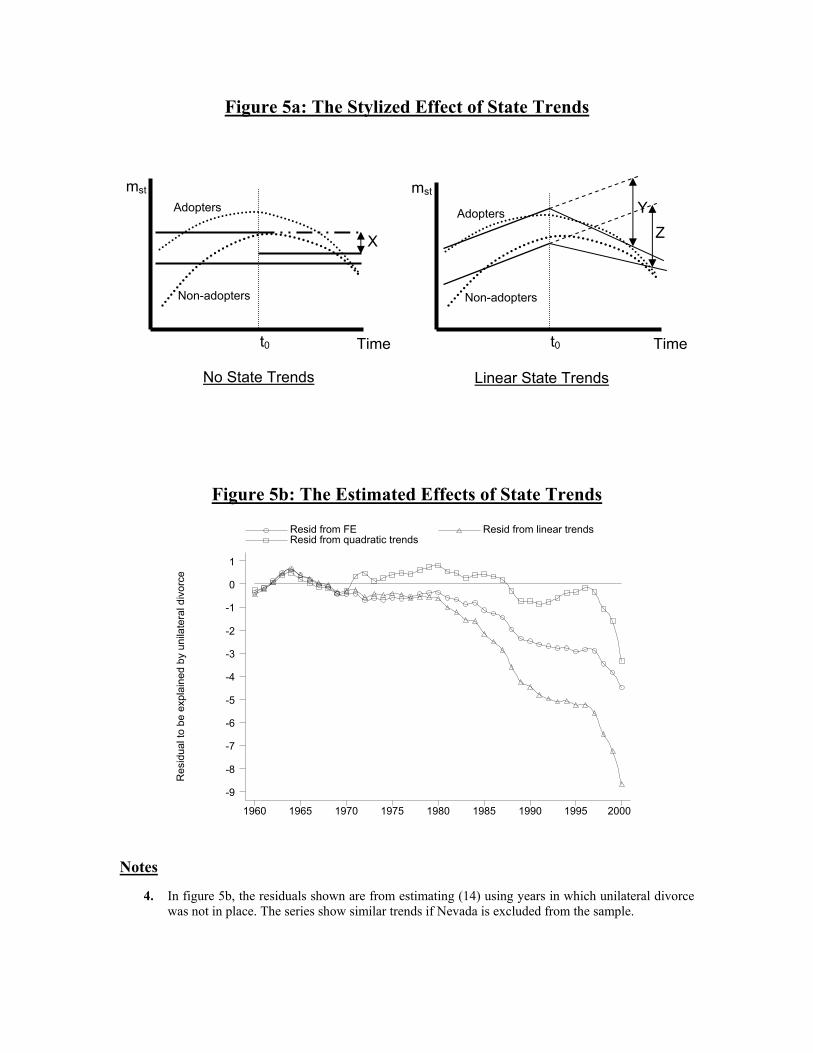
Figure 5a: The Stylized Effect of State Trends

Figure 5b: The Estimated Effects of State Trends

Res

idua

l to

be e

xpla

ined

by

unila

tera

l div

orce

Resid from FE Resid from linear trends Resid from quadratic trends

1960 1965 1970 1975 1980 1985 1990 1995 2000

-9

-8

-7

-6

-5

-4

-3

-2

-1

0

1

Notes

4. In figure 5b, the residuals shown are from estimating (14) using years in which unilateral divorce was not in place. The series show similar trends if Nevada is excluded from the sample.

Timet0

mst

Non-adopters

Adopters

X

Timet0

Non-adopters

Adopters Y Z

No State Trends Linear State Trends

mst

Notes: Years in parentheses correspond to the year of adoption of unilateral divorce law. Coding for year of adoption taken from Friedberg (1998).

CA (70)

AZ (73)

NV (73)

OR (73)

WA (73)MT (75)

ID(71)

UT

NM (73)

CO (71)

WY (77)

TX (74)

HI (73)

OK (68)

KS (69)

NE (73)

SD (85)

ND (71) MN(74)

IA (70)

MO

AR

LA

FL(71)

GA(73)

ME (73)

KY (72)TN

AL(71)MS

NC

OH

MI (72)WI

IL

NY

VA

PAIN

(73)

SC

VT

RI (76)MA (75)NH (71)

CT (73)NJ

DEMD

WV

AK (68)

Figure 6: The Adoption of Unilateral Divorce Laws Across the United States

Figure 7: Marriage and Divorce Rates by Gender and Age Cohorts

Marriage Rates for Male Age Cohorts Marriage Rates for Female Age Cohorts

Divorce Rates for Male Age Cohorts Divorce Rates for Female Age Cohorts

Aged 35-39

Aged 25-29

Mar

riage

Rat

e

Aged 15-24 Aged 25-34 Aged 35-44

1970 1975 1980 1985 1990 1995

10

20

30

40

50

60

70

Mar

riage

Rat

e

Aged 15-24 Aged 25-34 Aged 35-44

1970 1975 1980 1985 1990 1995

10

20

30

40

50

60

70

80

Div

orce

Rat

e

Aged 15-24 Aged 25-34 Aged 35-44

1970 1975 1980 1985 1990 1995

5

10

15

20

25

Div

orce

Rat

e

Aged 15-24 Aged 25-34 Aged 35-44

1970 1975 1980 1985 1990 1995

5

10

15

20

25

Notes: Cohort specific marriage and divorce rates are derived from marriage and divorce certificates data. These are only available over the period 1970 to 1995. The marriage rate for cohort c in state s in year t is defined as (divorce rates within cohorts are similarly defined);

mcst = number of individuals in cohort c that marry in state s in year t

number of individuals in cohort c in state s in year t

Figure 8: The Dynamic Effects of Unilateral Divorce on Marriage Rates

Mar

gina

l Effe

ct o

n M

arria

ge R

ate

Years Since Introduction of Unilateral Divorce

Marginal Effect Upper bound on 95% CI Lower bound on 95% CI

-4 0 5 10

-11

-9

-7

-5

-3

-1

1

3

Figure 9: Change in the Stock of Ever Married Individuals

C

hang

e in

pro

porti

on o

f pop

ulat

ion

ever

mar

ried

1955 1960 1965 1970 1975 1980 1985 1990 1995 2000

.9

1

1.1

1.2

1.3

1.4

1.5

Notes

5. Figure 8 uses the marriage rate for 15-24 year old men. The corresponding figure for women in the same age cohort is very similar.

6. The variable measured in figure 9 is the change in the ever married population, as a percentage of total annual population. This is calculated annually as two times the number of marriages minus divorces, divided by population. The aggregate figure for the US is then derived by weighting the series from each state by state population.

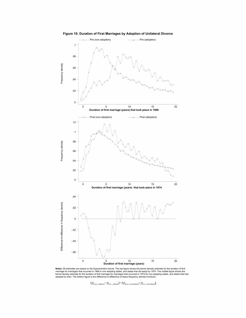
Figure 10: Duration of First Marriages by Adoption of Unilateral Divorce

Freq

uenc

y de

nsity

Duration of marriage (years)

Post (non adopters) Post (adopters)

0 5 10 15 20

0

.02

.04

.06

.08

.1

.12

Freq

uenc

y de

nsity

Duration of marriage (years)

Pre (non adopters) Pre (adopters)

0 5 10 15 20

0

.02

.04

.06

.08

.1

Diff

eren

ce-in

-diff

eren

ce in

freq

uenc

y de

nsity

Duration of marriage (years)0 5 10 15 20

-.06

-.04

-.02

0

.02

.04

Duration of first marriage (years) that took place in 1968

Duration of first marriage (years)

Duration of first marriage (years) that took place in 1974

Notes: All estimates are based on the Epanechnikov kernel. The top figure shows the kernel density estimate for the duration of first marriage for marriages that occurred in 1968 in non-adopting states, and states that did adopt by 1974. The middle figure shows the kernel density estimate for the duration of first marriage for marriages that occurred in 1974 for non-adopting states, and states that had adopted by then. The bottom figure is the difference-in-difference of these frequency density functions;

)()( ____ nonadopterprenonadopterpostadopterpreadopterpost pppp −−−

Table 1: Family Law Across the United States

State

1960s 1970s 1980s 1990s 1960s 1970s 1980s 1990s

Alabama 1971 1971 18.6 20.9 17.8 15.7 6.4 9.3 9.7 9.3 1.73 AlabamaAlaska 1968 1935 14.7 18.1 17.6 13.7 6.6 10.9 10.7 7.7 0.17 Alaska

Arizona 1973 1937 13.7 18.5 16.5 14.5 9.2 11.6 10.6 9.5 1.09 ArizonaArkansas - 1931 17.9 19.4 21.0 23.7 6.1 10.9 10.9 10.6 0.99 ArkansasCalifornia 1970 1970 11.7 12.1 12.8 10.3 5.6 8.7 7.6 10.14 CaliforniaColorado 1971 1972 16.3 17.1 15.9 13.5 5.9 9.0 8.7 8.1 1.18 Colorado

Connecticut 1973 1973 11.9 12.1 12.4 10.7 2.2 5.1 5.7 4.7 1.37 ConnecticutDelaware - 1957 10.1 11.3 12.5 11.0 2.7 6.7 7.0 6.9 0.26 Delaware

District of Columbia - 1966 16.5 11.2 11.7 9.6 2.9 6.7 6.9 4.9 0.34 District of ColumbiaFlorida 1971 1971 14.2 17.5 17.5 16.5 7.3 11.2 10.6 9.4 3.89 Florida

Georgia 1973 1973 21.5 21.2 18.0 13.2 4.6 8.3 8.5 7.8 2.41 GeorgiaHawaii 1973 1965 14.7 17.8 21.2 24.7 3.4 7.1 6.6 6.4 0.40 Hawaii

Idaho 1971 1945 32.1 25.0 20.9 20.5 7.3 9.7 10.2 9.4 0.39 IdahoIllinois - 1984 15.3 15.8 13.0 11.8 4.0 6.5 6.4 5.5 5.15 Illinois

Indiana 1973 1973 16.7 17.2 14.8 12.0 6.0 10.3 9.8 2.44 IndianaIowa 1970 1970 13.7 15.0 14.0 13.0 3.4 5.4 5.9 5.9 1.33 Iowa

Kansas 1969 1969 14.0 16.5 15.4 12.9 4.5 7.9 8.1 7.3 1.09 KansasKentucky 1972 1962 15.5 15.7 17.2 18.2 4.2 6.3 7.5 8.7 1.61 KentuckyLouisiana - 1916 13.7 16.1 14.2 13.8 4.9 1.78 Louisiana

Maine 1973 1973 15.0 17.6 16.2 13.2 4.4 7.6 7.8 6.5 0.51 MaineMaryland - 1969 21.0 17.7 15.2 12.6 3.1 5.2 5.4 4.9 1.84 Maryland

Massachusetts 1975 1975 11.8 12.1 12.4 10.6 2.3 4.1 4.7 3.7 2.65 MassachusettsMichigan 1972 1972 15.3 15.3 13.1 11.1 4.1 6.8 6.6 6.2 4.08 Michigan

Minnesota 1974 1933 13.0 13.4 13.0 10.9 2.6 5.0 5.5 5.2 1.83 MinnesotaMississippi - 1978 17.5 19.4 15.9 13.0 4.6 7.9 8.0 8.1 1.13 Mississippi

Missouri - 1974 15.2 17.3 15.9 13.3 5.1 7.7 8.0 7.6 2.24 MissouriMontana 1975 1973 13.1 16.2 14.3 12.4 5.3 8.8 8.6 7.2 0.35 Montana

Nebraska 1972 1972 14.5 14.8 13.0 12.1 3.1 5.5 6.3 6.1 0.72 NebraskaNevada 1973 1931 295.8 262.5 171.4 133.3 37.7 26.1 21.1 12.8 0.33 Nevada

New Hampshire 1971 1971 21.9 18.2 16.0 12.5 4.0 7.5 7.4 7.2 0.39 New HampshireNew Jersey - 1971 11.0 11.6 11.8 10.6 1.5 4.1 5.4 4.8 3.28 New JerseyNew Mexico 1973 1933 19.4 21.4 16.6 13.1 5.3 11.1 11.6 9.0 0.55 New Mexico

New York - 1967 12.2 12.7 13.3 12.5 0.8 4.2 5.4 4.8 8.31 New YorkNorth Carolina - 1910 13.0 13.0 12.0 11.9 3.1 5.8 7.3 7.5 2.61 North Carolina

North Dakota 1971 1971 12.7 14.6 13.1 11.4 2.0 4.1 5.4 5.3 0.30 North DakotaOhio - 1974 12.5 14.4 13.9 12.4 4.3 7.4 7.4 6.8 4.89 Ohio

Oklahoma 1968 1953 21.6 23.9 18.9 13.8 8.3 11.6 11.6 10.3 1.30 OklahomaOregon 1973 1971 11.4 13.3 13.0 12.5 5.9 9.3 9.2 7.7 1.08 Oregon

Pennsylvania - 1980 11.1 12.4 11.5 10.0 2.3 4.2 5.0 5.1 5.53 PennsylvaniaRhode Island 1976 1910 11.5 12.0 12.3 11.8 1.9 4.4 5.6 5.2 0.44 Rhode Island

South Carolina - 1969 29.6 30.3 24.4 19.5 2.2 5.0 6.3 6.2 1.36 South CarolinaSouth Dakota 1985 1985 20.7 26.7 18.0 16.1 2.5 4.9 6.0 6.2 0.33 South Dakota

Tennessee - 1963 16.0 20.0 19.0 22.0 4.8 8.8 9.6 9.5 2.00 TennesseeTexas 1974 1910 17.6 19.8 18.3 15.2 6.5 9.0 9.3 7.7 6.08 Texas

Utah - 1943 15.8 19.8 18.2 17.1 5.0 7.7 8.6 7.5 0.60 UtahVermont - 1969 15.4 16.2 16.0 15.4 2.5 5.6 6.9 6.8 0.22 VermontVirginia - 1960 16.2 17.2 16.5 15.1 3.2 5.4 6.4 6.6 2.35 Virginia

Washington 1973 1921 18.0 18.4 15.6 12.3 6.4 10.0 9.3 8.1 1.76 WashingtonWest Virginia - 1969 13.1 15.1 12.2 10.1 3.7 6.8 7.9 7.8 0.89 West Virginia

Wisconsin - 1977 11.5 13.1 13.0 11.1 2.2 4.5 5.5 5.3 2.10 WisconsinWyoming 1977 1977 18.5 23.3 17.8 15.6 7.5 10.6 11.4 9.9 0.18 Wyoming

United States 15.2 16.4 15.4 13.8 4.1 7.1 7.5 6.9 United States

Year of Enactment of Family Law

Percentage of US Population

Marriage Rate Divorce RateUnilateral Divorce No Fault Divorce

Notes: Legal definitions are given in the data appendix. Arizona and Louisiana reverted back to fault based covenant marriages in 1997. Marriage rate data is available for 1957-2000, except Mississippi which starts in 1958. Incomplete divorce rate data is for CA 91-00, CO 95-00, IL 56-57, IN 91-00, KT 56-58, LO 56-70, 84-00, MA 56, NY 56-57, NC 56-57 and WV 56-57. The marriage (divorce) rate is defined as the number of marriages (divorces) per 1000 of the adult population (aged 15 to 65). Decennial averages are calculated if there at least five state observations. The decennial US average is calculated by weighting state averages by mid year population estimates. The column showing the state percentage of US population is an average calculated over the period 1960-2000.

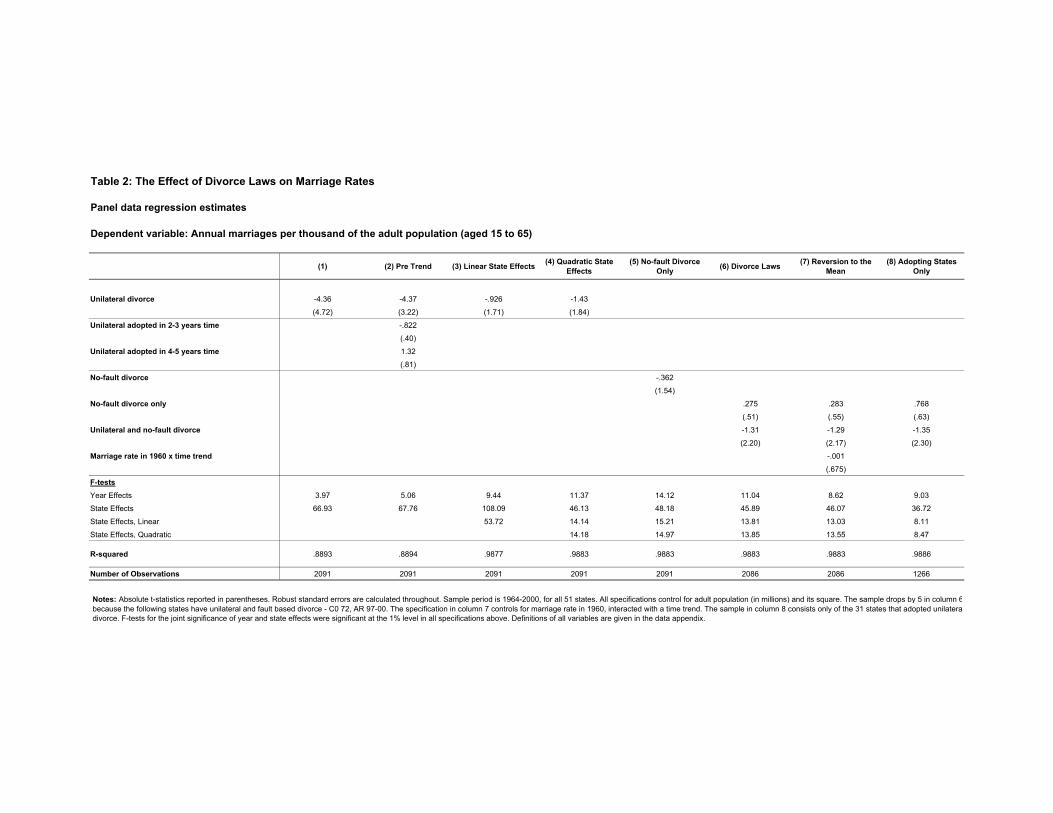
Table 2: The Effect of Divorce Laws on Marriage Rates

Panel data regression estimates

Dependent variable: Annual marriages per thousand of the adult population (aged 15 to 65)

(1) (2) Pre Trend (3) Linear State Effects (4) Quadratic State Effects

(5) No-fault Divorce Only (6) Divorce Laws (7) Reversion to the

Mean(8) Adopting States

Only

Unilateral divorce -4.36 -4.37 -.926 -1.43

(4.72) (3.22) (1.71) (1.84)

Unilateral adopted in 2-3 years time -.822

(.40)

Unilateral adopted in 4-5 years time 1.32

(.81)

No-fault divorce -.362

(1.54)

No-fault divorce only .275 .283 .768

(.51) (.55) (.63)

Unilateral and no-fault divorce -1.31 -1.29 -1.35

(2.20) (2.17) (2.30)

Marriage rate in 1960 x time trend -.001

(.675)

F-testsYear Effects 3.97 5.06 9.44 11.37 14.12 11.04 8.62 9.03

State Effects 66.93 67.76 108.09 46.13 48.18 45.89 46.07 36.72

State Effects, Linear 53.72 14.14 15.21 13.81 13.03 8.11

State Effects, Quadratic 14.18 14.97 13.85 13.55 8.47

Number of Observations 2091 2091 2091 2091 2091 2086 2086 1266

R-squared .8893 .8894 .9886.9883 .9883.9877 .9883 .9883

Notes: Absolute t-statistics reported in parentheses. Robust standard errors are calculated throughout. Sample period is 1964-2000, for all 51 states. All specifications control for adult population (in millions) and its square. The sample drops by 5 in column 6because the following states have unilateral and fault based divorce - C0 72, AR 97-00. The specification in column 7 controls for marriage rate in 1960, interacted with a time trend. The sample in column 8 consists only of the 31 states that adopted unilateradivorce. F-tests for the joint significance of year and state effects were significant at the 1% level in all specifications above. Definitions of all variables are given in the data appendix.

Table 3: Robustness Checks

Panel data regression estimates

Dependent variable: Annual marriages per thousand of the adult population (aged 15 to 65)

(1) Abortion (2) Joint Custody

(3) Non Common Law Marriage

States

(4) Adopting States Only

(5) Regional Fixed Effects

(6) Early Adopters Only

(7) Neighboring Adopting States

(8) Low Out-of-wedlock Births

(9) High Out-of-wedlock Births

No-fault divorce only .360 .407 .766 1.77 .283 .004 .486 -.291 .534

(.66) (.74) (1.07) (1.06) (.55) (.02) (.92) (1.40) (.71)

Unilateral and no-fault divorce -1.29 -1.28 -1.75 -1.55 -1.29 -.844 -1.29 -.662 -3.16

(2.17) (2.15) (2.34) (1.87) (2.17) (3.02) (2.03) (2.07) (1.76)

Legalized abortion -1.10 -1.11 -1.90 -3.42

(1.85) (1.87) (2.46) (2.69)

Joint Custody -.484 -.475 -.931

(1.45) (1.11) (1.41)

-.001

(1.02)

.001

(1.26)

Regional FE Yes Yes Yes

Number of Observations 2086 2086 1595 939 2086 1393 2004 1065 1021

Endogenous Divorce Law

.9167 .9888

Neighboring states that adopt (weighted by the area of the adopting neighboring states in 1000 sq km)

Neighboring states that adopt x area of state s (in 1000 sq km)

.9883 .9372R-squared .9884

Endogenous Timing of Adoption

.9884 .9884 .9887 .9889

Omitted Policies

Notes: Absolute t-statistics reported in parentheses. Robust standard errors are calculated throughout. All specifications control for adult population (in millions) and its square. Column 3 restricts the sample to only include states that do not allow common law marriage. Column 4 further restricts the sample to only include adopting states. In columns 5 to 7, regional fixed effects are also controlled for. The regions are defined using a standard classification of Pacific, Mountain, West North Central, East North Central, Middle Atlantic, New England, West South Central, East South Central, and South Atlantic. In column 6, early adopters are defined as those states that adopted unilateral divorce up to and including 1972. Alaska and Hawaii are dropped form the neighboring states specification in column 7. In columns 8 and 9 I split the sample by the percentage of total births that occur out-of-wedlock in 1970. Low out-of-wedlock states have less than the median percentage of births out-of-wedlock. F-tests for the joint significance of year and state effects were significant at the 1% level in all the specifications above. Definitions of all variables are given in the data appendix.

Table 4: The Effect of Divorce Laws on Marriage Rates Within Cohorts

Panel data regression estimates

Dependent variable: Annual marriages per thousand of the cohort population

Men

(1) 15-24 Year Olds

(2) 25-34 Year Olds

(3) 35-44 Year Olds

(4) First Marriage (15-34 year olds)

(5) Second Marriage (25-44 year olds)

(6) White (15-44 year olds)

(7) Black (15-44 year olds)

No-fault divorce only .129 .578 .118 -.552 .400 .895 -3.23(.21) (1.34) (.33) (1.19) (1.80) (1.07) (1.52)

Unilateral and no-fault divorce -1.37 -.170 -.988 -1.22 -.243 -3.06 -1.46(1.90) (.33) (1.86) (2.52) (.71) (3.50) (.49)

Number of Observations 1109 1109 1109 1087 998 896 783

Women

(1) 15-24 Year Olds

(2) 25-34 Year Olds

(3) 35-44 Year Olds

(4) First Marriage (15-34 year olds)

(5) Second Marriage (25-44 year olds)

(6) White (15-44 year olds)

(7) Black (15-44 year olds)

No-fault divorce only .726 .181 .136 -.178 .048 1.32 -2.64(.97) (.45) (.47) (.38) (.23) (1.41) (1.20)

Unilateral and no-fault divorce -1.66 .032 -.809 -1.32 -.293 -3.38 2.84(1.90) (.06) (1.84) (2.65) (.91) (3.53) (.72)

Number of Observations 1109 1109 1109 1087 998 896 730

Age Marriage Number

R-squared .9823 .9587 .9488

Race

.9486 .9014.9614 .9625

.9509 .9393R-squared .9788 .9724 .9588 .9605 .9622

Notes: Absolute t-statistics reported in parentheses. Robust standard errors are calculated throughout. Cohort specific marriage and divorce rates are derived from marriage and divorce certificates data. These are only available over the period 1970 to 1995. All specifications control for the female to male sex ratio in the appropriate age group, and include quadratic state trends over time. Definitions of all variables are given in the data appendix.