The Impact of Crop Minimum Support Prices on Crop ... · Chintapalli and Tang: Impact of minimum support prices in the presence of strategic farmers 3 In this paper we develop a parsimonious

Electronic copy available at: https://ssrn.com/abstract=3024583

The Impact of Crop Minimum Support Prices onCrop Selection and Farmer Welfare in the presence of

Strategic Farmers

Prashant Chintapalli Christopher S. TangUCLA Anderson School of Management

In many developing countries, governments often use Minimum support prices (MSPs) as interventions to

(i) safeguard farmers’ income against crop price falls, and (ii) ensure sufficient and balanced production of

different crops. In this paper, we examine two questions: (1) What is the impact of MSPs on the farmers’

crop selection and production decisions, future crop availabilities, and farmers’ expected profits? (2) What

is the impact of strategic farmers on crop selection and production decisions, future crop availabilities, and

farmers’ expected profits? To explore these questions, we present a model in which the market consists of

two types of farmers (with heterogeneous production costs): myopic farmers (who make their crop selection

and production decisions based on recent market prices) and strategic farmers (who make their decisions by

taking all other farmers’ decisions into consideration). By examining the dynamic interactions among these

farmers for the case when there are two (complementary or substitutable) crops for each farmer to select to

grow, we obtain the following results. First, we show that, regardless of the values of the MSPs offered to the

crops, the price disparity between the crops worsens as the complementarity between the crops increases.

Second, we find that MSP is not always beneficial. In fact, offering MSP for a crop can hurt the profit of

those farmers who grow that crop especially when the proportion of strategic farmers is sufficiently small.

Third, a bad choice of MSPs can cause the expected quantity disparity between crops to worsen. By taking

these two drawbacks of MSPs into consideration, we discuss ways to select effective MSPs that can improve

farmers’ expected profit and reduce quantity disparity between crops.

Key words : Minimum support prices, subsidies, agricultural supply chains, government and public policy

History :

1. Introduction

In many developing countries, the agricultural sector is important because: (1) it offers

a source of income to a large number of small rural households, and (2) it provides a

stable food supply for the country. As such, developing efficient and effective agro-policies

to improve farmers’ earnings and to stabilize crop availabilities and prices are critical

(Thorbecke 1982). While governments in developing countries design and develop a wide

variety of agro-policies ranging from input subsidies (for seeds and fertilizers, power, etc.)

to output subsidies (for storage and transportation), in this paper, we shall focus on a

particular type of output subsidies that is called the Minimum Support Price (MSPs).

MSPs for different crops are offered by governments in many developing countries like

Bangladesh, Brazil, China, India, Pakistan, and Thailand. For example, in 2017, the Indian

1

Electronic copy available at: https://ssrn.com/abstract=3024583

Chintapalli and Tang: Impact of minimum support prices in the presence of strategic farmers2

government offers MSPs for 23 crops, which comprise 7 cereals, 5 pulses (grain seeds of

legumes), 7 oil seeds, and 4 commercial crops. Essentially, MSP of a crop serves as a form

of “contingent subsidy” to farmers who grow that crop: when the market price of a crop

falls below its MSP, government purchases the crop from the farmers at the pre-announced

MSP of the crop by absorbing the price shortfall (i.e., the difference between the market

price and the MSP). By guaranteeing minimum prices for certain crops, a government

intends to provide incentives for farmers to grow a more balanced mixture of crops.

This paper examines the implications of MSPs on: (1) farmers’ earnings, and (2) quantity

disparity between two crops. Our model is based on the setting of a developing country.

To motivate our research questions involving MSPs, let us consider the role played by

MSPs in the Indian agricultural sector. MSPs have been introduced as a part of the Green

Revolution in 1965 when India’s cereal imports reached an alarming stage. This event has

triggered the Indian government to establish the Commission for Agricultural Costs &

Prices (CACP) with the mandate to develop crop-price policies. As a part of these reforms,

MSPs were introduced as incentives to benefit Indian farmers and consumers by increasing

food supply at affordable prices (Chand 2003, Malamasuri et al. 2013).1 With an efficient

MSP scheme developed by CACP over the years, India evolved from a grain “deficient”

country in mid-1960’s to a grain “surplus” country by early 1980’s. However, due to the

fact that MSPs in India were geared towards rice and wheat production, there was a severe

shortage of coarse cereals and oil seeds (Chand 2003, Parikh and Chandrashekhar 2007) and

an over-production of rice and wheat. Such an imbalance in the availability of agricultural

commodities can lead to micro-nutrient malnutrition (or hidden hunger) (Byerlee et al.

2007). This observation suggests that the efficacy of MSPs should be measured in terms

of the availability of different crops and the farmers’ expected earnings.

1 When determining MSPs, CACP takes into account six factors, namely (i) demand and supply, (ii) cost of production,(iii) market price trends, (iv) inter-crop price parity, (v) terms of trade between agriculture and non-agriculture, and(vi) likely implications of MSP on consumers of that product (Commission for Agricultural Costs & Prices 2017). Inour analysis we take into account the factors (i), (ii), (iii), (iv) and (vi). We account for the supply through consideringthe response of the farmers’ sowing decisions towards the MSPs announced. We account for the demand through theinverse demand functions of the crops. By assuming that the farmers are heterogeneous in their production costs forthe two crops, we account for (ii). Based on his type – strategic or myopic – each farmer considers the past price ofthe crops in a specific way. Thus, we account for (iii) through farmers’ perceptions of past prices. We account for (iv)through farmers’ individual rationality and their choice of the crops in the light of the past prices and the MSPs ofthe crops. Finally, we account for (vi) by analyzing the impact of MSP, in confluence with the past market prices,on the future market prices. Thus, we make an attempt to develop a unified framework using a parsimonious modelwith two crops to comprehensively capture the main features of an MSP scheme.


In this paper we develop a parsimonious model to analyze the impact of MSPs on farmers’

earnings, crop availabilities, and crop prices by considering a setting in which there are

two (complementary or substitutable) crops from which each farmer can choose one crop

to cultivate. In addition to heterogeneous production costs for each crop, we also consider

the case when the market is comprised of myopic farmers (who make their crop selection

and production decisions based on recent market pries) and strategic farmers (who make

their decisions by taking all other farmers’ decisions into consideration). By examining

the dynamic interactions among myopic and strategic farmers, our model enables us to

examine two research questions:

1. What is the impact of MSPs on the farmers’ crop selection and production decisions,

future crop availabilities, and farmers’ expected revenues?

2. What is the impact of strategic farmers on crop selection and production decisions,

future crop availabilities, and farmers’ expected revenues?

Our equilibrium analysis enables us to obtain the following results. First, we find in

Corollaries 1 and 6 that, regardless of the values of MSPs, the price disparity between the

crops worsens as the complementarity between the crops increases. Second, we show in

Proposition 5 that MSP is not always beneficial. In Proposition 5, specifically, we show that

moderately low MSP for a crop will degrade the expected profits of the farmers growing

the crop if the number of strategic farmers is very small. Thus, choosing an inappropriate

MSP for a crop, especially when there are very few strategic farmers, can actually defeat

the intended goal of offering MSP for the crop, which is to benefit the farmers growing

the crop. Also, we show in Proposition 4 that when the proportion of strategic farmers is

small, offering moderately low MSP for a crop can actually cause fewer strategic farmers

to grow that crop. Third, in Proposition 3, we find that the total production of a crop is

increasing in the MSP offered for the crop. Therefore, a bad choice of MSPs can cause the

production quantity disparity between crops to worsen. Hence, to reduce quantity disparity

between crops, a carefully designed MSP policy is critical. Finally, through formulating

an optimization problem for a policy-maker to choose crop MSPs in order to maximize

social welfare, we illustrate that offering MSPs to complementary (i.e., dissimilar) crops

has the potential to achieve higher social welfare at a lower expected expenditure to the

policy-maker.


The paper is organized as follows. Section 2 reviews literature related to MSPs. In Section

3 we introduce the model and discuss various assumptions. To explicate our analysis about

myopic and strategic farmers’ crop selection and production decisions, we examine the case

when MSPs are not present in Section 4. Section 5 extends our analysis to the case when

MSPs are present. In Section 6 we formulate and discuss the optimization problem of the

government whose objective is to set MSPs in order to improve farmers’ welfare and crop

balance. We conclude in Section 7.

2. Literature Review

Our research pertains to agro-policies that affect both crop selection and crop production

by myopic and strategic farmers. The literature on MSPs is vast in the agricultural eco-

nomics discipline and the reader is referred to Tripathi et al. (2013) and the references

therein for a good synopsis on MSPs in developing countries. Without accounting for the

price interactions between crops with MSP support and those crops without MSP support,

Fox (1956) develops macro-economics analysis to evaluate the impact of MSPs and finds

that MSPs can mitigate the fall in GNP during a recession. Dantwala (1967) finds that

in spite of the increasing MSPs, the crop market prices continue to rise. More recently,

Subbarao et al. (2011) shows evidence that the increase in market price is caused by the

increase in MSPs. In the same vein, Chand (2003) presents qualitative assessment of the

ill-effects of the wheat- and-rice-centric MSPs on the Indian economy. Chhatre et al. (2016)

point out that many farmers in India moved to cultivating high-yield varieties of rice and

wheat due to the wheat- and-rice-centric MSPs offered by the Indian government. The

authors also identify the various socio-economic and environmental problems associated

with an improper choice of MSPs. Besides the Indian context, Spitze (1978) analyzes the

impact of federal policy (The Food and Agriculture Act of 1977) on agriculture in the

United States. The author states that continuous improvement in gathering and analyzing

information is a prerequisite for the design of effective MSPs.

Recent papers on agricultural operations in OM literature include: (i) Tang et al. (2015),

Chen and Tang (2015), Parker et al. (2016), Liao et al. (2017) focus on the economic value

of disseminating agricultural information to the farmers, (ii) Kazaz and Webster (2011),

Dawande et al. (2013), Huh and Lall (2013) examine the issue of resource and inventory

management, (iii) Huh et al. (2012), Federgruen et al. (2015), An et al. (2015) focus on


contract farming and farmer aggregation, and (iv) Hu et al. (2016), Alizamir et al. (2015),

Guda et al. (2016) examine social responsibility and public policy issues arising from the

agricultural sector.

While our paper is related to group (iv), it differs from the these papers in the following

manner. First, Hu et al. (2016) focus on the value of strategic farmers in the context of

a single crop with a deterministic demand function. They show that a tiny fraction of

strategic farmers can stabilize the steady state prices. They also extend their analysis to

two crops with independent market prices. In contrast, our goal is to evaluate the impact

of MSPs on farmers’ crop selection and production decisions, and on the market prices of

two crops with dependent and yet stochastic market price.

Second, Alizamir et al. (2015) focus on the impact of federal policy on agriculture indus-

try in the United States. They compare two schemes (Price Loss Coverage (PLC) and the

Agriculture Risk Coverage (ARC) programs) with respect to (i) farmers’ welfare, (ii) fed-

eral expenditure, and (iii) consumer welfare. While PLC is akin to MSP, our paper differs

from Alizamir et al. (2015) in three aspects. First, they assume there are finite number

of farmers, and the production of each farmer can affect the market price (i.e., farmers

are price setters). In contrast, our context is that of developing countries, and we consider

infinitesimally small farmers whose individual decisions do not affect the market price (i.e.,

farmers are price-takers). Second, they analyze the case of only one crop, while we consider

two crops that can be substitutes or complements. Hence, by capturing the interaction

between two crops in our model, we analyze the simultaneous impact of the MSP of each

crop on the production of both the crops. Third, they do not consider the existence of

myopic and strategic farmers, while we consider a mixture of both myopic and strategic

farmers in our model. Our model fits well in the context of developing countries where

a large portion of the farming communities are smallholders who are myopic: their crop

selection and production decisions are purely based on the most recently oberved market

price.

Finally, Guda et al. (2016) examine the role of MSPs in emerging economies, but there

are two fundamental differences between our paper and theirs. The first difference is that

we assume heterogeneity in farmers’ production costs, while they assume homogeneous pro-

duction costs. In general, the cost of cultivating a crop can vary across farmers depending

on the local soil, the climatic conditions, and the farming practices they employ. Second,


they consider a single crop and relegate the case of multiple crops as future research due to

the inherent complexity. As such, our paper attempts to examine the impact of the MSPs

of two crops on the availabilities of one another.

3. Model Preliminaries

We consider two crops (A and B) to be produced by heterogeneous farmers whose pro-

duction costs are uniformly distributed over the interval [−0.5,0.5] as in the Hotelling’s

model. These two crops can be substitutes (e.g., rice and wheat) or complements (e.g., rice

and pulses/lentils). For a farmer located at x ∈ [−0.5,0.5], his costs of producing crops A

and B are given by cA(x) = x+ 0.5 and cB(x) = 0.5− x, respectively. We assume that the

farmers are infinitesimally small so that each farmer can produce 1 unit of a crop and each

farmer is a price taker.

In our model, the market price of a crop depends on the available quantity of the crop.

Let qkTt denote the “total” availability of crop k ∈ {A,B} in period t and let pkt denote the

market price of crop k ∈ {A,B} in period t. For ease of exposition, we normalize the size

of markets to 1 so that qkTt 6 1 for k ∈ {A,B}. Throughout this paper, we assume that the

market price ptk for crop k ∈ {A,B} in period t satisfies:

pAt = a− ρqATt −αqBTt + εAt =E[pAt ] + εAt , and

pBt = a−αqATt − ρqBTt + εBt =E[pBt ] + εBt , (1)

where ρ (> 0) is the price sensitivity, and α is a measure of substitutability (if α > 0) or

complementarity (if α < 0) between the two crops. As commonly assumed in the litera-

ture for substitutable/complementary products, we shall assume that α< ρ. The random

variables εkt (k ∈ {A,B}) denote the market uncertainty in period t. We assume εkt are

iid (across t and k) with mean 0, variance σ2 and with distribution and density functions

F (·) and f(·), respectively.2 We also assume that the distribution F (·) has support over a

range of value so that the market price pkt in non-negative. Let F (·) = (1−F (·)) denote the

complementary cumulative distribution of εkt . The expected profit of a farmer at location

x who grows crop k ∈ {A,B} is given by:

Πkt (x) = E[pkt ]− ck(x) = a− ρqkTt −αq

jTt − ck(x), j 6= k. (2)

2 To keep the notation simple, we assume that εAt and εBt follow the same distribution. However, our analysis can beextended to the case of different distributions.


For ease of exposition, we define r≡ ρ−α (> 0), so that r measures the “dissimilarity”

between the two crops, and φ≡ a− ρ+α2

, which corresponds to the expected market price

when half of the market grows A (grows B) (i.e., when qATt = qBTt = 0.5). Finally, wherever

applicable, we denote the price vector in period t by Pt = [pAt , pBt ]T . To simplify our expo-

sition and our analysis (e.g., by ruling out the boundary equilibrium solution), we shall

make the following assumptions:

Assumption 1. In each period, each farmer will not be idle and will select exactly one

crop to grow.

First, the non-idling assumption is reasonable especially when the farmer’s production

cost is lower than the market price pkt in general. Second, due to economies of scale, small

land-holders in emerging markets cannot afford to grow multiple crops.

Next, let ∆pt be the price disparity between crops A and B in period t. By applying (1)

and the fact that r= ρ−α, we obtain:

∆pt = pAt − pBt =−r(qATt − qBTt ) + ξt, ∀t,

where ξt = εAt − εBt . To ensure that the price disparity ∆pt is stable over time so that we

can rule out boundary equilibrium solution, we shall make the following assumption.

Assumption 2. The dissimilarity between two crops r satisfies: 0 < r ≡ (ρ − α) < 1.

Also, the variance of the market uncertainty is sufficiently less than 1 (i.e., σ2 << 1).

Since, r measures the “dissimilarity” between two crops, we can treat the crops to be

substitutes if r is small and to be complements if r is large. Furthermore, because 0< r < 1

, |qAt −qBt |6 1, and E[ξt] = 0, it is easy to check that |E[∆pt]|6 r < 1, for all t. Furthermore,

when |E[∆pt]|6 1 and σ2 << 1, we can ascertain that |∆pt|< 1 nearly always holds so that

we can effectively assume P(|∆pt|< 1)u 1.3

3 We formalize this finding in the lemma below.

Lemma 1. Let the random variable X ∼U [−β,β] denote the type of the farmer so that the production costs of cropsA and B for farmer who is located at X = x are given by x+β and β−x respectively. Then,

P(|pAt − pBt |> 2β

)6 P (|ξt|> 2β(1− r))6 σ2

2β2(1− r)2, where ξt = εAt − εBt .

Hence, for a given r ∈ (0,1), we have P (|∆pt|> 2β)→ 0 if β >> σ.

Without loss of generality, we scale β to 1 in our model and assume that σ is sufficiently small (i.e., σ << 1). Hence,by virtue of Lemma 1, there will be a positive production of each crop in every period.


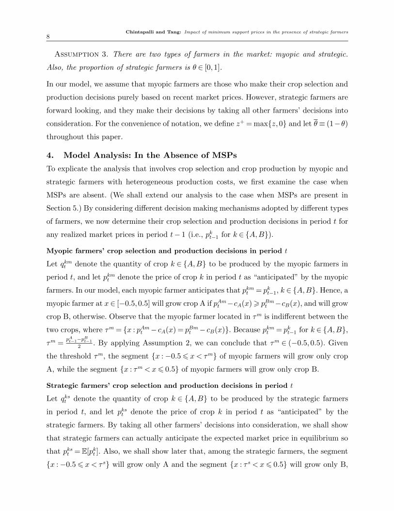
Assumption 3. There are two types of farmers in the market: myopic and strategic.

Also, the proportion of strategic farmers is θ ∈ [0,1].

In our model, we assume that myopic farmers are those who make their crop selection and

production decisions purely based on recent market prices. However, strategic farmers are

forward looking, and they make their decisions by taking all other farmers’ decisions into

consideration. For the convenience of notation, we define z+ = max{z,0} and let θ≡ (1−θ)throughout this paper.

4. Model Analysis: In the Absence of MSPs

To explicate the analysis that involves crop selection and crop production by myopic and

strategic farmers with heterogeneous production costs, we first examine the case when

MSPs are absent. (We shall extend our analysis to the case when MSPs are present in

Section 5.) By considering different decision making mechanisms adopted by different types

of farmers, we now determine their crop selection and production decisions in period t for

any realized market prices in period t− 1 (i.e., pkt−1 for k ∈ {A,B}).

Myopic farmers’ crop selection and production decisions in period t

Let qkmt denote the quantity of crop k ∈ {A,B} to be produced by the myopic farmers in

period t, and let pkmt denote the price of crop k in period t as “anticipated” by the myopic

farmers. In our model, each myopic farmer anticipates that pkmt = pkt−1, k ∈ {A,B}. Hence, a

myopic farmer at x∈ [−0.5,0.5] will grow crop A if pAmt −cA(x)> pBmt −cB(x), and will grow

crop B, otherwise. Observe that the myopic farmer located in τm is indifferent between the

two crops, where τm = {x : pAmt − cA(x) = pBmt − cB(x)}. Because pkmt = pkt−1 for k ∈ {A,B},τm =

pAt−1−pBt−1

2. By applying Assumption 2, we can conclude that τm ∈ (−0.5,0.5). Given

the threshold τm, the segment {x :−0.56 x < τm} of myopic farmers will grow only crop

A, while the segment {x : τm <x6 0.5} of myopic farmers will grow only crop B.

Strategic farmers’ crop selection and production decisions in period t

Let qkst denote the quantity of crop k ∈ {A,B} to be produced by the strategic farmers

in period t, and let pkst denote the price of crop k in period t as “anticipated” by the

strategic farmers. By taking all other farmers’ decisions into consideration, we shall show

that strategic farmers can actually anticipate the expected market price in equilibrium so

that pkst = E[pkt ]. Also, we shall show later that, among the strategic farmers, the segment

{x :−0.56 x < τ s} will grow only A and the segment {x : τ s < x6 0.5} will grow only B,


where τ s ≡ τ s(pAst , pBst ) = {x : pAst −cA(x) = pBst −cB(x)}. (We shall determine the threshold

τ s value in Proposition 1).

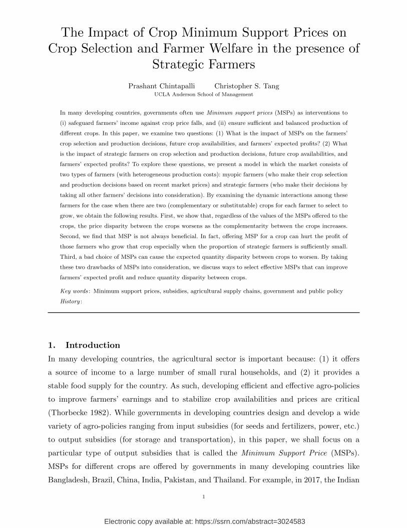
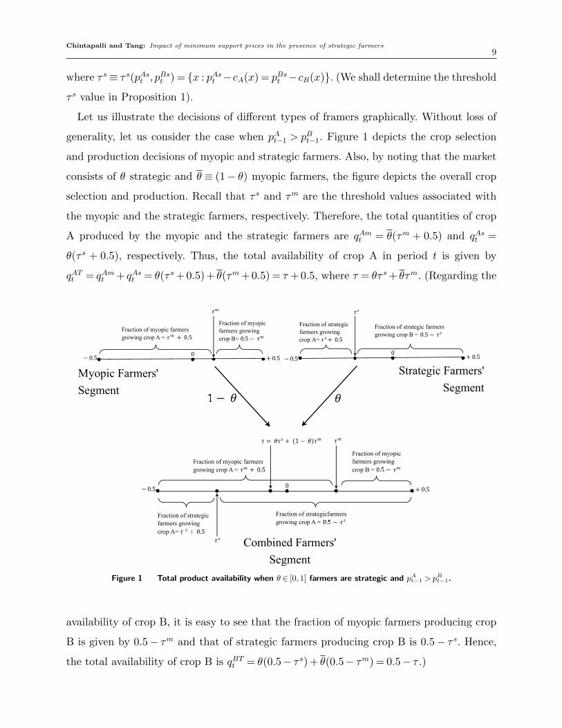
Let us illustrate the decisions of different types of framers graphically. Without loss of

generality, let us consider the case when pAt−1 > pBt−1. Figure 1 depicts the crop selection

and production decisions of myopic and strategic farmers. Also, by noting that the market

consists of θ strategic and θ ≡ (1− θ) myopic farmers, the figure depicts the overall crop

selection and production. Recall that τ s and τm are the threshold values associated with

the myopic and the strategic farmers, respectively. Therefore, the total quantities of crop

A produced by the myopic and the strategic farmers are qAmt = θ(τm + 0.5) and qAst =

θ(τ s + 0.5), respectively. Thus, the total availability of crop A in period t is given by

qATt = qAmt + qAst = θ(τ s + 0.5) + θ(τm + 0.5) = τ + 0.5, where τ = θτ s + θτm. (Regarding the

�− �

Fraction of myopic

farmers growing

crop B = 0 − ��

Fraction of strategicfarmers

growing crop A = − ��

Fraction of strategic

farmers growing

crop A= � � 0.5

��

��

− 0.5 + 0.50

� = �� + (1 − �)��

Fraction of myopic farmers

growing crop A = �� + 0.5

Fraction of myopic farmers

growing crop A = �� + 0.5

Fraction of myopic

farmers growing

crop B= 0.5 − � �

��

− 0.5 + 0.50

Fraction of strategic

farmers growing

crop A= � �+ 0.5

+ 0.50

��

Fraction of strategic farmers

growing crop B = 0.5 − � �

− 0.5

Myopic Farmers'

Segment

Strategic Farmers'

Segment

Combined Farmers'

Segment

Figure 1 Total product availability when θ ∈ [0,1] farmers are strategic and pAt−1 > pBt−1.

availability of crop B, it is easy to see that the fraction of myopic farmers producing crop

B is given by 0.5− τm and that of strategic farmers producing crop B is 0.5− τ s. Hence,

the total availability of crop B is qBTt = θ(0.5− τ s) + θ(0.5− τm) = 0.5− τ .)


4.1. Farmers’ crop selection and production decisions in period t in equilibrium

While the threshold τm has been established earlier, the determination of the threshold

τ s is more involved because each strategic farmer takes the crop selection and production

decisions of all other farmers into consideration. We now present the following proposition

that states the farmers’ crop selection and production decisions in period t as depicted in

Figure 1. In preparation, let us define a term that will prove useful in our analysis. Let:

r =θr

1 + rθ, (3)

where r≡ (ρ−α)> 0 measures the “dissimilarity” between the two crops. Notice that r is

increasing in r.

Proposition 1. (Crop selection and production decisions in period t for any

realized Pt−1) For any realized prices Pt−1, the equilibrium crop selection and production

decisions of the farmers in period t can be described as follows:

1. Myopic farmers’ decisions: The amount of crop A produced by myopic farmers is

given by qAmt = θ(τm + 0.5), where τm =pAt−1−pBt−1

2= ∆pt−1

2∈ [−0.5,0.5].

2. Strategic farmers’ decisions: The amount of crop A produced by strategic farmers

is given by qAst = θ(τ s + 0.5), where τ s =−rτm ∈ [−0.5,0.5].

3. Total production: The total production of crop A is given by qATt = τ + 0.5, where

τ = θτ s + θτm =(rr

)τm ∈ [−0.5,0.5].

Even though we focus on crop A in the above proposition, the quantity of crop B produced

by myopic and strategic farmers can be obtained through symmetry as qBmt = 0.5−τm and

qBst = 0.5− τ s, respectively. Also, the total production of crop B is qBTt = 0.5− τ .

For any given proportion of strategic farmers θ in the market, the first and the second

statements of Proposition 1 describe the equilibrium production decisions of the myopic

and strategic farmers through the threshold values τm and τ s, respectively. By combining

the corresponding production decisions of these two types of farmers, the third statement

gives the total availability of each crop in equilibrium. It is interesting to note that, when

θ = 1 (i.e., all the farmers are strategic), τ = τ s = 0 so that qAst = qBst = 0.5. Hence, when

the market consists of strategic farmers only, half of the strategic farmers will grow A and

the remaining half will grow B. Also, the realized market price in period (t− 1) has no

bearing on the strategic farmers’ crop selection and production decisions in period t.


Before we proceed, let us calculate the equilibrium expected crop prices as follows. Recall

that φ= a− ρ+α2

and ∆pt−1 = pAt−1 − pBt−1. Also, by recalling from the third statement of

Proposition 1 that qATt = τ + 0.5 and qBTt = 0.5− τ , we can apply (1) to show that:

E[pAt ] = φ− rτ = φ− rτm = φ− r2

(pAt−1− pBt−1

)= φ− r

2∆pt−1, and

E[pBt ] = φ+ rτ = φ+ rτm = φ+r

2

(pAt−1− pBt−1

)= φ+

r

2∆pt−1. (4)

Also, for any location x∈ [−0.5,0.5], let πmt (x) and πst (x) denote the equilibrium profits

of a myopic and a strategic farmers who is located at x, respectively. By using (2) and

Proposition 1 that a farmer of type v ∈ {m,s} will grow crop A if x6 τ v, and will grow crop

B, otherwise, we can apply (4) and the production costs cA(x) = 0.5+x and cB(x) = 0.5−xto show that the profit of a farmer of type v ∈ {m,s} located at x is given as:

πvt (x) =

ΠAt (x) = E[pAt ]− cA(x) = φ− r

2∆pt−1− (x+ 0.5) if x6 τ v,

ΠBt (x) = E[pBt ]− cB(x) = φ+ r

2∆pt−1− (0.5−x) if x> τ v.

(5)

4.2. Impact of crop dissimilarity r

Now, let us use the results stated in Proposition 1 to examine the effect of dissimilarity

between the crops (i.e., r) on the crop availability disparity (i.e., ∆qt ≡ qATt − qBTt ) and

crop price disparity (i.e., ∆pt ≡ pAt − pBt ) in period t. First, from the third statement of

Proposition 1, it is easy to check that ∆qt = qATt −qBTt = 2τ , where τ =(rr

)τm. In this case,

by considering (3), we can conclude that the crop availability disparity |∆qt| is decreasing

in the crop dissimilarity r when θ > 0 and it is independent of r when θ = 0. This result

implies that the presence of strategic farmers can improve the balance of crop availability.

Next, let us examine the crop price disparity (i.e., ∆pt ≡ pAt − pBt ) in period t. From

(4) we obtain |E[∆pt]| = |E[pAt − pBt ]| = r · | −∆pt−1|. Because the term r given in (3) is

increasing in r, we can conclude that the expected crop price disparity is increasing in crop

dissimilarity r. Moreover, because r < r < 1, we can conclude that the expected crop price

disparity will be dampened over time. The key results can be summarized in the following

corollary:

Corollary 1 (Impact of crop dissimilarity r).

1. Crop availability disparity: The disparity between the total production quantities

of the crops decreases with r if there are strategic farmers. That is ∂|∆qt|∂r

< 0 if θ > 0,

where ∆qt = qATt − qBTt . However, if θ= 0, then ∂|∆qt|∂r

= 0.


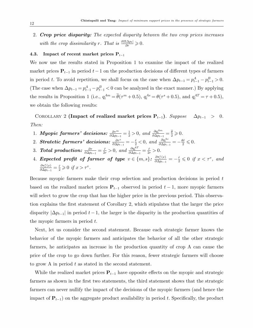
2. Crop price disparity: The expected disparity between the two crop prices increases

with the crop dissimilarity r. That is ∂|E∆pt|∂r> 0.

4.3. Impact of recent market prices Pt−1

We now use the results stated in Proposition 1 to examine the impact of the realized

market prices Pt−1 in period t−1 on the production decisions of different types of farmers

in period t. To avoid repetition, we shall focus on the case when ∆pt−1 = pAt−1− pBt−1 > 0.

(The case when ∆pt−1 = pAt−1−pBt−1 < 0 can be analyzed in the exact manner.) By applying

the results in Proposition 1 (i.e., qAmt = θ(τm + 0.5), qAst = θ(τ s + 0.5), and qATt = τ + 0.5),

we obtain the following results:

Corollary 2 (Impact of realized market prices Pt−1). Suppose ∆pt−1 > 0.

Then:

1. Myopic farmers’ decisions: ∂τm

∂∆pt−1= 1

2> 0, and

∂qAmt∂∆pt−1

= θ2> 0.

2. Stratetic farmers’ decisions: ∂τs

∂∆pt−1=− r

2< 0, and

∂qAst∂∆pt−1

=− θr26 0.

3. Total production: ∂τ∂∆pt−1

= r2r> 0, and

∂qATt∂∆pt−1

= r2r> 0.

4. Expected profit of farmer of type v ∈ {m,s}: ∂πvt (x)

∂∆pt−1= − r

26 0 if x < τ v, and

∂πvt (x)

∂∆pt−1= r

2> 0 if x> τ v.

Because myopic farmers make their crop selection and production decisions in period t

based on the realized market prices Pt−1 observed in period t− 1, more myopic farmers

will select to grow the crop that has the higher price in the previous period. This observa-

tion explains the first statement of Corollary 2, which stipulates that the larger the price

disparity |∆pt−1| in period t− 1, the larger is the disparity in the production quantities of

the myopic farmers in period t.

Next, let us consider the second statement. Because each strategic farmer knows the

behavior of the myopic farmers and anticipates the behavior of all the other strategic

farmers, he anticipates an increase in the production quantity of crop A can cause the

price of the crop to go down further. For this reason, fewer strategic farmers will choose

to grow A in period t as stated in the second statement.

While the realized market prices Pt−1 have opposite effects on the myopic and strategic

farmers as shown in the first two statements, the third statement shows that the strategic

farmers can never nullify the impact of the decisions of the myopic farmers (and hence the

impact of Pt−1) on the aggregate product availability in period t. Specifically, the product


with higher price in period t− 1 is always produced more in period t than the product

with lower price in period t− 1. Furthermore, according to the fourth statement of the

corollary, a higher value of ∆pt−1 causes a higher availability of crop A in period t and

hurts the expected profits of the farmers (both myopic and strategic) who grow crop A

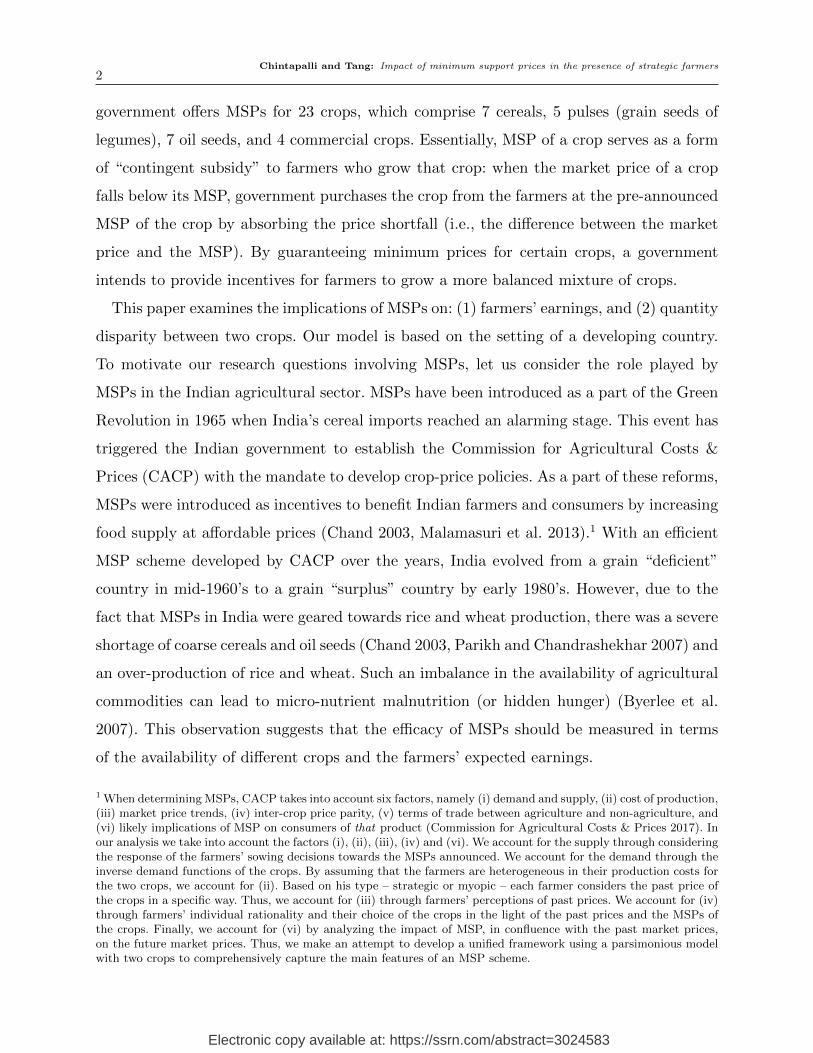
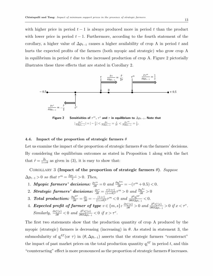
in equilibrium in period t due to the increased production of crop A. Figure 2 pictorially

illustrates these three effects that are stated in Corollary 2.

Figure 2 Sensitivities of τm, τs and τ in equilibrium to ∆pt−1. Note that

| ∂τs

∂∆pt−1|= | − r

2|< ∂τ

∂∆pt−1= r

2r< ∂τm

∂∆pt−1= 1

2.

4.4. Impact of the proportion of strategic farmers θ

Let us examine the impact of the proportion of strategic farmers θ on the farmers’ decisions.

By considering the equilibrium outcomes as stated in Proposition 1 along with the fact

that r= θr1+rθ

as given in (3), it is easy to show that:

Corollary 3 (Impact of the proportion of strategic farmers θ). Suppose

∆pt−1 > 0 so that τm = ∆pt−1

2> 0. Then,


∂θ= 0 and

∂qAmt∂θ

=−(τm + 0.5)< 0.

2. Strategic farmers’ decisions: ∂τs

∂θ= r(1+r)

(1+rθ)2 τm > 0 and

∂qAst∂θ

> 0

3. Total production:∂qATt∂θ

= ∂τ∂θ

=− (1+r)(1+rθ)2 τ

m < 0 and∂2qATt

∂θ∂∆pt−1< 0.


∂θ> 0 and

∂2πvt (x)

∂θ∂∆pt−1> 0 if x< τ v.

Similarly,∂πvt (x)

∂θ< 0 and

∂2πvt (x)

∂θ∂∆pt−1< 0 if x> τ v.

The first two statements show that the production quantity of crop A produced by the

myopic (strategic) farmers is decreasing (increasing) in θ. As stated in statement 3, the

submodularity of qATt (or τ) in (θ,∆pt−1) asserts that the strategic farmers “counteract”

the impact of past market prices on the total production quantity qATt in period t, and this

“counteracting” effect is more pronounced as the proportion of strategic farmers θ increases.


The fourth statement shows that the profit of a farmer (either myopic or strategic) growing

crop A (B) in equilibrium is increasing (decreasing) in θ. Moreover, the supermodularity

of πvt in (θ,∆pt−1) for x< τ v indicates that the negative impact of past price difference on

the farmers growing crop A is mitigated. In summary, the destabilizing effect of past prices

on the current expected equilibrium profits of the farmers is mitigated as the proportion

of strategic farmers increases.

To summarize, we have shown that past prices will have an impact on the farmers’ crop

selection and production decisions, product availability, and crops’ market prices in the

future periods. If a large portion of the farmers are myopic (i.e., θ is small) then the crop

with higher price in period t−1 (say, crop A) will be grown in abundance in period t. Due

to the high availability of crop A, its price in period t is very likely to be low, which hurts

the earnings of the those farmers who grow crop A. Consequently, high fluctuations in the

past crop prices will destabilize farmers’ profits in the current period. To safeguard the

earnings of the farmers, many governments in developing countries offer MSPs. However,

will MSPs create economic value to farmers? We examine this question in the next section.

5. Minimum Support Prices

We now extend our analysis presented in the last section to incorporate crop MSPs. To

begin, let mkt denote the MSP associated with crop k ∈ {A,B} in period t.4 Also, let pkmt

and pkst denote the effective market prices of crop k ∈ {A,B} in period t as “anticipated”

by myopic and strategic farmers, respectively.5 Because each myopic farmer anticipates

that the future selling price is equal to the most recently observed market price pkt−1,

myopic farmers will anticipate that pkmt = max{pkt−1,mkt } for crop k. However, because each

strategic farmer accounts for the actions of all the other farmers, each strategic farmer can

anticipate the effective market price in equilibrium based on its expected value so that

pkst =Eεkt max{pkt ,mkt } for crop k, where pkt is the actual market price as given in (1).

The decision making process employed by the farmers remains the same as explained in

Section 4, except that the anticipated prices pkmt and pkst are now replaced by pkmt and pkst

for k ∈ {A,B}. To ease our exposition and to identify the conditions under which offering

4 In general, the MSPs are announced before the crop sowing season; the farmers make their sowing decisions withthe complete knowledge of the MSPs and the price history of the crops.

5 To differentiate between the base case and the case when positive MSPs are offered, we useˆover the variables ofinterest in the latter case.


higher MSPs is detrimental to the farmers, we shall assume throughout this section that

the difference between the MSPs of two crops is bounded by 1 (i.e., |mAt − mB

t | < 1).

(However, except Propositions 4 and 5 that discuss possible disadvantages of MSPs, all

other results described in this section can be extended to MSPs such that |mAt −mB

t |> 1,

with additional notation.) We first characterize the unique equilibrium in the presence of

MSPs in Proposition 2, which is analogous to Proposition 1.

Proposition 2 (Equilibrium under MSPs). For any realized prices Pt−1 and for

any given MSPs (mAt ,m

Bt ), the equilibrium crop selection and production decisions of the

farmers in period t can be described as follows:

1. Myopic farmers’ decisions: The amount of crop A produced by myopic farmers is

given by qAmt = θ(τm + 0.5), where

τm =pAmt − pBmt

2∈ [−0.5,0.5], (6)

pkmt = max{pkt−1,mkt }, k ∈ {A,B}.

2. Strategic farmers’ decisions: The amount of crop A produced by strategic farmers

is given by qAst = θ(τ s + 0.5), where

τ s =−rτm−

[1

2(1 + rθ)

∫ mBt −φ−rτ

mAt −φ+rτ

F (ε)dε

]∈ [−0.5,0.5], (7)

r= θr1+rθ

and τ = θτ s + θτm.6

3. Total production: The total production of crop A is given by qATt = τ + 0.5 where

τ = θτ s + θτm ∈ [−0.5,0.5].

By using τm from (6) and the fact that τ = θτ s + θτm, we can obtain τ s by solving (7) as

an equation that involves τ s as the only variable. Once we determine τ s, we can retrieve

τ accordingly. Also, it can be shown that Proposition 2 reduces to Proposition 1 when

mAt =mB

t = 0.7

6 Note that (7) can be alternatively written as τs =−rτ− 12

∫mBt −φ−rτmAt −φ+rτ

F (ε)dε∈ [−0.5,0.5]. We will use either of these

two definitions of τs in our analysis, based on convenience.

7 First, to ensure that the crop prices are non-negative we require, pAt = E[pAt ] + εAt = φ− rτ + εAt > 0, which impliesthat εAt > −φ + rτ for all values of εAt . Second, by using the same arguement for crop B, we can conclude thatεBt >−φ−rτ for all values of εBt . Using these two observations and the fact that εAt and εBt follow the same distribution

F (·), we can conclude that F (ε) = 0 for all values of ε6max{−φ+rτ ,−φ−rτ}. Hence,∫mBt −φ−rτmAt −φ+rτ

F (ε)dε= 0 so that

τs is reduced to τs when mAt =mB

t = 0. Similarly, τm is reduced to τm and τ is reduced to τ when mAt =mB

t = 0.Hence, we can conclude that Proposition 2 reduces to Proposition 1 when mA

t =mBt = 0.


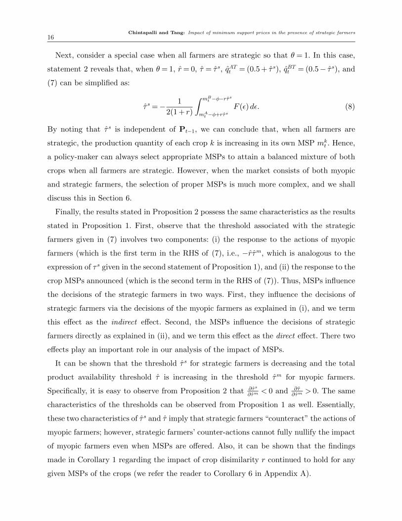
Next, consider a special case when all farmers are strategic so that θ = 1. In this case,

statement 2 reveals that, when θ= 1, r= 0, τ = τ s, qATt = (0.5 + τ s), qBTt = (0.5− τ s), and

(7) can be simplified as:

τ s =− 1

2(1 + r)

∫ mBt −φ−rτs

mAt −φ+rτsF (ε)dε. (8)

By noting that τ s is independent of Pt−1, we can conclude that, when all farmers are

strategic, the production quantity of each crop k is increasing in its own MSP mkt . Hence,

a policy-maker can always select appropriate MSPs to attain a balanced mixture of both

crops when all farmers are strategic. However, when the market consists of both myopic

and strategic farmers, the selection of proper MSPs is much more complex, and we shall

discuss this in Section 6.

Finally, the results stated in Proposition 2 possess the same characteristics as the results

stated in Proposition 1. First, observe that the threshold associated with the strategic

farmers given in (7) involves two components: (i) the response to the actions of myopic

farmers (which is the first term in the RHS of (7), i.e., −rτm, which is analogous to the

expression of τ s given in the second statement of Proposition 1), and (ii) the response to the

crop MSPs announced (which is the second term in the RHS of (7)). Thus, MSPs influence

the decisions of the strategic farmers in two ways. First, they influence the decisions of

strategic farmers via the decisions of the myopic farmers as explained in (i), and we term

this effect as the indirect effect. Second, the MSPs influence the decisions of strategic

farmers directly as explained in (ii), and we term this effect as the direct effect. There two

effects play an important role in our analysis of the impact of MSPs.

It can be shown that the threshold τ s for strategic farmers is decreasing and the total

product availability threshold τ is increasing in the threshold τm for myopic farmers.

Specifically, it is easy to observe from Proposition 2 that ∂τs

∂τm< 0 and ∂τ

∂τm> 0. The same

characteristics of the thresholds can be observed from Proposition 1 as well. Essentially,

these two characteristics of τ s and τ imply that strategic farmers “counteract” the actions of

myopic farmers; however, strategic farmers’ counter-actions cannot fully nullify the impact

of myopic farmers even when MSPs are offered. Also, it can be shown that the findings

made in Corollary 1 regarding the impact of crop disimilarity r continued to hold for any

given MSPs of the crops (we refer the reader to Corollary 6 in Appendix A).


In addition to the production quantities as stated in Proposition 2, we can compute the

farmers’ profits in equilibrium in the presence of MSPs (mAt ,m

Bt ). Analogous to (2), we can

express the expected profit of a farmer who is located at x and growing crop k ∈ {A,B}

as:

Πkt (x) = Eεkt

[max{pkt ,mk

t }]− ck(x)

=E[pkt ] +Eεkt[max{εt,mk

t −E[pkt ]}]− ck(x)

=E[pkt ] +(mkt −E[pkt ]

)F(mkt −E[pkt ]

)+

∫ ∞mkt−E[pkt ]

εf(ε)dε− ck(x). (9)

By considering (9), we can use the thresholds τm, τ s and τ stated in Proposition 2 along

with the production cost cA(x) = 0.5 + x and cB(x) = 0.5− x to determine the expected

profit in equilibrium for a farmer of type v ∈ {m,s} and who is located at x in period t as:

πvt (x) =

ΠAt (x) = E[pAt ] +

(mAt −E[pAt ]

)F(mAt −E[pAt ]

)+∫∞mAt −E[pAt ]

εf(ε)dε− (0.5 +x) if x6 τ v,

ΠBt (x) = E[pBt ] +

(mBt −E[pBt ]

)F(mBt −E[pBt ]

)+∫∞mBt −E[pBt ]

εf(ε)dε− (0.5−x) if x> τ v.

(10)

Also, by using statement 3 of Proposition 2 stating that qATt = 0.5 + τ and qBTt = 0.5− τ ,

we can apply (1) to determine the expected market price E[pAt ] and E[pBt ] in equilibrium

as a function of τ , which in turn depends on the MSPs via (7).

5.1. Impact of Pt−1 and θ

We now examine the impact of the most recently realized prices Pt−1 and the fraction

of strategic farmers θ on the equilibrium outcomes, which are as stated in Proposition 2,

in the presence of MSPs. Corollary 4, which is an analogue to Corollary 2, explains the

impact of Pt−1 on the equilibrium. For ease of exposition, we shall focus on crop A only.

Corollary 4 (Impact of the most recently realized prices Pt−1 under MSPs).

For any given MSPs (mAt ,m

Bt ), the impact of Pt−1 can be described as follows:


∂pAt−1> 0 and

∂qAmt∂pAt−1

> 0.


∂pAt−16 0 and ∂qAs

∂pAt−16 0.

3. Total production: ∂τ∂pAt−1

> 0 and ∂qAT

∂pAt−1> 0.


∂pAt−16 0 if x< τ v and

∂πvt (x)

∂pAt−1> 0 if

x> τ v.


It is easy to check that Corollary 4 resembles Corollary 2 (for any given pBt−1) even when

MSPs are present; hence, it can be interpreted in the same manner.

Next, we examine the impact of the proportion of strategic farmers θ on the equilibirium

outcomes. Corollary 5 is analogous to Corollary 3. However, because of the MSPs, the

analysis is more involved in the sense that the result hinges on the comparison between

the threshold τm, as defined in (6), and the threshold τ s0 , where τ s0 is the value of τ s (as

defined in (7)) evaluated at θ= 0. In other words, τ s0 ≡ τ s|θ=0 =−2rτm−∫mBt −φ−2rτm

mAt −φ+2rτmF (ε)dε

2.

It can shown that depending on the parameters and the distribution F (·), the difference

between τm and τ s0 can be positive or negative, but explicit conditions are not available.

Corollary 5 (Impact of strategic farmers under MSPs). For any given MSPs

(mAt ,m

Bt ), the impact of θ can be described as follows:


∂θ= 0 and ∂qAm

∂θ=−(τm + 0.5)6 0.


∂θ> 0 if and only if τm > τ s0 , and

∂qAst∂θ> 0.

3. Total production: ∂τ∂θ6 0, and

∂qATt∂θ6 0 if and only if τm > τ s0 .

4. Expected profit of farmer of type v ∈ {m,s}: If x6 τ v, then∂πvt (x)

∂θ> 0 if and only

if τm > τ s0 . Else, if x> τ v, then∂πvt (x)

∂θ6 0 if and only if τm > τ s0 .

When τm > τ s0 , the above corollary exhibits the same characteristics as Corollary 3 (for

the case when τm > τ s, which holds when the supposition pAt−1 > pBt−1 holds). Hence, it can

be interpreted in the same manner.

However, the above corollary exhibits opposite results when τm < τ s0 , where this condition

depends on the value of MSPs. This condition is not present in Corollary 3 because, in

the absence of MSPs, strategic farmers respond only to myopic farmers’ decisions that are

determined by the realized prices Pt−1. However, in the presence of MSPs, MSPs have a

direct impact (along with Pt−1) on the decisions of myopic farmers as described in (6).

Also, MSPs have both direct and indirect (via the actions of myopic farmers) impacts on

strategic farmers as described in (7), which makes the decisions of strategic farmers more

intricate. This observation calls for more attention to the analysis of the impact of MSPs

on farmers’ decisions. We explore this in the following section.


5.2. Impact of MSPs

We now examine the impact of MSPs on the farmer’s crop selection and production deci-

sions (again, we focus on crop A alone). In preparation, let us define the following two

bounds on the MSP of crop A.

mAt ≡mA

t (Pt−1,mBt ) = max{pAt−1,max{mB

t , pBt−1}− 1} and

mAt ≡mA

t (Pt−1,mBt ) = max{pAt−1,max{mB

t , pBt−1}+ 1}.

With these two bounds, MSP mAt is considered to be low when mA

t <mAt , moderate when

mAt 6m

At 6m

At , and high when mA

t >mAt . The two bounds mA

t and mAt are intended to

establish the necessary and sufficient conditions under which τm, which represents myopic

farmers’ crop selection decisions and that is defined in (6) in Proposition 2, is independent

of mAt , the MSP of crop A. It can be shown that τm is independent of mA

t if and only if

either mAt is low (i.e., mA

t 6mAt ) or mA

t is high (i.e., mAt >m

At ). 8 By doing this, we can

observe the impact of MSPs when (i) they have only the direct effect, and (ii) they have

both the direct and the indirect effects, on the decisions of strategic farmers given by τ s in

(7). By using the two bounds mAt and mA

t , along with the results as stated in Proposition

2, we obtain the following results:

Proposition 3 (Impact of MSPs on Equilibrium). For any given MSP mBt of

crop B, the MSP of crop A, mAt , affects the production decisions of myopic and strategic

farmers as follows:

1. Total production: The total availability of crop A is always increasing in the MSP

of A so that∂qATt∂mAt

= ∂τ∂mAt> 0.

2. Low MSP: When mAt 6m

At , then: (a) qAmt = θ

[pAt−1−max{mBt ,pBt−1}

2+ 1

2

]+

so that∂qAmt∂mAt

=

0, and (b)∂qAst∂mAt> 0.

3. High MSP: When mAt >m

At , then: (a) qAmt = θ so that

∂qAmt∂mAt

= 0, and (b)∂qAst∂mAt> 0.

4. Moderate MSP: When mAt <m

At <m

At , then: (a) qAmt ∈ (0, θ), and (b)

∂qAmt∂mAt

= θ2> 0.

8 Clearly, when mAt > m

At then pAt = max{mA

t , pAt−1} = mA

t > pBt + 1 so that all the myopic farmers grow crop A

and hence qAmt = θ(τm + 0.5) = θ(0.5 + 0.5) = θ, which is independent of mAt . On the other hand, if mA

t 6mAt then,

we consider two cases: (i) pAt−1 > max{mBt , p

Bt−1} − 1 and (ii) pAt−1 < max{mB

t , pBt−1} − 1. Under case (i), we have

mAt 6m

At = pAt−1 and |pAt−1 − pBmt |< 1 because mA

t −mBt |< 1 and |pAt−1 − pBt−1|< 1. Hence, τm =

pAt−1−pBmt

2>−0.5

so that qAmt = θ (τm + 0.5). Under case (ii), we have mAt 6m

At = max{mB

t , pBt−1} − 1, hence we have τm =−0.5 so

that qAmt = 0. Therefore, if mAt 6m

At , the total production quantity by myopic farmers can we written as qAmt =

θ

[pAt−1−max{mBt ,p

Bt−1}

2+ 1

2

]+

.


The first statement of Proposition 3 shows that the availability of a crop is always

increasing in the MSP offered for the crop. Due to this increase in the availability of the

crop, its market price drops as its MSP increases. Hence, the equilibrium expected market

price of crop A is decreasing in mAt (and increasing in mB

t with details omitted). Therefore,

to achieve a better balance of different crops, a policy-maker has to account for the effect

of MSP of one crop on the production of the other crop. Further, it is always possible to

obtain a desired production-mix of the crops using MSPs.9

Now, when MSP mAt is low (i.e., mA

t 6mAt ), the decisions of myopic farmers are inde-

pendent of mAt (as explained in footnote 8). Hence, when MSP mA

t is low, a slight increase

in the MSP mAt will not affect the sowing decisions of myopic farmers as stated in part (a)

of statement 2. Anticipating the myopic farmers’ sowing decisions, more strategic farmers

will grow crop A as MSP mAt increases. This explains part (b) of statement 2.

Next, when MSP mAt is high (i.e., mA

t >mAt ), all myopic farmers will grow crop A (as

explained in footnote 8). As such, increasing mAt will not increase myopic farmers’ pro-

duction of crop A any further. Anticipating the myopic farmers’ sowing decisions, more

strategic farmers will grow crop A as MSP mAt increases. This explains statement 3. Essen-

tially, the second and the third statements imply that, as long as myopic farmers are

“unaffected” by the increase in mAt , strategic farmers will increase their production of crop

A in order to benefit from the increase in mAt .

Finally, let us examine the fourth statement of Proposition 3 in which the MSP mAt

is moderate (i.e., mAt <mA

t <mAt ). In this case, it can be shown that the production of

crop A by the myopic farmers is strictly increasing in mAt (and decreasing in mB

t with

details omitted). As shown in the fourth statement, when the MSP is moderate so that

mAt < mA

t < mAt , more myopic farmers will grow crop A as the MSP mA

t increases (i.e.,

τm is increasing so that qAmt is increasing in the MSP mAt ). Anticipating myopic farmers’

behavior, strategic farmers make decisions in a more intricate manner, when the MSP mAt

is moderate. However, as it turns out, the amount of crop A produced by strategic farmers

qAst (or equivalently τ s) is not necessarily monotonic in the MSP mAt : offering a higher

9 To see why, suppose τtarget is the targeted production of crop A (so that 1− τtarget is the targeted production ofcrop B). Without loss of generality, assume that initially we set mA

t =mBt = 0 so that τ = τ , which is as defined in

Proposition 1. If τ = τ > τtarget then we can set mBt sufficiently high so that τ = τtarget is attained. This is possible

because from (7) we see that limmBt →∞τs = max{−∞,−0.5}=−0.5 and from (6) we see that limmBt →p

At−1+1 τ

m =

−0.5 so that limmBt →∞τ = limmBt →∞

{θτs + θτm}=−0.5. Likewise, on the other hand, if τ = τ < τtarget then we can

set mAt sufficiently high so that τ = τtarget is attained because it can be shown that limmAt →∞

τ = 0.5.


MSP for a crop can cause strategic farmers to produce less of the crop. We shall explore

this seemingly counter-intuitive result in more detail.

Due to the complexity of the analysis, we shall consider a special case when the market

uncertainty εkt ∼U [−δ, δ], k ∈ {A,B}, instead of a general probability distribution F (·). In

preparation, we let:

m= φ− δ(

1− r1 + r

)<φ= a− ρ+α

2.

Notice that m > 0 when a is sufficiently large and δ is sufficiently small. By considering m,

We obtain the following result:

Proposition 4 (Impact of MSPs on strategic farmers). Suppose the given MSP

mBt of crop B is such that mB

t > pBt−1. Then, for any moderately low MSP of A such

that mAt ∈

(mAt ,min{mB

t + 1, m}), there exists a threshold θ0 ≡ θ0(m

At ,m

Bt ) > 0 such that

∂τs

∂mAt< 0 if and only if 06 θ < θ0.10

While Proposition 4 is based on the assumption that the market uncertainty εkt ∼

U [−δ, δ], k ∈ {A,B}, the results stated in the proposition continue to hold for general

distribution. (Please see Proposition 6 in Appendix A for details.)

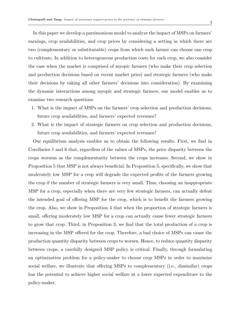
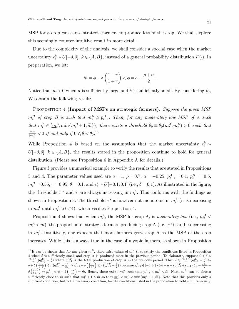
Figure 3 provides a numerical example to verify the results that are stated in Propositions

3 and 4. The parameter values used are a= 1, ρ= 0.7, α=−0.25, pAt−1 = 0.1, pBt−1 = 0.5,

mBt = 0.55, r= 0.95, θ= 0.1, and εkt ∼U [−0.1,0.1] (i.e., δ= 0.1). As illustrated in the figure,

the thresholds τm and τ are always increasing in mAt . This conforms with the findings as

shown in Proposition 3. The threshold τ s is however not monotonic in mAt (it is decreasing

in mAt until mA

t ≈ 0.74), which verifies Proposition 4.

Proposition 4 shows that when mAt , the MSP for crop A, is moderately low (i.e., mA

t <

mAt < m), the proportion of strategic farmers producing crop A (i.e., τ s) can be decreasing

in mAt . Intuitively, one expects that more farmers grow crop A as the MSP of the crop

increases. While this is always true in the case of myopic farmers, as shown in Proposition

10 It can be shown that for any given mBt , there exist values of mA

t that satisfy the conditions listed in Proposition4 when δ is sufficiently small and crop A is produced more in the previous period. To elaborate, suppose 0 < δ 6r(1+r)

2(qATt−1 − 1

2) where qATt−1 is the total production of crop A in the previous period. Then δ 6 r(1+r)

2(qATt−1 − 1

2)⇔

δ+δ(

1−r1+r

)6 r(qATt−1− 1

2

)⇒ εAt−1 +δ

(1−r1+r

)6 r(qATt−1− 1

2

)(because εAt−1 ∈ [−δ, δ])⇔ a−α−rqATt−1 + εt−1 <a− ρ+α

2−

δ(

1−r1+r

)⇔ pAt−1 < φ − δ

(1−r1+r

)= m. Hence, there exists mA

t such that pAt−1 < mAt < m. Next, mB

t can be chosen

sufficiently close to m such that mBt + 1 > m so that mA

t <mAt <min{mB

t + 1, m}. Note that this provides only asufficient condition, but not a necessary condition, for the conditions listed in the proposition to hold simultaneously.


Figure 3 τm, τs and τ as a function of MSP mAt .

3 when the MSP is moderately low, it is not true for strategic farmers when θ < θ0, as

shown in Proposition 4.

The rationale for this counter-intuitive result as stated in Proposition 4 is as follows.

Strategic farmers know that, when the MSP of crop A is moderate, more myopic farmers

will grow crop A as mAt increases. The resulting increase in production of crop A is substan-

tial when θ is small because, by using statement 1 of Proposition 2 (i.e., qAm = θ(τm+0.5)),

it is easy to see that: ∂qAm

∂mAt= θ ∂τ

m

∂mAt= θ

2when mA

t > pAt−1. This substantial increase in the

total production quantity qATt causes a significant drop in the price of crop A (and causes a

steep increase in the price of crop B). By anticipating myopic farmers’ behavior, strategic

farmers are better off by producing less of crop A and more of crop B. This explains the

seemingly counter-intuitive result that is stated in Proposition 4.

To summarize, we find that, when the MSP of crop A is moderately low, increasing the

MSP mAt can cause fewer strategic farmers to grow crop A (and more strategic farmers

to grow crop B). This seemingly counter-intuitive finding offers a hint regarding the con-

dition(s) under which offering MSP for a crop can hurt the earnings of farmers who grow

that crop. We shall explore this next.

5.3. Impact of MSPs on farmers’ profits

We now examine the impact of the MSP of crop A on the ex-ante expected profits of

farmers of each type v ∈ {m,s} as given by (10). By differentiating (10) with respect to

mAt and by using the fact that the expected market price E[pAt ] and E[pBt ] in equilibrium


depend on the MSPs via τ , we obtain:

∂πvt (x)

∂mAt

=

F(mAt −E[pAt ]

)+F

(mAt −E[pAt ]

)· ∂E[pAt ]

∂mAtif x6 τ v

F(mBt −E[pBt ]

)· ∂E[pBt ]

∂mAtif x> τ v

(11)

where∂E[pAt ]

∂mAt=−r ∂τ

∂mAt6 0 and

∂E[pBt ]

∂mAt= r ∂τ

∂mAt> 0. As before, we focus on the impact of the

MSP of crop A on the expected profits of the farmers. We introduce the following lemma.

Lemma 2 (Impact of MSPs on farmers’ profits). Consider a farmer of type v ∈{m,s} who is located at x∈ [−0.5,0.5].

1. Farmers growing crop B: If x> τ v, then∂πvt (x)

∂mAt> 0.

2. Low or high mAt on farmers growing crop A: If x6 τ v and mA

t is either low or

high (i.e., mAt <m

At or mA

t >mAt ), then

∂πvt (x)

∂mAt> 0.

The lemma explains the indirect benefit that mAt offers to the farmers growing crop B

(i.e., farmers who are located at x > τ v) in equilibrium. When mAt is increased, the total

availability of crop A (B) increases (decreases) according to statement 1 of Proposition

3. Hence, the expected market price of crop B increases, which will increase the expected

profit of those farmers who grow crop B in equilibrium. Furthermore, the lemma proves

that, as long as the decisions of the myopic farmers are not “affected” by mAt (i.e., mA

t is low

so that mAt 6m

At or mA

t is high so that mAt >m

At ), an increase in mA

t will always increase

the equilibrium expected profit of the farmers who grow crop A. This indicates that, when

the myopic farmers are not influenced by the changes in mAt , the strategic farmers will

make decisions in such a way that the expected profit of all the farmers growing crop A

will increase if mAt is increased.

It remains to analyze the impact of MSP of crop A on the farmers’ expected profits when

it is moderate (i.e., mAt <mA

t <mAt ). To simplify our analysis as before, let us consider

a special case when εAt and εBt are independent random variables that follow U [−δ, δ].Further, assume mk

t > pkt−1, k ∈ {A,B}, so that both the MSPs are effective. Also, we define

another threshold that will prove useful in our analysis. Let:

mA(mBt ) =

(r

r+ 2

)mBt +

2

r+ 2

[φ− δ

(2− r2 + r

)].

Akin to m as defined earlier, mA ≡ mA(mBt ) > 0 when φ is sufficiently large and δ is

sufficiently small. The following proposition shows that increasing the MSP of crop A can

hurt the expected profits of those farmers who grow crop A in equilibrium.


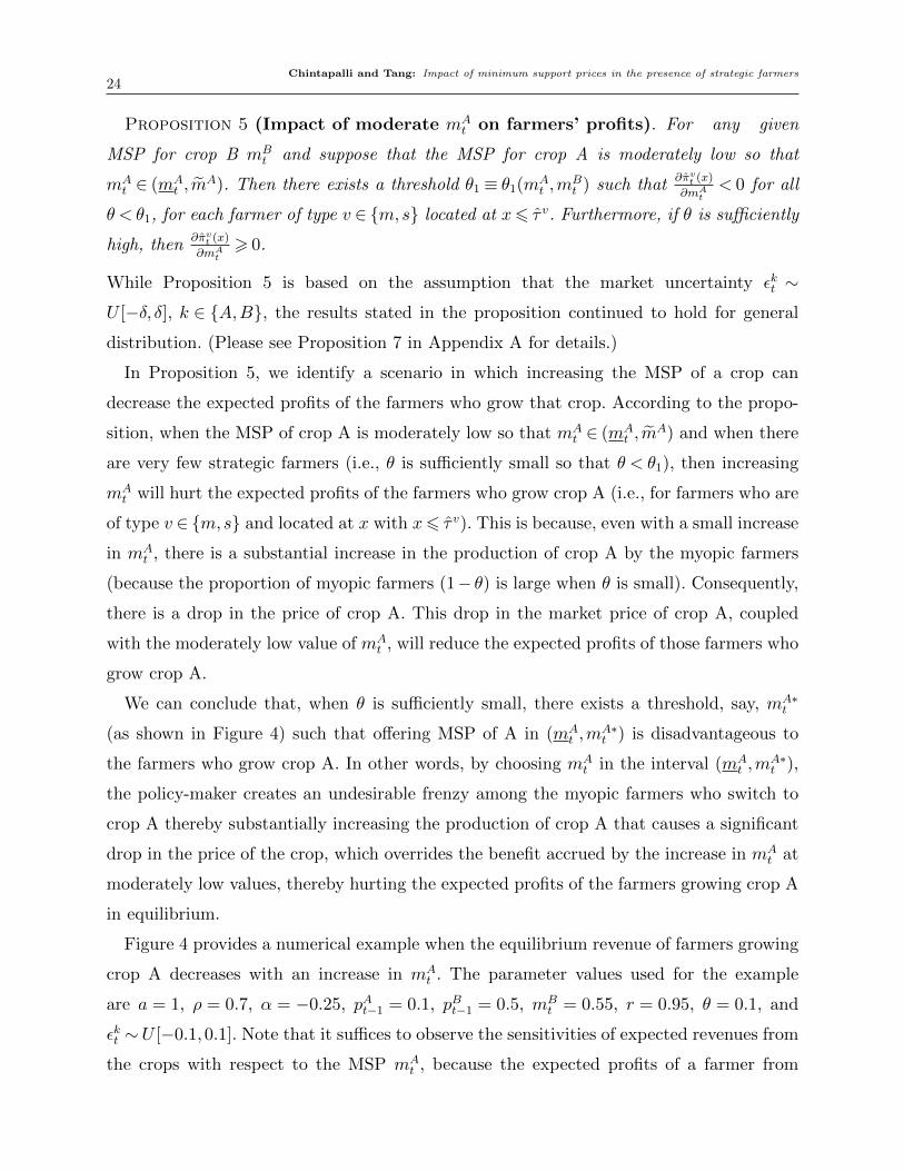
Proposition 5 (Impact of moderate mAt on farmers’ profits). For any given

MSP for crop B mBt and suppose that the MSP for crop A is moderately low so that

mAt ∈ (mA

t , mA). Then there exists a threshold θ1 ≡ θ1(m

At ,m

Bt ) such that

∂πvt (x)

∂mAt< 0 for all

θ < θ1, for each farmer of type v ∈ {m,s} located at x6 τ v. Furthermore, if θ is sufficiently

high, then∂πvt (x)

∂mAt> 0.

While Proposition 5 is based on the assumption that the market uncertainty εkt ∼U [−δ, δ], k ∈ {A,B}, the results stated in the proposition continued to hold for general

distribution. (Please see Proposition 7 in Appendix A for details.)

In Proposition 5, we identify a scenario in which increasing the MSP of a crop can

decrease the expected profits of the farmers who grow that crop. According to the propo-

sition, when the MSP of crop A is moderately low so that mAt ∈ (mA

t , mA) and when there

are very few strategic farmers (i.e., θ is sufficiently small so that θ < θ1), then increasing

mAt will hurt the expected profits of the farmers who grow crop A (i.e., for farmers who are

of type v ∈ {m,s} and located at x with x6 τ v). This is because, even with a small increase

in mAt , there is a substantial increase in the production of crop A by the myopic farmers

(because the proportion of myopic farmers (1− θ) is large when θ is small). Consequently,

there is a drop in the price of crop A. This drop in the market price of crop A, coupled

with the moderately low value of mAt , will reduce the expected profits of those farmers who

grow crop A.

We can conclude that, when θ is sufficiently small, there exists a threshold, say, mA∗t

(as shown in Figure 4) such that offering MSP of A in (mAt ,m

A∗t ) is disadvantageous to

the farmers who grow crop A. In other words, by choosing mAt in the interval (mA

t ,mA∗t ),

the policy-maker creates an undesirable frenzy among the myopic farmers who switch to

crop A thereby substantially increasing the production of crop A that causes a significant

drop in the price of the crop, which overrides the benefit accrued by the increase in mAt at

moderately low values, thereby hurting the expected profits of the farmers growing crop A

in equilibrium.

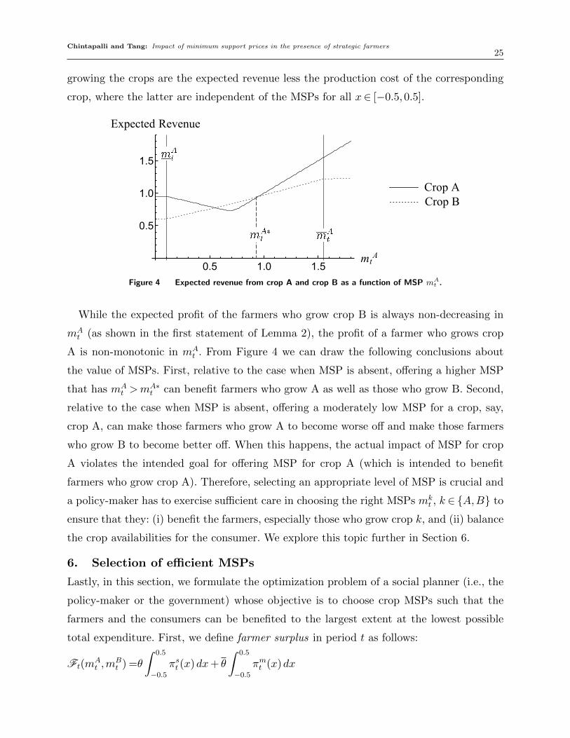
Figure 4 provides a numerical example when the equilibrium revenue of farmers growing

crop A decreases with an increase in mAt . The parameter values used for the example

are a = 1, ρ = 0.7, α = −0.25, pAt−1 = 0.1, pBt−1 = 0.5, mBt = 0.55, r = 0.95, θ = 0.1, and

εkt ∼U [−0.1,0.1]. Note that it suffices to observe the sensitivities of expected revenues from

the crops with respect to the MSP mAt , because the expected profits of a farmer from


growing the crops are the expected revenue less the production cost of the corresponding

crop, where the latter are independent of the MSPs for all x∈ [−0.5,0.5].

Figure 4 Expected revenue from crop A and crop B as a function of MSP mAt .

While the expected profit of the farmers who grow crop B is always non-decreasing in

mAt (as shown in the first statement of Lemma 2), the profit of a farmer who grows crop

A is non-monotonic in mAt . From Figure 4 we can draw the following conclusions about

the value of MSPs. First, relative to the case when MSP is absent, offering a higher MSP

that has mAt >m

A∗t can benefit farmers who grow A as well as those who grow B. Second,

relative to the case when MSP is absent, offering a moderately low MSP for a crop, say,

crop A, can make those farmers who grow A to become worse off and make those farmers

who grow B to become better off. When this happens, the actual impact of MSP for crop

A violates the intended goal for offering MSP for crop A (which is intended to benefit

farmers who grow crop A). Therefore, selecting an appropriate level of MSP is crucial and

a policy-maker has to exercise sufficient care in choosing the right MSPs mkt , k ∈ {A,B} to

ensure that they: (i) benefit the farmers, especially those who grow crop k, and (ii) balance

the crop availabilities for the consumer. We explore this topic further in Section 6.

6. Selection of efficient MSPs

Lastly, in this section, we formulate the optimization problem of a social planner (i.e., the

policy-maker or the government) whose objective is to choose crop MSPs such that the

farmers and the consumers can be benefited to the largest extent at the lowest possible

total expenditure. First, we define farmer surplus in period t as follows:

Ft(mAt ,m

Bt ) =θ

∫ 0.5

−0.5

πst (x)dx+ θ

∫ 0.5

−0.5

πmt (x)dx


=θ

[∫ τs

−0.5

(E[max{pAt ,mA

t }]− (x+ 0.5)

)dx+

∫ 0.5

τs

(E[max{pBt ,mB

t }]− (0.5−x)

)dx

]+ θ

[∫ τm

−0.5

(E[max{pAt ,mA

t }]− (x+ 0.5)

)dx+

∫ 0.5

τm

(E[max{pBt ,mB

t }]− (0.5−x)

)dx

],

where pAt =E[pAt ]+ εAt = φ− rτ + εAt , pBt =E[pBt ]+ εBt = φ+ rτ + εBt and τ = θτ s+θτm, as in

Proposition 2. Second, We capture the disutility of the consumers through the imbalance

of crop availability as follows:

Ct(mAt ,m

Bt ) =−

(qATt − qBTt

)2=−4τ 2.

Third, the total expected expenditure incurred by the policy-maker by setting MSPs mAt

and mBt is given by:

Kt(mAt ,m

Bt ) =qATt ·E[mA

t − pAt ]+ + qBTt ·E[mBt − pBt ]+

=(τ + 0.5)E[mAt −φ+ rτ − εAt ]+ + (0.5− τ)E[mB

t −φ− rτ − εBt ]+,

because government has to bear an expected expenditure of E[mkt −pkt ]+ for all the quantity

of qkTt of crop k ∈ {A,B} produced. The quantity qkTt is as given in Proposition 2.

Using Ft, Ct and Kt, we can define the social welfare (maximization) problem (SWPt)

in period t as below:

SWPt : maxmAt ,m

Bt

Wt(mAt ,m

Bt ) = {λFt(m

At ,m

Bt ) + (1−λ)Ct(m

At ,m

Bt )}− ηKt(m

At ,m

Bt )

such that 06mkt 6M,k ∈ {A,B},

Kt(mAt ,m

Bt )6B,

where λ ∈ (0,1) and (1− λ) ∈ (0,1) are the exogenous weights associated by the policy-

maker to farmers’ welfare and consumers’ welfare, respectively, η is the sensitivity of the

policy-maker (or the government) to its expenditure, M is the maximum limit of the MSP

to be awarded to a crop, and B is a bound on the expected expenditure to be incurred

(we can consider the constraint Kt(mAt ,m

Bt )6B as a budget constraint).

Having analyzed the impact of MSPs chosen by a policy-maker on farmers’ crop selection

and production decisions in the earlier section, we now focus on the effect of crop dissimi-

larity r (i.e., substitutability or complementarity) on the optimal choice of crop MSPs and

crop balance. Offering crop MSPs without understanding the degree of complementarity


(or substitutability) between the crops being supported by the MSPs can destabilize the

availability of those crops to the consumers. For instance, MSPs focused on wheat and

rice (which are substitutes) caused a severe shortage of coarse cereals and oil seeds and

an over-production of rice and wheat in the Indian economy (Chand 2003, Parikh and

Chandrashekhar 2007). Hence, we note that it is important to explore the impact of r,

which measures the “dissimilarity” between the two crops, on the choice of MSPs and the

consequent production decisions of farmers.

Given the complexity of the above problem, we solve it numerically and draw some

insights. The parameter values used in our numerical example are a= 1, ρ= 0.7, pAt−1 = 0.1,

pBt−1 = 0.9, θ = 0.1, η = 0.3, B = 0.2, M = 1 and εkt ∼ U [−0.1,0.1]. We take the “weight”

λ = 0.1,0.5,1, which correspond to low, medium and high values, respectively. In our

discussion we focus on the impact of crop dissimilarity (r) on the optimal choice of MSPs.

We change r by varying α while retaining ρ constant (i.e., ρ= 0.7).

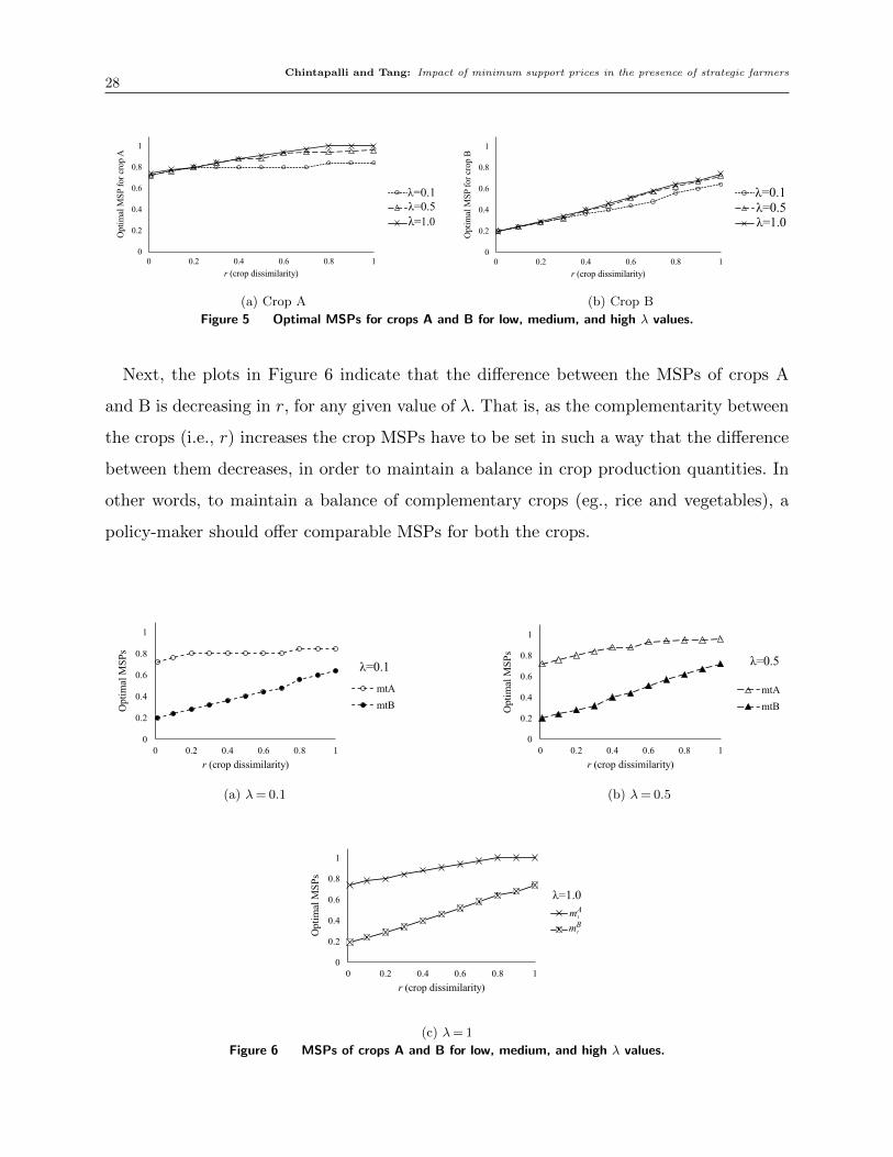
As shown in Figure 5, the optimal value of MSP for crop A is higher than that for

crop B, for each value of λ, because our example is based on the case when the previous

period price of crop A is lower than that of crop B (i.e., 0.1 = pAt−1 < pBt−1 = 0.9). Because

of this past price differential, more myopic farmers choose to grow crop B and so a larger

MSP should be offered for crop A in order to entice a few of these farmers to switch to

growing crop A from growing crop B. Furthermore, we notice that the optimal MSPs of

the crops are increasing in r, which can be explained as follows. When r increases (i.e., α

decreases while ρ is left unchanged), the expected prices of the crops increase, for any given

production quantities of the crops.11 Hence it is less likely that the realized market prices

are lower than the crop MSPs. As such, the government can afford to increase the MSPs

in order to benefit the farmers. Thus, for any given budget, government will be able to

offer higher MSPs for complementary crops (like rice/wheat and pulses/vegetables) than

for substitutable crops (like rice and wheat).

Furthermore, when a policy-maker gives higher importance to the welfare of the farmers

(i.e., as λ increases), the crop MSPs also increase, because, when appropriately chosen,

higher MSPs improve farmers’ revenues. The case when λ= 1 corresponds to the extreme

case when a policy-maker is concerned only about the welfare of the farmers but not at all

about the welfare of the consumers.

11 Note that by differentiating (1) with respect to α, we obtain for k ∈ {A,B} that∂E[pkt ]

∂α=−qjTt 6 0, j 6= k.


(a) Crop A (b) Crop B

Figure 5 Optimal MSPs for crops A and B for low, medium, and high λ values.

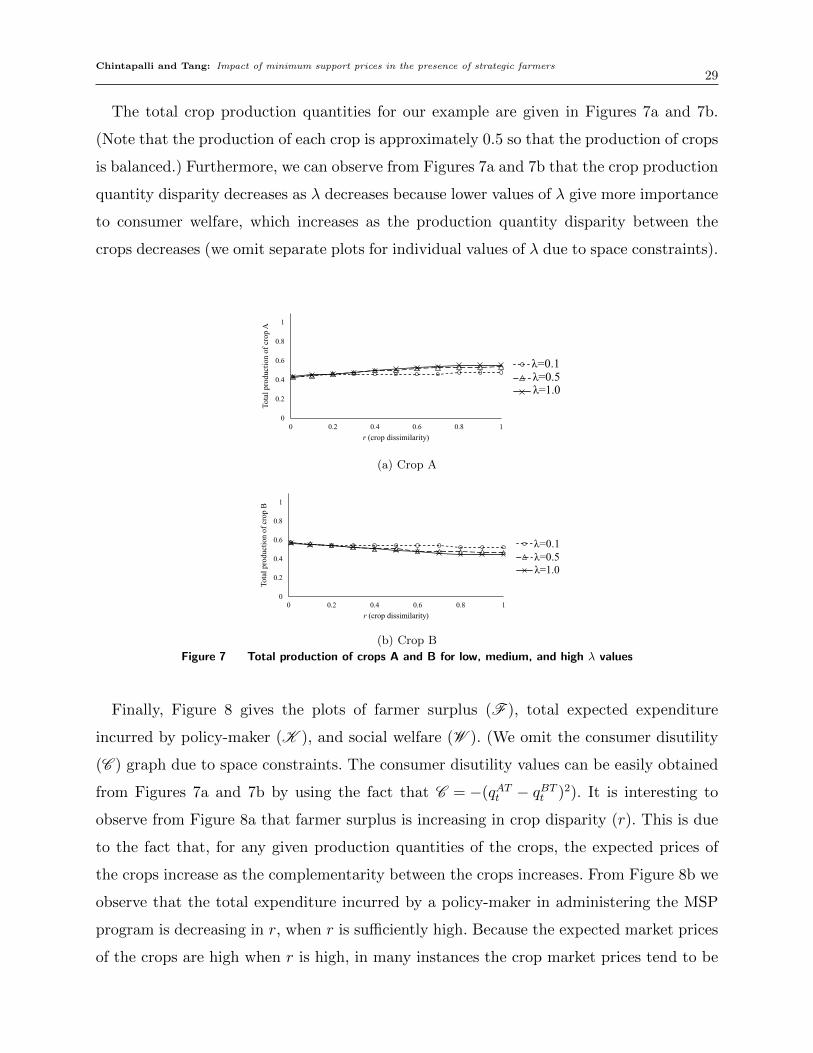
Next, the plots in Figure 6 indicate that the difference between the MSPs of crops A

and B is decreasing in r, for any given value of λ. That is, as the complementarity between

the crops (i.e., r) increases the crop MSPs have to be set in such a way that the difference

between them decreases, in order to maintain a balance in crop production quantities. In

other words, to maintain a balance of complementary crops (eg., rice and vegetables), a

policy-maker should offer comparable MSPs for both the crops.

(a) λ= 0.1 (b) λ= 0.5

(c) λ= 1

Figure 6 MSPs of crops A and B for low, medium, and high λ values.


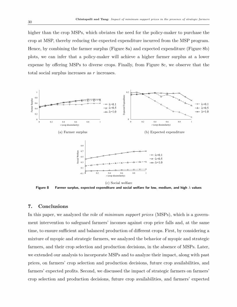
The total crop production quantities for our example are given in Figures 7a and 7b.

(Note that the production of each crop is approximately 0.5 so that the production of crops

is balanced.) Furthermore, we can observe from Figures 7a and 7b that the crop production

quantity disparity decreases as λ decreases because lower values of λ give more importance

to consumer welfare, which increases as the production quantity disparity between the

crops decreases (we omit separate plots for individual values of λ due to space constraints).

(a) Crop A

(b) Crop B

Figure 7 Total production of crops A and B for low, medium, and high λ values

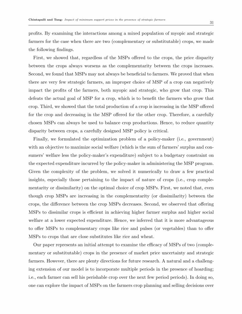
Finally, Figure 8 gives the plots of farmer surplus (F ), total expected expenditure

incurred by policy-maker (K ), and social welfare (W ). (We omit the consumer disutility

(C ) graph due to space constraints. The consumer disutility values can be easily obtained

from Figures 7a and 7b by using the fact that C = −(qATt − qBTt )2). It is interesting to

observe from Figure 8a that farmer surplus is increasing in crop disparity (r). This is due

to the fact that, for any given production quantities of the crops, the expected prices of

the crops increase as the complementarity between the crops increases. From Figure 8b we

observe that the total expenditure incurred by a policy-maker in administering the MSP

program is decreasing in r, when r is sufficiently high. Because the expected market prices

of the crops are high when r is high, in many instances the crop market prices tend to be


higher than the crop MSPs, which obviates the need for the policy-maker to purchase the

crop at MSP, thereby reducing the expected expenditure incurred from the MSP program.

Hence, by combining the farmer surplus (Figure 8a) and expected expenditure (Figure 8b)

plots, we can infer that a policy-maker will achieve a higher farmer surplus at a lower

expense by offering MSPs to diverse crops. Finally, from Figure 8c, we observe that the

total social surplus increases as r increases.

(a) Farmer surplus (b) Expected expenditure

(c) Social welfare

Figure 8 Farmer surplus, expected expenditure and social welfare for low, medium, and high λ values

7. Conclusions

In this paper, we analyzed the role of minimum support prices (MSPs), which is a govern-

ment intervention to safeguard farmers’ incomes against crop price falls and, at the same

time, to ensure sufficient and balanced production of different crops. First, by considering a

mixture of myopic and strategic farmers, we analyzed the behavior of myopic and strategic

farmers, and their crop selection and production decisions, in the absence of MSPs. Later,

we extended our analysis to incorporate MSPs and to analyze their impact, along with past

prices, on farmers’ crop selection and production decisions, future crop availabilities, and

farmers’ expected profits. Second, we discussed the impact of strategic farmers on farmers’

crop selection and production decisions, future crop availabilities, and farmers’ expected


profits. By examining the interactions among a mixed population of myopic and strategic

farmers for the case when there are two (complementary or substitutable) crops, we made

the following findings.

First, we showed that, regardless of the MSPs offered to the crops, the price disparity

between the crops always worsens as the complementarity between the crops increases.

Second, we found that MSPs may not always be beneficial to farmers. We proved that when

there are very few strategic farmers, an improper choice of MSP of a crop can negatively

impact the profits of the farmers, both myopic and strategic, who grow that crop. This

defeats the actual goal of MSP for a crop, which is to benefit the farmers who grow that

crop. Third, we showed that the total production of a crop is increasing in the MSP offered

for the crop and decreasing in the MSP offered for the other crop. Therefore, a carefully

chosen MSPs can always be used to balance crop productions. Hence, to reduce quantity

disparity between crops, a carefully designed MSP policy is critical.

Finally, we formulated the optimization problem of a policy-maker (i.e., government)

with an objective to maximize social welfare (which is the sum of farmers’ surplus and con-

sumers’ welfare less the policy-maker’s expenditure) subject to a budgetary constraint on

the expected expenditure incurred by the policy-maker in administering the MSP program.

Given the complexity of the problem, we solved it numerically to draw a few practical

insights, especially those pertaining to the impact of nature of crops (i.e., crop comple-

mentarity or dissimilarity) on the optimal choice of crop MSPs. First, we noted that, even

though crop MSPs are increasing in the complementarity (or dissimilarity) between the

crops, the difference between the crop MSPs decreases. Second, we observed that offering

MSPs to dissimilar crops is efficient in achieving higher farmer surplus and higher social

welfare at a lower expected expenditure. Hence, we inferred that it is more advantageous

to offer MSPs to complementary crops like rice and pulses (or vegetables) than to offer

MSPs to crops that are close substitutes like rice and wheat.

Our paper represents an initial attempt to examine the efficacy of MSPs of two (comple-

mentary or substitutable) crops in the presence of market price uncertainty and strategic

farmers. However, there are plenty directions for future research. A natural and a challeng-

ing extension of our model is to incorporate multiple periods in the presence of hoarding;

i.e., each farmer can sell his perishable crop over the next few period periods). In doing so,

one can explore the impact of MSPs on the farmers crop planning and selling decisions over


time. Another direction of future research is to examine the economic value of agricultural

advisory services to farmers. Specifically, one can analyze the impact of long-term farming

assistance programs that can enable farmers to take more strategic production decisions.

Such a study will provide insights on the design and choice of such long-term programs

vis-a-vis short-term (contingent) subsidy programs such as MSPs.

References

Alizamir S, Iravani F, Mamani H (2015) Price vs. revenue protection: An analysis of government subsidies

in the agriculture industry. Technical report, Working paper.

An J, Cho SH, Tang CS (2015) Aggregating smallholder farmers in emerging economies. Production and

Operations Management 24(9):1414–1429.

Byerlee D, Janvry AD, Sadoulet E, Townsend R, Klytchnikova I (2007) World development

report 2008 : Agriculture for development. URL http://documents.worldbank.org/curated/en/

587251468175472382/World-development-report-2008-agriculture-for-development.

Chand R (2003) Minimum support price in agriculture: Changing requirements. Economic and Political

Weekly 3027–3028.

Chen YJ, Tang CS (2015) The economic value of market information for farmers in developing economies.

Production and Operations Management 24(9):1441–1452.

Chhatre A, Devalkar S, Seshadri S, Ramaswami B (2016) Crop diversification = Profit and Risk: The Role

of Intermediaries (Presented at the 4th ISB – POMS workshop, Indian School of Business, Hyderabad,

India).

Commission for Agricultural Costs & Prices (2017) Determinants of MSP. URL http://cacp.dacnet.nic.

in, Ministry of Agriculture & Farmers Welfare, Government of India, Accessed July 3, 2017.

Dantwala M (1967) Incentives and disincentives in Indian agriculture. Indian Journal of Agricultural Eco-

nomics 22(2):1.

Dawande M, Gavirneni S, Mehrotra M, Mookerjee V (2013) Efficient distribution of water between head-

reach and tail-end farms in developing countries. Manufacturing & Service Operations Management

15(2):221–238.

Federgruen A, Lall U, Simsek AS (2015) Supply chain analysis of contract farming. Technical report, Working

paper.

Fox KA (1956) The contribution of farm price support programs to general economic stability. Policies to

Combat Depression, 295–356 (NBER).

Guda H, Rajapakshe T, Dawande M, Janakiraman G (2016) Agricultural support prices in developing

economies: Operational analysis and its use in policy making. Technical report, Working paper.


Hu M, Liu Y, Wang W (2016) Altruistic rationality: The value of strategic farmers, social entrepreneurs and

for-profit firms in crop planting decisions .

Huh WT, Athanassoglou S, Lall U (2012) Contract farming with possible reneging in a developing country:

Can it work? IIMB Management Review 24(4):187–202.

Huh WT, Lall U (2013) Optimal crop choice, irrigation allocation, and the impact of contract farming.

Production and Operations Management 22(5):1126–1143.

Kazaz B, Webster S (2011) The impact of yield-dependent trading costs on pricing and production planning

under supply uncertainty. Manufacturing & Service Operations Management 13(3):404–417.

Liao CN, Chen YJ, Tang CS (2017) Information provision policies for improving farmer welfare in devel-

oping countries: Heterogeneous farmers and market selection. Manufacturing & Service Operations

Management .

Malamasuri K, B S, Parmar P, Malve S (2013) A historical perspective for minimum support price of

agriculture crops. Kisan World – A Journal of Agriculture and Rural Development 40(12):46–48.

Parikh J, Chandrashekhar S (2007) Extension of msp: Fiscal and welfare implications. A Study for the

Planning Commission [of India] by Integrated Action and Research for Development .

Parker C, Ramdas K, Savva N (2016) Is it enough? evidence from a natural experiment in India’s agriculture

markets. Management Science 62(9):2481–2503.

Spitze R (1978) The food and agriculture act of 1977: issues and decisions. American Journal of Agricultural

Economics 60(2):225–235.

Subbarao D, et al. (2011) The challenge of food inflation. Technical report.

Tang CS, Wang Y, Zhao M (2015) The implications of utilizing market information and adopting agricultural

advice for farmers in developing economies. Production and Operations Management 24(8):1197–1215.

Thorbecke E (1982) Agricultural sector analysis and models in developing countries. Number 5 (Food &

Agriculture Org.).

Tripathi AK, et al. (2013) Agricultural price policy, output, and farm profitabilityexamining linkages during

post-reform period in India. Asian Journal of Agriculture and Development 10(1):91–111.

Appendix A: Supplementary and Additional Results

Corollary 6 (Impact of crop dissimilarity). For a given pair of MSPs (mAt ,m

Bt ) the following state-

ments hold:

1. Crop availability disparity: The disparity between the total production quantities of the crops

decreases with r if there are strategic farmers. That is ∂|∆qt|∂r

< 0 if θ > 0 where ∆qt = qATt − qBTt . If

θ= 0, then ∂|∆qt|∂r

= 0.

2. Crop price disparity: However, the expected disparity between the two crop prices increases with the

crop dissimilarity r. That is ∂|E∆pt|∂r

> 0.


Proposition 6 (Some strategic farmers may forgo low MSPs). Let ˜m be the unique value of mAt

satisfying the equation F (mAt −φ+ rτm) = r

2+r. Then for each mA

t such that mAt <mA

t < min{mAt , ˜m}12,

there exists a θ0 such that ∂τs

∂mAt6 0 for all θ < θ0. Further, if θ is sufficiently high then ∂τs

∂mAt> 0 always (i.e.,

limθ→1∂τs

∂mAt> 0 always).

Proposition 7 (Effect of moderate MSPs). Let ˜m be the unique value of mAt satisfying the equation

F (mAt −φ+ rτm) = r

2+r. Then for each mA

t such that mAt <mA

t <min{mAt , ˜m}13, there exists a threshold

θ1 such that∂πvt (x)

∂mAt6 0 for all θ < θ1, for each farmer of type v ∈ {m,s} located at x6 τ v. Further, if θ is

sufficiently high then∂πvt (x)

∂mAt> 0 always (i.e., limθ→1

∂πAt∂mAt> 0 always).

Appendix B: Proofs

Proof of Lemma 1: First, we note that

|ξt|6 2β(1− r)⇒−2β(1− r)6 ξt 6 2β(1− r)⇒{−2β 6 ξt− 2rβ} ∧ {ξt + 2rβ 6 2β}

⇒−2β 6−2rβ+ ξt 6 pAt − pBt 6 2rβ+ ξt 6 2β⇒ |pAt − pBt |6 2β.

Hence,

|pAt − pBt |> 2β⇒ |ξt|> 2β(1− r)

⇔ P(|pAt − pBt |> 2β

)6 P (|ξt|> 2β(1− r))6

(σ√

2β(1− r)

)2

,

where the last inequality is obtained by using Chebyshev’s inequality. �

Proof of Lemma 2: The first statement is proved by using (11) and the fact that∂E[pBt ]

∂mAt= r ∂τ

∂mAt> 0.

For the second statement, by substituting (23) in (11) and simplifying, we obtain that for every x6 τ v,

v ∈ {m,s},

∂πvt (x)

∂mAt

=2F (mA

t −φ+ rτ) + rθF (mAt −φ+ rτ)F (mB

t −φ− rτ)− 2rθ F (mAt −φ+ rτ) ∂τm

∂mAt

2 + rθ(F (mA

t −φ+ rτ) +F (mBt −φ− rτ)

) (12)

which is non-negative if ∂τm

∂mAt= 0. Hence, by using Proposition 3 we obtain the desired result. �

Proof of Proposition 1:

1. The myopic farmers anticipate the price in period t to be the same as the price in period t− 1. A

farmer produces crop A as long as the anticipated benefit from crop A is more than that from crop

B, otherwise the farmer produces crop B (by Assumption 1). Therefore, the fraction of myopic farmers

growing crop A is then given by:

P(pAmt−1− cA(x)> pBmt−1− cB(x)

)= P

(pAmt−1−

(x+

1

2

)> pBmt−1−

(1

2−x))

= P(x6

pAmt−1− pBmt−1

2

)=

(pAmt−1− pBmt−1

2

)+ 0.5 (13)

sincepAmt−1−p

Bmt−1

2∈ [−0.5,0.5] (by Assumption 2). Thus, we obtain the threshold value as τm =

pAmt−1−pBmt−1

2.

12 Note that if ˜m<mAt then the range of interest is empty. Hence, this condition is likely to be encountered when

pAt−1 is sufficiently low.

13 Note that if ˜m<mAt then the range of interest is empty. Hence, this condition is likely to be encountered when

pAt−1 is sufficiently low.


2. The strategic farmers on the other hand are forward-looking and hence anticipate the market price

in period t by taking into account the total availability of the crops, which takes into account the

behaviors of the myopic farmers and the other strategic farmers. Hence, by using the principle of rational

expectations, the fraction of the strategic farmers growing crop A is given by:

P(E[pAt ]− cA(x)>E[pBt ]− cB(x)

)= P

(x6

E[pAt ]−E[pBt ]

2

). (14)

From (1), and the fact that qBTt = 1− qATt we obtain

E[pAt ] = a−α− rqATt and E[pBt ] = a− ρ+ rqATt ⇒E[pAt ]−E[pBt ] = r(1− 2qATt )∈ (−r, r)⊂ (−1,1),

where qATt ∈ [0,1] is the total production quantity of crop A. Therefore, from (14) we obtain the

threshold τ s as:

τ s =E[pAt ]−E[pBt ]

2=r(1− 2qATt )

2. (15)

and the total production quantity of crop A by strategic farmers is qAst = θ(τ s + 0.5). Further, using

the fact that qATt = qAst + qAmt = θτ s + θτm + 0.5 and substituting it in (15) we obtain:

τ s =

(−rθ

1 + rθ

)τm =−rτm.

Note that |τ s|= |r||τm|< |τm| ⇒ τ s ∈ [−0.5,0.5] since r < 1 by Assumption 2.

3. The total availability of crop A is given by

qATt = qAst + qAmt = θτ s + θτm + 0.5 = τ + 0.5, (16)

and by using (15), we obtain τ = θτm

1+rθ. Note that |τ |= | r

r||τm|< |τm| ⇒ τ ∈ [−0.5,0.5] since r < r.


1. The fraction of myopic farmers sowing crop A is given by:

P(pAmt − cA(x)> pBmt − cB(x)

)= P

(x6

pAmt − pBmt2

).

Since |pAt −pBt |< 1 and |mAt −mB

t |< 1 by assumptions, we obtain |pAmt − pBmt |< 1 so that the threshold

value τm is given by τm =pAmt −pBmt

2∈ [−0.5,0.5]. The total quantity of crop A produced by myopic

farmers is given by qAmt = θ(τm + 0.5).

2. On the other hand, the price anticipated by the strategic farmers for crop k ∈ {A,B} is given by

pkst =Eεt max{pkt ,mkt } where pkt =E[pkt ] + εt. Hence, the fraction of strategic farmers growing crop A is

given by:

P(pAst − cA(x)> pBst − cB(x)

)= P

(x6

pAst − pBst2

). (17)

Using the fact that pkst =E[pkt ] +Eεt max{εt,mkt −E[pkt ]}, we can write

pAst − pBst =E[pAt ]−E[pBt ]−∫ ∞mAt −E[pAt ]

F (ε)dε+

∫ ∞mBt −E[pBt ]

F (ε)dε

=E[pAt ]−E[pBt ]−∫ mBt −E[pBt ]

mAt −E[pAt ]

F (ε)dε. (18)


We know that E[pAt ]−E[pBt ] = r(1−2qATt )∈ (−1,1), where qATt is the total availability of crop A. Hence,

(18) can we written as:

pAst − pBst =E[pAt ]−E[pBt ]−∫ mBt −E[pBt ]

mAt −E[pAt ]

F (ε)dε. (19)

For any given set of MSPs (mAt ,m

Bt ), we have exactly one of these three cases to hold: (i) E[pAt ]−E[pBt ]>

mAt −mB

t , or (ii) E[pAt ]− E[pBt ] <mAt −mB

t , or (iii) E[pAt ]− E[pBt ] = mAt −mB

t . When (iii)holds, then

trivially pAst − pBst = E[pAt ]−E[pBt ] ∈ (−1,1). Hence, it remains to check if pAst − pBst ∈ (−1,1) for cases

(i) and (ii).

In case (i), we note that


mAt −E[pAt ]

F (ε)dε6E[pAt ]−E[pBt ]< 1, and


mAt −E[pAt ]

F (ε)dε>E[pAt ]−E[pBt ]−{mBt −E[pBt ]− (mA

t −E[pBt ] + 2rτ)}

=mAt −mB

t >−1.

In case (ii), we get

pAst − pBst =E[pAt ]−E[pBt ] +

∫ mAt −E[pAt ]

mBt −E[pBt ]

F (ε)dε>E[pAt ]−E[pBt ]>−1, and

pAst − pBst =E[pAt ]−E[pBt ] +

∫ mAt −E[pAt ]

mBt −E[pBt ]

F (ε)dε6−2rτ + {mAt −E[pBt ] + 2rτ − (mB

t −E[pBt ])}

=mAt −mB

t < 1.

Hence, if |mAt −mB

t |< 1 then pAst − pBst ∈ (−1,1) always and so we obtain the threshold τ s as

τ s =pAst − pBst

2=

E[pAt ]−E[pBt ]

2− 1

2

∫ mBt −E[pBt ]

mAt −E[pAt ]

F (ε)dε∈ (−0.5,0.5) (20)

and the total production quantity of crop A by strategic farmers as qAst = θ(τ s + 0.5)∈ (0,1).

The total production of crops A and B are then given by qATt = qAmt + qAst = τ + 0.5 and qBTt = 0.5− τ .

Hence, we obtain E[pAt ] = a−α− rqATt = φ− rτ and E[pBt ] = a− ρ+ rqATt = φ+ rτ . Substituting these

values in (20), we obtain

τ s =−rτ − 1

2

∫ mBt −φ−rτ

mAt −φ+rτ

F (ε)dε∈ [−0.5,0.5]. (21)

By substituting τ = θτ s + θτm in (21) we obtain (7). Note that the above equation is an implicit

definition of τ s so that τm, τ s and τ are all functions of of pAt−1, pBt−1, mAt and mB

t . Hence, it is important

to check the existence of equilibrium and, if possible, show that (7) is satisfied by a unique value of τ

in order to prove uniqueness of the equilibrium.

Proof of Uniqueness of τ s: Let RHS(21) and LHS(21) denote the right-hand side and the left-hand side

of (21), respectively. We note that∂LHS(21)

∂τs= 1, LHS(21)|τs=−0.5 = −0.5 and LHS(21)|τs=0.5 = 0.5.


Next, we proved that RHS(21) ∈ [−0.5,0.5]. Hence, RHS(21)|τs=−0.5 >−0.5 and RHS(21)|τs=0.5 6 0.5.

Further,

∂RHS(21)

∂τ s=−rθ− 1

2

[−rθF

(mBt −φ− rτ

)− rθF

(mAt −φ+ rτ

)]=−rθ

2

[F(mBt −φ− rτ

)+F

(mAt −φ+ rτ

)]< 0

Hence, by intermediate value theorem, there exists a unique solution to (21).

3. By definition, qAst = θ(τ s + 0.5), qAmt = θ(τm + 0.5) and qATt = qAmt + qAst = τ + 0.5. �


1. First, we note that ∂τm

∂mAt> 0 and ∂τm

∂mBt6 0 by its definition given in (6). Next, after differentiating (7)

implicitly with respect to mAt and simplifying by using r= rθ

1+rθ, we obtain

2(1 + rθ)∂τ s

∂mAt

=−2rθ∂τm

∂mAt

+F(mAt −φ+ rτ

)+ r[F(mAt −φ+ rτ

)+F

(mBt −φ− rτ

)] ∂τ

∂mAt

. (22)

However, by definition of τ , we obtain ∂τs

∂mAt= 1

θ

[∂τ

∂mAt− θ ∂τm

∂mAt

]. Hence, we obtain:

∂τ

∂mAt

=θF (mA

t −φ+ rτ) + 2θ ∂τm

∂mAt

2 + rθ[F (mA


] > 0. (23)

Similarly, we obtain

∂τ

∂mBt

=−θF (mB

t −φ− rτ)− 2θ ∂τm

∂mBt

2 + rθ[F (mA


] 6 0. (24)

This proves the first statement. Further, by using the equation (22) for ∂τs

∂mAt, we obtain

∂τ s

∂mAt

=F (mA

t −φ+ rτ)− rθ[F (mA


]∂τm

∂mAt

2 + rθ[F (mA


] . (25)

Similarly, we obtain

∂τ s

∂mBt

=−F (mB

t −φ− rτ) + rθ[F (mA


]∂τm

∂mBt

2 + rθ[F (mA


] . (26)

Note that the signs of ∂τs

∂mAtand ∂τs

∂mBtcannot be ascertained easily.

2. By the definition of mAt , there are two values of mA

t that are possible: (i) mAt = pAt−1 > (max{mB

t , pBt−1}−

1) and (ii) mAt = (max{mB

t , pBt−1} − 1) > pAt−1. In case (i) we have mA

t 6 mAt = pAt−1 then τm =

pAt−1−max{mBt ,pBt−1}

2because |mA

t −mBt |< 1. In case (ii) we have mA

t < (max{mBt , p

Bt−1}−1) which implies

that τm =−0.5. Hence, qAmt =[pAt−1−max{mBt ,p

Bt−1}

2+ 0.5

]+, which is independent of mA

t . Hence,∂qAmtmAt

=

0 = ∂τm

mAt. Using qAst = θ(τ s + 0.5) we obtain

∂qAst∂mAt

= θ ∂τs

∂mAt> 0 by noting from (25) that ∂τs

∂mAt> 0 if

∂τm

mAt= 0.

3. The fact that τm = + 12

when mAt >m

At follows directly from the fact that all the farmers produce crop

A when mAt >m

At . The proof of the remaining results follows as in part 2.

4. If mAt <m

At <m

At , then τm =

mAt −max{pBt−1,mBt }

2∈ (−0.5,0.5)⇒ qAmt ∈ (0, θ). Hence, ∂τm

∂mAt= 1

2⇒ ∂qAmt

∂mAt=

θ2. Further, from (25) we obtain, ∂τs

∂mAt=

F(mAt −φ+rτ)− rθ2 [F(mAt −φ+rτ)+F(mBt −φ−rτ)]2+rθ[F(mAt −φ+rτ)+F(mBt −φ−rτ)]

, whose sign cannot

be ascertained. �


Proof of Proposition 4: From (7), we have

2τ s =−2rτ −∫ mBt −φ−rτ

mAt −φ+rτ

F (ε)dε=−2rτ −∫ mBt −φ−rτ

mAt −φ+rτ

ε+ δ

2δdε.

By substituting τ = θτ s + θτm and τm ≡ τm(mAt ,m

Bt ) =

mAt −mBt

2, we obtain

τ s(mAt ,m

Bt ) =

(mAt −mB

t

2

)[2δ− 2φ+mA

t +mBt − rθ (2δ+ 2φ−mA

t −mBt )

4δ+ rθ (2δ+ 2φ−mAt −mB

t )

](27)

⇒ ∂τ s

∂mAt

=1

2+

2δ(1 + r)(mAt −mB

t )

(4δ+ rθ(2δ+ 2φ−mAt −mB

t ))2 −

(1 + r)(2δ+ 2φ−mAt −mB

t )

2 (4δ+ rθ(2δ+ 2φ−mAt −mB

t ))

=V (θ)

2 (4δ+ rθ(2δ+ 2φ−mAt −mB

t ))2 (28)

where

V (θ) =r2(2δ+ 2φ−mAt −mB

t )2θ2

+ r(2δ+ 2φ−mAt −mB

t )(8δ− (1 + r)(2δ+ 2φ−mA

t −mBt ))θ

− 8δ((1 + r)(φ−mA

t )− (1− r)δ),

which is a convex quadratic in θ and V (0)< 0 if mAt <mA

t 6 φ− δ(

1−r1+r

)(< φ), that is if the MSP of A is

moderately small. Hence, there exists a θ0 > 0 such that V (θ)< 0 if and only if θ < θ0, that is ∂τs

∂mAt< 0 if

and only if θ < θ0. �

Proof of Proposition 5: First, we obtain τ s(mAt ,m

Bt ) as given in (27). Second, since |mA

t −mBt |< 1, we

have τm(mAt ,m

Bt ) =

mAt −mBt

2. Using these values of τ s(mA

t ,mBt ) and τm(mA

t ,mBt ), we obtain

τ(mAt ,m

Bt ) = θτ s(mA

t ,mBt ) + θτm(mA

t ,mBt ) =

(mAt −mB

t

2

)[4δ− θ (2δ+ 2φ−mA

t −mBt )

4δ+ rθ (2δ+ 2φ−mAt −mB

t )

].

On substituting the value of τ(mAt ,m

Bt ) in (11) we obtain

limθ→0

∂πvt (x)

∂mAt

=(2 + r)2

8δ

[mAt − mA

]< 0

for v ∈ {m,s} and x6 τ v. Hence the result.

Further, from (23), we have limθ→1∂τ

∂mAt=

F(mAt −φ+rτs)2+r[F(mAt −φ+rτs)+F(mBt −φ−rτs)]

so that, from (11), we obtain

limθ→1

∂πvt (x)

∂mAt

= F(mAt −φ+ rτ s

)− r F (mA

t −φ+ rτ s)

2 + r[F (mA

t −φ+ rτ s) +F (mBt −φ− rτ s)

]=

2F (mAt −φ+ rτ s) + rF (mA

t −φ+ rτ s)F (mBt −φ− rτ s)

2 + r[F (mA

t −φ+ rτ s) +F (mBt −φ− rτ s)

] > 0 ∀x6 τ v, v ∈ {A,B}.

∂πvt (x)

∂mAt> 0 for all x> τ v by Lemma 2. Hence, limθ→1

∂πvt (x)

∂mAt> 0 for all x∈ (−0.5,0.5) because of continuity of

πvt (x) at x= τ v, for v ∈ {A,B}. �

Proof of Proposition 6: If mAt <m

At <m

At , then from Proposition 3, we have ∂τm

∂mAt= 1

2. Hence, from (25)

we find that if

F(mAt −φ+ rτ

)<

rθ

2 + rθ

[1 +F

(mBt −φ− rτ

)](29)


then ∂τs

∂mAt6 0. Note that mA

t −φ+ rτm is increasing in mAt and hence the equation F (mA

t −φ+ rτm) = r2+r

has a unique solution (which we denote by ˜m). Hence, for mAt such that mA

t <mAt <min

{mAt , ˜m} we have

limθ→0

F(mAt −φ+ rτ

)= F

(mAt −φ+ rτm

)<

r

2 + r= limθ→0

rθ

2 + rθ< limθ→0

rθ

2 + rθ

[1 +F

(mBt −φ− rτ

)]Hence, there exists θ0 (sufficiently close to 0) such that F (mA

t −φ+ rτ)< rθ

2+rθ

[1 +F (mB

t −φ− rτ)]

for all

θ ∈ [0, θ0). The proof is completed by using (29). �

Proof of Proposition 7: If mAt <m

At <m

At , then from Proposition 3, we have ∂τm

∂mAt= 1

2. Hence, from (12),

we observe that if

F(mAt −φ+ rτ

)6

rθ

2 + rθ+ rθF (mBt −φ− rτ)

(30)

then∂πAt∂mAt6 0. Hence, we have

limθ→0

F(mAt −φ+ rτ

)= F

(mAt −φ+ rτm

)<

r

2 + r= limθ→0

{rθ

2 + rθ+ rθF (mBt −φ− rτ)

}Hence, there exists θ1 (sufficiently close to 0) such that F (mA

t −φ+ rτ) < rθ

2+rθ+rθF(mBt −φ−rτ)for all θ ∈

[0, θ1). The proof is completed by using (30). Further, limθ→1∂πvt (x)

∂mAt> 0 is shown the same way as in Propo-

sition 5. �

Proof of Corollary 1:

1. |∆qt|= |qATt − qBTt |= 2|τ |= 2θ1+rθ|τm| ⇒ ∂|∆qt|

∂r< 0 if θ > 0. Clearly, if θ= 0 then |∆qt| is independent of

r.

2. |E∆pt|= |∆pt−1|r⇒ ∂|E∆pt|∂r

= |∆pt−1| ∂r∂r > 0. �

Proof of Corollary 2: The proof follows directly from the expressions derived in Proposition 1 and (5). �


1. The proof follows from the definition of τm and qAmt given in the first statement of Proposition 1.

2. From the second statement of Proposition 1 we obtain:

τ s =−rτm⇒ ∂τ s

∂θ=−τm ∂r

∂θ=

r(1 + r)

(1 + rθ)2τm and (31)

qAst = θ(τ s +1

2)⇒ ∂qAst

∂θ= τ s +

1

2+ θ

∂τ s

∂θ=−rτm +

1

2+ θ

r(1 + r)

(1 + rθ)2τm, (32)

which gives the desired result on simplification.

3. The expression for ∂τ∂θ

(or equivalently∂qATt∂θ

) is obtained by differentiating the expression for τ (or

equivalently qATt ) given in the third statement of Proposition 1. Next, from the third statement of

Corollary 2 we obtain ∂2τ∂θ∂∆pt−1

=∂2qATt

∂θ∂∆pt−1=− r+1

2(1+rθ)2< 0.

4. The result is obtained by successively differentiating (5) with respect to θ followed by ∆pt−1. �


1. By differentiating (6) with respect to pAt−1, pBt−1 and ∆pt−1, we get

∂τm

∂pAt−1

=1

2· I{mAt <pAt−1

} > 0, and∂τm

∂pBt−1

=−1

2· I{mBt <pBt−1

} 6 0,

where pkm = max{mkt , p

kt−1}, k ∈ {A,B}. The expressions for

∂qAmt∂pkt−1

can be obtained by using qAmt =

θ(τm + 0.5).


2. By differentiating (7) with respect to pAt−1, we get

∂τ s

∂pAt−1

=−r2·[F(mAt −φ+ rτ

)+F

(mBt −φ− rτ

)] ∂τ

∂pAt−1

⇒ ∂τ s

∂pAt−1

=−

[θr[F (mA


]2 + θr

[F (mA


]] ∂τm

∂pAt−1

6 0

where the second equation is obtained by using τ = θτ s + θτm. Similarly, we obtain

∂τ s

∂pBt−1

=−

[θr[F (mA


]2 + θr

[F (mA


]] ∂τm

∂pBt−1

> 0.

The expressions for∂qAst∂pkt−1

can be obtained by using qAst = θ(τ s + 0.5).

3. By using the fact that τ = θτ s + θτm and qATt = τ + 0.5, we obtain

∂τ

∂pAt−1

=∂qATt∂pAt−1

=

[2θ

2 + rθ[F (mA


]] ∂τm

∂pAt−1

> 0

∂τ

∂pBt−1

=∂qATt∂pBt−1

=

[2θ

2 + rθ[F (mA


]] ∂τm

∂pBt−1

6 0.

4. If x6 τ v, v ∈ {m,s}, then the farmer at x produces crop A. Hence, from (10) we obtain

∂πvt (x)

pAt−1

=∂ΠA

t (x)

pAt−1

=−rF(mAt −φ+ rτ

) ∂τ

∂pAt−1

6 0 and

∂πvt (x)

pBt−1

=∂ΠA

t (x)

pBt−1

=−rF(mAt −φ+ rτ

) ∂τ

∂pBt−1

> 0.

Similarly, when x> τ v, v ∈ {m,s}, then the farmer at x produces crop B. Hence, from (10) we obtain

∂πvt (x)

pAt−1

=∂ΠB

t (x)

pAt−1

= rF(mBt −φ− rτ

) ∂τ

∂pAt−1

> 0 and

∂πvt (x)

pBt−1

=∂ΠA

t (x)

pBt−1

= rF(mBt −φ− rτ

) ∂τ

∂pBt−1

6 0. �

Proof of Corollary 5 : For exposition, we define the sign function as: sgn[x] =−1 if x< 0, sgn[x] = +1 if

x> 0 and sgn[0] = 0.

1. From (6) we obtain ∂τm

∂θ= 0. Since qAmt = θ(τm + 0.5), we obtain ∂qAm

∂θ=−(τm + 0.5)6 0.

2. From (7) we obtain

∂τ s

∂θ=−2r

∂τ

∂θ+ r

∂τ

∂θ

(F (mA

t −φ− rτ) +F (mBt −φ+ rτ)

)=−r

(F (mA


) ∂τ∂θ,

and τ = θτ s + θτm⇒ ∂τ

∂θ= τ s + θ

∂τ s

∂θ− τm so that

∂τ s

∂θ=

r(F (mA


)1 + rθ

(F (mA


) · (τm− τ s)⇒ sgn

[∂τ s

∂θ

]= sgn [τm− τ s]> 0⇔ τm > τ s0 .

Since qAst = θ(τ s + 0.5) we obtain

∂qAst∂θ

= τ s + 0.5 + θ∂τ s

∂θ=

(τ s + 0.5) + rθ(F (mA


)(τm + 0.5)

1 + rθ(F (mA


) > 0

because τm, τ s ∈ [−0.5,0.5].


3. As shown in part 2, ∂τ∂θ

= τ s + θ ∂τs

∂θ− τm. Hence,

∂τ

∂θ=

(τ s− τm)

1 + rθ(F (mA


) ⇒ sgn

[∂τ

∂θ

]= sgn[τ s− τm]6 0⇔ τm > τ s0 .

4. The result is obtained by differentiating (10) with respect to θ. �

Proof of Corollary 6: By differentiating (7) implicitly by r we obtain

∂τ s

∂r=−2τ − 2r

∂τ

∂r+(F (mA


) ∂∂r

(rτ)

=−(F (mA


)(τ + r

∂τ

∂r

).

Further, by definition of τ we obtain ∂τ∂r

= θ ∂τs

∂r. Hence, we obtain

1

θ

∂τ

∂r=−

(F (mA


)(τ + r

∂τ

∂r

)⇒ ∂τ

∂r=−

θ(F (mA


)τ

1 + rθ(F (mA


) .Therefore, we have the following:

1.

∆qt = qATt − qBTt = 2qATt − 1 = 2τ ⇒ ∂∆qt∂r

= 2∂τ

∂r=−

2θτ(F (mA


)1 + rθ

(F (mA


) .Now, consider the value of τ at r= 0. We consider two cases: (i) τ |r=0 > 0 and (ii) τ |r=0 < 0. It is easy

to see that when τ |r=0 = 0 then ∂∆qt∂r

= 0. When (i) τ |r=0 > 0, then crop A is produced more than crop

B at r= 0 (i.e.,∆qt|r=0 > 0) and hence, since strategic farmers are present (i.e., θ > 0), ∂∆qt∂r

< 0. That

is the disparity between the quantities of crops A and B decreases because of the strategic farmers.

When (ii) τ |r=0 < 0, then crop A is produced less than crop B at r = 0 (i.e.,∆qt|r=0 < 0) and hence,

since strategic farmers are present (i.e., θ > 0), ∂∆qt∂r

> 0. That is the disparity between the quantities

of crops A and B decreases because of the strategic farmers. Hence,

2.

E[∆pt] = E[pAt − pBt ] = E[pAt ]−E[pBt ] =−2rτ ⇒ ∂E[∆pt]

∂r=−2

(τ + r

∂τ

∂r

)⇒ ∂E[∆pt]

∂r=−2

(τ + r

∂τ

∂r

)=

−2τ

1 + rθ(F (mA


)Now, consider the value of τ at r= 0. We consider two cases: (i) τ |r=0 > 0 and (ii) τ |r=0 < 0. It is easy

to see that when τ |r=0 = 0 then ∂E∆pt∂r

= 0. When (i) τ |r=0 > 0, then crop A is produced more than

crop B at r= 0 and hence E[∆pt]|r=0 < 0. Hence, ∂E∆pt∂r

< 0 (i.e., as r increases the price of crop A goes

further down while that of crop B goes up, thus widening the gap between the two prices). When (ii)

τ |r=0 < 0, then crop A is produced less than crop B at r= 0 and hence E[∆pt]|r=0 > 0. Hence, ∂E∆pt∂r

> 0

(i.e., as r increases the price of crop A goes further up while that of crop B goes down, thus widening

the gap between the two prices). Hence, ∂|E∆pt|∂r

> 0. �

Documents

The Impact of Crop Minimum Support Prices on Crop ... · Chintapalli and Tang: Impact of minimum support prices in the presence of strategic farmers 3 In this paper we develop a parsimonious