The Impact of Climate Change on Indian Agriculture

Raymond Guiteras�;y

Department of Economics, MIT

December 2007

Job Market Paper� Draft

Abstract

This paper estimates the economic impact of climate change on Indian agricul-ture. I estimate the e¤ect of random year-to-year variation in weather on agriculturaloutput using a 40-year district-level panel data set covering over 200 Indian districts.These panel estimates incorporate farmers�within-year adaptations to annual weathershocks. I argue that these estimates, derived from short-run weather e¤ects, are alsorelevant for predicting the medium-run economic impact of climate change if farmersare constrained in their ability to recognize and adapt quickly to changing mean cli-mate. The predicted medium-run impact is negative and statistically signi�cant: I �ndthat projected climate change over the period 2010-2039 reduces major crop yields by4.5 to nine percent. The long-run (2070-2099) impact is dramatic, reducing yields by25 percent or more in the absence of long-run adaptation. These results suggest thatclimate change is likely to impose signi�cant costs on the Indian economy unless farm-ers can quickly recognize and adapt to increasing temperatures. Such rapid adaptationmay be less plausible in a developing country, where access to information and capitalis limited.Keywords: climate change, India, agriculture, panel data

JEL Classi�cation Codes: L25, Q12, Q51, Q54

�I thank my advisors, Esther Du�o and Michael Greenstone, for their encouragment and guidance. I thankC. Adam Schlosser of MIT�s Center for Energy and Environmental Policy Research for guidance with theNCC data set and Kavi Kumar of the Madras School of Economics for guidance with the World Bank IndiaAgriculture and Climate Data Set. Nivedhitha Subramanian and Henry Swift provided excellent researchassistance. I thank Daron Acemoglu, Miriam Bruhn, Jessica Cohen, Greg Fischer, Rick Hornbeck, JeanneLaFortune, Ben Olken, José Tessada, Robert Townsend, Maisy Wong and participants in the MIT AppliedMicroeconomics Summer Lunch and the Harvard Environmental Economics Lunch for their comments.

yMIT E52-391, 77 Massachusetts Avenue, Cambridge, MA, 02139; e-mail: guiteras@mit.edu

1 Introduction

As the scienti�c consensus grows that signi�cant climate change, in particular increased

temperatures and precipitation, is very likely to occur over the 21st century (Christensen

and Hewitson, 2007), economic research has attempted to quantify the possible impacts of

climate change on society. Since climate is a direct input into the agricultural production

process, the agricultural sector has been a natural focus for research. The focus of most

previous empirical studies has been on the US, but vulnerability to climate change may

be greater in the developing world, where agriculture typically plays a larger economic role.

Credible estimates of the impact of climate change on developing countries, then, are valuable

in understanding the distributional e¤ects of climate change as well as the potential bene�ts

of policies to reduce its magnitude or promote adaptation. This paper provides evidence

on the impact of climate change on agriculture in India, where poverty and agriculture are

both salient. I �nd that climate change is likely to reduce agricultural yields signi�cantly,

and that this damage could be severe unless adaptation to higher temperatures is rapid and

complete.

Most previous studies of the economic e¤ects of climate change have followed one of two

methodologies, commonly known as the production function approach and the Ricardian

approach. The production function approach (also known as crop modeling) is based on

controlled agricultural experiments, where speci�c crops are exposed to varying climates in

laboratory-type settings such as greenhouses, and yields are then compared across climates.

This approach has the advantage of careful control and randomized application of environ-

mental conditions. However, these laboratory-style outcomes may not re�ect the adaptive

behavior of optimizing farmers. Some adaptation is modeled, but how well this will corre-

spond to actual farmer behavior is unclear. If farmers�actual practices are more adaptive,

the production function approach is likely to produce estimates with a negative bias. On

the other hand, if the presumed adaptation overlooks constraints on farmers�adaptations or

1

does not take adjustment costs into account, these estimates could be overoptimistic.

The Ricardian approach, pioneered by Mendelsohn et al. (1994), attempts to allow for the

full range of compensatory or mitigating behaviors by performing cross-sectional regressions

of land prices on county-level climate variables, plus other controls. If markets are functioning

well, land prices will re�ect the expected present discounted value of pro�ts from all, fully

adapted uses of land, so, in principle, this approach can account for both the direct impact of

climate on speci�c crops as well farmers�adjustment of production techniques, substitutions

of di¤erent crops and even exit from agriculture. However, the success of the Ricardian

approach depends on being able to account fully for all factors correlated with climate and

in�uencing agricultural productivity. Omitted variables, such as unobservable farmer or

soil quality, could lead to bias of unknown sign and magnitude. The possibility of omitted

variables bias and the inconsistent results obtained from Ricardian studies of climate change

in the US have lead to a search for new estimation strategies.

More recently, economists studying the US have turned to a panel data approach, using

presumably random year-to-year �uctuations in realized weather across US counties to es-

timate the e¤ect of weather on agricultural output and pro�ts (Deschênes and Greenstone,

2007; Schlenker and Roberts, 2006). This �xed-e¤ects approach has the advantage of con-

trolling for time-invariant district-level unobservables such as farmer quality or unobservable

aspects of soil quality. Furthermore, unlike the production function approach, the use of data

on actual �eld outcomes, rather than outcomes in a laboratory environment, means that es-

timates from panel data will re�ect intra-year adjustments by farmers, such as changes in

inputs or cultivation techniques. However, by measuring e¤ects of annual �uctuations, the

panel data approach does not re�ect the possibility of longer-term adaptations, such as crop

switching or exit from farming.

Agriculture typically plays a larger role in developing economies than in the developed

world. For example, agriculture in India makes up roughly 20% of GDP and provides nearly

2

52% of employment (as compared to 1% of GDP and 2% of employment for the US), with

the majority of agricultural workers drawn from poorer segments of the population (FAO,

2006). Furthermore, it is reasonable to expect that farmers in developing countries may be

less able to adapt to climate change due to credit constraints or less access to adaptation

technology. However, the majority of the economics literature on the impact of climate

change has focused on developed countries, in particular the US, presumably for reasons of

data availability. Most research in developing countries has followed the production function

approach, �nding alarmingly large possible impacts (Cruz et al., 2007). A true Ricardian

study would be di¢ cult to carry out in a developing country context, because land markets

are less likely to be well-functioning and data on land prices are not generally available.

Instead, a semi-Ricardian approach has used data on average pro�ts instead �the idea is

that the land price, if it were available, would just be the present discounted value of pro�ts.

The major developing country semi-Ricardian studies, of India and Brazil, found signi�cant

negative e¤ects, with a moderate climate change scenario (an increase of 2:0�C in mean

temperature and seven percent increase in precipitation) leading to losses on the order of

10% of agricultural pro�ts (Sanghi et al., 1998b, 1997).

This paper applies the panel data approach to agriculture in India, using a panel of

over 200 districts covering 1960-1999.1 The basic estimation strategy, following Deschênes

and Greenstone (2007), is to regress yearly district-level agricultural outcomes (in this case,

yields) on yearly climate measures (temperature and precipitation) and district �xed e¤ects.

The resulting weather parameter estimates, then, are identi�ed from district-speci�c devia-

tions in yearly weather from the district mean climate. Since year-to-year �uctuations in the

weather are essentially random and therefore independent of other, unobserved determinants

of agricultural outcomes, these panel estimates should be free of the omitted variables prob-

1Au¤hammer et al. (2006) also employ the panel data methodology to study Indian agriculture, rice inparticular. Their study uses state-level data on rice output and examines the impact of climate as wellas atmospheric brown clouds, the byproduct of emissions of black carbon and other aerosols. They �nd anegative impact of increased temperature, as does this paper.

3

lems associated with the hedonic approach. The use of district-level data is important to

obtain adequate within-year climate variation, thereby distinguishing climate impacts from

other national-level yearly shocks. I also include smooth regional time trends so that the

e¤ect of a slowly warming climate over the second half of the twentieth century is not con-

founded with improvements in agricultural productivity over the same period. The predicted

mean impact of climate change is then calculated as a linear combination of the estimated

weather parameters and the predicted changes in climate.

The paper �nds signi�cant negative impacts, with medium-term (2010-2039) climate

change predicted to reduce yields by 4.5 to nine percent, depending on the magnitude and

distribution of warming. The impact of long-run climate change (2070-2099) is even more

detrimental, with predicted yields falling by 25 percent or more. Because these large changes

in long-run temperatures will develop over many decades, farmers will have time to adapt

their practices to the new climate, likely lessening the negative impact. However, estimates

from this panel data approach may be more relevant for the medium-run scenario, since, as

the paper�s theoretical section argues, developing country farmers face signi�cant barriers to

adaptation, which may prevent rapid and complete adaptation.

This negative impact of climate change on agriculture is likely to have a serious impact

on poverty: recent estimates from across developing countries suggest that one percentage

point of agricultural GDP growth increases the consumption of the three poorest deciles by

four to six percentage points (Ligon and Sadoulet, 2007). The implication is that climate

change could signi�cantly slow the pace of poverty reduction in India.

2 Theoretical Framework

Because this paper will attempt to estimate the impacts of climate change based on the

e¤ects of annual �uctuations in the weather, it is worthwhile to consider the relationship

between the two.

4

2.1 Short-run weather �uctuations versus long-term climate change

Consider the following simple model of farmer output. A representative farmer�s production

function is f (T; L;K), where T represents temperature, L represents an input that can be

varied in the short run, which we shall call labor for concreteness, and K represents an input

that can only be varied in the long run, which we call capital. Labor and capital should

not be thought of literally, nor are the distinctions between inputs that are �exible in the

short and long run so sharp in reality. The point is that some inputs, such as fertilizer

application or labor e¤ort are relatively easy to adjust, while other inputs, such as crop

choice or irrigation infrastructure, may be more di¢ cult to adjust or may be e¤ectively �xed

at the start of the growing season. The farmer, taking price and temperature as given, solves

the following program:

max fp � f (T; L;K)� wL� rKg

where for simplicity we assume linear input costs. For a given temperature T , with all

inputs fully �exible, the farmer will choose pro�t-maximizing L (T ) and K (T ) and obtain

a maximized pro�t of � (T; L (T ) ; K (T )). Now consider a small change in temperature to

T 0 > T . First, consider the case where the farmer is not allowed to make any changes, i.e. L

and K are held �xed at L (T ) and K (T ), respectively. In this case, the farmer obtains pro�t

� (T 0; L (T ) ; K (T )). To the extent that the production function approach discussed in the

introduction understates or ignores the possibility of adaptation, that approach estimates

the e¤ect of climate change on pro�ts as c��PF = � (T 0; L (T ) ; K (T ))� � (T; L (T ) ; K (T )).Next, consider the case where the farmer can carry out short-run adjustments, which in

this model we capture as reoptimizing L, but is constrained from long-run adjustments of

K. In this case, the farmer obtains � (T 0; L (T 0) ; K (T )). The panel data approach followed

in this paper, where farmers are free to make all intra-season adjustments but not longer-

5

run adjustments, estimates the e¤ect of climate change as c��FE = � (T 0; L (T 0) ; K (T )) �� (T; L (T ) ; K (T )).

Finally, consider the case where the farmer is allowed to reoptimize all factors. In this

case, the farmer obtains � (T 0; L (T 0) ; K (T 0)) and the true e¤ect of climate change is �� =

� (T 0; L (T 0) ; K (T 0)) � � (T; L (T ) ; K (T )). Since greater choice can only help the farmer,

we have

�� � c��FE � c��PFThis framework is illustrated in Figure 1. The �rst point to note is that the panel data

approach should better approximate the true e¤ect of climate change than a production

function approach that does not allow for adaptation. The second point is that, for small

changes in climate, the panel data approach may provide a reasonable approximation to the

true e¤ect of climate change. However, for large changes in climate, the panel data approach

will overstate the costs of climate change relative to the true long-run cost, when farmers

have re-optimized.

Furthermore, the panel data approach may also provide a reasonable approximation

if farmers are unable to reoptimize along some margins or do so only slowly. If long-term

reoptimization is slow or incomplete, it is plausible that the panel data approach will provide

a good estimate of the costs incurred over the medium run, while not all adjustments have

been carried out. There are several reasons to expect that agricultural practice may adapt

slowly to climate change. First, the signal of a changing mean climate will be di¢ cult

to extract from the year-to-year weather record. The IPCC calculates that a discernible

signal of a warmer mean climate for the South Asian growing season will take 10-15 years

to emerge from the annual noise (Christensen and Hewitson, 2007). This is for South Asia

as a whole, greater noise in particular locations will slow the signal�s emergence further.

If farmers�practices are based on mean climates, then this di¢ culty in discerning climate

change could lead to farming practices signi�cantly out of phase with the true optimum.

6

Second, many of the investments associated with long-term reoptimization �new irrigation,

new crop varieties, or migration �involve both �xed costs and irreversibilities, both of which

can delay investment in the presence of uncertainty (Bertola and Caballero, 1994; Dixit and

Pindyck, 1994).

Additionally, it is reasonable to expect developing country agriculture to face even greater

di¢ culties adjusting. Incomplete capital markets, poor transmission of information, and low

levels of human capital are all pervasive and likely to slow adaptation. Topalova (2004) pro-

vides evidence that factors, especially labor, are relatively immobile in India. Furthermore,

slow adaptation of pro�table agricultural practices is a long-standing puzzle in the economics

literature (Foster and Rosenzweig, 1995; Du�o et al., 2005).

2.2 Caveats

Several important caveats may limit the applicability of the above model. First, data on

annual agricultural pro�ts are not available.2 This paper will use data on annual yields

(output per hectare) as a proxy instead and explore the impact on those inputs for which

annual data are available. This may overstate the impact on welfare if farmers reduce their

use of inputs in response to a negative weather shock. The empirical analysis explores the

impacts on those inputs for which yearly, district-level data are available. Second, it is not

possible for a panel study to assess the impact of weather on output through its e¤ects on

stock inputs. For example, if climate change hurts agriculture by depleting aquifers but one

year�s drought does not appreciably deplete an aquifer, the panel data approach will not

capture this e¤ect. Finally, the panel approach cannot assess the impact of variables that

vary only slowly over time. For example, it is believed that the same increased levels of carbon

dioxide (CO2) that are causing global warming may be bene�cial to agriculture, since carbon

2Sanghi et al. (1998b) use average pro�ts over a 20-year period. Their imputed labor inputs are based onagricultural labor quantities measured by decadal censuses, with linear interpolations for non-census years.This is appropriate for their purpose, which is to asses the relationship between average climate and averagepro�ts, but not appropriate for this paper, where the emphasis is on annual �uctuations.

7

dioxide is important to plant development.3 Since the level of CO2 changes only slowly, it is

not possible to separate its e¤ect from that of, for example, smooth technological progress

over time. However, since CO2 levels are roughly constant across space, the Ricardian

approach is not able to capture this e¤ect either.

3 Data Sources and Summary Statistics

The analysis is performed on a detailed 40-year panel of agricultural outcomes and weather

realizations covering over 200 districts. Although Indian districts are generally somewhat

larger than US counties, the district is the �nest administrative unit for which reliable data

are available. This section describes the data and provides some summary statistics.

3.1 Agricultural outcomes

Detailed district-level data from the Indian Ministry of Agriculture and other o¢ cial sources

on yearly agricultural production, output prices and acreage planted and cultivated for 271

districts over the period 1956-1986 have been collected into the �India Agriculture and Cli-

mate Data Set�by a World Bank research group, allowing computation of yield (revenues

per acre) and total output (Sanghi et al., 1998a). This dataset covers the major agricultural

states with the exceptions of Kerala and Assam. Also absent, but less important agricul-

turally, are the minor states and Union Territories in northeastern India, and the northern

states of Himachal Pradesh and Jammu-Kashmir. These 271 districts are shown in Figure

2.A. The production, acreage and price data for major crops were extended through 1999

by Du�o and Pande (2007), allowing computation of yields (output per acre) for these ma-

jor crops.4 218 districts have data for all years 1960-1999; these are the districts that will

3Recent research in the crop modelling school has cast doubt on the magnitude of bene�cial e¤ects fromCO2 fertilization (Long et al., 2006).

4The six major crops are rice, wheat, jowar (sorghum), bajra (millet), maize and sugar. These compriseroughly 75% of total revenues.

8

be included in the regressions. These districts are mapped in Figure 2.B. The bulk of the

districts lost are in the East, Bihar and West Bengal in particular.

Because markets are not well-integrated, local climate shocks could a¤ect local prices.

These price e¤ects make estimating e¤ects on revenue undesirable. While the price response

to a negative climate shock will reduce the impact on farmers, calculating the e¤ect of climate

on revenues will ignore the e¤ect on consumer surplus. As pointed out by Cline (1992),

the impact on yields better approximates the overall welfare e¤ects. To avoid potentially

endogenous prices, then, I hold prices �xed at their 1960-1965 averages.

The World Bank dataset also includes input measures, such as tractors, plough animals

and labor inputs, as well as prices for these inputs. However, many of these inputs, in

particular the number of agricultural workers, are only measured at each 10-year census,

with annual measures estimated by linear interpolation. This precludes construction of

annual pro�ts data, a theoretically preferable measure. This paper will use data on fertilizer

inputs, the agricultural wage and the extent of double-cropping, each of which is measured

annually at the district level, to estimate the extent of within-year adaptation to negative

climate shocks.

3.2 Weather data

Recent research in economics and agricultural science has pointed to the importance of daily

�uctuations in temperature for plant growth (Schlenker and Roberts, 2006). Commonly

available data, such as mean monthly temperature, will mask these daily �uctuations, so

it is important to obtain daily temperature records. Recent economics research in the US

has used daily records from weather stations to construct daily temperature histories for US

counties. However, the publicly available daily temperature data for India are both sparse

and erratic. The main clearinghouse for daily data, the Global Summary of the Day (GSotD,

compiled by the US National Climatic Data Center on behalf of the World Meteorological

9

Organization) has at most 90 weather stations reporting on any one day and contains major

gaps in the record �for example, there are no records at all from 1963�1972. Furthermore,

these individual stations�reports come in only erratically �applying a reasonable sample

selection rule such as using stations that report at least 360 days out of the year or 120 days

out of the 122 day growing season would yield a database with close to zero observations.

To circumvent this problem, I use data from a gridded daily dataset that use non-

public data and sophisticated climate models to construct daily temperature and precip-

itation records for 1� � 1� grid points (excluding ocean sites). This data set, called NCC

(NCEP/NCAR Corrected by CRU), is a product of the Climactic Research Unit, the Na-

tional Center for Environmental Prediction / National Center for Atmospheric Research and

the Laboratoire de Météorologie Dynamique, CNRS. NCC is a global dataset from which

Indian and nearby gridpoints were extracted, providing a continuous record of daily weather

data for the period 1950-2000 (Ngo-Duc et al., 2005). To create district-level weather records

from the grid, I use a weighted average of grid points within 100 KM of the district�s ge-

ographic center.5 The weights are the inverse square root of the distance from the district

center.

I employ two methods to convert these daily records to yearly weather metrics for analysis.

The �rst, degree-days, re�ects the importance of cumulative heat over the growing season, but

may fail to capture important nonlinear e¤ects. The second, less parametric approach, counts

the number of growing-season days in each one-degree C temperature bin. This approach is

more �exible, but imposes a perhaps-unrealistic additive separability assumption. However,

the results are very similar between the two approaches. Details of the methods follow.

3.2.1 Temperature: Degree-days

Agricultural experiments suggest that most major crop plants cannot absorb heat below

a temperature threshold of 8�C, then heat absorbsion increases roughly linearly up to a5Alternative radii did not appreciably a¤ect the district-level records.

10

threshold of 32�C, and then plants cannot absorb additional heat above this threshold. I

follow the standard practice in agronomics, then, by converting daily mean temperatures to

degree-days by the formula

D (T ) =

8>>>><>>>>:0 if T � 8�C

T � 8 if 8�C < T � 32�C

24 T � 32�C

Degree-days are then summed over the growing season, which for India is de�ned as the

months of June through September, following Kumar et al. (2004). Fixing the growing season

avoids endogeneity problems with farmers� planting and harvesting decisions. It should

be noted that the degree-day thresholds were developed in the context of US agriculture.

Crops cultivated in a warmer climate may have di¤erent thresholds, in particular a higher

upper threshold. For comparability with other research, I use the standard 8�C and 32�C

thresholds in the empirical results that follow, but the results are not sensitive to the use of

alternative upper thresholds (33�C; 34�C). I also allow for the possibility that heat in excess

of a threshold may be damaging by including a separate category of harmful degree-days.

Each day with mean temperatures above 34�C is assigned di¤erence between that day�s

mean temperature and 34�C; these harmful degree-days are then summed over the growing

season. Again, the results are not sensitive to alternate thresholds (33�C; 35�C).

3.2.2 Temperature: One-degree bins

Schlenker and Roberts (2006) emphasize the importance of using daily records in the con-

text of nonlinear temperature e¤ects. Consider the following simple example: imagine that

increased temperature is initially bene�cial for plants, but then drastically damaging above

30�C. Consider two pairs of days, the �rst pair with temperatures of (30�C; 30�C) and the

second pair with temperatures of (29�C; 31�C). Although both pairs have the same mean

11

temperature, their contributions to growth will be very di¤erent, with the second much

less bene�cial. To capture such potential nonlinearities, I employ a nonparametric approach,

counting the total number of growing season days in each one-degree C interval and including

these totals as separate regressors. That is, for each grid point g, I construct

Tc;g;y = f# of growing season days with mean temperature in the interval ((c� 1) �C; c�C]g

for year y and for each of c = 1; : : : ; 50. To obtain district-level measures from these measures

at each grid point, I again take the weighted average of the number of days in that bin for

each grid point within 100KM of the district center.

It is important to emphasize that the district-level bins are constructed by averaging over

grid point temperature bins rather than constructing bins of district center temperatures.

Again, this is necessary to account for potential nonlinear temperature e¤ects. To under-

stand the reasoning, consider the following simpli�ed example of a district center equidistant

between two grid points. Suppose these are the only two grid points within 100 KM of the

district center. As above, imagine that increased temperature is initially bene�cial for plants,

but then drastically damaging above 30�C. Now suppose that one of the two grid points has

a mean temperature of 29�C every day while the other grid point has a mean temperature

of 31�C. The mean temperature calculated at the district center will be 30�C each day, but

the bin-by-bin experience of the district as a whole would be better captured by assigning

half a day to each of the bins corresponding to 29�C and 31�C. This methodology does lead

to districts having fractional number of days in bins, but the total over all bins still sums to

122, the number of days in the growing season, for each district.

The mean number of days in each bin across all districts is plotted in Figure 3. Because

of the scarcity of observations above 38�C and below 22�C, each of these will be collected

into single bins. The tradeo¤ here is between precision of estimation (aided by grouping

these observations) and estimation of nonlinearities at extreme temperatures.

12

3.2.3 Precipitation

Precipitation data are summed by month to form total monthly precipitation for each month

of the growing season, during which the vast majority of annual precipitation occurs. In-

cluding separate monthly measures, rather than merely summing over the growing season,

allows the timing of precipitation, in particular the arrival of the annual monsoon, to a¤ect

output. To test robustness, I also run regressions with total growing season precipitation.

3.3 Climate change predictions

I compute estimated impacts for three climate change scenarios. First, I examine the short-

term (2010-2039) South Asia scenario of the Intergovernmental Panel on Climate Change�s

latest climate model (Cruz et al., 2007), which is an increase of 0:5�C in mean temperature

and four percent precipitation for the growing season months of June�September. This sce-

nario corresponds to the �business-as-usual�or highest emissions trajectory, denoted A1F1

in the IPCC literature. However, because most of the short-run component of climate change

is believed to be �locked-in�, i.e. already determined by past emissions, these short run pro-

jections are not very sensitive to the emissions trajectory. For example, the short-term South

Asia scenario associated with the lowest future emissions trajectory, denoted B1 in the IPCC

literature, di¤ers by less than 0:05�C for the growing season months. The impact of this

scenario on the distribution of growing season temperatures is plotted in Figure 4.

The IPCC does not report higher moments of predictions for this consensus scenario.

However, considering just a mean shift in temperatures would overlook the potentially im-

portant e¤ects of the distribution of temperatures, in particular nonlinearities at temperature

extremes. Furthermore, this consensus scenario is given as a uniform change across all re-

gions, whereas it is likely that climate change will develop di¤erently across di¤erent regions

of India. To assess the e¤ects of changing distributions of temperatures and to account for

regional di¤erences, I use daily predictions from the Hadley Climate Model 3 (HadCM3)

13

data produced by the British Atmospheric Data Centre for the A1F1 business-as-usual sce-

nario. These predictions are given for points on a 2:5� latitude by 3:5� longitude grid. I

calculate the average number of days in each one-degree interval, by region, for the years

1990-1999, 2010-2039 and 2070-2099. The changes in the distribution of temperatures are

then applied to the district-level temperature distributions derived from the historical NCC

data to obtain district-level changes in temperature distributions.6 These changes are plot-

ted in Figures 5 and 6. The contrast with the mean-shift scenario of the IPCC is apparent

in the greater relative mass in the right tails. Signi�cantly, the increase in the mean number

of growing-season days with temperatures above 38�C is greater than the mean number of

such days in the historical data: while the average district experienced just 0.4 such days

observed per year in the historical data, the mean number of days is expected to increase

by nearly 2 for the period 2010-2039 and nearly 10 for the period 2070-2099. Because the

e¤ect of these extreme temperatures is only imprecisely estimated, this will add uncertainty

to the estimated impacts.

3.4 Summary statistics

Summary statistics of the key variables of interest are presented in Table 1.A. This table

presents the sample used in the analysis, covering 1960-1999 and including only the 218

districts with full records of output and yields. Noteworthy points in this table include the

high productivity, irrigation and use of high-yield varieties (HYV) of the Northern states

(Haryana, Punjab and Uttar Pradesh). Signi�cant poverty reduction, de�ned relative to

state- and sector-speci�c thresholds for minimum adequate calorie consumption, is also vis-

ible, although poverty remains high, especially in the Eastern states. Panel I of Table 1.B

6The Hadley data for 1990-1999 display both a higher mean and variance than the NCC data for thesame period. Since the estimation of temperature e¤ects is performed with the NCC data, calculatingprojected impacts using temperature changes based on the Hadley data would not be properly scaled. Inthe projections, I rescale the level of the Hadley data so that the 1990s means by region match the 1990sNCC data. I also rescale the spread so that the root mean squared errors around each gridpoint�s monthlymean match for the 1990s.

14

compares the 218 districts analyzed in this paper to the sample of 271 districts for the

period 1966�1986 studied in Sanghi et al. (1998b) (referred to as SMD98 hereafter). The

two samples are very similar. Panel II of Table 1.B looks at the 218 districts over time.

Noteworthy trends include the increase in agricultural productivity revealed by increasing

yields, the large increase in irrigation an high-yield varieties, and the reduction in poverty.

Notably, not much aggregate change in mean temperature, degree-days or precipitation is

observed over the four decades. This is consistent with the IPCC�s assessment that India�s

mean temperatures have increased by just 0:05�C per decade over the second half of the

twentieth century.

3.5 Residual variation

Because this paper uses district �xed-e¤ects to strip out time-invariant unobservables that

could be confounded with mean climate, it is important to consider how much variation in

climate will be left over after these �xed e¤ects and other controls have been removed. This

section assess the extent of this residual variation.

3.5.1 Mean temperatures, degree-days and precipitation

Table 2.A reports the results of an exercise designed to assess the extent of residual variation

in mean temperatures, degree-days and precipiation. I regress each weather measure on

various levels of �xed e¤ects � none, district, district and year, district and region*year,

district and state*year. The residual from this regression is a measure of remaining variation.

For example, the residual from the regression with no �xed e¤ects is simply the deviation

of that district*year observation from the grand mean of the sample, the residual from the

regression with district �xed e¤ects is the deviation of that district*year observation from

the district mean, etc. I then count how many observations have residuals of absolute value

greater than certain cuto¤s � for mean growing season temperature, for example, steps

15

of 0:5�C up to 2:5�C. Ideally, there should be a substantial number of observations with

deviations greater than the predicted change in climate. If this is the case, then the e¤ect of

weather variation of similar magnitude to the predicted climate change would be identi�ed

from the data, rather than from functional form extrapolations.

Unfortunately, the �xed e¤ects do wipe out a great deal of variation. Consider the sixth

row of Panel 2, which examines the results for district and year �xed e¤ects for the sample

that will be the focus of the regression analysis: the 218 districts with output data for all

years 1960-1999. Here, we see that just 15 district*year observations di¤er from the predicted

value �which, in this case, is the district mean plus the deviation of the national mean for

that year from the national mean for the sample period �by more than 120 degree-days

(which corresponds roughly to a 1:0�C mean temperature increase), while no observations

di¤er from the predicted value by more than 180 degree-days.

These �ndings are less than ideal, since they mean that only a few observations are

available to identify even small weather �uctuations. To recapture some of this variation,

I retreat from year �xed e¤ects and add smooth time trends (linear, quadratic, cubic) to

district �xed e¤ects. This way, I remove possible confounding from correlated trends in

temperature and technological progress. If yearly weather �uctuations are indeed random,

then in expectation they will be uncorrelated with other economic shocks and therefore the

consistency of the estimates will not be a¤ected. Looking at the �fth row of Panel 2, we

see that we now have 161 observations di¤ering from the predicted value by more than 120

degree-days. Although this is an improvement relative to the year �xed-e¤ects, there is

still not an overwhelming amount of variation: we still have no observations di¤ering from

the predicted value by more than 240 degree-days. However, not much variation is lost

relative to the district �xed-e¤ects alone (the �rst row of each panel). In Appendix Table 2,

I experiment with alternative upper bounds for the degree-day measure, but this does not

revive much variation.

16

These results should lead to caution in interpreting predicted impacts for large changes

in climate, since these will depend on functional form assumptions. However, in the case of

precipitation, there is no lack of underlying variation, as is made clear by Panel 3. Estimates

of precipitation e¤ects will be well-identi�ed from the data.

3.5.2 Temperature bins

To assess the extent of the residual variation within temperature bins, I calculate the sum

of the absolute value of the residuals from a regression of the value of the bin variable on

di¤erent levels of �xed e¤ects. That is, for each bin c =< 20; 21; : : : ; 40; > 40, I estimate

Tc;d;y =Xf

FEf + "c;d;y

where fFEfg is some set of �xed e¤ects (e.g. none, district, district and year, district and

region*year, state*year) and calculate the average value of the absolute residuals,

AV Rc =1

D � YXd;y

j"c;d;yj

I also perform similar calculations for regression models incorporating smooth functions of

time rather than year �xed e¤ects, e.g.

Tc;d;y =Xd

FEd + 1Y + 2Y2 + 3Y

3 + "c;d;y

The results of these calculations of mean sums of absolute residuals are reported in Table

2.B. Each entry represents the mean across districts and years, so the mean times the number

of district-by-year observations (here 218 � 40 = 8270) yields the number of observations

available to identify the e¤ect of that interval. For example, looking at the �fth row, cor-

responding to the regression model with district �xed e¤ects and a cubic time trend, there

17

are roughly 0:05� 8720 � 435 observations available to identify the extremal bin collecting

all days with mean temperatures above 40�C. Because of the scarcity of observations above

38�C and below 22�C, each of these will be collected into single bins. The tradeo¤ here

is between precision of estimation (aided by grouping these observations) and estimation

of nonlinearities at extreme temperatures. The results for the speci�cation of district �xed

e¤ects and a cubic year trend are plotted in Figure 7.

4 Econometric Strategy

4.1 Semi-Ricardian method

This section describes the econometric framework used in the semi-Ricardian approach of

Sanghi et al. (1998b) in order to make clear the di¤erence between that approach and the

panel approach considered here. The cross-sectional model is

�yd = X0d� +

X�ifi

��Wid

�+ "d (1)

where �yd is the mean agricultural outcome of interest for district d, Xd is a vector of observ-

able district characteristics (such as urbanization, soil quality, etc.), �Wid is a climate variable

of interest (temperature, precipitation) and "d is the error term. In SDM98, the climate

variables are monthly mean temperature and precipitation for the months of January, April,

July and October, as well as their squares and within-month interactions. As noted above,

SDM98 diverge from the traditional Ricardian or hedonic approach by using an average of

pro�ts, output and other �ow variables rather than land values in a year, for reasons of

data availability. The regressions are weighted by area in cropland in each district, with

the motivation being that estimates of output from larger districts will be measured more

precisely.

18

For the coe¢ cients of interest �i to be estimated consistently, it is necessary that

E�fi��Wid

�"d jXd

�= 0

for all i. Intuitively, climate must be uncorrelated with unobserved determinants of agricul-

tural productivity, after controlling for observed determinants of agricultural productivity.

Note that this requires that the true in�uence of the Xd is linear (or, alternatively, that

the true, nonlinear relationship has been correctly speci�ed). SMD98 include measures of

soil quality, population density and other plausible determinants of agricultural produc-

tivity. However, the possibility remains that unobserved determinants of output, such as

unobserved soil quality, farmer ability, or even government institutions are correlated with

the error term "d, which would bias the estimated coe¢ cients �i and therefore the imputed

impact of climate change.

In the language of the model in Section 2.1, the semi-Ricardian method estimates the

impact of a shift in climate from T to T 0 by comparing observed � (T 0; L (T 0) ; K (T 0)) with ob-

served � (T; L (T ) ; K (T )), with the observations taking place in two di¤erent districts. How-

ever, there may be other unobserved components of the pro�ts function, so in truth the semi-

Ricardian method would be comparing � (T 0; L (T 0) ; K (T 0) ; ~") with � (T; L (T ) ; K (T ) ; "),

while the true long-run impact of climate change for the district currently at climate T would

be � (T 0; L (T 0) ; K (T 0) ; ")� � (T; L (T ) ; K (T ) ; ").

4.2 Panel approach

This paper follows a panel data approach, estimating

ydt = �d + g (t) +X0dt� +

X~�ifi (Widt) + "dt (2)

19

There are a number of important di¤erences between equation (2) and equation (1). First,

note that the dependent variable, ydt, is a yearly measure rather than an average. In the

models estimated below, this is annual yields (output per hectare). Second, the regressors of

interest are (functions of) yearly realized weather Widt, rather than climate averages. Third,

as discussed in the theory section, the coe¢ cients on short run �uctuations need not be the

same as those on long run shifts, i.e. ~�i 6= �i. Finally, the district �xed e¤ects �d will absorb

any district-speci�c time-invariant determinants of ydt.

The consistency of �xed-e¤ects estimates of ~�i rests on the following assumption:

E [fi (Widt) "dt jXdt; �d; g (t)] = 0

Intuitively, ~�i is identi�ed from district-speci�c deviations in weather about the district aver-

ages after controlling for a smooth time trend. This variation is presumed to be orthogonal

to unobserved determinants of agricultural outcomes, so it provides a potential solution to

the omitted variables bias problems that impede estimation of equation (1).

Because outcomes are likely autocorrelated between years for a given district, I perform

feasible generalized least squares (FGLS) estimation of the �xed-e¤ects model, estimating

the autocorrelation structure of the dependent variable using the bias-corrected method of

Hansen (2007). Examining the residuals from the �xed e¤ects regression reveals that an

AR(2) process best �ts the data. However, as Hansen (2007) emphasizes, conventional esti-

mation of the parameters of the autocorrelation model are biased in a �xed e¤ects framework,

so I compute these parameters using Hansen�s bias-corrected method.

While an AR(2) process describes the observed data best, it is unlikely that the true

underlying error-generating process is literally AR(2). Therefore, I construct cluster-robust

standard errors for the FGLS estimates in the spirit of the Huber-White heteroscedasticity-

robust variance-covariance matrix. That is, rather than computing the standard error

as �2� eX 0�1 eX��1 (where eX denotes the regressors with �xed e¤ects removed), which

20

would be appropriate if the data truly were governed by an AR(2) process, I compute� eX 0�1 eX��1 W � eX 0�1 eX��1, where W is the robust sum of squared residuals matrix.7

This procedure combines the best of both worlds � the FGLS procedure is more e¢ cient

than �xed e¤ects estimation alone, because the AR(2) process does approximate the true

autocorrelation structure, but the robust standard errors are conservative (Wooldridge, 2003;

Hansen, 2007).

5 Results

5.1 Regression results

5.1.1 Modelling temperatures with degree-days

The �rst set of regressions models temperature using growing season degree-days (and its

square) and harmful growing season degree-days. As noted above, this re�ects the agronomic

emphasis on cumulative heat over the growing season, but may be overly restrictive in its

functional form. In particular, I estimate

ydt = �d + g (t) + ~�DDGSDDdt + ~�DD2GSDD2dt +

~�HDDHDDdt (3)

+~�PPdt + ~�P 2P2dt

+~�IDD;P (GSDDdt � Pdt) + ~�IHDD;P (HDDdt � Pdt) + "dt

where the dependent variable is the major crop yield (output per hectare in 2005 US dollars).

I include district �xed e¤ects and region-speci�c cubic time trends. The time trends allow

productivity to improve as the climate slowly warms over the latter half of the 20th century,

avoiding confounding of temperature warming with technological progress.Table 3.A, column

7Precisely, W =PN

j=1 u0j uj , where uj =

PTt=1 ejt~x

�jt . ejt is the residual from the FE regression and and

~x�jt is the j; t row of the matrix �1=2 ~X.

21

(1) reports the results of this FGLS regression. The results are overall as expected: yields are

increasing in the linear temperature and precipitation terms, but decreasing in the squares.

Harmful degree-days are indeed very harmful, although when considering the magnitude of

the coe¢ cient it should be kept in mind that an increase of 100 harmful degree-days would be

quite a radical increase in temperatures. Interestingly, the interaction term between degree-

days and precipitation is consistently negative, which runs counter to the received agronomic

wisdom that extra moisture helps shield plants from extra heat. However, precipitation does

appear to shield plants from extreme heat, as indicated by the positive interaction between

harmful degree-days and precipitation.

In column (2) of Table 3.A, I report results for a regression that includes monthly precipi-

tation (and squares), in an attempt to capture the importance of the timing of precipitation.

The estimates on precipitation are generally sensible, with yields increasing in linear precip-

itation terms and decreasing in their squares. The exception is August precipitation, where

the signs are reversed, presumably re�ecting the negative impact of a late-arriving monsoon.

5.1.2 Temperatures in nonparametric bins

Because of concerns that the degree-day speci�cation may be overly restrictive, I also estimate

models where the regressors are the number of days in each of 20 temperature bins. In

particular, I estimate

ydt = �d + g (t) +Xc

~�TcTc;dt + ~�PPdt + ~�P 2P2dt + "dt (4)

where the temperature bins are c =< 22; 21; : : : ; 38; > 38. The (29; 30] bin is omitted as

the reference category, so each coe¢ cient ~�Tc represents the impact of an additional day in

the bin (c� 1; c] compared to a day in the (29; 30] bin. The main functional form restriction

this framework imposes on the temperature e¤ects is that the e¤ect is constant within each

bin. This seems a reasonable approximation for the interior bins but of course cannot be

22

true for the extremal bins (< 22 and > 38). As above, I run models with aggregate growing

season precipitation (and its squares) and with monthly precipitation (and squares). Again,

I include district �xed e¤ects and regional cubic time trends.

The coe¢ cient estimates are given in Table 3.B, but are perhaps more easily assessed in

graphical form, presented in Figure 8. The clear pattern is that cooler temperatures increase

agricultural productivity and warmer temperatures are harmful, relative to the (29; 30] bin.

For example, imagine that climate change shifts one day from the P29 bin (temperatures

in (28; 29] C) to the P31 bin. Since the estimated coe¢ cients on these bins are 0:013 and

�0:082, respectively, the total estimated impact of such a shift would be �0:095. Notably,

the e¤ects of the highest temperature bins, while negative, are imprecisely estimated.

This additional �exibility does come with a cost: as is readily visible in equation (4),

there is a strong assumption of additive separability. That is, I am implicitly assuming that

the marginal e¤ect of, for example, a day in the (34; 35] bin is the same in a relatively warm

year as in a relatively cool year. This is unlikely to be true. However, as will be apparent in

the predicted impacts, the results from this nonparametric approach are reasonably close to

those obtained from the degree-day approach, which does take into account cumulative heat

over the growing season.

5.2 Predicted Impact of Climate Change

To incorporate the estimated coe¢ cients into a climate change prediction, I calculate the

discrete di¤erence in predicted yields at the projected temperature and precipitation scenario

from the predicted yield at the historical mean. That is, in the case of the nonparametric

23

bins, I calculate

c�y = by1 � by0=

Xc

n�Tc�Tc;1 � Tc;0

�o+Xm

n�Pm

�Pm;1 � Pm;0

�+ �P 2m

�P 2m;1 � P 2m;0

�o

where �Tc is the estimated coe¢ cient on temperature bin c, �Pm on precipitation in month

m, and �Pm on squared month-m precipitation. Tc;1 represents the mean number of days in

bin c in the projected climate, Tc;0 the mean in the historical climate, and similarly for the

precipitation variables. The calculation is similar for the degree-days approach.

Table 4.A presents results for the degree-days approach, using both total precipitation

and monthly precipitation. The underlying regression coe¢ cients are taken from the cor-

responding columns in Table 3.A. In each case, impacts are estimated for each of three

climate change scenarios: the IPCC 2010-2039 consensus A1F1 (business-as-usual) scenario

(+0:5�C uniform temperature increase, +4% precipitation increase), the Hadley 2010-2039

A1F1 temperature predictions with +4% precipitation, and the Hadley 2070-2099 A1F1

temperature predictions with +10% precipitation. The aggregate impact is negative for all

three scenarios, with mildly positive precipitation e¤ects outweighed by negative tempera-

ture e¤ects. Even the most moderate scenario, the IPCC, reduces yields by roughly 4.5%.

The Hadley scenarios are even more detrimental, emphasizing the importance of the shift

into the highest temperature bins. However, these bins are imprecisely estimated, and this

imprecision feeds into the estimates of impacts, as can be seen from the increasing standard

errors on the estimated e¤ects. In the medium run (2010-2039), yields are predicted to fall

by apporximately nine percent, while the long run e¤ect is over 40% of yields. However, this

latter estimate is in the absence of long-run adaptation, and therefore likely represents an

upper bound on damages.

24

Table 4.B presents results for the temperature bins approach. The national results,

reported in column (1) are broadly similar to those from the degree-days approach: the mild

(IPCC) medium-run scenario reduces yields by roughly 4.5 percent, and damages increase for

the Hadley scenarios. Notably, the long-run Hadley scenario is not nearly as damaging as in

the degree-days model, although yields are still predicted to fall by 25 percent. The di¤erence

can be attributed to the degree-days model�s reliance on functional form: as temperatures

increase, the negative coe¢ cient on the quadratic degree-day term pushes yields far down.

To explore potentially heterogeneous impacts, columns (2)�(5) reports results from sep-

arate estimates by region. E¤ects are negative across all regions with the exception of the

East, which is very imprecisely estimated due to the small sample size. The estimated

long-run e¤ect for the Northwest region is perhaps implausibly large (over 60% of yields),

although this region also has a small sample size and this estimate is not very precise.

Table 4.C explores the possibility of heterogenous impacts over time. I split the sample

into 1960-1979 and 1980-1999 and run the temperature bins regressions separately. The coef-

�cients on the temperature bins are plotted in Figures 9.A and 9.B. Inspection of these �gures

reveals the same pattern of bene�cial lower temperatures and harmful higher temperatures.

overall decline in temperature. As above, these coe¢ cients (along with the coe¢ cients on

monthly precipitation) are combined with climate projections to obtain predicted impacts,

reported in Table 4.C. For comparison, column (1) re-reports the results for the full sample,

1960-1999. Interestingly, the later period (reported in column (3)) shows greater sensitivity

to climate than the earlier period (reported in column (2)), both absolutely and as a percent-

age of average yields. Since there is not an appreciable di¤erence in average temperatures

between the two periods, this likely re�ects the increased prevalance of high-yield varieties

(HYVs) in the latter period, as HYVs are believed to provide greater yields on average but

are more sensitive to climate �uctuations.

25

5.3 Evidence on Adaptation

Three margins for adaptation can be explored with the available data. First, the application

of fertilizer can be adjusted in the face of a harmful weather shock. The fertilizers reported

in the data are nitrogen, phosphorus, and potassium, which are aggregated at mean 1960-

1965 prices. Column (1) of Table 5 shows the estimated impact of a 1�C mean temperature

increase on the quantities of fertilizers used per hectare. Fertilizer use falls by roughly 4.5

percent. This suggests that the true welfare impact of a climate shock may be slightly

overstated by the e¤ect on yields, since farmers can reduce their input use.

Second, farmers could respond to a harmful shock by planting in the second, winter

season. However, column (2) shows that the extent of double-cropping8 is not signi�cantly

a¤ected by a one-degree temperature shock. This margin for adaptation may be limited, at

least in the short run.

Finally, although yearly data on labor inputs are not available, yearly wages are available

at the district level. If we assume that the temperature a¤ects the agricultural labor market

mainly through the channel of labor demand rather than labor supply, the behavior of wages

in response to temperature shocks can be informative about the response of labor demand

to temperature. Column (3) shows that the wage falls by nearly two percent in response to

a one-degree temperature increase.9 In a full-employment context, we could interpret this

as reducing the welfare e¤ect of a climate shock, since farmers use fewer scarce resources,

much as with fertilizer. However, given chronic unemployment in India, it is likely that these

resources are left unemployed, so the welfare e¤ect is ambiguous. The results of Topalova

(2005), demonstrating the slow response of factor quantities in India to shocks, suggest that

this e¤ect could be persistent.

8As measured by the ratio of gross cropped area to net cropped area.9This is consistent with the e¤ects for rainfall found by Jayachandran (2006).

26

6 Conclusion

This paper employs a panel data methodology to show that the impact of climate change

on Indian agriculture is likely to be negative over the short- to medium-term. The medium-

term (2010-2039) impact on yields is estimated to be negative 4.5 to nine percent. Since

agriculture makes up roughly 20 percent of India�s GDP, this implies a cost of climate

change of 1 to 1.8 percent of GDP per year over the medium run. Furthermore, agricultural

productivity is particularly important for the well-being of the poor. A back-of-the envelope

calculation using the estimate of Ligon and Sadoulet (2007) that each percentage point of

agricultural GDP growth increases consumption of the lowest three deciles by four to six

percent would imply that climate change could depress consumption among India�s poor by

at least 18 percent. In the absence of rapid and full adaptation, the consequences of long-run

climate change could be even more severe, up to 25 percent of crop yields. The results of

this paper pose two important questions for future research. First, what are the factors

explaining the di¤erence between these negative consequences for a developing country and

the mildly positive results for the U.S. found by Deschênes and Greenstone (2007)? Second,

and crucial for the welfare of Indian agriculture, how quickly will developing country farmers

be able to adjust their farming practices to adapt to the changing climate and what policies

or technologies will enable rapid adaptation?

27

References

Maximilian Au¤hammer, V. Ramanathan, and Je¤rey R. Vincent. Intergrated model shows

that atmospheric brown clouds and greenhouse gases have reduced rice harvests in India.

Proceedings of the National Academy of Sciences, 103(52):19668�19672, December 2006.

Guiseppe Bertola and Ricardo J. Caballero. Irreversibility and aggregate invest-

ment. The Review of Economic Studies, 61(2):223�246, April 1994. ISSN 0034-

6527. URL http://links.jstor.org/sici?sici=0034-6527%28199404%2961%3A2%

3C223%3AIAAI%3E2.0.CO%3B2-W.

Jens Hesselbjerg Christensen and Bruce Hewitson. Regional climate projections. In Climate

Change 2007: The Physical Science Basis. Contribution of Working Group I to the Fourth

Assessment Report of the Intergovernmental Panel on Climate Change, chapter 11, pages

847�940. Cambridge University Press, 2007.

William R. Cline. The Economics of Global Warming. Peterson Institute for International

Economics, 1992.

R.V. Cruz, H. Harasawa, M. Lal, S. Wu, Y. Anokhin, B. Punsalmaa, Y. Honda, M. Ja-

fari, C. Li, and N. Huu Ninh. Asia. In M.L. Parry, O.F. Canziani, J.P. Palutikof, P.J.

van der Linden, and C.E. Hanson, editors, Climate Change 2007: Impacts, Adaptation

and Vulnerability. Contribution of Working Group II to the Fourth Assessment Report of

the Intergovenmental Panel on Climate Change., chapter 10, pages 470�506. Cambridge

University Press, Cambridge, UK, 2007.

Olivier Deschênes and Michael Greenstone. The economic impacts of climate change: Ev-

idence from agricultural pro�ts and random �uctuations in the weather. American Eco-

nomic Review, 97(1):354�385, March 2007.

28

Avinash Dixit and Robert S. Pindyck. Investment Under Uncertainty. Princeton University

Press, 1994.

Esther Du�o and Rohini Pande. Dams. Quarterly Journal of Economics, pages 601�646,

May 2007.

Esther Du�o, Michael Kremer, and Jonathan Robinson. Understanding fertilzer adoption:

Evidence from �eld experiments. MIT mimeo, 2005.

FAO. FAO Statistical Yearbook 2005�2006. Food and Agricultural Organization, 2006. URL

http://www.fao.org/statistics/yearbook/.

Andrew D. Foster and Mark R. Rosenzweig. Learning by doing and learning from others:

Human capital and technical change in agriculture. Journal of Political Economy, 103

(6):1176�1209, December 1995. URL http://links.jstor.org/sici?sici=0022-3808%

28199512%29103%3A6%3C1176%3ALBDALF%3E2.0.CO%3B2-5.

Christian Hansen. Generalized least squares inference in panel and multilevel models with

serial correlation and �xed e¤ects. Journal of Econometrics, 140:670�694, 2007.

Seema Jayachandran. Selling labor low: Wage responses to productivity shocks in developing

countries. Journal of Political Economy, 114(3):538�575, 2006.

K. Krishna Kumar, K. Rupa Kumar, R.G. Ashrit, N.R. Deshpande, and J.W. Hansen.

Climate impacts on Indian agriculture. International Journal of Climatology, 24:1375�

1393, 2004. doi: 10.1002/joc.1081.

Ethan Ligon and Elizabeth Sadoulet. Estimating the e¤ects of aggregate agricultural growth

in the distribution of expenditures. Background paper for the World Development Report

2008, 2007.

29

Stephen P. Long, Elizabeth A. Ainsworth, Andrew D. B. Leakey, Josef Nosberger, and

Donald R. Ort. Food for thought: Lower-than-expected crop yield stimulation with rising

CO2 concentrations. Science, 312:1918�1921, June 2006. doi: 10.1126/science.1114722.

Robert Mendelsohn, William D. Nordhaus, and Daigee Shaw. The impact of global warming

on agriculture: A Ricardian analysis. American Economic Review, 84(4):753�771, 1994.

T. Ngo-Duc, J. Polcher, and K. Laval. A 53-year forcing data set for land surface mod-

els. Journal of Geophysical Research, 110(D06116):1�16, March 2005. doi: 10.1029/

2004JD005434.

Apruva Sanghi, D. Alves, R. Evenson, and R. Mendelsohn. Global warming impacts on

Brazilian agriculture: Estimates of the Ricardian model. Economia Aplicada, 1997.

Apurva Sanghi, K.S. Kavi Kumar, and James W. McKinsey Jr. India agriculture and cli-

mate dataset. Technical report, World Bank, 1998a. Compiled and used in the study

"Measuring the Impact of Climate Change on Indian Agriculture," World Bank Technical

Paper No. 402. Funded jointly by the World Bank Research Budget and by the Electric

Power Research Institute in Palo Alto, California. Available online at the UCLA / BREAD

website.

Apurva Sanghi, Robert Mendelsohn, and Ariel Dinar. The climate sensitivity of Indian

agriculture. In Measuring the Impact of Climate Change on Indian Agriculture, chapter 4,

pages 69�139. World Bank, 1998b.

Wolfram Schlenker and Michael J. Roberts. Estimating the impact of climate change on crop

yields: The importance of non-linear temperature e¤ects. URL http://www.columbia.

edu/~ws2162/SchlenkerRoberts.pdf. Working paper, September 2006.

Petia Topalova. Factor immobility and regional e¤ects of trade liberalization: Evidence from

India. MIT mimeo, 2004.

30

Petia Topalova. Trade liberalization, poverty and inequality: evidence from Indian districts.

URL http://www.nber.org/papers/w11614. NBER Working Paper #11614, Sep 2005.

Je¤rey Wooldridge. Cluster-sample methods in applied econometrics. The American Eco-

nomic Review, 93(2):133�188, 2003.

31

Variable Units All North NorthWest East South

Output 2005 USD (000) 4,564.2 7,580.2 2,289.0 4,098.6 3,682.8(4,813.8) (6,860.9) (2,567.6) (2,396.3) (3,092.3)

Yield (output per hectare) 2005 USD 15.2 19.6 10.4 10.9 14.8(11.0) (11.5) (9.0) (4.8) (10.9)

Mean temperature (growing season) Deg. C 28.3 29.6 29.1 27.8 27.3(2.3) (2.3) (2.0) (1.4) (2.0)

Degree-days (growing season) Deg. C 2,438.4 2,577.2 2,526.2 2,403.5 2,336.2(253.6) (255.6) (220.7) (166.3) (220.8)

Precipitation (growing season) mm 760.8 791.2 682.8 996.1 746.0(309.1) (279.3) (273.7) (197.7) (330.9)

Share of cropland irrigated 0.28 0.48 0.21 0.21 0.20(0.23) (0.22) (0.12) (0.16) (0.19)

Share of cropland HYV 0.23 0.31 0.16 0.16 0.21(0.19) (0.22) (0.13) (0.12) (0.19)

Share below poverty line (1973) 0.45 0.36 0.42 0.70 0.49(0.14) (0.11) (0.16) (0.14) (0.10)

Share below poverty line (1999) 0.23 0.15 0.17 0.42 0.27(0.12) (0.10) (0.08) (0.15) (0.10)

Number of districts 218 61 36 11 110Number of observations 8,720 2,440 1,440 440 4,400

Table 1.A: Descriptive Statistics

Notes: Regression sample: 1960-1999, 218 districts with output data for all years 1960-1999. Regions defined as: North (Haryana, Punjab and Uttar Pradesh); Northwest (Gujarat, Rajasthan); East (Bihar, Orissa, West Bengal); South (Andhra Pradesh, Karnakata, Madhya Pradesh, Maharastra, Tamil Nadu). Standard deviations in parentheses.

32

Variable UnitsRegression Sample,

1960-1999World Bank Sample,

1966-1986Regression Sample,

1966-1986Output 2005 USD (000) 4,564.2 4,296.8 4,245.7

(4,813.8) (3,806.1) (3,912.0)Yield (output per hectare) 2005 USD 15.2 13.3 13.7

(11.0) (8.3) (8.6)Mean temperature (growing season) Deg. C 28.3 28.0 28.0

(2.3) (2.6) (2.6)Degree-days (growing season) Deg. C 2,438.4 2,408.2 2,404.9

(253.6) (294.3) (292.3)Precipitation (growing season) mm 760.8 801.9 754.2

(309.1) (351.8) (315.8)Share of cropland irrigated 0.28 0.26 0.28

(0.23) (0.23) (0.23)Share of cropland HYV 0.23 0.22 0.22

(0.19) (0.19) (0.19)Share below poverty line (1973) 0.45 0.47 0.45

(0.14) (0.15) (0.14)Share below poverty line (1999) 0.23

(0.12)Number of districts 218 271 218Number of observations 8,720 5,670 4578

Variable Units 1960-1969 1970-1979 1980-1989 1990-1999Output 2005 USD (000) 2,777.3 3,956.2 5,365.1 6,158.1

(2,110.4) (3,346.6) (5,025.6) (6,713.1)Yield (output per hectare) 2005 USD 10.2 12.9 17.3 20.4

(5.8) (7.6) (10.6) (14.8)Mean temperature (growing season) Deg. C 27.6 28.3 28.6 28.6

(3.3) (1.8) (1.8) (1.8)Degree-days (growing season) Deg. C 2,356.4 2,443.5 2,476.5 2,477.3

(368.8) (196.0) (192.6) (190.0)Precipitation (growing season) mm 734.2 788.6 766.5 754.1

(327.2) (302.6) (308.9) (294.6)Share of cropland irrigated 0.22 0.27 0.32

(0.19) (0.21) (0.25)Share of cropland HYV 0.05 0.20 0.35

(0.07) (0.16) (0.19)Share below poverty line 0.45 0.39 0.27

(0.14) (0.17) (0.15)Number of districts 218 218 218 218Number of observations 2,180 2,180 2,180 2,180

Notes: Regression sample includes all 218 districts with output data for all years 1960-1999. Word Bank sample includes all 271 districts of the Sanghi, Mendelsohn and Dinar (1998) World Bank study. Standard deviations in parentheses.

Panel II: Regression Sample By Decade

Table 1.B: Supplemental Descriptive StatisticsPanel I: Comparison of Regression Sample with World Bank Sample

33

Mean: 28.5; N:8720Regressors RMSE Number Share Number Share Number Share Number Share Number ShareConstant only 1.81 6853 0.786 5200 0.596 3619 0.415 2214 0.254 1230 0.141District FEs 0.50 2624 0.301 358 0.041 69 0.008 6 0.001 0 0.000District FEs, Linear Year 0.49 2551 0.293 330 0.038 46 0.005 4 0.000 0 0.000District FEs, Quadratic Year 0.49 2557 0.293 303 0.035 53 0.006 5 0.001 0 0.000District FEs, Cubic Year 0.49 2531 0.290 298 0.034 44 0.005 4 0.000 0 0.000District and Year FEs 0.33 1011 0.116 32 0.004 0 0.000 0 0.000 0 0.000District and Year*Region FEs 0.26 517 0.059 9 0.001 0 0.000 0 0.000 0 0.000District and Year*State FEs 0.20 174 0.020 3 0.000 0 0.000 0 0.000 0 0.000

Mean: 2,464.6; N:8720Regressors RMSE Number Share Number Share Number Share Number Share Number ShareConstant only 194.95 6752 0.774 4914 0.564 3034 0.348 1441 0.165 867 0.099District FEs 50.47 1926 0.221 189 0.022 25 0.003 0 0.000 0 0.000District FEs, Linear Year 49.32 1783 0.204 168 0.019 20 0.002 0 0.000 0 0.000District FEs, Quadratic Year 48.92 1735 0.199 168 0.019 22 0.003 0 0.000 0 0.000District FEs, Cubic Year 48.89 1751 0.201 161 0.018 21 0.002 0 0.000 0 0.000District and Year FEs 33.89 617 0.071 15 0.002 0 0.000 0 0.000 0 0.000District and Year*Region FEs 27.27 323 0.037 3 0.000 0 0.000 0 0.000 0 0.000District and Year*State FEs 20.49 85 0.010 2 0.000 0 0.000 0 0.000 0 0.000

Mean: 775.0; N:8720Regressors RMSE Number Share Number Share Number Share Number Share Number ShareConstant only 302.47 8403 0.964 8058 0.924 7721 0.885 7382 0.847 7028 0.806District FEs 183.38 8093 0.928 7439 0.853 6775 0.777 6220 0.713 5638 0.647District FEs, Linear Year 182.15 8091 0.928 7473 0.857 6850 0.786 6219 0.713 5631 0.646District FEs, Quadratic Year 182.15 8096 0.928 7462 0.856 6853 0.786 6222 0.714 5635 0.646District FEs, Cubic Year 182.14 8091 0.928 7464 0.856 6851 0.786 6225 0.714 5637 0.646District and Year FEs 149.57 8003 0.918 7228 0.829 6517 0.747 5802 0.665 5125 0.588District and Year*Region FEs 133.05 7785 0.893 6912 0.793 6009 0.689 5229 0.600 4460 0.511District and Year*State FEs 105.00 7382 0.847 6094 0.699 4952 0.568 3970 0.455 3232 0.371

Table 2.A: Residual Variation in District Weather Variables

District*year observations differing from predicted value by more than0.5 deg C 1.0 deg C

Panel 1: Growing Season Mean Temperatures (C)

1.5 deg C 2.0 deg C 2.5 deg C

Panel 2: Growing Season Degree-Days (C)

District*year observations differing from predicted value by more than60 deg-days (C) 120 deg-days (C) 180 deg-days (C)

10 percent2 percent 4 percent 6 percent 8 percent

240 deg-days (C) 300 deg-days (C)

Panel 3: Growing Season Precipitation (mm)

District*year observations differing from predicted value by more than

Notes: Table counts residuals from regressions of district*year observations on regressors listed in row headings. Cell entries are number ofresiduals of absolute value greater than or equal to the cutoffs given in the column headings.Years: 1960-1999; Sample: 218 districts with outputdata for all years.

34

Regressor(s) <20 21 22 23 24 25 26 27 28 29 30Constant 0.30 0.06 0.13 0.85 2.89 6.08 12.16 18.77 19.47 18.13 13.68District FEs 0.04 0.03 0.09 0.42 0.92 2.24 4.08 4.85 5.65 4.92 4.06District FEs, Linear Year 0.06 0.04 0.11 0.50 1.05 2.32 4.15 4.85 5.64 4.89 4.06District FEs, Quadratic Year 0.06 0.04 0.11 0.52 1.05 2.32 4.15 4.84 5.63 4.90 4.05District FEs, Cubic Year 0.06 0.04 0.11 0.52 1.05 2.31 4.16 4.84 5.64 4.90 4.05District and Year FEs 0.07 0.04 0.14 0.61 1.12 2.43 4.19 4.68 5.48 4.79 4.01District and Region*Year FEs 0.07 0.04 0.15 0.62 1.09 2.21 3.72 4.41 4.89 4.24 3.28District and State*Year FEs 0.07 0.05 0.13 0.47 0.89 2.04 3.26 4.07 4.41 3.89 2.93

Regressor(s) 31 32 33 34 35 36 37 38 39 40 >40Constant 7.48 5.20 4.33 3.91 3.35 2.51 1.54 0.76 0.30 0.09 0.03District FEs 2.70 2.02 1.77 1.59 1.40 1.22 1.00 0.68 0.36 0.14 0.04District FEs, Linear Year 2.70 2.02 1.77 1.59 1.40 1.22 1.01 0.69 0.36 0.15 0.05District FEs, Quadratic Year 2.69 2.02 1.77 1.60 1.40 1.22 1.01 0.69 0.36 0.15 0.05District FEs, Cubic Year 2.69 2.02 1.77 1.60 1.41 1.23 1.02 0.71 0.37 0.15 0.05District and Year FEs 2.56 1.93 1.67 1.51 1.34 1.17 0.98 0.70 0.39 0.17 0.06District and Region*Year FEs 2.22 1.75 1.54 1.41 1.24 1.08 0.90 0.64 0.37 0.16 0.06District and State*Year FEs 1.99 1.54 1.35 1.25 1.09 0.93 0.74 0.53 0.32 0.14 0.05

Regressor(s) <21 <22 >38 >39Constant 0.36 0.49 0.42 0.12District FEs 0.05 0.11 0.51 0.18District FEs, Linear Year 0.05 0.12 0.52 0.19District FEs, Quadratic Year 0.06 0.13 0.52 0.19District FEs, Cubic Year 0.06 0.13 0.53 0.19District and Year FEs 0.07 0.17 0.57 0.21District and Region*Year FEs 0.07 0.18 0.53 0.20District and State*Year FEs 0.08 0.17 0.45 0.18

Notes: This table assesses the extent of residual variation available after removing district fixed effects and other controls. For each bin, the numberof days in that bin is regressed on the controls given in the row heading. The absolute value of the residual is then averaged over all district*yearobservations. The result can be interpreted as the mean number of days per district*year available to identify the effect of that bin. Years: 1960-1999; Sample: 218 districts with output and yield data for all years 1960-1999 (8720 total year*district observations)

Alternative Extremal Bins

Table 2.B: Residual Variation in District Temperature Bins

Bin

Bin

35

(1) (2)Growing Season Degree-days (100, C) 5.418 3.536

(2.325) (2.310)GSDD Squared -0.125 -0.094

(0.047) (0.048)Harmful GSDD (100, C) with threshold 34 -3.508 -2.687

(1.540) (0.706)Total Growing Season Precipitation (100 mm) 1.620

(0.471)TotalGrowSeasonPrecip Squared -0.021

(0.007)GrowSeasonDegreeDays*TotalGrowSeasonPrecip -0.048

(0.017)HarmfulGSDD34*TotalGrowSeasonPrecip 0.068

(0.173)June Precipitation (100 mm) 0.520

(0.216)June Precipitation Squared -0.034

(0.049)July Precipitation (100 mm) 0.272

(0.206)July Precipitation Squared -0.061

(0.027)August Precipitation (100 mm) -0.450

(0.207)August Precipitation Squared 0.050

(0.030)September Precipitation (100 mm) 0.533

(0.234)September Precipitation Squared -0.010

(0.051)N 8,720 8,720

Table 3.A: FGLS Estimates of Weather Variables' Effects on Major Crop Yields

Notes: Dependent variable: major crop yields (2005 USD / HA). Regressions include district fixed effects and region*year cubic time trends (coefficients not reported). Years: 1960-1999. Sample: 218 districts with output data for all years. FGLS estimator uses bias-corrected AR(2) parameter estimates; standard errors are calculated from the robust variance-covariance matrix.

36

Total GS Precipitation Monthly GS Precipitation(1) (2)

Days in <=22 bin 0.192 0.126(0.120) (0.121)

Days in P23 bin 0.081 0.094(0.061) (0.060)

Days in P24 bin 0.032 0.026(0.037) (0.037)

Days in P25 bin 0.040 0.038(0.019) (0.018)

Days in P26 bin 0.037 0.028(0.014) (0.014)

Days in P27 bin 0.031 0.025(0.015) (0.014)

Days in P28 bin 0.006 -0.001(0.015) (0.015)

Days in P29 bin 0.017 0.013(0.017) (0.017)

Days in P30 bin (omitted category) - -- -

Days in P31 bin -0.073 -0.082(0.041) (0.040)

Days in P32 bin -0.001 -0.013(0.041) (0.043)

Days in P33 bin 0.012 0.004(0.047) (0.047)

Days in P34 bin -0.091 -0.082(0.037) (0.038)

Days in P35 bin 0.040 0.044(0.041) (0.042)

Days in P36 bin -0.114 -0.123(0.045) (0.046)

Days in P37 bin -0.021 -0.014(0.059) (0.060)

Days in P38 bin -0.225 -0.209(0.132) (0.133)

Days in >38 bin -0.092 -0.092(0.076) (0.076)

Total Growing Season Precipitation (100 mm) 0.387(0.144)

Growing Season Precipitation Squared -0.016(0.007)

June Precipitation (100mm) 0.602(0.253)

June Precipitation Squared -0.050(0.055)

July Precipitation (100mm) 0.361(0.205)

July Precipitation Squared -0.075(0.028)

August Precipitation (100mm) -0.441(0.217)

August Precipitation Squared 0.050(0.032)

September Precipitation (100mm) 0.614(0.235)

September Precipitation Squared -0.030(0.051)

N 8720 8720

Table 3.B: FGLS Estimates of Effect of Days in One-Degree (C) Temperature Bins on Major Crop Yields

Notes: Dependent variable: major crop yields (2005 USD / HA). Robust FGLS standard errors in parentheses. Each bin is identified asits upper limit (e.g. P35 includes temperatures in (34,35] C). FGLS regressions include district fixed effects and a cubic time trend(coefficients not reported). Years: 1960-1999. Sample: 218 districts with output data for all years.

37

Total GS Precipitation

Monthly GS Precipitation

(1) (2)

Mean of Dependent Variable 15.215 15.215Number of Observations 8,720 8,720

Temperature Effect -0.566 -0.691(0.100) (0.073)

Precipitation Effect 0.373 0.026(0.122) (0.011)

Interaction Effect -0.520(0.180)

Total Effect -0.712 -0.665(0.076) (0.079)

Temperature Effect -1.358 -1.414(0.315) (0.165)

Precipitation Effect 0.373 0.026(0.122) (0.011)

Interaction Effect -0.514(0.308)

Total Effect -1.498 -1.387(0.168) (0.171)

Temperature Effect -6.755 -6.506(1.608) (0.847)

Precipitation Effect 0.926 0.064(0.303) (0.026)

Interaction Effect -1.329(1.453)

Total Effect -7.158 -6.441(0.870) (0.860)

Panel C: Hadley A1F1 Long-Run (2070-2099) Scenario

Table 4.A: Projected Impact of Climate Change on Major Crop Yieldsfrom Aggregate Weather Regressions

Panel A: IPCC Medium-Run (2010-2039) S. Asia Scenario(Uniform +0.5 deg C, +4% precipitation)

Panel B: Hadley A1F1 Medium-Run (2010-2039) Scenario

Notes: Projections are calculated as the discrete difference in yields (output per hectare) at theprojected climate versus the historical climate. Coefficients are obtained from bias-correctedFGLS regressions of yields on growing season weather variables, regional cubic time trendsand district fixed effects, weighted by area cropped. Weather variables in column (1) aregrowing-season degree-days, its square, harmful growing season degree days, total growingseason precipitation, its square and the interaction of precipitation with growing-seasondegree-days and harmful degree-days. Column (2) substitutes monthly precipitation (andsquares) for aggregate precipitation, and drops the interactions. Sample: 218 districts withoutput data for all years 1960-1999.

38

National North Northwest East South(1) (2) (3) (4) (5)

Mean of Dependent Variable 15.215 19.555 10.436 10.858 14.809Number of Observations 8720 2440 1440 440 4400

Temperature Effect -0.727 -1.467 -0.888 -0.256 -0.452(0.065) (0.201) (0.169) (0.207) (0.080)

Precipitation Effect 0.029 0.059 -0.015 -0.070 0.037(0.011) (0.020) (0.026) (0.066) (0.012)

Total Effect -0.699 -1.408 -0.903 -0.326 -0.415(0.072) (0.208) (0.193) (0.249) (0.087)

Temperature Effect -1.225 -1.479 -0.871 0.255 -1.676(0.298) (1.389) (0.399) (0.330) (0.447)

Precipitation Effect 0.029 0.059 -0.015 -0.070 0.037(0.011) (0.020) (0.026) (0.066) (0.012)

Total Effect -1.196 -1.420 -0.886 0.185 -1.639(0.301) (1.395) (0.417) (0.348) (0.451)

Temperature Effect -3.983 -4.514 -6.624 2.276 -2.615(0.919) (4.643) (1.667) (2.926) (0.986)

Precipitation Effect 0.070 0.129 -0.046 -0.160 0.093(0.026) (0.049) (0.065) (0.175) (0.028)

Total Effect -3.913 -4.385 -6.670 2.116 -2.521(0.924) (4.659) (1.693) (3.075) (0.999)

Notes: Projections are calculated as the discrete difference in yields (output per hectare) at the projected climate versus the historical climate. Coefficients are obtained from bias-corrected FGLS regressions of yields on growing season days in one-degree (C) temperature bins, monthly precipitation (and squares), regional cubic time trends and district fixed effects, weighted by area cropped. Sample: 218 districts with output data for all years 1960-1999.

Panel A: IPCC Medium-Run (2010-2039) S. Asia Scenario (Uniform +0.5 deg C, +4% precipitation)

Panel B: Hadley A1F1 Medium-Run (2010-2039) Scenario

Panel C: Hadley A1F1 Long-Run (2070-2099) Scenario

Table 4.B: Projected Impact of Climate Change on Major Crop Yields from Bins Regressions

39

1960-1999 1960-1979 1980-1999(1) (2) (3)

Mean of Dependent Variable 15.215 11.567 18.863Number of Observations 8720 4360 4360

Temperature Effect -0.727 -0.242 -1.189(0.065) (0.042) (0.127)

Precipitation Effect 0.029 0.051 -0.006(0.011) (0.006) (0.019)

Total Effect -0.699 -0.191 -1.195(0.072) (0.046) (0.137)

Temperature Effect -1.225 -0.299 -2.034(0.298) (0.139) (0.583)

Precipitation Effect 0.029 0.051 -0.006(0.011) (0.006) (0.019)

Total Effect -1.196 -0.247 -2.040(0.301) (0.144) (0.584)

Temperature Effect -3.983 -0.496 -7.007(0.919) (0.457) (1.694)

Precipitation Effect 0.070 0.123 -0.020(0.026) (0.015) (0.046)

Total Effect -3.913 -0.372 -7.026(0.924) (0.466) (1.695)

Notes: Projections are calculated as the discrete difference in yields (output per hectare) at the projected climate versus the historical climate. Coefficients are obtained from bias-corrected FGLS regressions of yields on growing season days in one-degree (C) temperature bins, monthly precipitation (and squares), regional cubic time trends and district fixed effects, weighted by area cropped. Sample: 218 districts with output data for all years 1960-1999.

Panel A: IPCC Medium-Run (2010-2039) S. Asia Scenario (Uniform +0.5 deg C, +4% precipitation)

Panel B: Hadley A1F1 Medium-Run (2010-2039) Scenario

Panel C: Hadley A1F1 Long-Run (2070-2099) Scenario

Table 4.C: Comparing Climate Resiliency Over Time: 1960-1979 vs. 1980-1999

40

Fertilizer Use Double-Cropping Agricultural Wage(1) (2) (3)

Effect -5.556 -0.002 -0.118(0.828) (0.001) (0.008)

Mean of Dependent Variable 125.3 1.2 7.0N 7588 7570 7588

Table 5: Projected Impact of Climate Change on Major Crop Yields

Impact of Uniform One-Degree (C) Temperature Increase On:

Notes: Projections are calculated as the discrete difference in yields (output per hectare) at the projected climate versus the historical climate. Coefficients are obtained from bias-corrected FGLS regressions of yields on growing season days in one-degree (C) temperature bins, monthly precipitation (and squares), regional cubic time trends and district fixed effects. Sample: all 271 districts, 1960-1987.

41

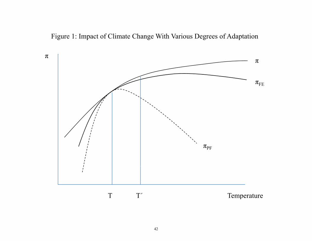
Figure 1: Impact of Climate Change With Various Degrees of Adaptation

ππ

πFE

πPF

T T´ TemperatureT T Temperature

42

Figure 2.A: Districts Included in SMD98 Study

Notes: This map shows the 271 districts included in the Sanghi, Mendelsohn and Dinar 1998 study. The states included are: H P j b d U P d h (N h) G j R j hHaryana, Punjab and Uttar Pradesh (North); Gujarat, Rajasthan (Northwest); Bihar, Orissa, West Bengal (East); Andhra Pradesh, Karnakata, Madhya Pradesh, Maharastra, Tamil Nadu (South). The major agricultural state excluded is Kerala.

43

Figure 2.B: Districts Included in Regressions

Notes: This map shows the 218 districts with output data for all years 1960-1999. The bulk of the lost districts (relative to the y (SMD98 dataset) are from the East, especially Bihar and West Bengal.

44

Figure 3:

05

1015

20da

ys

0 5 10 15 20 25 30 35 40 45bin

Notes: Each one­degree C bin is indicated by the upper limit, e.g. 20 indicates a day with mean temperaturein (19,20]. Growing season is June­September (122 days).

1960­1999Mean Growing­Season Days in Each Temperature Bin

45

Figure 4:

­15

­10

­50

510

Mea

n di

ffere

nce 

in n

umbe

r of d

ays

20 25 30 35 40Daily mean temperature

Notes: Each one­degree C bin is indicated by the upper l imit, e.g. 30 corresponds to mean temperature (29,30].All  temperatures below 22C and above 38C are grouped. Growing season is June­September (122 days).Years: 1960­1999; Sample: districts wi th output data for all years.

Scenario: +.5 deg C mean temperature increaseChange in Distribution of Temperatures

46

Figure 5:

­4­2

02

4N

umbe

r of d

ays

0 5 10 15 20 25 30 35 40 45 50Bin

Notes: Each one­degree C bin is indicated by its upper limit, e.g. 30 corresponds to mean temperature (29,30].Source: Hadley A1F1 model, rescaled. Growing season is June­September (120 days).

National; 1990s to 2010­2039Change in Distribution of Growing Season Daily Mean Temperatures

47

Figure 6:

­10

­50

5N

umbe

r of d

ays

0 5 10 15 20 25 30 35 40 45 50Bin

Notes: Each one­degree C bin is indicated by its upper limit, e.g. 30 corresponds to mean temperature (29,30].Source: Hadley A1F1 model, rescaled. Growing season is June­September (120 days).

National; 1990s to 2070­2099Change in Distribution of Growing Season Daily Mean Temperatures

48

Figure 7:

01

23

45

6M

ean 

sum

 of a

bsol

ute 

resid

uals

20 25 30 35 40Bin

Notes: Each one­degree C bin is indicated by the upper limit, e.g. 30 corresponds to mean temperature (29,30].All temperatures below 22C and above 38C are grouped. Growing season is June­September (122 days).Years: 1960­1999; Sample: districts with output data for all years.

Regression: District Fixed Effects and Cubic Year TrendResidual Variation in Mean Temperatures

49

Figure 8:

­.4­.2

0.2

.4

22 23 24 25 26 27 28 29 30 31 32 33 34 35 36 37 38 39

Point Estimate +/­ 2 Standard Deviations

Notes: P lots coefficients from FGLS regression of yield on number of growing season days in each bin, plus districtfixed effects, monthly precipitation (and squares) and regional cubic time trends. Each 1­degree C bin is indicated by itsupper limit, e.g. 24 indicates a day in with mean temperatures in (23,24] C. The (29,30] bin is the omittedcategory, so estimates are relative to the effect of a day in (29,30]. Temperatures below 22 C and above 38Care grouped. Sample: 218 districts with output data for all years 1960­1999.

Estimated Impact of Temperature Bins on Yield

50

Figure 9.A:

­.3­.2

­.10

.1

22 23 24 25 26 27 28 29 30 31 32 33 34 35 36 37 38 39

Point Estimate +/­ 2 Standard Deviations

Notes: Plots coefficients from FGLS regression of y ield on number of growing season days in each bin, plus districtfixed effects, monthly  precipitation (and squares) and regional cubic time trends. Each 1­degree C bin is indicated by  itsupper limit, e.g. 24 indicates a day in with mean temperatures in (23,24] C. The (29,30] bin is the omittedcategory , so estimates are relative to the effect of a day  in (29,30]. Temperatures below 22 C and above 38Care grouped. Sample: 218 districts with output data for all years 1960­1999.

1960­1979Estimated Impact of Temperature Bins on Yield

Figure 9.B:

­1­.5

0.5

1

22 23 24 25 26 27 28 29 30 31 32 33 34 35 36 37 38 39

Point Estimate +/­ 2 Standard Deviations

Notes: Plots coefficients from FGLS regression of y ield on number of growing season days in each bin, plus districtfixed effects, monthly  precipitation (and squares) and regional cubic time trends. Each 1­degree C bin is indicated by  itsupper limit, e.g. 24 indicates a day in with mean temperatures in (23,24] C. The (29,30] bin is the omittedcategory , so estimates are relative to the effect of a day  in (29,30]. Temperatures below 22 C and above 38Care grouped. Sample: 218 districts with output data for all years 1960­1999.

1980­1999Estimated Impact of Temperature Bins on Yield

51

Mean: 2,479.1; N:8720Regressors RMSE Number Share Number Share Number Share Number Share Number ShareConstant only 204.38 6826 0.783 5069 0.581 3304 0.379 1730 0.198 994 0.114District FEs 53.72 2168 0.249 235 0.027 40 0.005 2 0.000 0 0.000District FEs, Linear Year 52.58 2058 0.236 206 0.024 33 0.004 0 0.000 0 0.000District FEs, Quadratic Year 52.15 2031 0.233 212 0.024 36 0.004 1 0.000 0 0.000District FEs, Cubic Year 52.10 2025 0.232 208 0.024 33 0.004 0 0.000 0 0.000District and Year FEs 35.52 753 0.086 18 0.002 0 0.000 0 0.000 0 0.000District and Year*Region FEs 28.51 374 0.043 3 0.000 0 0.000 0 0.000 0 0.000District and Year*State FEs 21.29 104 0.012 2 0.000 0 0.000 0 0.000 0 0.000

Mean: 2,489.3; N:8720Regressors RMSE Number Share Number Share Number Share Number Share Number ShareConstant only 211.53 6855 0.786 5146 0.590 3489 0.400 1984 0.228 1093 0.125District FEs 56.43 2379 0.273 295 0.034 47 0.005 3 0.000 0 0.000District FEs, Linear Year 55.28 2287 0.262 247 0.028 41 0.005 2 0.000 0 0.000District FEs, Quadratic Year 54.83 2271 0.260 245 0.028 44 0.005 3 0.000 0 0.000District FEs, Cubic Year 54.76 2264 0.260 244 0.028 42 0.005 2 0.000 0 0.000District and Year FEs 37.00 853 0.098 22 0.003 0 0.000 0 0.000 0 0.000District and Year*Region FEs 29.62 418 0.048 5 0.001 0 0.000 0 0.000 0 0.000District and Year*State FEs 22.03 130 0.015 2 0.000 0 0.000 0 0.000 0 0.000

Mean: 2,495.9; N:8720Regressors RMSE Number Share Number Share Number Share Number Share Number ShareConstant only 216.36 6876 0.789 5193 0.596 3602 0.413 2144 0.246 1165 0.134District FEs 58.51 2517 0.289 325 0.037 55 0.006 5 0.001 0 0.000District FEs, Linear Year 57.33 2419 0.277 282 0.032 48 0.006 3 0.000 0 0.000District FEs, Quadratic Year 56.88 2424 0.278 278 0.032 52 0.006 5 0.001 0 0.000District FEs, Cubic Year 56.78 2427 0.278 270 0.031 47 0.005 3 0.000 0 0.000District and Year FEs 38.24 948 0.109 30 0.003 1 0.000 0 0.000 0 0.000District and Year*Region FEs 30.55 477 0.055 8 0.001 0 0.000 0 0.000 0 0.000District and Year*State FEs 22.71 143 0.016 3 0.000 0 0.000 0 0.000 0 0.000

Mean: 2,499.5; N:8720Regressors RMSE Number Share Number Share Number Share Number Share Number ShareConstant only 219.12 6881 0.789 5224 0.599 3660 0.420 2246 0.258 1233 0.141District FEs 59.91 2601 0.298 356 0.041 64 0.007 7 0.001 0 0.000District FEs, Linear Year 58.72 2521 0.289 318 0.036 50 0.006 6 0.001 0 0.000District FEs, Quadratic Year 58.24 2517 0.289 300 0.034 53 0.006 5 0.001 0 0.000District FEs, Cubic Year 58.13 2519 0.289 300 0.034 48 0.006 5 0.001 0 0.000District and Year FEs 39.13 1011 0.116 32 0.004 1 0.000 0 0.000 0 0.000District and Year*Region FEs 31.23 519 0.060 9 0.001 0 0.000 0 0.000 0 0.000District and Year*State FEs 23.24 170 0.019 3 0.000 0 0.000 0 0.000 0 0.000

Panel 4: Degree-Day Upper Bound of 36 C

District*year observations differing from predicted value by more than300 deg-days (C)

Notes: Table counts residuals from regressions of district*year observations on regressors listed in row headings. Cell entries are number ofresiduals of absolute value greater than or equal to the cutoffs given in the column headings.Years: 1960-1999; Sample: 218 districts withoutput data for all years.

60 deg-days (C) 120 deg-days (C) 180 deg-days (C) 240 deg-days (C)

District*year observations differing from predicted value by more than60 deg-days (C) 120 deg-days (C)

Panel 3: Degree-Day Upper Bound of 35 C

180 deg-days (C) 240 deg-days (C) 300 deg-days (C)

Panel 2: Degree-Day Upper Bound of 34 C

District*year observations differing from predicted value by more than60 deg-days (C) 120 deg-days (C) 180 deg-days (C) 240 deg-days (C) 300 deg-days (C)

Appendix Table 2.A: Residual Variation in Growing Season Degree-Days with Alternative Upper Bounds

District*year observations differing from predicted value by more than60 deg-days (C) 120 deg-days (C)

Panel 1: Degree-Day Upper Bound of 33 C

180 deg-days (C) 240 deg-days (C) 300 deg-days (C)

52