The Impact of Broadband on U.S. Agriculture: An Evaluation of the

The Impact of Broadband on U.S. Agriculture: An

Evaluation of the USDA Broadband Loan Program

Amy M. G. Kandilov Ivan T. Kandilov Xiangping Liu Mitch Renkow

RTI North Carolina North Carolina North Carolina

International State University State University State University [email protected] [email protected] [email protected] [email protected]

Selected paper Prepared for Presentation at the Agricultural and Applied Economics Association’s

2011 AAEA &NAREA Joint Annual Meeting Pittsburgh, Pennsylvania, July 24-26, 2011

Copyright 2011 by Amy M.G. Kandilov, Ivan T. Kandilov, Xiangping Liu, and Mitch Renkow.

All rights reserved. Readers may make verbatim copies of this document for non-commercial

purposes by any means, provided that this copyright notice appears on all such copies.

1

1. Introduction

Increasing the availability of broadband in rural communities has been an important U.S. rural

development policy goal over the past decade.1 Since 2000, federal broadband loan programs

authorized under consecutive Farm Bills have directed more than $1.8 billion to private

telecommunications providers in 40 states with the explicit goal of making high-speed data

transmission capacity available to rural residents and businesses. Most recently, the American

Recovery and Reinvestment Act of 2009 authorized $2.5 billion in new federal funding for these

same purposes (Kruger 2009).

Arguments in favor of these programs are supported by research projecting large economic

benefits from widespread broadband deployment (Crandall and Jackson 2001; Crandall et al.

2007). However, these projections obscure the fact that the distribution of these benefits is not

likely to be uniform, either spatially or across industries. For example, a recent study comparing

economic outcomes in communities that did or did not receive broadband loans found evidence

that the loan program created a range of impacts – some positive, some negative – that varied

across industries and across county types (Kandilov and Renkow 2010).

One particularly interesting finding in the Kandilov and Renkow (2010) study is that

agriculture is one of the industries that experienced positive outcomes (in terms of payroll and

number of establishments) in counties receiving broadband loans vis-à-vis non-recipient

counties. In this paper, we further explore the impact of broadband loans on the agricultural

industry. We employ a variety of program evaluation econometric techniques to ascertain

whether or not various indicators of economic performance in the agricultural sector –

commodity sales, production expenses, farm income, and farm size – have been positively

affected by the broadband loan program. The analysis is conducted using county-level data from

2

the U.S. Census of Agriculture (Ag. Census), the county being the smallest level of geographic

disaggregation for which we have data on both the receipt of broadband loans and performance

indicators for agriculture.2

1.1 Why Should Acess to High-speed Internet Matter for Farmers?

There are several reasons why the availability of (high-speed) internet might boost farm

profitability. The internet can substantially reduce the costs of interaction between spatially

dispersed market participants and provide real-time access to information relevant for both

production and marketing decisions of farmers (see Just and Just 2001). It can greatly facilitate

access to current weather and pricing information for inputs and output; it can also speed

technology adoption and improve management practices. All of these improvements can result

in a reduction in farmers’ costs and an increase in their revenue, ultimately leading to higher

profits.

In particular, consider the farmer’s profit maximization problem, equation (1) below:

(1) LPQPLPTCQPTR LQLQ

LQ ),(),(max

, ,

where is farm profit; Q and L are the quantities of output produced and inputs purchased,

respectively; QP and LP are the market prices of output and inputs, and fixed costs are

suppressed for simplicity. Access to (high-speed) internet can increase total revenue (TR) in two

ways. First, it allows farmers to search for new customers for their output, which may lead to an

increase in output produced, Q . Second, farmers might be able to find buyers willing to pay a

higher price than what they currently receive, which leads to a higher output price, QP . On the

other hand, having access to high-speed internet may reveal less costly sources inputs such as

3

seeds, fertilizers, and farm equipment, thereby lowering the price of inputs farmers face, LP .

Finally, access to (high-speed) internet can increase the diffusion of better management practices

that can help farmers produce the same amount of output with fewer inputs.3 All of these factors

can lead to higher revenue or lower costs or both, resulting in higher profits for farmers with

access to (high-speed) internet.

1.2 Empirical Findings

To our knowledge, we are the first to systematically evaluate the impact of increased

access to high-speed internet (via the USDA low-cost broadband loan programs) on the U.S.

agricultural sector nationwide. To estimate the impact of receiving a broadband loan and hence

increased access to high-speed internet on farm sales, costs, and other economic outcomes, we

employ a panel difference-in-differences (DID) fixed effects model as well as a DID propensity

score matching method. We use nationwide county-level data from the Ag. Census in 1997,

2002, and 2007, coupled with data on broadband loan receipt from the USDA. The pilot

broadband loan program was a nationwide program that was introduced in 2000; while the

current broadband loan program started after the 2002 Farm Bill took effect. The goal of the two

programs has been to supply low-cost broadband loans to small U.S. communities.

Our results are consistent with expectations. First, we show that the USDA broadband

loans have a positive effect on high-speed internet use among U.S. farmers – we find that

counties which have received a loan have a higher number of farms that use high-speed internet.

Then, we demonstrate that access to high-speed internet via the USDA broadband loans boosts

farm revenue by about 6 percent. In particular, our baseline estimates suggest that in counties

which received either a pilot broadband loan, administered before 2003, or a current broadband

4

loan, administered following the Farm Bill of 2002, total commodity sales increased by 6.6 and

6.1 percent, respectively, after the loan receipt. Further, the results suggest that total farm

expenditure rose about 3.2 (3.4) percent in counties which received a pilot (current) broadband

loan. Given that we find an increase in farm expenditure following the receipt of the broadband

loans, these estimates imply that farm output in counties receiving the broadband loans must

have increased as a result of increased access to high-speed internet. Overall, our estimates

imply that farm profits have risen about 3 percent as a result of the broadband loans.

Further, we provide evidence that the increase in total commodity sales in counties that

received either of the broadband loans is primarily driven by an increase in crop sales. Sales of

livestock and animal products appear less sensitive to broadband internet access. The current

broadband loan program does not seem to affect total farm acreage, but the earlier pilot loan

program appears to have increased acreage by about 3.6 percent, possibly due to lags in acreage

adjustment. Also, both types of broadband loans are associated with an increase in the number

of farms with positive crop sales in the recipient county. The number of farms with positive

livestock and animal products sales is unaffected by either of the broadband loans.

1.3 Related Literature

There is a large empirical literature on farmers’ computer use that generally focuses on the farm

and farmer characteristics that lead to computer adoption. Examples include Huffman and

Mercier (1991); Hoag et al. (1999); as well as Smith et al. (2004), the last two of which analyze a

sample of Great Plains farmers. Also, Putler and Zilberman (1988) study computer adoption

patterns of farmers in Tulare County, California; and Batte et al. (1990) examine a sample of

Ohio commercial farmers, while Amponsah (1995) studies commercial farmers in North

5

Carolina. Most of these studies provide evidence that the farmer’s age and education and the

size of the farm operation affect computer adoption. Another related strand of the literature

analyzes farmer and farm characteristics affecting both internet adoption and use. Examples

include Smith et al. (2004); Mishra and Park (2005); and Briggeman and Whitacre (2010).

These studies also indicate that farm operator’s age and education play a role in the internet

adoption decision and the intensity of use.

While there is substantial literature on farmers’ computer and internet adoption and use,

there is little previous research on the impact of internet access on agricultural performance.

When it comes to high-speed internet, to our knowledge, there is no previous work done at all,

likely because broadband has only become more readily available in the last 10 to 15 years. The

only relevant work that we were able to locate is an Agricultural and Resource Economics

Newsletter from the Giannini Foundation of Agricultural Economics at the University of

California-Davis by Smith and Paul (2005). Using self-reported survey data obtained from

farmers from the Great Plains in 2000, Smith and Paul (2005) compute that 27 percent of the

Great Plains farmers reported financial gains of about $3,800 (farmers’ estimates of returns)

from using the internet and 42 percent of farmers reported cost savings of an average of 14

percent. The farmers in the survey reported the most beneficial feature of the internet was

finding information on input pricing or agricultural commodity markets. These estimates of the

financial benefits of access to the internet, however, may be difficult to generalize to farmers in

other regions (for example, as Smith and Paul (2005) note, internet marketing may not be as

much of an option for Midwestern grain and livestock farmers as for operators in other parts of

the country). Also, using more objective economic measures, instead of farmers’ estimated

6

financial returns and benefits, may be more appropriate when evaluating the overall economic

impact of the internet on the U.S. agricultural sector.

Finally, our work is also related to the nascent empirical literature analyzing the impact

of broadband on economic performance at the macro level or at the industry level. No work in

this literature has studied the agricultural sector specifically, although as was mentioned earlier

Kandilov and Renkow (2010) found evidence that the USDA broadband loan programs have had

a positive effect on the agricultural sector’s payroll and number of establishments. Other work

in this literature includes Stenberg et al. (2009) who use county-level data to provide evidence

that rural counties with greater broadband access also had greater economic growth. Gillett et al.

(2006) use data on broadband availability between 1998 and 2002 and find that high-speed

internet had a significant positive impact on local employment and the number of businesses

establishments, especially in IT-intensive sectors, but not on wages.4 Shideler et al. (2007)

employ county-level broadband availability data in Kentucky and also uncover a positive impact

of broadband on employment growth in certain sectors. The last two studies indicate that the

positive effects of high-speed internet are smaller in rural counties. In contrast, we present

evidence below that for the agricultural sector, the impacts of high-speed internet are uniformly

positive across urban and rural counties; that is, we find no evidence that a rural-urban divide

exists when it comes to the impacts of broadband on U.S. agriculture.

The rest of the paper is organized as follows. The next section provides details on the

USDA broadband loan programs. Section 3 describes our data and presents summary statistics.

Section 4 outlines the econometric model that we use to identify the impact of increased access

to high-speed internet on farm sales, expenditure, and farm acreage. We discuss our results in

section 5, which also presents a number of robustness checks. Section 6 concludes.

7

2. USDA Broadband Loan Program

In December 2000, Congress authorized a pilot broadband loan program to help expand

broadband access in underserved rural communities. Program eligibility criteria included having

a population of 20,000 or less, having no prior access to broadband, and providing a minimum

matching contribution of 15 percent by recipients of the loan. Loans were extended mainly to

small telecommunications services firms at varying (subsidized) interest rates; most participating

communities qualified for a “hardship rate” of 4 percent (Cowan 2008).

Administered by the USDA’s Rural Utilities Service (RUS), loans worth $180 million

were made in 2002 and 2003 to broadband providers serving 98 communities located in 13

states. Beginning with the 2002 Farm Bill, funding for the current (post-pilot) broadband loan

program was expanded. Program operations were modified due to problems with repayment:

more than one-quarter of the loans extended via the pilot broadband loan program were defaulted

(USDA 2007). As a result, RUS imposed tighter equity and loan security requirements. Another

concern with both the pilot and current programs relates to an overly broad definition of what

constitutes a “rural” community. For example, a 2005 audit by the USDA’s Inspector General

chided RUS for having extended nearly 12 percent of total loan funding to suburban

communities located near large cities (USDA, Office of Inspector General 2005). A follow-up

audit found that this situation was not remedied, noting that between 2005 and 2008 broadband

loans were extended to 148 communities within 30 miles of cities with populations greater than

200,000 – including Chicago and Las Vegas (USDA, Office of Inspector General 2009).

3. Data

Information on which counties obtained loans under the pilot broadband loan program and the

8

current broadband loan program was obtained from the USDA’s Rural Development broadband

program website for all the counties in the U.S.5 As previously discussed, the pilot broadband

loan program was introduced in 2000, while the current broadband loan program started after the

2002 Farm Bill took effect. Therefore, no counties had received any loans by 1997, and by

2002, only the pilot loans had been administered. By 2007, loans from the current broadband

loan program were administered as well. For each county, we construct four treatment variables

that show if a given county has received at least one of either the pilot or the current broadband

loans. The first two variables, Pilot_BBLPct and BBLPct are indicator variables equal to one in

year t and afterwards if county c has at least one community which has received a pilot or a

current broadband loan in year t, respectively.6 The other two variables, N_ Pilot_BBLPct and

N_BBLPct, show the exact number of communities in county c that have received a pilot or a

current broadband loan, respectively.

To estimate the impact of a broadband loan receipt, and hence increased access to high-

speed internet, on farming activities, we use county-level data from the Ag. Census. The county

is the smallest level of geographic disaggregation for which we have information on receipt of

the broadband loans as well as performance indicators for farms. While, with some exceptions,

the USDA does provide data on the actual communities that received broadband loans,

nationwide, comprehensive agricultural performance data is only available at the county level.

Data on farm sales, expenditure, other income, crops and livestock sales, farm acreage and the

number of farms with positive sales were all taken from the Ag. Censuses of 1997, 2002, and

2007. For a number of our robustness checks, we also used data on county population and

income per capita from the U.S. Census of Population.

9

Table 1 presents summary statistics for two sets of counties in the U.S. – those who

received at least one broadband loan, and those who did not. As of 2007, approximately 14

percent of all counties contained at least one community which had received a USDA broadband

loan.

Panel A of Table 1 provides means and standard deviations for a set of key outcome

variables for 1997, the last Ag. Census year prior to the authorization of the pilot broadband loan

program, as well as for 2007, the most recent Ag. Census for which we have data on whether or

not a county had received a broadband loan. Counties that have received broadband loans tend

to be smaller in population. This is unsurprising, given the stated intent of the program is to

target smaller, rural communities. Interestingly, though, there are no significant differences in

mean income per capita between recipient and non-recipient counties. Likewise, there is little

difference between the two types of counties in terms of the other indicators of agricultural

performance, with the exception of livestock sales, which are somewhat higher in non-recipient

counties.

Panel B of Table 1 indicates that many counties contained more than one community

receiving a broadband loan. On average, 2.6 communities received broadband loans in each

county for which any loan was received. Likewise, 3.8 pilot broadband loans were received per

recipient county. Thus, broadband loans tended to be spatially clustered to some extent.

4. Econometric Strategy

To identify the impacts of the USDA’s promotional broadband loan programs (i.e. the effect of

access to high-speed internet) on farm sales, expenditure, other farm-related income, farm

10

acreage, as well as crop and animal sales, we specify the following reduced-form panel DID

fixed effects model:

(2) ctctctcttcct BBLPBBLPPilotln 321 _)( βX ,

where )( ctln is the natural logarithm of the respective dependent variable in county c and in

Ag. Census year t, t = 1997, 2002, 2007. The county fixed effects, c , capture county-specific

characteristics that are time-invariant. The year dummies, t , capture economy-wide shocks that

affect all farms. The coefficients of interest are 1 and 2 – the coefficients measuring the

impact of the two broadband loan programs, the pilot ( ctBBLPPilot _ ) and the current program

( ctBBLP ). In our baseline specification, ctBBLPPilot _ and ctBBLP are indicator variables equal

to one if a county c has received at least one pilot broadband loan ( ctBBLPPilot _ = 1) or at least

one loan from the current broadband loan program ( ctBBLP = 1) by year t. In alternative

specification, we also use the number of pilot ( ctBBLPPilotN __ ) or the number of current

broadband loans ( ctBBLPN _ ) that a county has received by year t. We also show that the

estimates of the impact of the broadband loans are robust to inclusion of time-varying county-

specific covariates, such as county population and income per capita, that may affect the

dependent variable and may potentially be correlated with broadband loan receipt. These

variables are included in the matrix ctX . Finally, ct , is a classical error term.

Another robustness check we perform employs a propensity score matching (PSM)

method. This method was developed by Heckman, Ichimura, and Todd (1997), extending the

original work of Rosenbaum and Rubin (1983) for cross-sectional data. Because we have panel

data, we use the DID version of the PSM method developed by Heckman, Ichimura, Smith, and

11

Todd (1998) specifically for panel data setting. Different from the PSM method for cross-

sectional data, the DID version accommodates for selection on time-invariant (county-level)

unobservables.7

To evaluate the impact of the USDA broadband loans, this method matches (and then

compares) counties that received a broadband loan with counties that did not receive a loan

based on their observable characteristics before any of the counties received a loan (pre-

treatment characteristics).8 We use what is known as the radius matching protocol with a

bandwidth of 0.001 to carry out the DID version of PSM method in our context. Specifically, we

implement this method in two stages. In the first stage, we estimate the probability of broadband

loan receipt using a set of pre-treatment conditional variables and a logistic regression. We

include all variables that affect both the incidence of the broadband loans and the outcomes of

interest, such as farm sales and total expenditure, as conditional variables in the logistic

regression. In the second stage, we compare the outcome variables between the two groups of

counties – the group that received the broadband loans and a group of appropriately matched

counties that did not. The second group consists of counties whose predicted probabilities from

the first stage logistic regressions (propensity scores) fall within 0.001 (radius) of the propensity

scores of the counties that received broadband loans. We then calculate the impact of the

broadband loans on those counties which received them (i.e. the average treatment effect on the

treated) by taking the difference in the differences (post-broadband loan program minus pre-

broadband loan program) of the outcomes between the group of counties that received broadband

loans and the matched group that did not.9 The Appendix provides further details on the

matching procedure.

12

Finally, to investigate the impact of access to high-speed internet (i.e. the effect of the

low-cost USDA broadband loans) on the number of farms with positive sales and other income,

as well as the number of farms with positive crop and animal sales, instead of the linear DID

fixed effects model (2), we use a fixed-effects Poisson model for count data (see, e.g., Cameron

and Trivedi, 1998, pp. 280-282).

5. Results

5.1 The Impact of the USDA Broadband Loans on High-speed Internet Use among U.S.

Farmers

We start by providing direct evidence of the impact of the USDA broadband loan programs on

internet use – in particular, high-speed internet use – among U.S. farmers. Farm-related

information on access to (high-speed) internet was not collected in the 1997 Ag. Census, as this

was prior to the initiation of the pilot broadband loan program (and there was little, if any,

broadband available in rural communities). In the 2002 and 2007 Ag. Censuses, information was

collected on the number of farms with an internet connection. Only in 2007 was specific

information on the number of farms with high-speed internet connection recorded. We take

advantage of this limited data on access to high-speed internet in 2007 to show that counties that

have received a loan through the pilot or the current broadband loan programs by 2007 do in fact

have a higher number of farms with access to high-speed internet vis-a-vis non-recipient

counties. This provides evidence that the broadband loans succeeded in increasing the

penetration and use of broadband in recipient counties.

Panels A and B of Table 2 present the results of cross-sectional Poisson count models

estimated using data from 2007. The dependent variable is the number of farms with access to

high-speed internet. In Panel A, we employ the indicator variable for broadband loan receipt as

13

the treatment variable, whereas in Panel B, we use the actual number of loans received. We

further check the robustness of the results by estimating a baseline model with all counties

(columns 1, 3, 4, and 6), and only counties with a population smaller then 20,000 (columns 2 and

5).

The estimates in Table 2 supports the hypothesis that counties which received at least one

of either the pilot or the current broadband loan also have a larger number of farms with access

to both internet in general and high-speed internet in particular More specifically, the estimates

in column 4 of Panel A indicate that 11.7 percent, or 28 more farms, at the mean (of 239 farms

with high-speed internet access), had access to high-speed internet in counties that received at

least one of the current broadband loans, while 32.8 percent more farms had access to high-speed

internet in counties that received a pilot broadband loan. The latter impact declines to 17.9

percent when county population and income per capita are included in the Poisson regression.

Similar positive and statistically significant estimates are obtained when the number of

broadband loans received, instead of the incidence of the loans, is used as the treatment variable

in Panel B of Table 2. Overall, the results provide a strong indication of a positive effect of the

USDA broadband loans on high-speed internet use among U.S. farmers.

5.2 The Impact of the USDA Broadband Loans on Farm Sales, Expenditure, and Profits:

Baseline Results

In this section, we continue by estimating equation (2) which relates an outcome of interest, for

example farm sales, to receipt of the USDA broadband loans. The first specification we present

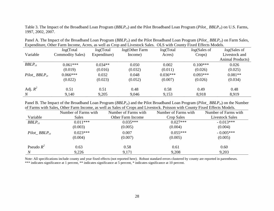
in Panel A of Table 3 contains no covariates and uses total commodity sales as a dependent

variable. The estimates imply that farms in counties which received at least one current USDA

broadband loan experienced about 6.1 percent increase in total commodity sales following the

14

receipt of the loan.10

This impact is both economically and statistically significant. Also, the

results suggest that counties that received at least one of the pilot broadband loans experienced a

6.6 percent increase in total commodity sales. This impact is also economically and statistically

significant, and it is of similar magnitude to that of the current broadband loan program. This is

not surprising since the two broadband loan programs are quite similar, although some of the

differences, as we already outlined earlier, would lead us to expect the pilot program to have a

somewhat larger effect than the current program.

While we have documented an increase in total commodity sales as a result of increased

(high-speed) internet penetration, it is difficult to assess if this is due to higher prices that farmers

can obtain (from higher information efficiency brought about by access to high-speed internet) or

due to increased output (from a larger customer base that they can now locate). Because there is

no information available on average prices that farmers obtain or production quantities (and the

latter would be meaningless if multiple commodities are produced), we next consider farmers’

total expenditures before and after increased availability of high-speed internet. To produce the

same quantity after they gain increased access to (high-speed) internet, farmers would at most

face the same level of expenditure and likely experience lower production costs. Hence, if farm

expenditures rise following the receipt of broadband loans in the county of operation, it must be

the case that inputs and therefore production quantity have increased.

The second column in Panel A of Table 3 reveals that farms’ total expenditure in counties

that have received at least one of the current broadband loans also increased by about 3.4

percent. The impact is statistically significant, but economically, it is only about half the size of

the impact of the current broadband loans on the total commodity sales. This increase in

expenditures signals an increase in production quantity. Overall, farms profits increased by about

15

2.7 percent (= 6.1 - 3.4) as a result of increased access to (high-speed) internet.

The third column in Panel A of Table 3 shows that other farm income (i.e. income from

farm-related sources, such as agricultural services, cash rent and share payments, sales of forest

products, recreational services, patronage dividends, and refunds from cooperatives) has also

increased by about 5 percent in counties that received at least one of either the current or the pilot

broadband loans. Note, however, that while economically significant, these effects are not

estimated precisely enough to be statistically significant.

The fourth column of Panel A of Table 3 presents the impact of the broadband loans on

farm acreage in counties that received at least one of the broadband loans. The estimates reveal

that farm acreage did not change as a result of the current broadband loans, but it rose by about

3.6 percent in counties that received at least one of the pilot broadband loans.11

Similar results

obtain using harvested cropland acreage instead of overall farm acreage as a dependent variable.

Finally, in the last two columns of Panel A, we assess if the growth in commodity sales

due to the increased access to high-speed internet is a result of increased sales of crops or animal

products. The estimates reveal that the positive impact of the broadband loans is larger for crops

than it is for animal products. For both the current and for the pilot broadband loan programs,

the effects are larger in magnitude for crops, although for the pilot loans the two effects are not

significantly different from each other. For the current loans, the impact on crop sales is

estimated to be 10 percent – quite a bit larger than the impact on animal products, which is

estimated to be only 2.6 percent (and not statistically significant).

In Panel B of Table 3, we investigate if receipt of the broadband loans has had any impact

on the number of farms with positive sales and other farm income. The results from the Poisson

county fixed effects model demonstrate that indeed the number of farms with positive sales and

16

other farm income have increased as a result of the better access to high-speed internet brought

about by the broadband loans. For example, the estimated impact of BBLPct, the current

broadband loan program, implies that in counties which received at least one of the current loans,

the number of farms with positive sales has increased by about 7 farms.12

The last two columns

of Panel B show that the number of farms with positive crop sales increased more than the

overall number of farms with positive total sales, while the number of farms with positive animal

sales declined following improved access to high-speed internet. This is may indicate increased

consolidation of animal farms following the increased access to distribution channels and

consumer markets.

5.3 Robustness Checks

Next, we present a number of robustness checks that confirm our initial findings from the

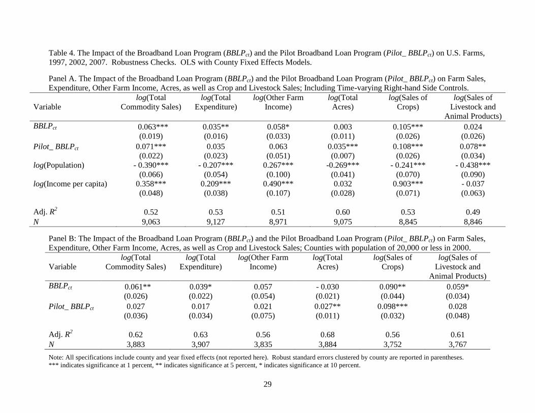
baseline specification (2). We begin in Panel A of Table 4 by adding two county-level time-

varying covariates to our baseline specification – (the natural logarithm of) the county’s

population and (the natural logarithm of) the county’s income per capita – both of which may be

correlated with broadband loan receipt and also may affect farm-related outcomes. Excluding

these variables from the model could lead to biased estimates of the impact of increased

broadband access on farm outcomes. Panel A of Table 4 reports the estimates of the expanded

model that includes the two additional covariates. None of the coefficients differ significantly,

either economically or statistically, from their counterparts in Table 3. Most of the estimated

effects are slightly larger when the two covariates are introduced in Panel A of Table 4. To

conserve space, we only report the results for sales, expenditure, other income, acres, sales of

crops and animal products (Panel A of Table 4). The expanded model estimates for the number

17

of farms with positive sales, other income, as well as crop and animal sales are quite similar to

their counterparts in Panel B of Table 3.13

For the second of our robustness checks, we estimate our baseline specification (2) using

only “small” counties, i.e. counties with population of less than 20,000 people. Note that a

community qualified for a broadband loan if its population was less than 20,000. However, a

community is a smaller geographic unit than a county – for example, there are counties with

more than one community of less than 20,000 people with a broadband loan, resulting in a

number of counties with multiple broadband loans.14

Here, we limit our attention to counties

that resemble “small” communities, i.e. counties that themselves have a population of less than

20,000 people. The results are presented in Panel B of Table 4. The estimates of the impact of

broadband access on county-level farm sales and profits are similar to those obtained with the

full sample of all counties. The only difference is the smaller estimate of the impact of the pilot

broadband loan on both farm sales and expenditure – the estimated impact of the pilot loan on

farm profits is still positive at 1.0 percent.

Our third robustness check involves estimating a DID propensity score matching method.

As before, this method employs DID methodology to estimate the effect of broadband

penetration on farm-related outcomes, but here we compare counties that received at least one

broadband loan (treated) to a carefully selected group of similar counties that did not receive a

loan. The selection rule, as we described earlier, is based on county characteristics prior to the

broadband loan programs. The estimates from the propensity score matching procedure are

presented in Panel C of Table 4. The impacts on farm revenue and expenditure are a little

smaller than the baseline estimates in Panel A of Table 3, but the differences are not statistically

significant. The implied increase in profits for farms with increased access to broadband internet

18

is about 2 percent and 3 percent for the current and the pilot loan programs, respectively, which

is consistent with the baseline estimates in Table 3. Another difference between the PSM results

and the baseline estimates is that the impact of broadband penetration on crop sales is smaller

than what the baseline results indicated. In the case of the current loan program, the PSM

estimator suggests that the impacts of the loans on crop sales is positive and is of roughly the

same size as the impact on animal product sales; in contrast, the baseline estimates reported in

Table 3 indicate that the positive impact of the current broadband loans is more than three times

larger for crop sales than for animal product sales.

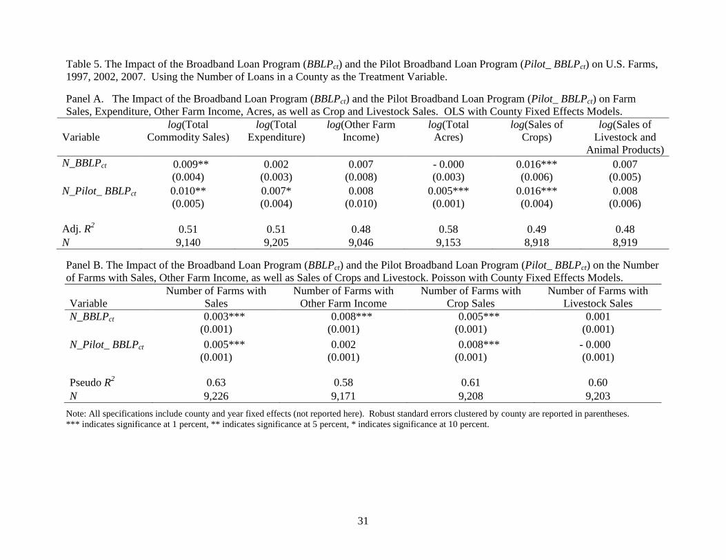
5.4 Alternative Measure for Increased Broadband Access

As previously discussed, counties could receive more than one broadband loan if multiple

communities within the county received a loan. In our fourth robustness check, we incorporate

this information into our specification by using the number of broadband loans received in each

county (current, N_BBLPct, and pilot, N_Pilot_ BBLPct) instead of the broadband loan receipt

indicators (current, BBLPct, and pilot, Pilot_ BBLPct) that we employed earlier. These results are

presented in Panels A and B of Table 5. The estimates are consistent with our previous findings

and indicate that counties that received a larger number of broadband loans, and in which

farmers have better and faster internet access, experienced an increase in commodity sales,

especially crop sales, and a positive but not statistically significant increase in total expenditure.

The results also imply that the average farm profit in counties which received a larger

number of broadband loans increased more than the average farm profit in counties with a

smaller number of loans. Given that the average number of loans in counties that received at

least one loan is 2.612, the estimates imply that the average farm sales in a county that received

19

at least one broadband loan increased by about 2.4 percent (2.4=0.9*2.612). On the other hand,

average farm expenditures in a county that received at least one loan grew by about 0.5 percent,

implying that the average profit in a county that received a broadband loan rose about 2 percent.

Overall, all of the robustness checks indicate that increased access to a broadband internet

connection leads to higher farm sales, expenditures, and profits. Farm sales are estimated to

have risen between 4 and 6 percent due to receipt of a loan from the current broadband loan

program. On the other hand, the impact of a current broadband loan on farm expenditures is

estimated to be between 2.5 and 4 percent, implying that increased access to high-speed internet

has led to an increase in farm profits of about 2 to 3 percent. Similarly, sales increased between

3 and 7 percent, on average, following the receipt of a broadband loan from the pilot program,

and expenditure increased between 2 and 6 percent, leading to an increase in profits between 1

and 3 percent. Most of the evidence suggests that the increase in crop sales, estimated to be

between 5 and 10 percent, is higher than the estimated increase in animal product sales,

estimated to be between 2.5 and 6 percent. Additionally, the results show that other farm income

rose between 2.5 and 6 percent following receipt of a broadband loan from the current program.

Finally, there is no evidence that total farm acres are affected by broadband loans from the

current program, but they do show a slight increase of about 2 to 3 percent as a result of a loan

from the pilot program.

5.5 Difference in Impact of the USDA Broadband Loans by the Farm’s Proximity to an Urban

Continuum

Previous research has found a positive relationship between the economic impacts of broadband

and proximity to densely populated urban areas (see, for example, Gillett et al. 2006; Shideler et

al. 2007; Mack and Grubesic 2009; Kandilov and Renkow 2010). This may be a result of

20

economies of density in broadband supply and/or agglomeration economies affecting broadband

demand. To check whether a similar spatial gradient of the impacts on farm-related outcomes

exists in the case of the broadband loan program, we re-estimated our baseline specification (2)

separately for three different sub-samples of counties – metro counties, rural counties adjacent to

metro counties, and rural counties that are not adjacent to metro counties. We use the USDA’s

Rural-Urban Continuum codes to delineate these groupings.15

These results are displayed in Panels A, B, and C of Table 6. The impact of increased

access to broadband internet on farm sales and costs is quite similar across the three different

types of counties. Except in the case of the pilot broadband loan for Metro counties, the positive

impact of both the current and the pilot loan on farm profits varies between 2 and 3 percent,

which is consistent with the baseline results in Table 3. The estimated positive effect of high-

speed internet availability through the pilot broadband loans in Metro counties is about 6.5

percent (0.065 = 0.073 - 0.008), which is nearly twice as high as the baseline estimate of 3.4

percent (3.4 = 6.6 - 3.2) in Table 3. The impacts of the current and the pilot broadband loans on

other farm-related outcomes (other farm income, farm acreage, as well as crop and animal

(product) sales) are quite similar across the rural-urban continuum. This evidence suggests that

proximity to an urban center does not make a difference when it comes to the positive economic

impacts of high-speed internet on farm sales and profits -- i.e., that the positive economic

impacts of the current and the pilot broadband loan program on U.S. farms found in our baseline

results persists across the rural-urban continuum. This contrasts with the findings of Kandilov

and Renkow (2010) that the positive impacts of broadband loans on (overall) economic activity

are confined to communities located in close proximity to metropolitan centers.

21

6. Conclusion

In this paper we provide an empirical estimate of the impact of the USDA broadband

internet loan programs on U.S. agriculture. High-speed internet can reduce the costs of

interaction between (remote) market participants and provide real-time access to information

relevant for both production and marketing decisions. It can speed access to current weather and

pricing information for inputs and outputs, and it can facilitate technology adoption as well as

management practices. All of these improvements can reduce farmers’ production costs and

raise revenue, ultimately leading to higher profits.

In our empirical analysis, we use nationwide county-level data from the Ag. Census in

1997, 2002, and 2007, coupled with data on broadband loan receipt from the USDA. We

estimate separately the effects of each of the two low-cost broadband loan programs – the pilot

and the current loan program. The pilot broadband loan program is a nationwide program that

was introduced in 2000; while the current broadband loan program started after the 2002 Farm

Bill took effect. The goal of the two programs was to supply low-cost broadband loans to small

U.S. communities.

First, we show that USDA broadband loan receipt is positively associated with high-

speed internet use among U.S. farmers. Then, we employ a variety of program evaluation

econometric techniques, including a panel DID fixed effects model as well as a DID propensity

score matching method, to show that farm sales and expenses, as well as other farm income rose

in counties that received a broadband loan. The estimates indicate that increased access to high-

speed internet leads to about 6 percent growth in farm revenue and about 3 percent growth in

production expenditure, which results in about 3 percent growth in farm profits. Given the

documented increase in farm expenditure following the receipt of the broadband loans, the

22

estimates would imply that farm output in counties receiving the broadband loans must have

increased as a result of increased access to high-speed internet.

We further show evidence that the increase in total commodity sales in counties that

received either one of the broadband loans is primarily driven by an increase in crop sales, and

not sales of livestock and animal products, which appear to be less affected by access to

broadband internet. The current USDA broadband loan program does not seem to affect total

farm acreage, but the earlier pilot loan program appears to have increased farm acreage by about

3.6 percent. Also, receipt of either type of the broadband loans is associated with an increase in

the number of farms with positive total sales and positive crop sales in the recipient county.

23

References

Amponsah, W.A. 1995. “Computer Adoption and Use of Information Services by North Carolina

Commercial Farmers.” Journal of Agriculture and Applied Economics 27(2): 1-7.

Batte, M., E. Jones, and G. Schnitkey. 1990. “Computer Use by Ohio Commercial Farmers.”

American Journal of Agricultural Economics 72(4): 935-945.

Briggeman, B. and B. Whitacre. 2010. “Farming and the Internet: Reasons for Non-use.”

Agricultural and Resource Economics Review 39(3): 571-584.

Cameron, C. and P. Trivedi. 1998. Regression Analysis of Count Data, Econometric Society

Monograph No.30, Cambridge, UK: Cambridge University Press.

Cowan, T. 2008. “An Overview of USDA Rural Development Programs.” CRS Report for

Congress No. RL 31837. Washington, DC: Congressional Research Service.

Crandall, R. and C. Jackson. 2001. “The $500 Billion Opportunity: The Potential Economic

Benefit of Widespread Diffusion of Broadband Internet Access,.” (mimeo), Washington,

DC: Criterion Economics.

Crandall, R., Lehr, W., and R. Litan. 2007. “The Effects of Broadband Deployment on Output

and Employment: A Cross-sectional Analysis of U.S. Data.” Issues in Economic Policy

No. 6. Washington, DC: The Brookings Institution.

Forman, C., Goldfarb, A., and S. Greenstein. 2009. “The Internet and Local Wages:

Convergence or Divergence?” NBER Working Paper No. 14750. Cambridge, MA.

Gillett, S., W. Lehr, C. Osorio, and M. Sirbu. 2006. “Measuring Broadband’s Economic Impact:

Final Report.” National Technical Assistance, Training, Research, and Evaluation Project

#00-07-13829. Washington, DC: U.S. Department of Commerce.

24

Halvorsen , R. and R. Palmquist. 1980. “The Interpretation of Dummy Variables in

Semilogarithmic Equations.” American Economic Review 70: 474-475.

Heckman, J., H. Ichimura, J. Smith, and P. Todd. 1998. “Characterizing Selection Bias Using

Experimental Data.” Econometrica 66(5): 1017-1098.

Heckman, J., H. Ichimura, and P. Todd. 1997. “Matching as an Econometric Evaluation

Estimator: Evidence from Evaluating a Job Training Programme.” Review of Economic

Studies 64(4): 605-654.

Hoag, D., J. Ascough, C. Frasier, and W. Marshall. 1999. “Farm Computer Adoption in the

Great Plains.” Journal of Agricultural and Applied Economics 31(1): 57-67.

Huffman, W. and S. Mercier. 1991. “Joint Adoption of Microcomputer Technologies: An

Analysis of Farmers' Decisions.” Review of Economics and Statistics 73(3): 541-546.

Just D. and R. Just. 2001. “Harnessing the Internet for Farmers - Statistical Data Included.”

Choices 16(2), Spring 2001.

Kandilov, I. and M. Renkow. 2010. “Infrastructure Investment and Rural Economic

Development: An Evaluation of the USDA’s Broadband Loan Program.” Growth and

Change 41(2): 165-191.

Kruger, L. 2009. “Broadband Loan and Grant Programs in the USDA’s Rural Utilities Service.”

Washington, DC: Congressional Research Service.

Mack, E. and T. Grubesic. 2009. Broadband Provision and Firm Location in Ohio: An

Exploratory Spatial Analysis, Tijdschrift voor Economische en Sociale Geografie 100(3):

289-315.

Mishra, A. and T. Park. 2005. “An Empirical Analysis of Internet Use by U.S. Farmers.”

Agricultural and Resource Economics Review 34(2): 253-264.

25

Putler, D. and D. Zilberman. 1988. “Computer Use in Agriculture: Evidence from Tulare

County, California.” American Journal of Agricultural Economics 70(4): 790-802.

Rosenbaum, P. and D. Rubin. 1983. “The Central Role of the Propensity Score in

Observational Studies for Causal Effects.” Biometrika 70: 41-55.

Shideler, D., N. Badasyan, and L. Taylor. 2007. “The Economic Impact of Broadband

Deployment in Kentucky.” Federal Reserve Bank of St. Louis Regional Economic

Development 3(2): 88-118.

Smith, A., R. Goe, M. Kemey, and C.M. Paul. 2004. “Computer and Internet Use by Great Plains

Farmers.” Journal of Agricultural and Resource Economics 29(3): 481-500.

Smith, A. and C.M. Paul. 2005. “Does the Internet Increase Farm Profits?” Giannini Foundation

of Agricultural Economics, U.C. - Davis, ARE Update, Vol. 9, No. 2, Nov./Dec.

Stenberg, P., M. Morehart, S. Vogel, J. Cromartie, V. Breneman, and D. Brown. 2009.

“Broadband Internet’s Value for Rural America” Economic Research Report No. ERR-

78. Washington, DC: USDA

USDA. 2007. “USDA Rural Development: Bringing Broadband to Rural America.” Washington,

DC: USDA. Available at http://www.usda.gov/oig/webdocs/09601-04-TE.pdf.

USDA, Office of Inspector General, Southwest Region. 2005. “Audit Report: Rural Utilities

Service Broadband Grant and Loan Programs.” Audit Report 09601-4-TE. Available at

www.usda.gov/oig/webdocs/090641-04-TE.pdf.

USDA, Office of Inspector General, Southwest Region. 2009. “Audit Report: Rural Utilities

Service Broadband Grant and Loan Programs.” Audit Report 09601-8-TE. Available at

www.usda.gov/oig/webdocs/090641-08-TE.pdf.

26

Tables

Table 1. Summary Statistics

Panel A: Summary Statistics for Outcome Variables and Covariates

Pre-Broadband Loans, 1997 Post-Broadband Loans, 2007

Counties with Either Loan Counties with No Loan Counties with Either Loan Counties with No Loan

Variable Mean St. Dev. Mean St. Dev. Mean St. Dev. Mean St. Dev.

Total Commodity Sales 80,741 91,935 85,415 163,599 97,495 119,117 98,322 189,951

Total Production Expenditure 63,103 69,986 66,785 124,339 79,340 96,588 78,520 148,884

Other Farm Income 1,595 1,299 1,502 2,059 4,037 4,008 3,388 4,509

Total Farm Acres 303 261 310 408 294 247 299 393

Crop Sales 41,501 57,270 42,877 113,153 48,954 67,994 47,403 116,370

Livestock and Animal Products Sales 39,526 61,611 43,279 84,195 49,344 85,131 51,724 109,449

Population 59,866 188,385 91,176 295,044 69,490 242,439 100,506 320,284

Income per Capita 26,669 5,369 26,176 6,033 29,525 6,170 30,350 8,227

No Obs. 373 2,699 373 2,699

Note: All figures are in 1,000’s 2007 U.S. dollars, except those for acres (in 1,000 acres), population, and income per capita.

Panel B: Summary Statistics for Broadband Loan Treatment Variables

Pre-Broadband Loans, 1997 Post-Pilot Broadband Loan, 2002 Post-Broadband Loans, 2007

Variable Mean St. Dev. Mean St. Dev. Mean St. Dev.

Broadband Loan

Receipt 0 0 0 0

0.095

(289 counties) 0.293

Number of Broadband Loans

(for counties with at least one loan) 0 0 0 0

2.612

(755 loans) 2.509

Pilot Broadband Loan

Receipt 0 0

0.032

(98 counties) 0.177

0.032

(98 counties) 0.177

Number of Pilot Broadband Loans

(for counties with at least one pilot loan) 0 0

3.847

(377 loans) 3.124

3.847

(377 loans) 3.124

No Obs. 3,072 3,072 3,072

27

Table 2. The Impact of the Broadband Loan Program (BBLPct) and the Pilot Broadband Loan Program (Pilot_ BBLPct) on High-

speed Internet Use among U.S. Farmers, 2007. Poisson County Fixed Effects Models.

Panel A. Using an Indicator for a Broadband Loan Receipt in a County as the Treatment Variable.

Variable Number of Farms with Internet Number of Farms with High-speed Internet

BBLPct 0.165***

(0.040)

0.236***

(0.063)

0.140***

(0.037)

0.111***

(0.043)

0.163***

(0.056)

0.010**

(0.039)

Pilot_ BBLPct 0.215***

(0.043)

0.224***

(0.064)

0.132***

(0.043)

0.284***

(0.043)

0.357***

(0.057)

0.165***

(0.045)

log(Population)

- -

0.295***

(0.012) - -

0.298***

(0.013)

log(Income per capita)

- -

- 0.565***

(0.078) - -

- 0.382***

(0.082)

Pseudo R2 0.25 0.35 0.46 0.25 0.38 0.46

N 3,174 1,348 3,148 3,170 1,346 3,144

Panel B. Using the Number of Loans in a County as the Treatment Variable.

Variable Number of Farms with Internet Number of Farms with High-speed Internet

N_BBLPct 0.042***

(0.008)

0.069***

(0.025)

0.035***

(0.008)

0.039***

(0.009)

0.052**

(0.021)

0.032***

(0.009)

N_Pilot_ BBLPct 0.032***

(0.007)

0.047***

(0.011)

0.007

(0.010)

0.047***

(0.007)

0.081***

(0.009)

0.012

(0.011)

log(Population)

- -

0.295***

(0.013) - -

0.298***

(0.013)

log(Income per capita)

- -

- 0.556***

(0.078) - -

- 0.372***

(0.081)

Pseudo R2 0.25 0.34 0.45 0.25 0.38 0.45

N 3,174 1,348 3,148 3,170 1,346 3,144 Note: Robust standard errors clustered by county are reported in parentheses. *** indicates significance at 1 percent, ** indicates significance at 5 percent,

* indicates significance at 10 percent.

28

Table 3. The Impact of the Broadband Loan Program (BBLPct) and the Pilot Broadband Loan Program (Pilot_ BBLPct) on U.S. Farms,

1997, 2002, 2007.

Panel A. The Impact of the Broadband Loan Program (BBLPct) and the Pilot Broadband Loan Program (Pilot_ BBLPct) on Farm Sales,

Expenditure, Other Farm Income, Acres, as well as Crop and Livestock Sales. OLS with County Fixed Effects Models.

Variable

log(Total

Commodity Sales)

log(Total

Expenditure)

log(Other Farm

Income)

log(Total

Acres)

log(Sales of

Crops)

log(Sales of

Livestock and

Animal Products)

BBLPct 0.061***

(0.019)

0.034**

(0.016)

0.050

(0.032)

0.002

(0.011)

0.100***

(0.026)

0.026

(0.025)


(0.022)

0.032

(0.023)

0.048

(0.052)

0.036***

(0.007)

0.093***

(0.026)

0.081**

(0.034)

Adj. R2 0.51 0.51 0.48 0.58 0.49 0.48

N 9,140 9,205 9,046 9,153 8,918 8,919

Panel B. The Impact of the Broadband Loan Program (BBLPct) and the Pilot Broadband Loan Program (Pilot_ BBLPct) on the Number

of Farms with Sales, Other Farm Income, as well as Sales of Crops and Livestock. Poisson with County Fixed Effects Models.

Variable

Number of Farms with

Sales


Other Farm Income


Crop Sales


Livestock Sales

BBLPct 0.011***

(0.003)

0.035***

(0.005)

0.027***

(0.004)

- 0.013***

(0.004)


(0.004)

0.007

(0.007)

0.055***

(0.005)

- 0.005***

(0.005)

Pseudo R2 0.63 0.58 0.61 0.60

N 9,226 9,171 9,208 9,203

Note: All specifications include county and year fixed effects (not reported here). Robust standard errors clustered by county are reported in parentheses.

*** indicates significance at 1 percent, ** indicates significance at 5 percent, * indicates significance at 10 percent.

29


1997, 2002, 2007. Robustness Checks. OLS with County Fixed Effects Models.

Panel A. The Impact of the Broadband Loan Program (BBLPct) and the Pilot Broadband Loan Program (Pilot_ BBLPct) on Farm Sales,

Expenditure, Other Farm Income, Acres, as well as Crop and Livestock Sales; Including Time-varying Right-hand Side Controls.

Variable

log(Total

Commodity Sales)

log(Total

Expenditure)

log(Other Farm

Income)

log(Total

Acres)

log(Sales of

Crops)

log(Sales of

Livestock and

Animal Products)

BBLPct 0.063***

(0.019)

0.035**

(0.016)

0.058*

(0.033)

0.003

(0.011)

0.105***

(0.026)

0.024

(0.026)


(0.022)

0.035

(0.023)

0.063

(0.051)

0.035***

(0.007)

0.108***

(0.026)

0.078**

(0.034)

log(Population) - 0.390***

(0.066)

- 0.207***

(0.054)

0.267***

(0.100)

-0.269***

(0.041)

- 0.241***

(0.070)

- 0.438***

(0.090)

log(Income per capita) 0.358***

(0.048)

0.209***

(0.038)

0.490***

(0.107)

0.032

(0.028)

0.903***

(0.071)

- 0.037

(0.063)

Adj. R2 0.52 0.53 0.51 0.60 0.53 0.49

N 9,063 9,127 8,971 9,075 8,845 8,846

Panel B: The Impact of the Broadband Loan Program (BBLPct) and the Pilot Broadband Loan Program (Pilot_ BBLPct) on Farm Sales,

Expenditure, Other Farm Income, Acres, as well as Crop and Livestock Sales; Counties with population of 20,000 or less in 2000.

Variable

log(Total

Commodity Sales)

log(Total

Expenditure)

log(Other Farm

Income)

log(Total

Acres)

log(Sales of

Crops)

log(Sales of

Livestock and

Animal Products)

BBLPct 0.061**

(0.026)

0.039*

(0.022)

0.057

(0.054)

- 0.030

(0.021)

0.090**

(0.044)

0.059*

(0.034)

Pilot_ BBLPct 0.027

(0.036)

0.017

(0.034)

0.021

(0.075)

0.027**

(0.011)

0.098***

(0.032)

0.028

(0.048)

Adj. R2 0.62 0.63 0.56 0.68 0.56 0.61

N 3,883 3,907 3,835 3,884 3,752 3,767



30

Table 4 (Cont’d.). The Impact of the Broadband Loan Program (BBLPct) and the Pilot Broadband Loan Program (Pilot_ BBLPct) on

U.S. Farms, 1997, 2002, 2007. Robustness Checks. OLS with County Fixed Effects Models.

Panel C: The Impact of the Broadband Loan Program (BBLPct) and the Pilot Broadband Loan Program (Pilot_ BBLPct) on Farm Sales,

Expenditure, Other Farm Income, Acres, as well as Crop and Livestock Sales; Propensity Score Matching (Radius) method.

Variable

log(Total

Commodity Sales)

log(Total

Expenditure)

log(Other Farm

Income)

log(Total

Acres)

log(Sales of

Crops)

log(Sales of

Livestock and

Animal Products)

BBLPct 0.043**

(0.022)

0.024

(0.018)

0.097**

(0.041)

- 0.012

(0.009)

0.045

(0.033)

0.041

(0.029)


(0.020)

0.020

(0.023)

0.044

(0.050)

0.021*

(0.011)

- 0.009

(0.025)

0.060*

(0.031)

Note: All specifications in Panel C include county and year fixed effects (not reported here). Robust standard errors clustered by county are reported in

parentheses. See the text and Appendix II for the details on the propensity score matching procedure. There are 71 counties which obtained a pilot broadband

loan and 203 counties which obtained a regular broadband loan used in the matching procedure.


31


1997, 2002, 2007. Using the Number of Loans in a County as the Treatment Variable.

Panel A. The Impact of the Broadband Loan Program (BBLPct) and the Pilot Broadband Loan Program (Pilot_ BBLPct) on Farm

Sales, Expenditure, Other Farm Income, Acres, as well as Crop and Livestock Sales. OLS with County Fixed Effects Models.

Variable

log(Total

Commodity Sales)

log(Total

Expenditure)

log(Other Farm

Income)

log(Total

Acres)

log(Sales of

Crops)

log(Sales of

Livestock and

Animal Products)

N_BBLPct 0.009**

(0.004)

0.002

(0.003)

0.007

(0.008)

- 0.000

(0.003)

0.016***

(0.006)

0.007

(0.005)

N_Pilot_ BBLPct 0.010**

(0.005)

0.007*

(0.004)

0.008

(0.010)

0.005***

(0.001)

0.016***

(0.004)

0.008

(0.006)

Adj. R2 0.51 0.51 0.48 0.58 0.49 0.48

N 9,140 9,205 9,046 9,153 8,918 8,919

Panel B. The Impact of the Broadband Loan Program (BBLPct) and the Pilot Broadband Loan Program (Pilot_ BBLPct) on the Number

of Farms with Sales, Other Farm Income, as well as Sales of Crops and Livestock. Poisson with County Fixed Effects Models.

Variable


Sales


Other Farm Income


Crop Sales


Livestock Sales

N_BBLPct 0.003***

(0.001)

0.008***

(0.001)

0.005***

(0.001)

0.001

(0.001)

N_Pilot_ BBLPct 0.005***

(0.001)

0.002

(0.001)

0.008***

(0.001)

- 0.000

(0.001)

Pseudo R2 0.63 0.58 0.61 0.60

N 9,226 9,171 9,208 9,203



32

Table 6. The Impact of the Broadband Loan Program (BBLPct) and the Pilot Broadband Loan Program (Pilot_ BBLPct) on U.S.

Farms, 1997, 2002, 2007. Estimates by the County Position in the Rural-Urban Hierarchy.

Panel A. Metro Counties.

Variable

log(Total

Commodity Sales)

log(Total

Expenditure)

log(Other Farm

Income)

log(Total

Acres)

log(Sales of

Crops)

log(Sales of

Livestock and

Animal Products)

BBLPct 0.049

(0.036)

0.031

(0.032)

0.025

(0.060)

0.027

(0.022)

0.092**

(0.043)

0.010

(0.056)

Pilot_ BBLPct 0.073**

(0.029)

0.008

(0.041)

0.104

(0.085)

0.050***

(0.013)

0.054

(0.062)

0.104

(0.074)

Adj. R2 0.65 0.65 0.61 0.69 0.64 0.61

N 3,133 3,156 3,097 3,136 3,060 3,051

Panel B. Rural Counties Adjacent to a Metro County.

Variable

log(Total

Commodity Sales)

log(Total

Expenditure)

log(Other Farm

Income)

log(Total

Acres)

log(Sales of

Crops)

log(Sales of

Livestock and

Animal Products)

BBLPct 0.054*

(0.031)

0.034

(0.024)

0.015

(0.051)

0.009

(0.021)

0.086*

(0.045)

0.024

(0.035)

Pilot_ BBLPct 0.056*

(0.034)

0.038

(0.030)

0.150

(0.093)

0.052***

(0.010)

0.157***

(0.034)

0.028

(0.043)

Adj. R2 0.61 0.61 0.55 0.63 0.58 0.64

N 3,120 3,145 3,098 3,126 3,050 3,054

Panel C. Rural Counties Not Adjacent to a Metro County.

Variable

log(Total

Commodity Sales)

log(Total

Expenditure)

log(Other Farm

Income)

log(Total

Acres)

log(Sales of

Crops)

log(Sales of

Livestock and

Animal Products)

BBLPct 0.062*

(0.033)

0.025

(0.026)

0.134**

(0.055)

- 0.035***

(0.010)

0.100**

(0.042)

0.024

(0.043)

Pilot_ BBLPct 0.057

(0.045)

0.036

(0.042)

- 0.067

(0.085)

0.002

(0.012)

0.069*

(0.035)

0.093*

(0.056)

Adj. R2 0.68 0.69 0.62 0.74 0.64 0.66

N 2,885 2,901 2,850 2,888 2,808 2,814 Note: All specifications include county and year fixed effects (not reported here). Robust standard errors clustered by county are reported in parentheses.


33

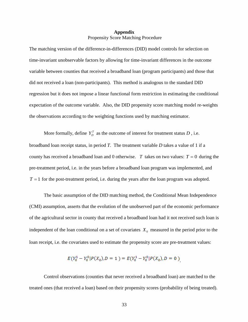
Appendix

Propensity Score Matching Procedure

The matching version of the difference-in-differences (DID) model controls for selection on

time-invariant unobservable factors by allowing for time-invariant differences in the outcome

variable between counties that received a broadband loan (program participants) and those that

did not received a loan (non-participants). This method is analogous to the standard DID

regression but it does not impose a linear functional form restriction in estimating the conditional

expectation of the outcome variable. Also, the DID propensity score matching model re-weights

the observations according to the weighting functions used by matching estimator.

More formally, define T

DY as the outcome of interest for treatment status D , i.e.

broadband loan receipt status, in period T. The treatment variable D takes a value of 1 if a

county has received a broadband loan and 0 otherwise. T takes on two values: 0T during the

pre-treatment period, i.e. in the years before a broadband loan program was implemented, and

1T for the post-treatment period, i.e. during the years after the loan program was adopted.

The basic assumption of the DID matching method, the Conditional Mean Independence

(CMI) assumption, asserts that the evolution of the unobserved part of the economic performance

of the agricultural sector in county that received a broadband loan had it not received such loan is

independent of the loan conditional on a set of covariates 0X measured in the period prior to the

loan receipt, i.e. the covariates used to estimate the propensity score are pre-treatment values:

.

Control observations (counties that never received a broadband loan) are matched to the

treated ones (that received a loan) based on their propensity scores (probability of being treated).

34

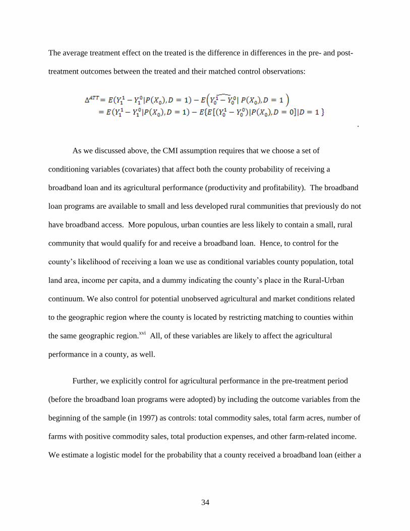
The average treatment effect on the treated is the difference in differences in the pre- and post-

treatment outcomes between the treated and their matched control observations:

.

As we discussed above, the CMI assumption requires that we choose a set of

conditioning variables (covariates) that affect both the county probability of receiving a

broadband loan and its agricultural performance (productivity and profitability). The broadband

loan programs are available to small and less developed rural communities that previously do not

have broadband access. More populous, urban counties are less likely to contain a small, rural

community that would qualify for and receive a broadband loan. Hence, to control for the

county’s likelihood of receiving a loan we use as conditional variables county population, total

land area, income per capita, and a dummy indicating the county’s place in the Rural-Urban

continuum. We also control for potential unobserved agricultural and market conditions related

to the geographic region where the county is located by restricting matching to counties within

the same geographic region.xvi

All, of these variables are likely to affect the agricultural

performance in a county, as well.

Further, we explicitly control for agricultural performance in the pre-treatment period

(before the broadband loan programs were adopted) by including the outcome variables from the

beginning of the sample (in 1997) as controls: total commodity sales, total farm acres, number of

farms with positive commodity sales, total production expenses, and other farm-related income.

We estimate a logistic model for the probability that a county received a broadband loan (either a

35

pilot loan or a current loan). We then construct the propensity score for each county using the

estimated coefficients from the logistic regression.

We construct the counterfactual for each county that received a broadband loan using the

counties that did not receive a loan but have similar estimated propensity scores. We use radius

matching and impose a bandwidth of 0.001. Specifically, we construct the counterfactual for a

county with a broadband loan using all the counties that do not have a loan and have an

estimated propensity score that is within 0.0005 of the propensity score of the treated county.

Also, as we already discussed, in order to control any potential bias due to the difference in

agricultural production patterns across agricultural regions, we restrict the matching to counties

within the same region.

More formally, the constructed counterfactual is

.

where j indexes counties that did not receive a broadband loan and i indexes counties that

received a loan (with county j being matched to county i based on their estimated propensity

scores). The matrix, ),( jiw , contains the weights assigned to the jth control county that is

matched to the ith treated county. The matching estimator constructs an estimate of the expected

unobserved counterfactual for each county that received a broadband loan by taking a weighted

average of the difference in pre-treatment and post-treatment outcomes for each matched county

without a broadband loan.

36

To compute the average impact of broadband loan programs on the agricultural outcomes

(sales, expenditures, other farm income, acres, etc.) for treated counties, i.e. for counties that

received a broadband loan, we use the standard definition of the Average Treatment Effect on the

Treated, or the ATT :

.

In the equation above, N is the number of the counties with a loan,

is the

difference in post-treatment and pre-treatment outcomes in a county i with a broadband loan, and

is the constructed counterfactual for each county i. The average impact of

the broadband loan program is therefore the mean difference in the pre-treatment and post-

treatment differences in the outcomes between the counties with a broadband loan and the

constructed counterfactual outcomes from the matched counties that did not receive such a loan.

After matching, we check if the treated and control counties (those with a broadband loan

and those without one) are balanced on covariates, i.e. if the two groups have similar

characteristics in the pre-broadband loan period, in 1997. If unbalanced, the estimated ATT may

not reflect solely the impact of the broadband loan programs. Instead, it may be a combination

of the impacts of the loan programs and the unbalanced covariates. We rely on t-tests to check if

the means for each covariate are statistically the same between the two groups of counties – the

treated (those with a loan) and the controls (those without a loan). The balancing criteria are

satisfied for all of our covariates, including the dummy variables for agricultural regions as well

as the dummy variables for urban/rural status. This indicates that the two groups of counties –

37

those with a broadband loan and the matched group of counties without a loan – are indeed

observationally equivalent, and it also implies that our estimated ATT reflects solely the impact

of the broadband loan programs.

38

1 Examples of other federally subsidized technological improvements that lower informational

barriers and market transaction costs for the rural population and entrepreneurs include the

establishment of rural delivery routes for the U.S. Postal Service, as well as the construction of

rural roads.

2 USDA provides data on the actual communities that received broadband loans. However,

comprehensive agricultural performance data is only available at the county level.

3 If output rises as a result of higher demand brought about by access to (high-speed) internet, the

amount of inputs will increase, as well.

4 Also, Forman et al.’s (2009) recent working paper reports that the rise in IT has had little

impact on wage growth in rural areas.

5 The USDA’s Rural Development Broadband Program website can be found at the following

address: http://www.usda.gov/rus/telecom/broadband.htm.

6 For the pilot broadband loan program, we assign 2002 as the start year for all counties that

received such a loan. If a county received a loan from the current broadband loan program

before June 1 of a given year, we consider that year as the start year; otherwise, we take the

following year as the start year.

7 The PSM method developed by Rosenbaum and Rubin (1983) accommodates for “selection on

observables”. Any uncontrolled unobservables that affect counties which received the USDA

broadband loan differently from counties that did not would introduce bias in the estimated

effects.

39

8 Note that a natural candidate control (comparison) group is the group of counties in which

potential broadband providers applied for broadband loans but were denied. Unfortunately, the

USDA has retained no information on broadband loan applications that were denied.

9 This DID version of the PSM matching method is analogous to the standard DID fixed effects

regression estimator in (2), but it does not impose a functional form in estimating the conditional

expectation of the outcome variable, and it re-weights the observations according to the

weighting function used by the matching estimator.

10 More precisely, to calculate the percentage change in total commodity sales resulting from a

broadband loan receipt, i.e. increasing BBLPct from 0 to 1, one needs to raise e ( = 2.718) to the

power of the estimated coefficient (0.061 here) and then subtract one (the resulting impact is

0.063 here). This procedure is necessary because of the log-linear specification and the fact that

BBLPct is an indicator variable that only changes discontinuously (see Halvorsen and Palmquist,

1980). However, for small ’s, the differences between and exp( ) -1 is trivial.

11 It is possible that access to broadband internet affects farm acreage with a lag, i.e. the impact

of broadband on acreage takes time to emerge. Hence, the estimates may reflect the fact that the

Pilot broadband loan program started a number of years earlier than the current broadband loan

program.

12 Given the sample average of 710 farms with positive commodity sales per county, a 1.1

percent increase in the number of farms with positive sales in counties that have received at least

one current broadband loan is equivalent to an increase of about 7 farms with positive sales.

13 Another robustness check that we have done extends the baseline specification (2) by

including state-specific time trends which control for state trends potentially correlated with

broadband loan receipt – a complication that may possibly confound the estimation. The results

40

from this expanded specification, which are not reported here to conserve space, are fairly

similar to those from our baseline specification presented in Table 2. One more notable

difference is that the impact on farm expenditure is estimated to be higher than that in Table 2,

which in the case of the current broadband loan implies that the overall impact on farm profits is

positive at 1.2 percent.

14 Also, in a number of instances, broadband loans were given to providers who supplied

broadband access to “small” communities, but the same project also included supplying “large”

(greater than 20,000 people) communities. In this case, while the loans were specifically granted

only for the “small” communities, they were considered to have benefited both the “small” and

the “large” communities.

15 Interested readers can find more details on the USDA Rural-Urban classification at the

following address http://www.ers.usda.gov/briefing/rurality/ruralurbcon. Note that in metro

counties, a large fraction of the workforce commutes to nearby, highly urbanized metro area.

xvi We use 12 regions: Appalachian (NC, VA, KY, TN, WV), Corn Belt and Northern Plains (IL,

IN, OH, IA, MO, KS, NE, ND, SD), California (CA), Delta and Southeast (AR, LA, MS, AL,

GA, SC), Florida (FL), Great Lakes (MI, MN, WI), Mountain I (ID, MT, WY, CO, NV, UT),

Mountain II (AZ, NM), Northeast I (CT, ME, MA, NH, NY, RI, VT), Northeast II (DE, MD, NJ,

PA), Pacific (OR, WA), Southern Plains (OK, TX).

Documents

The Impact of Broadband on U.S. Agriculture: An Evaluation of the