For comments, suggestions or further inquiries please contact:

Philippine Institute for Development StudiesSurian sa mga Pag-aaral Pangkaunlaran ng Pilipinas

The PIDS Discussion Paper Seriesconstitutes studies that are preliminary andsubject to further revisions. They are be-ing circulated in a limited number of cop-ies only for purposes of soliciting com-ments and suggestions for further refine-ments. The studies under the Series areunedited and unreviewed.

The views and opinions expressedare those of the author(s) and do not neces-sarily reflect those of the Institute.

Not for quotation without permissionfrom the author(s) and the Institute.

February 2006

The Research Information Staff, Philippine Institute for Development Studies3rd Floor, NEDA sa Makati Building, 106 Amorsolo Street, Legaspi Village, Makati City, PhilippinesTel Nos: 8924059 and 8935705; Fax No: 8939589; E-mail: publications@pidsnet.pids.gov.ph

Or visit our website at http://www.pids.gov.ph

The Impact of a Philippine-US FTA:The Case of Philippine Agriculture

U-Primo E. Rodriguez and Liborio S. Cabanilla

DISCUSSION PAPER SERIES NO. 2006-06

THE IMPACT OF AN RP-US FTA: THE CASE

OF PHILIPPINE AGRICULTURE

U-Primo E. Rodriguez and Liborio S. Cabanilla

Abstract The paper examines the effect of an RP-US FTA in the Philippine agricultural sector. Using an Applied General Equilibrium (AGE) Model, it analyzes the impact of the removal of tariffs on imports from the US on the various commodities in agriculture and food processing. The simulation results suggest that most of the commodities in these sectors experience gains in output and employment following the removal of Philippine tariffs on its imports from the U.S. It also shows that the benefits of agriculture and food processing from the FTA are larger with a comprehensive removal of tariffs. Keywords: Philippine agriculture production, consumption and employment, foreign and domestic markets, tariff change and removal, economic modelling This paper is part of the “RP-US FTA Research Project” of the Philippine APEC Study Center Network, Philippine Institute for Development Studies. The authors wish to thank Cielito Habito, Mario Lamberte and Erlinda Medalla for their comments on an earlier draft. The usual disclaimer applies.

1

THE IMPACT OF A PHILIPPINES-US FTA: THE CASE OF PHILIPPINE AGRICULTURE

U-Primo E. Rodriguez and Liborio S. Cabanilla

1. INTRODUCTION

This paper analyzes the implications of establishing a free trade area between the

United States (US) and the Philippines. In particular, it evaluates the effects of the

agreement on production, consumption and employment in Philippine agriculture and

food processing.

The analysis is carried out using an Applied General Equilibrium (AGE) model.

This tool has been widely used in the analysis of trade policies in general and regional

trading arrangements in particular.1 Its appeal arises from the explicit treatment

substitution possibilities among various commodities in production and consumption.

Moreover, AGE models capture the interaction between various agents and markets in an

economy. Such models therefore facilitate the analysis of the effects of policies on a wide

range of economic variables.

The remainder of this paper is organized as follows. Section 2 describes the model

that will be used in the analysis. Section 3 discusses the different experiments and key

outcomes. Section 4 concludes.

2. DESCRIPTION OF THE MODEL

The analysis uses a revised version of the AGE model developed by Inocencio et

al. (2001). The original model was designed to evaluate the effects of economic policies,

1 Examples of applications to regional trading agreements are Cororaton (2004), Wolf (2000), Oktaviani and Drynan (2000), Diao and Somwara (2000), Bandara and Yu (2001), Lewis et al. (1999), Lewis et al. (1995).

2

environmental policies and exogenous shocks on different economic variables. To

address the concerns of this paper, the model was revised by disaggregating Philippine

exports and imports by source and destination. In particular, it explicitly identifies

Philippine trade with the US. The succeeding will paragraphs describe the basic features

of the original model. This is followed by an account of the revisions that were made to

suit the objectives of this paper.2

The original model

The original model is disaggregated into 40 goods and services. Eight of these

commodities can be classified as part of Agriculture, Fishery and Forestry. These are (1)

Palay, (2) Corn, (3) Vegetables, fruits and nuts,(4) Coconut and Sugar cane, (5)

Livestock, poultry and other animals, (6) Fishery, (7) Other Agricultural Production, (8)

Forestry. On the other hand, Food processing is composed of (1) Rice and corn milling,

(2) Milled Sugar, (3) Meat manufacturing, (4) Fish Manufacturing, (5) Beverage and

tobacco manufacturing, (6) Other food manufacturing. The remaining 26 commodities of

the model belong to the (other) Industry and Services sectors.

The model has five major blocks. These are production, households, government,

foreign trade and the environment.

Each commodity in the production block has a representative firm that uses

capital, labor and intermediate goods to produce its gross output. This firm is assumed to

be an optimizing agent (i.e., maximizes profits) that is operating in a perfectly

2 The interested reader can consult the appendix for a listing of the equations, variable definitions and disaggregation of the model. For a more comprehensive discussion, also see Inocencio et al (2001).

3

competitive market. The outcomes from the optimization process are used to specify the

input demand and output supply equations in the model.

The output of the representative firm is sold to domestic and foreign markets

(export supply). These are determined by assuming that the firm seeks to maximize its

revenues from selling to these markets. In doing so, the firm is assumed to be constrained

by its gross output, prices and an aggregator represented by a constant elasticity of

transformation (CET) function.

The household block is disaggregated into three income groups. These are low,

middle and high income households. Each of these groups is assumed to have

representative household that is endowed with capital and labor. Payments to capital and

labor, along with net transfer payments, represent the income of these households. This

income is then allocated for savings, taxes and consumption.

The consumption of goods and services is determined through an optimization

process. The representative household is assumed to maximize its utility or satisfaction

by selecting the quantities of goods and services it will consume subject to given prices

and desired spending (income less taxes and savings).

The government generates revenues mainly through taxes on income, transactions

and imports. Its collections are then allocated for goods and services and net transfers.

Any discrepancy between government revenues and outlays is then reflected though the

budget deficit.

4

The foreign trade block captures exports and imports. It is modeled under the

assumption that the Philippines is a price taker in world markets. This assumption

suggests that the import supply and export demand functions are perfectly elastic. Import

demands are determined by imposing the Armington assumption – i.e., imports are

differentiated by source.

The major blocks are integrated by means of equilibrium conditions. The supply

side is composed of the output of domestic firms and imports. On the other hand, the

demand side is composed of government spending on goods and services, household

consumption, intermediate demand and exports (foreign demand). These equilibrium

conditions determine domestic prices in the model.

The data for the model is based primarily on a Social Accounting Matrix (SAM)

that was constructed using the 1994 Input-Output table.

Revisions to the basic model

The basic model does not disaggregate imports and exports by source and

destination. The objectives of the paper therefore make it necessary to modify model in to

explicitly account for Philippine imports coming from and exports going to the US.

The modifications to the model equations were implemented by imposing the

Armington assumption. This suggests that imports from the US are not perfectly

substitutable with those coming from the rest of the world (ROW). Philippine exports to

the US and ROW are also assumed to be differentiated.

5

The import demand equations, by source, are derived as follows. It is assumed

that the objective of the domestic agent is to find the combination of the imports from the

US and ROW that will minimize the total cost of imports. This optimizing process is

implemented under the assumption that total imports and import prices (by source) are

given. It also assumes that the total imports of a specific commodity is a Constant

Elasticity of Substitution (CES) composite of imports from the US and ROW. The first

order conditions from this process are used as the equations for the import demands from

the US and ROW.

The key properties of the resulting equations are as follows. First, the import

demand from a particular source is inversely related to its relative price. In other words,

the Philippine demand for US-made goods will decline if there is an increase in the price

of US imports relative to ROW imports. Second, the import demand from a particular

source is positively related to the demand for total imports. That is, the demand for US

imports (and ROW imports) will rise if the total imports higher.

The specification of the export supply equations, by destination, proceeds along

the same lines. However, the objective of the firm is to find the combination of US and

ROW exports which will maximize the revenues from exporting. The optimizing process

is implemented under the assumption that total exports and export prices (by destination)

are given. It also assumes that the total exports of a given commodity is a Constant

Elasticity of Transformation (CET) composite of exports destined for the US and ROW.

The first order conditions from this process are used as the export supply equations for

the US and ROW.

6

The key properties of the export supply equations are as follows. First, exports to

a particular destination are positively related to its relative price. In other words, domestic

firms want to sell more to the US if there is an increase in US export prices relative to

ROW export prices. Second, exports to a particular destination are positively related to

total exports. That is, US exports (and ROW exports) will rise if total exports higher.

Apart from the revising the equations of the model, there was also a need to

modify the SAM to capture the spatial features of exports and imports. This was

implemented by computing the average share of the US in the Philippine exports and

imports of each commodity. The average shares were calculated using disaggregated

trade data from the Department of Trade and Industry for the period 2001-2003.3 Exports

to and imports from US were then obtained by multiplying the relevant shares to their

respective totals in the SAM.

3. SIMULATION RESULTS

3.1 Description of experiments

In the absence of information regarding the final structure of the free area

between the Philippines and US, six experiments were explored in the simulations.

Experiment A assumes that all Philippine tariffs on US imports are removed. On the

other hand, Experiments B and C focus on the selective removal of Philippine tariffs on

US imports. Experiment B assumes that the tariff removal is confined only to agriculture

and food processing. In contrast, Experiment C exempts these sectors from the tariff

changes.

3 The basic data was downloaded from http://tradeline.dti.gov.ph .

7

For each experiment, there is an additional simulation involving a one percent

increase in a set of export prices. This is an attempt to capture the possible opening-up of

US market to Philippine exports The changes in export prices follows the theme for each

experiment. In Experiment A, the tariff cuts were augmented by an across the board

increase in the export prices of goods destined for the US. On the other hand, only the

export prices of agriculture and food processing were increased for Experiment B.

Finally, only the export prices of goods and services that are not included in agriculture

and food processing were allowed to change in Experiment C.

The model was solved under a Keynesian closure in which the wage rate is

assumed to be exogenously determined.

3.2 Effects on Import Prices

Since the Philippines is assumed to be a small open economy, the elimination

import tariffs will be directly reflected in changes in the domestic price of imports from

the US. As larger tariff cuts lead to larger declines in import prices, the results presented

here therefore reflect the extent to which the country’s domestic markets receive tariff

protection. With tariff rates on imports from the ROW held constant, the elimination of

tariffs on US imports eventually affect the domestic of Philippine imports from all

sources. The magnitude of these changes will now reflect the size of tariff cuts and the

share of the US in total Philippine imports.

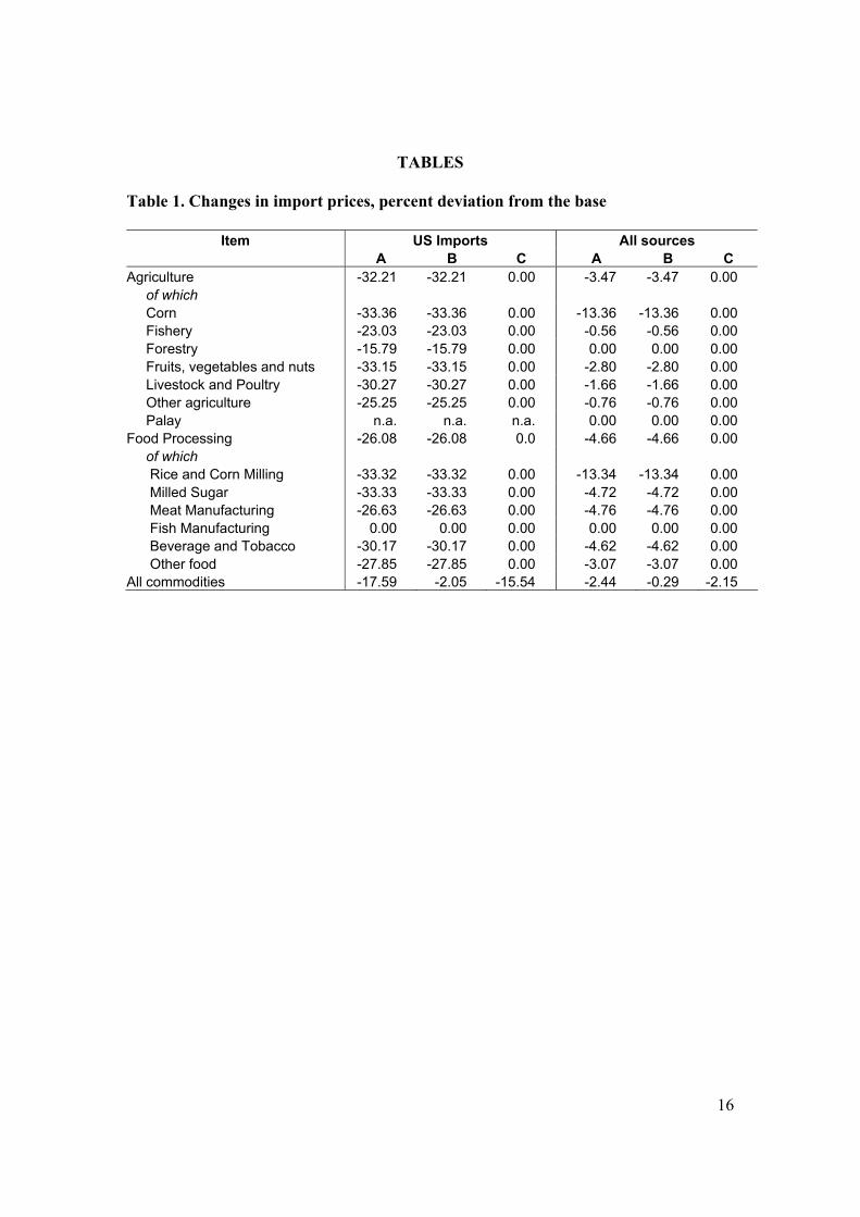
Table 1 shows the changes in the domestic prices of imported goods. Experiments

A and B suggest a 32.21 and 26.08 percent decline in the share weighted average of US

import prices of agriculture and food processing, respectively. In contrast, Experiment C,

8

as it exempts agriculture and food processing, indicates that US import prices remain

constant.

Along with changes in tariff rates for other commodities, these changes translate

to a decline of 2.05 to 17.59 percent in the average import price of all commodities

sourced from the US. These results capture the fact that agriculture and food processing

as a whole receive higher tariff protection than other goods and services. Moreover,

smaller decline in the import prices of all commodities in Experiment B (= -2.05 percent)

compared to in Experiment C (= -15.54 percent) suggests that imports agriculture and

food processing account for a relatively small proportion of total US imports.

3.3 Production and employment

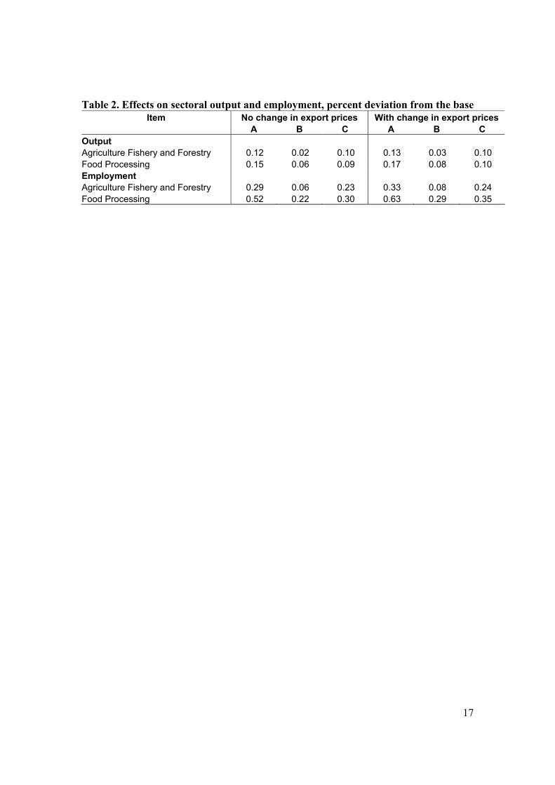
Table 2 shows the potential impacts of an FTA on output and employment. It

indicates that the free trade area is likely to cause an increase in the output of agriculture

(0.02 to 0.13 percent) and food processing (0.06 to 0.17 percent). This also translates into

higher employment. The potential expansion for agriculture is between 0.06 to 0.33

percent. On the other hand, the increase in employment in food processing ranges from

0.22 to 0.52 percent.

The results suggest a number of patterns that are likely to emerge from the

formation of a free trade area with the US. First, the expansion in the output of food

processing is likely to be larger than agriculture. Second, the largest expansion in output

is likely to be realized from a comprehensive elimination of tariffs. This can be seen by

comparing the output responses in Experiment A with the other experiments. Third,

confining the tariff changes to agriculture and food processing generates the least benefits

9

to these sectors. This follows from the finding that Experiment B has the smallest

increases in the output and employment. Fourth, the bulk of the gains to agriculture and

food processing are likely to come from the removal of tariffs elsewhere in the economy.

This can be observed from the finding that the output gains in Experiment C are larger

than in Experiment B. Fifth, the increase in export prices is likely to magnify the

expansion in the aggregate outputs of agriculture and food processing. In Experiment A

for example, the output of food processing is 0.02 percentage points higher in the case

where export prices are allowed to increase.

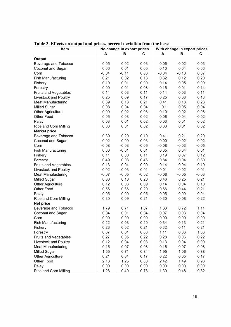
A disaggregated analysis reveals that almost all commodities in agriculture and

food processing are likely to expand with the formation of a free trade area (see Table 3).

Corn is the only commodity that experiences a contraction. Moreover, Meat

Manufacturing and Livestock and Poultry are likely to experience the largest gains in

output. This result generally holds for all experiments. The only exception here is the

relatively large expansion in Fish Manufacturing in Experiment C.

The contraction of Corn output occurs in Experiments A and B. Without going

into the details, this can readily be attributed to the tariff cuts in Corn in particular and

agriculture in general.4 The basis for this statement is the result in Experiment C, which

shows that Corn output expands when it is exempted from the tariff cuts.

The expansion in Meat Manufacturing and Livestock and Poultry may be

explained by the increase in their respective net prices. This implies that producers of

these commodities are receiving more for each unit of the good is sold. The fact that this

4 Without going into the actual data in the model, this can be seen in Table 1 where the cut in the domestic prices of imported corn is among the largest following the tariff cuts.

10

happens despite the decline in the market prices of their output highlights the benefits of

conducting an economywide analysis. The net price of a good is the market price less the

price of intermediate inputs and indirect taxes. With indirect taxes held constant, the

increase in the net price suggests that the prices of intermediate inputs must have declined

by a larger proportion than the market price.

3.4 Results for consumption and household incomes

Table 4 shows that a free trade area with the US can lead to higher incomes for

Philippine households. Moreover, the pattern of changes is similar to what was observed

for outputs. That is, the benefits are largest for Experiments A and C.

Apart from higher incomes, the results for Experiments A and C suggest the

potential for reducing income inequality. This can be seen from the finding that Low

Income (High Income) households experience the largest (smallest) increase incomes. In

contrast, the results for Experiment B indicate that the income increase in the Low

Income household is the smallest among the different groups. This suggests that

confining the removal of trade barriers to agriculture and food processing can actually be

regressive.

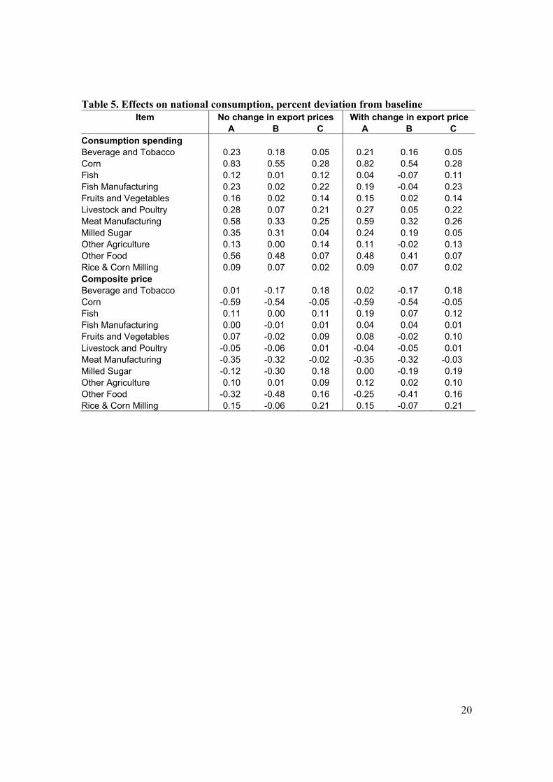
Table 5 shows that the tariff changes lead to higher household consumption of

commodities produced by agriculture and food Processing. In Experiment A, for

example, the changes range from 0.09 percent in Rice and Corn Milling to 0.83 percent in

Corn. As a whole, the increase in consumption is explained mostly by the increase in

household incomes.

11

Differences in the magnitude of the changes across commodities are generally

explained by the composite prices of the commodities.5 In Experiment A, for example,

Rice and Corn Milling experiences the smallest increase in consumption (=0.12 percent)

because it experiences a relatively large increase in its composite price (=0.15 percent).

On the other hand, Corn experiences the largest increase in consumption (=0.83 percent)

because it experiences a relatively large decrease in its composite price (= - 0.59 percent).

Experiments A and B indicate the largest increases in consumption. This reflects the

fact that tariffs on agriculture and food processing were removed in these experiments.

Such a removal of tariff rates lead to relatively large declines (or small increases) in the

composite price of goods. For example, the composite price of Corn declines by 0.59 and

0.54 percent in Experiments A and B, respectively. In contrast, the decline in the

composite price of this commodity is only 0.05 percent in Experiment C.

The results also indicate that the increase in export prices may either raise or reduce

the consumption of goods and services. In Experiment A for example, the removal of

tariffs causes a 0.12 percent increase in the consumption of Fish. However, incorporating

the increase in export prices causes a smaller increase in Fish consumption (0.04

percent). The same pattern is observed for all other commodities except Meat

Manufacturing and Rice and Corn Milling.

3.5 Effects on Trade

As a whole, the free trade area leads to an expansion of trade. Moreover, the

results indicate that the expansion is not limited to trade with the United States.

5 The composite price of a commodity is the weighted average of its domestic and imported component.

12

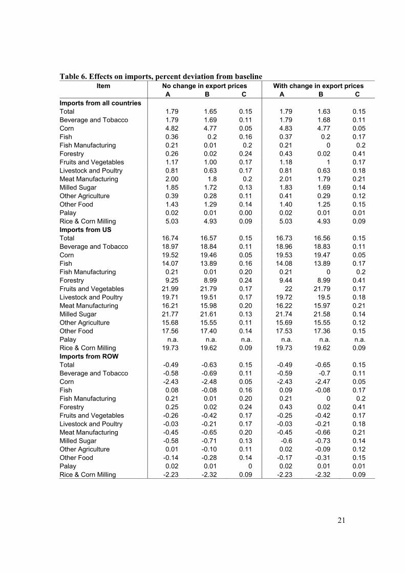
Table 6 indicates the effects of the free trade area on the imports of agriculture

and food processing. It shows that Experiments A and B generate the largest increases in

total imports at 1.79 and 1.65 percent, respectively.6 Despite being exempt from tariff

cuts, total imports of agriculture and food processing also expand in Experiment C.

As expected, the removal of tariffs in Experiments A and B causes an increase in

total imports from the US. This pattern, which is also observed for all commodities in

Table 6, may be explained by two factors. First, the increase in domestic consumption

tends to raise the demand for imports as a whole. Second, the removal of tariffs on US

imports suggest a decline their prices relative to the ROW. Such changes induce a

substitution away from ROW imports towards US imports.

Among the various activities, Corn and Rice and Corn Milling are expected to

have the largest increases in imports (from all sources). This may be explained by the

finding that these commodities are among the activities that experience the largest

increase in imports from the US. Moreover, US imports in these activities account for a

relatively large share of their total imports.7

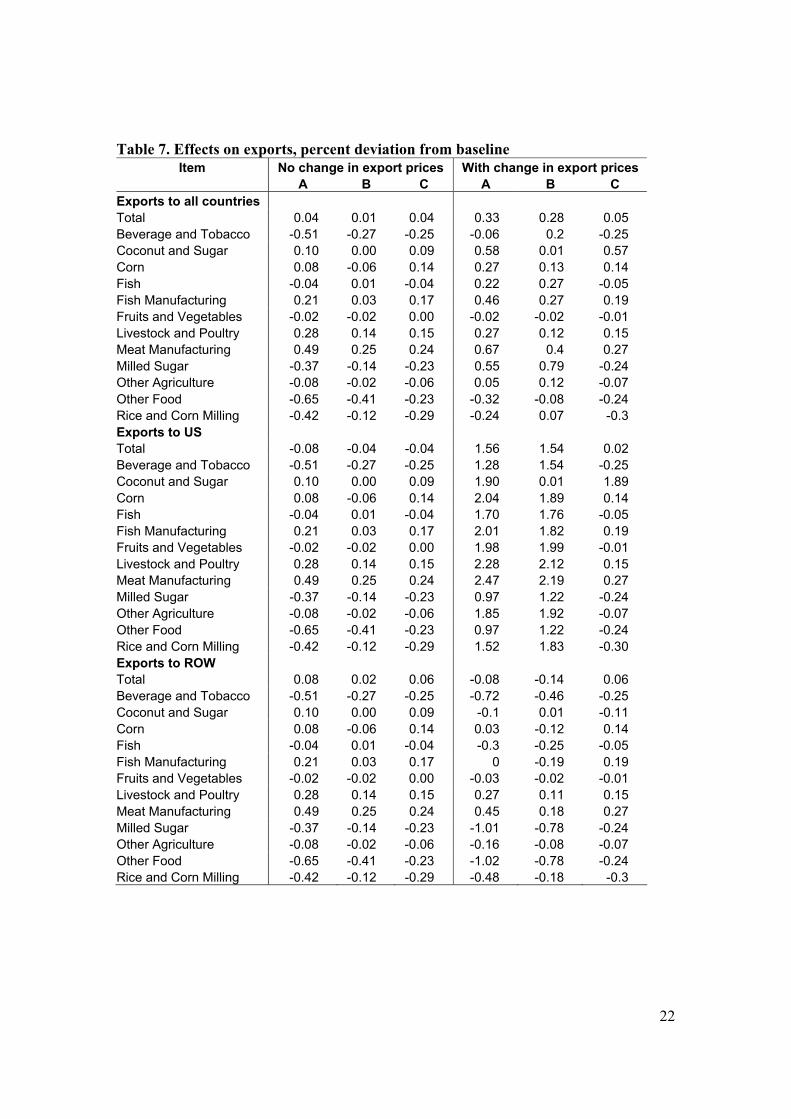
In all cases, the tariff changes lead to a small expansion in the exports of

agriculture and food processing. Table 7 shows that the change in total exports (to all

countries) range from 0.01 to 0.04 percent. These changes are larger when export prices

are also allowed to rise. For example, the increase in total exports (to all countries) in

6 Introducing changes in export prices does not significantly alter this pattern. 7 In the model, approximately 37 percent Corn and Rice and Corn Milling imports are sourced from the US.

13

Experiment A is 0.29 percentage points (=0.33 – 0.04) higher in the presence of higher

export prices.

A disaggregated analysis indicates the mixed responses for exports. Ignoring the

increase in export prices for the moment, Meat Manufacturing, Livestock and Poultry and

Fish Manufacturing consistently experience an expansion in exports. The opposite is true

for Other Agriculture, Milled Sugar, Rice and Corn Milling, Beverage and Tobacco and

Other food.

The expansion in the outputs of all the commodities cited in the previous paragraph

exerts upward pressure on their respective exports. As such, differences in the export

changes can be explained mostly by changes in relative prices. With export prices held

constant, changes in the market price emerge as the key variable in explaining the results.

Meat Manufacturing, for example, had relatively large declines in market prices for all

experiments.8 This implies that the activity experienced the largest increase in the relative

price of exports. In contrast, Other Food had relatively large increases in market prices

for all experiments. This suggests that the relative prices of its exports experienced

relatively large declines.

Introducing changes in export prices generally leads to higher exports of the different

sectors. In Experiment A for example, the most noticeable of these changes are for Fish,

Milled Sugar and Other agriculture. Once again, changes in output and relative prices

help explain these findings. First, in most cases, the increase in export prices also leads to

larger increases in outputs. Ceteris paribus, this stimulates exports. A similar result

8 Recall that the effects on market prices are shown in Table 3.

14

occurs when export prices rise because this makes it more attractive to sell overseas

compared to the domestic market.

4. CONCLUDING REMARKS

The results from the experiments suggest that the formation of a free trade area is

likely to benefit agriculture and food processing. This is reflected in the finding that the

removal of tariff barriers on US imports generally leads to higher output and trade for

these sectors. Moreover, benefits are likely to be larger once effects of changes in export

prices are factored into the analysis.

The simulations also suggest that the coverage of the free trade area has important

implications for agriculture and food processing. Tariff changes confined only to these

sectors do little by way of stimulating output and trade. The gains are likely to be larger

with a comprehensive removal of trade barriers between the US and the Philippines.

15

REFERENCES

Bandara, J. and W. Yu, 2001. How Desirable is the South Asian Free Trade Area? A Quantitative Economic Assessment, SJFI Working Paper No. 16/2001

Cororaton, C., 2004. Philippine-Japan Bilateral Agreements: An Analysis of Possible Effects on Unemployment, Distribution and Poverty in the Philippines Using a CGE-Microsimulation Approach, Discussion Paper No. 2004-1, Philippine Institute for Development Studies, Makati

Diao, X and A. Somwara, 2000. A Dynamic Evaluation of the Effects of a Free Trade Area of the Americas – An Intertemporal., Global General Equilibrium Model, manuscript, International Food Policy Research Institute, Washington D.C.

Inocencio, A., C. Dufournaud and U. Rodriguez, 2001. Impact of Tax Changes on Environmental Emissions: An Applied General Equilibrium Approach for the Philippines, IMAPE Research Paper No. 07, Makati

Lewis, J., S. Robinson and K. Thierfelder, 1999. After the Negotiations: Assessing the Impact of Free Trade Agreements in Southern America, TMD Discussion Paper No. 46, International Food Policy Research Institute, Washington D.C.

Lewis, J., S. Robinson, and Z. Wang, 1995. Beyond the Uruguay Round: Implications of an Asian Free Trade Area, Policy Research Working Paper 1467, World Bank

Oktaviani, R. and R. Drynan, 2000. The Impact of APEC Trade Liberalization on the Indonesian Economy and Agricultural Sector, paper presented at the Third Annual Conference on Global Economic Analysis, Melbourne, June 28-30

Wolf, S, 2000. From Preferences to Reciprocity: General Equilibrium Effects of a Free Trade Area Between the EU and UEMOA, paper presented at the Third Annual Conference on Global Economic Analysis, Melbourne, June 28-30

16

TABLES Table 1. Changes in import prices, percent deviation from the base

Item US Imports All sources A B C A B C

Agriculture -32.21 -32.21 0.00 -3.47 -3.47 0.00 of which Corn -33.36 -33.36 0.00 -13.36 -13.36 0.00 Fishery -23.03 -23.03 0.00 -0.56 -0.56 0.00 Forestry -15.79 -15.79 0.00 0.00 0.00 0.00 Fruits, vegetables and nuts -33.15 -33.15 0.00 -2.80 -2.80 0.00 Livestock and Poultry -30.27 -30.27 0.00 -1.66 -1.66 0.00 Other agriculture -25.25 -25.25 0.00 -0.76 -0.76 0.00 Palay n.a. n.a. n.a. 0.00 0.00 0.00 Food Processing -26.08 -26.08 0.0 -4.66 -4.66 0.00 of which Rice and Corn Milling -33.32 -33.32 0.00 -13.34 -13.34 0.00 Milled Sugar -33.33 -33.33 0.00 -4.72 -4.72 0.00 Meat Manufacturing -26.63 -26.63 0.00 -4.76 -4.76 0.00 Fish Manufacturing 0.00 0.00 0.00 0.00 0.00 0.00 Beverage and Tobacco -30.17 -30.17 0.00 -4.62 -4.62 0.00 Other food -27.85 -27.85 0.00 -3.07 -3.07 0.00 All commodities -17.59 -2.05 -15.54 -2.44 -0.29 -2.15

17

Table 2. Effects on sectoral output and employment, percent deviation from the base Item No change in export prices With change in export prices

A B C A B C Output Agriculture Fishery and Forestry 0.12 0.02 0.10 0.13 0.03 0.10 Food Processing 0.15 0.06 0.09 0.17 0.08 0.10 Employment Agriculture Fishery and Forestry 0.29 0.06 0.23 0.33 0.08 0.24 Food Processing 0.52 0.22 0.30 0.63 0.29 0.35

18

Table 3. Effects on output and prices, percent deviation from the base Item No change in export prices With change in export prices

A B C A B C Output Beverage and Tobacco 0.05 0.02 0.03 0.06 0.02 0.03 Coconut and Sugar 0.06 0.01 0.05 0.10 0.04 0.06 Corn -0.04 -0.11 0.06 -0.04 -0.10 0.07 Fish Manufacturing 0.21 0.02 0.18 0.32 0.12 0.20 Fishery 0.10 0.01 0.09 0.14 0.05 0.09 Forestry 0.09 0.01 0.08 0.15 0.01 0.14 Fruits and Vegetables 0.14 0.03 0.11 0.14 0.03 0.11 Livestock and Poultry 0.25 0.09 0.17 0.25 0.08 0.18 Meat Manufacturing 0.39 0.18 0.21 0.41 0.18 0.23 Milled Sugar 0.08 0.04 0.04 0.1 0.05 0.04 Other Agriculture 0.09 0.02 0.08 0.10 0.02 0.08 Other Food 0.05 0.03 0.02 0.06 0.04 0.02 Palay 0.03 0.01 0.02 0.03 0.01 0.02 Rice and Corn Milling 0.03 0.01 0.02 0.03 0.01 0.02 Market price Beverage and Tobacco 0.39 0.20 0.19 0.41 0.21 0.20 Coconut and Sugar -0.02 0.00 -0.03 0.00 0.02 -0.02 Corn -0.08 -0.03 -0.05 -0.08 -0.03 -0.05 Fish Manufacturing 0.00 -0.01 0.01 0.05 0.04 0.01 Fishery 0.11 0.00 0.11 0.19 0.07 0.12 Forestry 0.49 0.03 0.46 0.84 0.04 0.80 Fruits and Vegetables 0.13 0.04 0.09 0.14 0.04 0.10 Livestock and Poultry -0.02 -0.03 0.01 -0.01 -0.02 0.01 Meat Manufacturing -0.07 -0.05 -0.02 -0.08 -0.05 -0.03 Milled Sugar 0.33 0.13 0.20 0.46 0.25 0.21 Other Agriculture 0.12 0.03 0.09 0.14 0.04 0.10 Other Food 0.56 0.36 0.20 0.66 0.44 0.21 Palay -0.05 0.00 -0.05 -0.05 0.00 -0.04 Rice and Corn Milling 0.30 0.09 0.21 0.30 0.08 0.22 Net price Beverage and Tobacco 1.79 0.71 1.07 1.83 0.72 1.11 Coconut and Sugar 0.04 0.01 0.04 0.07 0.03 0.04 Corn 0.00 0.00 0.00 0.00 0.00 0.00 Fish Manufacturing 0.22 0.03 0.20 0.34 0.13 0.21 Fishery 0.23 0.02 0.21 0.32 0.11 0.21 Forestry 0.67 0.04 0.63 1.11 0.06 1.06 Fruits and Vegetables 0.27 0.05 0.22 0.28 0.06 0.22 Livestock and Poultry 0.12 0.04 0.08 0.13 0.04 0.09 Meat Manufacturing 0.15 0.07 0.08 0.15 0.07 0.08 Milled Sugar 1.55 0.71 0.84 1.95 1.06 0.88 Other Agriculture 0.21 0.04 0.17 0.22 0.05 0.17 Other Food 2.13 1.25 0.88 2.42 1.49 0.93 Palay 0.00 0.00 0.00 0.00 0.00 0.00 Rice and Corn Milling 1.28 0.49 0.78 1.30 0.48 0.82

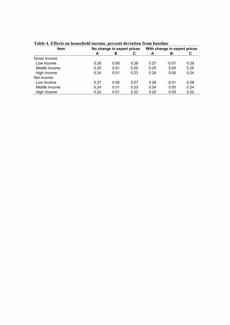
Table 4. Effects on household income, percent deviation from baseline Item No change in export prices With change in export prices

A B C A B C Gross Income Low Income 0.28 0.00 0.28 0.27 -0.01 0.29 Middle Income 0.25 0.01 0.25 0.25 0.00 0.25 High Income 0.24 0.01 0.23 0.24 0.00 0.24 Net Income Low Income 0.27 0.00 0.27 0.26 -0.01 0.28 Middle Income 0.24 0.01 0.23 0.24 0.00 0.24 High Income 0.22 0.01 0.22 0.22 0.00 0.22

20

Table 5. Effects on national consumption, percent deviation from baseline Item No change in export prices With change in export price

A B C A B C Consumption spending Beverage and Tobacco 0.23 0.18 0.05 0.21 0.16 0.05 Corn 0.83 0.55 0.28 0.82 0.54 0.28 Fish 0.12 0.01 0.12 0.04 -0.07 0.11 Fish Manufacturing 0.23 0.02 0.22 0.19 -0.04 0.23 Fruits and Vegetables 0.16 0.02 0.14 0.15 0.02 0.14 Livestock and Poultry 0.28 0.07 0.21 0.27 0.05 0.22 Meat Manufacturing 0.58 0.33 0.25 0.59 0.32 0.26 Milled Sugar 0.35 0.31 0.04 0.24 0.19 0.05 Other Agriculture 0.13 0.00 0.14 0.11 -0.02 0.13 Other Food 0.56 0.48 0.07 0.48 0.41 0.07 Rice & Corn Milling 0.09 0.07 0.02 0.09 0.07 0.02 Composite price Beverage and Tobacco 0.01 -0.17 0.18 0.02 -0.17 0.18 Corn -0.59 -0.54 -0.05 -0.59 -0.54 -0.05 Fish 0.11 0.00 0.11 0.19 0.07 0.12 Fish Manufacturing 0.00 -0.01 0.01 0.04 0.04 0.01 Fruits and Vegetables 0.07 -0.02 0.09 0.08 -0.02 0.10 Livestock and Poultry -0.05 -0.06 0.01 -0.04 -0.05 0.01 Meat Manufacturing -0.35 -0.32 -0.02 -0.35 -0.32 -0.03 Milled Sugar -0.12 -0.30 0.18 0.00 -0.19 0.19 Other Agriculture 0.10 0.01 0.09 0.12 0.02 0.10 Other Food -0.32 -0.48 0.16 -0.25 -0.41 0.16 Rice & Corn Milling 0.15 -0.06 0.21 0.15 -0.07 0.21

21

Table 6. Effects on imports, percent deviation from baseline Item No change in export prices With change in export prices

A B C A B C Imports from all countries Total 1.79 1.65 0.15 1.79 1.63 0.15 Beverage and Tobacco 1.79 1.69 0.11 1.79 1.68 0.11 Corn 4.82 4.77 0.05 4.83 4.77 0.05 Fish 0.36 0.2 0.16 0.37 0.2 0.17 Fish Manufacturing 0.21 0.01 0.2 0.21 0 0.2 Forestry 0.26 0.02 0.24 0.43 0.02 0.41 Fruits and Vegetables 1.17 1.00 0.17 1.18 1 0.17 Livestock and Poultry 0.81 0.63 0.17 0.81 0.63 0.18 Meat Manufacturing 2.00 1.8 0.2 2.01 1.79 0.21 Milled Sugar 1.85 1.72 0.13 1.83 1.69 0.14 Other Agriculture 0.39 0.28 0.11 0.41 0.29 0.12 Other Food 1.43 1.29 0.14 1.40 1.25 0.15 Palay 0.02 0.01 0.00 0.02 0.01 0.01 Rice & Corn Milling 5.03 4.93 0.09 5.03 4.93 0.09 Imports from US Total 16.74 16.57 0.15 16.73 16.56 0.15 Beverage and Tobacco 18.97 18.84 0.11 18.96 18.83 0.11 Corn 19.52 19.46 0.05 19.53 19.47 0.05 Fish 14.07 13.89 0.16 14.08 13.89 0.17 Fish Manufacturing 0.21 0.01 0.20 0.21 0 0.2 Forestry 9.25 8.99 0.24 9.44 8.99 0.41 Fruits and Vegetables 21.99 21.79 0.17 22 21.79 0.17 Livestock and Poultry 19.71 19.51 0.17 19.72 19.5 0.18 Meat Manufacturing 16.21 15.98 0.20 16.22 15.97 0.21 Milled Sugar 21.77 21.61 0.13 21.74 21.58 0.14 Other Agriculture 15.68 15.55 0.11 15.69 15.55 0.12 Other Food 17.56 17.40 0.14 17.53 17.36 0.15 Palay n.a. n.a. n.a. n.a. n.a. n.a. Rice & Corn Milling 19.73 19.62 0.09 19.73 19.62 0.09 Imports from ROW Total -0.49 -0.63 0.15 -0.49 -0.65 0.15 Beverage and Tobacco -0.58 -0.69 0.11 -0.59 -0.7 0.11 Corn -2.43 -2.48 0.05 -2.43 -2.47 0.05 Fish 0.08 -0.08 0.16 0.09 -0.08 0.17 Fish Manufacturing 0.21 0.01 0.20 0.21 0 0.2 Forestry 0.25 0.02 0.24 0.43 0.02 0.41 Fruits and Vegetables -0.26 -0.42 0.17 -0.25 -0.42 0.17 Livestock and Poultry -0.03 -0.21 0.17 -0.03 -0.21 0.18 Meat Manufacturing -0.45 -0.65 0.20 -0.45 -0.66 0.21 Milled Sugar -0.58 -0.71 0.13 -0.6 -0.73 0.14 Other Agriculture 0.01 -0.10 0.11 0.02 -0.09 0.12 Other Food -0.14 -0.28 0.14 -0.17 -0.31 0.15 Palay 0.02 0.01 0 0.02 0.01 0.01 Rice & Corn Milling -2.23 -2.32 0.09 -2.23 -2.32 0.09

22

Table 7. Effects on exports, percent deviation from baseline Item No change in export prices With change in export prices

A B C A B C Exports to all countries Total 0.04 0.01 0.04 0.33 0.28 0.05 Beverage and Tobacco -0.51 -0.27 -0.25 -0.06 0.2 -0.25 Coconut and Sugar 0.10 0.00 0.09 0.58 0.01 0.57 Corn 0.08 -0.06 0.14 0.27 0.13 0.14 Fish -0.04 0.01 -0.04 0.22 0.27 -0.05 Fish Manufacturing 0.21 0.03 0.17 0.46 0.27 0.19 Fruits and Vegetables -0.02 -0.02 0.00 -0.02 -0.02 -0.01 Livestock and Poultry 0.28 0.14 0.15 0.27 0.12 0.15 Meat Manufacturing 0.49 0.25 0.24 0.67 0.4 0.27 Milled Sugar -0.37 -0.14 -0.23 0.55 0.79 -0.24 Other Agriculture -0.08 -0.02 -0.06 0.05 0.12 -0.07 Other Food -0.65 -0.41 -0.23 -0.32 -0.08 -0.24 Rice and Corn Milling -0.42 -0.12 -0.29 -0.24 0.07 -0.3 Exports to US Total -0.08 -0.04 -0.04 1.56 1.54 0.02 Beverage and Tobacco -0.51 -0.27 -0.25 1.28 1.54 -0.25 Coconut and Sugar 0.10 0.00 0.09 1.90 0.01 1.89 Corn 0.08 -0.06 0.14 2.04 1.89 0.14 Fish -0.04 0.01 -0.04 1.70 1.76 -0.05 Fish Manufacturing 0.21 0.03 0.17 2.01 1.82 0.19 Fruits and Vegetables -0.02 -0.02 0.00 1.98 1.99 -0.01 Livestock and Poultry 0.28 0.14 0.15 2.28 2.12 0.15 Meat Manufacturing 0.49 0.25 0.24 2.47 2.19 0.27 Milled Sugar -0.37 -0.14 -0.23 0.97 1.22 -0.24 Other Agriculture -0.08 -0.02 -0.06 1.85 1.92 -0.07 Other Food -0.65 -0.41 -0.23 0.97 1.22 -0.24 Rice and Corn Milling -0.42 -0.12 -0.29 1.52 1.83 -0.30 Exports to ROW Total 0.08 0.02 0.06 -0.08 -0.14 0.06 Beverage and Tobacco -0.51 -0.27 -0.25 -0.72 -0.46 -0.25 Coconut and Sugar 0.10 0.00 0.09 -0.1 0.01 -0.11 Corn 0.08 -0.06 0.14 0.03 -0.12 0.14 Fish -0.04 0.01 -0.04 -0.3 -0.25 -0.05 Fish Manufacturing 0.21 0.03 0.17 0 -0.19 0.19 Fruits and Vegetables -0.02 -0.02 0.00 -0.03 -0.02 -0.01 Livestock and Poultry 0.28 0.14 0.15 0.27 0.11 0.15 Meat Manufacturing 0.49 0.25 0.24 0.45 0.18 0.27 Milled Sugar -0.37 -0.14 -0.23 -1.01 -0.78 -0.24 Other Agriculture -0.08 -0.02 -0.06 -0.16 -0.08 -0.07 Other Food -0.65 -0.41 -0.23 -1.02 -0.78 -0.24 Rice and Corn Milling -0.42 -0.12 -0.29 -0.48 -0.18 -0.3

23

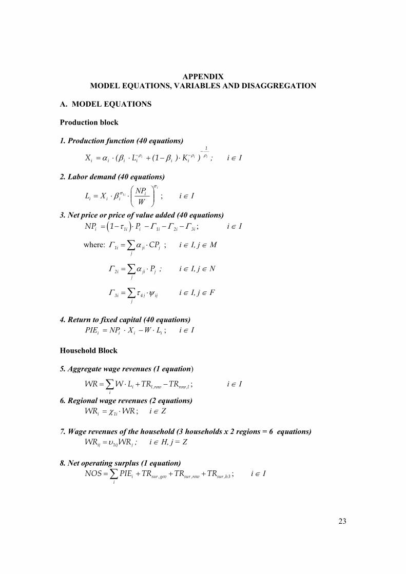
APPENDIX MODEL EQUATIONS, VARIABLES AND DISAGGREGATION

A. MODEL EQUATIONS Production block 1. Production function (40 equations)

i i i

1

i i i i i iX ( L (1 ) K )ρ ρ ρα β β−

− −= ⋅ ⋅ + − ⋅ ; i ∈ I 2. Labor demand (40 equations)

i

i

WNPXL i

iii

σσβ

⋅⋅= 1 ; i ∈ I

3. Net price or price of value added (40 equations) ( )i 1i i 1i 2i 3iNP 1 Pτ Γ Γ Γ= − ⋅ − − − ; i ∈ I

where: 1i ji jj

CPΓ α= ⋅∑ ; i ∈ I, j ∈ M

2i ji jj

PΓ α= ⋅∑ ; i ∈ I, j ∈ N

3i 4 j ijj

Γ τ ψ= ⋅∑ i ∈ I, j ∈ F

4. Return to fixed capital (40 equations)

iiii LWXNPPIE ⋅−⋅= ; i ∈ I Household Block 5. Aggregate wage revenues (1 equation)

i l ,row row,li

WR W L TR TR= ⋅ + −∑ ; i ∈ I

6. Regional wage revenues (2 equations) i 1iWR WRχ= ⋅ ; i ∈ Z

7. Wage revenues of the household (3 households x 2 regions = 6 equations)

ij 1ij jWR WRυ= ; i ∈ H, j = Z 8. Net operating surplus (1 equation)

i sur ,gov sur ,row sur ,h3i

NOS PIE TR TR TR= + + +∑ ; i ∈ I

24

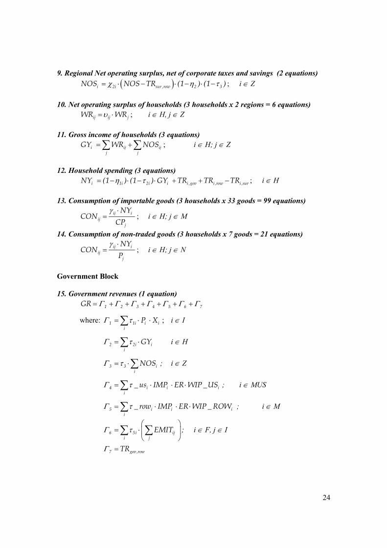
9. Regional Net operating surplus, net of corporate taxes and savings (2 equations) ( )i 2i sur ,row 2 3NOS NOS TR (1 ) (1 )χ η τ= ⋅ − ⋅ − ⋅ − ; i ∈ Z

10. Net operating surplus of households (3 households x 2 regions = 6 equations)

ij ij jWR WRυ= ⋅ ; i ∈ H, j ∈ Z 11. Gross income of households (3 equations)

i ij ijj j

GY WR NOS= +∑ ∑ ; i ∈ H; j ∈ Z

12. Household spending (3 equations)

i 1i 2i i i ,gov i ,row i ,surNY (1 ) (1 ) GY TR TR TRη τ= − ⋅ − ⋅ + + − ; i ∈ H 13. Consumption of importable goods (3 households x 33 goods = 99 equations)

ij iij

j

NYCON

CPγ ⋅

= ; i ∈ H; j ∈ M

14. Consumption of non-traded goods (3 households x 7 goods = 21 equations) ij i

ijj

NYCON

Pγ ⋅

= ; i ∈ H; j ∈ N

Government Block 15. Government revenues (1 equation)

1 2 3 4 5 6 7GR Γ Γ Γ Γ Γ Γ Γ= + + + + + +

where: 1 1i i ii

P XΓ τ= ⋅ ⋅∑ ; i ∈ I

2 2i ii

GYΓ τ= ⋅∑ i ∈ H

3 3 ii

NOSΓ τ= ⋅∑ ; i ∈ Z

4 i i ii

_ us IMP ER WIP _USΓ τ= ⋅ ⋅ ⋅∑ ; i ∈ MUS

5 i i ii

_ row IMP ER WIP _ ROWΓ τ= ⋅ ⋅ ⋅∑ ; i ∈ M

6 5i iji j

EMITΓ τ

= ⋅

∑ ∑ ; i ∈ F, j ∈ I

7 gov ,rowTRΓ =

25

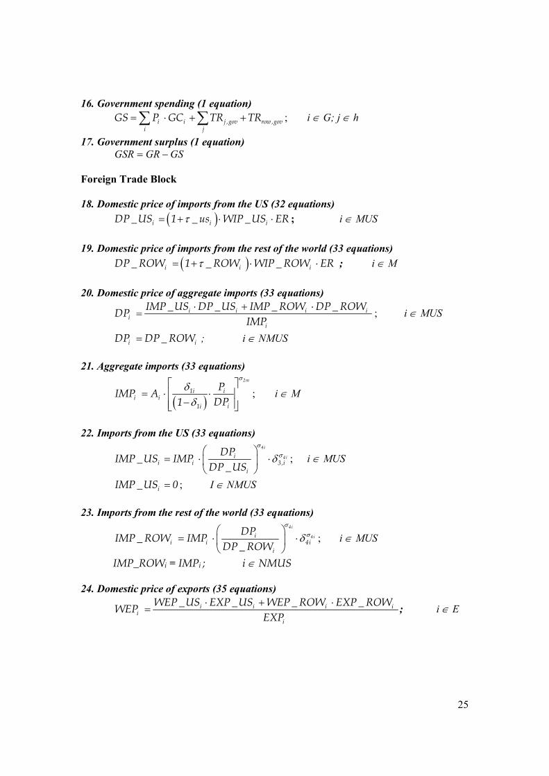
16. Government spending (1 equation) i i j ,gov row ,gov

i jGS P GC TR TR= ⋅ + +∑ ∑ ; i ∈ G; j ∈ h

17. Government surplus (1 equation) GSGRGSR −=

Foreign Trade Block 18. Domestic price of imports from the US (32 equations)

( )i i iDP _US 1 _ us WIP _US ERτ= + ⋅ ⋅ ; i ∈ MUS 19. Domestic price of imports from the rest of the world (33 equations)

( )i i iDP _ ROW 1 _ ROW WIP _ ROW ERτ= + ⋅ ⋅ ; i ∈ M 20. Domestic price of aggregate imports (33 equations)

i i i ii

i

IMP _US DP _US IMP _ ROW DP _ ROWDPIMP

⋅ + ⋅= ; i ∈ MUS

i iDP DP _ ROW= ; i ∈ NMUS

21. Aggregate imports (33 equations)

( )

2m

1i ii i

i1i

PIMP ADP1

σ

δδ

= ⋅ ⋅

− ; i ∈ M

22. Imports from the US (33 equations)

4i

4 iii i 3 ,i

i

DPIMP _US IMPDP _US

σσδ

= ⋅ ⋅

; i ∈ MUS

iIMP _US 0= ; I ∈ NMUS 23. Imports from the rest of the world (33 equations)

4i

4 iii i 4i

i

DPIMP _ ROW IMPDP _ ROW

σσδ

= ⋅ ⋅

; i ∈ MUS

IMP_ROWi = IMPi ; i ∈ NMUS 24. Domestic price of exports (35 equations)

i i i ii

i

WEP _US EXP _US WEP _ ROW EXP _ ROWWEPEXP

⋅ + ⋅= ; i ∈ E

26

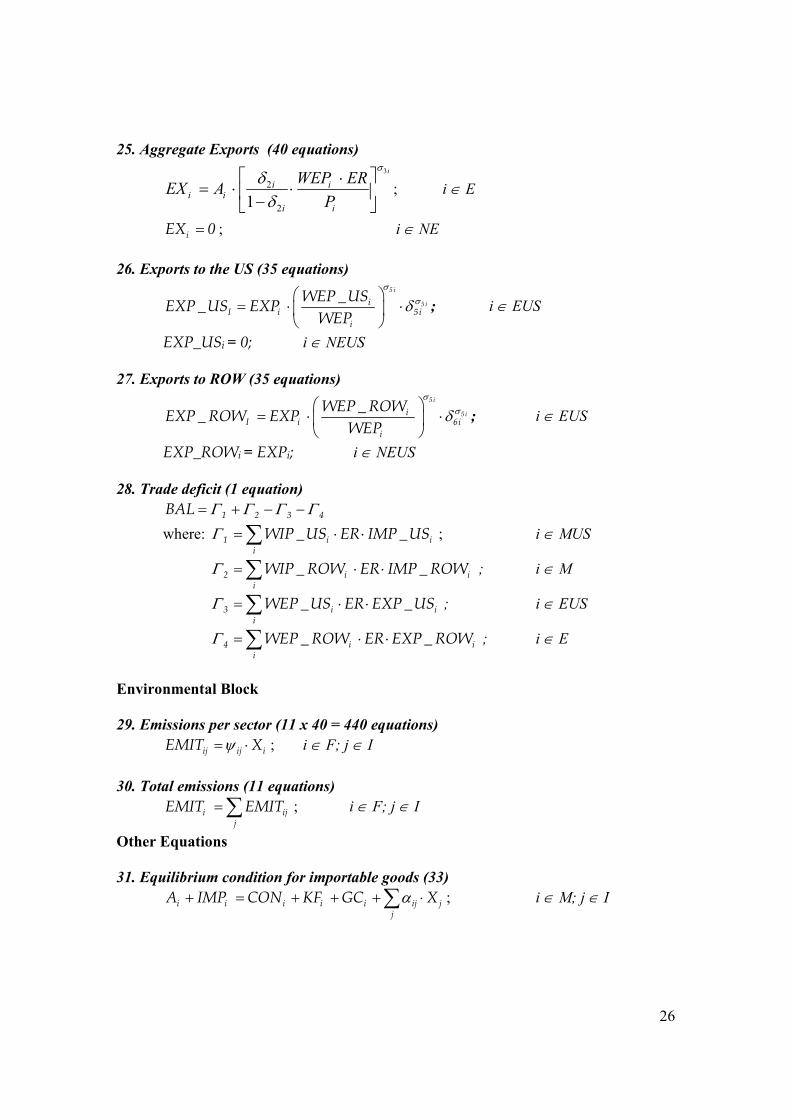
25. Aggregate Exports (40 equations) 3

2

21

σδ

δ ⋅

= ⋅ ⋅ −

i

i ii i

i i

WEP EREX AP

; i ∈ E

iEX 0= ; i ∈ NE 26. Exports to the US (35 equations)

5 i

5 iiI i 5i

i

WEP _USEXP _US EXPWEP

σσδ

= ⋅ ⋅

; i ∈ EUS

EXP_USi = 0; i ∈ NEUS 27. Exports to ROW (35 equations)

5 i

5 iiI i 6i

i

WEP _ ROWEXP _ ROW EXPWEP

σσδ

= ⋅ ⋅

; i ∈ EUS

EXP_ROWi = EXPi; i ∈ NEUS 28. Trade deficit (1 equation)

1 2 3 4BAL Γ Γ Γ Γ= + − − where: 1 i i

iWIP _US ER IMP _USΓ = ⋅ ⋅∑ ; i ∈ MUS

2 i ii

WIP _ ROW ER IMP _ ROWΓ = ⋅ ⋅∑ ; i ∈ M

3 i ii

WEP _US ER EXP _USΓ = ⋅ ⋅∑ ; i ∈ EUS

4 i ii

WEP _ ROW ER EXP _ ROWΓ = ⋅ ⋅∑ ; i ∈ E

Environmental Block 29. Emissions per sector (11 x 40 = 440 equations)

ij ij iEMIT Xψ= ⋅ ; i ∈ F; j ∈ I 30. Total emissions (11 equations)

i ijj

EMIT EMIT= ∑ ; i ∈ F; j ∈ I

Other Equations 31. Equilibrium condition for importable goods (33)

i i i i i ij jj

A IMP CON KF GC Xα+ = + + + ⋅∑ ; i ∈ M; j ∈ I

27

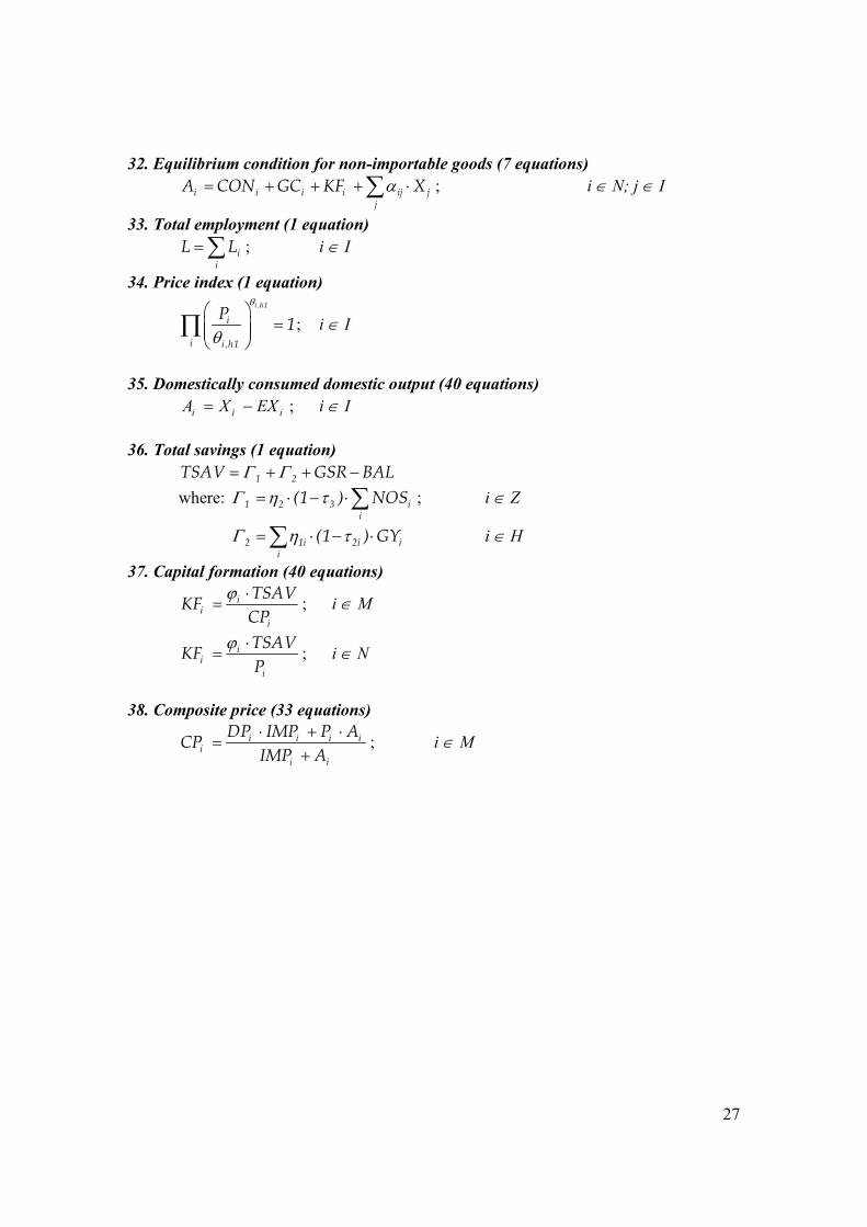
32. Equilibrium condition for non-importable goods (7 equations) i i i i ij j

jA CON GC KF Xα= + + + ⋅∑ ; i ∈ N; j ∈ I

33. Total employment (1 equation) i

iL L= ∑ ; i ∈ I

34. Price index (1 equation) i ,h1

i

i i ,h1

P 1θ

θ

=

∏ ; i ∈ I

35. Domestically consumed domestic output (40 equations)

iii EXXA −= ; i ∈ I 36. Total savings (1 equation)

1 2TSAV GSR BALΓ Γ= + + − where: 1 2 3 i

i(1 ) NOSΓ η τ= ⋅ − ⋅∑ ; i ∈ Z

2 1i 2i ii

(1 ) GYΓ η τ= ⋅ − ⋅∑ i ∈ H

37. Capital formation (40 equations) i

ii

TSAVKFCP

ϕ ⋅= ; i ∈ M

ii

i

TSAVKFP

ϕ ⋅= ; i ∈ N

38. Composite price (33 equations)

i i i ii

i i

DP IMP P ACPIMP A⋅ + ⋅

=+

; i ∈ M

28

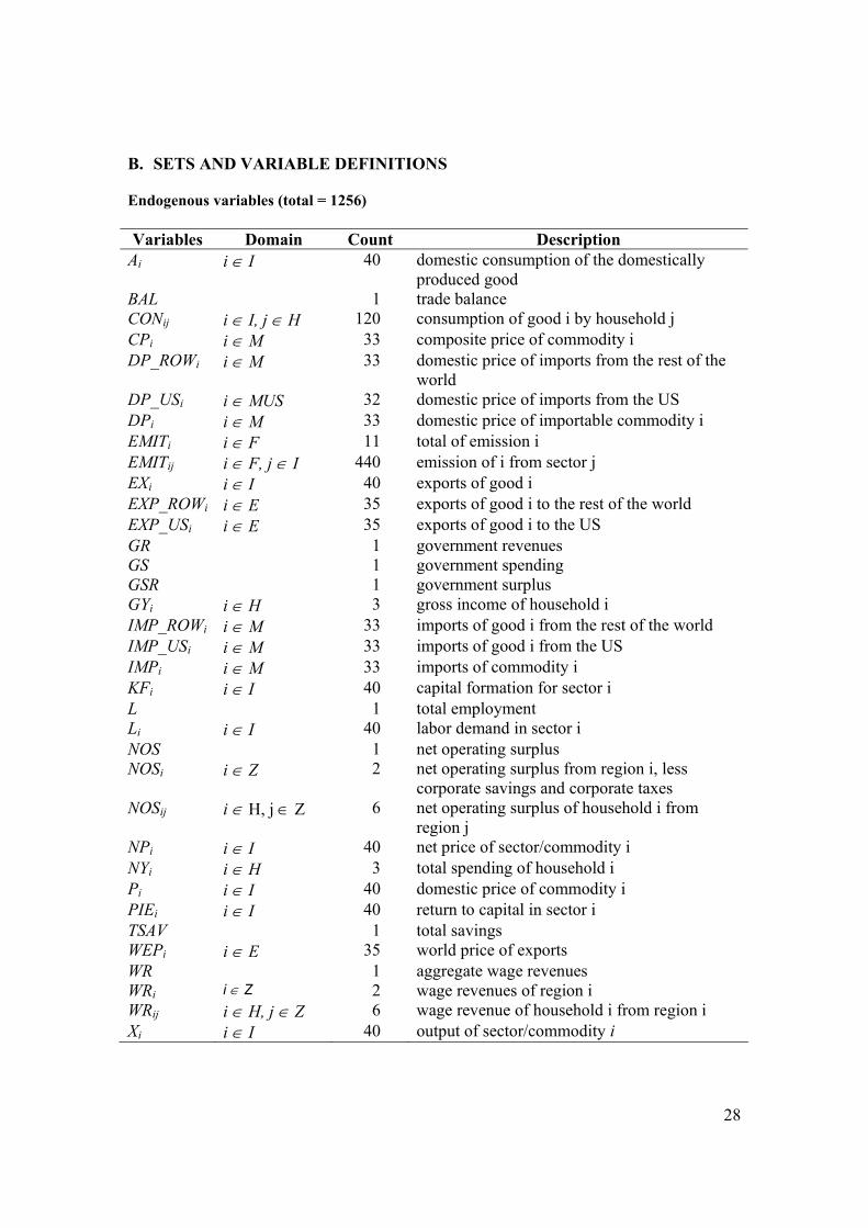
B. SETS AND VARIABLE DEFINITIONS Endogenous variables (total = 1256) Variables Domain Count Description

Ai i ∈ I 40 domestic consumption of the domestically produced good

BAL 1 trade balance CONij i ∈ I, j ∈ H 120 consumption of good i by household j CPi i ∈ M 33 composite price of commodity i DP_ROWi i ∈ M 33 domestic price of imports from the rest of the

world DP_USi i ∈ MUS 32 domestic price of imports from the US DPi i ∈ M 33 domestic price of importable commodity i EMITi i ∈ F 11 total of emission i EMITij i ∈ F, j ∈ I 440 emission of i from sector j EXi i ∈ I 40 exports of good i EXP_ROWi i ∈ E 35 exports of good i to the rest of the world EXP_USi i ∈ E 35 exports of good i to the US GR 1 government revenues GS 1 government spending GSR 1 government surplus GYi i ∈ H 3 gross income of household i IMP_ROWi i ∈ M 33 imports of good i from the rest of the world IMP_USi i ∈ M 33 imports of good i from the US IMPi i ∈ M 33 imports of commodity i KFi i ∈ I 40 capital formation for sector i L 1 total employment Li i ∈ I 40 labor demand in sector i NOS 1 net operating surplus NOSi i ∈ Z 2 net operating surplus from region i, less

corporate savings and corporate taxes NOSij i ∈ H, j ∈ Z 6 net operating surplus of household i from

region j NPi i ∈ I 40 net price of sector/commodity i NYi i ∈ H 3 total spending of household i Pi i ∈ I 40 domestic price of commodity i PIEi i ∈ I 40 return to capital in sector i TSAV 1 total savings WEPi i ∈ E 35 world price of exports WR 1 aggregate wage revenues WRi i ∈ Z 2 wage revenues of region i WRij i ∈ H, j ∈ Z 6 wage revenue of household i from region i Xi i ∈ I 40 output of sector/commodity i

29

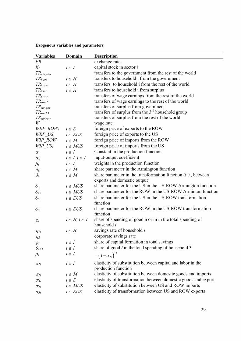
Exogenous variables and parameters Variables Domain Description ER exchange rate Ki i ∈ I capital stock in sector i TRgov,row transfers to the government from the rest of the world TRi,gov i ∈ H transfers to household i from the government TRi,row i ∈ H transfers to household i from the rest of the world TRi,sur i ∈ H transfers to household i from surplus TRl,row transfers of wage earnings from the rest of the world TRrow,l transfers of wage earnings to the rest of the world TRsur,gov transfers of surplus from government TRsur,h3 transfers of surplus from the 3rd household group TRsur,row transfers of surplus from the rest of the world W wage rate WEP_ROWi i ∈ E foreign price of exports to the ROW WEP_USi i ∈ EUS foreign price of exports to the US WIP_ROWi i ∈ M foreign price of imports from the ROW WIP_USi i ∈ MUS foreign price of imports from the US αi i ∈ I Constant in the production function αij i ∈ I, j ∈ I input-output coefficient βi i ∈ I weights in the production function δ1i i ∈ M share parameter in the Armington function δ2i i ∈ M share parameter in the transformation function (i.e., between

exports and domestic output) δ3i i ∈ MUS share parameter for the US in the US-ROW Armington function δ4i i ∈ MUS share parameter for the ROW in the US-ROW Arminton function δ5i i ∈ EUS share parameter for the US in the US-ROW transformation

function δ6i i ∈ EUS share parameter for the ROW in the US-ROW transformation

function γij i ∈ H, i ∈ I share of spending of good n or m in the total spending of

household i η1i i ∈ H savings rate of household i η2 corporate savings rate ϕi i ∈ I share of capital formation in total savings θi,h3 i ∈ I share of good i in the total spending of household 3 ρi i ∈ I ( ) 1

1i1 σ−

= −

σ1i i ∈ I elasticity of substitution between capital and labor in the production function

σ2i i ∈ M elasticity of substitution between domestic goods and imports σ3i i ∈ E elasticity of transformation between domestic goods and exports σ4i i ∈ MUS elasticity of substitution between US and ROW imports σ5i i ∈ EUS elasticity of transformation between US and ROW exports

30

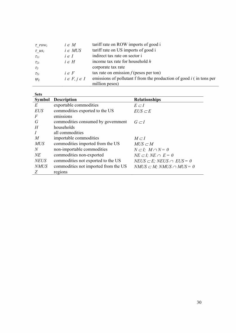
τ_rowi i ∈ M tariff rate on ROW imports of good i τ_usi i ∈ MUS tariff rate on US imports of good i τ1i i ∈ I indirect tax rate on sector i τ2i i ∈ H income tax rate for household h τ3 corporate tax rate τ5i i ∈ F tax rate on emission f (pesos per ton) ψij i ∈ F, j ∈ I emissions of pollutant f from the production of good i ( in tons per

million pesos) Sets Symbol Description Relationships E exportable commodities E ⊂ I EUS commodities exported to the US EUS ⊂ E F emissions G commodities consumed by government G ⊂ I H households I all commodities M importable commodities M ⊂ I MUS commodities imported from the US MUS ⊂ M N non-importable commodities N ⊂ I; M ∩ N = 0 NE commodities non-exported NE ⊂ I; NE ∩ E = 0 NEUS commodities not exported to the US NEUS ⊂ E; NEUS ∩ EUS = 0 NMUS commodities not imported from the US NMUS ⊂ M; NMUS ∩ MUS = 0 Z regions

31

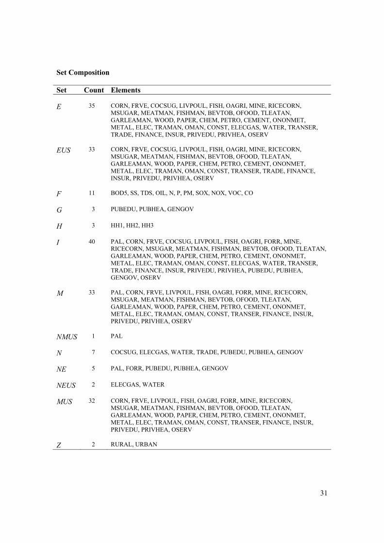
Set Composition Set Count Elements

E 35 CORN, FRVE, COCSUG, LIVPOUL, FISH, OAGRI, MINE, RICECORN, MSUGAR, MEATMAN, FISHMAN, BEVTOB, OFOOD, TLEATAN, GARLEAMAN, WOOD, PAPER, CHEM, PETRO, CEMENT, ONONMET, METAL, ELEC, TRAMAN, OMAN, CONST, ELECGAS, WATER, TRANSER, TRADE, FINANCE, INSUR, PRIVEDU, PRIVHEA, OSERV

EUS 33 CORN, FRVE, COCSUG, LIVPOUL, FISH, OAGRI, MINE, RICECORN, MSUGAR, MEATMAN, FISHMAN, BEVTOB, OFOOD, TLEATAN, GARLEAMAN, WOOD, PAPER, CHEM, PETRO, CEMENT, ONONMET, METAL, ELEC, TRAMAN, OMAN, CONST, TRANSER, TRADE, FINANCE, INSUR, PRIVEDU, PRIVHEA, OSERV

F 11 BOD5, SS, TDS, OIL, N, P, PM, SOX, NOX, VOC, CO

G 3 PUBEDU, PUBHEA, GENGOV

H 3 HH1, HH2, HH3

I 40 PAL, CORN, FRVE, COCSUG, LIVPOUL, FISH, OAGRI, FORR, MINE, RICECORN, MSUGAR, MEATMAN, FISHMAN, BEVTOB, OFOOD, TLEATAN, GARLEAMAN, WOOD, PAPER, CHEM, PETRO, CEMENT, ONONMET, METAL, ELEC, TRAMAN, OMAN, CONST, ELECGAS, WATER, TRANSER, TRADE, FINANCE, INSUR, PRIVEDU, PRIVHEA, PUBEDU, PUBHEA, GENGOV, OSERV

M 33 PAL, CORN, FRVE, LIVPOUL, FISH, OAGRI, FORR, MINE, RICECORN, MSUGAR, MEATMAN, FISHMAN, BEVTOB, OFOOD, TLEATAN, GARLEAMAN, WOOD, PAPER, CHEM, PETRO, CEMENT, ONONMET, METAL, ELEC, TRAMAN, OMAN, CONST, TRANSER, FINANCE, INSUR, PRIVEDU, PRIVHEA, OSERV

NMUS 1 PAL

N 7 COCSUG, ELECGAS, WATER, TRADE, PUBEDU, PUBHEA, GENGOV

NE 5 PAL, FORR, PUBEDU, PUBHEA, GENGOV

NEUS 2 ELECGAS, WATER

MUS 32 CORN, FRVE, LIVPOUL, FISH, OAGRI, FORR, MINE, RICECORN, MSUGAR, MEATMAN, FISHMAN, BEVTOB, OFOOD, TLEATAN, GARLEAMAN, WOOD, PAPER, CHEM, PETRO, CEMENT, ONONMET, METAL, ELEC, TRAMAN, OMAN, CONST, TRANSER, FINANCE, INSUR, PRIVEDU, PRIVHEA, OSERV

Z 2 RURAL, URBAN

32

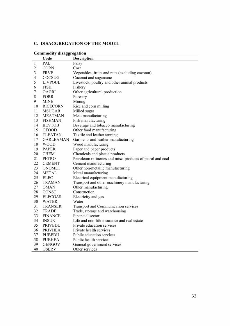
C. DISAGGREGATION OF THE MODEL

Commodity disaggregation Code Description 1 PAL Palay 2 CORN Corn 3 FRVE Vegetables, fruits and nuts (excluding coconut) 4 COCSUG Coconut and sugarcane 5 LIVPOUL Livestock, poultry and other animal products 6 FISH Fishery 7 OAGRI Other agricultural production 8 FORR Forestry 9 MINE Mining 10 RICECORN Rice and corn milling 11 MSUGAR Milled sugar 12 MEATMAN Meat manufacturing 13 FISHMAN Fish manufacturing 14 BEVTOB Beverage and tobacco manufacturing 15 OFOOD Other food manufacturing 16 TLEATAN Textile and leather tanning 17 GARLEAMAN Garments and leather manufacturing 18 WOOD Wood manufacturing 19 PAPER Paper and paper products 20 CHEM Chemicals and plastic products 21 PETRO Petroleum refineries and misc. products of petrol and coal 22 CEMENT Cement manufacturing 23 ONOMET Other non-metallic manufacturing 24 METAL Metal manufacturing 25 ELEC Electrical equipment manufacturing 26 TRAMAN Transport and other machinery manufacturing 27 OMAN Other manufacturing 28 CONST Construction 29 ELECGAS Electricity and gas 30 WATER Water 31 TRANSER Transport and Communication services 32 TRADE Trade, storage and warehousing 33 FINANCE Financial sector 34 INSUR Life and non-life insurance and real estate 35 PRIVEDU Private education services 36 PRIVHEA Private health services 37 PUBEDU Public education services 38 PUBHEA Public health services 39 GENGOV General government services 40 OSERV Other services

33

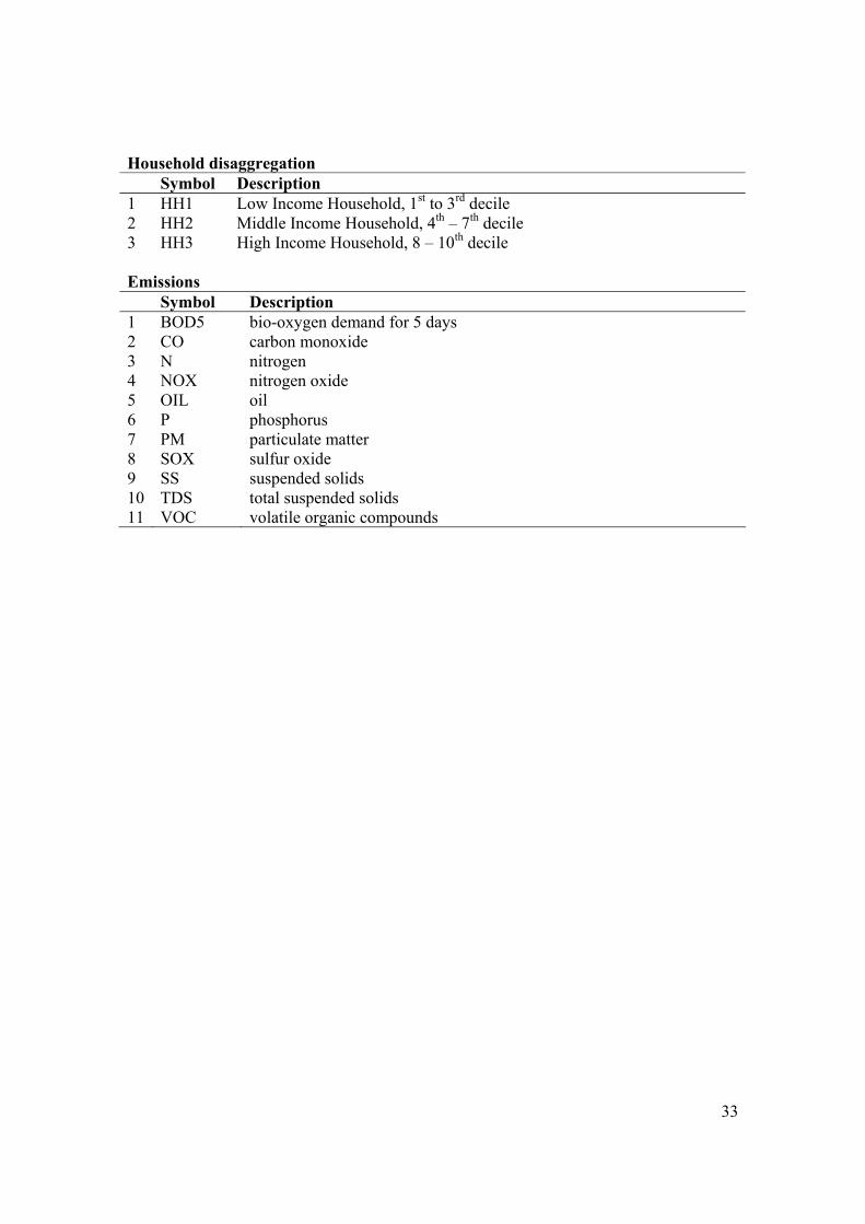
Household disaggregation Symbol Description 1 HH1 Low Income Household, 1st to 3rd decile 2 HH2 Middle Income Household, 4th – 7th decile 3 HH3 High Income Household, 8 – 10th decile Emissions Symbol Description 1 BOD5 bio-oxygen demand for 5 days 2 CO carbon monoxide 3 N nitrogen 4 NOX nitrogen oxide 5 OIL oil 6 P phosphorus 7 PM particulate matter 8 SOX sulfur oxide 9 SS suspended solids 10 TDS total suspended solids 11 VOC volatile organic compounds