The Immersed Boundary Method - monsite-1 · Turbine blades are exposed to ... case the thermal load is generated ... The primary advantage of the immersed boundary method is associated

The Immersed Boundary Method

Gianluca IaccarinoMechanical Engineering Department

Institute for Computational Mathematical EngineeringStanford University

Notes prepared for a Short Course offered at the University of Bordeaux and INRIA in January 2016, in theframework of the Aquarius project in collaboration between INRIA Bordeaux and Stanford University.

Acknowledgements

I wish to extend my gratitude to many colleagues that worked with me on the development of the numericalmethods and algorithms described in these notes. In particular, I thank R. Verzicco, M. De Tullio, S. Kang, F.Ham, R. Mittal, S. Moreau, G. Kalitzin, S. Das and D. Cook.

Disclaimer

This is a draft version of the Lecture Notes. I apologize for typing errors and omissions - particularly with thereferences; these will be fixed in the final version on the notes. Please send an email to [email protected] withcorrections and comments.

2

Contents

1 Introduction 5

2 Immersed Boundary Method 92.1 Imposition of Boundary Conditions . . . . . . . . . . . . . . . . . . . . . . . . . . . . . . . . . . 112.2 Continuous Forcing Approach . . . . . . . . . . . . . . . . . . . . . . . . . . . . . . . . . . . . . 12

2.2.1 Flows with Elastic Boundaries . . . . . . . . . . . . . . . . . . . . . . . . . . . . . . . . 122.2.2 Flows with Rigid Boundaries . . . . . . . . . . . . . . . . . . . . . . . . . . . . . . . . . 132.2.3 General considerations . . . . . . . . . . . . . . . . . . . . . . . . . . . . . . . . . . . . . 14

2.3 Discrete Forcing Approach . . . . . . . . . . . . . . . . . . . . . . . . . . . . . . . . . . . . . . 142.3.1 Indirect BC Imposition . . . . . . . . . . . . . . . . . . . . . . . . . . . . . . . . . . . . 152.3.2 Direct BC Imposition . . . . . . . . . . . . . . . . . . . . . . . . . . . . . . . . . . . . . 152.3.3 General Considerations . . . . . . . . . . . . . . . . . . . . . . . . . . . . . . . . . . . . 17

2.4 Flows with Moving Boundaries . . . . . . . . . . . . . . . . . . . . . . . . . . . . . . . . . . . . 172.5 Examples of applications . . . . . . . . . . . . . . . . . . . . . . . . . . . . . . . . . . . . . . . 18

2.5.1 Channel flow with a rigid membrane . . . . . . . . . . . . . . . . . . . . . . . . . . . . . 182.5.2 Flow Past Flapping Filaments . . . . . . . . . . . . . . . . . . . . . . . . . . . . . . . . . 20

3 Geometry and Grid Generation 233.1 Geometry Definition . . . . . . . . . . . . . . . . . . . . . . . . . . . . . . . . . . . . . . . . . . 243.2 Grid Generation . . . . . . . . . . . . . . . . . . . . . . . . . . . . . . . . . . . . . . . . . . . . 25

3.2.1 Ray tracing . . . . . . . . . . . . . . . . . . . . . . . . . . . . . . . . . . . . . . . . . . 273.3 Grid Refinement . . . . . . . . . . . . . . . . . . . . . . . . . . . . . . . . . . . . . . . . . . . . 28

3.3.1 Anisotropic grid refinement . . . . . . . . . . . . . . . . . . . . . . . . . . . . . . . . . . 293.3.2 Grid Smoothing . . . . . . . . . . . . . . . . . . . . . . . . . . . . . . . . . . . . . . . . 29

4 Fluid Flow Simulations 314.1 The Unstructured Navier-Stokes Solver . . . . . . . . . . . . . . . . . . . . . . . . . . . . . . . . 32

4.1.1 The Immersed Boundary Reconstruction . . . . . . . . . . . . . . . . . . . . . . . . . . . 334.1.2 Turbulent Channel Flow . . . . . . . . . . . . . . . . . . . . . . . . . . . . . . . . . . . . 354.1.3 Flow Past Spheres . . . . . . . . . . . . . . . . . . . . . . . . . . . . . . . . . . . . . . . 36

5 Solid/Fluid Thermal Coupling 395.1 The Numerical method . . . . . . . . . . . . . . . . . . . . . . . . . . . . . . . . . . . . . . . . 39

5.1.1 Description of the immersed boundary-approximated domain method (IB-ADM) . . . . . . 405.1.2 Implementation for a multi-material problem (conjugate heat transfer) . . . . . . . . . . . 42

5.2 Verification study . . . . . . . . . . . . . . . . . . . . . . . . . . . . . . . . . . . . . . . . . . . 445.2.1 Flow around a heated sphere . . . . . . . . . . . . . . . . . . . . . . . . . . . . . . . . . 445.2.2 Accuracy of the IB method for conjugate heat transfer . . . . . . . . . . . . . . . . . . . 45

5.3 A heated cylinder in a channel heated from below . . . . . . . . . . . . . . . . . . . . . . . . . . 465.3.1 Experimental configuration . . . . . . . . . . . . . . . . . . . . . . . . . . . . . . . . . . 465.3.2 Computational setup . . . . . . . . . . . . . . . . . . . . . . . . . . . . . . . . . . . . . 475.3.3 Effect of grid resolution . . . . . . . . . . . . . . . . . . . . . . . . . . . . . . . . . . . . 475.3.4 Results with conjugate heat transfer . . . . . . . . . . . . . . . . . . . . . . . . . . . . . 515.3.5 Effects of the Boussinesq approximation and constant material properties . . . . . . . . . 51

6 Applications 556.1 Electronic Component Unit . . . . . . . . . . . . . . . . . . . . . . . . . . . . . . . . . . . . . . 556.2 Electric Motors . . . . . . . . . . . . . . . . . . . . . . . . . . . . . . . . . . . . . . . . . . . . 57

7 Supplementary Material 59

3

1Introduction

In the design process of many engineering systems, one increasingly important problem is the interaction ofthe components which might lead to structural, thermal and aerodynamic performance thresholds. One classicalexample, are the turbine blades in modern gas-turbine engine, which operate at high combustor outlet temperaturesof 1300 − 1500oC, to achieve higher thermal efficiency and thrust. Turbine blades are exposed to these high-temperature gases and undergo severe thermal stress and fatigue. The design of highly efficient cooling systemsfor turbine blades has an enormous potential impact on the overall market value of modern engines. Coolingdevices are based on a secondary flow system built into each blade (see Fig. 1.1). The secondary flow passagesare extremely complicated consisting of one or multiple legs with turbulators (rib-roughened serpentines), holesconnecting the secondary path to the external surface of the blade (film cooling), tube bundles, slots, etc.

Figure 1.1: Turbine blade with secondary cooling passages

5

CHAPTER 1. INTRODUCTION

Figure 1.2: Wall Thermal Conditions: (a) rib insu-lated, (b) solid-fluid simulation, constant heat fluxat the base of the rib, (c) constant heat flux at therib surface

Figure 1.3: Temperature distribution in the vicinityof the rib. Left) Effect of the wall thermal condi-tion; (a) heated rib, (b) solid-fluid coupling and (c)insulated rib. Right) Effect of the rib thermal con-ductivity: (a) ks/kf = 100, (b) kf = ks and (c)kf/ks = 100.

Today, the design of turbine blades is approached with a combination of experiments and numerical analysis.Most numerical simulations, though, rely on simple thermal boundary conditions (fixed temperature or heat flux)to evaluate the heat transfer characteristics of cooling devices. In realistic operating conditions, the overall surfacethermal state is the result of an energy balance between convection and conduction in the fluid and in the solidand, therefore, accurate predictions of the heat transfer rates require the solution of the coupled solid/fluid heattransfer problem.

As a demonstration of such important solid/fluid coupling a simple example illustrating the heat transfer ina ribbed channel typical of secondary cooling passages in turbine blades is summarized. Three simulations areconsidered: these are summarized in Fig. 1.2 and correspond to insulated rib, coupled solid/fluid analysis (noboundary condition is required at the interface) and constant heat flux at the rib surface. The thermal fieldis assumed to be uncoupled from the velocity field and therefore only the temperature distributions must becompared. In Fig. 1.3 temperature contours in the vicinity of the rib are reported. The dark area in the figurecorresponds to lower temperatures – and, thus, to higher Nusselt numbers on the surface. The conjugate heattransfer calculation of Fig. 1.3 (b) is for the same conductivity of the fluid and the solid (kf = ks). The qualitativeand quantitative features of the solution corresponding to the solid-fluid coupled thermal field (Fig. 1.3 (b)) arein between the adiabatic (Fig. 1.3 (c)) and prescribed heat flux (Fig. 1.3 (a)) cases. Data in Fig. 1.3 showthat the region downstream of the rib is not dramatically affected by the various thermal boundary conditions.On the other hand, the area upstream of the rib shows large differences: when the rib side wall is heated, thefluid that impinges in the channel floor is approximately at the same temperature as the wall. When the siderib wall is adiabatic (see Fig. 1.3 (c)), cold fluid reaches the floor and correspondingly high levels of Nu arepredicted. The effect of varying the rib thermal conductivity (ks) is investigated in Fig. ??. Temperature fieldscorresponding to high and low conductivity are reported in the figure. The upstream region does not show astrong dependency on ks because the heat transfer is dominated by convection. The downstream region, on theother hand, is dramatically changed because, near the rib, heat is removed from the fluid mainly by conduction.

This is further illustrated by the surface Nusselt number (Fig. 1.4). The two limiting conditions of insulatedand heated ribs show nearly the same levels of heat transfer in the downstream region. Upstream, as noted

6

previously, cold fluid reaches the floor when the rib side wall is not heated. The analysis of the conjugate heattransfer predictions shows that conduction plays a major role in the downstream area. Results at other Reynoldsnumbers are consistent with this observation.

The level of the heat transfer away from the rib is only slightly altered by the rib boundary condition. This givesconfidence in the good agreement with the measurements presented in the previous sections. On the other hand,the differences in the vicinity of the ribs are substantial. Hence, differences observed between the experimentaldata in Fig. ?? could be related to differences between the experimental set-ups. Fig. 1.4 illustrates that clearlyprescribed surface conditions are needed in order to accurately test numerical predictions on the wall adjacent tothe rib.

Figure 1.4: Nusselt number on the floor of the chan-nel. Effect of the wall thermal condition and the ribconductivity. Insulated rib, heated rib, ks/kf = 100, kf = ks and kf/ks = 100.

Turbine blades are obviously not the only system is whichcoupling between multiple thermal transfer modes is active.Design of cooling strategies for electronic component is alsoreceiving increasing attention due to the enhanced performanceand the miniaturization requirements. As example of a Elec-tronic Component Unit (ECU) is reported in Fig. 1.5. In thiscase the thermal load is generated mainly in the diodes byJoule heating and might affect the operation of the neighbor-ing electronic components. Natural convection is often notsufficient to control of the temperature and forced convectionbecomes required. In this situation again a multimodal heattransfer analysis is required, in which multiple parts (with dif-ferent material properties) are coupled to establish the overallthermal conditions.

Conventional simulation techniques, based on body-fittedgrids provides capabilities of performing conjugate heat trans-fer analysis (CHT) but several outstanding issues emerge. Thetransfer of extremely complex geometrical models requires con-siderable user intervention even when direct interfaces betweenthe CAD and grid generation software are available. The sur-face representation has very different meanings in CAD andCFD environments. In the former, it the end product andserves as basis for manufacturing. The surfaces are typicallyconverted to a set of points to drive a CAM machine or to a set of triangles for rapid-prototyping manufacturing.The distribution of the output points (or the size of the triangles) is typically based on surface curvature and itis directly controlled by the user in the CAD system. In a CFD environment, the surface representation is onlya starting point and it is used as a support for the surface mesh generation procedure. Once this surface meshis obtained, the volume mesh is built to allow for a CFD solution. There are several constraints on the surfacemesh that make the direct use of CAD surfaces nearly impossible; the most important is the quality of the meshelements. Usually, the CAD model is broken into several smaller components and surface meshes are generatedin patches enforcing quality constraints.

Another important consideration in CHT simulation is the requirement of creating meshes for both the fluidand the solid domains. In addition, to the complexity already illustrated, the need to create a proper interfaceto correctly transfer the thermal fluxes pose additional challenges. Non-conformal interfaces - in which meshesare generated independently on the solid and fluid surfaces are attractive because they decouple the two gridgeneration problems, but can lead to inaccurate transfer and lack of conservation properties. On the other hand,the creation of a common interface mesh poses an addition burden on the mesh generation procedure.

Therefore, the grid generation for a complex geometry, such as a turbine blade, is extremely time consumingand requires very skilled users. This step can represent sometimes more than 80% of the time devoted to astudy. Moreover, in a typical design cycle several parametric studies must be carried out to evaluate the effectof various design solution. This can hardly be done within typical time constraints due to the grid reconstructionstep required for each new simulation. Current industrial practice is to use simplified model problems and toextrapolate the results to build several initial prototypes that are consequently tested. However, such procedurescan hardly yield an optimized system and can be still very costly.

In these lectures, an alternative approach based on the Immersed Boundary technique is proposed to overcome

7

CHAPTER 1. INTRODUCTION

Figure 1.5: Electronic Component Unit (ECU), Courtesy of Bosch

most of the above simulation obstacles. The method is based on the use of Cartesian grids non-conforming withthe physical boundaries. Special algorithmic modifications are added at the interfaces to enforce the boundaryconstraints.

8

2Immersed Boundary Method

The term “immersed boundary method" was first used in reference to a method developed by [78] for simulatingcardiac mechanics and associated blood flow. The distinguishing feature of this method was that the entiresimulation was carried out on a Cartesian grid which did not conform to the geometry of the heart and anovel procedure was formulated for imposing the effect of the immersed boundary on the flow. Since the firstintroduction of this method by Peskin, numerous modifications and refinements have been proposed and therenow exist a number of variants of this approach. In addition, there is another class of methods usually referred toas “Cartesian grid methods" which were originally developed for simulating inviscid flows with complex embeddedsolid boundaries on Cartesian grids ([53]; [99]; [49]). These methods have also been extended to simulate unsteadyviscous flows ([90]; [Ye et al.(1999)]) and as such have capabilities similar to those of immersed boundary methods.For the purposes of this thesis, we will use the term immersed boundary (IB) method to encompass all such methodsthat simulate viscous flows with immersed (or embedded) boundaries on grids that do not conform to the shapeof these boundaries. Furthermore, this introduction will focus mainly on IB methods for flows with immersed solidboundaries. Application of these and related methods to problems with fluid-fluid and fluid-gas boundaries hasbeen covered in the literature [45] and [85].

Consider the simulation of flow past a solid body shown in Figure 2.1(a). The conventional approach to thiswould employ structured or unstructured grids that conform to the body. The generation of these grids proceedsin two sequential steps. First, a surface grid covering the immersed boundary Γb is generated. This is thenused as a boundary condition to generate a grid in the volume Ωf occupied by the fluid. If a finite-differencemethod is employed on a structured grid, then the differential form of the governing equations is transformed toa curvilinear coordinate system aligned with the grid lines ([57]). Since the grid conforms to surface of the body,the transformed equations can then be discretized in the computational domain with relative ease. If a finite-volume technique is employed, then the integral form of the governing equations is discretized and the geometricalinformation regarding the grid is incorporated directly into the discretization. If an unstructured grid is employed,then either a finite-volume or a finite-element methodology can be used. Both approaches incorporate the localcell geometry into the discretization and do not resort to grid transformations.

Now consider employing a non-body conformal Cartesian grid for this simulation as shown in Figure 2.1(b). Inthis approach the immersed boundary would still be represented through some means such as a surface grid butthe Cartesian volume grid would be generated with no regard to this surface grid. Thus, the solid boundary wouldcut through this Cartesian volume grid. Since the grid does not conform to the solid boundary, incorporation of theboundary conditions would require some modification to the equations in the vicinity of the boundary. Preciselywhat these modifications are will be the subject of a detailed discussion in subsequent sections. However, assumingthat such a procedure is available, the governing equations would then be discretized using a finite-difference,finite-volume or a finite-element technique without resorting to coordinate transformation or complex discretizationoperators.

9

CHAPTER 2. IMMERSED BOUNDARY METHOD

(a) (b)

Figure 2.1: (a) Schematic showing a generic body past which flow is to be simulated. The body occupies thevolume Ωb with boundary Γb. The body has a characteristic length scale L, and a boundary layer of thickness δdevelops over the body. (b) Schematic of body immersed in a Cartesian grid on which the governing equationsare discretized.

At this point it is useful to compare the advantages and disadvantages of these two approaches. Clearly,imposition of the boundary conditions is not straightforward in immersed boundary methods and furthermore, theramifications of the boundary treatment on the accuracy and conservation properties of the numerical schemeare not obvious. In addition, alignment between the grid lines and the body surface in body-conformal gridsallows better control of the grid resolution in the vicinity of the body and this has implication for the increasein grid-size with increasing Reynolds number. Consider for example the case of the two-dimensional (2D) bodyof characteristic length L in Figure 2.1(a) with a boundary layer of thickness δ wherein it is required to providean average grid spacing of ∆n and ∆t in the directions normal and tangential to the body surface. It is noweasy to show that for moderately high Reynolds numbers for which δ << L, the size of a body-conformal gridscales as (L/∆t)(δ/∆n) whereas that of a Cartesian grid scales as (L2/∆2

n). Assuming further that ∆n ∝ δ and∆t ∝ L we find that the ratio of sizes for a Cartesian to a body-conformal grid will scale as (L/δ)2. For a laminarboundary layer, (L/δ) ∝ Re0.5 ([86]) which implies that the grid-size ratio will scale with (Re)1.0 for 2D bodies.For a three-dimensional (3D) body, it can be similarly be shown that the grid-size ratio would scale with (Re)1.5.Thus, as the Reynolds number increases, the size of a Cartesian grid increases faster than a corresponding body-conformal grid. It should however be pointed out that this faster increase in grid size does not necessarily imply acorresponding increase in the computational cost since a substantial fraction of the grid points are inside the solidbody where the fluid flow equations need not be solved. Furthermore, in comparison with structured curvilinearbody-formal grids, the use of a Cartesian grid can significantly reduce the per-grid-point operation count due tothe absence of additional terms associated with grid transformations. When compared with unstructured gridmethods, the Cartesian grid based IB method retains the advantage of being amenable to powerful line-iterativetechniques and geometric multigrid methods which can also lead to a low per-grid-point operation count.

The primary advantage of the immersed boundary method is associated with the fact that the task of gridgeneration is greatly simplified. Generation of body-conformal structured or unstructured grid is usually a verycumbersome process. The objective is to construct a grid that provides adequate local resolution with theminimum number of total grid points. For anything but the simplest geometries, these conflicting requirementscan lead to a deterioration in grid-quality which can negatively impact the accuracy as well as the convergenceproperties of the solver ([57]). Thus, even for simple geometries, the generation of a good quality body-conformalgrid can be an iterative process requiring significant input from the person generating the grid. As the geometrybecomes more complicated, the task of generating a acceptable grid becomes increasingly difficult. Within thestructured grid approach, complex geometries are often handled by decomposing the volume into subdomainsand generating a separate grid in each subdomain ([80]). Apart from the complexity that is introduced into thesolution algorithm due to the presence of multiple subdomains, grid smoothness can deteriorate at the interfacebetween subdomains. The unstructured grid approach is inherently better suited for complex geometries buthere too, grid quality can deteriorate with increasing complexity in the geometry. In contrast, for a simulation

10

2.1. IMPOSITION OF BOUNDARY CONDITIONS

carried out on a non-body conformal Cartesian grid, grid complexity and quality is not significantly affected bythe complexity of the geometry.

The advantage of the Cartesian grid based IB method also becomes eminently clear for flows with movingboundaries. Simulation of such flows on body-conformal grids requires the generation of a new grid at eachtime-step as well as a procedure for projecting the solution onto this new grid ([88]). Both of these steps cannegatively impact the simplicity, accuracy, robustness and computational cost of the solution procedure especiallyin cases involving large motions. In contrast, inclusion of body motion in IB methods is relatively simple due tothe use of a stationary, non-deforming Cartesian grid. Thus, despite the significant progress made in simulatingflow with moving boundaries on body-conformal grids ([48]; [88]; [81]), it is fair to say that due to its inherentsimplicity, the IB method represents an extremely attractive alternative for such flows.

2.1 Imposition of Boundary Conditions

Imposition of boundary condition on the immersed boundary is the key factor in the development of an IBalgorithm. It is also what distinguishes one IB method from another. Consider the simulation of incompressibleflow past the body in Figure 2.1(b) which is governed by the following equations:

∂~u

∂t+ ~u · ∇~u+

1

ρ∇p− µ

ρ∇2~u = 0 and

2.1

∇ · ~u = 0 in Ωf ;

with ~u = ~uΓ on Γb, 2.2

where ~u is the the fluid velocity, p is the pressure and ρ and µ the density and viscosity, respectively. The solidbody occupies the domain Ωb with boundary denoted by Γb, and Ωf denotes the surrounding fluid domain. Theouter boundary of the flow domain is disregarded for the purposes of this discussion. For ease of discussion, theabove system can be notionally written as

L(U) = 0 in Ωf 2.3

with U = UΓ on Γb, 2.4

where U = (~u, p) and L is the operator representing the Navier-Stokes equations as in Equation 2.1.Conventional methods proceed by developing a discretization of Equation 2.3 on a body-formal grid where the

boundary condition (2.4) on the immersed boundary Γb is enforced directly. In an IB method, Equation 2.1 wouldbe discretized on a non-body conformal Cartesian grid and the boundary condition imposed indirectly throughsome modification of Equation 2.3. In general, the modification takes the form of a source term (or forcingfunction) in the governing equations which reproduces the effect of boundary. The introduction of a forcingfunction, the precise nature of which will be discussed in the following sections, into the governing equations canbe implemented in two different ways and this leads to a fundamental dichotomy in IB methods. In the firstimplementation, the forcing function, denoted here by f

b, is included into the continuous governing equations 2.3

leading to the equation L(U) = fbwhich then applies to the entire domain (Ωf + Ωb). Note that f

b= (~fm, fp)

where ~fm and fp are the forcing functions applied to the momentum and pressure respectively. This equation issubsequently discretized on a Cartesian grid leading to the following system of discrete equations:

[L] U = fb,

2.5

and this system of equation solved in the entire domain.In the second approach, the governing equations are first discretized on a Cartesian grid without regard to the

immersed boundary resulting in the set of discretized equations [L] U = 0. Following this, the discretizationin the cells near the immersed boundary is adjusted to account for its presence, resulting in a modified systemof equations [L′] U = r which are then solved on the Cartesian grid. In this equation, [L′] is the modifieddiscrete operator and r represents known terms associated with the boundary conditions on the immersedsurface. The above system of equations can be rewritten as

[L] U = f ′b,

2.6

11


where f ′b = r + [L] U − [L′] U. Comparison of Equations 2.5 and 2.6 clearly shows the connection

between the two approaches. In the first approach which we term “continuous forcing approach" the forcing isincorporated into the continuous equations before discretization, whereas in the second approach, which can betermed the “discrete forcing approach," the forcing can be considered to be introduced after the equations havebeen discretized. An attractive feature of the continuous forcing approach is that it is formulated independent ofthe underlying spatial discretization. The discrete forcing approach on the other hand is very much dependent onthe discretization method. However, this allows direct control over the numerical accuracy, stability and discreteconservation properties of the solver. In the following sections we describe methods that fall into each of thesecategories.

2.2 Continuous Forcing Approach

Among existing methods in this category, elastic and rigid boundaries required different treatments and these arediscussed separately in this section.

2.2.1 Flows with Elastic Boundaries

The original IB method by Peskin (1972, 1981) was developed for the coupled simulation of blood flow and musclecontraction in a beating heart and is generally suitable for flows with immersed elastic boundaries. In this methodthe fluid flow is governed by the incompressible Navier-Stokes equations and these are solved on a stationaryCartesian grid. The immersed boundary is represented by a set of elastic fibers and the location of these fibers istracked in a Lagrangian fashion by a collection of massless points that move with the local fluid velocity. Thus,the coordinate ~Xk of the kth Lagrangian point is governed by the equation

∂ ~Xk

∂t= ~u( ~Xk, t)

2.7

The stress (denoted here by ~F ) and deformation of these elastic fibers is related by a constitutive law such as theHooke’s law. The effect of the immersed boundary on the surrounding fluid is essentially captured by transmittingthe fiber stress to the fluid through a localized forcing term in the momentum equations which is given by

~fm(~x, t) =∑k

~Fk(t)δ(|~x− ~Xk|), 2.8

where δ is the Dirac delta function. Since the location of the fibers does not generally coincide with the nodalpoints of the Cartesian grid, the forcing is distributed over a band of cells around each Lagrangian point (seeFigure 2.2(a)) and this distributed force imposed on the momentum equations of the surrounding nodes. Thus,the sharp delta function is essentially replaced by a smoother distribution function, denoted here by d, which issuitable for use on a discrete mesh. The forcing at any grid point xi,j due to the fibers is then given by

~fm(~xi,j , t) =∑k

~Fk(t)d(|~xi,j − ~Xk|). 2.9

The fiber velocity in Equation 2.7 is also obtained through the use of the same smooth function. The choiceof the distribution function d is a key ingredient in this method. Several different distribution functions have beenemployed in the past ([78]; [50]; [84]; [68]) and Figure 2.2(b) shows four such functions.

In [78] original approach the following discrete delta function was used:

δ(r) ≈ dh(r) =1

h

(cos(πr/2h) + 1)/4h, if r ≤ 2h,0 otherwise.

2.10

where r represents the distance between the k − th Lagrangian point representing the surface and any computa-tional cell. As mentioned before, the replacement of δ with dh corresponds to spreading the forcing over severalcells around the fiber.

Other discrete delta functions can be used; the simplest choice is the hat function as used by [84]:

12

2.2. CONTINUOUS FORCING APPROACH

(a) (b)

Figure 2.2: (a) Transfer of forcing ~Fk from Lagrangian boundary point ( ~Xk) to surrounding fluid nodes. Shadedregion signifies the extent of the force distribution. (b) Distribution functions employed in various studies.

δ(r) ≈ dh(r) =1

h

(2h+ r)/4h2, if r ≤ 2h,0 otherwise.

2.11

which corresponds to a simple area weighted average ([68]). More sophisticated functions have been introducedby [50] and recently by [68].

The mathematical analysis of the IB approach carried out by [50] and [69] allows to shed some light on theimportance of the choice of the discrete delta function and provides a link between this approach and generalboundary-capturing discretizations.

[50] studied a simple one-dimensional model problem and carried out an analysis of the accuracy of a nominalsecond-order discretization for various choices of the forcing terms; they also provided guidelines to the formulationof appropriate discrete delta functions. The key element in the analysis is the formal equivalence between theDirac function definition and a general interpolation formula. Using Taylor expansions, [50] proved that the simplediscrete functions (2.10) and (2.11) are second and first order accurate respectively when no discontinuities arepresent at the location of the forcing. A more general function:

δ(r) ≈ dh(r) =1

h

1− (r/h)2, if r ≤ h,2− 3r/h+ (r/h)2, h ≤ r ≤ 2h,0 otherwise.

2.12

is proven to be second-order accurate even when discontinuity are present (but the function is smooth on bothsides). Interestingly, [50] provide an interpretation for (2.12) based on linear extrapolation of the function on bothsides of the discontinuity followed by a convex combination of the two one-sided extrapolation. Recently, [68]introduced a formally second order accurate IB by using a new discrete delta function similar to (2.12).

Methods in this category have been successfully used for a wide variety of problems including cardiac mechanics([79]), cochlear dynamics ([51]), aquatic animal locomotion ([55]), bubble dynamics ([94]) and flow past flexiblefilaments ([101]).

2.2.2 Flows with Rigid BoundariesThe previous method is naturally well suited for elastic bodies but its application to flows with rigid bodies posesproblems since the constitutive laws used for elastic boundaries are not generally well posed in the rigid limit. Thisproblem could be circumvented by considering the body to be still elastic but extremely stiff. A second approachis to consider the structure attached to an equilibrium location ([50]; [68]) by a spring with a restoring force ~Fgiven by:

~Fk(t) = −κ( ~Xk − ~Xek(t))

2.13

where κ is a positive spring constant and ~Xek is the equilibrium location of the kth Lagrangian point. Accurate

imposition of the boundary condition on the rigid immersed boundary requires large values of κ. This however,

13


results in a stiff system of equations which can be subject to severe stability constraints ([87]; [68]). On theother hand, lower values of κ can lead to spurious elastic effects such as excessive deviation from the equilibriumlocation as noted in the low Reynolds cylinder wake simulations of [68].

The above approach can be viewed as a specific version of the model developed by [60] to simulate the flowaround rigid bodies. In this model, the effect of the rigid body on the surrounding flow is modeled through aforcing term

~F (t) = α

∫ t

0

~u(τ)dτ + β~u(t) 2.14

where the coefficients α and β are selected so as to best enforce the boundary condition at the immersed solidboundary. The original intent behind Equation 2.14 was to provide feedback control of the velocity near thesurface ([60]) but from a physical point of view, it can also be viewed as representing a damped oscillator ([61]).This method has been used to simulate startup flow past a circular cylinder at a moderate Reynolds number andlow Reynolds number turbulent flow is a channel with streamwise grooves ([60]). In general, results are promisingat low Reynolds numbers but accurate enforcement of the boundary conditions, especially for highly unsteadyflows requires large values of α and β which can lead to stability problems.

Another method in this class is the one developed by [46] and [65]. In this method, the entire flow isconsidered to occur in a porous medium and therefore governed by the Navier-Stokes/Brinkman equations ([52]).These equations contain an extra force term with respect to the classical Navier-Stokes equations of the form~F = (µ/K)~u. Here K is the permeability of the medium and is defined as infinity or zero for fluid and solidregions respectively. The force therefore activates within the solid driving the velocity field to zero. In practice, Kis chosen to be large (small) in fluid (solid) regions and this, along with the smoothing of the variation of K at thefluid-solid interface leads to an error in the imposition of the correct velocity on the solid surface. The similaritybetween this and the previous forcing approach is quite evident since it is essentially equivalent to choosing α ≡ 0and β ≡ µ/K. As such this method is also subject to stiffness problems associated with large variations in thevalues of K. This method has been used for simulation of flow past a circular cylinder for Reynolds numbersup to 200 and for flow over a backward facing step ([65]). In direct contrast to this approach where the fluidis considered as a solid with infinite porosity, the approach of [59] treats the solid as a fluid subject to a rigidityconstraint which can also be reinterpreted as a forcing term in the governing equations ([77]).

2.2.3 General considerations

The continuous forcing approach is very attractive for flows with immersed elastic boundaries. For such flows, themethod has a sound physical basis and is simple to implement. Consequently many of the applications of thesemethods are found in biological ([79]; [55]; [50]) and multiphase flows ([94]) where elastic boundaries abound.Use of this approach for flows with rigid bodies however poses some challenges associated with the fact thatthe forcing terms used are generally not well behaved in the rigid limit. This problem is essentially tackled byemploying simplified models that attempt to mimic the effect of the solid boundary on the flow. The parametersintroduced in these models however, have implications for numerical accuracy as well as stability. The smoothingof the forcing function inherent in these approaches also leads to an inability to provide a sharp representationof the immersed boundary and this can be especially undesirable for high Reynolds number flows. Finally, it isworth noting that all of these methods require the solution of the governing equations inside the immersed body.As noted earlier, with increasing Reynolds numbers, a larger proportion of the grid points are found inside theimmersed boundary and the requirement of solving the equations inside the solid can be a burdensome overhead.

2.3 Discrete Forcing Approach

In this section, methods are categorized into those which are formulated so as to impose the boundary conditionon the immersed boundary through indirect means, and those which directly impose the boundary conditions onthe immersed boundary.

14

2.3. DISCRETE FORCING APPROACH

2.3.1 Indirect BC Imposition

For a simple, analytically integrable, one-dimensional model problem, it is possible to formally derive a forcing termthat enforces a specific condition on a boundary inside the computational domain (Beyer & Leveque 1992). Thesame is not usually feasible for the Navier-Stokes equations, since the equations cannot be integrated analyticallyto determine the forcing function. Consequently, all the approaches in the previous section employ what areessentially simplified models of the required forcing. In order to avoid this issue, [76] and [97] have introduceda method that extracts the forcing directly from the numerical solution for which an a-priori estimate can bedetermined. Starting from the discretized Navier-Stokes equations without any modification due to the presenceof the immersed boundary, and using the same notation introduced in section 2, the system [L] U∗ = 0 is solvedat each time-step, where U∗ represents a prediction of the velocity field. The forcing f ′

b in Equation 2.6 is

then defined as:f ′

b ≈ r+ [L] U∗ − [L′] U∗ = r − [L′] U∗,

2.15

where r = UΓδ(| ~Xk − ~xi,j |) and [L′] = [L] + ([I] − [L])δ(| ~Xk − ~xi,j |), [I] being the identity matrix. Asbefore, the Dirac delta function is replaced by a smooth distribution function d and the Equation 2.6 for thismethod then becomes:

[L] U = UΓ − U∗d(| ~Xk − ~xi,j |) + [L] U∗d(| ~Xk − ~xi,j |),

2.16

and this represents formally, the enforcement of the boundary condition at location ~Xk on the immersed surface.The major advantage of the discrete forcing concept is the absence of user-specified parameters in the forcing

and the elimination of associated stability constraints. The forcing however, still extends into the fluid regiondue to the use of a distribution function and the details of the implementation depend strongly on the numericalalgorithm used to discretize the governing equations. This technique has been applied to several problems includingturbulent flow inside an internal combustion engine ([97]), and flow past two- ([47]), and three-dimensional bluffbodies ([98]).

2.3.2 Direct BC Imposition

Although the application of immersed boundary methods to low and moderate Reynolds number flows has provento be successful, their extension to higher Reynolds numbers is challenging due to the need to simulate accuratelythe boundary layers on (immersed) surfaces not aligned with the grid lines. In such cases the local accuracy ofthe solution assumes greater importance and the spreading of the effect of the immersed boundary introducedby the smooth force distribution function is less desirable. For this reason, other approaches can be consideredwhere the immersed boundary is retained as a “sharp" interface with no spreading and where greater emphasisis put on the local accuracy near the immersed boundary. This can usually be accomplished by modification ofthe computational stencil near the immersed boundary so as to directly impose the boundary condition on theimmersed boundary. Here we describe two methods that fit into this category.

Ghost-Cell Finite-Difference Approach

The boundary condition on the immersed boundary is enforced here through the use of “ghost-cells". Ghost-cellsare defined as cells in the solid which have at least one neighbor in the fluid. For instance cell ‘G’ in Figure 2.3 is aghost cell. For each ghost-cell, an interpolation scheme is then devised which implicitly incorporates the boundarycondition on the immersed boundary. A number of options are available for constructing the interpolation scheme([70]). One simple option is bilinear (trilinear in 3D) interpolation where a generic flow variable φ can be expressedwith reference to Figure 2.3 as

φ = C1x1x2 + C2x1 + C3x2 + C4. 2.17

The four coefficients in the above equation can be evaluated in terms of the values of φ at fluid nodes F1,F2 and F3 and at the boundary point B2 which is the normal intercept from the ghost-node to the immersedboundary. Boundary point B1 which is midway between points P1 and P2 can also be used instead of B2. Aless accurate, linear interpolation scheme (i.e. C1 ≡ 0 in Equation 2.17) would not employ the fluid node F3 andtherefore retain a discrete form which is well suited for line-solution techniques ([57]).

15


Figure 2.3: Representation of the points in thevicinity of an immersed boundary used in theghost cell approach. Fi are fluid points, G isthe ghost point and Bi and Pi are locationswhere the boundary condition can be enforced.

The application of a linear reconstruction is acceptable for lami-nar flows or for high Reynolds number flows when the first grid pointis located in the viscous sublayer ([61]). At high Reynolds numberswhen the resolution marginal, linear reconstruction could lead to er-roneous predictions. For such cases higher-order interpolation canbe used. For instance one could employ an interpolant which is lin-ear in the tangential direction and quadratic in the normal direction([70]):

φ = C1n2 + C2nt+ C3n+ C4t+ C5,

2.18

where n and t are local coordinates normal and tangent respectivelyto the immersed boundary. The five coefficients can be determinedby using the four fluid points values F1 to F4 and the boundarycondition at point B2 where the selection of point F4 depends onthe surface normal. Alternatively the points F1 to F3 and the twoboundary points P1 and P2 could be used without loss of generality.Other interpolation schemes can also be employed (Ghias et al.2004).

Irrespective of the particular interpolation scheme used, the value of the variable at the ghost-cell node, φG,can be expressed as ∑

ωiφi = φG, 2.19

where the summation extends over all the points in the stencil, including one or more boundary points and ωi areknown geometry dependent coefficients. The above equation represents the modified discrete Equation 2.6 for theghost-cell and this can now be solved simultaneously with the discretized Navier-Stokes equations for fluid nodes.This method has been used for simulating a wide variety of flows including high Reynolds number, compressibleflow past a circular cylinder and an airfoil ([58]), aquatic propulsion ([75]), flow through a rib-roughened serpentinepassage ([62]) and turbulent flow past a road vehicle ([64]).

Cut-Cell Finite-Volume Approach

None of the immersed boundary methods discussed so far are designed to satisfy exactly, the underlying conserva-tion laws for the cells in the vicinity of the immersed boundary. Strict global and local conservation of mass andmomentum can only be guaranteed by resorting to a finite-volume approach and this is the primary motivationfor the cut-cell methodology. This methodology was first introduced in the context of Cartesian grid methodsfor inviscid flow computations ([53]) and was later applied to simulation of viscous flows ([90]; [Ye et al.(1999)]).Figure 2.4(a) shows a schematic of a Cartesian grid with an immersed boundary that demarcates a solid froma fluid. In this method, cells in the Cartesian grid that are cut by the immersed boundary are identified andthe intersection of the boundary with the sides of these cut-cells determined. Next, cells cut by the immersedboundary whose cell-center lie in the fluid are reshaped by discarding the portion of these cells that lies in thesolid. Pieces of cut-cells whose centers lie in the solid are absorbed by neighboring cells. This results in theformation of control-volumes which are trapezoidal in shape ([Ye et al.(1999)]) as shown in Figure 2.4(a).

Finite-volume discretization of the Navier-Stokes equations requires the estimation of mass, convective anddiffusive flux integrals, and pressure gradient on the faces of each cell and the issue now is to evaluate theseon the cell-faces of the trapezoidal cells. The approach proposed in [Ye et al.(1999)] is to express a given flowvariable φ in terms of a two-dimensional polynomial interpolating function in an appropriate region and evaluatethe fluxes f based on this interpolating function. For instance, in order to approximate the flux on the south-westface, fsw, φ in the shaded trapezoidal region shown in Figure 2.4(b) is expressed in terms of a function that islinear in x1 and quadratic in x2

φ = C1x1x22 + C2x

22 + C3x1x2 + C4x1 + C5x2 + C6,

2.20

where C1 to C6 are six unknown coefficients which can be expressed in terms of values of φ at the six stencil pointsshown in Figure 2.4(b) and an expression similar to Equation 2.19 developed for fsw. Equation 2.20 representsthe most compact function that allows at least a second-order accurate evaluation of φ or its derivative at thesw location. A similar approach can be employed to evaluate the flux on the east-face fe as well as the interface

16

2.4. FLOWS WITH MOVING BOUNDARIES

(a) (b)

Figure 2.4: Schematics showing the key features of the cut-cell methodology (a) Trapezoidal finite-volumeformed near the immersed boundary for which f denotes the face-flux of a generic variable. (b) Region ofinterpolation and stencil employed for approximating the flux fsw on the south-west face of the trapezoidalfinite-volume.

flux fi. This approach results in a discretization scheme that is globally as well as locally second-order accurateand in addition, satisfies conservation of mass and momentum exactly irrespective of the grid resolution.

This method has been used to simulate a variety of flow with stationary and moving boundaries including flow-induced vibrations ([74]), flapping foils ([72]), objects in free-fall through a fluid ([73]), and diaphragm drivensynthetic jets ([95]). Extension of this approach to three-dimensions is however non-trivial, since the cut-cellprocedure leads to complex polyhedral cells, and discretization of the full Navier-Stokes equations on such cells isquite complicated. Extension to three-dimensions would likely be based on “cell-trimming" procedures ([49]) thatgenerate body fitted grids from a Cartesian grid.

2.3.3 General Considerations

The methods presented in this section and other related methods not discussed here ([69]; [56]), introduce theboundary condition directly into the discrete equations. The forcing procedure is therefore intimately connected tothe details of the discretization approach and practical implementation is not as straightforward as the continuousforcing approach. However discrete forcing allows for a sharp representation of the immersed boundary and this isdesirable, especially at higher Reynolds numbers. Furthermore, the discrete forcing approach does not introduceany extra stability constraints in the representation of solid bodies. Finally, this approach decouples the equationsfor the fluid nodes from those for the nodes in the solid thereby obviating the solving of the governing equationsfor the solid grid nodes. This is highly desirable for high Reynolds number flows. As will be discussed in thefollowing section, one disadvantage of the discrete forcing approach is that inclusion of boundary motion canbe relatively more difficult. Finally, it is useful to point out that methods in this category also usually requireimposition of a pressure boundary condition on the immersed boundary (see for instance [91]) whereas no pressureboundary condition is needed for methods that employ continuous forcing.

2.4 Flows with Moving Boundaries

In the context of flows with moving boundaries, most of the methods described here can be viewed as Eulerian-Lagrangian wherein the Eulerian form of the governing equations (as in Equation 2.1) are solved on a stationarygrid and moving boundaries are tracked in a Lagrangian fashion (as in Equation 2.7). The use of a stationary,non-deforming grid and the associated retention of the Eulerian form of the governing equations greatly simplifiesthe incorporation of moving boundaries into IB methods. In contrast, Lagrangian methods have to deal withmoving/deforming grids ([88]) as well as discretized equations that incorporate time-derivatives of cell volumesand other grid related quantities.

17


Figure 2.5: Schematic showing the creation of “freshly-cleared" cells on a fixed Cartesian grid due to boundarymotion from time-step (t − ∆t) to t. Schematic indicates how the flow variables at one such cell could beobtained by interpolating from neighboring nodes and from the immersed boundary

Further distinctions among these methods can be made based on the technique used to track the immersedboundary as well as the approach used to represent its effect on the underlying Eulerian flow-field variables. Forinstance, in the IB method of [79], the boundary is tracked as a distinct and sharp Lagrangian entity, while itis treated as diffuse in accounting for its effect on the fluid phase. In contrast, for methods such as cut-celland ghost-cell, the immersed boundary is tracked as a sharp, Lagrangian entity and also treated as such whenincorporating its effect on the fluid phase. Using this taxonomy, IB methods can also be contrasted with so calledEulerian methods such as Volume-of-Fluid ([45]) which retain the diffuse nature of the interface both in trackingas well as representing its effect on the flow-field.

For methods such as cut-cell and ghost-cell one additional issue has to be dealt with in order to enable boundarymotion. As shown in Figure 2.5, as the immersed boundary moves across the fixed Cartesian grid, “freshly-cleared"cells, i.e. cells in the fluid which were inside the solid at the previous time-step, are encountered. In effect, forcases involving boundary motion, the spatial discontinuity associated with the sharp immersed boundary leads toa temporal discontinuity for cells near the boundary. Straightforward temporal discretization of the momentumequation for these cells is not possible since flow variables in these cells do not have a valid time-history. Oneapproach to handle this issue without compromising accuracy is to merge these cells with adjacent fluid cells ([92])for the first time-step after a cell emerges from the body. Another approach is to determine the flow velocityin this cell for one time-step by interpolating from neighboring cells ([91]). The issue of freshly-cleared cells isnot encountered in IB methods that employ continuous forcing since the spreading of the effect of the immersedboundary over a few grid cells on both sides of the boundary, provides a smooth transition between the fluid andsolid phases, and removes the temporal discontinuity for cells emerging into the fluid. Thus, as mentioned before,inclusion of boundary motion is quite straightforward in these methods.

2.5 Examples of applications

Applications included here are chosen to illustrate a broad spectrum of flows as well as methodologies, and intendedto highlight the extensive capabilities of these methods although they are limited to relatively low Reynolds numberflows.

2.5.1 Channel flow with a rigid membrane

Figure 2.6: Sketch of the Channel Flow with aMembrane

In this section a simplified problem is considered to illustrate thedifference between the various techniques presented above.

Let’s consider the fully developed laminar flow in a channel witha rigid horizontal membrane, Fig. 2.6. The Navier-Stokes equationsreduce to:

µ

ρ

d2U

dy2=

1

ρpx + Fδ(y − yo)

2.21

18

2.5. EXAMPLES OF APPLICATIONS

,where the location of the membrane is y = yo and a no-slip velocitycondition is applied on the membrane surface and on the channelwalls:

U(y = 0) = 0

U(y = H) = 0

U(y = yo) = 0

The exact solution of the equation (2.21) is:

U(y) =

(y/2µ)(y −H)px − Fy(1− yo/H)(ρ/µ) if y ≤ yo,(y/2µ)(y −H)px − Fyo(1− y/H)(ρ/µ) otherwise.

2.22

The intensity of the forcing determines the value of U at the membrane surface. If a no-slip velocity is to beimposed F , equation (2.21) can be used to obtain:

F = −Hpx/2ρ 2.23

.Note that U is continuous but its derivative has a jump µ/ρ[dU/dy] = F .The numerical solution of this problem can be carried out using the IBM; a second-order centered discretization

on a coarse uniform grid of size h = H/24 is used; the corresponding Reynolds number based on the centerlinevelocity is 100. In particular, being the forcing known from the analytical solution (2.23), we can solve theequation (2.21) directly using one of the discrete delta functions reported earlier. The results are reported in Fig.2.7. The only appreciable difference is in the close vicinity of the membrane; a grid resolution study proves thatthe solutions are all second-order with the discrete delta function of [50] yielding slightly smaller errors.

As mentioned before, for general problems the analytical solution is not available and, therefore, the forcingis not known explicitly. In addition, the condition µ/ρ[dU/dy] = F is unknown and cannot be used to build amodified discretization operator (as in the ghost fluid approach); it might be used as additional constraint on thesystem of equations as in the IIM but the resulting system of equations is (for general problems) too complicated.

The forcing expression (2.14) and (2.13) can be used because only the local solution (U in this case) is used.The results are reported in Fig. 2.8. Note that the choice of the user-defined parameters α and β (note that αhas been set to zero for simplicity in the calculations presented) in (2.14) and κ in (2.13) has a very large influenceon the accuracy of the results. The values used here for κ are substantially lower than those used by [68] in theircalculations; it must be mentioned that the present calculations are unstable for values of κ larger than 10.

Finally, in Fig. 2.9 the application of the direct forcing concept is reported. In this case the solution isextremely accurate without any user specification.

(a) (b)

Figure 2.7: Solution of the Channel Flow Problem Using the Exact Solution to Define the Forcing and DifferentDiscrete Delta Functions.(a) Velocity Profile, (b) Zoom in the Membrane Location

19


2.5.2 Flow Past Flapping FilamentsSimulations of flow past two flexible, flapping filaments (threads) in a flowing soap film have been performedusing Peskin’s original IB method ([101]). The force density ~F contributed by the fibers is computed from theelastic potential energy associated with the stretching and bending of the fibers. The Reynolds number basedon the thread length (Lt) and terminal velocity of the soap film is 200 and the simulations employ a 512 × 256Cartesian grid. The initial configuration chosen for the two filaments is a pair of in-phase, parallel sine wavesseparated by a distance equal to 0.3Lt and have amplitudes equal to 0.25Lt.

Figure 2.10 shows computed results from this simulation. The flow of the soap film flow is from top to bottomand this film is driven by gravity and falls against air resistance. Figure 2.10(a) shows the instantaneous motion offluid tracers which are introduced intermittently along the top boundary. In Figure 2.10(b) contours of spanwisevorticity are plotted which clearly show the complex vortex shedding from this filament pair. It is found thateven though the two filaments start in phase with each other, they spontaneously develop a 180o difference inoscillation after about one cycle, and maintain this phase difference thereafter. Thus, after an initial transient, thefilaments settle into a stable flapping state which consists of a clapping motion that is symmetrical with respect tothe flow midline. This clapping is self-sustained and periodic in time and these results are found to be in generalagreement with experiments conducted at much higher Reynolds numbers ([100]).

20

2.5. EXAMPLES OF APPLICATIONS

(a) (b)

Figure 2.8: Solution of the Channel Flow Problem Using the Forcing defined by [60] (top) and [68] (bottom)for Different Values of the User-Specified Parameter. (a) Velocity Profile, (b) Zoom in the Membrane Location

(a) (b)

Figure 2.9: Solution of the Channel Flow Problem Using the Direct Forcing. (a) Velocity Profile, (b) Zoom inthe Membrane Location

21


(a) (b)

Figure 2.10: Clapping motions of two filaments in a flowing soap film simulated by [101] using an immersedboundary method. (a) Instantaneous snapshot of fluid markers (b) Spanwise vorticity contours at this timeinstant.

22

3Geometry and Grid Generation

The first step of virtually any computational-based engineering task is the use of computer-aided design (CAD)systems to create the geometrical models. These models are the starting point for the actual investigations basedon application tools developed specifically for computational fluid dynamics (CFD), thermal analysis, etc. butalso for manufacturing processes (such as casting or molding). It is evident that the quality of the geometricalmodels transfered from the CAD system to the downstream applications has a strong impact on their ultimatesuccess.

CAD systems are sophisticated software environments that have achieved a high degree of efficiency and relia-bility although compatibility with subsequent application tools is still very limited. On one hand, the proliferationof diverse analysis tools with a limited user base hinders the development of standards for geometry definition,construction and manipulation; on the other hand, different specifications in terms of model details, for example,are dictated by the type of application.

The core of any CAD system is a geometrical library that performs the construction and manipulation of themodels. The model construction is based on the use of geometrical primitives (i.e. spheres or hexahedrals) orentities obtained as a result of more complex operations, such as the translation of a curve to generate a surface.Manipulation, on the other hand, consists of modifying existing entities, for example, using boolean operationssuch as intersecting two primitives. Geometrical entities are defined in each CAD system via basis functions, forexample NURBS ([21]); geometry manipulation can result in entities that are not well represented using the samebasis functions and this introduces approximations. In addition, the representation of the same notional geometry,for example, a sphere, is different across CAD systems and this can result in misinterpretation or inaccuracy inthe transfer of such geometry to downstream applications.

It is not uncommon that different components of a system are designed using different CAD systems. Data-exchange standards (IGES and STEP) introduced specifically to support model transfer are notoriously unreliable.The Common Geometry Module (CGM) developed by Sandia National Lab ([19]) is an attempt to construct acommon layer between the CAD primitives in different CAD systems and the following tools. In this case anygeometrical query is translated into a consistent request to the native geometrical engine. A similar approach,although more abstract was taken in the development of CAPRI (Computational Analysis Programming Interface,[20]).

The first step in a CFD analysis is the definition of the region of interest: the computational domain. Theboundaries of this domain represent the system under investigation and, therefore, are typically complex three-dimensional surfaces defined in a CAD environment. A surface mesh is required to represent/discretize thoseboundaries; this is used afterward as the initial step in building the volume grid. Although enormous advanceshave been made in the development of fast and robust meshing algorithms for complex configurations, thegeneration of the surface grid starting directly from CAD surfaces IS the most daunting task in the widespreaduse of CFD technology as a practical design tool. A typical breakdown of the effort in a realistic CFD analysis is:1-4 weeks in geometry clean-up and preparation, 2 hours for grid generation and 1 day for the actual flow analysis.Geometry clean-up and repair typically consists in: ensure proper connectivity between surfaces, close eventualgaps, eliminate unwanted details, trim overlap regions, etc.; the end result is a set of water-tight surfaces.

The ability of handling geometrical models obtained directly from CAD systems is currently the focus of alarge amount of research. Different approaches, with various degree of automation are emerging: one promisingexample is the surface wrapping technique which aims at building a surface description above the underlyingCAD surfaces, with certain guarantees in terms of quality. The advantage of such an approach is its degree

23

CHAPTER 3. GEOMETRY AND GRID GENERATION

of automation, although one possible limitation is the difficulty in explicitly defining tolerances in the geometrydefinition.

Conventional grid generation proceeds in steps, from lower to higher dimensional entities; once a three-dimensional computational domain is defined the mesh is defined first on the edges, then on the faces andfinally in the volume. In structured grids, global relations between the mesh on the various entities must bedetermined; this imposed strict limitations on the mesh generation process. In addition, structured grids consistof quadrilaterals and hexahedrals on surfaces and volumes respectively; this, again, poses a challenge in generatinghigh-quality meshes in complex domains.

Unstructured grids eliminated most of the difficulties associated with the structured grid approach. Meshelements can be, in principle, generic polygons/polyhedrals; the cell connectivity is only specified locally todetermine the relation between one element and its neighbors. The introduction of unstructured mesh generationtechniques enabled the application of analysis tools to realistic problems. For a generic computational domaindefined by a set of watertight surfaces - (well-defined domain) - it it is possible to generate an unstructured gridwith minimal user intervention.

The major hurdle in continuing the widespread use of simulation tools for industrial problems is the problemof generating watertight computational domains. The need for watertight surfaces results from the nature of thevolume meshing algorithm that require the definition of a proper unstructured mesh on every surface boundary.This difficulty originates from the difficulty in defining correctly the geometry of those surfaces within a meshgeneration environment. Tolerances and CAD conversion errors usually require the user to modify the surfaces tobuild a well-defined computational domain.

Meshing algorithm that generate the volume mesh directly without complying with the boundaries have thepotential to reduce user-intervention even further and, therefore, reduce considerably the overall time-to-solutionfor any type of computational analysis. The issue of recovering the actual boundary geometry can be approachedin different ways: the cut cell algorithm [?] is a very successful method where the volume elements are split ingeneric polyhedras by the boundary surfaces. The immersed boundary [?] is another approach where the non-conformal mesh is retained and the solution algorithm is modified to introduce the effect of the presence of theboundaries. Most of the present work was originally motivated by the need to generate Cartesian meshes withinthe Immersed Boundary framework.

3.1 Geometry Definition

The generation of the computational mesh in traditional body-fitted methods is strictly connected with thegeometrical definition of the boundaries of the region of interest. In fact, the first step in most meshing strategiesis the creation of a high-quality grid on the boundary surfaces: these become the starting point for the creationof the mesh within the volume of interest. The relation between the geometry definition and the grid generationmethodology is therefore very critical; engineering devices are designed within a Computer Aided Design (CAD)package and therefore considerable efforts have been invested in the development of conversion tools that correctlytransfer entities between geometry handling packages and mesh generation environments.

Removing the body-fitted constraint from mesh generation directly eliminates the need for a conversion ofthe geometrical entities: in principle the grid can be generated independently of the geometry of interest inimmersed boundary methods. In practical terms is desirable to control the mesh resolution close to the boundariesand therefore it is required to have a strategy to communicate information between the CAD entities and theunderlying grids. The present strategy is built around a ray-tracing technique which allows to identify the locationof the immersed geometry on the mesh.

As mentioned earlier, the immersed objects can be described using CAD primitives directly, thus eliminatingcompletely the need for CAD/CFD translations. In the present context, the widely used Stereo-LiThography(STL) format is employed; the STL representation of a surface is a collection of unconnected triangles of sizesinversely proportional to the local curvature of the original surface (figure 3.1). This description is the standardfor the Rapid Prototyping community and all the CAD systems have the ability to export a given surface in STLformat automatically. This allows the treatment of any complex geometry without the need to generate a surfacemesh; the only requirement for the object description is that the given surface must be a closed manifold. Thisis the same restriction enforced by rapid prototyping tools and guarantees that the final objects can be machined(produced). It is useful to point out that the STL surface triangulation is not well suited as surface mesh for

24

3.2. GRID GENERATION

Figure 3.1: Surface triangle distribution in a STL model of a turbine blade and a Porsche 911.

body-fitted volume grid generation; this is due to the possible presence of highly skewed triangles in regions oflow surface curvature (see Fig. 3.1).

The problem of defining the location of a (complex) geometry on a locally adapted grid such as the onepresented in the previous section is discussed next. The objective is to separate (tag ) the computational cellsin dead (inside the body), alive (outside the body) and interface (partially inside). The geometrical algorithm isbased on a simple Ray Tracing (RT) technique normally used in computer graphics. A ray which originates fromthe location to be checked (grid nodes) is cast in a random direction and the intersections between this ray andthe CAD surfaces are counted; if their total number is even (odd) the point is outside (inside) the object. Theintersection between a ray (a 3D segment) and the surface (a collection of triangles for STL surfaces) is carried outusing the geometrical algorithms reported in O’Rourke (1998) and the essential features are summarized hereafter

3.2 Grid Generation

In the current implementation, the computational domain is defined by a set of surfaces described as polygonaltessellation (facets). The first step is to generate a Cartesian grid with a user-specified background resolution.The cells are assumed to be polyhedrals (initially simple hexahedrals) defined through face-based connectivity.Grid cells must then refined to achieve the desired resolution in the vicinity of the boundaries; this is accomplishedusing an iterative procedure illustrated in the following section.

Assume that an underlying grid is available, the first step is to construct an approximate representation of the"true" boundaries on this grid; this process is called cell-tagging. In Fig. 3.2 a schematic of the present processis reported. The algorithm is based on a ray-tracing approach that efficiently identifies intersections betweentriangles and segments - the details are in the next subsection.

In order to create a flexible cell-tagging algorithms that will be applicable to locally refined grids, we apply theprocedure locally, at each face identified by two neighboring cells. The ray is generated by the segment connectingthe two cell-centroid identified by a given face (Fig. 3.2b). Intersection between the surface tessellation and thisray are computed and associated to the grid face. The process is repeated for all the grid faces. The result is alist of faces and corresponding intersections that yield an approximate representation of the true interface (virtualboundary) and also information connected to the location of the true intersection. The virtual boundary will bewater-tight if the original surface tessellation was, and will allow to divide the grid cells is belonging to the interior

25


(a) (b)

(c) (d)

Figure 3.2: (a) Schematic showing a generic body immersed on a Caterian grid and the use of ray-tracing toidentify the interface. (a) the "true" boundary is not coincident with the underlying grid (non-bod fitted grid),(b) for each grid face a ray is defined as the cell-cell segment connecting the cell centroids and compute eventualintersection between the ray and the "true" boundary. (c) repeat the process for each grid face building arepresentation of the "true" boundary on the Cartesian grid. (d) separate the grid cells in belonging to the fluidor the solid region.

26

3.2. GRID GENERATION

Figure 3.3: Segment-Triangle intersection; internal intersection (left), degenerate intersection (right).

or the exterior of the body (defined by the STL geometry).

3.2.1 Ray tracingRay tracing is a technique used widely in computer graphics to display and render three dimensional scenes. Aray is cast from an observer into a scene and depending on the intersections with the objects in the scene (andtheir transparency property) a resulting intensity is computed thus providing a mean to represent realisticallythree-dimensional scenarios. In the present approach we use ray tracing to identify intersections between complextessellated surfaces and Cartesian cells or voxels. Let’s consider for simplicity a water-tight surface (a closedmanifold); the basic concept is that any segment traced between two points outside or inside the volume enclosedby this surface would have an even number of intersection with the surface itself. If the two points are on eitherside of the surface than the intersection count is odd. This simple property is exploited in the present approachto identify voxels belonging to the computational domain.

The building block for the present algorithm is the triangle/segment intersection evaluation (generalization topolygonal surfaces can be derived by splitting polygons to triangles). The computation of the intersection pointis based on the following steps:

1. compute plane span by the triangle

2. compute intersection between the segment and the plane

3. compute the location of the intersection point with respect to the triangle

The algorithm sketched above requires the classification of the type of intersection as this can be containedor degenerate, i.e. coincide with a triangle vertex or fall on a triangle edge ([22]), Fig. 3.3. In the case ofa degenerate segment/triangle intersection the odd/even rule expressed before does not apply; in fact, for anedge intersection, two triangles will express the same intersection and the segment endpoints cannot be properlyclassified. For a vertex intersection, the situation is even more complex as a large number of triangles might besharing that node. Numerous approaches have been developed to robustly handling this cases ([23]). In most casethey result in the use of a integer space representation of the geometry such that exact arithmetic calculationscan be used to identify the specific case ([22]). In modern 64 bit processors the loss in accuracy related to thereal- to integer-space translation is tolerable.

In the present approach, the ray-tracing algorithm is implemented using a staggered integer space: the voxelsbelong to an odd-only integer space and the surface triangles - facets - live into an even-only integer space. Thisstaggering automatically eliminates the possibility of intersections at facet vertices. Intersections might still resideon the facet edges.

The computational cost associated with ray tracing is proportional to the number of rays times the number offacets: every ray must be compared to each facet to identify possible intersections. For complex geometries it isnecessary to device acceleration techniques that express the locality between rays and facets. The substitution of

27


facets with their bounding box and casting of rays organized in three orthogonal directions results in a considerablereduction of the effective segment/triangle intersection checks; rays are first checked against facet bounding boxed(organized in an Alternating Digital Tree, ADT) and a list of possible intersection candidate is built. Care is alsotaken in the definition of the rays to eliminate possible duplications; all the locations that require ray tracing areorganized in a list; a collection of unique rays (spanning the entire computational domain) is then defined andthose rays are casted. All the intersections between the surface(s) and the rays are collected and checked againstthe locations in the list. The only actual computational intensive kernel of the procedure is the evaluation of thegeometrical properties of the facets (normal vector and area) and the computation of the intersection point.

3.3 Grid Refinement

The generation of Cartesian grids with anisotropic refinement is carried out starting from a notional description ofthe domain of interest in (i,j,k) triplets. The immersed surfaces are described using a triangulated representation;the surface nodes are converted into a (i,j,k) triplet, staggered with respect to the Cartesian grid, such that noconflicts can occur. Given a desired normal and tangential resolution (∆n, ∆t) on the STL surface the meshcontrol volumes are refined in each Cartesian direction independently until they reach a target size defined as:

∆xCVi = MIN

(∆n

|nSTLi |i; ∆t

) 3.1

where nSTL is the local normal to the STL and i represents each Cartesian direction. A set of rules have beendevised to drive the grid adaption procedure and are introduced in the following subsection.

The grid refinement algorithm proceeds in steps:

1. generate initial Cartesian grid covering the region of interest;

2. iterate until the mesh does not change:

(a) detect intersections between computational cells and the STL surfaces;

(b) compare current and target resolution for the cells cut by the immersed surfaces;

(c) set refinement bits in the three Cartesian direction;

(d) enforce adaptation rules involving neighbors;

(e) perform cell splitting;

(f) rebuild proper unstructured mesh connectivity;

3. (eventually) smooth the mesh;

4. compute final intersection between control volumes and STL surfaces;

5. eliminate all cells fully contained within the STL surfaces (outside the computational domain);

6. export mesh and IB intersections.

At each step in this procedure the mesh exists in two instances: a fully unstructured polyhedron grid withface-based connectivity and a notionally Cartesian-based mesh with elements defined by two (i,j,k) triplets. Theseare the refinement level representing the number of layers from the initial grids - and, thus, the cell size - and theindex, defining the position of the west, south, bottom (WSB) corner.

The algorithm to detect and compute the intersection between the computational cells and the STL surfacesis based on Cartesian ray-tracing ([4]). Unique rays are identified and sorted according to their dimensions andlocation; an alternating digital tree is used to store the STL triangles and the ray-facet intersection checks areonly carried out for a very limited number of cases, resulting in a very fast algorithm. The ray tracing method iscurrently implemented on a face-basis by identifying and storing intersections between the STL surfaces and theline connecting the face centroid and the control volume centroid. Each face can store two separate intersectionsand this allows to capture thin (but two-sided) surfaces as well as complex details not appropriately resolved bythe grid (Fig. 3.4). This method produces a more consistent and robust way of handling complex geometry

28

3.3. GRID REFINEMENT

Figure 3.4: Examples of intersection for the face-based ray-tracing algorithm. a) thin surfaces b) under-resolvedsurfaces. I1 and I2 are the intersections stored at the face F corresponding to the left and right control volume,respectively.

Figure 3.5: Examples of refined cells that violate the 3D rules: a) violation of rule 2; b) violation of rule 3.

and also allows for a complete decoupling of the fluid and solid regions. Ray tracing used in combination witha facet-vertex location algorithm guarantees that the control volumes intersecting all STL surfaces achieve theuser-specified normal and tangential resolution.

3.3.1 Anisotropic grid refinementAnisotropic refinement algorithms developed in two-dimensions do not extend in 3D in a straightforward manner(although this has often been incorrectly reported in the literature). In fact, for truly three-dimensional algorithmsseveral additional constraints must be imposed; in the present implementation the following are used:

1. The maximum level difference in any direction is one - i.e. any neighbor can be only one level coarser orone level finer. This rule is sufficient to define a 2-dimensional algorithm.

2. all faces associated with a given direction (e.g. W,E, etc.) must have the same level in both tangentialdirections. This also makes the pairing required for coarsening more straight-forward.

3. Face-normal rule: a give face normal must pass through the centroid of at least one of its 2 cv neighbours.Alternatively stated, if a face must completely span at least one of its two cells.

4. Refinement bias: If a requested refinement will lead to a rule violation, neighbors are first refined to err onthe side of refinement.

3.3.2 Grid SmoothingThe present numerical method, as described in the next section is known to conserve kinetic energy uiui/2 in theinviscid limit apart from a dissipative term associated with the pressure that must be present to ensure velocity-

29


Figure 3.6: Comparison of Cartesian adapted mesh before (left) and after (right) mesh smoothing.

pressure coupling [17]. It is thus a potential candidate for high-fidelity turbulence simulations where kinetic energyconservation is an important property for obtaining an accurate representation of eddies at the smallest scales.If implemented directly on the Cartesian adapted grids described previously, however, the algorithm will not besecond-order accurate due to the equally weighted averages required to interpolate quantities to faces. In fact,the pressure gradient reconstruction used (based on the Green-Gauss theorem) is not even consistent when theface location does not correspond to the mid-point between cell centers.

To solve this problem of consistency, the mesh is modified by moving the nodes and face-center locations tothe simple average of the associated cv centers. For the faces, this means the new face centers will be exactlyhalf way between its two associated cv’s, ensuring consistency and improving the accuracy of any face-basedinterpolations that use equally-weighted averages.

Figure 3.6 illustrates one such mesh before and after application of this mesh smoothing operation. Here thesmoothing has been applied in 2 dimensions only for clarity.

While such mesh smoothing algorithms are known to have problems with robustness and realizability whenapplied to general unstructured meshes (e.g. cvs falling outside the volume described by the modified nodelocations), our experience to date indicates that this algorithm always produces realizable grids when startingfrom a Cartesian adapted grid.

30

4Fluid Flow Simulations

Cartesian grids combined with the Immersed Boundary (IB) method were first applied to problems in complex,moving geometries by [78]. The IB method allows the relatively simple Cartesian mesh generation and discretiza-tions to be applied to problems with complex geometries by not requiring the grid to conform to the boundaries.Instead, the effect of the boundaries on the flow are modeled by adding source terms to the governing equa-tions. The formulation of the IB forcing terms has been the subject of extensive research; [2] and, later, [3] haveintroduced a formally second-order approach which considerably improves the original, first-order method. Themajor drawback of imposing boundary conditions through forcing terms (i.e. indirectly) is the lack of sharpnessin capturing the non-conformal boundaries; this is mainly related to the spreading of the IB forcing on a clusterof neighboring cells. Another problem, seldom reported in the literature, is the inability of enforcing boundaryconditions for strongly fluctuating quantities, such as in turbulent flows [4].

Two classes of alternative treatments have been proposed in the literature; they both define boundary conditionsdirectly on the non-grid-conforming boundaries: the cut-cell approach and the reconstruction method [5]. Cut-cell methods have been successfully developed for inviscid flow simulations [6]. In this approach, the Cartesiancells that intersect the immersed surfaces are physically (or notionally) chopped, resulting in a polyhedron; oneface or more coincide with the boundary and the desired conditions can be applied exactly. The extension ofthis approach to viscous flow applications has been rather slow due to the inherent complexity in generalizingthe cell-cutting algorithm for strongly stretched cells; [7] has successfully developed a two-dimensional methodalthough applications are limited to low Reynolds numbers.

The cut-cell approach relies on the use of irregular cells close to the boundaries thus introducing numericalcomplexity, loss of accuracy and potential stability limitations. In particular, the stability of the computationalprocedure is directly impacted by the presence of small cells obtained by cutting Cartesian cells near a vertex.

Immersed boundary methods based on solution reconstructions in the neighborhood of the misaligned surfacesare gaining popularity because of their simplicity and wide range of applicability [4]. In this case, the desiredboundary condition is used together with the computed solution in the fluid cells away from the boundary toconstruct an interpolation stencil for the unknowns. The interpolant is used in lieu or in combination with thediscretized governing equations in the cells intersected by immersed surfaces. [4] and [8] have used this methodto simulate turbulent flows within the Reynolds-Averaged Navier-Stokes framework, [9], [10] carried out DirectNumerical Simulations (DNS) and Large Eddy Simulations (LES). Although these application were successful, adetailed study of the accuracy of the reconstruction method for turbulent flow simulations has not been reportedin the literature; the simple case of a channel flow non aligned with the Cartesian directions has been extensivelyused for validation purposes only in the laminar regime.

In this chapter a newly developed immersed boundary method for turbulent flow simulations is presented. Themethod is based on three main components: an anisotropic adaptive mesh refinement algorithm (presented in theprevious chapter), a fully unstructured low-dissipation LES solver and a conservative IB reconstruction.

LES and DNS simulations of turbulent flows on locally refined grids are challenging even for boundary-conforming grids. [14] carried out simulations using a high-order bi-spline discretization and reported very accurateresults for turbulent channels; further extensions of his methods to more complex flows were hampered by extremelyhigh computational cost of the numerical approach. [15] applied an AMR algorithm to perform DNS of the flowaround a sphere. In this chapter, detailed statistics of the turbulent flow in a channel with anisotropic local gridrefinement with and without mesh smoothing are reported. In addition, the case of the channel non-aligned withthe Cartesian direction is also studied.

31

CHAPTER 4. FLUID FLOW SIMULATIONS

In the following, first a brief overview of the numerical method used in the unstructured solver is reported;next the immersed boundary treatment is analyzed for laminar and turbulent channel flows and a conservativetreatment in introduced. Last, the application of the current method to the flow around spheres is reported.

4.1 The Unstructured Navier-Stokes Solver

The flow solver CDP - named after Charles David Pierce (1969–2002) - was used to perform most of the simulationsreported here. Additional simulations have been performed using commercial CFD codes.

Figure 4.1: Location of unknowns on a generic unstructured poly-hedron grid.

CDP is a parallel unstructured finite-volume-based solver that has been developed at StanfordUniversity’s DOE-funded ASC center, the Centerfor Integrated Turbulence Simulations. The ver-sion of CDP used in the present contribution isbased on a collocated fractional-step formulationto solve the filtered incompressible Navier-Stokesequations with dynamic Smagorinsky subgrid scaleclosure. Details of CDP’s numerics are presentedin [16] with some additional modifications pre-sented in [17]. For clarity, the algorithm is de-scribed briefly here.

Figure 4.1 shows the location of data used byCDP’s collocated formulation. The velocity vectorui and pressure p are stored at the control volumecenters, and face-normal component of velocityUf is stored at internal face centers. Here we referto these locations as centers rather than centroidsbecause they do not, in general, lie at the center of mass of the control volumes or faces, respectively (see section3.3.2). On boundaries, the full velocity vector ub,i is stored at the boundary face centers. Time advancement ofthe velocity and pressure for the case of constant time step ∆t then proceeds as follows

1. Predict the face-normal velocity Uf using second-order Adams-Bashforth method

Un+1f = 2Unf − Un−1

f

4.1

where the superscripts represent the time level.

2. Solve the discretized momentum equation for velocity ui,p associated with each cell p

ui,p − uni,p∆t

+1

2

(Hi,p +Hn

i,p

)= − ∂p

∂xi

∣∣∣∣n−1/2

p

4.2

where Hi represents the implicit discretization of convective and diffusive terms, and ∂p/∂xi the knowncv-based pressure gradient from the previous time step. The details for Hi can be found in [17], and thepressure gradient uses the following Green-Gauss reconstruction

∂p

∂xi=

1

Vp

∑f

pp + pnb2

ni,fAf 4.3

3. Remove the old pressure gradient to get u∗i

u∗i,p − ui,p∆t

=∂p

∂xi

∣∣∣∣n−1/2

p

4.4

32

4.1. THE UNSTRUCTURED NAVIER-STOKES SOLVER

4. Interpolate u∗i to internal faces using an equally-weighted average

U∗f =1

2

(u∗i,p + u∗i,nb

)ni,f

4.5

where ni,f is the unit normal facing from cv p to cv nb. On boundary faces, U∗f is taken as the outwardface-normal component of the known boundary velocity vector, i.e. Un+1

f .

5. Solve the following Poisson system for the pressure at the mid-point of the current time step, pn+1/2

∑f

Un+1f − U∗f

∆tAf = −

∑f

∂p

∂n

∣∣∣∣n+1/2

f

Af 4.6

where the face-normal component of the pressure gradient ∂p/∂n is reconstructed as described in [17]. toaccount for the potential skewness of the face-normal relative to the straight line joining the two cv centersassociated with the face.

6. Correct the cv-based velocity using the new pressure

un+1i,p − u∗i,p

∆t= − ∂p

∂xi

∣∣∣∣n+1/2

p

4.7

4.1.1 The Immersed Boundary Reconstruction

Before describing the IB reconstructions considered in the present work, it is useful to describe the manner inwhich boundary conditions are applied in the CDP code. This is important because it is desirable to implement theIB capability in a way that minimizes modifications, or ideally uses this same methodology for applying boundaryconditions.

For boundary conforming grids, the CDP solver requires 1) an expression for the momentum flux at all boundaryfaces (as an implicit function of the nearest cv velocity value only), and 2) a specified face-normal velocity. Thissecond requirement is critical to produce a well-posed Poisson system.

For the IB faces, then, the boundary conditions can be applied by using a weighted least-squares reconstructionof the nearest velocity and its immediate neighbors, along with the known boundary velocity (i.e. ui = 0 for no-slip walls) and location (from the ray-tracing algorithm). This allows us to discretize and solve the Navier-Stokesequations in the cells cut by the boundary, treating the IB faces much like normal boundary faces. In the presentwork we have used equal weights in the least squares reconstructions, although one could argue that the knownboundary velocity should have a larger weight because is is exactly known.

To achieve mass conservation and formulate the Poisson system properly, the global flow out of the boundary,including IB boundaries, must be zero. One way to achieve this is to introduce a constant global correction basedon the net computed mass flux. Such an approach will conserve mass globally but not locally. Alternatively, thecorrection can be applied locally, either through a mass source or sink introduced in each cell [67] or by modifyingthe face-normal component of the reconstructed IB velocity vectors such that mass is conserved in each cv.

To test the accuracy of these IB reconstructions, a laminar channel flow simulation with periodic boundarieswas performed where the channel was oriented at angle α to the grid, and the channel walls were treated withthe IB method. For a channel with walls at y = −1 and y = 1, the exact solution for this problem is of coursethe parabolic profile. Figure 4.2 illustrates one such grid and solution.

Figure 4.3 show the rate of error reduction in streamwise velocity and pressure respectively against relativegrid size for this laminar channel problem.

The most accurate approach is the “exact” reconstruction, where the exact laminar profile is interpolated to theIB face locations as a Dirichlet velocity. The Navier-Stokes equations are still solved in the fluid cells containingthese faces. Because of the grid symmetry, the integrated global mass flux through the IB wall is in fact zero,allowing us to solve the Poisson system without modifying these velocities. The rate of L∞ error reduction inboth pressure and velocity is approximately 2nd-order for this case. In general, the exact reconstruction is not

33


Figure 4.2: Laminar channel flow grid with contours of streamwise velocity for angle α = 15o.

Figure 4.3: L∞ error against relative grid spacing for four different IB reconstructions, steady laminar channelflow with IB walls, angle α = 15o.

34


Figure 4.4: Computational grids for channel DNS; a) α = 0; b) α = 45.

known, so this condition cannot be used. In addition, even if it were known, discrete conservation of mass cannotbe guaranteed, so some sort of correction in the face-normal direction will be required.

The least accurate approach – labeled “stairstep” – is where the no slip condition is applied directly to thestairstep boundary. This has the expected 1st-order behavior for both velocity and pressure.

The most instructive aspect of this investigation comes from comparing the two IB reconstructions. Forthe case “IB global”, the IB face velocities are interpolated using a linear least-squares reconstruction and thencorrected by a single global correction to yield zero mass flux through the boundary. For this case the rate oferror reduction is 2nd-order for both velocity and pressure, with error levels similar to the exact reconstruction.While such a reconstruction is possible in general, it will not yield local mass conservation, and mass will tendto flow into the IB boundary in certain regions and out of the boundary in other regions. Such an effect may beundesirable. Additionally, if multiple boundaries are immersed in the same simulation, it does not necessarily makesense to correct all face-normal components with the same correction. This makes the IB boundary conditioncomplex, forcing the management of different corrections for each set of faces associated with a given boundary.

The case “IB local” uses the same linear least squares reconstruction to get the velocity vector at the IB faces,but the face-normal velocities are then corrected locally such that the net mass flux through the IB faces of eachcell is zero. This reconstruction thus has both local and global mass conservation. For this particular problem,the rate of error reduction is initially 2nd-order for velocity but 1st-order for pressure. Additionally, the velocityrate of error reduction falls off from 2nd-order, presumably as the solution is contaminated by the pressure errors.

In conclusion, it appears that there is no free lunch: one cannot simultaneously achieve 2nd-order behavior andlocal mass conservation using the present IB approaches. Clearly the reconstruction is important in reducing theabsolute level of velocity error relative to the stairstep approximation, however the local correction will eventuallycontaminate the velocity through the 1st-order behavior of pressure. It remains to investigate the importance ofthese 1st-order pressure errors in the context of turbulent simulations, which are the focus of this contribution.

4.1.2 Turbulent Channel FlowTo investigate the ability of the IB method to model turbulent flows with resolved wall boundary layers, a locally-adapted grid was generated based on the well known grid resolution requirements for the LES of turbulent channelsat Reτ = 180.

Once again, the grid was generated at an angle to the wall and the IB method with local face-normal correctionsused to simulate the walls. The following quadratic spacing function was used for the wall-normal direction:

∆y+ =(1 + 0.3124(y+)− 0.0008(y+)2

)/2

4.8

and periodic boundary conditions were applied in both the streamwise and spanwise directions. Figure 4.4 showsthe resulting mesh for angles α = 0 and α = 45 representing the best and worst case scenario in terms ofsimulation cost; computational grid consisted of approximately 46,000 and 482,000 control volumes, respectively.

DNS simulations were carried out for a minimum channel; the domain size was π and 0.289π in the streamwiseand spanwise directions, respectively. Fig. 4.5 compares the mean velocity and the RMS turbulence velocityfluctuations for the two cases. The mean velocity compares well, however the discrepancies in the RMS values are

35


Figure 4.5: Minimum channel DNS simulations. Left: mean velocity, right: RMS turbulence fluctuations.

Figure 4.6: Flow structures in the near wake behind a sphere: (top) Re = 104 (LES); (bottom) Re = 1.5× 104

(experiment).

significant. Some of this discrepancy might be a result of inadequate averaging for the significant more expensiveα = 45 case, and this is the subject of ongoing investigation. In any case, the expected near wall behavior isaccurately captured in both cases.

4.1.3 Flow Past Spheres

Yun, Choi and Kim (2003) conducted large eddy simulations (LES) of turbulent flow over a sphere at the Reynoldsnumbers of 3700 and 104, based on the freestream velocity (u∞) and sphere diameter (d), in a cylindrical coor-dinate system using an IB method (Kim, Kim and Choi 2001), in which momentum forcing and mass source/sinkwere introduced inside the IB in order to satisfy the no-slip condition on the sphere surface and the continuityfor the cell containing the IB, respectively. For the spatial discretization, a hybrid scheme was used: a third-ordercompact upwind scheme was used before separation in order to avoid the dispersion error caused by the second-order central difference scheme for the convection-dominated flow, whereas the second-order central differencescheme was applied to the wake region together with a dynamic subgrid-scale model. The computational domainis −15 ≤ x/d ≤ 15, 0 ≤ r/d ≤ 15 and 0 ≤ θ < 2π, where x, r and θ are the streamwise, radial and azimuthaldirections, respectively. The numbers of grid points used are 577(x)× 141(r)× 40(θ).

The simulation results are summarized in Table 4.1, where the time-averaged drag coefficient (Cd), basepressure coefficient (Cpb), Strouhal number (St) corresponding to the wake instability are presented, togetherwith previous experimental and numerical data. Excellent agreements are found among the data, although thereexists some discrepancy in St. Figure 4.6 shows vortical structures using the particle tracing for Re = 104,together with an experimental flow visualization at Re = 1.5 × 104 (Werlé 1980). Vortex rings are formedimmediately behind the sphere (Fig. 4.6a). and the wake structure shown for Re = 104 from LES is very similar

36


Re Cd Cpb St

LES with an IB method 3700 0.355 -0.194 0.208(Yun, Choi and Kim 2003) 104 0.393 -0.274 0.167Experiment 3700 0.22(Kim and Durbin 1988) 4200 -0.23

104 0.16Experiment 3700 0.21(Sakamoto and Haniu 1990) 104 0.18Detached eddy simulation 104 0.393 -0.275 0.195(Constantinescu and Squires 2004)

Table 4.1: Flow parameters for turbulent flows over a sphere.

Figure 4.7: Geometries considered; a) smooth sphere; b) dimpled sphere; c) hollow sphere.

to that from an experimental study (Fig. 4.6b).To illustrate the potential of the present technique, two additional geometries are considered for comparison:

a dimpled sphere (golf ball) and a hollow sphere, with an internal cavity connecting the frontal and the backwardfacing regions. The geometries are reported in Fig. 4.7. The mesh was generated automatically after specifying asurface resolution of 0.0002D and 0.015D in the normal and tangential direction respectively. The grid was alsorefined in the area downstream of the spheres to capture the wake evolution (Fig. 4.8). The grids contain abouttwo million grid points. Flow simulations were carried out for about 65 time units and the results are reported inFig. 4.9 in terms of averaged streamwise velocity and instantaneous spanwise vorticity in the wake.

Figure 4.8: Computational grid in the symmetry plane for the hollow sphere.

37


Figure 4.9: Left: Streamwise velocity. Right: instantaneous spanwise vorticity; a) smooth sphere; b) dimpledsphere; c) hollow sphere.

38

5Solid/Fluid Thermal Coupling

In this chapter, we explore a turbulent conjugate heat transfer problem where the modes of convective andconductive heat transfer are handled simultaneously. Problems with conjugate heat transfer are very common inindustrial applications, thus may benefit greatly from easier mesh generation accomplished by the IB method.

In the literature, conjugate heat transfer in turbulent flows has been widely investigated. The majority of thestudies have used RANS-based models ([?, ?, ?, ?], among others). Very few studies have used LES or DNS forconjugate heat transfer problems. [?] applied DNS to a conjugate heat transfer between a turbulent channel flowand a solid wall. This study yielded improved results compared to those obtained with RANS. [?] applied a LESapproach to a problem of crystal growth. Both studies used a body-fitted methods. [?] applied the IB methodto conjugate heat transfer problems using a RANS model. [?] applied a distributed Lagrange multiplier-basedfictitious domain method to a conjugate heat transfer problem of a particulate flow at low Reynolds number. [?]used an IB method to investigate the effect of thermal resistance of solid wall on turbulent heat transfer in aribbed channel. Certainly, there are very few previous studies that have used an IB method for LES/DNS of aconjugate heat transfer problem.

The objective of the present study is to assess the accuracy and efficiency of the IB method for LES/DNSof a turbulent conjugate heat transfer problem. For this purpose, a novel method is developed by extending anexisting IB method to multi-material problems and verified using a simple analytic solution. The present validationstudy is focused on a mixed, conjugate, transitional heat transfer problem around a heated cylinder in a channelheated from below; we compare the present computation to the experiment for the near-wall temperature field,the transition to turbulence due to thermal instabilities, and the validity of the Boussinesq approximation.

In the next section, description of numerical schemes − the flow solver, the IB method and extension tomulti-material problems − are presented. Section 5.2 shows a verification study to test accuracy of the developedIB method. Results from simulations of a heated cylinder are presented in Section 5.3.

5.1 The Numerical method

In the present study, a heat transfer problem with mixed convection is considered. The variable density formulationof the Navier-Stokes equations is written as:

∂ρui∂t

+∂ρuiuj∂xj

= − ∂p

∂xi+

∂

∂xj

[µ

(∂ui∂xj

+∂uj∂xi

)]+ ρgi,

5.1

∂ρ

∂t+∂ρui∂xi

= 0, 5.2

∂ρh

∂t+∂ρujh

∂xj=

∂

∂xj

[k∂T

∂xj

],

5.3

where t is the time, ρ is the density, ui is the velocity, p is the pressure, µ is the molecular viscosity, and gi isthe vector of the gravitational acceleration. T is the temperature, h = cpT is the enthalpy, and k is the thermalconductivity.

The solution of the Navier-Stokes equations (5.1)-(5.3) is obtained using CDP

39

CHAPTER 5. SOLID/FLUID THERMAL COUPLING

a fully implicit LES solver based on an unstructured collocated mesh. In this code, the time-staggered schemeof [?] is employed. Then, the discretized momentum equation at (n+ 1/2)-th time step is written as:

ρn+1un+1i − ρnuni

∆t+

1

2

∂[(ρuj)

n+ 12(un+1i + uni

)]∂xj

= −∂pn+ 1

2

∂xi

+1

2

∂

∂xj

[µ

(∂ui∂xj

+∂uj∂xi

)n+1

+ µ

(∂ui∂xj

+∂uj∂xi

)n]+

1

2

(ρn+1 + ρn

)gi,

5.4

and the discretized continuity and energy equations at n-th time step are:

ρn+ 32 − ρn+ 1

2

∆t+∂ρn+1un+1

i

∂xi= 0,

5.5

ρn+ 32hn+ 3

2 − ρn+ 12hn+ 1

2

∆t+

1

2

∂[(ρuj)

n+1(hn+ 3

2 + hn+ 12

)]∂xj

=1

2

∂

∂xj

[k∂Tn+ 3

2

∂xj+ k

∂Tn+ 12

∂xj

],

5.6

where ∆t is the time step. In CDP, the spatial derivatives are computed using a finite volume method (FVM)for node-based collocated mesh. The flux at the face of a control volume is evaluated by applying a second-orderinterpolation and mid-point rule for numerical integration. Further details about CDP are available in [?] and [?].To solve the discretized equations (Eqs. (5.4)-(5.6)) efficiently, a variant of the fractional-step method ([?]) isemployed.

In order to achieve optimal control of the grid size, locally refined meshes (i.e., a mesh consisting of hexahedralelements with hanging nodes) are used with the IB method. Several approaches have been used in the previousstudies for the treatment of hanging nodes ([?, ?, ?, ?], among others). In the present study, elements aroundhanging nodes are treated as unstructured polyhedral control volumes. It is obviously more time-consuming touse a solver for unstructured meshes with the IB method than to use a solver specifically developed for structuredmeshes. However, locally refined meshes can be treated without modifications in the present framework; moreover,it can easily support load-balanced computations in a massively parallel computing environment. Further detailson local mesh refinement in the present study are available in [?].

In addition to the variable density formulation, we considered the incompressible Navier-Stokes equations withthe Boussinesq approximation and constant material properties:

∂ui∂t

+∂uiuj∂xj

= −1

ρ

∂p

∂xi+ ν

∂2ui∂xj∂xj

− giβ(T − T∞), 5.7

∂ui∂xi

= 0, 5.8

∂T

∂t+∂T

∂xj= α

∂2T

∂xj∂xj,

5.9

where ν is the kinematic viscosity, α is the thermal diffusivity, β is the coefficient of thermal expansion, and T∞is the far-field temperature. This problem is dependent on three non-dimensional parameters − the Reynoldsnumber (Re = U0L/ν ), the Grashof number (Gr = gβ∆TL3/ν2), and the Prandtl number (Pr = ν/α). U0 isa reference velocity, L is a reference length, and ∆T is a reference temperature difference.

5.1.1 Description of the immersed boundary-approximated domain method (IB-ADM)

The present IB method for conjugate heat transfer is based on an IB method called the immersed boundary-approximated domain method (IB-ADM). This method is discussed in detail in [?] and only briefly described inthis section.

40

5.1. THE NUMERICAL METHOD

IBΩ

aΩ

solidΩ: Actual immersed boundary

: Approximated boundary

IBΓ

aΓaΩ : Approximated domain

IBΩ

aΩ

solidΩ: Actual immersed boundary

: Approximated boundary

IBΓ

aΓaΩ : Approximated domain

Figure 5.1: Examples of the approximated domain and boundary.

aΩ

solidΩ

IBΓ : Interpolated velocity

(a) Staggered

aΩ

solidΩ


(b) CV-collocated

aΩ

solidΩ


(c) Node-collocated

Figure 5.2: Examples of the interpolated velocity components on the approximated boundary Γa in differentarrangements of the velocity variables.

The IB-ADM is based on the interpolation method of [?] which employs reconstruction of the velocity andscalar near the IB. However, IB-ADM augments the original method by satisfying an additional constraint on thepressure which decouples the flow domain from other physically unrelated domains. This guarantees the pressureaccuracy and enables the method to handle very thin solid interfaces accurately. Fig. 5.1 shows an example ofthe immersed boundary (thick black line, ΓIB), the approximated domain (shaded area, Ωa), and approximatedboundary (thick gray line, Γa). The Ωa is identified by excluding the grid cells crossed by the IB from the fluidregion Ωfluid. In IB-ADM, the discretized governing equations are satisfied without modification inside Ωa, andthe reconstruction method is used only to provide the velocity/scalar boundary conditions of Ωa. Fig. 5.2 showsthe reconstructed velocity components on Γa for the staggered, CV-collocated and node-collocated arrangementsof the velocity variables. This leads to an additional condition for global mass conservation:∫

Γa

ρ~u · ~dA =

∫ΓIB

ρ~u · ~dA, 5.10

which is satisfied by a least-square algorithm.Specifically, consider an interpolation method for the velocity:

~um =∑nb

wnb,m~unb,m + wIB,m~uIB,m, 5.11

where m is the index of the face in Γa where ~um is located, wnb,m is the interpolation coefficient, nb denotes theindex of neighboring points, ~unb,m is the neighboring velocity of ~um, and ~uIB,m is the velocity at an IB positionthat is the boundary-normal projection of the point of ~um. Eq. (5.11) is second-order accurate but does notnecessarily satisfy mass conservation ([?]). The constraint of global mass conservation Eq. (5.10) is satisfied bya correction term:

~um =∑nb

wnb,m~unb,m + wIB,m~uIB,m +Qeρm

∑k x

2k,m∑Na

m

∑k x

2k,m

∣∣∣ ~Am∣∣∣2 ~Am, 5.12

41


fluid-solid

True interface

solidΩ

fluidΩ

(a)

ΓΓΓΓfluid

ΓΓΓΓsolid

fluid-solid

Virtual boundaries

solidΩ

fluidΩ

(b)

Interpolation

fluid-solidΓΓΓΓfluid ΓΓΓΓsolid

Projection Projection

Projection & interpolation

(c)

Figure 5.3: Schematic diagrams for interface treatment between different materials: (a) true fluid-solid inter-face; (b) construction of approximated boundaries facing each other (Γfluid and Γsolid); (c) computation ofinterpolation coefficients from the projected boundaries.

where Qe is the error of Eq. (5.11) to the mass constraint, Na denotes the total number of the faces in Γa,∑k is

summation over k = 1 ∼ 3, ~Am is the outward-normal face-area vector at the face, xk,m is the relative locationof ~um to the ~uIB,m, and ρm is the density at this location.

In the present approach, imposing boundary conditions at Γa results in all flow variables (velocity, pressureand scalar) at CVs in Ωsolid and CVs crossed by the IB being excluded from the computation. This, therefore,does not cause an unrealistic flow in the solid region. In numerical tests, IB-ADM showed second-order accuracyfor velocity, pressure and scalar fields, and was validated with DNS of a turbulent channel flow and LES of a flowaround an airfoil at Rec=150,000 (c is the chord length) to correctly predict the statistics of wall flow variables.Detailed results are available in [?].

5.1.2 Implementation for a multi-material problem (conjugate heat transfer)

In the previous section, the description of the present IB method focused exclusively on a single fluid region.This approach can be extended easily to problems with multiple materials with different properties. An exampleof multi-material problems is a conjugate heat transfer problem where convective heat transfer in the fluid andconductive heat transfer in the solid are handled simultaneously. The IB method was first applied to conjugateheat transfer problems in [?] and [?]. A problem with the turbulent conjugate heat transfer will be presented inSection 5.3.

As previously noted, in the IB-ADM framework, different domains (fluid and solid) across the IB are completelysegregated in the discretized governing equations. In several existing numerical methods for multi-phase ormulti-material problems, the discretization stencil for governing equations are maintained at the phase (material)interface. This can simplify the implementation but tends to increase the numerical stiffness when the ratioof material properties across the interface is very large. In the present approach, approximated boundaries arecreated and therefore a one-sided boundary discretization is used. Our approach is notionally similar to sub-domain methods for multi-block grids with discontinuous grid interface in the sense that the boundary conditionsare communicated across the interface iteratively in the matrix solution step.

Fig. 5.3 shows the three steps necessary to build the communication across the interface between two adjoiningmaterials. Starting from the true fluid-solid interface, two approximated boundaries facing each other across thetrue interface (Γfluid and Γsolid in Fig. 5.3 (b)) are constructed. The approximated boundaries are built as inthe previous section. The final stage is to build connections between points on the two approximated boundaries.If these are projected onto the true material interface, then these projected boundaries can be considered as twoadjoining discontinuous grids. Fig. 5.3 (c) shows a simplified two-dimensional example. Interpolation on thissurface is used to communicate information across the interface. To summarize, the present study takes the

42

5.1. THE NUMERICAL METHOD

PB,2

PB,1

PB,cPA

PB,3

PB,4

: Target point of interpolation

: Source points of interpolation

: Triangle of source pointsencompassing target point

Figure 5.4: Schematic diagram for finding interpolation coefficients from zone B to A.

following four steps to build the interpolation coefficients:

1) Locate the wall-normal projection onto the true material interface for the two approximated boundaries

2) For each data point of one projected boundary (i.e., zone A), find a triangle in the other projectedboundary (zone B) so that the area of the triangle is smallest among those that encompass the datapoint in zone A

3) Build interpolation coefficients from the three points in zone B to the data point in zone A using asecond-order polynomial

4) Repeat steps (2)-(3) in order to build interpolation coefficients for data points in zone B

Fig. 5.4 presents the steps (2)-(3) in an example. For a data point in projected zone A (PA, gray), an encompassingtriangle (shaded one) of points in projected zone B is found. Here, PB,c = (PB,1 +PB,2 +PB,3 +PB,4)/4. Then,the interpolation for PA is constructed using PB,1, PB,2 and PB,c using a linear polynomial. In practice, PA maynot be in the plane of (PB,1, PB,2, PB,c). Thus, the normal projection of PA is used instead.

This initialization is a general process for building connection between approximated boundaries; it is notspecific to conjugate heat transfer problems. However, the data communicated across the material interface arespecific to a given problem. Here, continuity of the temperature field and balance of the heat flux must be satisfiedat the interface:

Tfluid = Tsolid 5.13

kfluid∂T

∂n

∣∣∣∣fluid

= ksolid∂T

∂n

∣∣∣∣solid

, 5.14

where n denotes the normal to the true interface and k denotes the thermal conductivity of a material.In the present method, these conditions are adapted as boundary conditions. Because it is impossible to use

both conditions as boundary conditions for single domain, Eqs. (5.13)-(5.14) are asymmetrically satisfied at theapproximated boundaries of fluid and solid domains. Specifically, the Dirichlet B.C. (Eq. (5.13)) is enforced atthe boundary of the fluid domain, while the Neumann B.C. (Eq. (5.14)) is enforced at the boundary of the soliddomain. These are the modified boundary conditions for each domain:

Tfluid = Tsolid 5.15

ksolid∂T

∂n

∣∣∣∣solid

=

kfluid∂T

∂n

∣∣∣∣fluid

, 5.16

whereˆdenotes interpolation from the source to the target boundary. The wall-normal heat flux is computed fromthe reconstruction formula for imposing the boundary conditions, which is equivalent to one-side finite difference.

43


Body-fitted (coarse) IB [?] [?] [?]Nu = 2hR/k 8.63 8.60 8.74 9.75 9.05

Table 5.1: Averaged Nusselt number at the wall compared to previous studies.

In the matrix solution step, the boundary conditions are interpolated and communicated across the interface.This update process is performed during every iteration of the solution step, until the residual is smaller than apreset convergence criterion. The Dirichlet B.C. is chosen for the fluid domain because it is naturally more stablethan the Neumann B.C. and the heat conductivity of the solid is typically much greater than the fluid.

The present method is based on a second-order interpolation method; therefore, the communication processand asymmetric way of satisfying the energy equation at the material interface (i.e., Eqs. (5.15)-(5.16)) havesecond-order accuracy. However, a first-order error term is generated during the process of computing the heatflux at the interface because one-side finite difference is used for the first-order derivative. A first-order error termis also generated in imposition of the Neumann B.C. (Eq. (5.16)). As a result, the accuracy of overall methodis reduced to first order. Increasing the accuracy is possible by increasing the width of discretization stencil andusing a higher-order reconstruction formula (e.g. quadratic interpolation), but this was not pursued in the presentstudy, because very fine grids are used and the results are not too sensitive to the accuracy close to the wall.

5.2 Verification study

5.2.1 Flow around a heated sphere

A steady flow around a heated sphere was computed to validate the IB method in a heat transfer problem. Whena sphere positioned in a quiescent fluid is heated to a temperature higher than the ambient, the density gradient inthe fluid drives the flow upward (natural convection). The local Nusselt number on the sphere surface is comparedto results from simulations with a body-fitted mesh.

The Grashof number (Gr) based on the radius (R) of the sphere is 104, the Reynolds number is Re = Gr0.5,and the Prandtl number is Pr=0.72.

Figure 5.5: Locally refined mesh for a heated sphere.

Fig. 5.5 shows the computational mesh ofthe present study. Again, the mesh is gener-ated by means of the refinement algorithms in-troduced before. The far-field boundary is locatedat r=16R, where r is the distance from the cen-ter of the sphere. A non-dimensional temperatureΘ = (T − Tf )/(Ts − Tf ) is introduced where Tsand Tf are the sphere and far-field temperatures,respectively. Θ is then set to 1 at the sphere and0 at the far-field boundary. For the velocity, theno-slip condition is enforced at the sphere and far-field boundary. The total number of grid pointsis 2.0 million. The grid spacing near the sphere isabout 0.01R. For the body-fitted simulations, thesame flow solver and structured meshes in spheri-cal coordinates are used. The grid spacing in everycoordinate is 1/2 (coarse mesh) or 1/4 (fine mesh)of the mesh used in [?]. The coarse mesh has aresolution near the sphere similar to the mesh inFig. 5.5.

Fig. 5.6 (a) shows contours of the streamwise(y) velocity and temperature. A steady flow is obtained at this Grashof number. Fig. 5.6 (b) shows the non-dimensionalized heat transfer coefficient compared to simulations using a body-fitted mesh. Agreement betweenthe present IB and body-fitted simulations is satisfactory. Difference between the body-fitted simulations is lessthan 0.5 percent which shows grid convergence.

44

5.2. VERIFICATION STUDY

(a)

0.2

0.4

0.6

0.8

1

1.2

0 20 40 60 80 100 120 140 160 180

(b)θ (degree)

Nu/Ra1/4

Bottom

Figure 5.6: Results of the case with Gr = 104: (a) contours of the y-velocity and temperature; (b) heat transfercoefficients. , body-fitted simulation (coarse); ×, body-fitted simulation (fine); , IB simulation.

[?] mentioned a few correlations between the averaged Nusselt number and non-dimensional parametersproposed by previous studies based on experiments and theory for natural convection around a sphere. Our resultagrees reasonably well with each other and [?].

5.2.2 Accuracy of the IB method for conjugate heat transfer

The accuracy of the method in Section 5.1.2 was verified with a two-dimensional laminar test case.Fig. 5.7 shows a schematic diagram of a heat transfer problem between two coannular cylinders. A fluid is

rotating between the inner and outer cylinders. The outer cylinder is rotating so that the radial velocity at the wallis Uo, while the inner cylinder is stationary. The temperature is set to Ti at the inner wall of the inner cylinder andTo at the wall of the outer cylinder. The energy balance Eqs. (5.15)-(5.16) are satisfied at the interface (r = Rm)between the fluid and inner cylinder. The radius of the inner and outer walls of the inner cylinder and the wallof the outer cylinder is Ri=0.45, Rm=0.9 and Ro=1.8, respectively. The ratio of constant heat conductivitiesbetween the solid and fluid (ks/kf ) is set to 9. This problem has an analytic solution that satisfies two-dimensionalsteady Navier-Stokes and energy equations with energy balance at the interface, Eqs. (5.13)-(5.14):

uθ = 0, ur(r) =

0 forRi < r < Rm (solid)

−RoR2mUo

R2o−R2

m

1r + RoUo

R2o−R2

mr forRm < r < Ro (fluid)

5.17

T (r) =

Ti + To−Ti

log(Rm/Ri)+(ks/kf ) log(Ro/Rm) log( rRi

) forRi < r < Rm

To − To−Ti

(kf/ks) log(Rm/Ri)+log(Ro/Rm) log(Ro

r ) forRm < r < Ro,

5.18

where r and θ denote the radial and azimuthal directions. Steady velocity and temperature fields were computedfor three different grid spacings. The accuracy was then deduced by comparing the maximum error versus thegrid spacing.

Fig. 5.8 shows the maximum error in the velocity and temperature. The temperature shows an accuracy lessthan second order, but higher than first order (=1.5). As mentioned in Section 5.1.2, this is due to the limitedwidth of discretization and reconstruction stencils for the Neumann B.C. The velocity is second-order accuratebecause of the Dirichlet B.C. at both walls. When the exact temperature at r = Rm is imposed as the DirichletB.C. (the dotted line), the temperature shows second-order accuracy.

45


iR

mR

oR

iTT =oTT =

oUu =θ

solidΩ

fluidΩ

iR

mR

oR

iTT =oTT =

oUu =θ

solidΩ

fluidΩ

Figure 5.7: A conjugate heat transfer problem ofa rotating flow between two coannular cylinders.Thick lines denote boundaries where temperatureboundary condition is imposed.

0.0001

0.001

0.01

0.1

100

1

1

1

2

Number of grid points in each direction

Maxim

umerrorinu1&T

Figure 5.8: Maximum errors in the velocity andtemperature for the conjugate heat transfer prob-lem between two coannular cylinders: , x-velocity; , temperature; , temperaturewith the exact temperature at r = Rm.

inU

inT

wTx

y''q

Figure 5.9: Schematic diagram of a heated cylinder inside a channel heated from below.

5.3 A heated cylinder in a channel heated from below

In this section, the IB method is applied to a turbulent conjugate heat transfer problem involving mixed convection,transition to turbulence, and conjugate heat transfer. The most important metric for validation is the time-averaged heat flux at the interface between the fluid and the solid.

5.3.1 Experimental configuration

Fig. 5.9 shows the configuration used, based on water flow in a channel. The bottom wall is heated to a hightemperature from the streamwise (x) location x = 0. This surface heating results in a thermal boundary layerdeveloping along the bottom wall. A horizontal tube made of stainless steel is placed along the spanwise (z)direction. The wall-normal (y) location of the tube is approximately the edge of the mean thermal boundary layer.The outer and the inner walls of the tube are referred to as the outer and the inner cylinder, respectively. Insidethe inner cylinder, there is a flow of hot water that heats the tube. The thermal boundary layer developing alongthe bottom wall interacts with the heat flux transferred from the inner cylinder to the outer cylinder. The Reynoldsnumber, based on the mean streamwise velocity (Uin) and the channel half-width (H/2), is approximately 414,which would result in laminar flow in isothermal conditions. However, thermal plumes generated by the buoyancyforce triggers transition to turbulence.

The length (L) and height (H) of the test section in the experiment are 61cm and 7.62cm, respectively.The spanwise domain size is 61cm. The mean streamwise velocity (Uin) and temperature (Tin) of the inflow

46

5.3. A HEATED CYLINDER IN A CHANNEL HEATED FROM BELOW

approaching the test section are 1.09cm/s and 284K, respectively. For x = 0 ∼ 61cm, the temperature atthe bottom wall (Tw) is 318K, while the top wall is adiabatic. The streamwise and wall-normal location of thecenter of the tube is (xcyl, ycyl)=(42.7cm, 1.43cm). The diameters of the inner (di) and outer cylinder (do) are6.35mm and 15.875mm, respectively. The temperature and mass flux of the water flow inside the inner cylinderare not documented in the literature, nor is the heat flux from the inner cylinder. The temporally and spatiallyaveraged temperature (Tcyl) at the outer cylinder is 311.3K.

The statistical data on the temperature field are the time-averaged temperature and heat flux at the outercylinder, for both the experiment and their RANS computations. The time-averaged streamwise velocity andkinetic energy profiles are also available for both cases at x = 0 and 5cm upstream of the cylinder. These areused as the validation data in the present study.

5.3.2 Computational setup

The computational conditions used in the present study are the same as in the experiment, with a few modificationsto the boundary conditions and the domain size.

With regard to the inlet velocity, experiments indicated that it is a laminar flow. The time-averaged streamwisevelocity profile at x=0 without heating from below is available in the literature. In the preliminary study, a uniformflow starting at x=-50cm was used in order to create a velocity profile at x=0 in agreement with the experiment.With heating from below, the values of the RMS velocity as well as the temperature are virtually zero beforex = −2cm. Based on this result, the streamwise domain size is selected as −3cm < x < 61cm. A few differentinlet velocity B.C.s are tested, including an interpolated velocity profile from the experiment. This velocity B.C.is steady in time, even though unsteady effects might be present in the experiment. Tin is used as the DirichletB.C. at the inlet.

The domain size in the spanwise direction is reduced to 15cm to limit the simulation cost. Based on theanalysis of the present instantaneous flow fields, we concluded that this spanwise size is sufficient. The size of athermal plume initially generated near x = 0 due to the Rayleigh-Taylor instability (i.e., the size of the smallestcoherent structure) is observed to be less than 1.3cm in the spanwise direction.

The velocity B.C. at the walls is the no-slip condition. At the outlet at x=61cm, the convective outflowcondition ([?]) is used for both velocity and temperature. The temperature B.C.s at the bottom and top wallsare the same as in the experiment. Since the heat flux at the inner cylinder was not measured, we assume itwas constant. The value of the constant heat flux is adjusted during the simulation such that the measuredaveraged temperature at the outer cylinder matches the value (Tcyl) from the experiment. After a simulation,the value of the constant heat flux is updated to compensate for the difference in Tcyl between the simulationand experiment. This process is iterated until the difference in Tcyl is less than 0.2; this typically increased thecost of the computation by a factor of at least three.

Eqs. (5.1)-(5.3) are used as the governing equations. Material properties − the viscosity (µ), density (ρ),thermal conductivity (k), and specific heat at constant pressure (cp) − are functions of the temperature. Forwater, the tabulated data from [?] are used. For the stainless steel cylinder, the data for AISI-304 from [?] areused. For the gravitational acceleration, we set gi, (gx, gy, gz)=(0, -981cm/s2, 0).

Fig. 5.10 shows an example of the locally refined mesh used in the present study. Several grids consistingof 6 ∼ 12 million points were tested in order to assess the resolution requirement. Details of the grid study arepresented in the next section. A broad spectrum in the geometric scales exists in the present problem. Morespecifically, the channel length is 61cm, while the radius of the outer cylinder is 0.79cm. We found that the localmesh refinement technique is very useful to reduce the number of mesh points, since it can achieve a rapid spatialchange in the mesh resolution. The computational time step ∆t is chosen so that the maximum CFL number is1.9. The region of a high CFL number is very localized near the cylinder where the mesh spacing is smallest.

5.3.3 Effect of grid resolution

Because the present problem involves transition to turbulence, it is expected to be very sensitive to flow andcomputational conditions; in particular, the mesh resolution is especially important.

Three different mesh resolutions were tested in the present study. We observed that the region most sensitiveto the mesh resolution is near the bottom wall, especially in the entry region where organized thermal plumes aregenerated and the transition is triggered.

47


(a) Whole domain

(b) Entry region (c) Cylinder region

Figure 5.10: The locally refined mesh for the heated cylinder case.

Grid #1 Grid #2 Grid #3(∆x+,∆y+,∆z+) at y

H=0 (6.0, 0.24, 4.5) (3.0, 0.24, 4.5) (1.5, 0.12, 4.5)(· · · ) at y

H=0.5 (6.0, 4.0, 4.5) (3.0, 2.0, 4.5) (3.0, 1.0, 4.5)(· · · ) at the outer cylinder (0.12, 0.12, 4.5) (0.12, 0.12, 4.5) (0.12, 0.12, 4.5)

Table 5.2: Mesh spacings in wall units for grids in the heated cylinder case.

Table 5.2 shows the mesh resolution of the three meshes in the wall unit. The friction velocity uτ is computedbased on the wall shear stress at x = 36cm, where the experiments observed that the flow is fully developed. Grid#1 has a resolution similar to what is used for LES of a fully developed turbulent channel flow. Grid #2 has afiner resolution; the grid spacing in the x-direction is halved in the entire domain. The wall-normal (y) spacing isalso smaller near the center of the channel. In Grid #3, the grid spacings in both x- and y-directions are reducedby half near the bottom wall. The grid spacing in the y-direction near the center of the channel is halved. The gridspacing at the cylinder’s outer wall is the same for all cases. To perform the grid sensitivity analysis, conjugateheat transfer is not considered. Instead, the time-averaged temperature field from the experiment is used as theDirichlet B.C. at the outer cylinder. The interpolated velocity profile from the experiment is used as the B.C. atx=-3cm.

Fig. 5.11 shows contours of the instantaneous temperature using the three different grids in Table 5.2. AlthoughGrid #1 would be sufficient for a fully turbulent channel flow, the results show that it is insufficient for the presentcase. The difference in results between Grids #2 and #3 is not as significant, but still visible. We observed thatincreased grid resolution results in a shorter bursting frequency of the initial thermal plumes and stronger mixingin the downstream region. The number of mesh points in Grid #3 is approximately 10 million.

Fig. 5.12 shows the averaged velocity profiles 5cm upstream of the cylinder using the different grids. Comparedto the experiment, the velocity profiles from the present study are distinctly asymmetric, but the asymmetry isreduced using finer meshes; however, the velocity profile from the experiment is not reproduced even when Grid#3 is used. The flow is asymmetric in the entry region because transition occurs only at the bottom wall. Thesymmetric profile from the experiment therefore implies that the flow is fully developed at 5cm upstream of thecylinder. The RANS results show a good agreement with the experiment because the x-velocity and kinetic energyprofiles at x=36cm from the experiment were used as the B.C.s at the inlet (note that the cylinder is located atx=42.7cm).

Fig. 5.13 shows the averaged heat flux at the outer cylinder using the different grids. Interestingly, this quantitydoes not show strong dependency on the grid. This result implies that the averaged heat flux is insensitive to the

48


(a) Grid #1x (cm)

(b) Grid #2x (cm)

(c) Grid #3x (cm)

Figure 5.11: Contours of the instantaneous temperature (T ) using different grids in Table 5.2. 30 contour levelsfor T = 284 ∼ 305K.

0

0.2

0.4

0.6

0.8

1

1.2

1.4

1.6

0 1 2 3 4 5 6 7

y (cm)

U(cm/s)

Figure 5.12: Profiles of the averaged streamwise velocity at 5cm upstream of the cylinder using different gridsin Table 5.2: •, experiment; , RANS; , Grid #1; , Grid #2; , Grid #3.

49


5

10

15

20

25

30

35

40

45

0 50 100 150 200 250 300 350

θ (degree)

q′′(kW/m

2)

Figure 5.13: The time-averaged heat flux atthe outer cylinder using different grids in Ta-ble 5.2: •, experiment; , RANS; ,Grid #1; , Grid #2; , Grid #3.0 and 90 correspond to the forward stag-nation point and the top of the cylinder.

0

0.1

0.2

0.3

0.4

0.5

0.6

0.7

0 1 2 3 4 5 6 7

y (cm)

k1/2(cm/s)

Figure 5.14: Profiles of the square root of thekinetic energy at 5cm upstream of the cylin-der using different grids in Table 5.2: •, ex-periment; , RANS; , Grid #1; ,Grid #2; , Grid #3.

upstream condition if a certain amount of mixing is achieved ahead of the cylinder. The results from the presentstudy show a better agreement with the experimental data than the previous RANS results. We believe that thisis because the present study resolves the transition and the subsequent turbulence dynamics more accurately.

Fig. 5.14 shows the profiles of the square root of the kinetic energy defined as k1/2 =

√(2u′2 + v′2)/2 at

5cm upstream of the cylinder. The difference between results obtained on Grids #2 and #3 is not large, butboth show large discrepancy with respect to the experiment. Fig. 5.15 shows contours of the instantaneousstreamwise velocity and temperature using Grid #3. Large-scale thermal plumes are observed in the downstreamregion. These large-scale structures contribute significantly to the kinetic energy. Assuming that the large-scalestructures become weaker after the transition stage due to increased small-scale motions (as observed in [?]), thesmaller kinetic energy profile from the experiment implies that the transition is completed earlier in the experimentcompared to the simulations.

In summary, the strong dependency of the velocity and kinetic energy on the mesh resolution means that avery fine mesh is necessary for correctly predicting the transition in the entry region. Meanwhile, the averaged

(a) Streamwise velocityx (cm)

(b) Temperaturex (cm)

Figure 5.15: Contours of the instantaneous streamwise velocity (u) and temperature (T ) using Grid #3 inTable 5.2. 20 contour levels for u = −0.8 ∼ 3cm/s and 30 contour levels for T = 284 ∼ 305K.

50


5

10

15

20

25

30

35

40

45

0 50 100 150 200 250 300 350

θ (degree)

q′′(kW/m

2)

Figure 5.16: The time-averaged heat flux at the outer cylinder: •, experiment; , RANS; , with solidconduction and the interpolated inflow; , with solid conduction and the recycled inflow; , withoutsolid condition and the interpolated inflow. 0 and 90 correspond to the forward stagnation point and the topof the cylinder.

heat flux at the outer wall is shown to be much less sensitive to the mesh resolution. Although grid convergenceis not strictly achieved, Grid #3 is chosen as the standard mesh in the present study. A possible explanation forthe observed discrepancies with the experimental measurements is that the transition to turbulence in the presentstudy is delayed with respect to the experiment.

5.3.4 Results with conjugate heat transfer

Fig. 5.16 shows the averaged heat flux at the outer cylinder for the cases with conjugate heat transfer. Twocases with different inlet velocity profiles − the interpolated profile from the experiment and the recycled profile− are compared to a case without conjugate heat transfer. Discrepancies are observed near the local maximumand minimum of the heat flux for the cases with and without conjugate heat transfer. Fig. 5.17 shows the RMStemperature at the outer cylinder; the regions of high RMS value coincide with the regions of relatively largedifferences between the two computational cases.

Figs. 5.18 and 5.19 show contours of the instantaneous temperature. The temperature field inside the cylinderinteracts with the vortex shedding behind the cylinder. Fig. 5.19 (a) shows that initial thermal plumes are quasi-periodic in the spanwise direction, as well as in time. The initial thermal plumes are broken down by the subsequentdownstream plumes and become turbulent.

Fig. 5.20 shows contours of the instantaneous heat flux at the outer cylinder and several radial locations insidethe cylinder. Compared to the temperature (Fig. 5.18), the instantaneous heat flux visualizes the effect of flowstructures on solid conduction more clearly; regions of low heat flux (θ ≈ ±110) at the outer cylinder (Fig. 5.20(a)) belong to separation points. These regions can be identified in all the other figures, which means that theeffect of flow separation is present in the entire radial range of the solid. Near the upstream stagnation point(θ = 0), the heat flux at the outer cylinder shows a large variation in the spanwise direction. Figs. 5.18 and 5.19show that high temperature plumes intermittently impinge on the front side of the cylinder. This phenomena isclosely related to the reduced local heat flux around θ = 0.

5.3.5 Effects of the Boussinesq approximation and constant material properties

The results described in the previous sections are obtained using a variable density formulation of the Navier-Stokesequation Eqs. (5.1)-(5.3). In the present problem, the fluid is water, which has a small coefficient of thermalexpansion (=−(1/ρ)∂ρ/∂T ). The Boussinesq approximation with constant material properties Eqs. (5.7)-(5.9)is therefore the preferred method for natural and mixed convection problems under these conditions. Fig. 5.21shows the averaged velocity and kinetic energy profiles at 5cm upstream of the cylinder obtained using the variable

51


0

0.1

0.2

0.3

0.4

0.5

0.6

0.7

0.8

0 50 100 150 200 250 300 350

θ (degree)

Trm

s(K

)

Figure 5.17: RMS temperature at the outer cylinder for the cases with solid conduction: , with theinterpolated inflow; , with the recycled inflow. 0 and 90 correspond to the forward stagnation point andthe top of the cylinder.

(a) Interpolated inflowx (cm)

y(cm)

(b) Recycled inflowx (cm)

y(cm)

Figure 5.18: Contours of the instantaneous temperature (T ) with solid conduction (side view (x − y)). 60contour levels for T = 284 ∼ 320K.

52


(a) Interpolated inflowx (cm)

z(cm)

(b) Recycled inflowx (cm)

z(cm)

Figure 5.19: Contours of the instantaneous temperature (T ) with solid conduction (top view (x − z) aty=1.43cm). 60 contour levels for T = 284 ∼ 318K.

density formulation and the Boussinesq approximation. The difference between the two formulations does notappear to be significant. As previously mentioned, the averaged heat flux at the outer cylinder is relativelyinsensitive to the flow conditions.

A limitation of Eqs. (5.7)-(5.9) is the use of constant material properties. For example, in the presenttemperature range (from 284 to 318K), the coefficient of thermal expansion β increases by 4 times. Thekinematic viscosity ν also shows a large change − it decreases by half. As a consequence the Grashof number(Gr = gβ∆TL3/ν2) increases by 16 times in the considered temperature range. Because of the strong sensitivityof the transitional regime to the fluid properties, the simulation results may vary significantly depending onthe choice of reference temperature for the material properties. In order to verify the sensitivity to a specificchoice of the reference temperature, simulations with Eqs. (5.7)-(5.9) are performed with three different referencetemperatures: 284K (Tin), 301K (the film temperature = (Tin + Tw)/2), and 318K (Tw).

53


(a) At the outer cylinder (r=0.79cm)z (cm)

θ(degree)

(b) At r=0.68cmz (cm)

θ(degree)

90

0

r

-90

=θ

(c) At r=0.57cmz (cm)

θ(degree)

(d) At r=0.47cmz (cm)

θ(degree)

Figure 5.20: Contours of the instantaneous heat flux (q′′) at several radial locations for the interpolated inflowcase. 15 contour levels for q′′= 8940 ∼ 35760 kW/m2. 0 and 90 correspond to the forward stagnation pointand the top of the cylinder.

0

0.2

0.4

0.6

0.8

1

1.2

1.4

1.6

0 1 2 3 4 5 6 7

(a) Averaged streamwise velocityy (cm)

U(cm/s)

0

0.1

0.2

0.3

0.4

0.5

0.6

0 1 2 3 4 5 6 7

(b) Kinetic energyy (cm)

k1/2(cm/s)

Figure 5.21: Profiles of the averaged streamwise velocity and the square root of the kinetic energy at 5cmupstream of the cylinder: •, experiment; , Boussinesq approximation with constant properties Eqs. (5.7)-(5.9); , variable density formulation Eqs. (5.1)-(5.3).

54

6Applications

The present Immersed Boundary method has been applied to an extensive number of applications in aerodynamicsand, in general, aerospace engineering. Here we illustrate few unconventional applications associated to electroniccomponents typical of automotive applications. These computations have been performed under collaborationwith various industrial partners, specifically Bosch and Valeo whose support is gratefully acknowledged.

6.1 Electronic Component Unit

Electronic component units provide a fertile ground for application of simulation techniques with the objective totest and improve design. An example is the geometry reported in Fig. 6.1.It consists of a closed cavity in whichseveral components, including CPUs, diods, condensers, etc. are mounted on a electronic circuit. The cavity ismostly dominated by natural convection and conduction across the walls. The mean heat souces are the diodsand the CPUs.

Figure 6.1: Geometry and STL Surface representation of an Electronic Component Unit (ECU)

The first step is the construction of the computational grid, which is reported in Fig. 6.6. This consists ofabout 1 million elements and it is clustered in the vicinity of the main components. Note that the geometricaldetails are all captured, including the connection pins.

55

CHAPTER 6. APPLICATIONS

Figure 6.2: Computational Grid for an Electronic Component Unit (ECU)

One of the objective of these simulations is to identify the optimal location of the components on the boardto minimize the overall heating, and specifically to reduce hot spots that might lead to reduced performance andreliability. With this objective the present IB method was used as a design tool to screen various configurations.In Fig. 6.3 two design are compared in terms of the overall flow and thermal field. The goemetry is a slightmodification of the previous ECU in Fig. fig:ecustl but includes the same components. The results show thatchanges in the position of the CPU can affect the overall thermal field and lead to a decreased maximumtemperature. It is imperative to perform these simulations in a coupled solid/fluid environment because it isimpossible to guess appropriate boundary conditions on each components.

Figure 6.3: Optimization of the position of a CPU in an Electronic Component Unit (ECU)

56

6.2. ELECTRIC MOTORS

6.2 Electric Motors

The increasing need of flat fan systems in automotive engine cooling modules often leads to the use of compactelectric engine cooling EEC motors as shown in Fig. 6.4. These compact motors should have the same efficiency asearlier designs with reduced volume and then increased heat dissipation density. Using high magnetic characteristicmaterials and high thermal insulation class materials would achieve this goal. Unfortunately, EEC motors are verycost sensitive products, and compromise need to be found between cost and performance. Improving heat transferinside an EEC motor is an important way to meet these challenges, which should lead to reduced temperatures ofcritical parts of the motor. Reliability is then increased and high power density in the electrical motor is no longercompromised by motor life consideration.

The turnaround of the threedimensional simulations involved in CHT analysis limits the possibility of varyingthe geometrical parameters of these EEC motors and did not allow mapping its complete flow performancesquickly. To achieve such simulations several hurdles had to be overcome. First, to simulate the inside of anelectrical motor, one has to deal with an extreme geometrical complexity similar to the underhood environmentof a vehicle. An electrical motor consists of about a hundred parts with thirty moving components and a widerange of clearances between these parts. The generation of a grid requires further simplification of the originalCAD models. For instance, the crimping teeth, the screws and nuts are typically removed. In addition, theconjugate heat transfer analysis requires the meshing of both the fluid and solid regions. Overall, the completeCAD preparation and mesh generation might require several months. This makes a quick design or a quickadaptation to a particular thermal issue currently impossible.

The present IB methodology has been applied to EEC systems and to another important component that sharesmany of the same simulation challenges: the alternator. Two configurations (courtesy of Valeo) are reported inFig. 6.4. The embedded components are not shown, but cross-section of the EEC are shown in Fig. 6.5 togetherwith a computational grid that was automatically generated.

Figure 6.4: Alternator (left) and electric motor (right) geometries. Courtesy of Valeo.

Results are reported in terms of the pressure drop across both systems to illustrate once again the intricacies

57

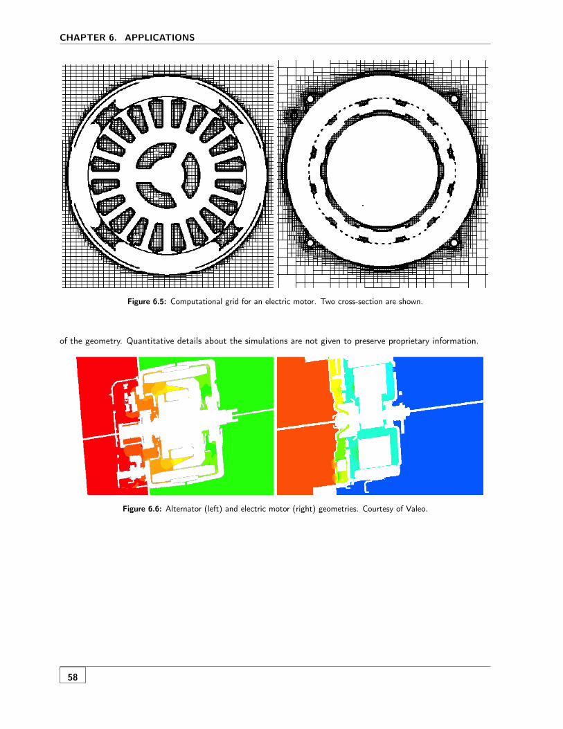
CHAPTER 6. APPLICATIONS

Figure 6.5: Computational grid for an electric motor. Two cross-section are shown.

of the geometry. Quantitative details about the simulations are not given to preserve proprietary information.

Figure 6.6: Alternator (left) and electric motor (right) geometries. Courtesy of Valeo.

58

7Supplementary Material

For an in-depth understanding of the various Immersed Boundary methods and the details of the implementationit is suggested to study the following papers.

1. The review of the main literature on the technique by Mittal and Iaccarino

Immersed Boundary Method Ann. Rev. Fluid Mech. Vol. 37, 239–262, 2005

2. The original paper published by Peskin

Flow Patters around Heart Valves: A Numerical Method JCP Vol. 10, 252-271, 1972

3. The discrete forcing approach by Fadlun et al.

Combined Immersed-Boundary Finite-Difference Methods for Three-Dimensional Complex Flow Sim-ulations JCP Vol. 161, 35-60, 2000

4. The projection approach by Taira and Colonius

The immersed boundary method: A projection approach, JCP, Vol. 225, 2118-2137, 2007

59

Bibliography

[1] Peskin CS. 1972. Flow patterns around heart valves: a digital computer method for solving the equations ofmotion. Ph.D. thesis, Physiology, Albert Einstein College of Medicine. University Microfilms. 378:72-30.

[2] Beyer RP, Leveque RJ. 1992. Analysis of a one-dimensional model for the immersed boundary method. SIAMJ. of Num. Anal. 29:332–364.

[3] Lai MC, Peskin CS. 2000. An immersed boundary method with formal second-order accuracy and reducednumerical viscosity. J. Comput. Phys. 160:705–719.

[4] Iaccarino G, Verzicco R. 2003. Immersed boundary technique for turbulent flow simulations. Appl. Mech. Rev.56:331–347.

[5] Mittal R, Iaccarino, G. 2005. Immersed Boundary Method. Ann. Rev. Fluid Mech. 37:239–262.

[6] Berger MJ, Aftosmis MJ. 1998. Aspects (and aspect ratios) of Cartesian mesh methods. Proc. 16th Interna-tional Conf. on Num. Meth. in Fluid Dynamics.

[7] Mittal R, Bonilla C, Udaykumar HS. 2003. Cartesian grid methods for simulating flows with moving boundaries.in Computational Methods and Experimental Measurements-XI, Ed. Brebbia, Carlomagno & Anagnostopoulous.

[8] Iaccarino G, Kalitzin G, Moin P, Khalighi B. 2004. Local grid refinement for an immersed boundary RANSsolver. AIAA Paper 2004-0586.

[9] Verzicco R, Fatica M, Iaccarino G, Moin P, Khalighi B. 2001. Large eddy simulation of a road-vehicle withdrag reduction devices. AIAA J. 40:2447–2455.

[10] Balaras E. 2004. Modeling Complex Boundaries using an external force field on fixed Cartesian Grids inlarge-eddy simulations. Comput. Fluids 33:375–404.

[11] Zeeuw D, Powell K, 1991. An adaptively-refined Cartesian mesh solver for the Euler equations. AIAA Paper1991-1542.

[12] Wu Z, 1998. Anisotropic Cartesian Grid Method for Viscous Flow Computation. in Computational FluidDynamics Review, Ed. M. Hafez, K. Oshima.

[13] Wang ZJ, Chen RF, Hariharan N, Przekwas AJ, Grove D. A 2n Tree Based Automated Viscous CartesianGrid Methodology for Feature Capturing. AIAA Paper 1999-3300.

[14] Kravchenko AG, Moin P, Moser R. 1996. Zonal embedded Grids for Numerical Simulations of Wall-BoundedTurbulent Flows. J. Comp. Physics 127:412-423.

[15] Seidi, V., Muzaferija, S., Peric, M. Parallel Computation of Unsteady Separated Flows Using Unstructured,Locally Refined Grids. Notes on Numerical Fluid Mechanics. Ed. R. Friedrich and P. Bontoux.

[16] Mahesh, C., Constantinescu, G., Moin, P. 2004. A Numerical Method for Large-Eddy Simulation in ComplexGeometries. J. Comp. Physics 197:215–240.

[17] Ham, F. & Iaccarino, G., 2004. Energy Conservation in Colocated Discretization Schemes on UnstructuredMeshes. Annual Research Briefs, Center for Turbulence Research 3–14.

[18] Kim J, Kim D & Choi H. 2001. An immersed-boundary finite-volume method for simulations of flow incomplex geometries. J. Comput. Phys. 171:132–150.

[19] T. J. Tautges, 2004, "The Common Geometry Module", SANDIA Report SAND2004-6252

[20] R. Haimes, ÒCAPRI: Computational Analysis Programming Interface, A Solid Modeling Based Infra-structurefor Engineering Analysis and DesignÓ, 2000, CAPRI userÕs guide, MIT, Revision 1.00, Dec. 18.

[21] L. Piegl, 1991."On NURBS: A Survey", IEEE Computer Graphics and Applications, Vol. 11, No. 1, pp. 55 -71.

61

BIBLIOGRAPHY

[22] J. O’Rourke, 1988, "Computational Geometry in C", Cambridge University Press.

[23] Edelsbrunner, H., and Mcke, E.P., 1990, "Simulation of Simplicity: A Technique to Cope with DegenerateCases in Geometric Algorithms." ACM Transactions of Graphics, 9(1):66-104.

[24] Behnia, M., Parneix, S., Durbin, P., 1998. Prediction of Heat Transfer in an Axisymmetric TurbulentJet Impinging on a Flat Plate. Int. J. Heat & Mass Transfer, 41, 1845-1855.

[25] Bredberg, J. & Davidson, L., 1999. Prediction of flow and heat transfer in a stationary 2D rib roughenedpassage using low-Re turbulent models. in 3rd European Conference on Turbomachinery, 963-972.

[26] Chyu, M. K., Wu, L. X., 1989. Combined effects of rib angle-of-attack and pitch-to-height ratio on masstransfer from a surface with transverse ribs. Exp. Heat Transfer, 2, 291-308.

[27] Durbin, P. A., 1991. Near-Wall Turbulence Closure Modeling Without “Damping Functions”. Theor. andComp. Fluid Dynamics, 3, 1-13.

[28] Durbin, P. A., 1993. Application of a near-wall turbulence model to boundary layers and heat transfer,Int. J. Heat and Fluid Flow, 14(4), 316-323.

[29] Gatski, T. B., Speziale, C. G., 1993. On explicit algebraic stress models for complex turbulent flows.J. Fluid Mech, 254, 59-78.

[30] Han, J. C., Glicksman, L. R., Rohsenow W. M., 1978. An investigation of heat transfer and frictionfor rib-roughened surfaces. Int. J. Heat Mass Transfer, 21, 1143-1156.

[Han et. al. (1985)] Han, J. C., Park, J. S., Lei, C. K., 1985. Heat Transfer Enhancement in ChannelsWith Turbulence Promoters. J. of Engr. for Gas Turbines and Power, 107, 628-635.

[31] Iacovides, H., Raisee, M. 1999. Recent progress in the computation of flow and heat transfer in internalcooling passages of turbine blades. Int. J. Heat and Fluid Flow, 20, 320-328.

[32] Iaccarino, G., 2001. Prediction of a Turbulent Separated Flow using Commercial CFD Codes. ASME J.of Fluids Eng., 123(4), 1-9.

[33] Launder, B. E., & Spalding, D. B., 1972. Mathematical Models of Turbulence. Academic Press,London.

[34] Liou, T. M., Hwang, J. J., Chen, S. H., 1993. Simulation and measurement of enhanced turbulentheat transfer in a channel with periodic ribs on one principal wall. Int. J. Heat Mass Transfer, 36(2), 507-517.

[35] Ooi, A., Iaccarino, G., Durbin, P. A. & Behnia, M., 2002. Reynolds Averaged Simulation of Flowand Heat Transfer in Ribbed Ducts. submitted to International Journal of Heat and Fluid Flow.

[36] Rau, G., Cakan, M., Moeller, D. Arts, T., 1998. The Effect of Periodic Ribs on the Local Aerody-namic and Heat Transfer Performance of a Straight Cooling Channel. J. Turbomachinery, 120, 368-375.

[37] Ravigururajan, T. S. & Bergles, A. E., 1996. Development and Verification of General Correlationsfor Pressure Drop and Heat Transfer in Single-Phase Turbulent Flow in Enhanced Tubes. Experimental Thermaland Fluid Science, 13(1), 55-71.

[38] Rodi, W., 1991. Experience with two-layer models combining the k − ε model with a one-equation modelnear the wall. AIAA Paper 91-0216.

[39] Simoneau, R. J., Simon, F. F., 1992. Progress towards understanding and predicting heat transfer inthe turbine gas path. Int. J. Heat and Fluid Flow, 14(2), 106-128.

[40] Stephens, M. A., 1995. Computation of Flow and Heat Transfer in a Rectangular Channel with Ribs.AIAA Paper 95-0180.

[41] Launder, B. E., & Sharma, A., 1974. Application of the Energy-Dissipation Model of Turbulence tothe Calculation of Flow Near a Spinning Disk. Letters in Heat and Mass Transfer, 1, 131-138.

62

BIBLIOGRAPHY

[42] Lam C. K. G. & Bremhorst K., 1981. A modified form of the k−ε model for predicting wall turbulence.ASME J. Fluids Engng., 103, 456-462.

[43] Chang, K.C. Hsieh, W.D., & Chen, C.S., 1995. A Modified Low-Reynolds-Number Turbulence ModelApplicable to Recirculating Flow in Pipe Expansion. ASME, J. Fluids Eng., 117(3), 417-423.

[44] Wilcox, D. C. W., 1998. Turbulence Modeling for CFD, DCW Industries.

[45] Anderson DM, McFadden GB, Wheeler AA. 1998. Diffuse-interface methods in fluid mechanics. Annu. Rev.Fluid Mech.. 30:139–165.

[46] Angot P, Bruneau CH, Frabrie P. 1999. A penalization method to take into account obstacles in viscousflows. Numerische Mathematik. 81:497–520.

[47] Balaras E. 2004. Modeling Complex Boundaries using an external force field on fized Cartesian Grids inlarge-eddy simulations. Comput. Fluids 33:375–404.

[48] Baum JD, Luo H, Lonher R. 1998. The numerical simulation of strongly unsteady flows with hundreds ofmoving bodies. AIAA Paper 1998-0788.

[49] Berger MJ, Aftosmis MJ. 1998. Aspects (and aspect ratios) of Cartesian mesh methods. Proc. 16th Inter-national Conf. on Num. Meth. in Fluid Dynamics.

[50] Beyer RP, Leveque RJ. 1992. Analysis of a one-dimensional model for the immersed boundary method. SIAMJ. of Num. Anal. 29:332–364.

[51] Beyer RP. 1992. A computational model of the cochlea using the immersed boundary method. J. Comp.Phys.. 98:145–162.

[52] Brinkman HC. 1947. A calculation of the viscous force exerted by a flowing fluid on a swarm of particles.Appl. Sci. Res. 1:27-34.

[53] Clarke D, Salas M, Hassan H. 1986. Euler calculations for multi-element airfoils using Cartesian grids. AIAAJ. 24:1128-1135.

[54] Constantinescu, G. & Squires, K. 2004 Numerical investigations of flow over a sphere in the subcriticaland supercritical regimes. Phys. Fluids 16, 1449–1466.

[55] Fauci LJ, McDonald A. 1994. Sperm motility in the presence of boundaries. B. Math. Biol. 57:679-692.

[56] Fedkiw R, Liu XD. 2002. The ghost fluid method for viscous flows. Innovative Methods for NumericalSolutions of Partial Differential Equations, ed. M. Hafez, J.J. Chattot, World Scientific Publishing. 111–143.

[57] Ferziger JH, Peric M. 1996. Computational methods in fluid dynamics. Springer-Verlag, New York.

[58] Ghias R, Mittal R, Lund TS. 2004. A non-body conformal grid method for simulation of compressible flowswith complex immersed boundaries. AIAA Paper 2004-0080.

[59] Glowinski R, Pan TW, Periaux J. 1994. A fictitious domain method for external incompressible viscous flowsmodeled by Navier-Stokes equations. Comput. Meth. Appl. Mech. Eng. 112:133–148.

[60] Goldstein D, Handler R, Sirovich L. 1993. Modeling a no-slip flow boundary with an external force field. J.Comput. Phys. 105:354–366.

[61] Iaccarino G, Verzicco R. 2003. Immersed boundary technique for turbulent flow simulations. Appl. Mech.Rev. 56:331–347.

[62] Iaccarino G, Kalitzin G, Elkins C. 2003. Numerical and experimental investigation of the turbulent flow inribbed serpentine passage. Annual Research Brief, Center for Turbulence Research. 379–388.

[63] Iaccarino G, Kalitzin G, Moin P, Khalighi B. 2004. Local grid refinement for an immersed boundary RANSsolver. AIAA Paper 2004-0586.

63

BIBLIOGRAPHY

[64] Kalitzin G, Iaccarino G, Khalighi B. 2003. Towards and immersed boundary solver for RANS simulations.AIAA Paper 2003-0770.

[65] Khadra K, Angot P, Parneix S, Caltagirone JP. 2000. Fictitious domain approach for numerical modeling ofNavier-Stokes equations. Int. J. Num. Meth. Fluids. 34:651–684.

[66] Kim, H. J. & Durbin, P. A. 1988 Observations of the frequencies in a sphere wake and of drag increaseby acoustic excitation. Phys. Fluids 31, 3260–3265.

[67] Kim, J., Kim, D. & Choi, H. 2001 An immersed-boundary finite-volume method for simulations of flowin complex geometries. J. Comput. Phys. 171, 132–150.

[68] Lai MC, Peskin CS. 2000. An immersed boundary method with formal second-order accuracy and reducednumerical viscosity. J. Comput. Phys. 160:705–719.

[69] Leveque RJ, Li Z. 1994. The immersed interface method for elliptic equations with discontinuous coefficientsand singular sources. SIAM J. Num. Anal. 31:1001–1025.

[70] Majumdar S, Iaccarino G, Durbin PA. 2001. RANS solver with adaptive structured boundary non-conforminggrids. Annual Research Briefs 2001, Center For Turbulence Research. 353–364.

[71] Mittal R, Seshadri V, Sarma S, Udaykumar HS. 2002a. Computational modeling of fluidic micro-handlingprocesses. in Tech. Proc. Fifth Int Conf. Modeling and Simulation of Microsystems, San Juan, Puerto-Rico,388-391.

[72] Mittal R, Utturkar Y, Udaykumar HS. 2002b. Computational modeling and analysis of biomimetic flightmechanisms. AIAA Paper 2002-0865.

[73] Mittal R, Seshadri V, Udaykumar HS. 2004. Flutter, tumble and vortex induced autorotation. To appear inTheor. Comput. Fluid Dyn.

[74] Mittal R, Bonilla C, Udaykumar HS. 2003. Cartesian grid methods for simulating flows with moving bound-aries. in Computational Methods and Experimental Measurements-XI, Ed. Brebbia, Carlomagno & Anagnos-topoulous.

[75] Mittal R, Najjar FM, Byrganhalli R, Seshadri V, Singh H. (2004) Simulation of complex biological flows andflow control problems on Cartesian grids. To Appear Proc. Fifth Int. Conf. on Advances in Fluid Mechanics.

[76] Mohd-Yosuf J. 1997. Combined immersed boundary/B-spline methods for simulation of flow in complexgeometries. Annual Research Briefs, Center for Turbulence Research. 317–328.

[77] Patankar NA. 2001. A formulation for fast computation of rigid particulate flows. Annual Research Brief,Center for Turbulence Research. 197–208.

[78] Peskin CS. 1972. Flow patterns around heart valves: a digital computer method for solving the equations ofmotion. Ph.D. thesis, Physiology, Albert Einstein College of Medicine. University Microfilms. 378:72-30.

[79] Peskin CS. 1981. The fluid dynamics of heart valves: experimental, theoretical and computational methods.Annu. Rev. Fluid Mech. 14:235-259.

[80] Quarteroni A, Valli A. 1999. Domain decomposition methods for partial differential equations. Oxford Uni-versity Press.

[81] Ramamurti R, Sandberg WC. 2001. Simulation of flow about flapping airfoils using a finite element incom-pressible flow solver. AIAA J. 39:253-352.

[82] Roma AM, Peskin CS, Berger MJ. 1999. An Adaptive version of the immersed boundary method. J. Comput.Phys. 153:509-534.

[83] Sakamoto, H. & Haniu, H. 1990 A study on vortex shedding from spheres in a uniform flow.Trans. ASME: J. Fluids Eng. 112, 386–392.

64

BIBLIOGRAPHY

[84] Saiki EM, Biringen S. 1996. Numerical simulation of a cylinder in uniform flow: application of a virtualboundary method. J. Comput. Phys. 123:450-465.

[85] Scardovelli R, Zaleski S. 1999. Direct numerical simulation of free-surface and interfacial flows. Annu. Rev.Fluid. Mech. 31:567-603.

[86] Schlichting H, Gersten K. 1996. Boundary layer theory. Springer-Verlag.

[87] Stockie JM, Wetton BR. 1998. Analysis of stiffness in the immersed boundary method and implications fortime-stepping schemes. J. Comput. Phys. 154:41–64.

[88] Tezduyar TE. 2001. Finite element methods for flow problems with moving boundaries and interfaces. Arch.Comput. Meth. Engr.. 8:83-130.

[89] Tran L, Udaykumar HS. 2004. A particle-levelset based sharp interface Cartesian grid method for impact,penetration and void collapse. J. Comp. Phys. 193:469-510.

[90] Udaykumar HS, Shyy W, Rao MM. 1996. Elafint: A mixed Eulerian-Lagrangian method for fluid flows withcomplex and moving boundaries. Int. J. Numer. Meth. Fluids. 22:691–705.

[91] Udaykumar HS, Mittal R, Rampunggoon P, Khanna A. 2001. A sharp interface Cartesian grid method forsimulating flows with complex moving boundaries. J. Comput. Phys. 174:345-380.

[92] Udaykumar HS, Mittal R, Shyy W. 1999. Computation of solid-liquid phase fronts in the sharp interface limiton fixed grids. J. Comput. Phys. 153:534-574.

[93] Udaykumar HS, Mittal R, Rampunggoon P. 2002. Interface tracking finite volume method for complex solid-fluid interactions on fixed meshes. Comm. Numer. Meth. Engr. 18:89-97.

[94] Unverdi S, Tryggvason G. 1992. A front-tracking method for viscous, incompressible, multifluid flows. J.Comput. Phys. 100:25–42.

[95] Utturkar Y, Mittal R. 2002. Sensitivity of synthetic jets to the design of the jet cavity. AIAA Paper 2002-0124.

[96] Werlé, H. 1980 ONERA photograph in An Album of Fluid Motion assembled by M. Van Dyke (page 34).The Parabolic Press, Stanford, California.

[97] Verzicco R, Mohd–Yusof J, Orlandi P, Haworth D. 2000. LES in complex geometries using boundary bodyforces. AIAA J. 38:427–433.

[98] Verzicco R, Fatica M, Iaccarino G, Moin P, Khalighi B. 2001. Large eddy simulation of a road-vehicle withdrag reduction devices. AIAA J. 40:2447–2455.

[Ye et al.(1999)] Ye T, Mittal R, Udaykumar HS, Shyy W. 1999. An accurate Cartesian grid method for viscousincompressible flows with complex immersed boundaries. J. Comput. Phys. 156:209-240.

[Yun, Choi & Kim(2003)] Yun, G., Choi, H. & Kim, D. 2003 Turbulent flow past a sphere at Re = 3700and 104. Phys. Fluids 15, S6.

[99] Zeeuw D, Powell K, 1991. An adaptively-refined Cartesian mesh solver for the Euler equations. AIAA Paper1991-1542.

[100] Zhang J, Childress S, Libchaber A, Shelley M. 2000. Flexible filaments in a flowing soap film as a modelfor one-dimensional flags in a two-dimensional wind. Nature. 408:835-845.

[101] Zhu L, Peskin C. 2003. Interaction of two filaments in a flowing soap film. Phys. Fluids 15:128–136.

65

Documents

The Immersed Boundary Method - monsite-1 · Turbine blades are exposed to ... case the thermal load is generated ... The primary advantage of the immersed boundary method is associated