Embed Size (px)
Citation preview
The Ideal Monatomic Gas
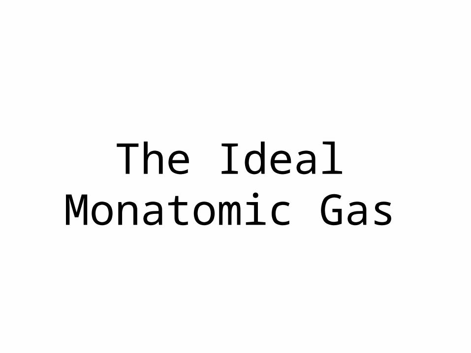
Canonical ensemble: N, V, T
2
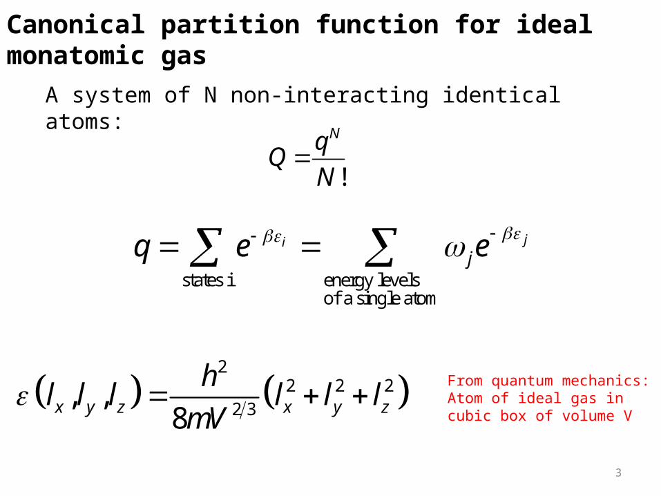
Canonical partition function for ideal monatomic gas
A system of N non-interacting identical atoms:
!
NqQ
N
states i energy levelsof a single atom
jijq e e
2
2 2 22 3
, ,8x y z x y z
hl l l l l l
mV
From quantum mechanics:Atom of ideal gas in cubic box of volume V
3
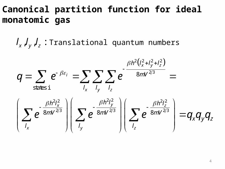
Canonical partition function for ideal monatomic gas
Translational quantum numbers, , :x y zl l l
2 2 2 2
2 3
2 22 2 2 2
2 3 2 3 2 3
8
states i
8 8 8
x y z
i
x y z
yx z
x y z
h l l l
mV
l l l
h lh l h l
mV mV mVx y z
l l l
q e e
e e e q q q
4
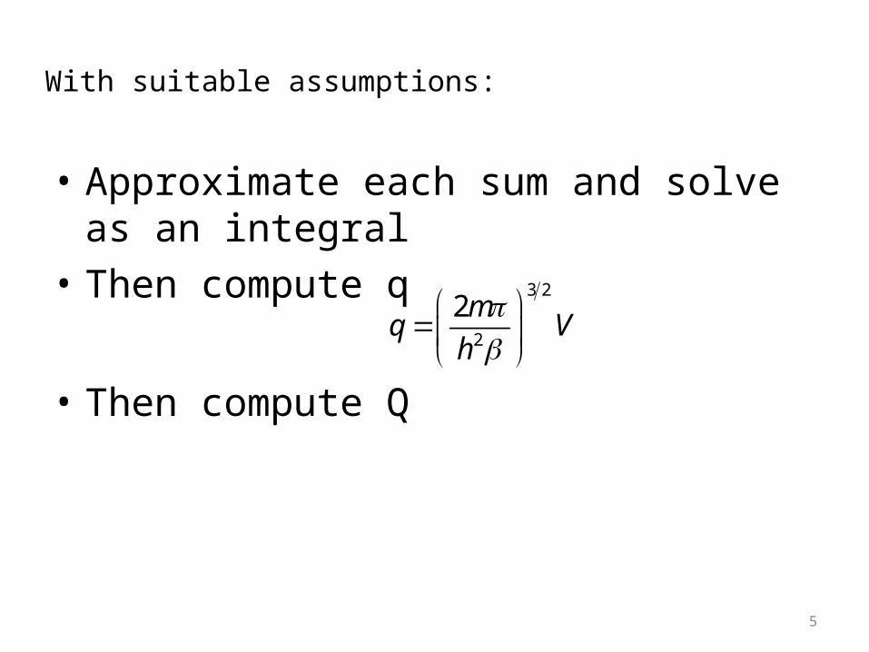
With suitable assumptions:
3 2
2
2mq V
h
• Approximate each sum and solve as an integral
• Then compute q
• Then compute Q
5
The calculated Q is the canonical partition function for ideal monatomic gas
We have considered the contribution of atomic translation to the partition function
However, we have not included other effects, such as contribution of the electronic and nuclear energy states.
We will get back to this matter later in this slide set.
6
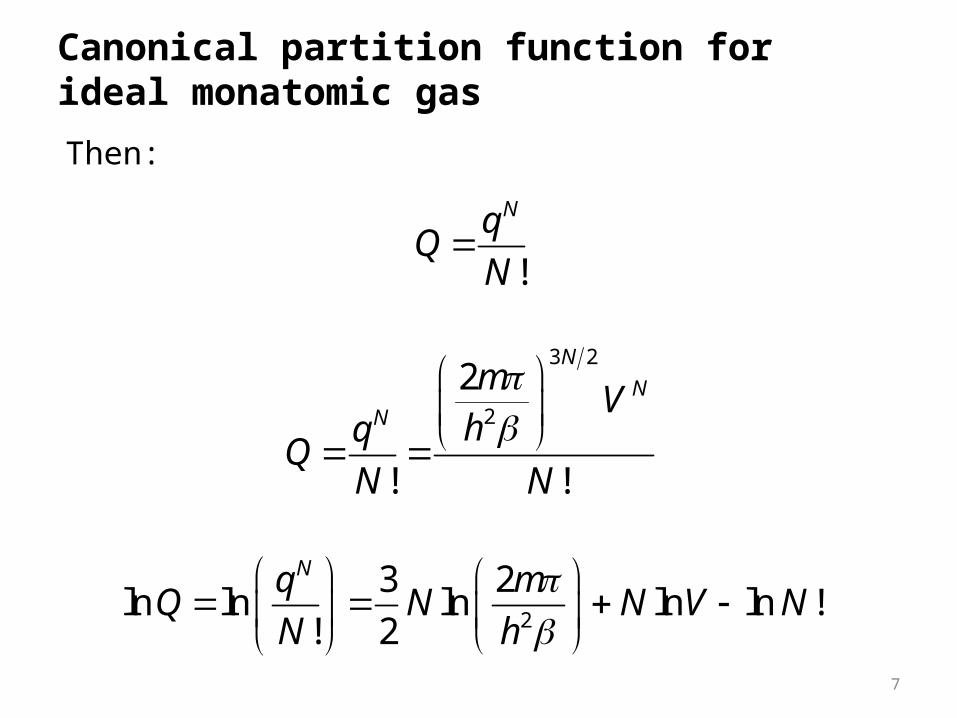
Canonical partition function for ideal monatomic gas
Then:
!
NqQ
N
3 2
2
2
! !
N
NN
mV
hqQ
N N
2
3 2ln ln ln ln ln !
! 2
Nq mQ N N V N
N h
7
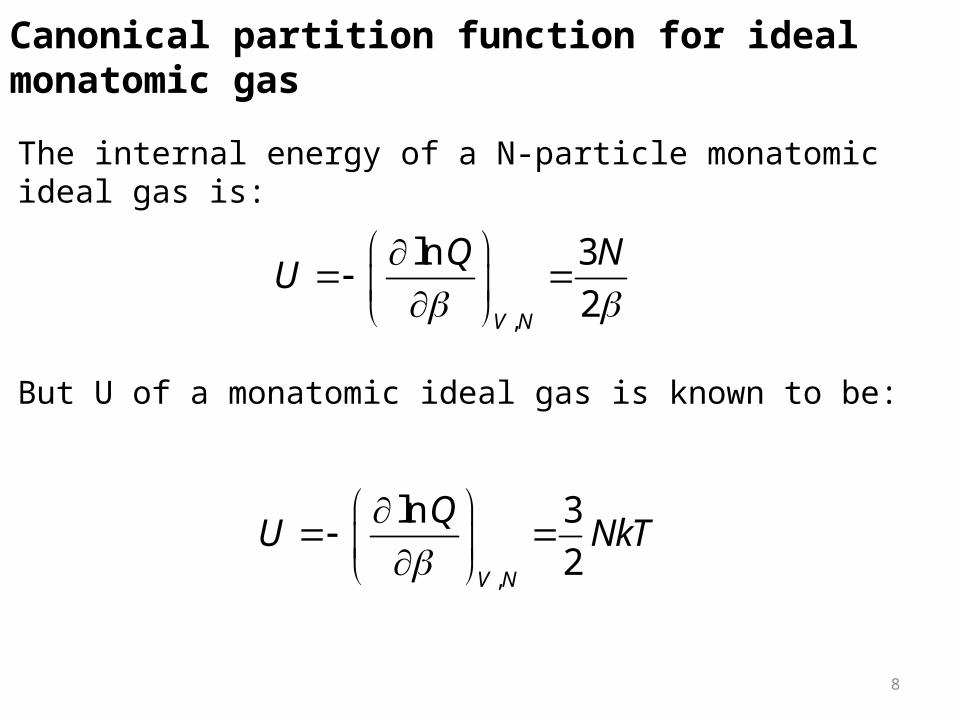
Canonical partition function for ideal monatomic gas
The internal energy of a N-particle monatomic ideal gas is:
,
ln 3
2V N
Q NU
But U of a monatomic ideal gas is known to be:
,
ln 3
2V N
QU NkT
8
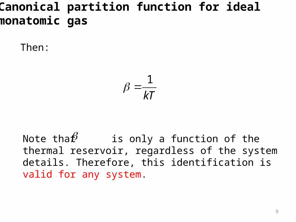
Canonical partition function for ideal monatomic gas
Then:
1
kT
Note that is only a function of the thermal reservoir, regardless of the system details. Therefore, this identification is valid for any system.
9
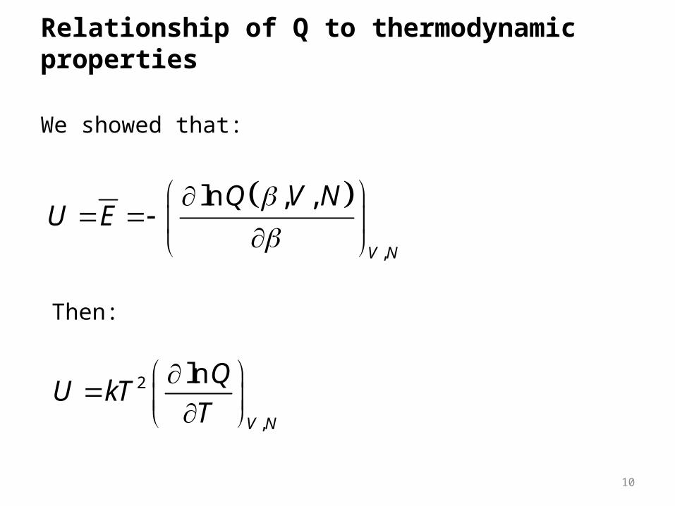
Relationship of Q to thermodynamic properties
Then:
We showed that:
,
ln , ,
V N
Q V NU E
2
,
ln
V N
QU kT
T
10
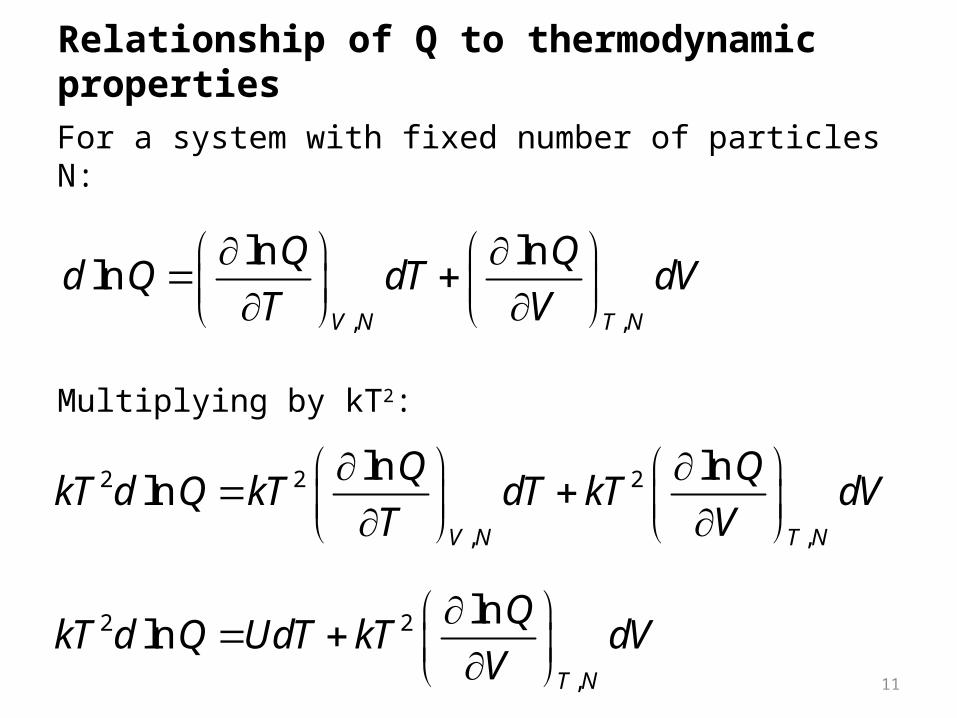
Relationship of Q to thermodynamic properties
Multiplying by kT2:
For a system with fixed number of particles N:
, ,
ln lnln
V N T N
Q Qd Q dT dV
T V
2 2 2
, ,
ln lnln
V N T N
Q QkT d Q kT dT kT dV
T V
2 2
,
lnln
T N
QkT d Q UdT kT dV
V
11
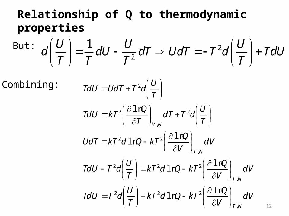
Relationship of Q to thermodynamic properties
Combining:
But: 22
1U U Ud dU dT UdT T d TdU
T T T T
dVV
QkTQdkT
T
UdTTdU
dVV
QkTQdkT
T
UdTTdU
dVV
QkTQdkTUdT
T
UdTdT
T
QkTTdU
T
UdTUdTTdU
NT
NT
NT
NV
,
222
,
222
,
22
2
,
2
2
lnln
lnln
lnln
ln
12
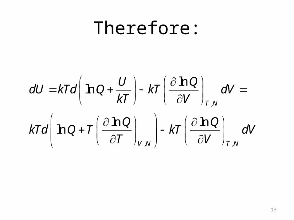
Therefore:
,
, ,
lnln
ln lnln
T N
V N T N
U QdU kTd Q kT dV
kT V
Q QkTd Q T kT dV
T V
13
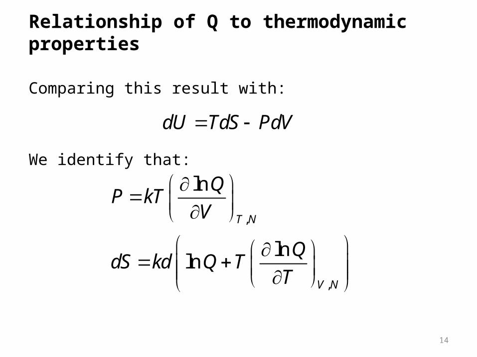
Relationship of Q to thermodynamic properties
We identify that:
Comparing this result with:
dU TdS PdV
,
,
ln
lnln
T N
V N
QP kT
V
QdS kd Q T
T
14
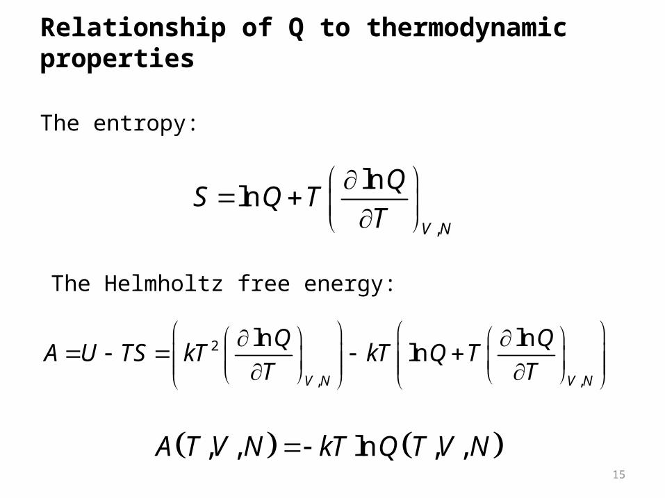
Relationship of Q to thermodynamic properties
The entropy:
,
lnln
V N
QS Q T
T
The Helmholtz free energy:
, , ln , ,A T V N kT Q T V N
2
, ,
ln lnln
V N V N
Q QA U TS kT kT Q T
T T
15
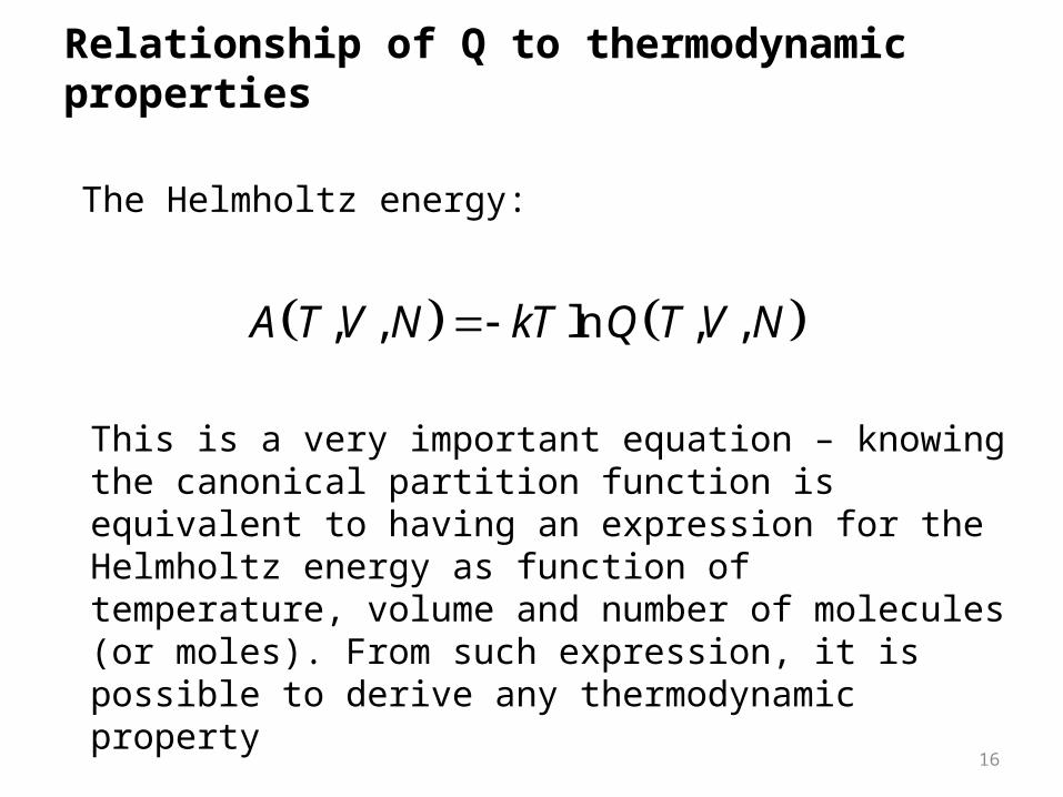
Relationship of Q to thermodynamic properties
The Helmholtz energy:
, , ln , ,A T V N kT Q T V N
This is a very important equation – knowing the canonical partition function is equivalent to having an expression for the Helmholtz energy as function of temperature, volume and number of molecules (or moles). From such expression, it is possible to derive any thermodynamic property
16
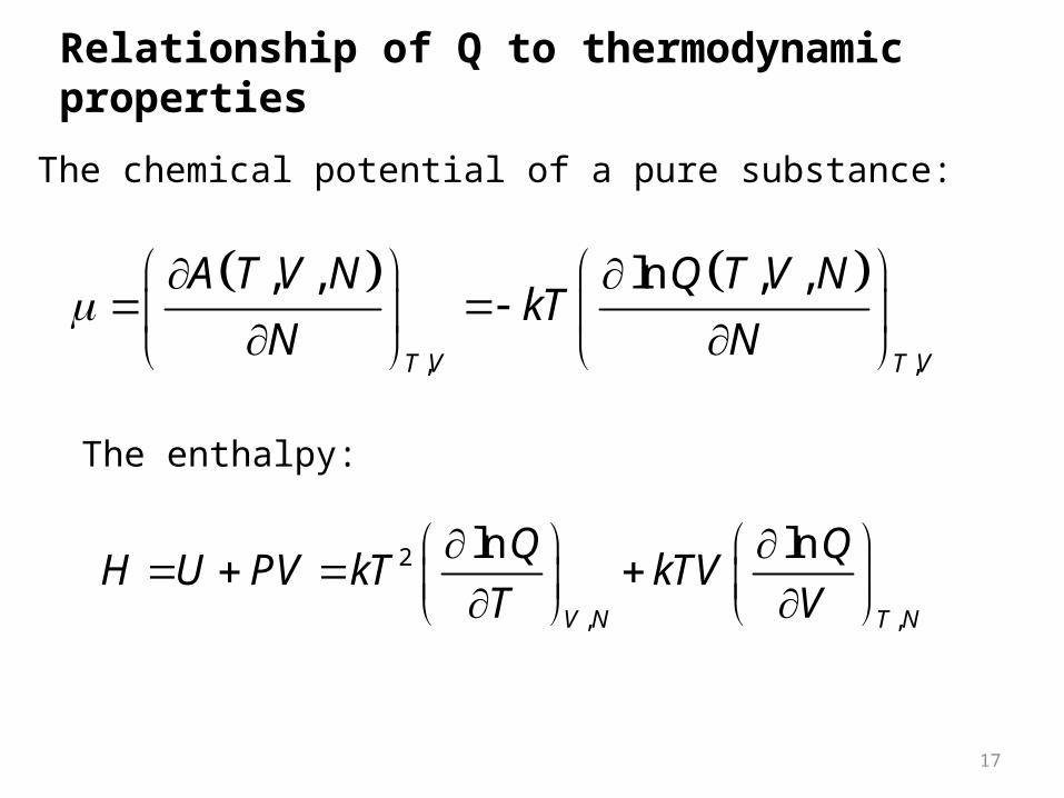
Relationship of Q to thermodynamic properties
The chemical potential of a pure substance:
The enthalpy:
, ,
, , ln , ,
T V T V
A T V N Q T V NkT
N N
2
, ,
ln ln
V N T N
Q QH U PV kT kTV
T V
17
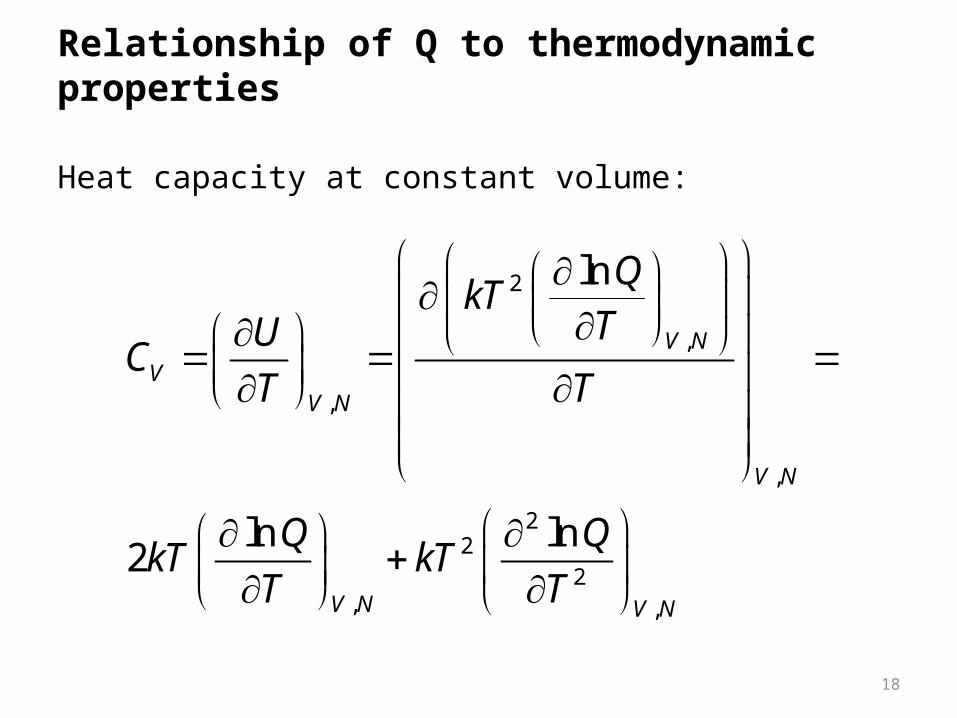
Relationship of Q to thermodynamic properties
Heat capacity at constant volume:
2
,
,
,
22
2, ,
ln
ln ln2
V N
VV N
V N
V N V N
QkT
TUC
T T
Q QkT kT
T T
18
Relationship of Q to thermodynamic properties
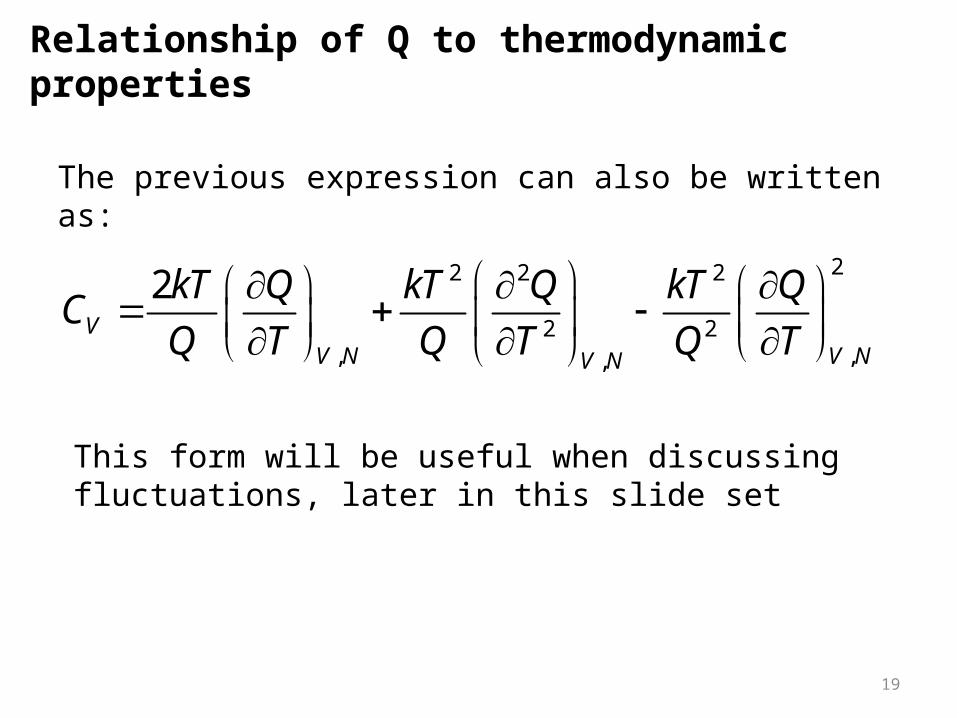
The previous expression can also be written as:
22 2 2
2 2, ,,
2V
V N V NV N
kT Q kT Q kT QC
Q T Q T Q T
This form will be useful when discussing fluctuations, later in this slide set
19
Thermodynamic properties of monatomic ideal gasesThe previous slides showed how to evaluate thermodynamic properties given Q
It is time to discuss the effect of the electronic and nuclear energy states to the single atom partition function before proceeding with additional derivations
We will assume the Born-Oppenheimer approximation: translational energy states are independent of the electronic and nuclear states
Besides, we will assume the electronic and nuclear states are independent of each other
20
Thermodynamic properties of monatomic ideal gases
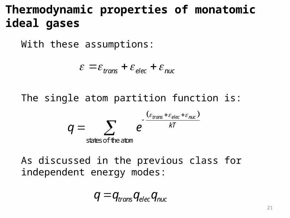
With these assumptions:
trans elec nuc
The single atom partition function is:
states of the atom
trans elec nuc
kTq e
As discussed in the previous class for independent energy modes:
trans elec nucq q q q21

Thermodynamic properties of monoatomic ideal gases
In which:
,
translational states i
trans i
kTtransq e
,
electronic states i
elec i
kTelecq e
,
nuclear states i
nuc i
kTnucq e
22
Thermodynamic properties of monatomic ideal gases
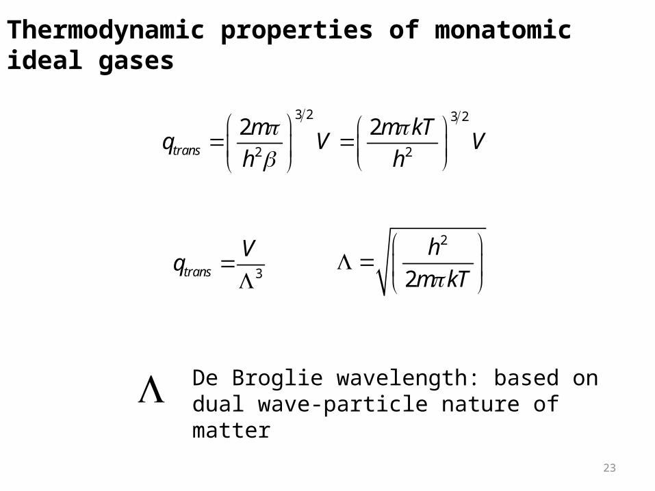
3 2 3 2
2 2
2 2trans
m m kTq V V
h h
3trans
Vq
2
2
h
m kT
De Broglie wavelength: based on dual wave-particle nature of matter
23
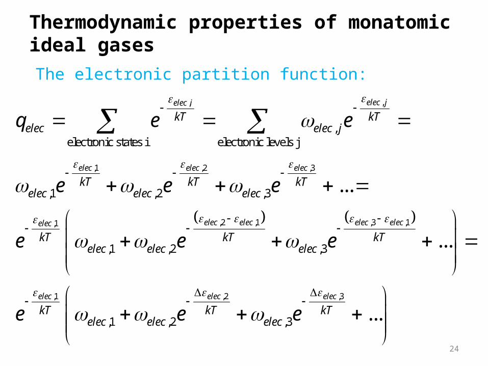
Thermodynamic properties of monatomic ideal gases
The electronic partition function:
,,
,1 ,2 ,3
,2 ,1 ,3,1
,electronic states i electronic levels j
,1 ,2 ,3
,1 ,2 ,3
...
elec jelec i
elec elec elec
elec elec elecelec
kT kTelec elec j
kT kT kTelec elec elec
kT kTelec elec elec
q e e
e e e
e e e
,1
,1 ,2 ,3
,1 ,2 ,3
...
...
elec
elec elec elec
kT
kT kT kTelec elec elece e e
24
Thermodynamic properties of monatomic ideal gases
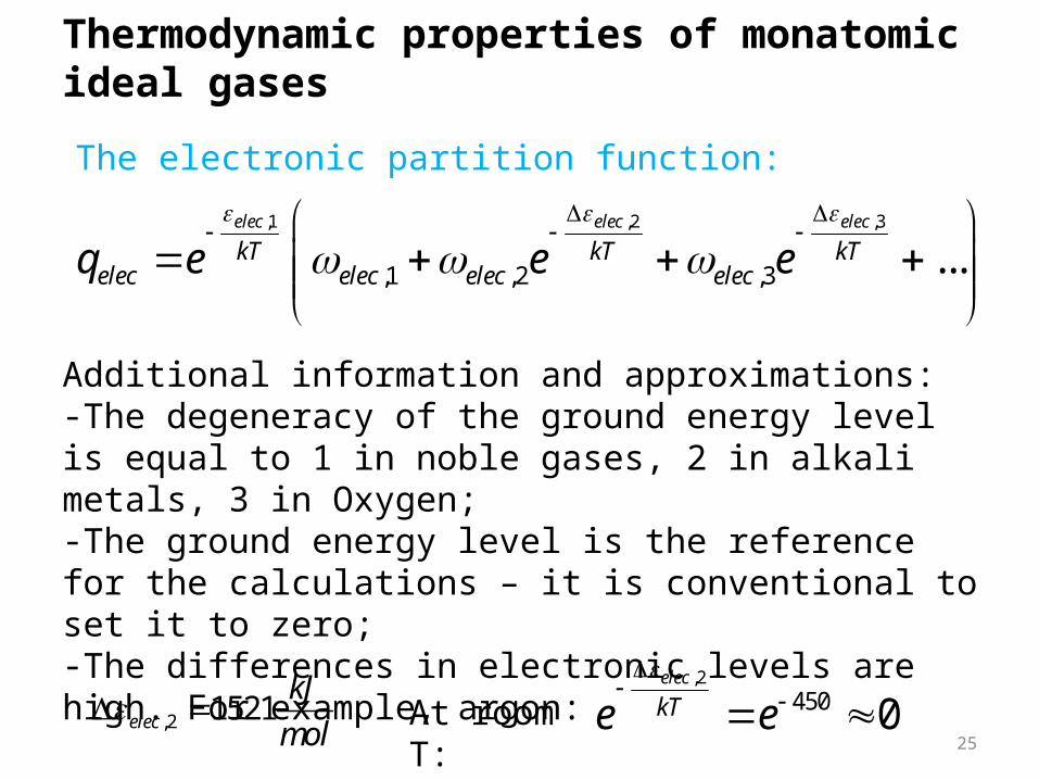
The electronic partition function:
,1 ,2 ,3
,1 ,2 ,3 ...elec elec elec
kT kT kTelec elec elec elecq e e e
Additional information and approximations:-The degeneracy of the ground energy level is equal to 1 in noble gases, 2 in alkali metals, 3 in Oxygen;-The ground energy level is the reference for the calculations – it is conventional to set it to zero;-The differences in electronic levels are high. For example, argon:
,2 1521elec
kJ
mol At room
T:
,2
450 0elec
kTe e
25
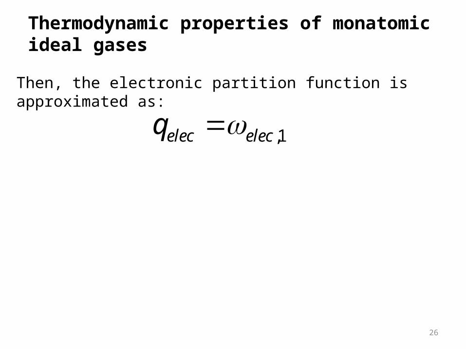
Thermodynamic properties of monatomic ideal gases
Then, the electronic partition function is approximated as:
,1elec elecq
26
Thermodynamic properties of monatomic ideal gases
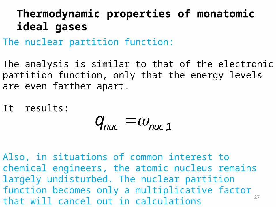
The nuclear partition function:
The analysis is similar to that of the electronic partition function, only that the energy levels are even farther apart.
It results:
,1nuc nucq
Also, in situations of common interest to chemical engineers, the atomic nucleus remains largely undisturbed. The nuclear partition function becomes only a multiplicative factor that will cancel out in calculations 27
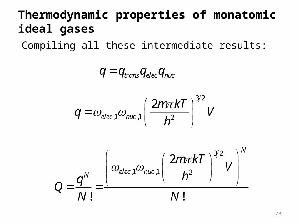
Thermodynamic properties of monatomic ideal gasesCompiling all these intermediate results:
trans elec nucq q q q
3 2
,1 ,1 2
2elec nuc
m kTq V
h
3 2
,1 ,1 2
2
! !
N
elec nucN
m kTV
hqQ
N N
28
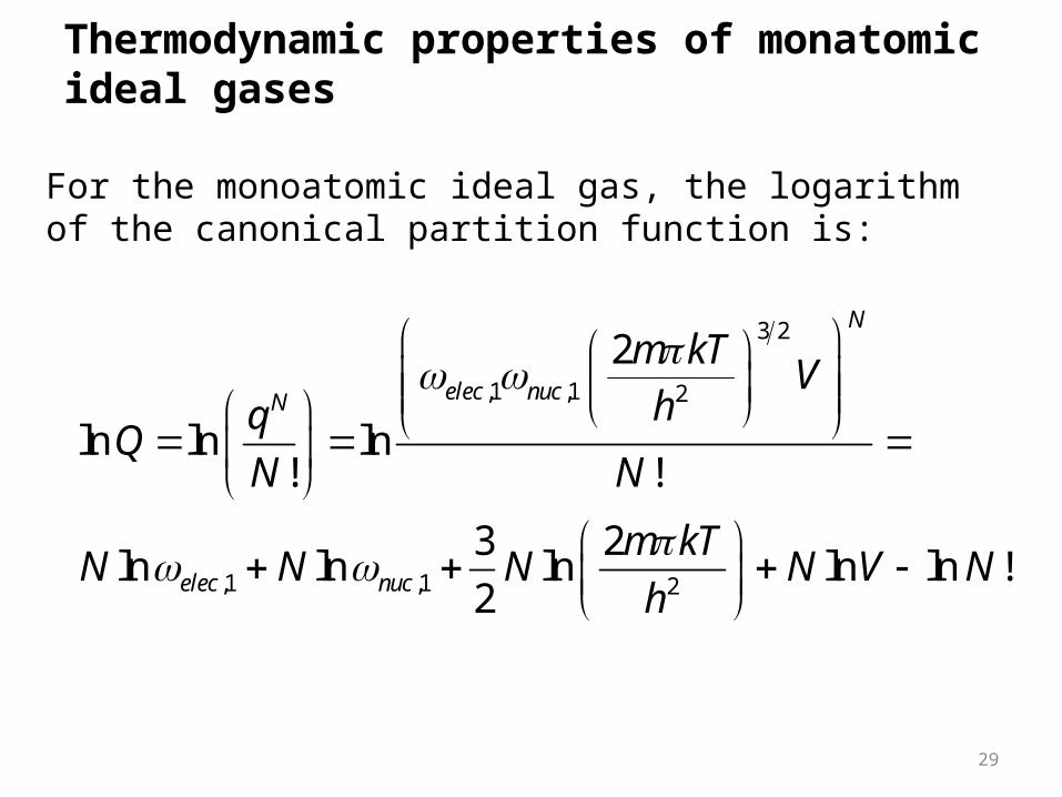
Thermodynamic properties of monatomic ideal gases
For the monoatomic ideal gas, the logarithm of the canonical partition function is:
3 2
,1 ,1 2
,1 ,1 2
2
ln ln ln! !
3 2ln ln ln ln ln !
2
N
elec nucN
elec nuc
m kTV
hqQ
N N
m kTN N N N V N
h
29
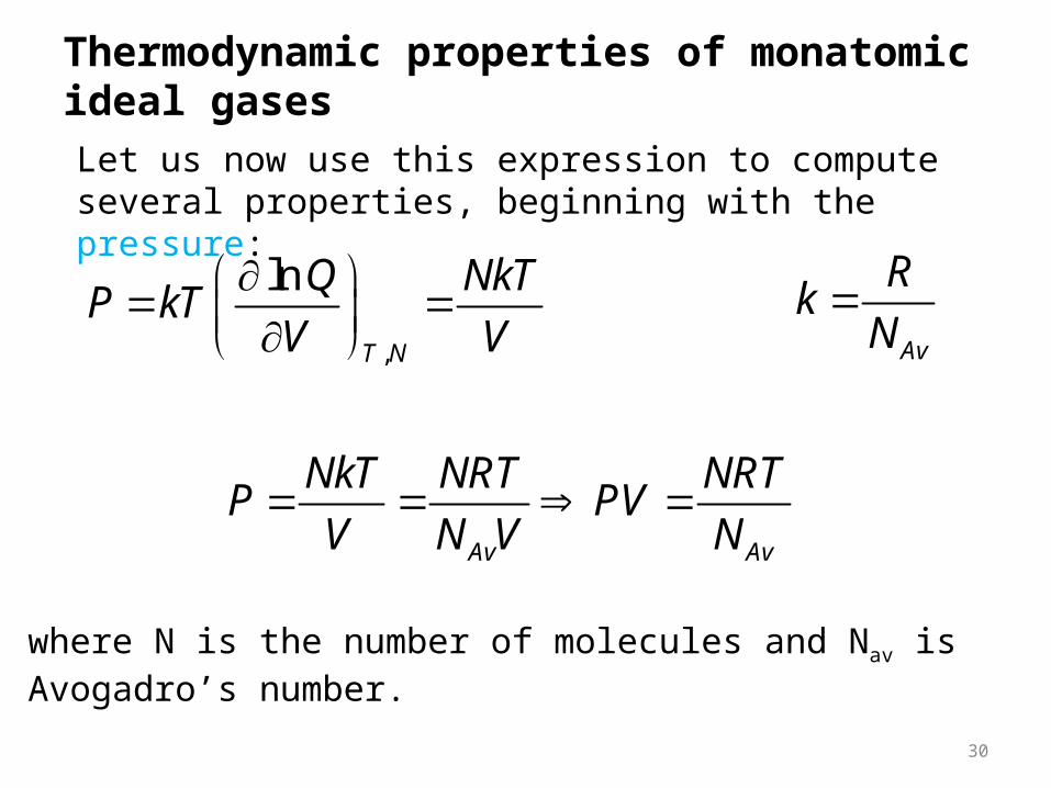
Thermodynamic properties of monatomic ideal gasesLet us now use this expression to compute several properties, beginning with the pressure:
,
ln
T N
Q NkTP kT
V V
Av
Rk
N
Av Av
NkT NRT NRTP PV
V N V N
where N is the number of molecules and Nav is Avogadro’s number.
30
Thermodynamic properties of monatomic ideal gases
PV nRT
31
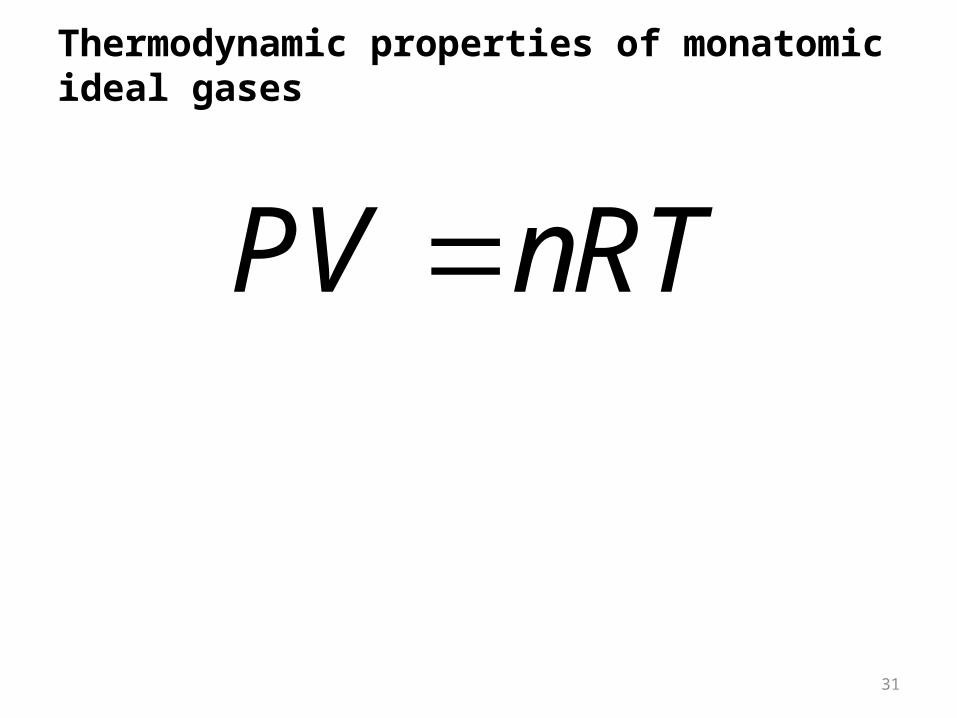
Thermodynamic properties of monatomic ideal gases
PV nRTWe derived this very famous equation from very fundamental principles – an amazing result
32
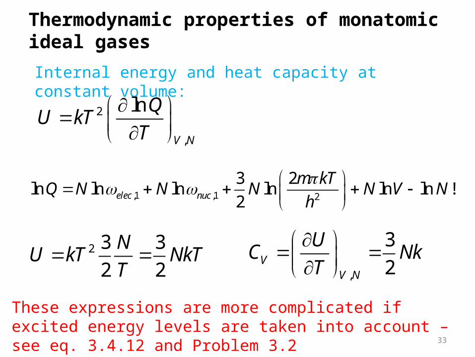
Thermodynamic properties of monatomic ideal gases
Internal energy and heat capacity at constant volume:
2
,
ln
V N
QU kT
T
,1 ,1 2
3 2ln ln ln ln ln ln !
2elec nuc
m kTQ N N N N V N
h
2 3 3
2 2
NU kT NkT
T
,
3
2VV N
UC Nk
T
These expressions are more complicated if excited energy levels are taken into account – see eq. 3.4.12 and Problem 3.2 33
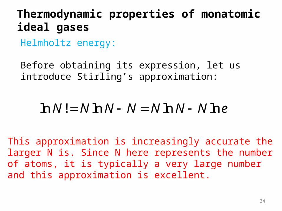
Thermodynamic properties of monatomic ideal gasesHelmholtz energy:
Before obtaining its expression, let us introduce Stirling’s approximation:
ln ! ln ln lnN N N N N N N e
This approximation is increasingly accurate the larger N is. Since N here represents the number of atoms, it is typically a very large number and this approximation is excellent.
34
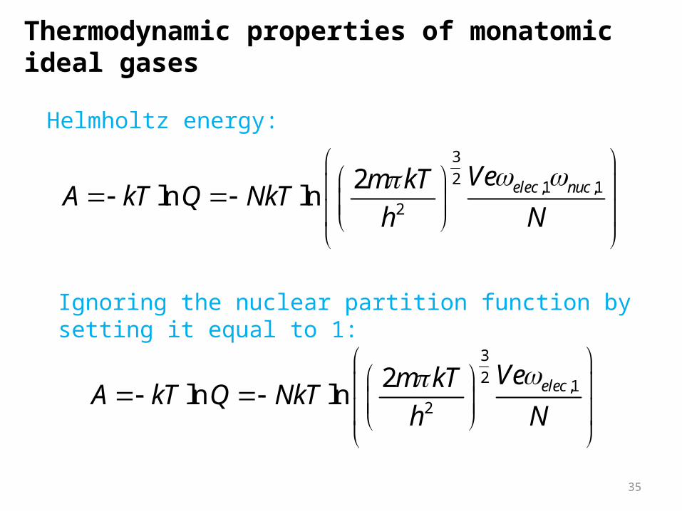
Thermodynamic properties of monatomic ideal gases
Helmholtz energy:
3
2 ,1 ,1
2
2ln ln elec nucVem kT
A kT Q NkTh N
Ignoring the nuclear partition function by setting it equal to 1:
3
2 ,1
2
2ln ln elecVem kT
A kT Q NkTh N
35
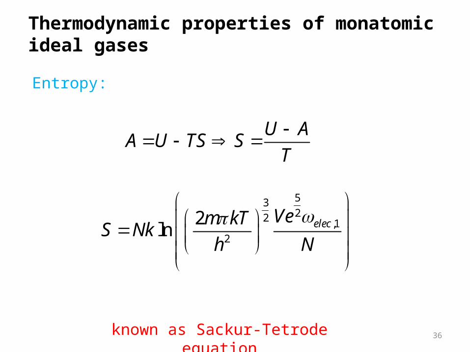
Thermodynamic properties of monatomic ideal gases
Entropy:
U AA U TS S
T
5322 ,1
2
2ln elecVem kT
S Nkh N
known as Sackur-Tetrode equation 36
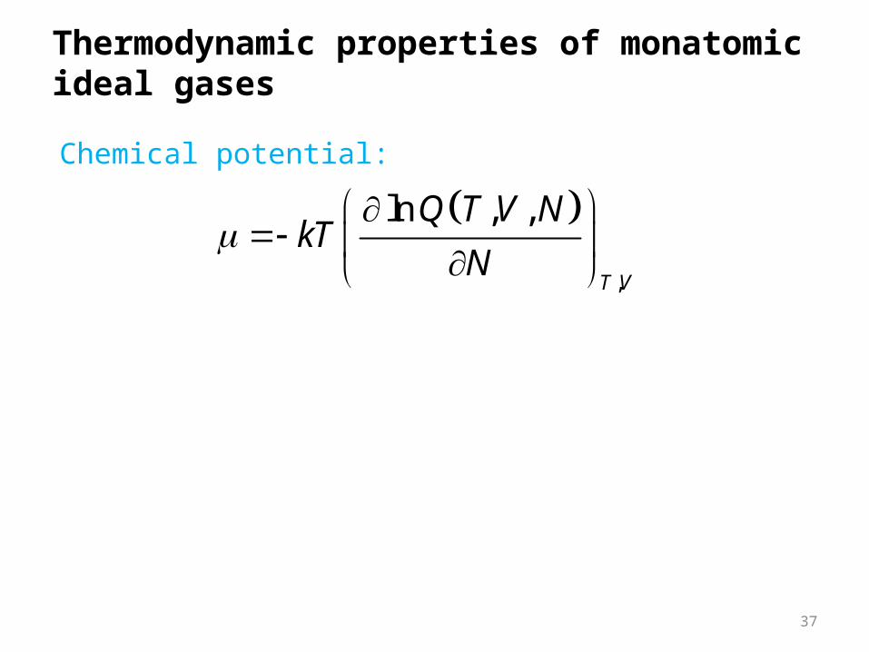
Thermodynamic properties of monatomic ideal gases
Chemical potential:
,
ln , ,
T V
Q T V NkT
N
37
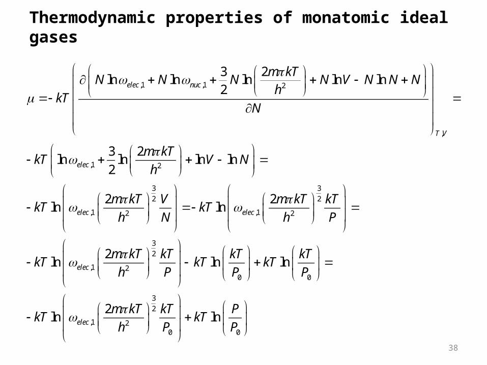
Thermodynamic properties of monatomic ideal gases
,1 ,1 2
,
,1 2
3 3
2 2
,1 ,12 2
3 2ln ln ln ln ln
2
3 2ln ln ln ln
2
2 2ln ln
elec nuc
T V
elec
elec elec
m kTN N N N V N N N
hkT
N
m kTkT V N
h
m kT V m kT kTkT kT
h N h P
3
2
,1 20 0
3
2
,1 20 0
2ln ln ln
2ln ln
elec
elec
m kT kT kT kTkT kT kT
h P P P
m kT kT PkT kT
h P P
38
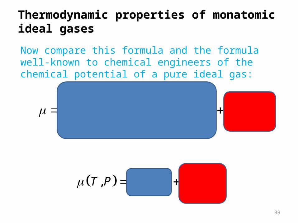
Thermodynamic properties of monatomic ideal gases
Now compare this formula and the formula well-known to chemical engineers of the chemical potential of a pure ideal gas:
00
, , lnP
T P T P kTP
3
2
,1 20 0
2ln lnelec
m kT kT PkT kT
h P P
39
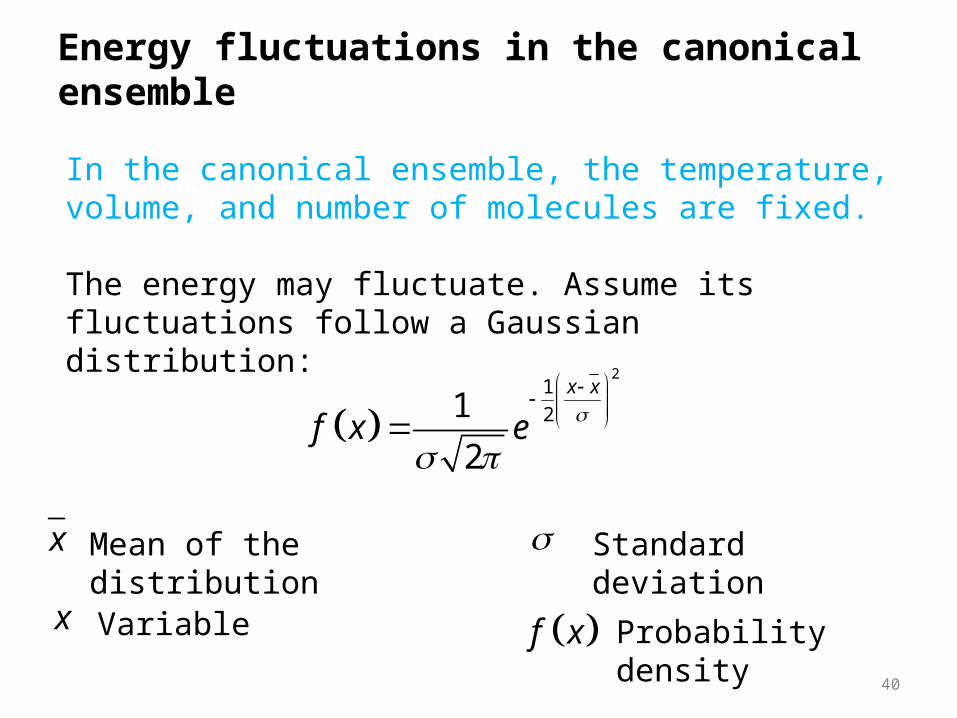
Energy fluctuations in the canonical ensemble
In the canonical ensemble, the temperature, volume, and number of molecules are fixed.
The energy may fluctuate. Assume its fluctuations follow a Gaussian distribution:
2
1
21
2
x x
f x e
x Mean of the distribution Standard deviation
x f xVariable Probability density
40
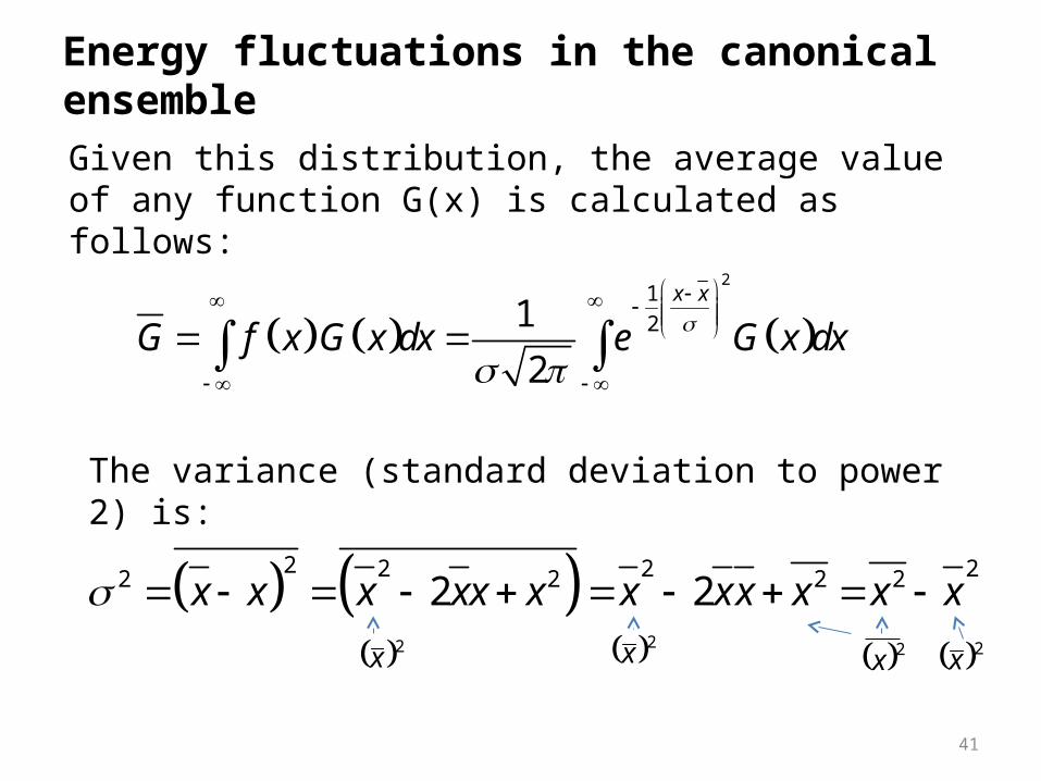
Energy fluctuations in the canonical ensembleGiven this distribution, the average value of any function G(x) is calculated as follows:
2
1
21
2
x x
G f x G x dx e G x dx
The variance (standard deviation to power 2) is:
41
2 2 2 22 2 2 22 2x x x xx x x xx x x x 2x 2x 2x 2x
Energy fluctuations in the canonical ensemble
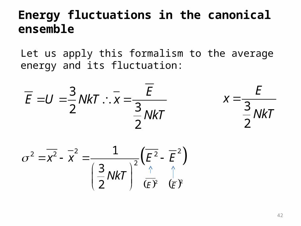
Let us apply this formalism to the average energy and its fluctuation:
3322
EE U NkT x
NkT
32
Ex
NkT
2 22 2 22
1
32
x x E E
NkT
42
2E 2E
Energy fluctuations in the canonical ensemble
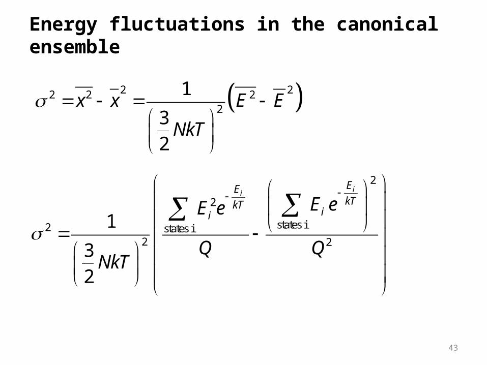
2 22 2 22
1
32
x x E E
NkT
2
2
states i2 states i2 2
1
32
iiEEkTkT
iiE eE e
Q QNkT
43
44
NVNV
j
kTEj
j
kTEj
NVNVNVNV
NVNVNV
NVNV
j
kTEj
NVNV
j
kTEj
NVNV
j
kTEj
j
kTE
T
Q
Q
kT
T
QkT
Q
kT
Q
eE
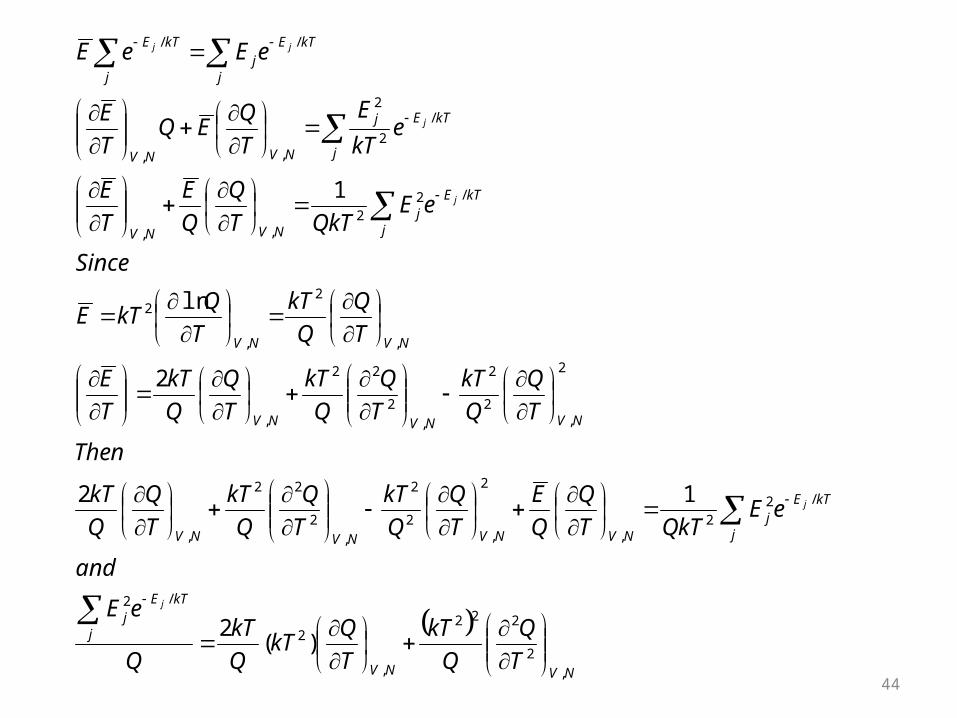
and
eEQkTT
Q
Q
E
T
Q
Q
kT
T
Q
Q
kT
T
Q
Q
kT
Then
T
Q
Q
kT
T
Q
Q
kT
T
Q
Q
kT
T
E
T
Q
Q
kT
T
QkTE
Since
eEQkTT
Q
Q
E
T
E
ekT
E
T
QEQ
T
E
eEeE
j
j
j
j
jj
,
2
222
,
2
/2
/22
,
2
,2
2
,
2
22
,
2
,2
2
,
2
22
,
,
2
,
2
/22
,,
/
2
2
,,
//
)(2
12
2
ln
1
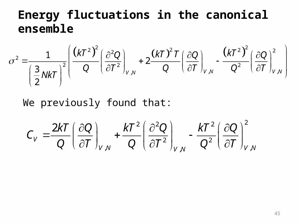
Energy fluctuations in the canonical ensemble
2 222 2 222
2 2 2, ,,
12
32
V N V NV N
kT kTkT TQ Q Q
Q T Q T Q TNkT
22 2 2
2 2, ,,
2V
V N V NV N
kT Q kT Q kT QC
Q T Q T Q T
We previously found that:
45
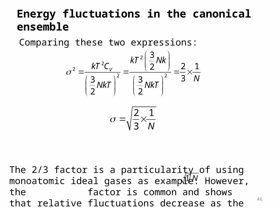
Energy fluctuations in the canonical ensemble
The 2/3 factor is a particularity of using monoatomic ideal gases as example. However, the factor is common and shows that relative fluctuations decrease as the number of molecules increases.
Comparing these two expressions:
22
22 2
32 1233 3
2 2
V
kT NkkT C
NNkT NkT
2 1
3 N
1 N
46
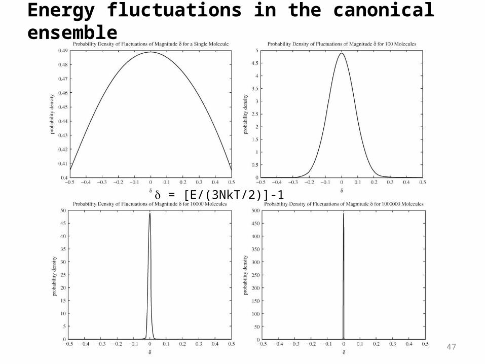
Energy fluctuations in the canonical ensemble
47
= [E/(3NkT/2)]-1
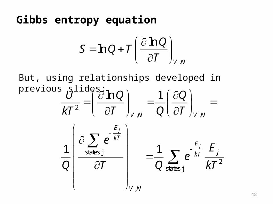
Gibbs entropy equation
But, using relationships developed in previous slides:
,
lnln
V N
QS Q T
T
2, ,
states j
2states j
,
ln 1
1 1
j
j
V N V N
E
kTE
jkT
V N
U Q Q
kT T Q T
eE
eQ T Q kT
48
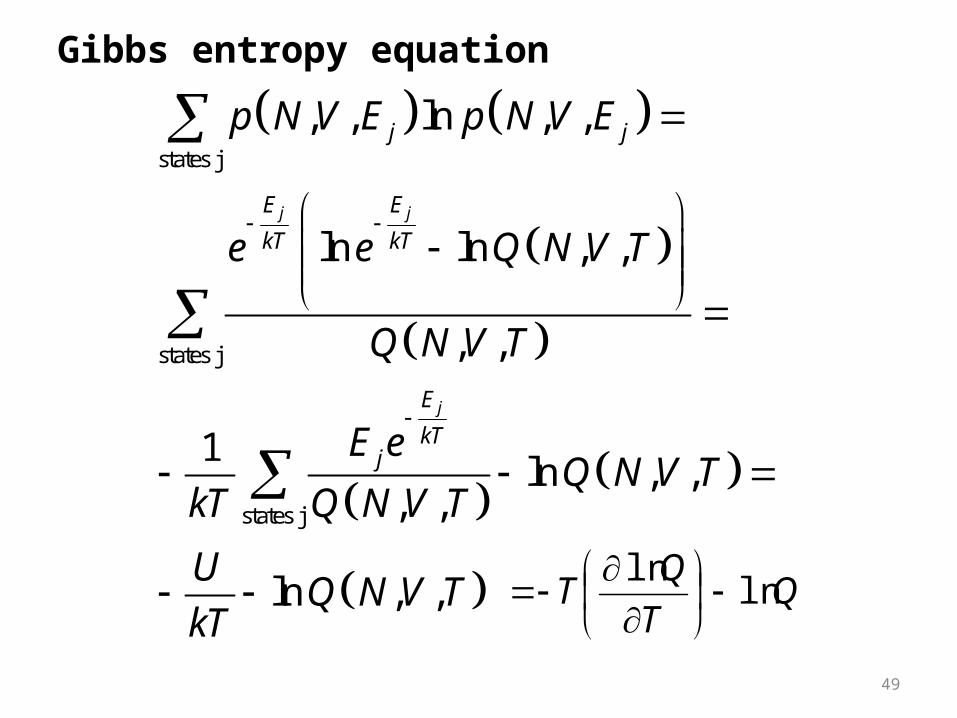
Gibbs entropy equation
states j
states j
states j
, , ln , ,
ln ln , ,
, ,
1ln , ,
, ,
ln , ,
j j
j
j j
E E
kT kT
E
kTj
p N V E p N V E
e e Q N V T
Q N V T
E eQ N V T
kT Q N V T
UQ N V T
kT
49
QT
QT ln
ln
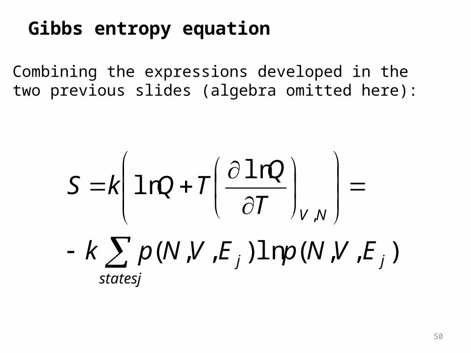
Gibbs entropy equation
Combining the expressions developed in the two previous slides (algebra omitted here):
50
),,(ln),,(
lnln
,
jstatesj
j
NV
EVNpEVNpk
T
QTQkS
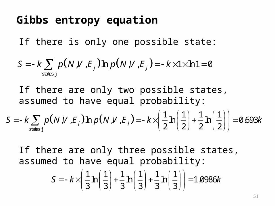
Gibbs entropy equation
If there is only one possible state:
states j
, , ln , , 1 ln1 0j jS k p N V E p N V E k
If there are only two possible states, assumed to have equal probability:
states j
1 1 1 1, , ln , , ln ln 0.693
2 2 2 2j jS k p N V E p N V E k k
If there are only three possible states, assumed to have equal probability:
1 1 1 1 1 1ln ln ln 1.0986
3 3 3 3 3 3S k k
51