The Hydrogen Atom The Resultant Force · The Resultant Force Consider three point charges located at the corners of a right triangle as shown in Figure below, where q 1 = q 3 = 5.0

Lesson 1 Electricity and Electrons • Electrostatics and coulomb’s law

Definitions Properties of Electric Charges Conductors , Insulators and Semiconductors Coulomb’s Law

The Hydrogen Atom The Resultant Force The Charge on the Spheres

• The Electric Field • Electric Field of a Continuous Charge Distribution • Electric Field Lines • Motion of Charged Particles in a Uniform Electric Field

Electrostatics and Coulomb’s Law

• Definitions Electric Charge - The charge is a property of certain elementary

particles, of which the most important are electrons and protons, both part of any atom of any material. The charge on a proton (the atomic nucleus of hydrogen) is called positive and written as e = 1.602· 10- 19

C. The charge of an electron is correspondingly called negative and written -e.

Electric Field - An electric field is defined as a region where an electric charge experiences an electric force acting upon it. The force F on a charge q in an electric field is proportional to the charge itself, and can thus be written

F=q·E E is called the electric field strength and is determined by the

magnitude and locations of the charges acting upon our charge q.


• Properties of Electric Charges

– charges of the same sign repel one another and charges with opposite signs attract one another.

– electric charge is always conserved in an isolated system.

Electrostatics and coulomb’s law

• Conductors , Insulators And Semiconductors

– Electrical conductors are materials in which some of the electrons are free electrons that are not bound to atoms and can move relatively freely through the material; electrical insulators are materials in which all electrons are bound to atoms and cannot move freely through the material.


• Coulomb’s Law

– The electric force – is inversely proportional to the square of the separation r

between the particles and directed along the line joining them;

– is proportional to the product of the charges q 1 and q 2 on the two particles;

– is attractive if the charges are of opposite sign and repulsive if the charges have the same sign;

– is a conservative force.


where ke is a constant called the Coulomb constant. The value of the Coulomb constant depends on the choice of units. The SI unit of charge is the coulomb (C). The Coulomb constant ke in SI units has the value

ke = 8.987 5 x 109 N.m2/C2

This constant is also written in the form

where the constant Є0 (lowercase Greek epsilon) is known as the permittivity of free space and has the value



• Example 1. The Hydrogen Atom

The electron and proton of a hydrogen atom are separated (on the average) by a distance of approximately 5.3 x10-11 m. Find the magnitudes of the electric force and the gravitational force between the two particles.

Solution From Coulomb’s law, we find that the magnitude of the electric force is


Using Newton’s law of universal gravitation

The ratio Fe /Fg = 2 x 1039.


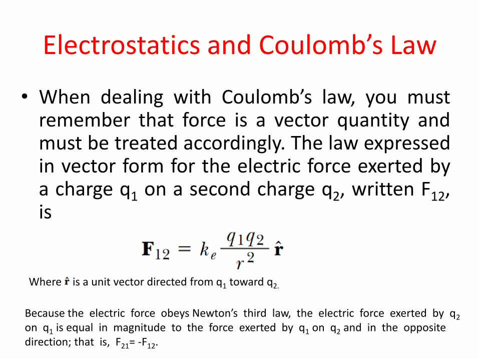
• When dealing with Coulomb’s law, you must remember that force is a vector quantity and must be treated accordingly. The law expressed in vector form for the electric force exerted by a charge q1 on a second charge q2, written F12, is

Where is a unit vector directed from q1 toward q2.

Because the electric force obeys Newton’s third law, the electric force exerted by q2 on q1 is equal in magnitude to the force exerted by q1 on q2 and in the opposite direction; that is, F21= -F12.


Vector form of Coulomb’s law

Two point charges separated by a distance r exert a force on each other that is given by Coulomb’s law. The force F21 exerted by q2 on q1 is equal in magnitude and opposite in direction to the force F12 exerted by q1 on q2. (a) When the charges are of the same sign, the force is repulsive. (b) When the charges are of opposite signs, the force is attractive.


• Example 2. The Resultant Force Consider three point charges located at the corners of a right triangle as shown in Figure below, where q1 = q3 = 5.0 μC, q2 = 2.0 μ C, and a = 0.10 m. Find the resultant force exerted on q3.

The force exerted by q1 on q3 is F13. The force exerted by q2 on q3 is F23. The resultant force F3 exerted on q3 is the vector sum F13 + F23.


Solution First, note the direction of the individual forces exerted by q1 and q2 on q3. The force F23 exerted by q2 on q3 is attractive because q2 and q3 have opposite signs. The force F13 exerted by q1 on q3 is repulsive because both charges are positive.

The magnitude of F23 is




• Example 3: The Charge on the Spheres Two identical small charged spheres, each having a mass of 3.0 X 10-2 kg, hang in equilibrium as shown in Figure below. The length of each string is 0.15 m, and the angle θ is 5.0°. Find the magnitude of the charge on each sphere.

(a) Two identical spheres, each carrying the same charge q, suspended in equilibrium. (b) The free-body diagram for the sphere on the left.


Solution

Electrostatics and Coulomb’s Law The separation of the spheres is 2a ! 0.026 m. From Coulomb’s law, the magnitude of the electric force is

The Electric Field

• An electric field is said to exist in the region of space around a charged object—the source charge. When another charged object—the test charge—enters this electric field, an electric force acts on it.

The Electric Field

A test charge q0 at point P is a distance r from a point charge q. (a) If q is positive, then the force on the test charge is directed away from q. (b) For the positive source charge, the electric field at P points radically outward from q. (c) If q is negative, then the force on the test charge is directed toward q. (d) For the negative source charge, the electric field at P points radially inward toward q.

The Electric Field

Thus, the electric field at point P due to a group of source charges can be expressed as the vector sum

The Electric Field

Example 4:Electric Field Due to Two Charges A charge q1 = 7.0 μC is located at the origin, and a second charge q2 =-5.0 μC is located on the x axis, 0.30 m from the origin. Find the electric field at the point P, which has coordinates (0, 0.40) m.

The total electric field E at P equals the vector sum E1+E2, where E1 is the field due to the positive charge q1 and E2 is the field due to the negative charge q2.

The Electric Field Solution

First, let us find the magnitude of the electric field at P due to each charge. The fields E1 due to the 7.0μC charge and E2 due to the -5.0μC charge are shown in the Figure. Their magnitudes are

The Electric Field

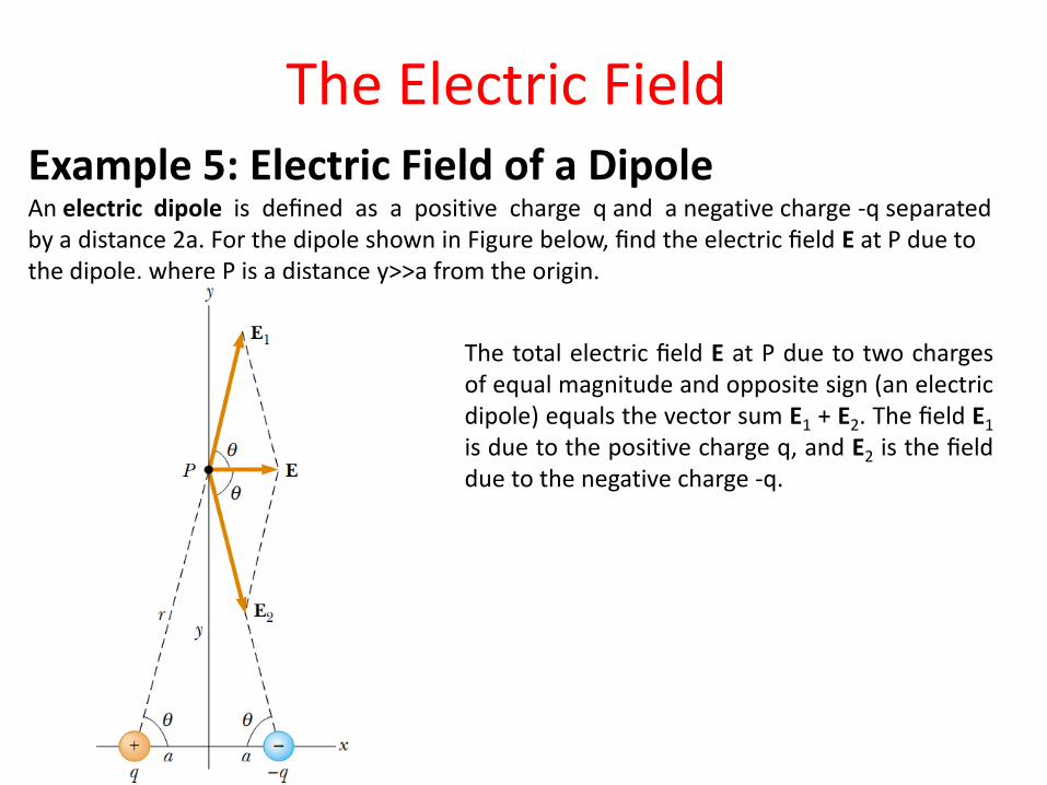
The Electric Field Example 5: Electric Field of a Dipole An electric dipole is defined as a positive charge q and a negative charge -q separated by a distance 2a. For the dipole shown in Figure below, find the electric field E at P due to the dipole, where P is a distance y>>a from the origin.

The total electric field E at P due to two charges of equal magnitude and opposite sign (an electric dipole) equals the vector sum E1 + E2. The field E1 is due to the positive charge q, and E2 is the field due to the negative charge -q.

The Electric Field

At P, the fields E1 and E2 due to the two charges are equal in magnitude because P is equidistant from the charges. The total field is E = E1 + E2, where

The y components of E1 and E2 cancel each other, and the x components are both in the positive x direction and have the same magnitude. Therefore, E is parallel to the x axis and has a magnitude equal to 2E1cosθ.

The Electric Field

Thus, we see that, at distances far from a dipole but along the perpendicular bisector of the line joining the two charges, the magnitude of the electric field created by the dipole varies as 1/r3, whereas the more slowly varying field of a point charge varies as 1/r2. This is because at distant points, the fields of the two charges of equal magnitude and opposite sign almost cancel each other. The 1/r3 variation in E for the dipole also is obtained for a distant point along the x axis and for any general distant point.

Electric Field of a Continuous Charge Distribution

Very often the distances between charges in a group of charges are much smaller than the distance from the group to some point of interest (for example, a point where the electric field is to be calculated). In such situations, the system of charges can be modeled as continuous. That is, the system of closely spaced charges is equivalent to a total charge that is continuously distributed along some line, over some surface, or throughout some volume. To evaluate the electric field created by a continuous charge distribution, we use the following procedure: first, we divide the charge distribution into small elements, each of which contains a small charge Δq, as shown in Figure (Next Page). we use Equation to calculate the electric field due to one of these elements at a point P. Finally, we evaluate the total electric field at P due to the charge distribution by summing the contributions of all the charge elements (that is, by applying the superposition principle). The electric field at P due to one charge element carrying charge Δq is


The electric field at P due to a continuous charge distribution is the vector sum of the fields ΔE due to all the elements Δq of the charge distribution




• Example 6: The Electric Field Due to a Charged Rod

A rod of length l has a uniform positive charge per unit

length λ and a total charge Q. Calculate the electric field at a point P that is located along the long axis of the rod and a distance a from one end




Tutorial 1

1. A disk of radius R has a uniform surface charge density σ. Calculate the electric field at a point P that lies along the central perpendicular axis of the disk and a distance x from the center of the disk.

2. A ring of radius a carries a uniformly distributed positive total charge Q. Calculate the electric field due to the ring at a point P lying a distance x from its center along the central axis perpendicular to the plane of the ring.

Electric Field Lines

The electric field lines for a point charge. (a) For a positive point charge, the lines are directed radially outward. (b) For a negative point charge, the lines are directed radially inward. Note

that the figures show only those field lines that lie in the plane of the page.


The electric field lines for two positive point charges The electric field lines for two point

charges of equal magnitude and opposite sign (an electric dipole)


Example 7: An Accelerated Electron

An electron enters the region of a uniform electric field as shown in Figure, with vi = 3.00 x 106 m/s and E = 200 N/C. The horizontal length of the plates is l = 0.100 m.


Documents

The Hydrogen Atom The Resultant Force · The Resultant Force Consider three point charges located at the corners of a right triangle as shown in Figure below, where q 1 = q 3 = 5.0