The huge Package for High-dimensional Undirected

Graph Estimation in R

Tuo Zhao ∗ Han Liu †

Kathryn Roeder ‡ John Lafferty § Larry Wasserman¶

January 26, 2012

Abstract

We describe an R package named huge which provides easy-to-use functions for

estimating high dimensional undirected graphs from data. This package implements

recent results in the literature, including Friedman et al. [2007b], Liu et al. [2009]

and Liu et al. [2010]. Compared with the existing graph estimation package glasso,

the huge package provides extra features: (1) instead of using Fortan, it is written

in C, which makes the code more portable and easier to modify; (2) besides fitting

Gaussian graphical models, it also provides functions for fitting high dimensional

semiparametric Gaussian copula models; (3) more functions like data-dependent

model selection, data generation and graph visualization; (4) a minor convergence

problem of the graphical lasso algorithm is corrected; (5) the package allows the

user to apply both lossless and lossy screening rules to scale up large-scale problems,

making a tradeoff between computational and statistical efficiency.

1 Overview

Undirected graphs is a natural approach to describe the conditional independence among

many variables. Each node of the graph represents a single variable and no edge between

two variables implies that they are conditional independent given all other variables.

In the past decade, significant progress has been made on designing efficient algorithms

to learn undirected graphs from high-dimensional observational datasets. Most of these

∗email: tzhao5@jhu.edu, Department of Computer Science, Johns Hopkins University†email: hanliu@cs.jhu.edu, Department of Biostatistics, Johns Hopkins University‡email: roeder@stat.cmu.edu, Department of Statistics, Carnegie Mellon University§email: lafferty@cs.cmu.edu, Machine Learning Department, Carnegie Mellon University¶email: larry@stat.cmu.edu, Department of Statistics, Carnegie Mellon University

1

methods are based on either the penalized maximum-likelihood estimation [Friedman

et al., 2007b] or penalized regression methods [Meinshausen and Buhlmann, 2006]. Ex-

isting packages include glasso, Covpath, CLIME and parcor. In particular, the glasso

package has been widely adopted by statisticians and computer scientists due to its

friendly user-inference and efficiency. There are also other graph estimation packages

such as GeneNet and sna, but they are not targeting on conditional independence graph

estimation.

In this vignette, we describe a newly developed R package named huge (High-dimensional

Undirected Graph Estimation). Compared with glasso, the core engine of huge is coded

in C, making modifications of the package more accessible to researchers from the com-

puter science and signal processing communities. The package includes a wide range

of functional modules, including data generation, data preprocessing, graph estimation,

model selection, and visualization. Many recent methods have been implemented, in-

cluding the nonparanormal [Liu et al., 2009] method for estimating a high dimensional

Gaussian copula graph, the StARS [Liu et al., 2010] approach for stability-based graph-

ical model selection, and correlation screening [Fan and Lv, 2008] for graph estimation.

The package supports two modes of screening, lossless [Witten et al., 2011, Mazumder

and Hastie, 2011a] and lossy screening. The user can select the desired screening level to

scale up to larger problems, but this introduces some estimation bias. This package also

addresses some minor convergence problem of the graphical lasso algorithm.

2 Background

2.1 Gaussian Graphical Models

The Gaussian Graphical Models assumes that the observations have a multivariate Gaus-

sian distribution with mean µ, and covariance matrix Σ.The conditional independence

can be implied by the inverse covariance (concentration) matrix Ω = Σ−1. If Ωjk = 0,

then the i-th variable and j-th variables are conditional independent given all other vari-

ables. Thus it makes sense to impose an ` penalty for the estimation of Ω, to increase its

sparsity, and the sparse pattern of Ω is essentially the same as the adjacency matrix of

the underlying undirected graph.

Meinshausen and Buhlmann [2006] take a simple approach to this problem and they

estimate a sparse graphical model by the following minimization problem,

G = argminG∈Rd×d,Gjj=0

1

2Tr(GTSG)− Tr(GTS) + λ‖G‖1 for all j = 1, ..., d (1)

where S denotes the sample covariance matrix and λ > 0 is the regularization parameter

controlling the sparsity level. (2.1) is equivalent to fitting lasso to each variable, using the

others as predictors. The component Ωij is then estimated to be non-zero if either the

2

estimated coefficient of variable i on j, (Gij), or the estimated coefficient of variable j on i,

(Gji), is non-zero (alternatively they use an AND rule), i.e. G has the same sparse pattern

as Ω. They show that asymptotically, this consistently estimates the sparse pattern of Ω.

Other authors have proposed algorithms for the exact maximization of the `1-penalized

log-likelihood and also formulates the estimation of Ω as a convex minimization problem,

Ω = argmaxΩ∈Rd×d,Ω0

log |Ω| − Tr(ΩTS)− λ‖Ω‖1 (2)

Banerjee et al. [2008] establish that the simpler approach of Meinshausen and Buhlmann

[2006] can be viewed as an approximation to the exact problem. While (2) can numerically

estimate Ω, which usually leads to more possible applications.

In our implementation of the package huge, we exploit many suggested tricks and

practices from Friedman et al. [2007b,a, 2010a]. We solve using coordinate descent and (2)

using block coordinate descent. They are both combined with active set and covariance

update tricks. We also modify the warm start trick to address the potential divergence

problem of the graphical lasso algorithm [Mazumder and Hastie, 2011b].

Remark 1. Meinshausen and Buhlmann [2006] is more efficient than Banerjee et al.

[2008] in computation, but the degrees of nodes for the estimation are usually restricted,

since we cannot get the non-zeros entries more than the sample size in each `1-regularized

regression problem.

Remark 2. Both Meinshausen and Buhlmann [2006] and Banerjee et al. [2008] can

asymptotically recover the true sparsity pattern under the irrepresentable condition and

a suitable choice of regularization. When the condition is violated or the regularization

parameter is not well tuned, it is highly difficult to achieve perfect recovery.

2.2 Gaussian Copula Models

Gaussian copula models extends the Gaussian graphical models by marginally trans-

forming the variables using smooth monotone functions. The underlying distribution is

still assumed to be d-variate Gaussian distribution N(0,Σ) by introducing a collection of

monotone functions fj’s such that (f1(X1), ..., fd(Xd))T ∼ N(0,Σ). The primary goal of

the nonparanormal is to estimate the underlying sample covariance matrix for a better

recovery of the underlying undirected graph [Liu et al., 2009].

Suppose we have n observations for j-th variable, x1j, ..., xnj, we sort all n observations

and get the corresponding rank u1j, ..., unj. Let Φ denote the Gaussian CDF function,

3

then we can estimate the transformed data using:

fj(xij) = Φ−1(uij)︸ ︷︷ ︸The normal score

or fj(xij) =

Φ−1(δ) if uij ≤ δ

Φ−1(uij) if δ < uij ≤ 1− δΦ−1(1− δ) if uij > 1− δ

︸ ︷︷ ︸The truncated normal

(3)

where

uij =uijn+ 1

and δ =1

4n1/4√π log n

. (4)

2.3 Screening

Although efficient algorithms have been developed, it is still very difficult to efficiently

solve large scale problem. In the past few years, several fast screening method have been

proposed to address the fast pre-selection before graph estimation. They aim to first

reduce the high dimension to the moderate size with the informative variables preserved.

Then the refined algorithm can be further applied.

In our implementation, we provide an optional procedure Fan and Lv [2008] to Mein-

shausen and Buhlmann [2006]. In each lasso problem, we can select the variables having

larger sample correlation with the response. Since Fan and Lv [2008] only guarantee

under certain regularity condition, it can preserve the informative variables with a large

probability. We refer it as the lossy screening rule.

We further extended Fan and Lv [2008] to Friedman et al. [2007b]. If Sij ≤ λ, then

we will set no edge between the i-th and j-th variable. In fact the graph generated by our

lossy screening based on correlation can also roughly approximate the underlying partial

correlation graph Friedman et al. [2010a]. Due to its low computational cost, it has been

widely applied in biomedical research [Langfelder and Horvath, 2008].

Witten et al. [2011], Mazumder and Hastie [2011b] also establish a very simple rule

to pre-select the nodes before graph estimation. If Sij ≤ λ for all j 6= i, then the i-th

variable will be a isolated node in the final estimator. Eventually we only need to estimate

a small block of the inverse covariance matrix. This screening rule is derived from the

perspective of convex optimization (KKT condition), and doesn’t affect the statistical

efficacy. We refer it to the lossless screening rule.

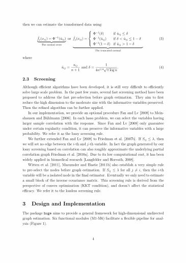
3 Design and Implementation

The package huge aims to provide a general framework for high-dimensional undirected

graph estimation. Six functional modules (M1-M6) facilitate a flexible pipeline for anal-

ysis (Figure 1).

4

Nonparanormal Graph estimation with the lossless screening rule

Graph estimation with the lossy screening rule

scr Model selection

Visualization Data No

Yes M1 M2 M3

M4

M5 M6

Figure 1: The graph estimation pipeline.

M1. Data Generator: The function huge.generator() can generate multivariate

Gaussian data with different undirected graph structures, including hub, cluster, band,

scale-free, and Erdos-Renyi random graphs. The sparsity level of the graph structures

and signal-to-noise ratios can also be adjusted by users.

M2. Semiparametric Transformation: The function huge.npn() implements the

nonparanormal method [Liu et al., 2009] for estimating a semiparametric Gaussian cop-

ula model by truncated normal or normal score. Computationally, the estimation of a

nonparanormal transformation only requires one pass through the data matrix.

Remark 3. Although in the existing high-dimensional theory, the truncation has been

proved to be asymptotically consistent and no corresponding result has been established

for normal score, we find the normal score also has a good performance in practice.

M3. Graph Screening: The scr argument in the main function huge() controls the

use of large-scale correlation screening before graph estimation. The function supports

two types of screening rules,lossless screening and lossy screening. The lossless screening

method is from Witten et al. [2011], Mazumder and Hastie [2011b] and the lossy screening

method is from Fan and Lv [2008]. Such screening procedures can greatly reduce the

computational cost and achieve equal or even better estimation by reducing the variance

at the expense of an increase in bias.

M4. Graph Estimation: Similar to the glasso package, the method argument in

the huge() function supports two estimation methods: (i) the Meinshausen-Buhlmann

covariance selection algorithm [Meinshausen and Buhlmann, 2006] and (ii) the graphical

lasso algorithm [Friedman et al., 2007b, Banerjee et al., 2008]. One difference between

huge and glasso is that we implement all the core components using C instead of For-

tran. The code is also memory-optimized using sparse matrix data structures so that

it can handle larger datasets when estimating and storing full regularization paths. We

also provide an additional graph estimation method based on thresholding the sample

correlation matrix. Such an approach is computationally efficient and has been widely

applied in biomedical research [Langfelder and Horvath, 2008].

Remark 4. We find the graphical lasso algorithm may fail to converge using the warm

start trick when estimating the solution path. We proposed a modified warm start trick

and explained the reason of the failure for the original warm start trick in the Appendix.

5

M5. Model Selection: The function huge.select() provides three regularization

parameter selection methods: the stability approach for regularization selection (StARS)

[Liu et al., 2010]; a modified rotation information criterion (RIC) [Lysen, 2009]; and the

extended Bayesian information criterion [Foygel and Drton, 2010]. The latter approach is

a likelihood-based model selection criterion that is only applicable for the graphical lasso

method. StARS conducts many subsampling steps to calculate variability score using

the U-statistics, which is computationally intensive but can be trivially parallelized. RIC

is closely related to the permutation approach for model selection and scales to large

datasets.

Remark 5. Under certain regularity condition, StARS is partially consistent and suffers

overselection. The performance of StARS also depends on the tuning grid chosen by user.

Remark 6. RIC randomly rotates the variables for each sample multiple times and selects

the minimum regularization which generates all zero estimated using rotated data. It has

no theoretical guarantee of the consistent recovery and often suffers serious underselection

or overselection.

M6. Graph Visualization: The plotting functions huge.plot() and plot() provide

visualizations of the simulated data sets, estimated graphs and paths. The implementa-

tion is based on the igraph package. Due to the limits of igraph, sparse graphs with

only up to 2,000 nodes can be visualized.

4 User Interface by Example

We illustrate the user interface by two simple examples. The first one is based on the

simulated data generated by huge.generator(),

> library(huge) # Load the package huge

> L = huge.generator(n=200,d=200,graph="hub") # Generate data with hub structures

> X = L$data; X.pow = X^3/sqrt(15) # Power Transformation

> X.npn = huge.npn(X.pow) # Nonparanormal

> out.mb = huge(X.pow,nlambda=30) # Estimate the solution path

> out.npn = huge(X.npn,nlambda=30)

> huge.roc(out.mb$path,L$theta) # Plot the ROC curve

> huge.roc(out.npn$path,L$theta)

> mb.stars = huge.select(out.mb,criterion="stars",

+ stars.thresh=0.05) # Select the graph using StARS

> npn.stars = huge.select(out.npn,criterion="stars",stars.thresh=0.05)

> mb.ric = huge.select(out.mb) # Select the graph using RIC

> npn.ric = huge.select(out.npn)

6

0.00 0.05 0.10 0.15 0.20 0.25 0.30 0.35

0.0

0.2

0.4

0.6

0.8

1.0

ROC Curve

False Postive Rate

True

Pos

tive

Rat

e

(a) The ROC curve (b) The optimal graph byStARS

(c) The optimal graph by RIC

Figure 2: Simulated results w/o nonparanormal

0.00 0.05 0.10 0.15 0.20 0.25 0.30 0.35

0.0

0.2

0.4

0.6

0.8

1.0

ROC Curve

False Postive Rate

True

Pos

tive

Rat

e

(a) The ROC curve (b) The optimal graph byStARS

(c) The optimal graph by RIC

Figure 3: Simulated results w/ nonparanormal

We generate 200 samples following a 200-dimensional Gaussian distribution with the

hub structure, then transform the data using power transformation, which preserves

the population mean and population variance. The graph is estimated by Meinshausen

and Buhlmann [2006] by default. The program automatically sets up a sequence of 30

regularization parameters and estimates the corresponding graph path. The results w/o

and w/ non paranormal are shown in Figure 2 and Figure 3 respectively. We can see a

significant improvement by using nonparanormal. As mentioned in the previous section,

the StARS and RIC yields a overselected and a underselected graph respectively.

The second example is based on a stock market data which we contribute to the huge

package. We acquired closing prices from all stocks in the S&P 500 for all the days that

the market was open between January 1, 2003 and January 1, 2008. This gave us 1258

samples for the 452 stocks that remained in the S&P 500 during the entire time period.

> data(stockdata) # Load the stock data

> Y = log(stockdata$data[2:1258,]/stockdata$data[1:1257,]) # Preprocessing

Here the data have been transformed by calculating the log-ratio of the price at time t

to price at time t− 1, and then standardized by subtracting the mean and adjusting the

variance to one.

> Y.npn = huge.npn(Y, npn.func="truncation") # Nonparanormal

7

> out.npn = huge(Y.npn,method = "glasso", nlambda=40,lambda.min.ratio = 0.4)

> out = huge(Y,method = "glasso", nlambda=40,lambda.min.ratio = 0.4)

Here the nonparanormal transformation is applied to the data, and the graph is estimated

using the graphical lasso (the default is the Meinshausen-Buhlmann estimator). The pro-

gram automatically sets up a sequence of 40 regularization parameters and estimates the

corresponding graph path. The lossless screening method is applied by default. The out-

put of graph estimation using the transformed data is shown in Figure 4. To investigate

0.8 0.6 0.4

0.00

0.04

0.08

Sparsity

Regularization

x$sparsity

lambda = 0.664

lambda = 0.605

lambda = 0.538

Figure 4: The estimated graph path.

the impact of the nonparanormal transformation, we plot points in a subgraph calculated

with and without the transformation (Figure 5). Both graphs have the sparsity level at

!

!

!

!

!

!

!

!

!

!

!

!

!

!!

!!

!

!

!

!

!

!

!

!

!

!

!

!

!

!

!

!

!

!

!

!

!

!

!

!

!

!

!

!!

!

!

!

!!

!

!

!

!

!

!

!!

!

!

!

!

!

!

!

!

!

!!!

!

!!

!

!! !

!

!

!

!

!

!

!

!

!

!

!

!

!

!

!

!!

!

!

!

!

!

!!

!

!

!

!

!

!

!

!

!

!

!

!

!

!

!

!

!

!

! !

!

!

!

!

!

!

!

!

!

!

!!

!

!

!

!

!

!

!

!

!

!

!

!

!

!

!

!

!

!

!

!

!

!

!

!

!

!!

!!

!

!

!

!!

!

!

!

!

!

!

!

!!

!

!

!

!

!

!

!

!

!

!!

!

!

!

!

!!

!

!

!

!

!

!

!

!

!

!

!

!

!

!

!

!

!

!

!

!

!

!

!

!

!

!

!

!

!

!

!

!

!

!

!

!!

!

!

!!

!

!

!

!

!

!

!

!

!

!

!

!

!!

!

!

!

! !

!

!

!

!

!

!

!

!

!

!

!

!

!!

!!

!

!

!

!

!

!

!

!

!

!

!

!

!

!

!

!

!

!

!

!

!

!

!

!

!

!

!

!!

!

!

!

!!

!

!

!

!

!

!

!!

!

!

!

!

!

!

!

!

!

!!!

!

!!

!

!! !

!

!

!

!

!

!

!

!

!

!

!

!

!

!

!

!!

!

!

!

!

!

!!

!

!

!

!

!

!

!

!

!

!

!

!

!

!

!

!

!

!

! !

!

!

!

!

!

!

!

!

!

!

!!

!

!

!

!

!

!

!

!

!

!

!

!

!

!

!

!

!

!

!

!

!

!

!

!

!

!!

!!

!

!

!

!!

!

!

!

!

!

!

!

!!

!

!

!

!

!

!

!

!

!

!!

!

!

!

!

!!

!

!

!

!

!

!

!

!

!

!

!

!

!

!

!

!

!

!

!

!

!

!

!

!

!

!

!

!

!

!

!

!

!

!

!

!!

!

!

!!

!

!

!

!

!

!

!

!

!

!

!

!

!!

!

!

!

!

Figure 5: The estimated glasso graph (left) and nonparanormal graph (right).

about 1% and we can see the different pattern between them. We highlight a dense mod-

ule in the nonparanormal graph which is much sparser in the corresponding glasso graph.

We can see all nodes in this module belong to the same category. This example well

demonstrates the power of the nonparanormal method to reveal the relationship beyond

the normality assumption.

8

5 Performance Benchmark

We adopt similar experimental settings as in Friedman et al. [2010b] to compare huge

with glasso (ver 1.4). We consider four scenarios with varying sample sizes n and

number of variables d, as shown in Table 1. We simulate the data from three different

multivariate normal distributions with null graph (diagonal covariance matrix) and Erdos-

Renyi random graph (with probability 0.01 )structures respectively. Timings (in seconds)

are computed over 10 values of the corresponding regularization parameter, and the range

of regularization parameters is chosen so that each method produced approximately the

same number of non-zero estimates. The convergence threshold of both glasso and huge

is chosen to be 10−4. All experiments were carried out on a PC with Intel Core i5 3.3GHz

processor. Unfortunately, CLIME (ver 1.0) Covpath (ver 0.2), were unable to obtain timing

results due to numerical issues. parcor (ver 0.22) failed to get any results in 3 hours.

Table 1: Experimental Results on Null Graph

Methodd = 1000 d = 2000 d = 3000 d = 4000n = 100 n = 150 n = 200 n = 300

huge-Meinshausen-Buhlmann (lossy) 2.688 (0.140) 11.14 (0.623) 30.47 (0.738) 223.5 (13.14)huge-Meinshausen-Buhlmann 4.032 (0.267) 37.51 (2.254) 119.6 (3.888) 330.6 (25.49)glasso-Meinshausen-Buhlmann 34.38 (0.481) 245.8 (4.143) 800.7 (7.652) 2694 (136.5)huge-graphical lasso (lossy) 34.39 (2.173) 246.5 (16.18) 857.3 (24.18) 2015 (151.1)huge-graphical lasso (lossless) 43.13 (3.461) 310.4 (28.19) 1071 (41.51) 2510 (293.4)glasso-graphical lasso 122.1 (5.259) 931.4 (45.96) 2998 (97.71) 7485 (307.5)

For Meinshausen-Buhlmann graph estimation, we can see that huge achieves the best

performance. In particular, when the lossy screening rule is applied, huge automatically

reduces each individual lasso problem from the original dimension d to the sample size

n, therefore even better efficiency can be achieved in settings when d n. Based on our

experiments, the speed up due to the lossy screening rule can be up to 400%.

Table 2: Experimental Results on Random Graph

Methodd = 1000 d = 2000 d = 3000 d = 4000n = 100 n = 150 n = 200 n = 300

huge-Meinshausen-Buhlmann (lossy) 3.246 (0.147) 13.47 (0.665) 35.87 (0.97) 247.2 (14.26)huge-Meinshausen-Buhlmann 4.24 (0.288) 42.41 (2.338) 147.9 (4.102) 357.8 (28.00)glasso-Meinshausen-Buhlmann 37.23 (0.516) 296.9 (4.533) 850.7 (8.180) 3095 (150.5)huge-graphical lasso (lossy) 39.61 (2.391) 289.9 (17.54) 905.6 (25.84) 2370 (168.9)huge-graphical lasso (lossless) 47.86 (3.583) 328.2 (30.09) 1276 (43.61) 2758 (326.2)glasso-graphical lasso 131.9 (5.816) 1054 (47.52) 3463 (107.6) 8041 (316.9)

Unlike the Meinshausen-Buhlmann graph approach, the graphical lasso estimates the

inverse covariance matrix. The lossless screening rule [Witten et al., 2011, Mazumder and

Hastie, 2011b] greatly reduces the computation required by the graphical lasso algorithm,

especially when the estimator is highly sparse. The lossy screening rule can further speed

up the algorithm and provides an extra performance boost.

9

6 Conclusions

We developed a new package named huge, for high dimensional undirected graph estima-

tion. The package is complementary to the existing glasso package by providing extra

features and functional modules. We plan to maintain and support this package in the

future.

7 Appendix

7.1 A Typical Example of Failure

In the package glasso, the warm start trick begins with the larger regularization parame-

ters and gradually decreases the regularization parameter. However, in real applications,

we find this strategy may lead to divergence or other numerical issues sometimes. We

first provide an example that glasso fails to converge.

> library(huge) # load the package huge

> library(glasso) # Load the package glasso

> data(stockdata) # Load the stock data

> X = log(stockdata$data[2:1258,]/stockdata$data[1:1257,]) # Preprocessing

> out.huge = huge(X,method = "glasso", nlambda=5)

> out.glasso = glassopath(cor(X),rholist = out.huge$lambda[5:1])

7.2 A Modified Warm Start trick

From Banerjee et al. [2008], we know a good initial value for the estimated covariance

matrix Σ should satisfy the constraint

‖Σ− S‖∞ ≤ λ and Σ 0 (5)

where S is the sample covariance matrix. Otherwise, the algorithm cannot guarantee the

positive definiteness of the estimation. Once the positive definiteness is violated in some

iteration, the whole algorithm will fail. Now suppose we have a sequence of decreasing

regularization parameters λ1, ..., λK and for λk, we have obtain the estimated covariance

matrix as Σk. By KKT condition, we know

‖Σk − S‖∞ ≤ λk (6)

However, when we use Σk as the initial values for estimating Σk+1 corresponding to λk+1,

although Σk 0 hold, it is highly likely that Σk may violate our requirement of (5)

when using the regularization parameter λk+1, since λk > λk+1. The glass algorithm may

tolerate slight violation sometimes, but when we decrease the regularization parameter

10

too fast, then a failure is highly likely to happen. The phenomenon was also found

independently by Mazumder and Hastie [2011b].

In our implementation of the graphical lasso, we actually take the initial covariance

matrix as the sample covariance matrix and compute the path using the regularization

parameters in the increasing order. We sacrifice a little bit efficiency, but guarantee our

huge won’t fail due to the warm start trick. Although our strategy is quite counterintu-

itive, but it works well in practice. In the previous example, huge successful estimated

the solution path for only seconds, while glasso showed no intent to stop, thus we killed

the corresponding process after 3 hours.

References

O. Banerjee, L. E. Ghaoui, and A. d’Aspremont. Model selection through sparse maxi-

mum likelihood estimation. Journal of Machine Learning Research, 9:485–516, 2008.

T. Cai, W. Liu, and X. Luo. A constrained l1 minimization approach to sparse precision

matrix estimation. Technical report, University of Pennsylvania, 2010.

J. Fan and J. Lv. Sure independence screening for ultrahigh dimensional feature space.

Journal of the Royal Statistical Society Series B, 70:849–911, 2008.

R. Foygel and M. Drton. Extended Bayesian information criteria for Gaussian graphical

models. Advances in Neural Information Processing Systems, 2010.

J. Friedman, T. Hastie, H. Hofling, and R. Tibshirani. Pathwise coordinate optimization.

Annals of Applied Statistics, 1(2), 2007a.

J. Friedman, T. Hastie, and R. Tibshirani. Sparse inverse covariance estimation with the

graphical lasso. Biostatistics, 9(3):432–441, 2007b.

J. Friedman, T. Hastie, and R. Tibshirani. Regularization paths for generalized linear

models via coordinate descent. Journal of Statistical Software, 33(1), 2010a.

J. Friedman, T. Hastie, and R. Tibshirani. Applications of the lasso and grouped lasso

to the estimation of sparse graphical models. Technical report, Stanford University,

2010b.

Vijay Krishnamurthy and Alexandre d’Aspremont. A pathwise algorithm for covariance

selection. Optimization for Machine Learning, 2011.

P. Langfelder and S. Horvath. WGCNA: An R package for weighted correlation network

analysis. BMC Bioinformatics, 9, 2008.

11

H. Liu, J. Lafferty, and L. Wasserman. The nonparanormal semiparametric estimation

of high dimensional undirected graphs. Journal of Machine Learning Research, 10:

2295–2328, 2009.

H. Liu, K. Roeder, and L. Wasserman. Stability approach to regularization selection

for high dimensional graphical models. Advances in Neural Information Processing

Systems, 2010.

S. Lysen. Permuted Inclusion Criterion: A Variable Selection Technique. PhD thesis,

University of Pennsylvania, 2009.

R. Mazumder and T. Hastie. Exact covariance thresholding into connected components

for large-scale graphical lasso. Technical report, Stanford University, 2011a.

R. Mazumder and T. Hastie. The graphical lasso: New insights and alternatives. Tech-

nical report, Stanford University, 2011b.

N. Meinshausen and P. Buhlmann. High dimensional graphs and variable selection with

the lasso. Annals of Statistics, 34(3):1436–1462, 2006.

D. Witten, J. Friedman, and Noah Simon. New insights and faster computations for the

graphical lasso. Journal of Computational and Graphical Statistics, to appear, 2011.

12