© 2

018

Nat

ure

Am

eric

a, In

c., p

art o

f Spr

inge

r Nat

ure.

All

right

s re

serv

ed.

NATURE NEUROSCIENCE VOLUME 20 | NUMBER 11 | NOVEMBER 2017 1643

A R T I C L E S

Learning to predict long-term reward is fundamental to the survival of many animals. Some species may go days, weeks, or even months before attaining primary reward, during which time aversive states must be endured. Evidence suggests that the brain has evolved mul-tiple solutions to this reinforcement learning (RL) problem1. One solution is to learn a model or cognitive map of the environment2, which can then be used to generate long-term reward predictions through simulation of future states1. However, this solution is com-putationally intensive, especially in real-world environments where the space of future possibilities is virtually infinite. An alternative, model-free solution is to learn, from trial-and-error, a value function that maps states to long-term reward predictions3. However, dynamic environments can be problematic for this approach, because changes in the distribution of rewards necessitate complete relearning of the value function.

Here we argue that the hippocampus supports a third solution: learning of a predictive map that represents each state in terms of its successor states4. This representation is sufficient for long-term reward prediction, is learnable using a simple, biologically plausible algorithm, and explains a wealth of data from studies of the hippocampus.

Our primary focus is on understanding the computational function of hippocampal place cells, which respond selectively when an animal occupies a particular location in space5. A classic and still influential view of place cells is that they collectively furnish an explicit map of space5. This map can then be employed as the input to a model-based6,7 or model-free8,9 RL system for computing the value of the animal’s current state. In contrast, the predictive map theory views place cells as encoding predictions of future states, which can then be combined with reward predictions to compute values. This theory can account for why the firing of place cells is modulated by variables like obstacles, environment topology, and direction of travel. It also gener-alizes to hippocampal coding in nonspatial tasks. Beyond the hippoc-ampus, we argue that entorhinal grid cells10, which fire periodically over space, encode a low-dimensional decomposition of the predictive map, useful for stabilizing the map and discovering subgoals.

RESULTSThe successor representationAn animal’s optimal course of action will frequently depend on the location (or more generally, the ‘state’) that the animal is in. The hippocampus’ purported role in representing location is therefore considered to be a very important one. The traditional view of state representation in the hippocampus is that the place cells index the cur-rent location by firing when the animal visits the encoded location and otherwise remain silent5. The main idea of the successor representation (SR) model, elaborated below, is that place cells do not encode place per se but rather a predictive representation of future states given the current state. Thus, two physically adjacent states that predict divergent future states will have dissimilar representations, and two states that predict similar future states will have similar representations.

The SR emerges naturally from the definition of value (V) often used in RL. The value of a current state s is defined as the expected sum of the reward at each future state st, multiplied by an exponentially decay-ing discount factor [0, 1] that downweights distal rewards:

V s R s s st

tt( ) ( ) | ( )

00 1g

where st is the state visited at time t (see Online Methods for formal mathematical detail).

The value function can be decomposed into the inner product of the reward function with a predictive representation of the state (the SR)4, denoted by M:

V s M s s R ss

( ) ( , ) ( ), ( )2

The SR encodes the expected discounted future occupancy of state s along a trajectory initiated in state s:

M s s s s s st

tt( , ) | ( )

00 3g

(1)(1)

(2)(2)

(3)(3)

1DeepMind, London, UK. 2Princeton Neuroscience Institute, Princeton University, Princeton, New Jersey, USA. 3Gatsby Computational Neuroscience Unit, University College London, London, UK. 4Department of Psychology and Center for Brain Science, Harvard University, Cambridge, Massachusetts, USA. Correspondence should be addressed to K.L.S. (stachenfeld@google.com).

Received 19 December 2016; accepted 29 August 2017; published online 02 October 2017; corrected online 25 April 2018; doi:10.1038/nn.4650

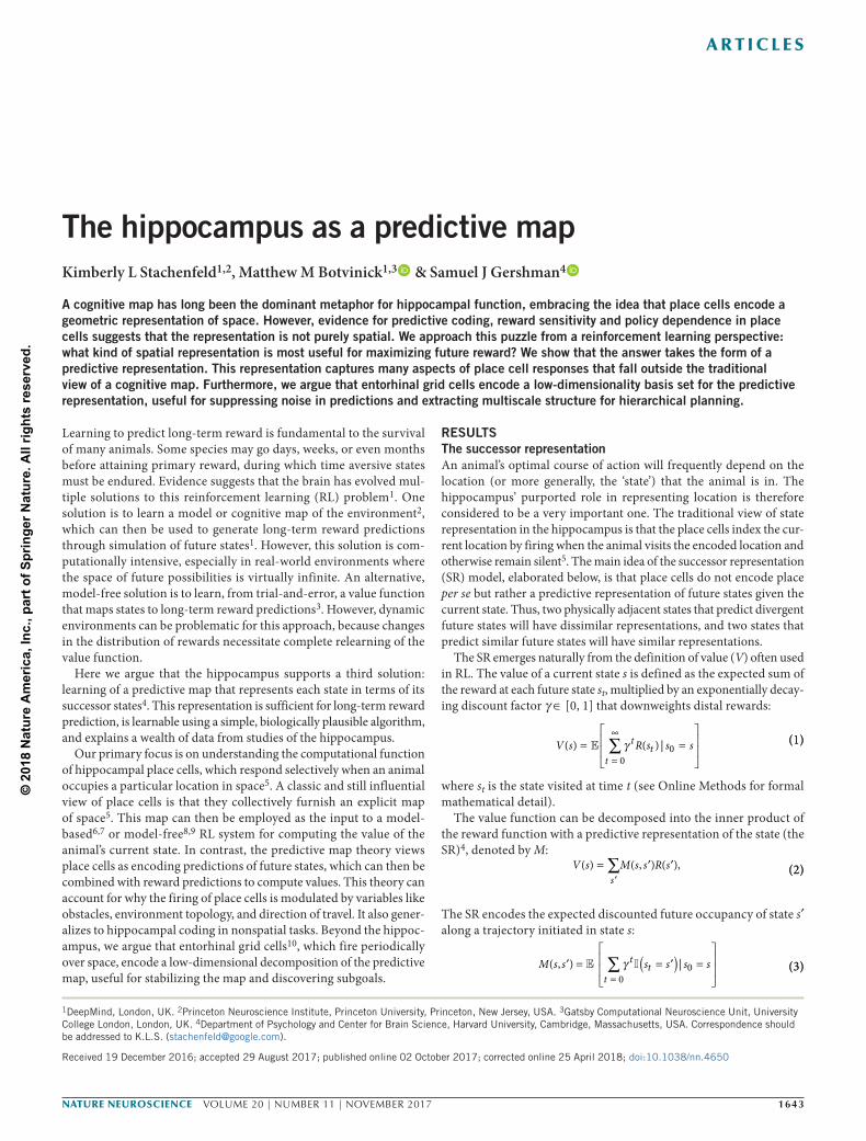
The hippocampus as a predictive mapKimberly L Stachenfeld1,2, Matthew M Botvinick1,3 & Samuel J Gershman4

A cognitive map has long been the dominant metaphor for hippocampal function, embracing the idea that place cells encode a geometric representation of space. However, evidence for predictive coding, reward sensitivity and policy dependence in place cells suggests that the representation is not purely spatial. We approach this puzzle from a reinforcement learning perspective: what kind of spatial representation is most useful for maximizing future reward? We show that the answer takes the form of a predictive representation. This representation captures many aspects of place cell responses that fall outside the traditional view of a cognitive map. Furthermore, we argue that entorhinal grid cells encode a low-dimensionality basis set for the predictive representation, useful for suppressing noise in predictions and extracting multiscale structure for hierarchical planning.

© 2

018

Nat

ure

Am

eric

a, In

c., p

art o

f Spr

inge

r Nat

ure.

All

right

s re

serv

ed.

1644 VOLUME 20 | NUMBER 11 | NOVEMBER 2017 NATURE NEUROSCIENCE

A R T I C L E S

where (st = s ) = 1 if st = s and 0 otherwise. Thus, we decompose the expected discounted reward into expected discounted future state occupancy and the reward at each state. An estimate of the SR (denoted M̂ ) can be incrementally updated using a form of the temporal difference learning algorithm (equation (8))4,11.

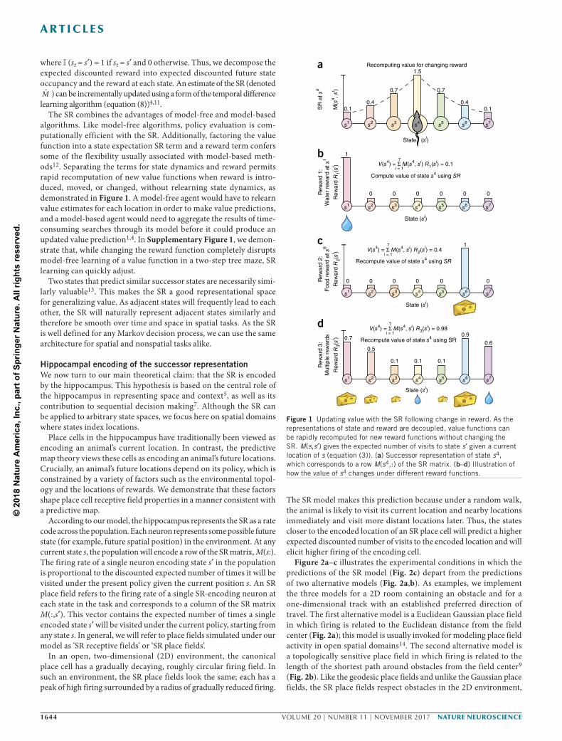
The SR combines the advantages of model-free and model-based algorithms. Like model-free algorithms, policy evaluation is com-putationally efficient with the SR. Additionally, factoring the value function into a state expectation SR term and a reward term confers some of the flexibility usually associated with model-based meth-ods12. Separating the terms for state dynamics and reward permits rapid recomputation of new value functions when reward is intro-duced, moved, or changed, without relearning state dynamics, as demonstrated in Figure 1. A model-free agent would have to relearn value estimates for each location in order to make value predictions, and a model-based agent would need to aggregate the results of time- consuming searches through its model before it could produce an updated value prediction1,4. In Supplementary Figure 1, we demon-strate that, while changing the reward function completely disrupts model-free learning of a value function in a two-step tree maze, SR learning can quickly adjust.

Two states that predict similar successor states are necessarily simi-larly valuable13. This makes the SR a good representational space for generalizing value. As adjacent states will frequently lead to each other, the SR will naturally represent adjacent states similarly and therefore be smooth over time and space in spatial tasks. As the SR is well defined for any Markov decision process, we can use the same architecture for spatial and nonspatial tasks alike.

Hippocampal encoding of the successor representationWe now turn to our main theoretical claim: that the SR is encoded by the hippocampus. This hypothesis is based on the central role of the hippocampus in representing space and context5, as well as its contribution to sequential decision making7. Although the SR can be applied to arbitrary state spaces, we focus here on spatial domains where states index locations.

Place cells in the hippocampus have traditionally been viewed as encoding an animal’s current location. In contrast, the predictive map theory views these cells as encoding an animal’s future locations. Crucially, an animal’s future locations depend on its policy, which is constrained by a variety of factors such as the environmental topol-ogy and the locations of rewards. We demonstrate that these factors shape place cell receptive field properties in a manner consistent with a predictive map.

According to our model, the hippocampus represents the SR as a rate code across the population. Each neuron represents some possible future state (for example, future spatial position) in the environment. At any current state s, the population will encode a row of the SR matrix, M(s:). The firing rate of a single neuron encoding state s in the population is proportional to the discounted expected number of times it will be visited under the present policy given the current position s. An SR place field refers to the firing rate of a single SR-encoding neuron at each state in the task and corresponds to a column of the SR matrix M(:,s ). This vector contains the expected number of times a single encoded state s will be visited under the current policy, starting from any state s. In general, we will refer to place fields simulated under our model as ‘SR receptive fields’ or ‘SR place fields’.

In an open, two-dimensional (2D) environment, the canonical place cell has a gradually decaying, roughly circular firing field. In such an environment, the SR place fields look the same; each has a peak of high firing surrounded by a radius of gradually reduced firing.

The SR model makes this prediction because under a random walk, the animal is likely to visit its current location and nearby locations immediately and visit more distant locations later. Thus, the states closer to the encoded location of an SR place cell will predict a higher expected discounted number of visits to the encoded location and will elicit higher firing of the encoding cell.

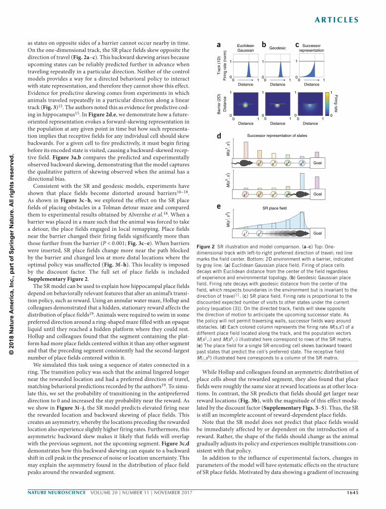
Figure 2a–c illustrates the experimental conditions in which the predictions of the SR model (Fig. 2c) depart from the predictions of two alternative models (Fig. 2a,b). As examples, we implement the three models for a 2D room containing an obstacle and for a one-dimensional track with an established preferred direction of travel. The first alternative model is a Euclidean Gaussian place field in which firing is related to the Euclidean distance from the field center (Fig. 2a); this model is usually invoked for modeling place field activity in open spatial domains14. The second alternative model is a topologically sensitive place field in which firing is related to the length of the shortest path around obstacles from the field center9 (Fig. 2b). Like the geodesic place fields and unlike the Gaussian place fields, the SR place fields respect obstacles in the 2D environment,

1

s1 s2 s3 s4 s5 s6 s7

Rew

ard

1:W

ater

rew

ard

at s

1R

ewar

d 2:

Foo

d re

war

d at

s6

Rew

ard

3:M

ultip

le r

ewar

ds

1.5

0.10.4

0.7

0.10.4

0.7

1

0 0 0 0 0 0

0 0 0 0 0 0

0.1 0.1 0.1

0.5

0.7 0.90.6

Recomputing value for changing rewarda

b

c

d

State (si)

s1 s2 s3 s4 s5 s6 s7

s1 s2 s3 s4 s5 s6 s7

s1 s2 s3 s4 s5 s6 s7

Rew

ard

R1(

si )

Compute value of state s4 using SR

Recompute value of state s4 using SR

State (si)

State (si)

State (si)

Rew

ard

R3(

si )

SR

at s

4

M(s

4 , si )

V(s4) = M(s4, si) R1(si) = 0.17

i = 1

Rew

ard

R2(

si ) V(s4) = M(s4, si) R2(si) = 0.4i = 1

7

Recompute value of state s4 using SR

V(s4) = M(s4, si) R3(si) = 0.987

i = 1

Figure 1 Updating value with the SR following change in reward. As the representations of state and reward are decoupled, value functions can be rapidly recomputed for new reward functions without changing the SR. M(s,s ) gives the expected number of visits to state s given a current location of s (equation (3)). (a) Successor representation of state s4, which corresponds to a row M(s4,:) of the SR matrix. (b–d) Illustration of how the value of s4 changes under different reward functions.

© 2

018

Nat

ure

Am

eric

a, In

c., p

art o

f Spr

inge

r Nat

ure.

All

right

s re

serv

ed.

NATURE NEUROSCIENCE VOLUME 20 | NUMBER 11 | NOVEMBER 2017 1645

A R T I C L E S

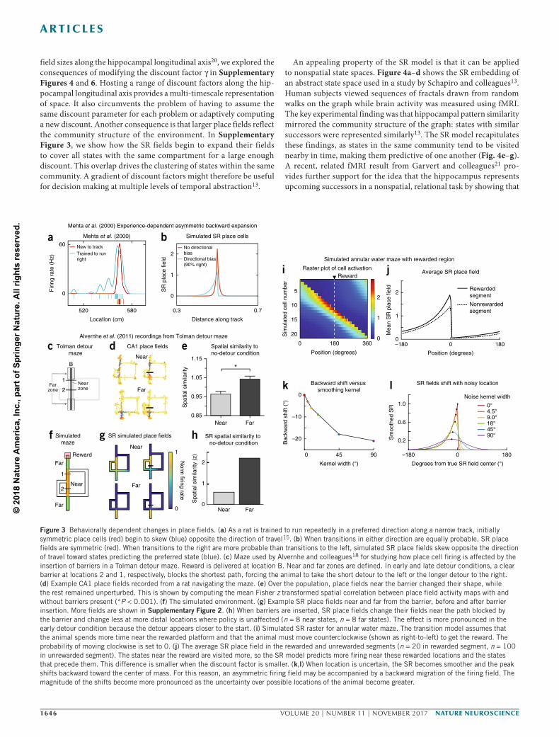
as states on opposite sides of a barrier cannot occur nearby in time. On the one-dimensional track, the SR place fields skew opposite the direction of travel (Fig. 2a–c). This backward skewing arises because upcoming states can be reliably predicted further in advance when traveling repeatedly in a particular direction. Neither of the control models provides a way for a directed behavioral policy to interact with state representation, and therefore they cannot show this effect. Evidence for predictive skewing comes from experiments in which animals traveled repeatedly in a particular direction along a linear track (Fig. 3)15. The authors noted this as evidence for predictive cod-ing in hippocampus15. In Figure 2d,e, we demonstrate how a future-oriented representation evokes a forward-skewing representation in the population at any given point in time but how such representa-tion implies that receptive fields for any individual cell should skew backwards. For a given cell to fire predictively, it must begin firing before its encoded state is visited, causing a backward-skewed recep-tive field. Figure 3a,b compares the predicted and experimentally observed backward skewing, demonstrating that the model captures the qualitative pattern of skewing observed when the animal has a directional bias.

Consistent with the SR and geodesic models, experiments have shown that place fields become distorted around barriers16–18. As shown in Figure 3c–h, we explored the effect on the SR place fields of placing obstacles in a Tolman detour maze and compared them to experimental results obtained by Alvernhe et al.18. When a barrier was placed in a maze such that the animal was forced to take a detour, the place fields engaged in local remapping. Place fields near the barrier changed their firing fields significantly more than those further from the barrier (P < 0.001; Fig. 3c–e). When barriers were inserted, SR place fields change more near the path blocked by the barrier and changed less at more distal locations where the optimal policy was unaffected (Fig. 3f–h). This locality is imposed by the discount factor. The full set of place fields is included Supplementary Figure 2.

The SR model can be used to explain how hippocampal place fields depend on behaviorally relevant features that alter an animal’s transi-tion policy, such as reward. Using an annular water maze, Hollup and colleagues demonstrated that a hidden, stationary reward affects the distribution of place fields19. Animals were required to swim in some preferred direction around a ring-shaped maze filled with an opaque liquid until they reached a hidden platform where they could rest. Hollup and colleagues found that the segment containing the plat-form had more place fields centered within it than any other segment and that the preceding segment consistently had the second-largest number of place fields centered within it.

We simulated this task using a sequence of states connected in a ring. The transition policy was such that the animal lingered longer near the rewarded location and had a preferred direction of travel, matching behavioral predictions recorded by the authors19. To simu-late this, we set the probability of transitioning in the antipreferred direction to 0 and increased the stay probability near the reward. As we show in Figure 3i–j, the SR model predicts elevated firing near the rewarded location and backward skewing of place fields. This creates an asymmetry, whereby the locations preceding the rewarded location also experience slightly higher firing rates. Furthermore, this asymmetric backward skew makes it likely that fields will overlap with the previous segment, not the upcoming segment. Figure 3c,d demonstrates how this backward skewing can equate to a backward shift in cell peak in the presence of noise or location uncertainty. This may explain the asymmetry found in the distribution of place field peaks around the rewarded segment.

While Hollup and colleagues found an asymmetric distribution of place cells about the rewarded segment, they also found that place fields were roughly the same size at reward locations as at other loca-tions. In contrast, the SR predicts that fields should get larger near reward locations (Fig. 3b), with the magnitude of this effect modu-lated by the discount factor (Supplementary Figs. 3–5). Thus, the SR is still an incomplete account of reward-dependent place fields.

Note that the SR model does not predict that place fields would be immediately affected by or dependent on the introduction of a reward. Rather, the shape of the fields should change as the animal gradually adjusts its policy and experiences multiple transitions con-sistent with that policy.

In addition to the influence of experimental factors, changes in parameters of the model will have systematic effects on the structure of SR place fields. Motivated by data showing a gradient of increasing

s2 s3 s4 s5

d Successor representation of states

e SR place field

s1 s2 s3 s4

s1 s2sss

Distance

0

1

0 1

a EuclideanGaussian

0

Successorrepresentation

Distance

0

1

0 1Distance

0

1

0 1Distance

0

1

0 1

Distance

0

1

0 1Distance

0

1

0 1

Tra

ck (

1D)

Firi

ng r

ate

(nor

m)

b c

1

Bar

rier

(2D

)D

ista

nce

Firing rate

M(s

1 , si )

M(s

5 , si )

M(s

j , s5 )

Goal

Goal

Goal

Geodesic

Figure 2 SR illustration and model comparison. (a–c) Top: One-dimensional track with left-to-right preferred direction of travel; red line marks the field center. Bottom: 2D environment with a barrier, indicated by gray line. (a) Euclidean Gaussian place field. Firing of place cells decays with Euclidean distance from the center of the field regardless of experience and environmental topology. (b) Geodesic Gaussian place field. Firing rate decays with geodesic distance from the center of the field, which respects boundaries in the environment but is invariant to the direction of travel11. (c) SR place field. Firing rate is proportional to the discounted expected number of visits to other states under the current policy (equation (3)). On the directed track, fields will skew opposite the direction of motion to anticipate the upcoming successor state. As the policy will not permit traversing walls, successor fields warp around obstacles. (d) Each colored column represents the firing rate M(s,s ) of a different place field located along the track, and the population vectors M(s1,:) and M(s5,:) illustrated here correspond to rows of the SR matrix. (e) The place field for a single SR-encoding cell skews backward toward past states that predict the cell’s preferred state. The receptive field M(:,s5) illustrated here corresponds to a column of the SR matrix.

© 2

018

Nat

ure

Am

eric

a, In

c., p

art o

f Spr

inge

r Nat

ure.

All

right

s re

serv

ed.

1646 VOLUME 20 | NUMBER 11 | NOVEMBER 2017 NATURE NEUROSCIENCE

A R T I C L E S

field sizes along the hippocampal longitudinal axis20, we explored the consequences of modifying the discount factor in Supplementary Figures 4 and 6. Hosting a range of discount factors along the hip-pocampal longitudinal axis provides a multi-timescale representation of space. It also circumvents the problem of having to assume the same discount parameter for each problem or adaptively computing a new discount. Another consequence is that larger place fields reflect the community structure of the environment. In Supplementary Figure 3, we show how the SR fields begin to expand their fields to cover all states with the same compartment for a large enough discount. This overlap drives the clustering of states within the same community. A gradient of discount factors might therefore be useful for decision making at multiple levels of temporal abstraction13.

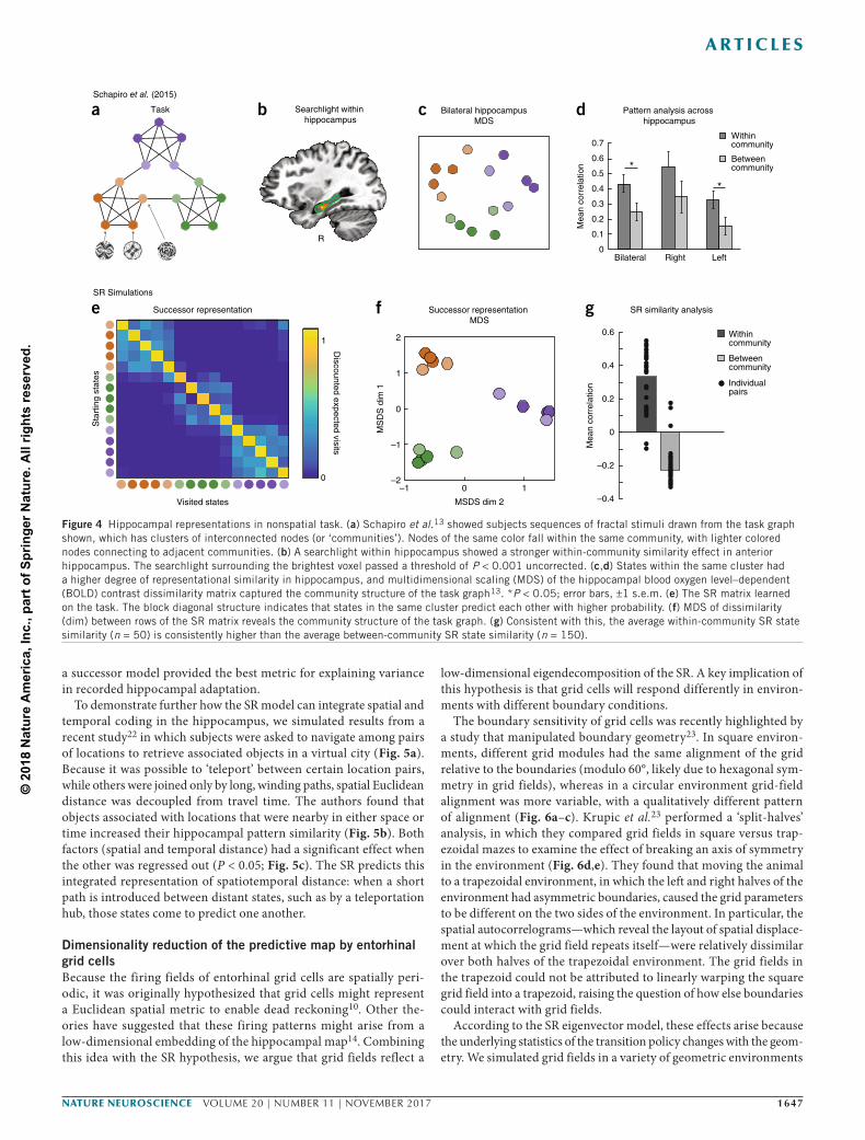
An appealing property of the SR model is that it can be applied to nonspatial state spaces. Figure 4a–d shows the SR embedding of an abstract state space used in a study by Schapiro and colleagues13. Human subjects viewed sequences of fractals drawn from random walks on the graph while brain activity was measured using fMRI. The key experimental finding was that hippocampal pattern similarity mirrored the community structure of the graph: states with similar successors were represented similarly13. The SR model recapitulates these findings, as states in the same community tend to be visited nearby in time, making them predictive of one another (Fig. 4e–g). A recent, related fMRI result from Garvert and colleagues21 pro-vides further support for the idea that the hippocampus represents upcoming successors in a nonspatial, relational task by showing that

0

1

0.3 0.7

0

1

2

SR

pla

ce fi

eld

Distance along track

Mehta et al. (2000)60

0

520

Location (cm)

580

Firi

ng r

ate

(Hz)

Simulated SR place cellsa bNo directionalbiasDirectional bias(90% right)

New to trackTrained to run right

0.2

0.6

1.0 0°4.5°9.0°18°45°90°

0 180–180

–20

–10

0

0 45 90

Bac

kwar

d sh

ift (

°)

Kernel width (°) Degrees from true SR field center (°)

Sm

ooth

ed S

RBackward shift versus

smoothing kernelSR fields shift with noisy location

Noise kernel width

5

10

1

2

0 360180

15

200 0

1

2

–180 1800

Raster plot of cell activationAverage SR place field

Position (degrees) Position (degrees)

Rewarded segment

Nonrewarded segment

Sim

ulat

ed c

ell n

umbe

r

i j

Mea

n S

R p

lace

fiel

dlk

Reward

0

1

2

Near Far

Spa

tial s

imila

rity

(z)

cAlvernhe et al. (2011) recordings from Tolman detour maze

Mehta et al. (2000) Experience-dependent asymmetric backward expansion

f

Far

Far

Near

Reward

2

1

Far

Near

*

Nearzone

Farzone

Spatial similarity to no-detour condition

CA1 place fields

Far

Near

SR spatial similarity to no-detour condition

SR simulated place fields

Norm

firing rate

d

g

e

h

Tolman detour maze

B

Simulatedmaze

1

2

Spa

tial s

imila

rity

Near Far

1.15

1.05

0.95

0.85

Simulated annular water maze with rewarded region

Figure 3 Behaviorally dependent changes in place fields. (a) As a rat is trained to run repeatedly in a preferred direction along a narrow track, initially symmetric place cells (red) begin to skew (blue) opposite the direction of travel15. (b) When transitions in either direction are equally probable, SR place fields are symmetric (red). When transitions to the right are more probable than transitions to the left, simulated SR place fields skew opposite the direction of travel toward states predicting the preferred state (blue). (c) Maze used by Alvernhe and colleagues18 for studying how place cell firing is affected by the insertion of barriers in a Tolman detour maze. Reward is delivered at location B. Near and far zones are defined. In early and late detour conditions, a clear barrier at locations 2 and 1, respectively, blocks the shortest path, forcing the animal to take the short detour to the left or the longer detour to the right. (d) Example CA1 place fields recorded from a rat navigating the maze. (e) Over the population, place fields near the barrier changed their shape, while the rest remained unperturbed. This is shown by computing the mean Fisher z transformed spatial correlation between place field activity maps with and without barriers present (*P < 0.001). (f) The simulated environment. (g) Example SR place fields near and far from the barrier, before and after barrier insertion. More fields are shown in Supplementary Figure 2. (h) When barriers are inserted, SR place fields change their fields near the path blocked by the barrier and change less at more distal locations where policy is unaffected (n = 8 near states, n = 8 far states). The effect is more pronounced in the early detour condition because the detour appears closer to the start. (i) Simulated SR raster for annular water maze. The transition model assumes that the animal spends more time near the rewarded platform and that the animal must move counterclockwise (shown as right-to-left) to get the reward. The probability of moving clockwise is set to 0. (j) The average SR place field in the rewarded and unrewarded segments (n = 20 in rewarded segment, n = 100 in unrewarded segment). The states near the reward are visited more, so the SR model predicts more firing near these rewarded locations and the states that precede them. This difference is smaller when the discount factor is smaller. (k,l) When location is uncertain, the SR becomes smoother and the peak shifts backward toward the center of mass. For this reason, an asymmetric firing field may be accompanied by a backward migration of the firing field. The magnitude of the shifts become more pronounced as the uncertainty over possible locations of the animal become greater.

© 2

018

Nat

ure

Am

eric

a, In

c., p

art o

f Spr

inge

r Nat

ure.

All

right

s re

serv

ed.

NATURE NEUROSCIENCE VOLUME 20 | NUMBER 11 | NOVEMBER 2017 1647

A R T I C L E S

a successor model provided the best metric for explaining variance in recorded hippocampal adaptation.

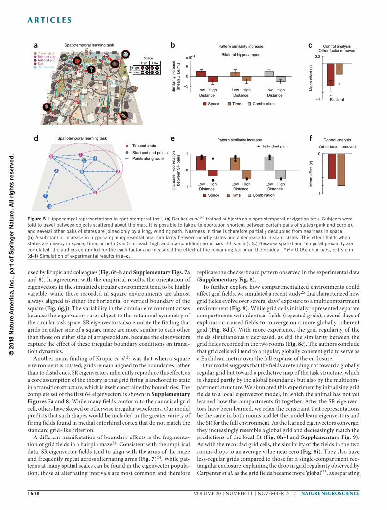
To demonstrate further how the SR model can integrate spatial and temporal coding in the hippocampus, we simulated results from a recent study22 in which subjects were asked to navigate among pairs of locations to retrieve associated objects in a virtual city (Fig. 5a). Because it was possible to ‘teleport’ between certain location pairs, while others were joined only by long, winding paths, spatial Euclidean distance was decoupled from travel time. The authors found that objects associated with locations that were nearby in either space or time increased their hippocampal pattern similarity (Fig. 5b). Both factors (spatial and temporal distance) had a significant effect when the other was regressed out (P < 0.05; Fig. 5c). The SR predicts this integrated representation of spatiotemporal distance: when a short path is introduced between distant states, such as by a teleportation hub, those states come to predict one another.

Dimensionality reduction of the predictive map by entorhinal grid cellsBecause the firing fields of entorhinal grid cells are spatially peri-odic, it was originally hypothesized that grid cells might represent a Euclidean spatial metric to enable dead reckoning10. Other the-ories have suggested that these firing patterns might arise from a low-dimensional embedding of the hippocampal map14. Combining this idea with the SR hypothesis, we argue that grid fields reflect a

low-dimensional eigendecomposition of the SR. A key implication of this hypothesis is that grid cells will respond differently in environ-ments with different boundary conditions.

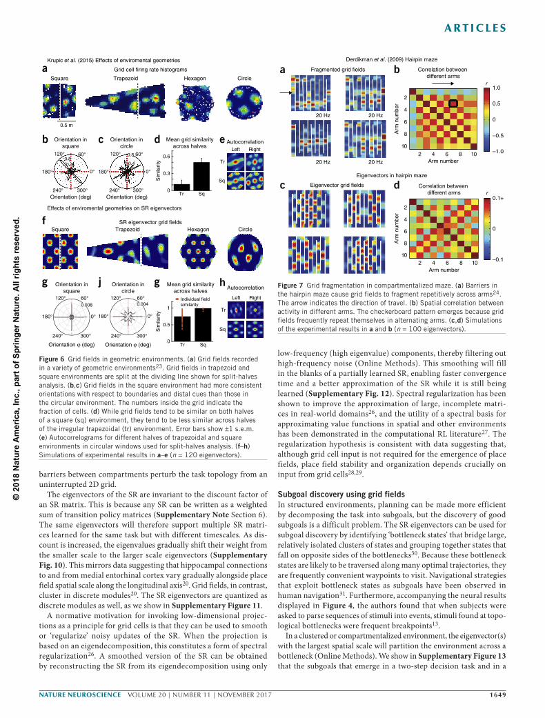
The boundary sensitivity of grid cells was recently highlighted by a study that manipulated boundary geometry23. In square environ-ments, different grid modules had the same alignment of the grid relative to the boundaries (modulo 60°, likely due to hexagonal sym-metry in grid fields), whereas in a circular environment grid-field alignment was more variable, with a qualitatively different pattern of alignment (Fig. 6a–c). Krupic et al.23 performed a ‘split-halves’ analysis, in which they compared grid fields in square versus trap-ezoidal mazes to examine the effect of breaking an axis of symmetry in the environment (Fig. 6d,e). They found that moving the animal to a trapezoidal environment, in which the left and right halves of the environment had asymmetric boundaries, caused the grid parameters to be different on the two sides of the environment. In particular, the spatial autocorrelograms—which reveal the layout of spatial displace-ment at which the grid field repeats itself—were relatively dissimilar over both halves of the trapezoidal environment. The grid fields in the trapezoid could not be attributed to linearly warping the square grid field into a trapezoid, raising the question of how else boundaries could interact with grid fields.

According to the SR eigenvector model, these effects arise because the underlying statistics of the transition policy changes with the geom-etry. We simulated grid fields in a variety of geometric environments

Bilateral hippocampusMDS

R

Searchlight within hippocampus

Pattern analysis across hippocampus

Withincommunity

Betweencommunity

Bilateral Right Left0

0.1

0.2

0.3

0.4

0.5

0.6

0.7

Mea

n co

rrel

atio

n

Task

Successor representation MDS

0

1

Sta

rtin

g st

ates

Visited states

Successor representation

SR Simulations

Schapiro et al. (2015)

a

eWithincommunity

Betweencommunity

Individualpairs

SR similarity analysis

b

f

dc

g

–1 0 1

MSDS dim 2

2

1

0

–1

–2

MS

DS

dim

1

–0.4

–0.2

0

0.2

0.4

0.6

Mea

n co

rrel

atio

n

*

*

Discounted expected visits

Figure 4 Hippocampal representations in nonspatial task. (a) Schapiro et al.13 showed subjects sequences of fractal stimuli drawn from the task graph shown, which has clusters of interconnected nodes (or ‘communities’). Nodes of the same color fall within the same community, with lighter colored nodes connecting to adjacent communities. (b) A searchlight within hippocampus showed a stronger within-community similarity effect in anterior hippocampus. The searchlight surrounding the brightest voxel passed a threshold of P < 0.001 uncorrected. (c,d) States within the same cluster had a higher degree of representational similarity in hippocampus, and multidimensional scaling (MDS) of the hippocampal blood oxygen level–dependent (BOLD) contrast dissimilarity matrix captured the community structure of the task graph13. *P < 0.05; error bars, 1 s.e.m. (e) The SR matrix learned on the task. The block diagonal structure indicates that states in the same cluster predict each other with higher probability. (f) MDS of dissimilarity (dim) between rows of the SR matrix reveals the community structure of the task graph. (g) Consistent with this, the average within-community SR state similarity (n = 50) is consistently higher than the average between-community SR state similarity (n = 150).

© 2

018

Nat

ure

Am

eric

a, In

c., p

art o

f Spr

inge

r Nat

ure.

All

right

s re

serv

ed.

1648 VOLUME 20 | NUMBER 11 | NOVEMBER 2017 NATURE NEUROSCIENCE

A R T I C L E S

used by Krupic and colleagues (Fig. 6f–h and Supplementary Figs. 7a and 8). In agreement with the empirical results, the orientation of eigenvectors in the simulated circular environment tend to be highly variable, while those recorded in square environments are almost always aligned to either the horizontal or vertical boundary of the square (Fig. 6g,j). The variability in the circular environment arises because the eigenvectors are subject to the rotational symmetry of the circular task space. SR eigenvectors also emulate the finding that grids on either side of a square maze are more similar to each other than those on either side of a trapezoid are, because the eigenvectors capture the effect of these irregular boundary conditions on transi-tion dynamics.

Another main finding of Krupic et al.23 was that when a square environment is rotated, grids remain aligned to the boundaries rather than to distal cues. SR eigenvectors inherently reproduce this effect, as a core assumption of the theory is that grid firing is anchored to state in a transition structure, which is itself constrained by boundaries. The complete set of the first 64 eigenvectors is shown in Supplementary Figures 7a and 8. While many fields conform to the canonical grid cell, others have skewed or otherwise irregular waveforms. Our model predicts that such shapes would be included in the greater variety of firing fields found in medial entorhinal cortex that do not match the standard grid-like criterion.

A different manifestation of boundary effects is the fragmenta-tion of grid fields in a hairpin maze24. Consistent with the empirical data, SR eigenvector fields tend to align with the arms of the maze and frequently repeat across alternating arms (Fig. 7)24. While pat-terns at many spatial scales can be found in the eigenvector popula-tion, those at alternating intervals are most common and therefore

replicate the checkerboard pattern observed in the experimental data (Supplementary Fig. 8).

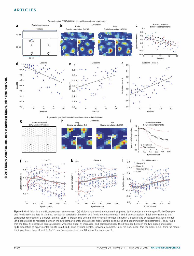
To further explore how compartmentalized environments could affect grid fields, we simulated a recent study25 that characterized how grid fields evolve over several days’ exposure to a multicompartment environment (Fig. 8). While grid cells initially represented separate compartments with identical fields (repeated grids), several days of exploration caused fields to converge on a more globally coherent grid (Fig. 8d,f). With more experience, the grid regularity of the fields simultaneously decreased, as did the similarity between the grid fields recorded in the two rooms (Fig. 8c). The authors conclude that grid cells will tend to a regular, globally coherent grid to serve as a Euclidean metric over the full expanse of the enclosure.

Our model suggests that the fields are tending not toward a globally regular grid but toward a predictive map of the task structure, which is shaped partly by the global boundaries but also by the multicom-partment structure. We simulated this experiment by initializing grid fields to a local eigenvector model, in which the animal has not yet learned how the compartments fit together. After the SR eigenvec-tors have been learned, we relax the constraint that representations be the same in both rooms and let the model learn eigenvectors and the SR for the full environment. As the learned eigenvectors converge, they increasingly resemble a global grid and decreasingly match the predictions of the local fit (Fig. 8h–l and Supplementary Fig. 9). As with the recorded grid cells, the similarity of the fields in the two rooms drops to an average value near zero (Fig. 8i). They also have less-regular grids compared to those for a single-compartment rec-tangular enclosure, explaining the drop in grid regularity observed by Carpenter et al. as the grid fields became more ‘global’25, as separating

0

1

×10–4

5

0.2

–1

Sim

ilarit

y in

crea

se(m

ean

± s.

e.m

.)

Mea

n ef

fect

(z)

0

–5

–1HighLow

Distance

HighLowDistance

HighLowDistance

HighLowDistance

HighHigh

Low

Low

Space

Space

Tim

e

Time Combination

Space Time Combination

HighLowDistance

HighLowDistanceIn

crea

se in

cor

rela

tion

betw

een

SR

pai

rs

Individual pair

Spatiotemporal learning task

–1

0

Control analysisOther factor removed

a b c

Pattern similarity increase

Pattern similarity increase

Bilateral hippocampus

Bilateral*

*

Spatiotemporal learning task Control analysis

Other factor removed

d e fTeleport ends

Teleport endBoxRoute/cone

9

2

81

132

15

12 33 4

1

14

10

311

7

2 25

1 6

Teleport startPlayer start

Start and end pointsPoints along route

Mea

n ef

fect

(z)

1

2 3

45

6

78

9

10

Figure 5 Hippocampal representations in spatiotemporal task. (a) Deuker et al.22 trained subjects on a spatiotemporal navigation task. Subjects were told to travel between objects scattered about the map. It is possible to take a teleportation shortcut between certain pairs of states (pink and purple), and several other pairs of states are joined only by a long, winding path. Nearness in time is therefore partially decoupled from nearness in space. (b) A substantial increase in hippocampal representational similarity between nearby states and a decrease for distant states. This effect holds when states are nearby in space, time, or both (n = 5 for each high and low condition; error bars, 1 s.e.m.). (c) Because spatial and temporal proximity are correlated, the authors controlled for the each factor and measured the effect of the remaining factor on the residual. *P < 0.05; error bars, 1 s.e.m. (d–f) Simulation of experimental results in a–c.

© 2

018

Nat

ure

Am

eric

a, In

c., p

art o

f Spr

inge

r Nat

ure.

All

right

s re

serv

ed.

NATURE NEUROSCIENCE VOLUME 20 | NUMBER 11 | NOVEMBER 2017 1649

A R T I C L E S

barriers between compartments perturb the task topology from an uninterrupted 2D grid.

The eigenvectors of the SR are invariant to the discount factor of an SR matrix. This is because any SR can be written as a weighted sum of transition policy matrices (Supplementary Note Section 6). The same eigenvectors will therefore support multiple SR matri-ces learned for the same task but with different timescales. As dis-count is increased, the eigenvalues gradually shift their weight from the smaller scale to the larger scale eigenvectors (Supplementary Fig. 10). This mirrors data suggesting that hippocampal connections to and from medial entorhinal cortex vary gradually alongside place field spatial scale along the longitudinal axis20. Grid fields, in contrast, cluster in discrete modules20. The SR eigenvectors are quantized as discrete modules as well, as we show in Supplementary Figure 11.

A normative motivation for invoking low-dimensional projec-tions as a principle for grid cells is that they can be used to smooth or ‘regularize’ noisy updates of the SR. When the projection is based on an eigendecomposition, this constitutes a form of spectral regularization26. A smoothed version of the SR can be obtained by reconstructing the SR from its eigendecomposition using only

low-frequency (high eigenvalue) components, thereby filtering out high-frequency noise (Online Methods). This smoothing will fill in the blanks of a partially learned SR, enabling faster convergence time and a better approximation of the SR while it is still being learned (Supplementary Fig. 12). Spectral regularization has been shown to improve the approximation of large, incomplete matri-ces in real-world domains26, and the utility of a spectral basis for approximating value functions in spatial and other environments has been demonstrated in the computational RL literature27. The regularization hypothesis is consistent with data suggesting that, although grid cell input is not required for the emergence of place fields, place field stability and organization depends crucially on input from grid cells28,29.

Subgoal discovery using grid fieldsIn structured environments, planning can be made more efficient by decomposing the task into subgoals, but the discovery of good subgoals is a difficult problem. The SR eigenvectors can be used for subgoal discovery by identifying ‘bottleneck states’ that bridge large, relatively isolated clusters of states and grouping together states that fall on opposite sides of the bottlenecks30. Because these bottleneck states are likely to be traversed along many optimal trajectories, they are frequently convenient waypoints to visit. Navigational strategies that exploit bottleneck states as subgoals have been observed in human navigation31. Furthermore, accompanying the neural results displayed in Figure 4, the authors found that when subjects were asked to parse sequences of stimuli into events, stimuli found at topo-logical bottlenecks were frequent breakpoints13.

In a clustered or compartmentalized environment, the eigenvector(s) with the largest spatial scale will partition the environment across a bottleneck (Online Methods). We show in Supplementary Figure 13 that the subgoals that emerge in a two-step decision task and in a

et al.

a

f

dc e

g j g h

b

Figure 6 Grid fields in geometric environments. (a) Grid fields recorded in a variety of geometric environments23. Grid fields in trapezoid and square environments are split at the dividing line shown for split-halves analysis. (b,c) Grid fields in the square environment had more consistent orientations with respect to boundaries and distal cues than those in the circular environment. The numbers inside the grid indicate the fraction of cells. (d) While grid fields tend to be similar on both halves of a square (sq) environment, they tend to be less similar across halves of the irregular trapezoidal (tr) environment. Error bars show 1 s.e.m. (e) Autocorrelograms for different halves of trapezoidal and square environments in circular windows used for split-halves analysis. (f–h) Simulations of experimental results in a–e (n = 120 eigenvectors).

et al

cr

d

ar

b

Figure 7 Grid fragmentation in compartmentalized maze. (a) Barriers in the hairpin maze cause grid fields to fragment repetitively across arms24. The arrow indicates the direction of travel. (b) Spatial correlation between activity in different arms. The checkerboard pattern emerges because grid fields frequently repeat themselves in alternating arms. (c,d) Simulations of the experimental results in a and b (n = 100 eigenvectors).

© 2

018

Nat

ure

Am

eric

a, In

c., p

art o

f Spr

inge

r Nat

ure.

All

right

s re

serv

ed.

1650 VOLUME 20 | NUMBER 11 | NOVEMBER 2017 NATURE NEUROSCIENCE

A R T I C L E S

–0.8

0

Local fit Global fit Global fit – local fit

Early LateSpatial correlation: 0.6206 Spatial correlation: 0.5259

Spatial correlationbetween compartments

Spatial environment Grid fields

–0.4

0.4

0.8

1.2

–0.6

0.4

0.8

0.6

–0.4

–0.2

0

0.20.5

0.9

0.7

0.3

0.1

Epoch numberEpoch numberEpoch number

0 200 300 400 5001000 200 300 400 5001000 200 300 400 500100

Glo

bal c

orre

latio

n fit

Loca

l cor

rela

tion

fit

Glo

bal f

it –

loca

l fit

0.2

0.4

0.6

0.8

1

0

0 200 300 400 500100

Mea

n sp

atia

l cor

rela

tion

Epoch number

Local fit Global fit Global fit – local fit

Spatial correlationbetween compartments

Early LateSpatial correlation: 1.0 Spatial correlation: 0.8701

Grid fields

Carpenter et al. (2015) Grid fields in multicompartment environment

a

Eigenvector grid fields learned in multicompartment environment

b c

d e f

h i

j k l

Standard errorMean corr

Standard error

Sample fitMean fit

LoBF

Discretized spatial simulation environment

g

A B

180 cm

40 cm

90 cm

10 cm

90 cm

A B

1

0.8

0.6

0.4

0.2

0

–0.2

–0.40 5 10 15 20

Session

1

0.9

0.8

0.7

0.6

0.5

0.4

0.3

0.20 5 10 15 20

Session Session Session0 5 10 15 20 0 5 10 15 20

1

0.9

0.8

0.7

0.6

0.5

0.4

0.3

0.2

0.6

0.4

0.2

0

–0.2

–0.4

–0.6

–0.8

Glo

bal f

it –

loca

l fit

Glo

bal f

it

Loca

l fit

Spa

tial c

orre

latio

n

Figure 8 Grid fields in a multicompartment environment. (a) Multicompartment environment employed by Carpenter and colleagues25. (b) Example grid fields early and late in training. (c) Spatial correlation between grid fields in compartments A and B across sessions. Each color refers to the correlation recorded for a different animal. (d,f) To explain this decline in intercompartmental similarity, Carpenter and colleagues fit a local model (grid constrained to replicate between the two compartments) and a global model (single continuous grid spanning both compartments). They found that the local fit decreased across sessions, while the global fit increased, and correspondingly, the difference between the two models increased. (g–l) Simulation of experimental results in a–f. (i–k) Blue or black circles, individual samples; thick red line, mean; thin red lines, 1 s.d. from the mean; thick gray lines, lines of best fit (loBF; n = 64 eigenvectors, n = 10 shown for each epoch).

© 2

018

Nat

ure

Am

eric

a, In

c., p

art o

f Spr

inge

r Nat

ure.

All

right

s re

serv

ed.

NATURE NEUROSCIENCE VOLUME 20 | NUMBER 11 | NOVEMBER 2017 1651

A R T I C L E S

multicompartment environment tend to fall near doorways and decision points: natural subgoals for high-level planning. The SR matrices parameterized by larger discount factors will project predomi-nantly on the large-spatial-scale grid components (Supplementary Fig. 10). The relationship between more temporally diffuse, abstract SRs, in which states in the same room are all encoded similarly (Supplementary Fig. 6), and the subgoals that join those clusters can therefore be captured by different eigenvalue thresholds.

It has been shown experimentally that entorhinal lesions impair performance on navigation tasks and disrupt the temporal ordering of sequential activations in hippocampus, while leaving performance on location-recognition tasks intact29,32. This suggests a role for grid cells in spatial planning and encourages us to speculate about a more general role for grid cells in hierarchical planning.

DISCUSSIONThe hippocampus has long been thought to encode a cognitive map, but the precise nature of this map is elusive. The traditional view, that the map is essentially spatial5, is not sufficient to explain some of the most striking aspects of hippocampal representation, such as the dependence of place fields on an animal’s behavioral policy and the environment’s topology. We argue instead that the map is essen-tially predictive, encoding expectations about an animal’s future state. This view resonates with earlier ideas about the predictive function of the hippocampus7,15,33–36. Our main contribution is a formaliza-tion of this predictive function in a reinforcement-learning frame-work, offering a new perspective on how the hippocampus supports adaptive behavior.

Our theory is connected to earlier work by Gustafson and Daw9 that showed how topologically sensitive spatial representations reca-pitulate many aspects of place cells and grid cells that are difficult to reconcile with a purely Euclidean representation of space. They also showed how encoding topological structure greatly aids rein-forcement learning in complex spatial environments. Earlier work by Foster and colleagues8 also used place cells as features for RL, although the spatial representation did not explicitly encode topologi-cal structure. While these theoretical precedents highlight the impor-tance of spatial representation, they leave open the deeper question of why particular representations are better than others. We showed that the SR naturally encodes topological structure in a format that enables efficient RL.

The work is also related to work by Dordek et al.14, who demon-strated grid-like activity patterns from principal components of the population activity of simulated Gaussian place cells. As we mentioned in the Results, one point of departure between empirically observed grid cell data and the SR eigenvector account is that, in rectangular environments, SR eigenvector grid fields can have different spatial scales aligned to the horizontal and vertical axis (Supplementary Fig. 7)10. In grid cells, the spatial scales tend to be approximately con-stant in all directions unless the environment changes37. However, Dordek et al. found that when the components were constrained to have non-negative values and the constraint that components be orthogonal was relaxed, the scaling became uniform in all direc-tions and the lattices became more hexagonal14. This suggests that the difference between SR eigenvectors and recorded grid cells is not fundamental to the idea that grid cells are doing spectral dimension-ality reduction. Rather, additional constraints such as non-negativity are required.

The SR can be viewed as occupying a middle ground between model-free and model-based learning12. Model-free learning requires storing a look-up table of cached values estimated from the

reward history1. By decomposing the value function into a predictive representation and a reward representation, the SR allows an agent to flexibly recompute values when rewards change, without sacrificing the computational efficiency of model-free methods4. Model-based learning is robust to changes in the reward structure, but it requires inefficient algorithms, like tree search, to compute values1.

Certain behaviors often attributed to a model-based system can be explained by any model in which the reward function is learned separately from predictions based on state dynamics. For instance, the ‘context pre-exposure facilitation effect’ refers to the finding that contextual fear conditioning is acquired more rapidly if the animal has the chance to explore the environment for several minutes before the first shock38. The facilitation effect is classically believed to arise from the development of a conjunctive representation of the context in the hippocampus, though areas outside the hippocampus may also develop a conjunctive representation in the absence of the hippoc-ampus, albeit less efficiently39. The SR provides a somewhat differ-ent interpretation: over the course of pre-exposure, the hippocampus develops a predictive representation of the context, such that subse-quent learning is rapidly propagated across space. Supplementary Figure 14 shows a simulation of this process and how it accounts for the facilitation effect.

Much prior work on prospective coding in the hippocampus has drawn inspiration from the well-documented ordered temporal struc-ture of firing in hippocampus relative to the theta phase7,40 and has considered the many ways in which replaying hippocampal sweeps dur-ing sharp wave-ripple events might support model-based, sequential forward planning41–43. The SR model, in contrast, is a predictive rate code, drawing its inspiration from the backward expansion of place cells that occur independently of sweeps and theta precession (see Supplementary Note Section 1 for more discussion)44,45.

The SR cannot replace the full functionality of model-based sweeps. However, it might provide a useful adjunct to the efficiency of this functionality. One way to combine the strengths of model-based planning with the SR would be to use the SR to extend the range of forward sweeps. In Supplementary Figure 15, we illustrate how per-forming sweeps in the successor representation space (Supplementary Fig. 15f,g) can extend the range of predictions, making the hippoc-ampal representations a more powerful substrate for planning. This is tantamount to a bootstrapped search algorithm46.

The SR model we describe is trained on the policy the animal has experienced. When the reward is changed, the new value function computed from the existing SR is initially based on the previous policy. The new optimal policy is unlikely to be the same as the old one, which means that the new value function must be refined as the animal optimizes its behavior. This is a tradeoff encountered with all learning algorithms that learn cached statistics under the current policy dynamics.

In some cases, the previous SR will be a reasonable initialization (Supplementary Fig. 15). Certain aspects of a task’s dynamics might not be subject to the animal’s control; notably, the underlying topol-ogy of the task. If new goals or subgoals are found in the vicinity of old goals, many policy components will generalize. It is hard to make com-prehensive claims about whether or not the space of naturalistic tasks adheres to these properties in general. However, recent computational work has demonstrated that deep successor features (a more powerful generalization of the successor representation model) generalize well across changing goals and environments in the domain of navigation47. Furthermore, the SR for a policy that supports more random explora-tion will naturally promote generalization. Spectral regularization can promote this by smoothing the SR over actions.

© 2

018

Nat

ure

Am

eric

a, In

c., p

art o

f Spr

inge

r Nat

ure.

All

right

s re

serv

ed.

1652 VOLUME 20 | NUMBER 11 | NOVEMBER 2017 NATURE NEUROSCIENCE

A R T I C L E S

When the SR fails to support value computation given the new reward, other mechanisms can compensate. Models such as Dyna update cached statistics using sweeps through a model, revising them flexibly46. The original form of Dyna demonstrated how model-based and model-free mechanisms could collaboratively update a value function. However, the value function can be replaced with any statistic learnable through temporal differences, including the SR, as demonstrated by recent work12. Furthermore, there is evidence from humans that when reward is changed, revaluation occurs in a policy-dependent manner, consistent with the kind of partial flex-ibility conferred by the SR48.

Recent work has elucidated connections between models of episodic memory and the SR. Specifically, Gershman et al. demonstrated that the SR is closely related to the temporal context model (TCM) of episodic memory11. The core idea of TCM is that items are bound to their tem-poral context (a running average of recently experienced items), and the currently active temporal context is used to cue retrieval of other items, which in turn cause their temporal context to be retrieved. The SR can be seen as encoding a set of item–context associations. The con-nection to episodic memory is especially interesting given the crucial mnemonic role played by the hippocampus and entorhinal cortex in episodic memory. Howard and colleagues49 have laid out a detailed mapping between TCM and the medial temporal lobe (including entorhinal and hippocampal regions).

Spectral graph theory provides insight into the topological struc-ture encoded by the SR. We showed specifically that eigenvectors of the SR can be used to discover a hierarchical decomposition of the environment for use in hierarchical RL. Spectral analysis has also fre-quently been invoked as a computational motivation for entorhinal grid cells (for example, Krupic, Burgess & O’Keefe50). The fact that any function can be reconstructed by sums of sinusoids suggests that the entorhinal cortex implements a kind of Fourier transform of space. However, Fourier analysis is not the right mathematical tool when dealing with spatial representations in a topologically structured envi-ronment (Supplementary Fig. 13b), as we do not expect functions to be smooth over boundaries in the environment. This is precisely the purpose of spectral graph theory: instead of being maximally smooth over Euclidean space, the eigenvectors of the SR (equivalently, the eigenvectors of the graph Laplacian) embed the smoothest approxima-tion of a function that respects the graph topology28 (Supplementary Note Sections 2–7).

In conclusion, the SR provides a unifying framework for a wide range of observations about the hippocampus and entorhinal cortex. The multifaceted functions of these brain regions can be understood as serving a superordinate goal of prediction.

METHODSMethods, including statements of data availability and any associated accession codes and references, are available in the online version of the paper.

Note: Any Supplementary Information and Source Data files are available in the online version of the paper.

ACKNOWLEDGMENTSWe are grateful to T. Behrens, I. Mommenejad, and K. Miller for helpful discussions, and to A. Mathis, H. Sanders, M. Chadwick, and D. Kumaran for comments on an earlier draft of the paper. This research was supported by the NSF Collaborative Research in Computational Neuroscience (CRCNS) Program Grant IIS-120 7833 and The John Templeton Foundation. The opinions expressed in this publication are those of the authors and do not necessarily reflect the views of the funding agencies.

AUTHOR CONTRIBUTIONSAll authors conceived the model and wrote the manuscript. Simulations were carried out by K.S.

COMPETING FINANCIAL INTERESTSThe authors declare no competing financial interests.

Reprints and permissions information is available online at http://www.nature.com/reprints/index.html. Publisher’s note: Springer Nature remains neutral with regard to jurisdictional claims in published maps and institutional affiliations.

1. Daw, N.D., Niv, Y. & Dayan, P. Uncertainty-based competition between prefrontal and dorsolateral striatal systems for behavioral control. Nat. Neurosci. 8, 1704–1711 (2005).

2. Tolman, E.C. Cognitive maps in rats and men. Psychol. Rev. 55, 189–208 (1948).

3. Schultz, W., Dayan, P. & Montague, P.R. A neural substrate of prediction and reward. Science 275, 1593–1599 (1997).

4. Dayan, P. Improving generalization for temporal difference learning: the successor representation. Neural Comput. 5, 613–624 (1993).

5. O’Keefe, J. & Nadel, L. The Hippocampus as a Cognitive Map (Clarendon Press, 1978).

6. Muller, R.U., Stead, M. & Pach, J. The hippocampus as a cognitive graph. J. Gen. Physiol. 107, 663–694 (1996).

7. Penny, W.D., Zeidman, P. & Burgess, N. Forward and backward inference in spatial cognition. PLOS Comput. Biol. 9, e1003383 (2013).

8. Foster, D.J., Morris, R.G. & Dayan, P. A model of hippocampally dependent navigation, using the temporal difference learning rule. Hippocampus 10, 1–16 (2000).

9. Gustafson, N.J. & Daw, N.D. Grid cells, place cells, and geodesic generalization for spatial reinforcement learning. PLOS Comput. Biol. 7, e1002235 (2011).

10. Hafting, T., Fyhn, M., Molden, S., Moser, M.B. & Moser, E.I. Microstructure of a spatial map in the entorhinal cortex. Nature 436, 801–806 (2005).

11. Gershman, S.J., Moore, C.D., Todd, M.T., Norman, K.A. & Sederberg, P.B. The successor representation and temporal context. Neural Comput. 24, 1553–1568 (2012).

12. Russek, E.M., Momennejad, I., Botvinick, M.M., Gershman, S.J. & Daw, N.D. Predictive representations can link model-based reinforcement learning to model-free mechanisms. Preprint at https://doi.org/10.1101/083857 (2017).

13. Schapiro, A.C., Turk-Browne, N.B., Norman, K.A. & Botvinick, M.M. Statistical learning of temporal community structure in the hippocampus. Hippocampus 26, 3–8 (2016).

14. Dordek, Y., Meir, R. & Derdikman, D. Extracting grid characteristics from spatially distributed place cell inputs using non-negative PCA. Preprint at https://arxiv.org/abs/1505.03711 (2015).

15. Mehta, M.R., Quirk, M.C. & Wilson, M.A. Experience-dependent asymmetric shape of hippocampal receptive fields. Neuron 25, 707–715 (2000).

16. Muller, R.U. & Kubie, J.L. The effects of changes in the environment on the spatial firing of hippocampal complex-spike cells. J. Neurosci. 7, 1951–1968 (1987).

17. Skaggs, W.E. & McNaughton, B.L. Spatial firing properties of hippocampal CA1 populations in an environment containing two visually identical regions. J. Neurosci. 18, 8455–8466 (1998).

18. Alvernhe, A., Save, E. & Poucet, B. Local remapping of place cell firing in the Tolman detour task. Eur. J. Neurosci. 33, 1696–1705 (2011).

19. Hollup, S.A., Molden, S., Donnett, J.G., Moser, M.B. & Moser, E.I. Accumulation of hippocampal place fields at the goal location in an annular water maze task. J. Neurosci. 21, 1635–1644 (2001).

20. Strange, B.A., Witter, M.P., Lein, E.S. & Moser, E.I. Functional organization of the hippocampal longitudinal axis. Nat. Rev. Neurosci. 15, 655–669 (2014).

21. Garvert, M.M., Dolan, R.J. & Behrens, T.E. A map of abstract relational knowledge in the human hippocampal-entorhinal cortex. eLife 6, 17086 (2017).

22. Deuker, L., Bellmund, J.L., Navarro Schröder, T. & Doeller, C.F. An event map of memory space in the hippocampus. eLife 5, e16534 (2016).

23. Krupic, J., Bauza, M., Burton, S., Barry, C. & O’Keefe, J. Grid cell symmetry is shaped by environmental geometry. Nature 518, 232–235 (2015).

24. Derdikman, D. et al. Fragmentation of grid cell maps in a multicompartment environment. Nat. Neurosci. 12, 1325–1332 (2009).

25. Carpenter, F., Manson, D., Jeffery, K., Burgess, N. & Barry, C. Grid cells form a global representation of connected environments. Curr. Biol. 25, 1176–1182 (2015).

26. Mazumder, R., Hastie, T. & Tibshirani, R. Spectral regularization algorithms for learning large incomplete matrices. J. Mach. Learn. Res. 11, 2287–2322 (2010).

27. Mahadevan, S. & Maggioni, M. Proto-value functions: a Laplacian framework for learning representation and control in markov decision processes. J. Mach. Learn. Res. 8, 2169–2231 (2007).

28. Bonnevie, T. et al. Grid cells require excitatory drive from the hippocampus. Nat. Neurosci. 16, 309–317 (2013).

29. Hales, J.B. et al. Medial entorhinal cortex lesions only partially disrupt hippocampal place cells and hippocampus-dependent place memory. Cell Rep. 9, 893–901 (2014).

30. Solway, A. et al. Optimal behavioral hierarchy. PLoS Comput. Biol. 10, e1003779 (2014).

31. Ribas-Fernandes, J.J. et al. A neural signature of hierarchical reinforcement learning. Neuron 71, 370–379 (2011).

© 2

018

Nat

ure

Am

eric

a, In

c., p

art o

f Spr

inge

r Nat

ure.

All

right

s re

serv

ed.

NATURE NEUROSCIENCE VOLUME 20 | NUMBER 11 | NOVEMBER 2017 1653

A R T I C L E S

32. Schlesiger, M.I. et al. The medial entorhinal cortex is necessary for temporal organization of hippocampal neuronal activity. Nat. Neurosci. 18, 1123–1132 (2015).

33. Blum, K.I. & Abbott, L.F. A model of spatial map formation in the hippocampus of the rat. Neural Comput. 8, 85–93 (1996).

34. Levy, W.B., Hocking, A.B. & Wu, X. Interpreting hippocampal function as recoding and forecasting. Neural Netw. 18, 1242–1264 (2005).

35. Hassabis, D. & Maguire, E.A. The construction system of the brain. Phil. Trans. R. Soc. Lond. B 364, 1263–1271 (2009).

36. Buckner, R.L. The role of the hippocampus in prediction and imagination. Annu. Rev. Psychol. 61, 27–48, C1–C8 (2010).

37. Barry, C., Hayman, R., Burgess, N. & Jeffery, K.J. Experience-dependent rescaling of entorhinal grids. Nat. Neurosci. 10, 682–684 (2007).

38. Fanselow, M.S. From contextual fear to a dynamic view of memory systems. Trends Cogn. Sci. 14, 7–15 (2010).

39. Wiltgen, B.J., Sanders, M.J., Anagnostaras, S.G., Sage, J.R. & Fanselow, M.S. Context fear learning in the absence of the hippocampus. J. Neurosci. 26, 5484–5491 (2006).

40. Maurer, A.P. & McNaughton, B.L. Network and intrinsic cellular mechanisms underlying theta phase precession of hippocampal neurons. Trends Neurosci. 30, 325–333 (2007).

41. Johnson, A. & Redish, A.D. Neural ensembles in CA3 transiently encode paths forward of the animal at a decision point. J. Neurosci. 27, 12176–12189 (2007).

42. Pezzulo, G., van der Meer, M.A., Lansink, C.S. & Pennartz, C.M. Internally generated sequences in learning and executing goal-directed behavior. Trends Cogn. Sci. 18, 647–657 (2014).

43. Hasselmo, M.E. & Stern, C.E. Theta rhythm and the encoding and retrieval of space and time. Neuroimage 85, 656–666 (2014).

44. Ekstrom, A.D., Meltzer, J., McNaughton, B.L. & Barnes, C.A. NMDA receptor antagonism blocks experience-dependent expansion of hippocampal “place fields”. Neuron 31, 631–638 (2001).

45. Hafting, T., Fyhn, M., Bonnevie, T., Moser, M.-B. & Moser, E.I. Hippocampus-independent phase precession in entorhinal grid cells. Nature 453, 1248–1252 (2008).

46. Sutton, R.S. DYNA, an integrated architecture for learning, planning, and reacting. ACM SIGART Bulletin 2, 160–163 (1991).

47. Zhang, J., Springenberg, J.T., Boedecker, J. & Burgard, W. Deep reinforcement learning with successor features for navigation across similar environments. IEEE/RSJ International Conference on Intelligent Robots and Systems (2017).

48. Momennejad, I. et al. The successor representation in human reinforcement learning. Preprint at https://doi.org/10.1101/083824 (2017).

49. Howard, M.W., Fotedar, M.S., Datey, A.V. & Hasselmo, M.E. The temporal context model in spatial navigation and relational learning: toward a common explanation of medial temporal lobe function across domains. Psychol. Rev. 112, 75–116 (2005).

50. Krupic, J., Burgess, N. & O’Keefe, J. Neural representations of location composed of spatially periodic bands. Science 337, 853–857 (2012).

© 2

018

Nat

ure

Am

eric

a, In

c., p

art o

f Spr

inge

r Nat

ure.

All

right

s re

serv

ed.

NATURE NEUROSCIENCE doi:10.1038/nn.4650

ONLINE METHODSThe reinforcement learning problem. We consider the problem of RL in a Markov decision process consisting of the following elements51: a set of states (for example, spatial locations), a set of actions, a transition distribution P(s |s,a) specifying the probability of transitioning to state s from state s after taking action a, a reward function R(s) specifying the expected immediate reward in state s, and a discount factor [0, 1] that downweights distal rewards. An agent chooses actions according to a policy (a|s) and collects rewards as it moves through the state space. The value of a state is defined formally as the expected discounted cumulative future reward under policy (same as equation (1), with dependence on included in notation here):

V s R s s st

tt( ) ( ) | ( )

00 4g

where st is the state visited at time t. Our focus here is on policy evaluation (computing V). In our simulations we feed the agent the optimal policy; in the Discussion we discuss algorithms for policy improvement. To simplify notation, we assume implicit dependence on and define the state transition matrix T, where

T s s a s P s s aa

( , ) ( | ) ( | , ) ( )p 5

Task simulation. Environments were simulated by discretizing the plane into points and connecting these points along a triangular lattice (Supplementary Fig. 17a). The adjacency matrix A was constructed such that A(s,s ) = 1 wherever it is possible to transition between states s and s and 0 otherwise. The effect of different discretizations is considered in Supplementary Note Section 8 and Supplementary Figure 18.

The transition probability matrix T was defined such that T(s,s ) is the prob-ability of transitioning from state s to s (equation (5)). Under a random walk policy, where the agent chooses randomly among all available transitions, the transition probability distribution is uniform over allowable transitions. This amounts to simply normalizing A so that each row of A sums to 1 to meet the constraint that all possible transitions from s must sum to 1. When reward or punishment was included as part of the simulated task, we computed the optimal policy using value iteration and a softmax value function parameterized by (ref. 51). Supplementary Note Section 8 and Supplementary Figure 4 consider the effect of manipulating the softmax parameter .

Parameters for all simulations are included in Supplementary Note Section 8.

SR computation. The successor representation is a matrix, M, where M(s,s ) is equal to the discounted expected number of times the agent visits state s start-ing from s (see equation (3) for the mathematical definition and Supplementary Fig. 17b for an illustration). When the transition probability matrix is known, we can compute the SR as a discounted sum over transition matrices raised to the exponent t. The matrix Tt is the t-step transition matrix, where Tt(s,s ) is the probability of transitioning from s to s in exactly t steps.

M Tt

t t

06g ( )

This sum is a geometric matrix series, and for < 1, it converges to the follow-ing finite analytical solution:

M T I Tt

t t

0

1 7g g( ) ( )

where I is the identity matrix. In most of our simulations, the SR was computed analytically from the transition matrix using this expression. The effects of manipulating the discount factor is discussed in Supplementary Note Section 8 and illustrated in Supplementary Figure 5.

The SR can be learned online using the temporal differences update rule shown below after each transition4 (also see ref. 51 for background on TD learning;

(4)(4)

(5)(5)

(6)(6)

(7)(7)

Fig. 8 and Supplementary Figs. 2, 10, and 13). After observing a transition st st + 1, the estimate is updated according to

ˆ ( ) ˆ ( ) ˆ ( ) ˆ ( ), , ( ) , ,M s s M s s s s M s s M s st t t t t t t t t1 1h g ( )8

where is a learning rate (unless specified otherwise, = 0.1 in our simulations). The form of this update is identical to the temporal difference learning rule for value functions51, except that in this case the reward prediction error is replaced by a successor prediction error (the term in brackets). Note that these prediction errors are distinct from state prediction errors used to update an estimate of the transition function52; the SR predicts not just the next state but a superposition of future states over a possibly infinite horizon. The transition and SR functions only coincide when = 0. We assume the SR matrix M is initialized to the identity matrix, meaning M(s,s ) = 1 if s = s , and M(s,s ) = 0 if s s . This initialization can be understood to mean that each state will necessarily predict only itself.

Eigenvector computation and spectral regularization. In generating the grid cells shown, we assume a random walk policy, which is the maximum entropy prior for policies (see ref. 53 for why maximum entropy priors can be good priors for regularization). However, as the learned eigenvectors are sensitive to the sam-pling statistics, our model predicts that regions of the task space more frequently visited would come to be over-represented in the grid space (see Supplementary Fig. 19 for examples). After computing the eigenvectors, we then threshold them at 0 so that firing rates are not negative (Supplementary Fig. 17d).

For Figure 8, eigenvectors were computed incrementally using candid covari-ance-free incremental PCA (CCIPCA), an algorithm that efficiently implements stochastic gradient descent to compute principal components54 (eigenvectors and principal components are approximately equivalent in this domain). Spectral regularization was implemented by reconstructing the SR from the truncated eigendecomposition (Supplementary Note Section 4 and Supplementary Fig. 12). Spectral reconstruction for Supplementary Figure 12 was implemented by shifting the eigenvalues to place more weight on low-frequency eigenvectors rather than imposing a hard cutoff on high-frequency eigenvectors and by recon-structing an SR that corresponded to a larger discount factor. This allowed larger-discount SRs to be more exactly approximated. The reconstructed SR matrices Mrecon were compared to the ground truth matrix Mgt by taking the correla-tion between Mrecon and Mgt (Supplementary Fig. 12). This measure indicates whether policies based on SR-based value functions for different reward functions will to tend send the animal in the right direction.

Subgoal partitioning with normalized min-cut. In Supplementary Figure 13, we show subgoals computed from the first k eigenvectors of the graph Laplacian. The formal problem of identifying bottlenecks in a graph to produce subgoals is known as the k-way normalized min-cut problem. An approximate solution can be obtained using spectral graph theory55. First, the top log k eigenvectors of a matrix known as the graph Laplacian are thresholded such that negative ele-ments of each eigenvector go to 0 and positive elements go to 1. Edges that travel between these two labeled groups of states are ‘cut’ by the partition, and nodes adjacent to these edges are a kind of bottleneck subgoal. The first subgoals that emerge will lie on the edges cut by the lowest-frequency eigenvector, and these subgoals will approximately lie between the two largest, most separable clusters in the partition (see Supplementary Note Section 5 for more detail). A prioritized sequence of subgoals is obtained by incorporating increasingly higher frequency eigenvectors that produce partition points nearer to the agent. The SR shares its eigenvectors with the graph Laplacian (Supplementary Note Section 5), making SR eigenvectors equally suitable for this process of subgoal discovery.

Plotting receptive fields. To visualize place fields under the SR model, we cre-ated heat maps of how active each SR-encoding neuron would be at each state in the environment (Supplementary Fig. 17e,f). These maps show the discounted expected number of times the neuron’s encoded state s will be visited from each other state in the environment and correspond to taking a column M(s,:) from the SR matrix and reshaping it so that each element appears at the x,y location of its corresponding state. We use the same reshaping and plotting procedure to visualize eigenvector grid cells, using the columns of the thresholded eigenvector matrix U in place of M.

(8)(8)

© 2

018

Nat

ure

Am

eric

a, In

c., p

art o

f Spr

inge

r Nat

ure.

All

right

s re

serv

ed.

NATURE NEUROSCIENCEdoi:10.1038/nn.4650

Statistics. In Figure 8, spatial similarity was computed by taking the Fisher z transform of spatial correlation between fields. Statistics shown (mean, s.d.) were computed in this z space.

Grid field quantifications paralleled the analyses of Krupic et al.23: an ellipse was fit to the six peaks closest to the central peak, and ‘orientation’ refers to the orientation of the main axes (a,b). ‘Correlation’ always refers to the Pearson correlation, ‘spatial correlation’ refers to the Pearson correlation computed over points in space (as opposed to points in a vector), and spatial autocorrelation refers to the 2D autoconvolution.

To measure similarity between halves of the environment in Figure 6, we (i) computed the spatial autocorrelation for each half, (ii) selected a circular window in the center of the autocorrelation, and (iii) computed the correlation between autocorrelations of the two halves in the window. This paralleled the analysis per-formed by Krupic et al.23 and provides a measure of grid similarity across halves of the environment. The circular window is used to control for the fact that the boundaries of the square and trapezoid in the two halves of the respective envi-ronments differ. The mean similarity was not computed in Fisher z-transformed space, as one would normally do, but rather in correlation space. This was because the similarity for many of the square eigenvectors and at least one trapezoidal eigenvector was exactly 1, for which z = `. A dot plot is superimposed over this plot so the statistics of the distribution can be visualized.

In evaluating our simulations of the grid fields reported by Carpenter et al.25 (Fig. 8), the local model consisted of the set of 2D Fourier components bounded

by the size of the compartment, and the global model consisted of the set of 2D Fourier components bounded by the size of the environment. ‘Model fit’ was measured for each eigenvector by finding maximum correlation over all model components between the eigenvector and model component.

Code availability. These results were generated using code written in Matlab. Code is available at https://github.com/kstach01/predictive-hc.

Data avilablity. Data sharing is not applicable to this article as no datasets were generated or analyzed during the current study.

A Life Science Reporting Summary for this paper is available.

51. Sutton, R. & Barto, A. Reinforcement Learning: an Introduction (MIT Press, 1998).

52. Gläscher, J., Daw, N., Dayan, P. & O’Doherty, J.P. States versus rewards: dissociable neural prediction error signals underlying model-based and model-free reinforcement learning. Neuron 66, 585–595 (2010).

53. Bialek, W. Biophysics: Searching for Principles (Princeton University Press, 2012).

54. Weng, J., Zhang, Y. & Hwang, W. Candid covariance-free incremental principal component analysis. IEEE Trans. Pattern Anal. Mach. Intell. 25, 1034–1040 (2003).

55. Shi, J. & Malik, J. Normalized cuts and image segmentation. IEEE Trans. Pattern Anal. Mach. Intell. 22, 888–905 (2000).