THE HIGH TIME RESOLUTION

RADIO SKY

A THESIS SUBMITTED TO THE UNIVERSITY OF MANCHESTER FOR THE

DEGREE OF DOCTOR OF PHILOSOPHY IN THE FACULTY OF

ENGINEERING AND PHYSICAL SCIENCES

2013

BY

DAN PHILIP GRANT THORNTONSCHOOL OF PHYSICS AND ASTRONOMY

2

The University of ManchesterABSTRACT OF THESIS submitted by Dan Philip Grant Thornton

for the Degree of Doctor of Philosophy and entitled“The High Time Resolution Radio Sky”

September 2013

Pulsars are laboratories for extreme physics unachievable on Earth. As individualsources and possible orbital companions can be used to study magnetospheric, emission,and superfluid physics, general relativistic effects, and stellar and binary evolution. As pop-ulations they exhibit a wide range of sub-types, with parameters varying by many ordersof magnitude signifying fundamental differences in their evolutionary history and potentialuses. There are currently around 2200 known pulsars in the Milky Way, the Magellanicclouds, and globular clusters, most of which have been discovered with radio survey ob-servations. These observations, as well as being suitable for detecting the repeating signalsfrom pulsars, are well suited for identifying other transient astronomical radio bursts thatlast just a few milliseconds that either singular in nature, or rarely repeating.

Prior to the work of this thesis non-repeating radio transients at extragalactic distanceshad possibly been discovered, however with just one example status a real astronomicalsources was in doubt. Finding more of these sources was a vital to proving they were realand to open up the universe for millisecond-duration radio astronomy.

The High Time Resolution Universe survey uses the multibeam receiver on the 64-mParkes radio telescope to search the whole visible sky for pulsars and transients. The tem-poral and spectral resolution of the receiver and the digital back-end enable the detectionof relatively faint, and distant radio sources. From the Parkes telescope a large portion ofthe Galactic plane can be seen, a rich hunting ground for radio pulsars of all types, whilepreviously poorly surveyed regions away from the Galactic plane are also covered.

I have made a number of pulsar discoveries in the survey, including some rare systems.These include PSR J1226−6208, a possible double neutron star system in a remarkably cir-cular orbit, PSR J1431−471 which is being eclipsed by its companion with each orbit, PSRJ1729−2117 which is an unusual isolated recycled pulsar, and PSR J2322−2650 which hasa companion of very low mass − just 7× 10−4M, amongst others. I begin this thesis withthe study of these pulsars and discuss their histories. In addition, I demonstrate that opticalobservations of the companions to some of the newly discovered pulsars in the High TimeResolution Universe survey may result in a measurement of their age and that of the pulsar.

I have discovered five new extragalactic single radio bursts, confirming them as an astro-nomical population. These appear to occur frequently, with a rate of 1.0+0.6

−0.5×104 sky−1 day−1.The sources are likely at cosmological distances − with redshifts between 0.45 and 1.45,making them more than half way to the Big Bang in the most distant case. This impliestheir luminosities must be enormous, 1031 to 1033 J emitted in just a few milliseconds. Theirsource is unknown but I present an analysis of the options. I also perform a population sim-ulation of the bursts which demonstrates how their intrinsic spectrum could be measured,even for unlocalised FRBs: early indications are that the spectral index of FRBs < 0.

D P G THORNTON 3

Declaration

No portion of the work referred to in this thesis has been submitted in support of anapplication for another degree or qualification of this or any other university or other insti-tution of learning.

Dan Philip Grant ThorntonDepartment of Physics and Astronomy

University of ManchesterJodrell Bank Centre for Astrophysics

Alan Turing BuildingUniversity of Manchester

ManchesterM13 9PL

United Kingdom

4

Copyright

Copyright in text of this thesis rests with the Author. Copies (by any process) either infull, or of extracts, may be made only in accordance with instructions given by the Authorand lodged in the John Rylands University Library of Manchester. Details may be obtainedfrom the Librarian. This page must form part of any such copies made. Further copies (byany process) of copies made in accordance with such instructions may not be made withoutthe permission (in writing) of the Author. The ownership of any intellectual property rightswhich may be described in this thesis is vested in the University of Manchester, subjectto any prior agreement to the contrary, and may not be made available for use by thirdparties without the written permission of the University, which will prescribe the termsand conditions of any such agreement. Further information on the conditions under whichdisclosures and exploitation may take place is available from the head of Department ofPhysics and Astronomy.

D P G THORNTON 5

Acknowledgements

During my PhD I have been lucky enough to work with some outstanding scientists andmentors. Not least my supervisor Ben Stappers whose support over the three years has beenbrilliant. Your guidance and help has been invaluable, thanks for giving me the opportunityto work on such great projects.

In the course of my work I have also worked and interacted with some talented scien-tists at Jodrell Bank, in no particular order, Andrew Lyne, Sir Francis Graham-Smith, ChrisJordan, Cees Bassa, Gemma Janssen, Patrick Weltevrede, Rob Ferdman, Mike Keith, MarkPurver, Cristobal Espinoza, Evan Keane, Sam Bates, Tom Hassall, Neil Young, SotiriosSanidas, Kuo Liu, Phrudth Jaroenjittichai, Monika Obrocka, Rob Lyon, Sally Cooper, andSimon Rookyard. In differing proportions you’ve made the last three years funny, chal-lenging, interesting, and above all enjoyable. To Ant Holloway and Bob Dickson, this PhDwould have been next to impossible without your help and hard work.

The HITRUN collaboration, you gave me the opportunity to work on this excellentsurvey. Thanks to all of you, in particular Michael Kramer, Matthew Bailes, and SimonJohnston for helping me along the way. Thanks also to Andrea Possenti for showing methe ropes that first time at Parkes.

I have been lucky to spend several months observing with the Parkes radio telescope,where the staff and scientists have always looked after me, particularly John Sarkissian,a brilliant scientist who makes a visit to Parkes all the more interesting, and who doesn’tmind the 5 am phone calls. Of course no PhD which uses Parkes should fail to acknowledgeall the staff who work at the telescope - here’s to another 50 years of pulsars, FRBs, andanything else which may pop up! Thanks also to my friends at the ATNF who took me totrivia and made being so far from home bearable, Shari Breen and Ryan Shannon, and themultitude of friendly people down under.

To the people who have supported me for so long, mum and dad. You were right, doingthe hard subjects at school was the right thing to do! To Rosie and Miri, thanks for beingsuch great sisters.

And finally to my Lucy, without you this would never have been possible, thank youfor supporting me and being so patient with me. All those times when I said I couldn’t doit, you kept me going. This one’s for you. PB.

6

Acronyms

BPSR Berkeley-Parkes-Swinburne recorder

ccSN Core-collapse supernova

DFT Discrete Fourier transform

DM Dispersion measure

FFT Fast Fourier transform

FPGA Field programmable gate array

FRB Fast radio burst

(SH)GRB (Short hard) Gamma-ray burst

HPBW Half-power beam-width

HTRU High time resolution universe [survey]

H/LMXB High/Low mass x-ray binary

IGM Intergalactic medium

ISM Interstellar medium

JBO Jodrell Bank Observatory

MB Multibeam [receiver]

MSP Millisecond pulsar

MW Milky Way

NS Neutron star

DNS Double neutron star

PMPS Parkes multibeam pulsar survey

RFI Radio frequency interference

RRAT Rotating radio transient

SNR Signal to noise ratio

UTC Coordinated universal time

WD White dwarf

D P G THORNTON 7

Refereed publications

A population of fast radio bursts at cosmological distancesThornton D., et al.

2013Science, 341 6141 pp. 53 – 56

The High Time Resolution Universe Pulsar Survey - VI. An artificial neural network andtiming of 75 pulsarsBates S., et al. incl. Thornton D.2012MNRAS, 427 pp. 1052 – 1065

The High Time Resolution Universe Pulsar Survey - VII. Discovery of five millisecondpulsars and the different luminosity properties of binary and isolated recycled pulsarsBurgay M., et al. incl. Thornton D.2013MNRAS, 433 p. 259

The High Time Resolution Universe Pulsar Survey - VIII. The Galactic millisecond pulsarpopulationLevin L., et al. incl. Thornton D.2013MNRAS, 434 p. 1387

Contents

1 Introduction 11

1.1 Pulsars . . . . . . . . . . . . . . . . . . . . . . . . . . . . . . . . . . . . . 11

1.1.1 History . . . . . . . . . . . . . . . . . . . . . . . . . . . . . . . . 11

1.1.2 Neutron stars . . . . . . . . . . . . . . . . . . . . . . . . . . . . . 12

1.1.3 Observing and timing pulsars . . . . . . . . . . . . . . . . . . . . 17

1.1.4 Fundamental parameters . . . . . . . . . . . . . . . . . . . . . . . 20

1.1.5 Pulsar Families . . . . . . . . . . . . . . . . . . . . . . . . . . . . 22

1.1.6 Why are pulsars interesting? . . . . . . . . . . . . . . . . . . . . . 27

1.2 Radio Transients . . . . . . . . . . . . . . . . . . . . . . . . . . . . . . . 32

1.2.1 Rotating Radio Transients . . . . . . . . . . . . . . . . . . . . . . 32

1.2.2 Highly dispersed radio bursts . . . . . . . . . . . . . . . . . . . . . 33

2 Searching and the High Time Resolution Universe survey 37

2.1 Pulsar Searching . . . . . . . . . . . . . . . . . . . . . . . . . . . . . . . 37

2.1.1 Sensitivity . . . . . . . . . . . . . . . . . . . . . . . . . . . . . . 38

2.1.2 Incoherent dedispersion . . . . . . . . . . . . . . . . . . . . . . . 39

2.1.3 The discrete Fourier transform . . . . . . . . . . . . . . . . . . . . 43

8

D P G THORNTON 9

2.1.4 Candidate filtering and generation . . . . . . . . . . . . . . . . . . 47

2.2 Single pulse searching . . . . . . . . . . . . . . . . . . . . . . . . . . . . 49

2.2.1 Matched filtering and wide pulses . . . . . . . . . . . . . . . . . . 50

2.3 The High Time Resolution Universe south survey . . . . . . . . . . . . . . 53

2.3.1 Hardware and data recording . . . . . . . . . . . . . . . . . . . . . 54

2.3.2 Survey regions . . . . . . . . . . . . . . . . . . . . . . . . . . . . 57

2.3.3 Sensitivity . . . . . . . . . . . . . . . . . . . . . . . . . . . . . . 58

2.3.4 RFI removal . . . . . . . . . . . . . . . . . . . . . . . . . . . . . 59

2.3.5 HTRU Fourier and single pulse searching . . . . . . . . . . . . . . 60

2.3.6 Artificial neural network . . . . . . . . . . . . . . . . . . . . . . . 64

2.3.7 Human inspection . . . . . . . . . . . . . . . . . . . . . . . . . . 68

2.3.8 Candidate follow-up . . . . . . . . . . . . . . . . . . . . . . . . . 69

2.3.9 Single pulse searching in the HTRU survey . . . . . . . . . . . . . 70

3 Discovery of five recycled pulsars in the High Time Resolution Universe survey 77

3.1 Introduction . . . . . . . . . . . . . . . . . . . . . . . . . . . . . . . . . . 78

3.2 Discovery and Timing . . . . . . . . . . . . . . . . . . . . . . . . . . . . . 78

3.3 Results . . . . . . . . . . . . . . . . . . . . . . . . . . . . . . . . . . . . . 80

3.3.1 PSR J1227−6208 . . . . . . . . . . . . . . . . . . . . . . . . . . . 84

3.3.2 PSR J1405−4656 . . . . . . . . . . . . . . . . . . . . . . . . . . . 89

3.3.3 PSR J1431−4715 . . . . . . . . . . . . . . . . . . . . . . . . . . . 90

3.3.4 PSR J1653−2054 . . . . . . . . . . . . . . . . . . . . . . . . . . . 94

3.3.5 PSR J1729−2117 . . . . . . . . . . . . . . . . . . . . . . . . . . . 94

10 CONTENTS

3.4 Possibility of optical detection of binary MSP companions discovered inthe HTRU survey . . . . . . . . . . . . . . . . . . . . . . . . . . . . . . . 96

3.5 Discussion . . . . . . . . . . . . . . . . . . . . . . . . . . . . . . . . . . . 99

4 Binary pulsars - two extreme cases 102

4.1 PSR J2322−2650 . . . . . . . . . . . . . . . . . . . . . . . . . . . . . . . 103

4.1.1 Spin characteristics . . . . . . . . . . . . . . . . . . . . . . . . . . 105

4.1.2 Orbital characteristics . . . . . . . . . . . . . . . . . . . . . . . . 105

4.2 PSR J1837−0832 . . . . . . . . . . . . . . . . . . . . . . . . . . . . . . . 109

5 A Population of Fast Radio Bursts at Cosmological Distances 111

5.1 Introduction . . . . . . . . . . . . . . . . . . . . . . . . . . . . . . . . . . 112

5.2 Pulse fitting . . . . . . . . . . . . . . . . . . . . . . . . . . . . . . . . . . 112

5.2.1 FRB 110220 . . . . . . . . . . . . . . . . . . . . . . . . . . . . . 115

5.2.2 FRB 110703 . . . . . . . . . . . . . . . . . . . . . . . . . . . . . 117

5.3 Interpretation . . . . . . . . . . . . . . . . . . . . . . . . . . . . . . . . . 117

5.3.1 Combining dispersive regions . . . . . . . . . . . . . . . . . . . . 118

5.3.2 Dispersion and scattering sources . . . . . . . . . . . . . . . . . . 121

5.4 Non-dispersed origins . . . . . . . . . . . . . . . . . . . . . . . . . . . . . 123

5.5 Energetics . . . . . . . . . . . . . . . . . . . . . . . . . . . . . . . . . . . 124

5.6 Fast Radio Burst rate . . . . . . . . . . . . . . . . . . . . . . . . . . . . . 125

5.7 FRB locations . . . . . . . . . . . . . . . . . . . . . . . . . . . . . . . . . 128

5.8 Possible sources . . . . . . . . . . . . . . . . . . . . . . . . . . . . . . . . 129

D P G THORNTON 11

6 FRBs: burst profiles, population, and source 131

6.1 Introduction . . . . . . . . . . . . . . . . . . . . . . . . . . . . . . . . . . 131

6.2 FRB 121002 . . . . . . . . . . . . . . . . . . . . . . . . . . . . . . . . . . 133

6.2.1 Distance . . . . . . . . . . . . . . . . . . . . . . . . . . . . . . . . 135

6.2.2 Burst profile . . . . . . . . . . . . . . . . . . . . . . . . . . . . . 136

6.3 An FRB population simulation . . . . . . . . . . . . . . . . . . . . . . . . 142

6.3.1 Spatial distribution . . . . . . . . . . . . . . . . . . . . . . . . . . 142

6.3.2 Dispersive delay contributions . . . . . . . . . . . . . . . . . . . . 144

6.3.3 Luminosity . . . . . . . . . . . . . . . . . . . . . . . . . . . . . . 146

6.3.4 Burst broadening effects . . . . . . . . . . . . . . . . . . . . . . . 147

6.3.5 Detectability . . . . . . . . . . . . . . . . . . . . . . . . . . . . . 148

6.3.6 HTRU detectability and the Galactic plane . . . . . . . . . . . . . 149

6.3.7 The effect of the Galactic plane . . . . . . . . . . . . . . . . . . . 150

6.3.8 The simulation and the known FRB sample . . . . . . . . . . . . . 151

6.3.9 The effect of γ < 0 . . . . . . . . . . . . . . . . . . . . . . . . . . 152

6.3.10 Inferred redshift accuracy . . . . . . . . . . . . . . . . . . . . . . 153

6.4 FRBs and SGR giant flares . . . . . . . . . . . . . . . . . . . . . . . . . . 156

6.4.1 SGRs, AXPs, and magnetars . . . . . . . . . . . . . . . . . . . . . 156

6.4.2 SGR giant flares . . . . . . . . . . . . . . . . . . . . . . . . . . . 156

6.4.3 Could FRBs be associated with SGR giant flares? . . . . . . . . . . 158

7 The High Time Resolution Universe Survey high Galactic-latitude survey - Sta-tus 162

12 CONTENTS

7.1 Survey status . . . . . . . . . . . . . . . . . . . . . . . . . . . . . . . . . 163

7.2 Pulsars . . . . . . . . . . . . . . . . . . . . . . . . . . . . . . . . . . . . . 165

7.2.1 Normal pulsars . . . . . . . . . . . . . . . . . . . . . . . . . . . . 165

7.2.2 Recycled pulsars . . . . . . . . . . . . . . . . . . . . . . . . . . . 165

7.3 Fast Radio Bursts . . . . . . . . . . . . . . . . . . . . . . . . . . . . . . . 167

8 Conclusions 168

8.1 The High Time Resolution Universe survey . . . . . . . . . . . . . . . . . 168

8.1.1 Pulsars . . . . . . . . . . . . . . . . . . . . . . . . . . . . . . . . 169

8.1.2 Fast Radio Bursts . . . . . . . . . . . . . . . . . . . . . . . . . . . 170

List of Tables

1.1 Pulsar Families - the key attributes . . . . . . . . . . . . . . . . . . . . . . 24

2.1 The HTRU south survey parameters . . . . . . . . . . . . . . . . . . . . . 58

2.2 The HTRU artificial neural net heuristics . . . . . . . . . . . . . . . . . . . 67

3.1 MSP observing systems . . . . . . . . . . . . . . . . . . . . . . . . . . . . 79

3.2 Parameters for five pulsar discoveries . . . . . . . . . . . . . . . . . . . . 83

3.3 Known double neutron star systems . . . . . . . . . . . . . . . . . . . . . 85

3.4 Optical magnitudes for HTRU MSPs . . . . . . . . . . . . . . . . . . . . . 98

3.5 Optical magnitudes for HTRU MSPs with τc, 10 . . . . . . . . . . . . . . . 99

4.1 Parameters for two new pulsar binary systems . . . . . . . . . . . . . . . . 104

5.1 The fast radio burst parameters . . . . . . . . . . . . . . . . . . . . . . . . 127

6.1 Parameters for FRB 121002 . . . . . . . . . . . . . . . . . . . . . . . . . 135

13

List of Figures

1.1 Neutron star cross section . . . . . . . . . . . . . . . . . . . . . . . . . . . 14

1.2 The lighthouse model . . . . . . . . . . . . . . . . . . . . . . . . . . . . . 16

1.3 The P − P diagram . . . . . . . . . . . . . . . . . . . . . . . . . . . . . . 23

1.4 Orbital decay of PSR J1913+16 . . . . . . . . . . . . . . . . . . . . . . . 29

1.5 Hellings and Downs correlation curve . . . . . . . . . . . . . . . . . . . . 30

1.6 Mass constraints for the double pulsar system PSR J0737−3039 . . . . . . 31

1.7 Dynamic spectrum of the “Lorimer burst” . . . . . . . . . . . . . . . . . . 35

2.1 Incoherent dedispersion . . . . . . . . . . . . . . . . . . . . . . . . . . . . 41

2.2 Fourier power spectrum, P (k) . . . . . . . . . . . . . . . . . . . . . . . . 46

2.3 Time-series folding . . . . . . . . . . . . . . . . . . . . . . . . . . . . . . 48

2.4 Pulse profile vs. DM waterfall plot . . . . . . . . . . . . . . . . . . . . . . 50

2.5 An unfiltered and matched-filtered single pulse . . . . . . . . . . . . . . . 51

2.6 Comparison of power-of-two and integer boxcar widths . . . . . . . . . . . 52

2.7 Boxcar filtering of a test pulse - power-of-two sample widths . . . . . . . . 53

2.8 Multibeam receiver pointing tessellation on the sky . . . . . . . . . . . . . 55

2.9 The HTRU South survey regions . . . . . . . . . . . . . . . . . . . . . . . 57

14

D P G THORNTON 15

2.10 HTRU survey region sensitivity plots . . . . . . . . . . . . . . . . . . . . . 59

2.11 HTRU survey high-latitude computing cluster processing schematic . . . . 61

2.12 HTRU survey high-latitude processing node schematic . . . . . . . . . . . 62

2.13 HTRU survey pulsar candidate - PSR J2322−2650 . . . . . . . . . . . . . 64

2.14 An ANN layering schematic . . . . . . . . . . . . . . . . . . . . . . . . . 65

2.15 Pulsar candidate - noise . . . . . . . . . . . . . . . . . . . . . . . . . . . . 68

2.16 Pulsar candidate - RFI . . . . . . . . . . . . . . . . . . . . . . . . . . . . 69

2.17 Threshold-exceeding Gaussian noise samples . . . . . . . . . . . . . . . . 71

2.18 Single pulse sensitivity - the HTRU survey . . . . . . . . . . . . . . . . . . 73

2.19 Single pulse candidate - a strong single pulse . . . . . . . . . . . . . . . . 75

2.20 HTRU survey single pulse candidate - RFI . . . . . . . . . . . . . . . . . . 76

3.1 A recycled pulsar P − P diagram . . . . . . . . . . . . . . . . . . . . . . 80

3.2 Multi-frequency MSP pulse profiles . . . . . . . . . . . . . . . . . . . . . 82

3.3 PSR J1227−6208 Mc and sin(i) constraint from Shapiro delay . . . . . . . 87

3.4 The orbital phase residuals with Shapiro delay signatures . . . . . . . . . . 88

3.5 Residual TOAs for PSR J1431−4715 . . . . . . . . . . . . . . . . . . . . 91

3.6 A schematic of the binary MSP PSR J1431−4715 . . . . . . . . . . . . . . 93

3.7 Porb against Mc for HTRU MSPs . . . . . . . . . . . . . . . . . . . . . . . 100

4.1 Probability of planet-like companion mass . . . . . . . . . . . . . . . . . . 106

4.2 PSR J2322−2650 pulse times of arrival . . . . . . . . . . . . . . . . . . . 107

4.3 Mass - maximum radius relation for PSRs J2322−2650 and J1719−1438 . 108

16 LIST OF FIGURES

5.1 Fast Radio Burst profiles . . . . . . . . . . . . . . . . . . . . . . . . . . . 113

5.2 Dynamic spectrum of FRB 110220 . . . . . . . . . . . . . . . . . . . . . . 114

5.3 χ2 plot of α and β for FRB 110220 . . . . . . . . . . . . . . . . . . . . . . 116

5.4 Observed dispersive delay as a function of redshift . . . . . . . . . . . . . 121

5.5 DM vs. |b| for known pulsars and FRBs . . . . . . . . . . . . . . . . . . . 122

5.6 SNR across the observing band for four FRBs . . . . . . . . . . . . . . . . 125

6.1 Single and double Gaussian fit to FRB 121002 . . . . . . . . . . . . . . . 137

6.2 Double Gaussian fits to four subbands of FRB 121002 . . . . . . . . . . . 139

6.3 Frequency dependence of parameters describing the two Gaussian compo-nents of FRB 121002 . . . . . . . . . . . . . . . . . . . . . . . . . . . . . 140

6.4 True redshift, zt, distribution of simulated FRBs . . . . . . . . . . . . . . . 144

6.5 DMobs plotted against detected SNR - scattering and no scattering . . . . . 149

6.6 A histogram of rates for DMobs for |b| < 15 and |b| > 15 . . . . . . . . . 150

6.7 A histogram of DMobs with known FRBs . . . . . . . . . . . . . . . . . . . 151

6.8 A histogram of DMobs . . . . . . . . . . . . . . . . . . . . . . . . . . . . . 152

6.9 The effect of γ < 0 on DMobs . . . . . . . . . . . . . . . . . . . . . . . . . 153

6.10 Inferred redshift, zi, as a function of true redshift, zt . . . . . . . . . . . . . 154

6.11 Gamma-ray counts of a giant flare from SGR 1806−20 . . . . . . . . . . . 157

7.1 A projection of the high-latitude HTRU survey . . . . . . . . . . . . . . . 164

7.2 P against DM of new high-latitude pulsars . . . . . . . . . . . . . . . . . . 166

Chapter 1

Introduction

This thesis is about astrophysical phenomena that use and require the highest time-resolutionobservations possible. These observations enable the discovery of things which change onsimilar timescales. In lower resolution observations they are simply indistinguishable fromthe noise. A historical example is the serendipitous discovery of repeating pulsed radiosources - pulsars - which occurred when temporal filters were removed from the telescope.This suddenly gave the astronomer access to radio signals which varied on a timescale ofseconds to milliseconds.

The hardware and software for observing and searching for pulsars has become in-creasingly sensitive during the years since their discovery, and is also now well suited forsearching for highly dispersed single and irregularly repeating radio transients. The detec-tion and study of these types of events is in its infancy and is expected to be an excitingnew avenue for radio astronomy - not to mention an opportunity for millisecond transientradio astronomers to break the confines of the Milky Way and its vicinity.

1.1 Pulsars

1.1.1 History

The first pulsar was discovered by chance at Cambridge in 1968 by Jocelyn Bell and An-thony Hewish using a newly constructed transit radio telescope (Hewish et al., 1968). Theywere using the telescope to monitor the sky for interplanetary scintillation of distant ra-

17

18 1.1. PULSARS

dio sources when the unexpected repeating pulses were first noticed. These first pulsarpulses were so bright they were found via identification of single pulses in the raw detectedvoltages induced in the telescope.

They eventually correctly attributed the pulses as being associated with the dense rotat-ing core left after a supernova explosion - a neutron star (NS) - which had been predictedsome years earlier (Baade & Zwicky, 1934). Just prior to Bell and Hewish’s discoveryit was predicted that a rotating NS could produce electromagnetic radiation, and that thismay be a source of power in the Crab nebula (Pacini, 1967) - a remnant from a supernovarecorded in 1054 AD. The first source discovered is now designated PSR B1919+21; indi-cating it’s position in right ascension and declination. These objects were named pulsars

and before long many more were discovered (Pilkington et al., 1968).

The existence of NSs was postulated when Chandrasekhar predicted that a White Dwarf(WD) star would collapse if its mass, MWD & 1.4M (Chandrasekhar, 1931). This oc-curs when the mass is sufficiently high that the outward electron degeneracy pressure thatprevents the WD from collapsing is insufficient to prevent further gravitational collapse.Oppenheimer & Volkoff (1939) were the first to evaluate an equation of state (mass as afunction of radius) for a NS and found it is comprised largely of neutrons and is supportedagainst further collapse by neutron degeneracy pressure. A typical NS has collapsed to aradius of around 10 km, forming an extremely dense object (ρNS ∼ 1017 kg m−3).

1.1.2 Neutron stars

A massive star (Mstar ≈ 8 − 10 M) can progressively fuse increasingly heavy elements,until iron is formed in the hottest, densest part of the star - the core. Further fusion reactionsto form elements heavier than iron are not energetically favourable and fusion ceases in thecore. This halt results in a reduction of the outward radiation pressure from fusion and thecore collapses under gravity. This collapse causes high pressure, sufficient to force togetheriron nuclei, resulting in inverse beta decay,

e− + p→ νe + n, (1.1)

where the electrons and protons of the iron atoms are converted to neutrons and neutrinos.The neutrinos have a sufficiently small collisional cross-section that they escape the super-nova without interacting, leaving a core of almost pure neutrons. The outer layers of the

D P G THORNTON 19

star in turn fall towards the core causing an increase in pressure and a shock wave, whichcauses fusion in the outer layers of the star to proceed, forming heavier elements, in turncausing the star to explode. The ejected outer layers form the supernova remnant. The baredegenerate stellar core is composed mainly of neutrons (see Figure 1.1) - this is a neutron

star. This whole process is called a core-collapse or type II supernova.

A NS is supported against further gravitational collapse by neutron degeneracy pres-

sure. If the remnant mass is larger than the Oppenheimer-Volkov limit (1.5 − 3 M) thereis no stable solution to the equation of state and collapse to a black hole may occur (Op-penheimer & Volkoff, 1939). For a lower core mass electron degeneracy pressure is notovercome, and and instead a WD is formed (which is supported by electron degeneracypressure). For a more detailed discussion of NS equations of state see Lattimer & Prakash(2001) and Lattimer & Prakash (2004).

20 1.1. PULSARS

Figure 1.1 – A cut-away schematic of a neutron star indicating the different componentswhich make up the overall structure. Methods to probe the equation of state include study-ing “glitches” in spin period which may be due to the unpinning of vortices in the su-perfluid core region from the neutron star crust. (Baym & Pines (1971); Alpar et al.(1981)). Figure from Dany Page (http://www.astroscu.unam.mx/neutrones/NS-Picture/NS-Picture.html).

The NS retains approximately 1.4 M of the mass of the progenitor star - the Chan-drasekhar mass (Chandrasekhar, 1931). After collapse the NS has a typical radius∼ 10 km,

D P G THORNTON 21

contrasting with typical stellar radii of ∼ 7× 105 km. This dramatic reduction in size, butnot mass, leaves the NS extremely dense. The NS also conserves the angular momentumof the core, resulting in a faster rotation rate than the progenitor. The slowest radio pulsar,PSR J2144−3933, has a spin period, P = 8.51 s (Young, Manchester & Johnston, 1999),while the fastest, PSR J1748−2446ad, has P = 0.00139 s, although this spin period is notthe period at birth (Hessels et al., 2006). See Section 1.1.5 and Chapter 3 for more details.

Magnetic flux is also conserved during collapse: the field lines are closer together in theNS and consequently the field strength is many orders of magnitude greater than a typicalstellar surface magnetic field strength. A young pulsar has a dipolar magnetic field with atypical magnitude of 1010 − 1014 G at the surface. It is this extreme magnetic field whichis responsible for the radio pulses.

The Lighthouse Model

The strong magnetic field of the NS is predominantly dipolar in configuration and co-rotates with the NS. The magnetosphere is filled with a plasma of charged material. As thedistance from the NS increases the speed of the co-rotating magnetosphere increases, theplasma is trapped in the magnetosphere and co-rotates with it. Of course, the plasma maynot move faster than the speed of light. The radius at which the co-rotation speed equalsthe speed of light defines the light cylinder (see Figure 1.2). There are then two types ofdipolar magnetic field line from the NS. First, there are those that are able to close to theopposite pole within the light cylinder, these are the closed field lines. Second, there arethose field lines which cross the light cylinder and therefore cannot close to the oppositepole, these are the open field lines.

Because the NS is rotating and has a magnetic field, an electric field is created which isproportional to v×B, whereB is the magnetic vector field, and v is velocity of the magneticfield. The electric field is perpendicular to the surface of the NS, and causes a voltage dif-ference at the surface (a voltage gap). In some scenarios incoming high-energy particles,for example cosmic rays, cause pair production in the gap, these pairs fill the magneto-sphere with charged particles. These charged particles build up to cause an electrostaticfield, which reduces the voltage drop at the surface to zero (Goldreich & Julian, 1969).However, at the magnetic polar caps, where the open field lines originate, the charged par-ticles produced in the voltage gap do not generate the electrostatic field, instead they streamalong the open fields and escape the magnetosphere. Because the open field lines are bent(see Figure 1.2) these charged particles are accelerated. The accelerating charged particles

22 1.1. PULSARS

emit radio waves tangentially to the open field lines, and radio emission is beamed in thedirection of the magnetic field lines at the point of emission. This depletion of chargedparticles leaves a voltage drop at the polar caps which again causes pair production fromincoming high-energy particles, it is this pair production that provides the charged particleswhich cause persistent radio emission.

Figure 1.2 – A schematic showing the lighthouse model. There is a co-rotating plasma with themagnetic field lines of the pulsar. The light cylinder is shown, with the open and closed fieldlines. Note the misalignment of magnetic and rotational axes. The inner and outer accelerationgaps are voltages generated via charge depletion. For the inner gap this is charges streamingalong the open field lines; for the outer gap the depletion is from charges (of only one sign)escaping. It it is thought that the outer acceleration gap may be the source of the gamma-rayemission seen in some pulsars (Cheng, Ho & Ruderman, 1986). Not to scale. Figure fromLorimer & Kramer (2005).

With each rotation of the pulsar the radio emission from one or, if the angle betweenmagnetic and spin axes is large enough, both magnetic poles may be detected at the Earth.

D P G THORNTON 23

Although the pulsar is in general emitting constantly, the radio emission from the poles isonly detected when the beam is actually pointing to the Earth. Hence, the pulsar appears to“pulse” once per rotation, much like a lighthouse.

While the majority of pulsar observing takes place at radio frequencies (∼ 10’s MHz−10’s GHz) some pulsars are detectable in other frequency regimes. A handful of pulsarsare detectable at optical wavelengths (e.g. the Crab pulsar, Cocke, Disney & Taylor 1969),while many more are detectable via their high energy emission (e.g. Abdo et al. 2010). TheFermi gamma-ray satellite has detected a total of 125 pulsars at the time of writing, theseare mostly young pulsars on the P − P diagram (Figure 1.3) with gamma-ray pulsationsalso detected for some millisecond pulsars (Abdo et al. 2009; Espinoza et al. 2013; seeSection 1.1.5).

1.1.3 Observing and timing pulsars

Each pulse of radio energy corresponds to a single rotation of the pulsar. By measuringthe Times Of Arrival of the pulses (TOAs) the apparent rotation rate of the pulsar as afunction of time is measured, and then modelled (with a timing solution). The aim of thetiming solution is to predict the TOAs for future pulses. Before a timing solution can bemade however the pulsar must first be observed a number of times and TOA measurementsmade. The precision with which a TOA can be measured means there are systematic effectsunrelated to the pulsar imprinted in the TOAs. There are several processing steps requiredto correct for these, and to generate an accurate TOA.

Barycentric Correction

The precision with which we can measure TOAs is sufficiently high that the Earth’s motionaround the Sun, and the Earth’s rotation must be taken into account. This process is calledbarycentric correction and involves changing the observed TOA to what it would be if theobservatory were located at the Solar System Barycentre (SSB), which is approximately thelocation of the Sun. A commonly used solar system ephemeris, which describes the motionof the Sun and planets, is the DE414 ephemeris from NASA JPL1. Using this ephemeristo calculate the position of the telescope relative to the SSB for the observation time, thedifference in light travel time can be accounted for in the TOA. This forms an inertial

1http://ssd.jpl.nasa.gov/?ephemerides

24 1.1. PULSARS

reference frame and stable location from which to “observe” the pulsar and to do long termtiming from.

Dispersion

Astronomical electromagnetic signals are affected by ionised intervening material betweenthe source and the Earth; one of the main consequences is pulse dispersion. This needs tobe corrected for, but also provides an opportunity to study the intervening ionised material.

Dispersion occurs because electromagnetic waves traversing an ionised medium expe-rience a frequency dependent change in group velocity. The interstellar medium (ISM) isionised by the ultra-violet emission of massive stars and supernovae. For continuous astro-physical signals dispersion is not observable, however for short time-scale pulsed emission,like pulsars, dispersion of the signal becomes important and measurable. In general, dis-persion results in broadband, temporally narrow pulses at the pulsar being smeared in timeat the observer.

For small electron densities, ne ≈ 0.03 cm−3, typical of the ISM (Ables & Manchester,1976),

v2g = c2

(1− nee

2

2πmeν2

), (1.2)

where vg is the group velocity of the radiation, me and e are the electron mass and chargerespectively, and ν is the propagating wave frequency. This means that the light travel timeover a distance L is

T =

∫ L

0

dlvg

=L

c+e2∫ L

0nedl

2πmecν2. (1.3)

These two terms are the light travel time in a vacuum plus the additional delay introducedby the frequency dependent group velocity of the waves. In this way the dispersion measureDM is defined as

DM =

∫ L

0

nedl (1.4)

D P G THORNTON 25

For DM in conventional units of cm−3 pc the delay between pulse arrival time at infinitefrequency and frequency (in MHz) ν is given by

δt = 4.150× 103 DMν2

s. (1.5)

The dispersion effect results in a quadratic drift in arrival time of a pulse across an observingband with observing frequency: the pulse energy at lower frequency is delayed relative tothe pulse energy at higher frequency. Because dispersion spreads pulses in time it must bereversed to maximise the significance of a pulse measurement.

As the DM is the integrated column density of free electrons along the line of sight to thepulsar (see Equation 1.1.3), an estimated average density allows the inference of a distance.In practice, a model of the Galactic electron density is usually used for estimating thedistance to a pulsar (Cordes & Lazio, 2002). Conversely, a pulsar with a known distance, forexample from a parallax measurement, can be used to calculate the mean electron densityalong the line of sight.

The effect described here is only valid when there is no redshift, and the frequency ofthe pulsed radiation is the same at the source and observer. For cosmological distancesdispersion is affected significantly by redshift (see Chapter 5).

Residuals

When observing pulsars, one of the aims is to build a model that can predict the spin ofthe pulsar and thus future TOAs. There is a multitude of reasons why the pulse period willchange with time, including but not limited to, position, proper motion, orbital motion, gen-eral relativistic effects, and eclipses. These phenomena are modelled in a timing solutionfor a particular pulsar. With such a model and a set of observations, the timing residuals,R, are calculated as

R = TOAobs − TOAm (1.6)

26 1.1. PULSARS

where TOAobs is the corresponding observed TOA, and TOAm is the model prediction. Agood timing solution results inRwhich are Gaussian distributed noise; the rms of this noiseis then a measure of the timing stability of a pulsar, or of the limitations of the instrumen-tation. Once a timing model has been generated the residuals may be used to detect otherphenomena, for example correlating multiple pulsars’ residuals simultaneously to look forgravitational wave signatures (see Section 1.1.6).

1.1.4 Fundamental parameters

The rotation of pulsars is usually extremely stable and predictable. The most common termattributable to the pulsar is an increasing pulse period, P , indicating that they are slowingdown and losing energy. Pulsars lose energy in a number of ways including through dipoleradiation, radio emission, and gravitational wave emission. A pulsar may be approximatedas a dipole magnet and will therefore lose energy via the emission of electromagnetic wavesat its spin frequency (magnetic dipole radiation). With typical rotation frequencies of 1 −700 Hz we are not able to measure this radiation directly as it cannot propagate through theionised ISM. Based on assuming that the slow down of a pulsar’s spin rate is due to theemission of magnetic dipole radiation, and using a best known value for the NS moment ofinertia, the rate of energy loss, E, can be derived from its slowdown. The energy, Erot, of arotating sphere is given by

Erot = IΩ2, (1.7)

and

dErot

dt= −IΩΩ, (1.8)

where I is the moment of inertia and Ω = 2πP

is the rotational angular frequency. In termsof measured P and P , Erot is therefore described as

Erot =dErot

dt= −4π2IP

P 3. (1.9)

This is found to far exceed the energy lost via radio emission as measured by the pulsar

D P G THORNTON 27

luminosity. The energy loss is therefore likely dominated by the dipole radiation and awind of particles streaming away from the pulsar.

By equating the calculated Erot to the energy lost by a rotating dipole Edip, the magneticfield strength at the surface Bsurf of the NS can be approximated. The energy radiated by amagnetic dipole of moment m is given by

Edip =2

3c3|m|2Ω4 sin 2α, (1.10)

where c is the speed of light and α is the angle between the rotational and magnetic axes.Approximating the dipolar magnetic field strength, B ≈ |m|

r3, it is found that

Bsurf =

(3c3

8π2

I

R6 sin2 αPP

) 12

, (1.11)

where R is the radius of the pulsar. Taking canonical values of α = 90 (an orthogonalrotator), I = 1045 g cm2, and R = 10 km we find that a useful approximation to thesurface dipole magnetic field is

Bsurf ≈ 3.2× 1019(PP )12 G. (1.12)

This is an order of magnitude approximation as I andR are not well known and α is usuallyunknown for a given system. Bsurf is however a useful parameter which differs by manyorders of magnitude between types of pulsar (see Figure 1.3).

Given an observed spin-period, P , now and a period derivative P we can calculate theage of the pulsar. How long has it been slowing down in order to reach its current spinperiod? To calculate this we express change of rotation with time as

Ω = −2|m|2 sin2 α

3Ic3Ω3 (1.13)

By generalising Equation 1.13 to be for a power law n such that P ∝ KP 2−n whereP = 2π/Ω and integrating, the age of the pulsar is found to be

28 1.1. PULSARS

T =P

(n− 1)P

(1−(P0

P

)n−1

), (1.14)

where P0 is the spin period of the pulsar at birth. Assuming that the pulsar has slowedsignificantly since birth P P0 and that the spin down can be approximated as solely dueto dipole radiation (n = 3) then the characteristic age, τc, is given by

τc =P

2P. (1.15)

The characteristic age is an approximation because the birth period of a pulsar is usuallyunknown. In cases when the pulsar has an associated supernova remnant and a measuredvelocity then a second measure of the time since the supernova, and hence the age of thepulsar, is possible (e.g. Kramer et al. 2003b). This is limited to the youngest pulsarsas supernova remnants may only survive for ∼ 104 yrs whereas pulsar lifetimes may be> 107 yrs (Frail, Goss & Whiteoak, 1994).

1.1.5 Pulsar Families

Given that a measurement of P and P provide so much insight into a pulsar’s properties, aplot of P against P illustrates the wide range of the known pulsar population (see Figure1.3). Also apparent from the P − P diagram are the many sub-classes of pulsar. Themany orders of magnitude difference in their properties points to fundamental differencesin origin and/or evolution.

D P G THORNTON 29

Figure 1.3 – This is a logarithmic plot of P against P . Lines of constant surface magnetic fieldstrength and characteristic age are plotted (see Section 1.1.4). See text for descriptions of someof the sub-families shown here. Figure from Cristobal Espinoza.

30 1.1. PULSARS

There are many types of pulsar, however this thesis is concerned largely with the normal

and recycled pulsars. X-ray binaries will also be discussed as they are thought to be theprecursors to recycled pulsars (Bhattacharya & van den Heuvel, 1991). Some of the keyattributes of these families are outlined in Table 1.1.

P P Bsurf τc Binary?

(s) (G) (yr.)

Normal 0.3–6 10−16–10−14 ∼ 1011–1013 ∼ 107 1%

Recycled < 30−3 10−21–10−18 ∼ 108–1010 ∼ 109 ∼ 80%

Table 1.1 – Table showing some of the key parameters for different pulsar families. Note thelarger characteristic ages of recycled pulsars and the large proportion of recycled pulsars inbinary systems.

Normal Pulsars

Normal pulsars are found on the right of the P−P diagram and have spin periods of around0.1 − 4 s; they make up the majority of known pulsars. As can be seen in Figure 1.3 theyoungest normal pulsars often have supernova remnant associations, which as previouslymentioned, can provide an indication of their true age.

Normal pulsars are located throughout the Galaxy concentrated at low Galactic lati-tudes. This proximity to the Galactic plane is thought to be because this is where NSprogenitors - massive stars - reside. Although normal pulsars are high-velocity objects(with typical velocities of 450± 90 km s−1; Lyne & Lorimer 1994) they are not observableas pulsars for sufficient time for their velocities to carry them far from the Galactic plane.These high velocities are generated by an asymmetric kinematic kick during the ccSN. Therarity of normal pulsars in binary systems is also explained by this kick, which along withthe sudden mass loss from system from the system during ccSN makes orbital disruptionlikely (Hills, 1983).

One of the interesting things about young normal pulsars in particular is they sometimesexhibit glitches. A glitch is a sudden increase in the spin-period followed by a slow returnto normal spin-down (e.g. Espinoza et al. 2011). It is thought that perhaps glitches are

D P G THORNTON 31

caused by changes in configuration of superfluid vortices in the interior of the NS, and assuch are a probe of the NS equation of state (Anderson & Itoh, 1975; Alpar et al., 1984).Normal pulsars are not discussed in detail as this thesis concentrates on recycled pulsarsand transients.

Recycled pulsars

The pulsars to the bottom left of the P − P diagram, with smaller values of P and P

form a distinct group. These pulsars have much lower magnetic field strengths and highercharacteristic ages than the normal pulsars (see Table 1.1). They are more likely to have anorbital companion, with 80% of recycled pulsars found in binary systems, compared to just1% of normal pulsars. This prevalence of binary systems provides a clue to their formation.

The progenitors of NSs are massive stars (or WDs); a large fraction of which are foundin binary systems (Lada, 2006). The more massive of the two stars will have a shorter life-time and, if sufficiently massive, undergo core collapse supernova (ccSN) first (see Section1.1.2). The remnant of the stellar core may form a NS, which in turn could be a detectablepulsar. The fact that most observed normal pulsars are isolated implies that their progeni-tor’s original stellar binary disrupted during this first ccSN. Pulsars that remain gravitation-ally bound to their companion post-ccSN may then be further affected by the evolution ofthe companion.

Recycled pulsars are thought to have undergone a spin-up phase in their history. Spin-up involves the accretion of material from an orbiting companion onto the NS (Alpar et al.,1982). This accretion begins when the companion/donor star ages and expands, fillingits Roche lobe2. At this stage material from the edge of the donor can fall freely into anaccretion disk surrounding the NS, frictional heating of material in this disk can producepersistent x-ray emission. At the Alfven radius this material moves along the open mag-netic field lines of the NS onto the polar regions, producing pulsed x-ray emission. Thismass transfer increases the angular momentum of the NS and its spin-period decreases. Ac-cretion also appears to decrease the surface magnetic field strength of the pulsar by severalorders of magnitude, which in turn reduces the P of the pulsar, although it is unclear howthis field strength reduction takes place.

During the spin-up phase the systems are thought to be observed as an x-ray binary

2The Roche lobe is the gravitational potential equilibrium surface located between the two centres of massin a binary system.

32 1.1. PULSARS

as the material is heated upon accretion to the NS magnetic poles emitting x-rays. Thesex-ray binaries are thought to be separable into two broad types: High and Low Mass X-rayBinaries (HMXB and LMXB respectively) (Bhattacharya & van den Heuvel, 1991). Thisnomenclature describes the mass of the donor star with LMXBs having Mdonor = 1− 8 Mand HMXB having Mdonor > 10 M.

This evolutionary link between x-ray binaries and recycled pulsars was strengthenedwith the discovery of SAX J1808.4−3658, an x-ray binary exhibiting periodic intensityfluctuations with a period of 2.4 ms (Wijnands & van der Klis, 1998). More recently the ob-servation of x-ray emission modulated by both the pulsar spin period and the binary periodin PSR J1023+0038, which is now observed to emit radio pulsations, further strengthensthe spin-up model of recycled pulsar formation (Archibald et al., 2010).

HMXBs have a donor sufficiently massive to undergo ccSN, providing a strong kine-matic kick to the system (Lyne & Lorimer, 1994). This kick and the mass loss during ccSNfrom the companion could either disrupt the binary totally or impart a significant eccentric-ity to the orbit (e.g. Chaurasia & Bailes 2005). What remains is therefore either an eccentricDouble Neutron Star (DNS) system, for example PSR B1913+16 (Hulse & Taylor, 1975)and PSR J0737−3039 (Burgay et al., 2003; Lyne et al., 2004), or two isolated NSs. Inboth cases, one NS has undergone a spin-up phase while the other is a normal NS (eitherof which may be observable as a pulsar). The accretion and spin-up phase in a HMXBis unstable and relatively short-lived lasting around 105 years (Tauris & van den Heuvel,2003). This means that relatively little angular momentum is transferred and the final spinperiod of the recycled pulsar, P ∼ 10−2 s. Mildly recycled pulsars are expected to formone of the NSs in a DNS systems (the other would be a normal pulsar, which may not livelong enough to be observed). These pulsars are referred to as mildly recycled.

LMXBs are formed when the companion to the NS has insufficient mass to undergo accSN. The companion instead reaches the end of its life as a red giant star with the expulsionof the outer layers, leaving a degenerate core supported by electron degeneracy pressure –a White Dwarf (WD). The long lived (∼ 107 years) period of stable mass transfer meansthe pulsar can be spun-up to periods, P . 10 ms with extremely low P , and consequently(relatively!) low inferred surface magnetic field strength (Tauris & van den Heuvel, 2003).Tidal forces during the accretion phase also act to circularise any orbital eccentricity in-duced during the first ccSN (Bhattacharya & van den Heuvel, 1991). The LMXB masstransfer stage does not culminate in a second ccSN as the companion is not sufficientlymassive, so no further eccentricity is induced. This explains why Galactic field MSP-WDbinaries usually have a low orbital eccentricity (e < 10−3) (Phinney, 1992). The pulsars

D P G THORNTON 33

thought to have evolved in these systems are called the fully recycled pulsars, or Millisec-

ond Pulsars (MSPs).

The fact that most recycled pulsars are found in binaries is in agreement with the spin-up evolution scenario, however 20% of recycled pulsars in the Galactic field are isolated3.There are two broad scenarios to explain isolated recycled pulsars; the first is disruptionof the orbit during the companion ccSN as the HMXB phase comes to an end; the secondis that the pulsar has destroyed its companion through ablation by its pulsar wind (Ruder-man, Shaham & Tavani, 1989). Systems currently undergoing ablation are so-called Black

Widow systems (Fruchter, Stinebring & Taylor, 1988), these consist of an MSP with a ultra-low mass companion (Mc ∼ 10−2 M). In black widow systems the radio pulses from thepulsar are observed to be eclipsed by ionised material surrounding the companion when thepulsar passes behind the companion (superior conjunction) and, if the orbital inclination isfavourable, eclipsed by the companion itself (e.g. PSR B1957+20; Fruchter, Stinebring &Taylor 1988). These eclipsing regions have sizes that are a significant fraction of the or-bital separation, and often the material may not be gravitationally bound to the companion,therefore possibly requiring replenishment (e.g. Stappers et al. 1996).

As well as black widow systems there are so-called Redback systems which have a moremassive (Mc ∼ 10−1 M) companion, often seen to be non-degenerate in optical studies(Roberts, 2011). These systems have been observed to have Roche lobe filling factorsof 0.1 − 0.4, and as such are possibly an intermediate stage between x-ray binaries andGalactic field MSP binary systems (Breton et al., 2013). The timescale for total ablationof the companion is however too long to explain the observed number of isolated MSPs(Eichler & Levinson, 1988; Stappers et al., 1996).

The close links in the stellar evolution of the two bodies in a MSP-WD binary meansthat one may be used to study the other. It is known that recycled pulsar characteristic agesare unreliable (Tauris, 2012). This unreliability comes from assumptions about the spin-down evolution and the birth period of the pulsar (the spin period when accretion ceases inthe recycled case). A WD companion to a recycled pulsar can provide another measure ofthe system age, and therefore of the pulsar (see Chapter 3).

3MSPs in Globular Clusters (GCs) are not considered here because of their significantly different envi-ronments (primarily the high stellar density increasing the chances of dynamical interaction)

34 1.1. PULSARS

1.1.6 Why are pulsars interesting?

Pulsars and their surroundings are some of the most remarkable astrophysical environ-ments we know of, combine this with often stable rotation rates (particularly of MSPs),and pulsars constitute a laboratory for extreme physics unachievable on Earth. The studyof extreme gravitational, quantum, electromagnetic, and stellar physics are all possible. Incombination, pulsar populations and distributions can be used to study Galactic physics.

There are currently nearly ∼ 2200 known pulsars and this is increasing by ∼ 100 peryear (Lorimer, 2010). Lorimer also states that this rate is expected to grow in the futureas more powerful instruments and telescopes become available, for example LOFAR, theLOw Frequency ARray (van Leeuwen & Stappers, 2010), ASKAP, the Australian SquareKilometer Array Pathfinder (Johnston et al., 2007; Stairs et al., 2011), MeerKAT (B. Stap-pers, private communication) and the SKA, the Square Kilometer Array (e.g. Smits et al.2009).

Of great interest are pulsars in orbital systems with another body, particularly thosewhere general relativistic effects can be measured. In addition clean orbital systems - thosewith no ongoing mass transfer or mass loss - are important targets. Finding more pulsarsin binary systems with another NS (e.g. Champion et al. 2004) or, even more excitingly,two observable pulsars orbiting one another (like PSR J0737−3039A/B system; Burgayet al. 2003; Lyne et al. 2004), is an important goal. The conclusion of this “wish list” ofsystems would be a pulsar in a close orbit with a black hole which could provide excellenttests of gravity, stellar dynamics and evolution, and is a current goal of pulsar searching(Faucher-Giguere & Loeb, 2011). Some examples of how pulsars are being used follow.

Gravitational waves are “ripples” in spacetime, caused by accelerating massive bodies,predicted by general relativity. Accelerating masses lose energy via this mechanism, withmeasurable consequences. PSR B1913+16 is a P = 59 ms pulsar in a 7hr45min binaryorbit with another NS (not seen as a pulsar). Timing measurements enabled determinationof a changing epoch of periastron. This measurement was in excellent agreement withthe prediction from general relativity (see Figure 1.4): this constitutes the first, indirectevidence for the existence of gravitational waves (Taylor & Weisberg, 1982).

D P G THORNTON 35

Figure 1.4 – Orbital decay for the PSR B1913+16 system. The straight line indicates zeroorbital decay and the curved line is the general relativistic prediction which predicts extremelyclosely the measurements. Figure from Weisberg, Nice & Taylor (2010).

As a gravitational wave passes a pulsar and the Earth, unmodelled variation in the tim-ing residuals is induced. In the timing residuals of a single pulsar it is not possible todistinguish variation due to gravitational waves. A gravitational wave signal, however, pro-duces timing residuals with a quadrupolar correlation between different pulsars, see Figure1.5 (Hellings & Downs, 1983). By correlating timing residuals between a number of pairsof pulsars a gravitational wave signal can be separated from other uncorrelated effects (Ro-

36 1.1. PULSARS

mani, 1989; Foster, 1990). The high accuracy of TOA determination of some MSPs (oftensub µs), combined with stable long term timing (timing residuals with rms < 100 ns overbaselines of several years) (Verbiest et al., 2009) mean they can be used as accurate clocksand are suited for use in the the search for gravitational waves.

Figure 1.5 – The simulated correlation in timing residuals (the points) between pairs of pul-sars separated by angle θ, the line indicates the theoretical correlation curve for an isotropicgravitational wave background (Hobbs et al., 2010).

Groups of MSPs are being observed and timed in an effort to detect and measure gravi-tational waves. These experiments are called Pulsar Timing Arrays (PTAs). The observingbaseline of PTAs is ∼ years, and they are therefore most sensitive to gravitational waves inthe nHz regime. At these frequencies, the likely source of gravitational waves is a back-ground from many supermassive black hole binaries in the centre of galaxies (Sesana, Vec-chio & Volonteri, 2009). This is complementary to Earth-based gravitational wave detectorexperiments like LIGO, the Laser Interferometer Gravitational-Wave Observatory (Abbottet al., 2009), Virgo (Acernese et al., 2006) which are most sensitive in the mHz to kHzregime.

The three main PTA projects - the European PTA (EPTA), the Parkes PTA (PPTA), andthe North American Nanohertz Observatory for Gravitational waves (NANOGrav) - areongoing in their pulsar timing and analysis (Manchester et al., 2013; Jenet et al., 2009).Recent results have placed limits on gravitational wave backgrounds from different sources(e.g. van Haasteren et al. 2011; Sanidas, Battye & Stappers 2012). In the future, a corre-

D P G THORNTON 37

lation between timing residuals as shown in the Figure 1.5 will form the detection. It ispredicted that a gravitational wave detection may be made in the next decade using PTAs(Sesana, 2013).

A further example of what can be achieved with relativistic pulsar binaries is the dou-ble pulsar system PSR J0737−3039. Kramer et al. (2006b) measured the post-Keplerian(PK) parameters (relativistic corrections to the non-relativistic Keplerian orbital case) ofthe system to accurately constrain both pulsar masses. Their results are shown in Figure1.6.

38 1.1. PULSARS

Figure 1.6 – A plot of the mass of the pulsar A against the mass of pulsar B; a ”mass-mass“ plot.The orange shaded regions are forbidden by Keplerian the Keplerian mass functions of bothpulsars (see Chapter 3), and the various constraints from each PK parameter are shown. Thesubplot is an enlarged plot of the region indicated by the square around the tightest constrainedregion. Note that there are consistent values for mA and mB which satisfy all constraints (greyregion of inset) . r and s describe the magnitude and shape of the Shapiro delay, ω is theadvance of periastron, γ is the gravitational redshift, andR is mass ratio mA

mB. Figure from Lyne

et al. (2004). This system provides the most accurate test of relativistic gravity yet known.

Finding bright MSPs (with sub µs TOAs and low rms of residuals) to incorporate in toPTAs is an important goal of pulsar searching. In addition, there are many other interestingpossible sources to discover in a high time resolution radio survey. For example eclips-

D P G THORNTON 39

ing Black Widow and Redback systems (Bates et al., 2011), double neutron star systems(Champion et al., 2004), pulsars with planetary mass orbital companions (Bailes et al.,2011), and radio-loud magnetars (Levin et al., 2010). This is why we search for pulsars.

1.2 Radio Transients

The high temporal and spectral resolution instrumentation developed for studying pulsarsalso lends itself to detecting other transient radio signals. These radio transients may eitherbe from NSs or some other source class entirely. In the context of this thesis radio transientsmean narrow (∼ ms) pulses or bursts of radio waves which may or may not repeat.

1.2.1 Rotating Radio Transients

McLaughlin et al. (2006) found many single bright pulses in the survey data from the ParkesMultibeam Pulsar Survey (PMPS; Manchester et al. 2001). These pulses were observed torepeat in the same direction with the same DM and were named Rotating Radio Transients

(RRATs). RRAT pulses however did not repeat regularly, like those of pulsars, and weremore easily detectable as single isolated pulses than as a repeating signal (see Chapter2). Consequently, RRAT pulses have typical flux densities considerably higher (peak fluxdensity Sν, peak ∼ 102 − 103 mJy) than single pulses from pulsars discovered in recentsurveys (Sν, peak ∼ mJy).

With this in mind Keane et al. (2011) define an RRAT as

[...] a repeating radio source, with underlying periodicity, which is more

significantly detectable via its single pulses than in periodicity searches

This broad definition means that whether a radio pulsar is classed as a RRAT depends onits detectability, and therefore the instrumentation used. The equivalence of radio pulsarsand RRATs, except for the method of highest SNR detection, is also implied.

The difficulty in detecting RRATs implies a very large undetected population; the im-plied supernova rate for the Galaxy is insufficient to support such a large population (Keane& Kramer, 2008). Either, the population is overestimated, a distinct possibility for extrap-

40 1.2. RADIO TRANSIENTS

olations from a small number of known sources; or RRATs are somehow evolutionarilylinked to other families of pulsars (Keane et al., 2011).

When observed regularly over a long period of time, the time of arrival of each RRATpulse was measured. Underlying periodicities of 0.1 − 7.7 seconds were found, periodstypical of pulsars, if somewhat slow. Measurements of period derivative, P have also beenmade (e.g. Keane et al. 2011): RRATs’ position in the P − P diagram is near to that ofmagnetars, with some among the normal pulsars (see Figure 1.3).

The high brightness temperature of the radio emission from pulsars and RRATs indi-cates that the emission mechanism must be coherent. For a coherent mechanism to be caus-ing the emission, the emitting region must be causally connected. The size of the coherentemission region is therefore defined by the light travel time across it, and consequently theobserved pulse width provides an upper limit on this size. Typical observed pulse widthsof several milliseconds for RRATs indicate the emission region size must be . 300 km,smaller than typical white dwarf radii, another indication this is pulsar-type radio emission.

1.2.2 Highly dispersed radio bursts

As well as RRATs, some single bursts have been observed. One of these was found to havean anomalously high DMs, compared to maximum DM that the MW may impart to thesignal. These bursts have never been observed to repeat, possibly indicative of an originin a cataclysmic event. This would make these bursts entirely different from pulsars andRRATs whose pulses are an artefact of rotation. The first of these was discovered in aradio (1.4 GHz) survey of the Magellanic clouds using the 64-m Parkes radio telescope(Manchester et al., 2006; Lorimer et al., 2007); it has since been referred to as the “Lorimerburst” (LB; see Figure 1.7). The LB occurred on the 24th July 2001 with a simultaneousdetection made in three beams of the 13-beam receiver (Lorimer et al., 2007).

With a variety of techniques, including pulsar measurements, the approximate 3-dimensionalmapping and modelling of ionized material in the Milky Way has been possible (Cordes &Lazio, 2002). By using this map we can approximate the maximum DM that a source lo-cated in the Galaxy could have as function of position on the sky. The LB had a dispersionmeasure, DM = 375 cm−3 pc; much greater than the model Galactic contribution in thesource’s direction, DMMW = 25 cm−3 pc. The direction of the LB was approximately 3

from the center of the small Magellanic cloud (SMC). The highest DM of any known pulsarattributed to the SMC is DMSMC = 205 cm−3 pc; which itself is atypically high because of

D P G THORNTON 41

a known intervening ionised HII region (Manchester et al., 2006). This disparity betweenwhat may be attributed to the “local” environment (the Galaxy and the SMC) and measuredDM implied another source of dispersion: possibly the inter-galactic medium (IGM).

The IGM is thought to have a much lower free electron density than the Milky Way.The amount of dispersion per unit distance is consequently much lower for the IGM, and agiven DM in the IGM corresponds to a much greater distance than the same DM in the MW(Inoue, 2004). In the case of the LB, the co-moving distance to the source would thereforebe ∼ 500 Mpc. These kind of bursts would therefore be of cosmological significance intheir ability to measure the ionisation state of the IGM and the universe.

In the years after the discovery of the LB there was much controversy as to whetherit was indeed of astronomical origin as no other similar events were found. In addition tothe lack of similar signals, swept-frequency pulses of Radio Frequency Interference (RFI)called perytons have been identified in observations using the 64-m Parkes telescope. Ithas been suggested that some parameters (particularly the ”dispersive“ delay across theobserving band) of the LB closely match those of perytons and that the LB may be aperyton (Burke-Spolaor et al., 2011a; Bagchi, Nieves & McLaughlin, 2012)

42 1.2. RADIO TRANSIENTS

Figure 1.7 – The dynamic spectrum of the LB in one of the receiver beams which did notsaturate. The dispersive sweep with frequency, across the observing band is apparent. The whitelines bounding the pulse follow the theoretical dispersion law (see Equation 1.1.3 and Chapter2). The inset burst shape is obtained by correcting this dispersive sweep before summing allthe channels together. Figure from Lorimer et al. (2007).

The uncertain status of the LB continued until Keane et al. (2012) presented a secondsimilar burst with an anomalously high dispersion measure, DM = 746 cm−3 pc. However,this burst occurred in a direction that was separated by just 4 from the Galactic plane; a lineof sight that passes through more, denser ionised ISM. The maximum Galactic DM contri-bution is therefore a significant fraction of the measured value, DMMilky Way = 553 cm−3 pc.It has been shown there is significant uncertainty in the NE2001 model used for Galacticdispersion (Gaensler et al., 2008; Deller et al., 2009) and it is possible that the KB is ofGalactic origin.

Large scale surveys of the radio sky provide an opportunity to find more of these bursts.Surveys away from the Galactic plane may be particularly important; if these bursts are

D P G THORNTON 43

extragalactic then there will be no preferred direction for the sources with regards to theMilky Way. Dispersion from the Milky Way is simply a foreground whose effect is at aminimum when looking away from the Galactic plane. Therefore, for a given DM limitof a survey, bursts can have a greater contribution to their DM in directions away from theGalactic plane, and consequently be further away. While the rate of these bursts appears tobe high, the field of view of a typical radio telescope is small, meaning a lot of observingtime (several weeks to months with a Parkes size telescope) is required before their detec-tion would be expected. Consequently, as much as possible time on sky is required, largepulsar surveys currently best achieve this goal.

Chapter 2

Searching and the High Time ResolutionUniverse survey

2.1 Pulsar Searching

Finding new pulsars has become an increasingly complex task. The first pulsars were foundby detecting single pulses in the sampled power signal from the focus of a radio telescope,even without correcting for propagation effects which may have affected the pulsar signal(Hewish et al., 1968). This was only possible for the brightest and nearby pulsars. In itsmost basic form modern searches for pulsars rely on maximising the signal to noise ratio(SNR) by correcting for propagation effects and integrating multiple pulses. This requiresknowledge of the periodicity of the pulsar the pulse period, P , and the dispersion measure,DM, which quantifies the amount of dispersion during propagation (see Section 1.1.3). Themost basic pulsar searching equates to a blind search over these two parameters.

Pulsars usually emit across a broad frequency range from 10s of MHz upto 10s GHz andare therefore searched for with receivers with the widest possible bandwidths. In searchesfor radio pulsars the data is a sampling of the voltages induced by radio frequency electro-magnetic radiation. The wide observing band is split into sub-bands or channels enablingthe partial correction of the effects of the ionised interstellar medium (see section 2.1.2).The voltages are squared to form the power in each channel is integrated for the samplingperiod and the value is digitised. This sampling period defines the temporal resolution ofthe data, limiting the narrowest pulses and shortest spin period it is possible to detect. Mostradio-pulsar search data therefore consists of a 2-dimensional array of samples where nchan

44

D P G THORNTON 45

channels are sampled every tsamp seconds; this format is called filterbank data.

In addition to searching for repeating signals, so-called Fourier searching, there is single

pulse searching. Single pulse searching is different from Fourier searching in that therepetition rate, if there is one, is not useful in improving sensitivity. While any repetition ofsingle pulses may not be useful in aiding detectability in searching, it can be useful if foundin a more detailed analysis both for the nature of the source, and also for proving it is a trulyastronomical signal. Single pulses are as narrow, or even narrower, than a pulsar pulse, anddispersed. A survey can be sensitive both to periodic pulses from pulsars and single pulsesof radio waves with the same telescope, receiver, and processing hardware. Pulsar surveyfilterbank data is therefore also suitable for searching for non-periodic pulses.

2.1.1 Sensitivity

The sensitivity of a survey for radio pulsars can be quantified by the amount of radio powerrequired to give a certain pulse SNR. The standard radiometer equation describes the radioflux density required for a certain noise temperature. For pulsars the power measured isvarying relative to the unpulsed background and the radiometer equation is modified by aterm which describes the pulsed nature of the source. The radiometer equation quantifiesthe minimum detectable flux density, Smin as

Smin =σβ(Tsys + Tsky)

G√npBτ obs

√Wobs

P −Wobs(2.1)

where Tsys and Tsky are the system and sky noise temperatures respectively, β = 1.07 isa factor from digitisation (Kouwenhoven & Voute, 2001), G is the system gain, np is thenumber of summed polarisations (usually two orthogonal polarisations are combined toform Stokes’ intensity, I), B is the observing bandwidth, τobs is the observation time, σ isminimum acceptable signal-to-noise ratio, P is the pulse period, and Wobs is the observedwidth of the pulses. For pulsed sources Wobs < P where Wobs incorporates the intrin-sic width of the pulses, instrumental effects, and effects which broaden a pulse travellingthrough ionised space (see Equation 2.4).

46 2.1. PULSAR SEARCHING

2.1.2 Incoherent dedispersion

The group velocity of radio waves is affected by free electrons along the line of sight,leading to dispersion. This dispersion is manifest when a pulse of radio waves travelsthrough the interstellar space, which contains free electrons and thus affects the propagationof astronomical radio pulses. Dispersion induces a delay in pulse time of arrival for a givenradio frequency that is proportional to ν−2. A pulse therefore arrives earlier at the observerat higher frequencies and a pulse that is temporally narrow at the source is spread in timeat the observer. In order to maximise a survey’s sensitivity it is necessary to correct forthe dispersive effect of the ionised interstellar medium (ISM). The presence and magnitudeof this dispersive effect will also form an important tool in identifying and classifyingastronomical sources. A more detailed discussion of dispersion is included in Chapter 1.

The amount of dispersion which has taken place for a source is quantified by its disper-sion measure, DM. When searching for new pulsars and single pulses their DM is unknownat the time of searching and a range of test values must be used. Using a test value, DMtest,the relative time shifts between channels are calculated (see Equation 2.2) such that pulsesfrom a source with DM = DMtest would have a maximal SNR.

Because interfering radio sources are located on the Earth or are orbiting satellites(Radio Frequency Interference - RFI), their signals will not have travelled long distancesthrough ionised material. This means that such signals will not be dispersed (although somecan mimic the frequency sweep of dispersion; Burke-Spolaor et al. (2011a)). Consequently,RFI often has a maximum SNR when DMtest = 0 cm−3 pc. At this DM the channels aresimply averaged together with no delays applied. This so-called zero-DM time-series isa useful tool for distinguishing RFI and truly astronomical sources, and always forms thelower limit of DMtest.

The maximum value for DMtest, DMmax, depends on the maximum DM expected forthe sources of interest, and the regions they are located in; for example, the highest DM fora known source is 1650 cm−3 pc for PSR J1754−2900 (Eatough et al., 2013; Shannon &Johnston, 2013). PSR J1754−2900 is a magnetar separated in angle from the Galactic cen-ter by just 3”, an exceptionally highly dispersive region (Deneva, Cordes & Lazio, 2009).For pulsars located in the Milky Way, with a line of sight separated from the Galactic centerby & 1, DM . 1000 cm−3 pc (Manchester et al., 2005).

To correct for this dispersive effect in filterbank data, incoherent dedispersion is ap-plied. During incoherent dedispersion the samples for each channel are shifted in time

D P G THORNTON 47

relative to the other channels (see Figure 2.1). Usually the low frequencies are shiftedrelative to the highest frequency by the delays,

δti = 4.150× 103 DMtest(ν−2

ref − ν−2i

)s, (2.2)

where νref is the central frequency of a reference channel (usually the highest frequencychannel) and νi is the central frequency of channel i to which δti is applied (see figure2.1). For δti in seconds, νref and νi are both measured in MHz, and DM is measured inconventional units of cm−3 pc. Because filterbank data is channelised and detected, therewill always be some residual delay within a sample which is unresolved and can not becorrected for (see Figure 2.1).

48 2.1. PULSAR SEARCHING

Figure 2.1 – A schematic overview of the incoherent dedispersion process. The time shiftsapplied to the channels are calculated using Equation 2.2 before averaging all channels to formthe 1-dimensional time-series shown at the bottom. Note the dispersive smearing which re-mains within a single channel (see Equation 2.3) which cannot be corrected for with incoherentdedispersion.

In filterbank data, a dispersed signal is smeared within a channel. This smearing is dueto the finite width of the frequency channel and is largest in the lowest frequency channel.The uncorrected dispersive smear within a single channel is,

δtchan = 8.3× 103

(DM

cm−3 pc

)(∆νiMHz

)(νi

MHz

)−3

s (2.3)

D P G THORNTON 49

where ∆νi is the channel bandwidth and νi is the channel frequency, both in MHz. Thisspreading can smear out pulses from short period, high-DM pulsars and limits the DM−Pphase space we are able to detect pulsars in. For example, if the lowest frequency chan-nel has δtchan > P then pulses are completely smeared out and correspond to non-pulsedemission in pulsar search data.

As can be seen in Equation 2.1, the sensitivity to pulsed signals depends on the apparentduty cycle Wobs/P ; and hence the narrower the pulse the easier it is to detect. As discussedabove some smearing of the pulses is caused by residual dispersive smearing within a chan-nel, and the finite sampling period of the data, and therefore such instrumental smearingshould be minimised. The observed temporal width, Wobs, of a pulse is given by

Wobs =(W 2

int +W 2DM +W 2

scatt +W 2samp

)1/2, (2.4)

where Wint, WDM, Wscatt, and Wsamp are the intrinsic, dispersive, scattering and samplingwidths respectively. Here WDM is given by

WDM = 8.3× 103

(|∆DM|cm−3 pc

)(Btotal

MHz

)(ν

MHz

)−3

s (2.5)

where ∆DM is the offset of the true source DM from the closest test value DMtest, Btotal

is the total observing bandwidth, and νMHz is the central frequency of the observing band,both measured in MHz. To minimiseWDM a DM step size, DMstep, is calculated by equatingWDM to the sampling time, tsamp. This corresponds to choosing a DMstep such that smearingdue to |∆DM| is never greater than tsamp. This step size is given by

|∆DM| = DMstep = 1.205× 10−7

(tsamp

µs

)(ν

MHz

)3(Btotal

MHz

)−1

cm−3 pc. (2.6)

This step size is used until the total delay across the band is equal to nchan × tsamp; theDM at this point is called the diagonal DM. For higher DM values, pulse smearing isgreater than tsamp, thus unavoidably reducing the effective temporal resolution. When thediagonal DM is reached, consecutive samples (the number defined by the dispersive smearacross one channel) are averaged together. Increasing tsamp in this way also doubles DMstep.

50 2.1. PULSAR SEARCHING

Dedispersion to DM values greater than the diagonal DM are easier to compute as thetemporal resolution has decreased and hence there are fewer samples to shift. The nextdiagonal DM can be reached multiple times before DMmax is reached. This whole processcorresponds to progressive downsampling of the data, with values of DMtest that are notevenly spaced.

Once the delays have been applied, the samples from each channel are averaged. Thisforms a 1-dimensional time-series for each value of DMtest. Hence, if there had been aseries of dispersed pulses in the filterbank data then the dedispersion process corrects forthose delays (to the limits discussed above) and the SNR of those pulses will be maximalin one of the time-series. The searching of the time-series for constant amplitude periodicsignals is considered below; followed by the searching of the same time-series for single ormultiple non-periodic bright events.

2.1.3 The discrete Fourier transform

The time-series are a regularly sampled continuous time-domain data stream to be searchedfor periodic signals. This is a task generally more easily performed in the frequency domainwhen the pulsed signal shows only moderate amplitude modulation (McLaughlin & Cordes,2003). The conversion from time to frequency domain is done using the Fourier transform.Because the signal is sampled and not continuous, the discrete Fourier transform (DFT)is used. The DFT represents a regularly sampled time-domain signal as a summation ofcomplex exponentials - Fourier components - at a range of frequencies. The amplitude andphase of each Fourier component corresponds to the relative contribution to the time-seriesfrom a complex exponential of the corresponding frequency. DFT algorithms calculate theset of complex Fourier components for a time-series, forming a Fourier spectrum. TheFourier components, A(k), for a time-series of N points, tj, are given by

A(k) =N−1∑j=0

tje2πijk/N , (2.7)

where i =√−1. The corresponding frequency, νA(k), for each component A(k) is given

by

νA(k) =k

Ntsamp. (2.8)

D P G THORNTON 51

The relative phases and amplitudes of A(k) indicate the spectral content of the time-series.If there is a continuous signal from a pulsar with repeat frequency 1/P , then the Fouriercomponent corresponding to νA(k) = 1/P will have a large amplitude. The DFT providesa method of detecting weak, repeating single pulses in a time-series.

A computer implementation of equation 2.7 requiresO(N2) arithmetic operations whereN is the number of samples in the time-series. For pulsar searches long transforms are re-quired (N = τobs/tsamp ∼ 106 − 109 and DFTs can be slow. The fast Fourier transform(FFT) is an important implementation of the DFT which results in O(N logN) operations.Methods of simplification, separation, and redundancy can reduce this further; for examplethe Cooley-Tukey algorithm (Cooley & Tukey, 1965). Modern implementations of thesealgorithms often optimise the method to the problem type or size, or to the computer’sarchitecture, changing memory access patterns or sub-dividing a larger FFT. The FFTWlibrary is a widely used example (Frigo & Johnson, 2005).

Each complex Fourier component represents both the phase and amplitude of thatFourier frequency. In search observations the absolute phase is unimportant and the to-tal power of each Fourier component is calculated. The power spectrum, P (k), is formedas

P (k) =(Re(A(k))2 + Im(A(k))2

) 12 . (2.9)

Because the time-series is discretely sampled, so is the Fourier and power spectrum.It is likely that a real pulsar spin frequency will not fall exactly on the central frequencyof a Fourier component. The result is spectral leakage of power from the closest Fouriercomponent to the true pulse frequency into adjacent components. The best case scenariois a true spin frequency falling exactly at the centre frequency of a spectral bin; the worstcase is a spin frequency falling on the edge of a spectral bin. The relative power in the lattercase is 63.7% relative to the best case; this effect is mitigated as much as possible beforeany detections are attempted (Ransom, Eikenberry & Middleditch, 2002).

There are two common ways to counteract this loss of sensitivity. The first is to pad thetime-series with zeros, effectively increasing the spectral resolution of the Fourier spectrum(see Equation 2.8) without adding any information. This reduces the spectral width of eachFourier component, and reduces spectral leakage; although this process does increase thecomputation time. Historically this was often used with FFT algorithms which requiredpower-of-two-length time-series for computing; modern FFT algorithms seldom have this

52 2.1. PULSAR SEARCHING

requirement.

A second method compares a spectral bin with its neighbours, effectively restoringpower spread over two bins into a single bin. The equation describing the replacementvalues for P (k) is as follows

P (k) = max.(|A(k − 1) + A(k)|2

2; |A(k)|2;

|A(k) + A(k + 1)|2

2

). (2.10)

Either of these processes should be carried out prior to searching for significant peaks inthe power spectrum.

In the ideal case the noise in the signal coming into, and from, the telescope and in-strumentation would be white noise. White noise is power randomly and evenly distributedacross the power spectrum - that is the mean and rms of the values in a sub-set of the powerspectrum is the same as for all other sub-sets. The instrumentation and data acquisitionsystems often impart slow (∼ seconds) variation in the baseline of the time-series. RFIwith a slow repeat rate (like radar) may be present in the time-series. These effects resultin power in the low frequency bins of the spectrum and the noise is not white but red. Thislow-frequency power is not astrophysically meaningful, but could impede detection of longperiod pulsars. In order to minimise this loss of sensitivity, the power spectrum is split intonarrow contiguous sections, each of which is corrected for the mean and rms of the section.This flattens the spectrum minimising the detrimental effects of red noise. A useful conse-quence of this red noise removal is that P (k) is scaled such that it is directly interpretableas the SNR (see Figure 2.2).

If pulsar pulse profiles were sinusoidal then a single Fourier component would containall the power from that signal. Pulse shapes are however typically narrower than the pulseperiod with duty cycles Wobs

P≈ 5% and have complex, non-sinusoidal, shapes. The Fourier

transform of a signal of this type results in reduced power in the spectral bin correspond-ing to the actual pulse frequency (the fundamental), with the remaining power distributedacross integer harmonics. In other words, if the pulse frequency is νp then power may alsobe detected at 2νp, 3νp, 4νp, etc. (see Figure 2.2). This may mean a peak at the funda-mental frequency falls below an applied threshold. To restore power to the fundamentalFourier component the spectrum is stretched by a factor of two and added to the originalspectrum. In this way the power at νp and 2νp are summed. Power is expected to be spreadinto approximately P

Wobsharmonics and the process is repeated, usually 5 or 6 times, to

D P G THORNTON 53

add in these higher harmonics; process is also repeated for the odd-numbered harmonics.Harmonic summing is performed on the complex Fourier amplitudes as the relative phasebetween harmonics is predictable and can be corrected. Each harmonically summed powerspectrum is searched for peaks via application of a threshold. It is expected that a pulsarsignal that has power spread to higher harmonics because of a narrow pulse profile willincrease in SNR with addition of higher harmonics. The SNR of the signal will increasesuntil it is noise that is being added. SNR as a function of the number of summed harmonicscan therefore be used both to identify possible pulsar signals, and also to estimate the widthof the pulse.

Figure 2.2 – The Fourier power spectrum of a simulated 14.8 ms pulsar with 20% duty cycleand a Gaussian shaped pulse profile. The observation is 280 seconds long with tsamp = 64µsecs;the power spectrum has been truncated to show Fourier frequencies below 800 Hz only andscaled such that the values constitute the SNR. The position of the fundamental pulsar spinfrequency (red arrow) and its higher harmonics (grey lines) are indicated.

Simple threshold detection of a power spectrum is used to identify significantly detectedpulsed signals, and a series of candidate spin frequencies is produced. These candidates aredesignated by the frequency of the Fourier bin, and DMtest for the time-series. Given thatP = 1

νAa candidate periodic source can be represented by a (P , DM) pair of values.

54 2.1. PULSAR SEARCHING

2.1.4 Candidate filtering and generation

Some pulsed signals may be visible in the time-series with adjacent DMtest values, wherethe increased apparent pulse width due to |∆ DM| (Equation 2.5) is not sufficient to make itundetectable. The first stage of candidate reduction is therefore to combine closely matchedDM and P values that could be the same candidate detected in multiple time-series.

The application of a simple threshold can also falsely identify a peak at a harmonicas a fundamental. To further reduce the number of candidates, those with harmonicallyrelated P values are combined to a single candidate. The fundamental period assigned tothe candidate is that which is most significantly detected in the combined candidates.

For each reduced candidate the filterbank data is folded with the candidate period anddedispersed at the candidate DM (see Figure 2.3). The filterbank data consists of a time-series for nchan frequency channels. During folding each of these time-series is divided intosections in time with a duration equal to the pulse period. These sections are then furthergrouped into contiguous groups of channels and summed to form a number of subbands(< nchan). This process is usually performed for a number of sections (sub-integrations orsubints) each corresponding to a fraction of the total search observation. The result is adata cube of pulse profiles for each subint and each subband.

The subints and subbands preserve some spectral and temporal resolution, and as suchthe candidate period and DM can be further optimised. This resolution also allows somecharacteristics of the signal to be easily accessible, without having to store the large filter-bank files.

The SNR of the folded pulse profile can be maximised with incremental changes to Pand DM about the nominal values (derived from the power spectra). If the folding periodexactly matched the true period of the pulsar then the pulse phase for each subint wouldbe the same. The maximum resolution of this period is however defined by the Fouriercomponent spacing. By making incremental changes to this original period the change inpulse phase for each subint is calculated and applied to the subint profiles. These profilesare again summed and the SNR calculated. By maximising the pulse profile SNR it ispossible to optimise the period to a greater accuracy than the Fourier component spacingwould otherwise allow.

An incorrect DM will cause the pulses to appear at a slightly different phase in eachsubband. An incremental change in DM is used to calculate the relative phase shifts of

D P G THORNTON 55

the pulse profile in the subbands prior to summing the profiles together and calculating theprofile SNR. By correcting for incremental changes in the DM about the DMtest value tomaximise the pulse profile SNR then the DM is optimised to a higher resolution than therelatively course searched DM steps would otherwise allow.

These optimised values for P and DM are stored in a candidate file. This file alsocontains the folded data and spectral SNR in adjacent DM trials. Candidate files may thenbe used to generate a human viewable representation of the candidate, or may undergofurther filtration (see Section 2.3.6).

Figure 2.3 – The pulse periods shown in a time-series are each added together to form a plot ofamplitude against pulse phase (a pulse profile). Each pair of coloured dotted lines indicates theaddition of a section of time-series equal in length to the pulse period. For illustrative purposesthree subbands are shown.

56 2.2. SINGLE PULSE SEARCHING

2.2 Single pulse searching

The Fourier searching described above enable identification of periodic sources where asingle pulse would likely be impossible to detect in the time-series. Single pulses wheretheir periodicity is not helpful in this regard on the other can also be detected in the time-series. If they do repeat, like rotating radio transients (RRATs), then this repetition does notaid their detection via Fourier techniques. These single pulses must therefore be detecteddirectly via peaks in the dedispersed time-series. Consequently the flux density of singlepulses must be significantly higher than the mean flux density of a single pulsar pulse, inorder to be detected in a given survey.

Single pulses (from pulsars or otherwise) are dispersed, and the wide observing bandmeans that they can be identified by the distinctive dispersion delay. Indeed, the presenceand removal of dispersion is key in detecting and identifying single pulses from an astro-nomical source. The spectral and temporal resolution in a typical pulsar survey providessensitivity to pulses from 10s of µs to 10s of ms wide, with sensitivity falling for wider(and hence higher DM) pulses.

The processing for single pulse detection is the same as for the Fourier analysis up toand including the generation of the dedispersed time-series for values of DMtest. These 1-dimensional time-series (see Section 2.1.2) are searched for peaks exceeding a SNR thresh-old. For computational efficiency this is done during dedispersion while the data is in theRandom Access Memory (RAM). Similarly to pulsar searching, the SNR of a priori unde-tected pulses is strongly affected by DMtest. A pulse will be detected with the highest SNRwhen DMtestis closest to the source’s true DM. Like a pulsar signal, a single pulse could bedetected at lower significance in adjacent DM trials (see Figure 2.4).

D P G THORNTON 57

Figure 2.4 – A waterfall plot of a dedispersed bright single pulse as a function of DM. Theheight and SNR of the pulse decreases when the DM is further from the true value (DMpulse =944.38 cm−3pc). See Chapter 5 for more information on this pulse, FRB 110220.

2.2.1 Matched filtering and wide pulses

Pulsar and RRAT pulses are usually considerably wider than one sample of search data(tsamp, typical = 64 µs). To optimally detect these wide pulses adjacent time-series samplesare summed together to increase the SNR - this is called matched filtering. The simplestmatched filter shape (boxcar filter) corresponds to each of the samples having an equalweight in the summation. The width of the filter corresponds to the number of samplescombined. After each filtering step the resultant time-series is searched for significantpeaks (see Figure 2.5).

58 2.2. SINGLE PULSE SEARCHING

Figure 2.5 – An example of an unfiltered time-series (blue) containing a wide single pulse(located at t ≈ 4.197 secs); the same time-series filtered (black) with a boxcar of width25 × tsamp = 2.048 ms (indicated by the red horizontal line). It is apparent that a typical6σ thresholding (indicated by the dash-dot line) of the unfiltered time-series would not be de-tect the pulse, however with boxcar matched filtering it is detected. Note that the pulse width isnot equal to the boxcar width.

A wide pulse’s SNR will peak when the time-series is filtered with a boxcar which mostclosely matches its true width. While it is unlikely that a boxcar width will exactly matchthe true width, if the pulse width is within the range of boxcar widths then there will be anincrease in SNR (see Figure 2.6) which follows a characteristic shape for a Gaussian pulseshape (see Figure 2.7). The single-pulse SNR as a function of boxcar width can also be auseful diagnostic in identifying single pulse candidates.

In real single-pulse searching the time-series is processed in sections, where these sec-tions are usually a power-of-two number of samples in length. Boxcar widths which are apower-of-two are then simple to implement and correspond to progressive summing of pairsof adjacent samples. Using boxcar filters of power-of-two widths reduces the amount ofprocessing required with little sensitivity loss (see Figure 2.6). The number of time-seriesto be searched falls by a factor of 56 for a maximum boxcar width of 29 samples whencompared to boxcar filters with an integer number of samples up to same the maximumfilter width.

D P G THORNTON 59

Figure 2.6 – A comparison of the SNR of a test pulse when using power-of-two boxcar widths(blue) or an integer number of samples (red). There is only a small reduction in SNR whenusing the faster and easier to implement power-of-two filters.

60 2.3. THE HIGH TIME RESOLUTION UNIVERSE SOUTH SURVEY

Figure 2.7 – The SNR vs boxcar filter width is shown for the pulse considered in Figure 2.6)where boxcar filters were created with power-of-two sample widths. The true half-power widthof the pulse does not match exactly any of the boxcar widths and is marked by the dashed-dottedline. Ten independent realisations of additive Gaussian noise are shown (blue). The theoreticalSNR as a function of filter width of McLaughlin & Cordes (2003) is also shown (black dashed).

Because multiple time-series for a sequence of DM values are generated on the sameprocessing computer, the candidate information from each is available at the same time.Multiple candidates corresponding to the same pulse seen in time-series corresponding tomultiple values of DMtest are reduced down to leave a single candidate. SNR as a functionof DM is then stored as part of a single pulse candidate and again helps to distinguish realpulses from noise and RFI (see Figures 2.19 and 2.20).

2.3 The High Time Resolution Universe south survey

The location of pulsars is a priori unknown, although typically surveys in and close to theGalactic plane and in Globular Clusters have proven particularly fruitful. Normal pulsarshave ages and velocities which indicate they have not lived long enough to move far fromtheir birth locations, and are therefore found close to where their progenitors existed. Pul-sar progenitors are massive O and B type stars and they are predominantly located in the

D P G THORNTON 61

Galactic plane. On the other hand Millisecond Pulsars (MSPs) generally have lower veloc-ities than normal pulsars. MSPs are however considerably older than normal pulsars andare visible for sufficient time that they may move further from the Galactic plane. Conse-quently, MSPs have a larger scale height above the Galactic plane (Toscano et al., 1999).To maximise the number of discoveries the longest and most sensitive survey observationsare centred around the Galactic plane. The Parkes radio telescope’s Southern Hemispherelocation means it can observe the majority of the Galactic plane and the Galactic center.

The previously most prolific Galactic plane survey (in terms of number of discoveries)was the Parkes Multibeam Pulsar Survey (PMPS) (Manchester et al., 2001); which searchedwithin |b| < 5 and discovered around 1000 new pulsars (e.g. Lyne et al. 2000; Morris et al.2002; Kramer et al. 2003a; Faulkner et al. 2004; Hobbs et al. 2004; Faulkner et al. 2005;Manchester et al. 2005; Lorimer et al. 2006; Knispel et al. 2013). The PMPS used the21-cm multibeam (MB) receiver (Staveley-Smith et al., 1996) with an analogue filterbankback-end to channelise the observing band into 96 × 3 MHz channels; the sampling timewas 250 µs with 1-bit samples. The same receiver has been used for a succession of pulsarsurveys from Parkes for different regions of the sky (e.g. Edwards et al. 2001a; Jacoby et al.2006; Manchester et al. 2006; Burgay et al. 2006). Some of these surveys have extendedthe PMPS by increasing the range of Galactic latitudes slightly while still concentratingon the Galactic plane: Edwards et al. (2001a) surveyed 5 < |b| < 15. Other surveyshave surveyed a region extending to high Galactic latitudes to explicitly search for MSPs:Burgay et al. (2006) surveyed to |b| < 60 but only within 220 < l < 260.

2.3.1 Hardware and data recording

The MB receiver has 13 dual polarisation feeds at the primary focus of the 64-m Parkesradio dish. The beam pattern is a central beam and two hexagonal rings around the centralaxis (see Figure 2.8). This means each telescope pointing corresponds to 13 simultaneous,independent, dual-polarisation beams on the sky. Pointing schedules are created such thatthis pattern tessellates to fully cover the sky at the half-power beam-width (see Figure 2.8).Use of the MB receiver therefore increases the survey speed by factor of 13 compared to asingle beam receiver.

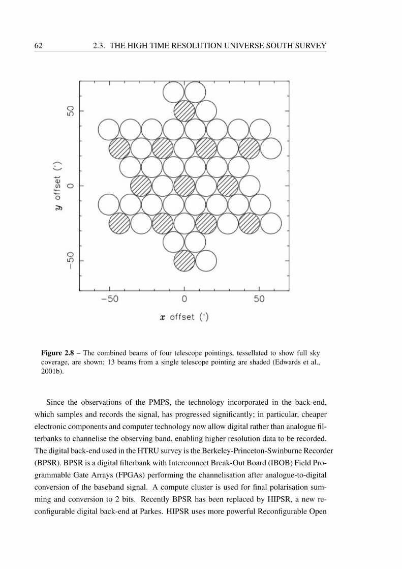
62 2.3. THE HIGH TIME RESOLUTION UNIVERSE SOUTH SURVEY

Figure 2.8 – The combined beams of four telescope pointings, tessellated to show full skycoverage, are shown; 13 beams from a single telescope pointing are shaded (Edwards et al.,2001b).

Since the observations of the PMPS, the technology incorporated in the back-end,which samples and records the signal, has progressed significantly; in particular, cheaperelectronic components and computer technology now allow digital rather than analogue fil-terbanks to channelise the observing band, enabling higher resolution data to be recorded.The digital back-end used in the HTRU survey is the Berkeley-Princeton-Swinburne Recorder(BPSR). BPSR is a digital filterbank with Interconnect Break-Out Board (IBOB) Field Pro-grammable Gate Arrays (FPGAs) performing the channelisation after analogue-to-digitalconversion of the baseband signal. A compute cluster is used for final polarisation sum-ming and conversion to 2 bits. Recently BPSR has been replaced by HIPSR, a new re-configurable digital back-end at Parkes. HIPSR uses more powerful Reconfigurable Open

D P G THORNTON 63

Architecture Computing Hardware (ROACH) FPGAs for the channelisation. The HIPSRcompute cluster uses Graphical Processing Units (GPUs) as well as CPUs for higher levelprocessing.

Each beam of the MB receiver consists of two signals from two orthogonal polari-sations. These 26 feeds are downconverted from ν = 1.18 → 1.58 GHz to ν = 0 →0.4 GHz. The baseband signals are then digitally Nyquist sampled (i.e. νsamp = 800 MHz)at 8 bits before passing to the FPGAs of BPSR. The FPGAs then split the signal into1024 × 0.390625 MHz channels. The baseband samples from each polarisation and eachchannel are accumulated for 25 samples and detected, giving a sample integration time oftsamp = 64 µsec, represented by a 32-bit number. These samples are further grouped into10-second blocks and scaled according to the mean and standard deviation in the block.Finally, the two polarisation pairs for each 64 µsec sample for each channel and each beamare summed and scaled to a 2-bit number to reduce the quantity of data to be stored; thistakes place on the compute cluster, these samples are then written to disk as filterbank data.The data are written to tape at Parkes, all data is also transferred electronically to SwinburneUniversity of Technology, Melbourne, where it is again written to tape. Upon completionof writing two full copies to tape the data are deleted from the compute cluster.

BPSR has a shorter sampling time and narrower channels than the PMPS analogueback-end (250 µs and 3 MHz for the PMPS respectively). This improves the sensitivity ofthe HTRU south survey to narrow-pulse, short-period, high-DM pulsars. In addition, 2-bitsampling improves dynamic range and resilience to RFI.

64 2.3. THE HIGH TIME RESOLUTION UNIVERSE SOUTH SURVEY

2.3.2 Survey regions

The HTRU south survey is split into three different parts, the low-, mid- and high-Galacticlatitude regions (see Table 2.1 and Figure 2.9). The HTRU survey began in 2008, with100% of the mid- and low-latitude, and 76% of the high-latitude survey observed to-date.

Figure 2.9 – An Aitoff projection of the Galactic regions covered by the HTRU southern survey.Red is low-, blue is mid- and green is high-latitude. The high-latitude survey is approximatelythe visible sky using the Parkes 64-m radio telescope.

The three survey regions were designed with different goals. The low-latitude surveyhas pointings twice the length of the PMPS, and with the improved temporal and spectralresolution aims to detect faint, high-DM, fast pulsars undetectable in the PMPS. The mid-latitude survey extends the PMPS region; while the pointings are shorter than for the PMPSthe limiting flux density is still lower for a large region of parameter space, particularlyMSPs (see Figure 2.10). The short (270 s) pointings of the high-latitude survey aim toprovide a “snapshot” of the high time resolution radio sky at 1.1 < ν < 1.5 GHz whichis visible with the 64-m Parkes. One of the aims of the high-latitude survey is to look forhighly dispersed narrow pulses originating from outside the Galaxy.

D P G THORNTON 65

Survey High Mid Low

Region δeq < +10 240 < l < 30 280 < l < 30

|b| < 15 |b| < 3.5

τobs 270 540 4300Nbeams, total 443287 95056 15990tsamp(µs) 64 64 64Btotal(MHz) 400 400 400Bchan(MHz) 0.390625 0.390625 0.390625nchan 1024 1024 1024Data Length (samples) 1022 1023 1026

Data per Beam (GB) ∼ 1 ∼ 2 ∼ 16

Total Data (TB) 435 190 250

Table 2.1 – Search parameters for the three sections of the HTRU south survey (Keith et al.,2010).

2.3.3 Sensitivity

The radiometer equation (Equation 2.1) quantifies how an increased total bandwidth andintegration time lowers the limiting flux density of a survey. Observing bandwidth is limitedby the receiver, or by the data rates which can be processed and stored. A compromise mustbe made between sensitivity and time required for the survey to determine the integrationtime, τobs. Different regions of the sky also have different effects on the observations. In thedirection of the Galactic plane there is an increase in the electron column density that affectsboth the DM and scattering. Also, there is a greater abundance of synchrotron emission inthe direction of the Galactic plane which affects the sky temperature. In the low-latituderegion Tsky has a mean of 7.5 K, compared to 2.5 K and 1.0 K for the mid- and high-latitudeareas respectively (at ν = 1.4 GHz). The minimum detectable flux densities for the threeHTRU survey regions, and for the PMPS, are shown in Figure 2.10.

66 2.3. THE HIGH TIME RESOLUTION UNIVERSE SOUTH SURVEY

Figure 2.10 – Minimum detectable flux density as a function of pulse period for a pulsar atDM = 100, 500, 1000 cm−3 pc in the three HTRU survey regions (low-, mid-, high-latituderegions are shown with the green, red, and blue lines respectively). The limiting flux densitieswere calculated using a minimum detectable SNR of 9, and the mean sky temperature of eachregion. For comparison the sensitivity of the PMPS is also shown (dashed black lines).

2.3.4 RFI removal

There is considerable RFI in the vicinity of Parkes. This includes satellite RFI (νRFI =

1.525− 1.559 GHz). There is a hardware filter is in place to remove this part of the observ-ing band. Once all channels with RFI are nulled in the data, the typical total useful band-width is approximately 0.340 GHz. There is also dynamic RFI that is sometimes present. Itis of course necessary to mitigate for this in each observation as much as possible to max-imise sensitivity to pulsars and single pulses. While pulsars and single pulses are narrow,the presence of RFI at the very least raises the noise floor of the observation, requiring ahigher flux density of the source for a given SNR.

The most extreme form of RFI rejection is intervention by the observer. Because ofthe digital flexibility of BPSR the observer is able to see the band-pass (the relative powerin each channel across the observing band), the zero-DM time-series and a DFT of thetime-series in close-to real time. The observer can then identify periods of wide-band RFI,

D P G THORNTON 67

which it would be difficult or impossible to excise, and they can choose to abandon theobservation. As the RFI is often direction dependent the observer may either be able toobserve a section of the survey with the telescope at a different azimuth and elevation, ortry to confirm previous candidates from the survey.

The HTRU survey maintains a list of channels within the observing band that alwayscontain RFI. These narrow regions of the band are not included in any searching of the data.This includes the channels which are blocked by a hardware filter to cut out satellite RFIat the top of the band. More subtle forms of RFI excision are performed on the filterbankdata prior to any searching. The first is that each channel of the filterbank data is searchedfor periodicities with a DFT. Any channels found with any signal with SNR > 15 are notincluded in further processing. The SNR in just a single channel of a pulsar would beconsiderably lower.

In addition to channel rejection, the zero-DM time-series is searched for bright peaks(SNR > 5). If found, the corresponding samples in all channels are replaced with randomvalues indistinguishable from the noise in the observation. In this way non-dispersed burstsof radiation should be removed. In addition to zero-DM bursts, this effectively removesbright low-DM pulses, where DM < 0.12

(w

64µs

)cm−3pc.

2.3.5 HTRU Fourier and single pulse searching

HTRU search data arrives at Jodrell Bank on LTO-4 tapes, each of which stores approx-imately 800 GB of data. The data are transferred from these tapes onto temporary harddisk storage ready for processing. The searching, candidate generation, and sifting are allperformed on the Hydra computing cluster at Jodrell Bank (see Figure 2.11). Hydra iscomprised of a head node and tens of processing nodes. A processing node carries out thepulsar and single pulse searching and writes the results to a network location (see Figure2.12).

All telescope pointings, corresponding to a set of 13 simultaneously observed beams,are independent of every other pointing. For the high-latitude survey the storage capacityof a processing node is large enough to store 13 completely searched beams (includingraw data, intermediate data, and final candidates). In processing the high-latitude survey,observation times (UTCs) are used to group beams from the same pointing (which have thesame UTC). A processing node then Fourier domain and single pulse searches all 13 beamsin turn.

68 2.3. THE HIGH TIME RESOLUTION UNIVERSE SOUTH SURVEY

Figu

re2.

11–

Asc

hem

atic

show

ing

com

putin

gcl

uste

rlev

else

arch

ing

ofth

eH

TR

Uhi

gh-l

atitu

desu

rvey

.

D P G THORNTON 69

Figu

re2.

12–

Apr

oces

sing

node

leve

lsch

emat

icsh

owin

gth

edi

ffer

ents

tage

sof

Four

ier

dom

ain

and

sing

lepu

lse

sear

chin

gfo

rth

eH

TR

Uhi

gh-

latit

ude

surv

ey.

RFI

:R

FIre

ject

ion;

DD

:de

disp

ersi

on;

DFT

:Fo

urie

rtr

ansf

orm

stag

e;Se

ek:

dete

ctin

gan

dgr

oupi

ngpe

riod

iciti

esin

the

pow

ersp

ectr

a.

70 2.3. THE HIGH TIME RESOLUTION UNIVERSE SOUTH SURVEY

HTRU search details

The data are dedispersed to 1436 DMtest values between 0 and 2000 cm−3 pc; the maximumvalue is chosen to be sensitive to the highest DM pulsars in the Galaxy. In addition tohigh-DM pulsars this upper limit for DMtest has enabled the discovery of highly dispersedextragalactic single pulses (see Chapters 5 and 6).

The time-series are Fourier transformed, harmonically folded, and threshold searchedusing the program seek which uses the FFTW library to perform the real-to-complex DFT(Frigo & Johnson, 2005). The output from seek is a list of pulse periods, the number ofharmonic folds, the DM, and the SNR of each candidate dispersed periodic signal. As dis-cussed in Section 2.1.3, these may be related harmonically or at similar DMs, in which casethey may be the same signal independently discovered in multiple time-series. ph-bestaims to combine these multiples, limiting the total number of candidates to 100 per beam.

Each candidate is a repeating signal which the software has identified: there has beenno analysis of the signal and its properties except its presence in the Fourier spectrum. Eachcandidate is therefore further refined by using dspsr (Hotan, van Straten & Manchester,2004) to fold the raw data at the period indicated by the Fourier spectrum, preserving 16subbands and 32 subints. A fine search in P and DM is then performed on this foldeddata to optimise the SNR of the pulse profile. This SNR can then complement, and becompared to, the SNR from the DFT power spectrum. The folded data are included in thefinal candidate file (along with the optimised parameters) for human inspection. The finalso-called phcx candidate files are an xml format containing the necessary data to producea candidate plot like Figure 2.13. xml is chosen as the flexibility and accessibility of thedata format provide the opportunity for further filtration and sorting of candidates.

D P G THORNTON 71

Figure 2.13 – A candidate from the HTRU survey showing the initial and optimised param-eters. The folded data are shown, including the fully averaged pulse profile (lower left) andthe pulse profile in each subint and subband (top- and middle-left grayscale). Also shown isthe amplitude spectrum SNR as a function of DMtest, and a bullseye plot (grayscale top-right)pulse profile SNR as a function of P and DM is shown from pdmp. Note that this candidateappears to be detected across the observing band, and is “on” for the duration of the observa-tion. This candidate was confirmed as a real MSP - PSR J2322−2650. See Chapter 4 for moreinformation.

The number of pulsar candidates from the HTRU survey is enormous; 100 candidatesfrom each beam gives ∼ 5 × 107 candidates for the high-latitude survey alone. For asingle user to look at all these would take over one year assuming one second to look ateach candidate 24 hours a day; not a feasible undertaking. An artificial neural network istherefore used to attempt to isolate the best candidates for human inspection.

2.3.6 Artificial neural network

An artificial neural network (ANN) is a machine learning pattern recognition techniquewhich aims to categorise datasets. The ANN condenses an input vector of numbers de-

72 2.3. THE HIGH TIME RESOLUTION UNIVERSE SOUTH SURVEY

scribing a candidate, via a series of weighted summations, into an output vector whosevalues indicate membership of a set.

In the pulsar ANN the input layer is a vector of heuristics which describe a candidate(see Table 2.2). In general, an ANN has a number of hidden layers, each with any numberof elements (defined at the time the net is constructed), which are connected to all theelements of the preceding layer (the input layer or another hidden layer). Finally an outputlayer, formed of just two elements, provides a simple indication of candidate category. Apulsar ANN attempts to separate candidates into two categories - pulsar and not pulsar -hence the two elements in the output layer (see Figure 2.14). In general, increasing thenumber of hidden layers allows an ANN to reproduce more complex behaviour; for theHTRU survey a single hidden layer is found to be sufficient.

Figure 2.14 – A schematic showing a generalised configuration of an ANN, each dotted lineimplies a “neural connection” and weight, the “neurons” (represented as circles) calculate theweighted sum of their inputs and produce an output value from an activation function. Theinformation flow in this schematic is from bottom to top. Figure from Bates et al. (2012).

Each connection between neurons corresponds to a weight, and each neuron calculatesthe weighted sum of connections going into it. Each neuron then calculates an output valueto pass-on using an activation function. The logistic sigmoid function is commonly used asactivation function because it can reproduce linear or non-linear behaviour depending on

D P G THORNTON 73

its input.

ANNs must be trained - that is, the weights between neurons must be set for maximalsuccess in classification of a training set. The training set is a set of candidates where boththe input and output layers are defined. A user has to pre-classify the training set and setthe output layer accordingly (pulsar = 1 not pulsar = 0 for a true pulsar and vice-versa foran RFI/noise candidate). Initially, the weights are set randomly and the outputs calculated.A method of back propagation is then used iteratively to modify these weights such that theoutput layer tends towards correctly classifying as much as possible of the training set. Asecond set of candidates, also pre-classified, is used for verification purposes.

The HTRU survey uses the Stuttgart Neural Network Simulator (SNNS1). There are 22numbers used to describe a candidate (outlined in Table 2.2); these 22 numbers form theinput layer. The single hidden layer also has 22 neurons. The output layer has two neurons(pulsar and not pulsar) whose values indicate whether the input heuristics were from apulsar candidate.

1http://www.ra.cs.uni-tuebingen.de/SNNS/

74 2.3. THE HIGH TIME RESOLUTION UNIVERSE SOUTH SURVEY

Score Number Description

1 Best Period, P2 Best DM3 Best SNR4 Pulse Width, Wobs

5 χ2 value of pulse profile and sin curve6 χ2 value of pulse profile and sin2 curve

7 χ2 value of pulse profile and Gaussian fit8 Full-width half-maximum of Gaussian fit9 χ2 value of pulse profile and two Gaussians fit10 Mean full-width half-maximum of two Gaussians fit

11 Offset of profile histogram from zero12 max.(profile histogram)/max.(fitted Gaussian)13 Offset of score 11 and profile gradient histogram

14 SNRdata/√

(P −Wobs)/W

15 SNRfit/√

(P −Wobs)/W

16 abs.(DMfit − DMbest

17 χ2 value of DM-SNR curve fit

18 RMS of the position of peaks in all sub-bands19 Average of correlation coefficients for all pairs of sub-bands20 Sum of correlation coefficients for all pairs of sub-bands

21 Number of peaks in pulse profile22 Area under pulse profile after mean subtraction

Table 2.2 – ANN heuristics for the HTRU survey processing at Jodrell Bank Centre for Astro-physics (Bates et al., 2012).

Once the net has been trained, it is applied to all pulsar candidates from the HTRUsurvey. The output scores are stored and those candidates with pulsar >0.5 and not pulsar

<0.5 are inspected by a human. This filtering routinely reduces the number for human

D P G THORNTON 75

inspection by a factor ∼ 100. The ANN used at JBO is able to identify 85% of pulsars(P > 10 ms) and 65% of MSPs (P < 10 ms) (Bates et al., 2012). The ANN provides auseful first look at the data but it is also important to look at other high-SNR candidateswith plausible P and DM values, particularly those with P < 10 ms. Regardless of ANNscores, all candidates are stored on disk and themselves form a derivative dataset to minefor pulsars with new techniques.

2.3.7 Human inspection

The final stage of candidate selection is human inspection. Currently in the HTRU surveythis is done for those that are scored highly by the ANN and for high-SNR MSP candidates.There are three basic categories of classification from human inspection - noise, RFI, orcandidate pulsar. The amount of data is such that noise fluctuations will sometimes resultin candidates which exceed the SNR threshold (see Figure 2.15).

Figure 2.15 – A noise candidate from the HTRU survey. While the spectral SNR is 23 theoptimised SNR (from folding) has fallen to 5.6. There is also no discernible broadband orpersistent emission, and the peak of the folded profile consists of just a single sample, againindicative of noise.

76 2.3. THE HIGH TIME RESOLUTION UNIVERSE SOUTH SURVEY

RFI candidates are usually easy to distinguish in the candidate plots. Often the signalis narrowband: the signal bandwidth is smaller than the total observing bandwidth. This isa typical feature of some types of RFI and thus candidates of this type are easily rejected.Similarly, the folded profile subbands shown in the candidate plot means that the user cantell if the pulsar was detected throughout the observation; temporally narrow signals arealso typical of RFI. The user must however be mindful of intermittent pulsars which mayswitch “on” or “off” during an observation however (Kramer et al., 2006a).

Figure 2.16 – A candidate from the HTRU survey which is an example of RFI. This candidateshows detected pulsations across only a small fraction of the observing band, and only during asmall fraction of the total integration time, strongly indicative of RFI. In addition, P = 0.47 mswould be dispersed within a channel to greater than the pulse period at a DM of 296 cm−3 pc -this can not have been a truly dispersed signal. The higher “harmonics” of DM = 296 cm−3 pcin the DM-SNR plot are due to the pulse wrapping over an integer number of pulse periods.

2.3.8 Candidate follow-up

When a strong pulsar candidate is identified (e.g. Figure 2.13) it is followed-up with aconfirmation observation. For MSPs this consists of a search observation at the positionof the centre of the beam in which the candidate was detected. The data is folded at the

D P G THORNTON 77

optimised period of the candidate, and is corrected for the candidate DM. pdmp is used tooptimise these nominal values and the observer checks for the detection of the pulsar. MSPsare often found in binaries and the apparent pulse period could be significantly differentfrom the original search period due to orbital Doppler shifting. If the pulsar is not apparentthen the data are dedispersed and searched for periodicity in the power spectrum. Fornormal pulsars the data is folded during the observation at the nominal pulse period; pdmp’sincremental changes are then able to directly optimise P and DM.

If confirmed, the new pulsar will be gridded. Gridding is a series of 5 observations,one at the position of the centre of the confirmation beam, and four equally spaced singlebeam pointings, separated by a half-power beam-width, from this nominal position. TheSNR of any detections in these five beams is then used to constrain the position. The newlyconfirmed pulsar is then assigned the best position from gridding, which is then refined vialong-term timing.

Confirmation and gridding observations are taken with the Parkes 64-m radio telescope,unless the candidate is at Decl. & −30 where the 76-m Lovell telescope at Jodrell Bankmay be used. The ongoing timing of HTRU pulsar discoveries then continues from thesame observatory.

2.3.9 Single pulse searching in the HTRU survey

The HTRU survey search pipeline uses the dedispersion routine dedisperse all. Forcomputing efficiency the single pulse search is performed by dedisperse all on thetime-series while they are still in the Random Access Memory (RAM) of the computer.

In addition to searching the full temporal resolution time-series (tsamp = 64 µ secs),each is searched after boxcar matched filtering. In the HTRU survey 2n adjacent samplesare summed, where n = 0 − 9, greatly improving sensitivity to bursts with widths up to32 ms.

A SNR threshold for single pulses is necessary to keep the number of candidates at amanageable level. Following the calculations of Burke-Spolaor et al. (2011b) the numberof independent trials, Nt, (possible locations for a single pulse) in an observation is

Nt = NDM

NBC∑i=0

Nsamp

2i(2.11)

78 2.3. THE HIGH TIME RESOLUTION UNIVERSE SOUTH SURVEY

where NDM is the number of DM trials, NBC is the number of matched-filter widths used,and Nsamp is the number of samples in a each dedispersed time-series. The error functioncan then be used to find the number of Gaussian distributed statistical noise samples, Nnoise,which would exceed a certain SNR threshold, SNRthreshold. For a single beam of the high-latitude HTRU survey NDM = 1436, NBC = 9, and Nsamp = 4.2× 106 (see Figure 2.17).

Figure 2.17 – The number of Gaussian noise samples which will exceed a given SNR thresholdin a HTRU high-latitude beam. The chosen SNR limit is shown with the black dashed line.

The SNRthreshold is chosen to minimise the number noise candidates while not rejectingreal candidates. For SNRthreshold = 6 then Nnoise ≈ 12. To reduce this number, othercharacteristics not expected of noise can be exploited. Of course, real broadband singlepulses have non-Gaussian statistics and may appear in multiple DM and boxcar-width trials- this property is also used to reject statistical fluctuations. In the case of the HTRU survey,SNRthreshold = 6 was therefore chosen as a suitable threshold after inspection of candidates.

Dispersion is not expected in terrestrial signals, which commonly have a peak in SNRwhen DMtest ≈ 0 cm−3 pc. By restricting candidates to those with a peak SNR at DMtest >

DMcut the number of non-dispersed RFI candidates, which would otherwise pass for hu-man inspection, is greatly reduced. In the HTRU survey this threshold is set to DMcut =

3 cm−3 pc.

D P G THORNTON 79

Sensitivity

It is useful to consider how sensitive the HTRU survey is to single pulses, particularly asa function of DM. The ability to evaluate this will become important when consideringpopulations of bursts and their DMs. A modified version of the radiometer equation forsingle pulses is used to calculate the peak intrinsic flux density a source would need tohave in order to be detected in the HTRU single pulse search pipeline. In the case of singlepulses, it is the observed width of the pulse, Wobs, which is important to its detectability.Wobs is defined as

Wobs =(W 2

int +W 2scatt +W 2

DM +W 2samp +Wchannel

)1/2, (2.12)

where Wint is the intrinsic width of the burst, WDM is the width induced due to DMtest

not being an exact match to the sources true DM, Wscatt is an increased observed widthof a pulse imparted during propagation, Wchannel is the dispersive smearing within a singlechannel, and Wsamp is smearing of a pulse due to the finite sampling time of the signal.τchannel is calculated from system parameters to be

τchannel = 8.3× 103 secs

(DM

cm−3pc

)(νmid

MHz

)−3(Bchan

MHz

), (2.13)

where νmid is the central frequency of the observing band, and Bchan is the channel band-width. Scattering is more complicated; within the Galaxy there is an empirical relationfound by Bhat et al. (2004) which relates the scattering timescale, Wscatt, to the DM. Therelation was derived from multi-frequency measurements of pulsars throughout the MilkyWay and as such it may not be applicable to propagation through the ionised intergalacticmedium. There is also a spread of at least two orders of magnitude inWscatt for a given DM:in calculating the required peak flux density of a burst to be detected in the HTRU data, aspread of one order of magnitude on Wscatt either side of the Bhat et al. (2004) relation isused (see Figure 2.18). The limiting peak flux density Speak, for a burst is defined as

Speak =σβ(Tsys + Tsky)

G√npBWobs

, (2.14)

where σ = 9 is the minimum acceptable signal to noise ratio, β = 1.07 is a factor from

80 2.3. THE HIGH TIME RESOLUTION UNIVERSE SOUTH SURVEY

digitisation (Kouwenhoven & Voute, 2001), Tsys and Tsky are the system and sky tempera-tures respectively, G = 0.735 Jy K−1 is the telescope gain, and B = 340 MHz is the totaluseful observing bandwidth.

Figure 2.18 – The minimum peak flux density of a single burst as a function of DM. Speakis peak flux density a single pulse must have in order to be detected with an SNR of 9 in theHTRU survey. The intrinsic widths are shown; dashed-dotted lines correspond to Wint = 64 µs(the raw sampling rate), dashed lines to Wint = 2 ms, and solid lines to Wint = 30 ms. Theblue lines correspond to a degree of scattering a factor of ten lower than the Bhat et al. (2004)scattering model, and the red lines a factor of 10 higher.

For DM & 500 cm−3 pc the apparent pulse width is dominated by scattering. As aburst appears wider it becomes harder to detect; this calculation suggests that scattering isdetrimental to the detectability of high-DM bursts. In order for a Wint = 2 ms single pulseto have the same SNR when DM = 1000 cm−3 pc as when DM = 500 cm−3 pc its peakflux density would have to be approximately a factor of 10 higher, even in the low scatteringregime shown in Figure 2.18.

The data from each of the 13 beams of the multibeam receiver are available on the sameprocessing node so it is possible to take advantage of the fact that many single pulse sourcesof RFI often appear simultaneously in multiple beams (Burke-Spolaor et al., 2011a). Thishappens because the source is not in any of the beams at all but almost certainly in thedirection of the horizon (the 64-m Parkes radio dish cannot point to the horizon). The RFI

D P G THORNTON 81

are therefore likely in a sidelobe of the beam patterns of the receiver or in the near-field.The sources of RFI are instead extremely bright and arrive at the feed horns over the edgeof the dish. When all 13 beams of a pointing have been processed we can combine thesingle pulse candidates, and reject any which are temporally associated and appear in > 9

beams.

A number of heuristics and sections of reduced data are included in a single pulsecandidate file. High SNR single-pulse candidate files include the dedispersed time-seriesaround the pulse position in all 13 beams, the time-series in which the single pulse has thehighest SNR, the time-series with DMtest value one step above and below, and the zero-DMtime-series. The single pulse SNR as a function of boxcar matched filter width and of DMis included, as is small section of non-dedispersed filterbank data centred on the pulse (seeFigure 2.19). All these diagnostics allow human inspection to quickly identify potentiallyinteresting candidates.

82 2.3. THE HIGH TIME RESOLUTION UNIVERSE SOUTH SURVEY

Figure 2.19 – A single pulse candidate from PSR J1843−0211. The dedispersed time-series(dedispersed with the DM which gives the highest pulse) for all 13 beams of the receiver areshown (top left), the dedispersed time-series and one DM step above and below, the zero-DMtimeseries shown (bottom left). The non-dedispersed section of filterbank data (bottom right) isoverlaid with the dispersive sweep expected of pulse with DMtest (white line). In the top rightthe SNR as a function of DMtest and of boxcar matched filter width are shown. Basic parametersof the pulse (SNR, DM, best matched filter width, Right Ascension and Declination) are alsoshown. In this case the dispersed sweep of the pulse is visible across the band as well as in thededispersed time-series (only in beam #6). Note that the pulse is not seen in any of the otherbeams of the receiver, or in the zero-DM time-series.

A large proportion of single pulse RFI is caused by bright, narrowband, short timescalebursts of radiation. These are sufficiently bright in a single part of the band that the receiversaturates. This causes the gain to fall across the full observing band. The result is a narrow-band pulse where the levels across the rest of the band are depressed. At DM = 0 cm−3 pcthe average of the channels at this sample may be zero or negative and does not look likeRFI, where a peak in the zero-DM time-series would be expected. However, when dedis-persed however the average is often positive, resulting in an apparent dispersed detection

D P G THORNTON 83

(e.g. Figure 2.20). Human inspection allows the quick rejection of the majority of RFI,including this type which can pass the RFI rejection.

Figure 2.20 – A single pulse RFI candidate showing a narrowband pulse which has saturatedthe receiver. The zero-DM timeseries shows no significant detection but the dedispersed time-series do.

An xml candidate format for the single pulse candidates, similar to the phcx pulsarcandidates, has been developed, enabling future searching and narrowing of the candidaterepository. An implementation of an ANN, when a sufficient training set has been devel-oped, may also prove useful.

Chapter 3

Discovery of five recycled pulsars in theHigh Time Resolution Universe survey

This chapter is based on a paper in preparation entitled “The High Time Resolution Uni-verse survey: Discovery of 5 Millisecond Pulsars & the optical detectability of white dwarfcompanions”

D. Thornton, M. Bailes, C. Bassa, S. Bates, N. D. R. Bhat, M. Burgay, S. Burke-Spolaor,D. J. Champion, N. D’Amico, A. Jameson, S. Johnston, M. J. Keith, M. Kramer, L. Levin,A. Lyne, S. Milia, C. Ng, A. Possenti, B. Stappers, W. van Straten

In this chapter five partially and fully recycled pulsars discovered in the HTRU surveyare presented and analysed. Their spin periods range from 2.01 ms to 66.29 ms, and threeare in binary systems with companions that are most likely to be white dwarfs, one isin an orbit with either a heavy white dwarf or another neutron star, and one, which weconclude is a member of the growing class of disrupted binary pulsars, is isolated. Giventhe exciting possibility of testing evolutionary and gravitational theory through the studyof pulsar-white dwarf binaries, I analyse the probability of an optical detection of the whitedwarf companions to pulsars in the HTRU survey sample.

84

D P G THORNTON 85

3.1 Introduction

The progenitors of neutron stars are massive stars (M = 8 − 10 M); a large fractionof which are found in binary systems (Lada, 2006). The more massive of the two starswill have a shorter lifetime and, if sufficiently massive, undergo a core collapse supernova(ccSN) first (see Section 1). The remnant of the stellar core may form a neutron star (NS),which in turn could be a detectable pulsar. The fact that most of the normal pulsars ob-served are isolated implies that the majority of massive stellar binaries disrupt during thefirst ccSN. Pulsars that remain gravitationally bound to their companion post-ccSN maythen have their evolution affected by the companion, possibly recycling them (Alpar et al.,1982). The recycling - or spin-up stage - shortens the spin-period and reduces the surfacemagnetic field strength, in turn allowing them to be detectable as radio pulsars for billionsof years. See Chapter 1 for a more detailed discussion of the pulsar recycling process.

3.2 Discovery and Timing

The five pulsars presented here were discovered in the HTRU survey for pulsars and tran-sients (Keith et al., 2010). Survey observations are made with the 64-metre Parkes radiotelescope using the 13-beam 21 cm multibeam receiver. Each beam’s half-power beam-width is approximately 14 arcminutes. The 13 simultaneous beams enable rapid coverageof the sky compared to a single beam system. The survey has an observing band centredat 1352 MHz and has a useful bandwidth of 340 MHz. The HTRU survey is split into 3areas: the low-, mid- and high-Galactic latitude regions. The discoveries presented hereare from the mid-latitude region which is centred on the Galactic plane and has pointingsof 540 seconds in duration. The region covers −120 < l < +30 and −15 < b < +15

in Galactic coordinates. See Chapter 2 for a more detailed discussion of the HTRU survey.

The data were processed using the Fourier transform based pulsar search pipeline de-scribed in Chapter 2 and Keith et al. (2010). The discoveries described here were initiallyidentified using an artificial neural network (ANN) which aims to highlight the best candi-dates from the survey for human inspection (Bates et al., 2012; Eatough et al., 2010). Afterinspection, confirmation observations are taken at the sky positions of the survey beamsdeemed to contain the best candidates. These confirmations are performed with the 64-mParkes dish or the 76-m Lovell Telescope at Jodrell Bank. Four of the five pulsars presentedhere, PSRs J1227−6208, J1405−4656, J1431−4715, and J1653−2054, are in orbit with a

86 3.2. DISCOVERY AND TIMING

Table 3.1 – Observing system details for the timing observations made as part of this work.Note the specifications for the Lovell Telescope take into account the removal, as standard, ofa section of the observing bandwidth due to contamination by RFI.

Telescope Centre Freq. BW nchan 〈τobs〉(GHz) (GHz) (s)

Parkes 64-m 0.732 0.064 512 9001.369 0.256 1024 6003.094 1.024 1024 900

Lovell 76-m 1.524 0.384 768 1800

binary companion, while one, PSR J1729−2117, is isolated.

As well as being independently discovered in the mid-latitude region of the HTRU sur-vey PSR J1227−6208 was also identified by two separate groups in the Parkes MultibeamPulsar Survey (PMPS) (Mickaliger et al., 2012; Knispel et al., 2013). The PMPS discov-eries happened around 10 years after the survey was completed and are illustrative of largepulsar surveys providing the opportunity to discover new pulsars with increasing comput-ing power and new techniques many years after the data was recorded. All observations,timing, and analysis of PSR J1227−6208 presented here are independent work.

Once confirmed, the new pulsars were timed regularly with digital filterbank (DFB)backend systems; PSRs J1653−2054 and J1729−2117 with the 76-m Lovell telescope atJodrell Bank Observatory (JBO) and PSRs J1431−4715, J1405−4656, and J1227−6208with the 64-m radio telescope at Parkes (see Table 3.1). The pulsars timed with the Lovelltelescope were observed approximately once per week, whereas those observed using theParkes radio telescope were observed more sporadically, while maintaining phase coher-ence, with one case of an approximately 80 day gap between observations.

Each observation resulted in a pulse time-of-arrival (TOA) measurement. The temporalvariation of these TOAs is then modelled by a series of astrometric, spin, and, if necessary,orbital parameters. This model is modified and fit by comparison with further TOA obser-vations (described in Lorimer & Kramer 2005). Parameters were fitted using the TEMPO2software package (Hobbs, Edwards & Manchester, 2006) using the DE 414 solar systemephemeris from JPL for barycentric correction1. The best fit parameters for the five pulsarsare provided in Table 3.2.

1http://ssd.jpl.nasa.gov/?ephemerides

D P G THORNTON 87

Figure 3.1 – A plot of pulse period derivative P against pulse period P . Pulsars in binariesare represented as open circles, isolated pulsars as red round points, DNS systems as greencircles (see Table 3.3), the four newly discovered pulsar binaries are plotted as stars, and theisolated pulsar, PSR J1729−2117, as a large diamond (see Table 3.2). Only Galactic pulsarswith P < 100 ms and P < 10−16 and DNS systems are shown.

3.3 Results

The pulse periods for the systems range from 2.01 ms (PSR J1431−4715), placing it amongthe 20 fastest spinning pulsars, and 66.29 ms (PSR J1729−2117), one of the longer periodsfor a recycled pulsar (Manchester et al., 2005). While the five pulsars do not represent anyfundamentally new type, together they comprise systems from across the range of knownrecycled pulsar and binary types (see Figure 3.1). PSR J1729−2117, does not exhibit anydetectable periodic variation of the apparent pulse period that would be indicative of abinary companion, making it one of just two isolated recycled pulsars in the HTRU surveyto date; an interesting dearth when compared to previously known recycled pulsars, whichis discussed in Burgay et al. (2013).

To determine the masses of the companion in binary pulsar systems the orbital period,Porb, and the projected semi-major axis of the pulsar’s orbit, ap sin(i) are measured. These

88 3.3. RESULTS

two quantities are related via the mass function (Equation 3.1). The mass function for arange of inclinations can be used to derive a companion mass range; particularly a lowermass limit. In all calculations a canonical pulsar mass, Mp = 1.4 M is used; although itshould be that noted there is mounting evidence for pulsars more massive than 1.4 M (e.g.Demorest et al. 2010; van Kerkwijk, Breton & Kulkarni 2011; Antoniadis et al. 2013). Theability to measure the pulsar mass is one of the reasons for detailed measurements of binarysystems. It would be interesting, for instance, to determine if heavier pulsars have shorterspin periods, perhaps due to the mass accreted during spin-up (e.g. Jacoby et al. 2005). ForKeplerian orbits the mass function relates these quantities to Mc and Mp, the mass of thecompanion and pulsar respectively:

(Mc sin i)3

(Mp +Mc)2 =

4π2

G

(ap sin i)3

P 2orb

M. (3.1)

For a given inclination, i, a companion mass Mc can be determined. If the orbit is viewededge-on (i = 90) Mc is the minimum companion mass, i = 60 corresponds to the mediancompanion mass, and a maximum mass, Mc, is defined such that for randomly inclinedorbits the probability(Mc > Mc, max) < 0.05 (see Table 3.2).

D P G THORNTON 89

Figure 3.2 – Typical pulse profiles are shown for the five recycled pulsars discussed in thischapter. The top, middle, and bottom rows correspond to 3.1 GHz, 1.4 GHz, and 0.732 GHzrespectively. Blank plots correspond to non-detections. The observing times are given in Table3.1). All observations are taken with the 64-m Parkes radio telescope, except for the 1.4 GHzobservations and timing of PSRs J1653−2054 and J1729−2117, which use the 76-m Lovelltelescope at Jodrell Bank.

90 3.3. RESULTSPa

ram

eter

PSR

J122

7−62

08PS

RJ1

405−

4656

PSR

J143

1−47

15PS

RJ1

653−

2054

PSR

J172

9−21

17

Rig

htA

scen

sion

(J20

00)

12:2

7:00

.444

(3)

14:0

5:51

.424

1(5)

14:3

1:44

.614

5(5)

16:5

3:31

.014

(1)

17:2

9:10

.812

(2)

Dec

linat

ion

(J20

00)

−62

:08:

43.8

1(1)

−46

:56:

02.2

96(6

)−

47:1

5:27

.64(

1)−

20:5

4:55

.3(1

)−

21:1

7:.2

6.3(

5)G

alac

ticL

ongi

tude

()

+30

0.08

+31

5.90

+32

0.05

+35

9.96

+4.

49

Gal

actic

Lat

itude

()

+0.

59+

14.0

5+

12.2

5+

14.2

6+

7.22

Dis

cove

ryS/

N11.2

125.

012.0

11.5

13.7

Off

setf

rom

surv

ey0.

10.

050.

030.

040.

08

beam

()

TOA

Ran

ge(M

JD)

5590

1–56

331

5566

7–56

331

5575

6–56

022

5564

6–56

332

5552

9–56

334

P(m

s)34.5

2783

4648

(2)

7.60

2203

4325

0(9)

2.01

1953

440(

1)4.

1291

4528

4650

(2)

66.2

9290

0298

5(1)

P(×

10−

20)

15(1

)2.

81(3

)1.

38(4

)1.

14(1

)16

(1)

DM

(cm−

3pc

)36

2.6

13.8

959.4

56.5

234.9

S1.4

GH

z(m

Jy)

0.22

0.92

0.73

0.16

0.20

DM

Dis

tanc

e,d

(kpc

)8.

320.

580

1.53

31.

626

1.09

1

L1.4

GH

z(m

Jykp

c2)

15.2

0.3

1.7

0.4

0.02

τ c(G

.yr)

3.6

4.2

3.3

5.6

6.2

Bsu

rf(G

auss

)2.

3×

109

4.6×

108

2.2×

108

2.2×

109

3.3×

109

Blc

(Gau

ss)

9.4×

101

8.4×

102

1.0×

105

1.8×

103

2.7×

101

E(e

rgs−

1)

1.4×

1034

2.5×

1033

4.8×

1033

6.4×

1033

2.2×

1031

E/d

2(e

rgkp

c−2

s−1)

2.0×

1030

7.5×

1033

2.0×

1033

2.4×

1033

1.9×

1031

PS

hk(×

10−

20)

0.32

1.0

0.1

0.2

4.7

Por

b(d

)6.

7210

1336

(4)

8.95

6419

83(9

)0.

4497

3915

1(1)

1.22

6815

23(1

)–

asi

ni

(lts

)23.2

0062

(1)

6.56

7651

(8)

0.55

0113

(1)

0.68

8856

(5)

–T

asc

(MJD

)55

991.

1937

916(

8)55

692.

7393

69(2

)55

746.

1047

762(

2)55

584.

7284

29(3

)–

ε 15.

22(1

)×

10−

46(

2)×

10−

61.

52(3

)×

10−

4<

2×

10−

5–

ε 21.

028(

1)×

10−

33(

2)×

10−

6−

2.8(

4)×

10−

53(

1)×

10−

5–

e1.

1153

(1)×

10−

37(

2)×

10−

6<

1.7(

8)×

10−

5<

10−

5–

ω(

)26.9

5(7)

60(1

5)–

––

Mco

mp,m

in(M

)1.

290.

200.

127

0.08

0–

Mco

mp,m

ed(M

)1.

600.

250.

148

0.09

3–

Mco

mp,m

ax

(M

)12.4

50.

870.

471

0.28

1–

RM

Sof

fit(µ

s)10

6.8

30.0

36.4

27.9

195

Table 3.2 – See below

Table 3.2 - The measured and calculated parameters for the presented pulsar systems.Where required a canonical pulsar mass of 1.4 M has been used. The maximum compan-ion mass Mc, max is the 95% confidence level limit which is at an inclination of i = 18.The NE2001 model of Galactic electron density (Cordes & Lazio, 2002) has been usedto infer distance from the dispersion measure. PShk is the apparent spin period derivativecaused by the proper motion of the pulsar, this value is the maximum P expected for anominal MSP velocity of 85 km s−1 at the distance calculated from the dispersion measure(Toscano et al., 1999). None of the four binary systems have a highly eccentric orbit; be-cause of this the ELL1 binary timing model was used (suitable for low-e orbits) which uses

D P G THORNTON 91

the Laplace-Lagrange parameters ε1 and ε2 (Lange et al., 2001).

3.3.1 PSR J1227−6208

PSR J1227−6208 has measured values of P and P that place it in a region of the P − Pdiagram where mildly recycled pulsars are found (see Figure 3.1). This is consistent with ithaving been spun-up during unstable, short lived mass transfer in an HMXB spin-up phase(see Section 1.1.5).

It has an orbital eccentricity, e = 1.153(1) × 10−3, a period Porb = 6.72 days, and aprojected semi-major axis, ap sin(i) = 23.2 ls. Using Equation 3.1 and assuming Mp =

1.4 M, this leads to a minimum companion mass of Mc, min = 1.29 M if the system isviewed edge-on. The low eccentricity and high minimum companion mass are unusual:there are only 3 other systems known with e < 0.1 and Mc, min > 1.0 M.

PSR J1227−6208 is similar to other so-called Intermediate Mass Binary Pulsars (IMBPs);for example PSR J1435−6100 (Camilo et al., 2001) and PSR J2222−0137 (Boyles et al.,2013). PSR J1227−6208’s spin parameters are also similar to PSR J0609+2130 - an iso-lated pulsar thought to be the result of an HMXB which disrupted during the second ccSN(Lorimer et al., 2004). In an IMBP it is thought the companion was not sufficiently mas-sive to undergo a ccSN, resulting instead in the formation of a heavy CO or ONeMg WD.The minimum mass for the companion to PSR J1228−6208 is common for ONeMg WDs,which have a mass range around 1.1 − 1.3 M (Tauris, Langer & Kramer, 2012). This ishowever the minimum mass the companion may have: it is already close to the upper limitof ONeMg WDs, and to the Chandrasekhar mass limit. If the system was not edge-on thenthe companion mass would be higher and inconsistent with a heavy WD, indeed the mediancompanion mass Mc, med = 1.60 M (see Table 3.3.1).

For an inclination i < 71, Mc & 1.4 M, the companion may be a second NS andPSR J1227−6208 would be part of a DNS. Unseen as a pulsar in the survey observation,the second NS would have formed from a massive progenitor (8− 10 M), and the systemwould have evolved through an HMXB phase, hence the partially recycled pulsar. Com-paring to known DNS systems the eccentricity (e = 1.153(1)× 10−3) would be unusuallylow; see Table 3.3). The formation of DNS systems with such a small eccentricity appearsto be unlikely (Chaurasia & Bailes, 2005) and as such the eccentricity is the only charac-teristic of PSR J1227−6208 which suggests it is not a DNS system. The simulations ofDewi, Podsiadlowski & Pols (2005) and Chaurasia & Bailes (2005) do however appear to

92 3.3. RESULTS

Table 3.3 – Basic orbital and spin parameters for known DNS systems. Also included are thesame parameters for PSR J1227−6208.

Pulsar Spin period Orbital period Projected semi- Eccentricity, Companionmajor axis mass

P (ms) Porb (d) ap sin i (ls) e Mc, min (M)J0737−3039 22.69 0.102 1.415 0.088 1.250J1518+4904 40.93 8.634 20.044 0.249 > 0.83B1534+12 37.90 0.420 3.729 0.273 1.34J1756−2251 28.46 0.319 2.756 0.180 1.18J1811−1736 104.18 18.779 34.783 0.828 > 0.87J1829+2456 41.00 1.176 7.236 0.139 > 1.22B1913+16 59.03 0.322 2.341 0.617 1.38B2127+11C 30.52 0.335 2.518 0.681 1.354

J1227−6208 35.52 6.721 23.200 0.001 > 1.29

suggest that such low-eccentricity DNS systems could exist because of the possibility ofvery small ccSN kinematic kicks, although they would be extremely rare. Low-eccentricityDNS systems, however, would not lose energy via gravitational wave emission as quicklyas eccentric systems, and consequently will survive longer before merging.

With DM = 362.6 cm−3 pc PSR J1227−6208 appears to be located at a large distanceof 8.3 kpc. This would make an optical detection of a WD companion extremely difficult.Consequently, the best chance of measuring the masses in the system could come from themeasurement of post-Keplerian parameters.

Periastron advance

While the eccentricity of the orbit of PSR J1227−6208 is small, it is measurable, andis significantly higher than is typical for systems which have likely evolved through anLMXB phase (Phinney, 1992). It is possible to predict relativistic changes to the orbit dueto general relativity. These changes are quantified by the post-Keplerian parameters andare largest for eccentric orbits. One of the easiest to measure is a changing longitude ofperiastron,

ω = 3T2/3

(Porb

2π

)−5/31

1− e2(Mp +Mc)

2/3 rad s−1, (3.2)

where T = GM/c3, Porb is the orbital period, e is the orbital eccentricity, andMc andMp

are the companion and pulsar masses respectively. A measured ω constitutes a measure-

D P G THORNTON 93

ment of the combined masses, Mc +Mp and consequently constrains the companion mass.The prediction of Equation 3.2 is ω = 0.63 deg yr−1 for the PSR J1227−6208 system; todate no significant measurement of ω has been possible.

Shapiro delay

The radio pulses from a pulsar in a binary system are delayed as they cross the gravitationalpotential of the companion; this phenomenon is called Shapiro delay (Shapiro, 1964). Theelectromagnetic radiation takes a curved path around the companion, this bent path thencorresponds to a longer travel time, and delays in the pulse TOAs may be observed. Themagnitude of the delay depends on the relative position of the line-of-sight to the pulsarand the companion’s gravitational potential, which is orbital phase dependent. The pulsestake the longest path around the deepest part of the companion’s potential when the pulsaris at superior conjunction (orbital phase, Φ = 0.25). The magnitude of the observed delayalso depends on the viewing angle of the orbit. For a given companion mass the delay ismaximal for an orbital system viewed edge-on (i = 90).

The Shapiro delay, ∆S, is quantified by two post-Keplerian parameters, the range, r,and the shape, s. For low-eccentricity systems

∆S(Φ) = −2rln(1− s sin Φ), (3.3)

where Φ is the orbital phase (where Φ = 0 is the ascending node), r = TMc and s = sin i.The Shapiro delay is the same for every orbit of the system and so when the TOA residualsare folded modulo-Porb a characteristic shape in the timing residuals may be measured. Theorbital phase, Φ, dependence of this delay is given by Equation 3.3.

An observing program was undertaken using the 64-m Parkes radio telescope to obtainTOAs across the orbit. A global timing solution was made (as given in Table 3.2), fromwhich the astrometric and spin parameters were fixed. These TOAs were then fit for all theorbital parameters (Porb, Tasc, ap sin(i), ε1 and ε2) with fixed values of Mc and sin(i). Thereduced-χ2 (χ2

red) goodness-of-fit statistic was then calculated for each pair ofMc and sin(i)

values (see Figure 3.3). The results of these fits indicate that large sections of Mc − sin(i)

are still possible, however preferred values appear to be at high inclination angles. For acompanion mass of Mc = 1.29 M and i = 90 then χ2

red = 3.8; while for Mc = 1.4 Mand i = 71 then χ2

red = 1.3. This suggests that the binary may be a DNS system with

94 3.3. RESULTS

Figure 3.3 – The χ2red values calculated for a series of Mc and sin(i) values. All χ2

red > 5 wereset to be equal to 5 for sensible scaling. The constraints of a Keplerian orbit from pulsar timingwith a 1.4 M pulsar (blue) and for a 2.0 M pulsar (red) are also shown (see Equation 3.1).For a pulsar of these masses or between then the true values will lie on or between these lines.

i ≈ 71. There is however little change in χ2red along either the Mp = 1.4 M or the

Mp = 2.0 M Keplerian relationships defined by the mass function (Equation 3.1).

Figure 3.4 shows that the density of observations around superior conjunction (Φ =

0.25) is high enough that if the system were edge-on with a Mc = 1.29 M companionthen a measurable Shapiro delay would likely have been observed. Of course the lackof a Shapiro delay signal is consistent with a more massive companion. It is howeverimportant to note that some of the Shapiro delay may have been absorbed into the othertiming parameters.

PSR J1227−6208 has a single narrow pulse at an observing frequency of 1.4 GHz, at3.1 GHz a similarly narrow peak is detected. We have not yet made a detection at 0.732GHz. The pulse profile appears to be approximately 3.2 times wider at 1.4 GHz than at3.1 GHz. If this trend were due to scattering, and thus has a strong frequency dependence(∝ ν−4 then the the profile width at 0.732 GHz would be approximately 2 ms. This timewould not exceed the pulse period, consequently scattering would not be the reason thatPSR J1227−6208 is not detected at 0.732 GHz.

D P G THORNTON 95

Figure 3.4 – The residuals from the best fit global timing model for PSR J1227−6208 areshown plotted against orbital phase (these residuals have not had any Shapiro delay contributiontaken into account). In blue is the expected Shapiro delay for Mc = 1.29 M and i = 90; inred is the Shapiro delay for Mc = 1.4 M and i = 71, both are shown for Mp = 1.4 M.

96 3.3. RESULTS

3.3.2 PSR J1405−4656

The spin period, P = 7.6 ms, and period derivative, P = 2.81×10−20, of PSR J1405−4656are typical of fully recycled MSPs (see Figure 3.1), and are indicative of it having under-gone spin-up in a LMXB phase. The measured value of P can be affected in a numberof ways, one of these is the Shklovskii effect which is caused by a pulsar moving in theplane of the sky. This motion causes an apparent period derivative, PShk. In the case of PSRJ1405−4656 this contribution would be around 35% of the total measured, for a typicalMSP velocity of v = 85 km s−1 (Toscano et al., 1999). Consequently the P measured maynot be totally intrinsic, and there is likely a contribution from the Shklovskii effect. Thispresence of a Shklovskii effect of this magnitude does not, however, change any of theconclusions about this MSP’s evolutionary history.

The flux density of PSR J1405−4656 varies significantly between observations. Forinstance, the survey observation had a SNR of 125 in 600 seconds whereas during timingthere are many occasions when it was not detected in 1000 seconds. This is attributableto interstellar scintillation, which is caused by fluctuations in the density of the ionisedmaterial along the line of sight, which leads to ever-changing multipath propagation andresults in the radio waves constructively and destructively interfering. For a distant pulsar asingle fluctuation has relatively little effect, however for nearby pulsars a single fluctuationhas a proportionately larger effect. The scintillation bandwidth for this source at 1.4 GHzis around 400 MHz (Cordes & Lazio, 2002), this would mean that with the observing bandof the timing system (see Table 3.1) we would not expect to be able to discern individualscintles within the band - this is indeed the case. Because of the distance dependence ofscintillation it is usually most pronounced in relatively nearby pulsars (Stinebring et al.,2000). PSR J1405−4656, with DM = 13.89 cm−3 pc and d = 0.580 kpc, falls into thiscategory. There is no discernible broadening of the pulse profile which may be attributedto scattering between the 1.4 GHz and 0.732 GHz pulse profiles. This is to be expected forsuch a low DM pulsar (Bhat et al., 2004).

3.3.3 PSR J1431−4715

PSR J1431−4715 has the 14th shortest spin period of all known pulsars (P = 2.01 ms),and also a small spin-period derivative (P = −1.38 × 10−20 s s−1) . These values placePSR J1431−4715 firmly amongst the fully recycled MSPs in the bottom left of the P − Pdiagram (see Figure 3.1). The pulsar also exhibits significant, unmodelled, orbital-phase,

D P G THORNTON 97

Figure 3.5 – The top panel shows the timing residuals for PSR J1431−4715 which are foldedmodulo-Porb. The excess residuals which are not described by the timing model are centredaround superior conjunction, Φ = 0.25 (indicated by the dashed line). The lower panel showsthe same delays converted to an electron column density within the eclipsing region. In bothpanels there are observations at three frequencies; 1.4 GHz (green), 0.732 GHz (blue), 3.1 GHz(red).

Φ, dependent delays in the pulse TOAs. By plotting the TOAs modulo-Porb these excess de-lays are seen to occur around superior conjunction (Φ = 0.25), when the pulsar is directlybehind the companion (see Figure 3.5). They can be explained by an orbital phase depen-dent DM, with a period of excess DM lasting approximately 10% of the orbital period.This excess DM is attributed to the passage of the radio pulses through ionised materialsurrounding the companion (see Figure 3.6). The timing model described in Table 3.2was generated by excluding TOAs which are obviously associated with the eclipse region,0.1 < Φ < 0.4.

Multi-frequency observations (see Figure 3.2) indicate the eclipse duration depends onobserving frequency, with the 3.1 GHz observations showing a somewhat shorter eclipsethan at 1.4 GHz. The lower frequency observations (centred on 0.732 GHz) have not re-

98 3.3. RESULTS

sulted in a positive detection to date across the eclipse region (see Figure 3.5). We canconvert from the residual from the best fit timing model to the corresponding excess DMusing Equation 2.2. By approximating the depth of the eclipsing region as being equal toRecl the free-electron column density along the line of sight can be calculated (see Figure3.5). The magnitude of the column density is similar to other eclipsing systems; for exam-ple PSR J2051−0827 (Stappers et al., 1996) and PSR J1731−1847 (Bates et al., 2011).

Using multiple observations during different eclipses we find that there appear to besignificantly different TOAs at the same orbital phase within the eclipse region. The TOAswere measured during observations which were separated by several months, that is ∼ 102

orbital periods. As such, the amount or density of dispersive material must be variable onthis timescale. The width of the eclipsing region appears to be constant, suggesting it is thefree electron density which is variable as opposed to depth of the eclipsing region.

By using the measured semi-major axis of the pulsar orbit, ap, around the centre ofmass (in the edge-on, i = 90 case) the orbital separation for a circular system, A, is givenby

A = ap (1 + q) , (3.4)

where the mass ratio, q = Mp/Mc. Given that the eclipse duration is ≈ 10% of the orbitalperiod then the physical size of the eclipsing region Recl = ac/10 where ac is the semi-major axis of the companion orbit. Note that this is the size of the region which lies parallelto the line in the sky corresponding to the eclipse.

From the orbital separation and the mass ratio we determine the approximate distanceof the Roche lobe from the companion, RL, using

RL =0.49Aq2/3

0.6q2/3 + ln (1 + q1/3), (3.5)

from Eggleton (1983). In this case RL = 0.6 R, about half the size of Recl = 1.3 R (seeFigure 3.6). A significant amount of the material in the eclipsing region is therefore furtherthan RL from the centre of the companion. Material which is close to the Roche lobe caneasily be removed by a relativistic pulsar wind (Breton et al., 2013). This would mean someeclipsing material was not gravitationally bound to the companion and must therefore bebeing continually replenished (Stappers et al., 1996). This ablation of the companion may

D P G THORNTON 99

Figure 3.6 – A to-scale top-down diagram of the PSR J1431−4715 system for i = 90. Thered triangles indicate the extent of the eclipse region in the orbital plane, the black + symbolmarks the position of the inner Lagrange (L1) point, the companion and pulsar are marked asstars, the centre-of-mass of the system is marked by the blue + symbol with the orbits of thepulsar and companion shown as the large dotted circles. The black arrow indicates the line ofsight towards the Earth. The relative positions of the companion and pulsar are as they wouldbe at superior conjunction, Φ = 0.25.

result in the isolated MSPs which are observed.

Observations of PSR J1431−4715 at multiple frequencies reveal significant pulse pro-file evolution with observing frequency. At 1.4 GHz the pulse profile is double peaked,with a smaller and wider leading component, the profile at 3.1 GHz is similar althoughthe leading component appears to be weaker. At 0.732 GHz (observed away from superiorconjunction) the weaker trailing component at 1.4 GHz and 3.1 GHz has become the largerof the two. Pulse profile evolution has also been measured in other eclipsing systems, suchas the PSR J2215+5135 system (Hessels et al., 2011).

100 3.3. RESULTS

3.3.4 PSR J1653−2054

PSR J1653−2054 is a fully recycled MSP with P = 4.129 ms and P = 1.14 × 10−20.The minimum mass of the companion to PSR J1653−2054 is just 0.093 M, placingit between typical black widow and redback systems. The measurement of E/A2 ∼3.7× 1031 ergs s−1 ls−2 is however somewhat lower than for the redback and black widowsystems (and PSR J1431−4715). It is therefore possible the incident pulsar spin-down en-ergy at the surface of the companion is too low to bloat the companion, and that thereforethere are no eclipses. The orbital period is also at least a factor of two longer than knownGalactic redback and black widow systems (Roberts, 2011). The wide orbit means thatmeans that a possible ionised region subtends a smaller angle from the pulsar, and eclipsesare less likely to be seen. If the orbit is not being viewed edge-on then the companion masswould be higher, for instance, if i < 25 then Mc > 0.2 M, a typical He WD mass.

3.3.5 PSR J1729−2117

The spin period of PSR J1729−2117, P = 66.29 ms, would not be too unusual for ayoung normal pulsar. However, the measured period derivative, P = 1.6 × 10−19, placesit amongst the mildly recycled pulsars in the P − P diagram. PSR J1729−2117 has thecorrespondingly large characteristic age and low surface magnetic field strength of a pulsarwhich has undergone a spin-up phase (see Figure 3.1), it is an isolated pulsar. However, inorder to have been recycled it must have had a binary companion, which it has now lost.

This system has very similar spin parameters to PSR J0609+2130 (Lorimer et al., 2004)and PSR J2235+1506 (Camilo, Nice & Taylor, 1993). Camilo, Nice & Taylor (1993) sug-gest that PSR J2235+1506 was spun-up in a HMXB system in which the second ccSNresulted in the disruption of the binary. The long spin period of PSR J1729−2117 is char-acteristic of a HMXB phase where mass transfer is relatively short-lived and unstable andthis binary disruption may be the reason that PSR J1729−2117 no longer has a companion.

If this were the case then PSR J1729−2117 might be expected to have a high veloc-ity (Bailes, 1989), and as the system is relatively close (the inferred distance from theNE2001 model is d = 1.09 kpc), the proper motion should be measurable. However PSRJ1729−2117 is separated from the ecliptic by just 1.9, making accurate position mea-surements difficult and similarly the proper motion. Incidentally, this is the reason for therelatively large uncertainty on the declination of this system (see Table 3.2). Consequently

D P G THORNTON 101

no significant proper motion measurement can yet be made from pulsar timing. This systemmay, however, be a good target for a VLBI parallax measurement and subsequent propermotion measurement.

1023.4. POSSIBILITY OF OPTICAL DETECTION OF BINARY MSP COMPANIONS

DISCOVERED IN THE HTRU SURVEY

3.4 Possibility of optical detection of binary MSP compan-ions discovered in the HTRU survey

As discussed above the binary companion to a pulsar can have a significant effect on itsevolution and properties. For those pulsars with probable low-mass WD companions, theWD can provide a way to determine the age, and masses in the system if it is detectable.One of the main ways that WDs can be used is to measure their age. How can the age ofa WD be estimated? While WDs are not very luminous objects, they are degenerate andtherefore cool extremely slowly. By modelling WD temperature as a function of mass it ispossible to determine approximate cooling curves which gives the predicted temperature ofa WD as a function of time for a given mass (and atmosphere, which can have a significanteffect on the cooling). Temperature measurements of WDs can be made with optical ob-servations (for example Bassa, van Kerkwijk & Kulkarni 2003, 2006), which then indicatetheir position on the cooling curve, from which the age of the WD can be approximated.

In addition to age determination, the prospect of a photometric and spectroscopic mea-surement of these companions gives an opportunity to measure and constrain theories ofgravity (e.g. Freire et al. 2012). For example, measurement of the Doppler shift of WDspectral lines means that, in combination with proper motion measurements, the 3-d ve-locity of a system can be determined. With this, the intrinsic spin-down of the pulsar andany orbital decay can be determined with the removal of kinematic effects. Freire et al.also show how pulsar-WD systems are the best known systems to test alternate theoriesof gravity, which predict quadrupolar gravitational radiation for binaries in which the twobodies have significantly different binding energies, as a NS and a WD do. These and othertests of general relativity are otherwise only possible with measurement of post-Keplerianparameters from pulsar timing, usually only measurable for highly relativistic systems likeeccentric DNSs (e.g. Kramer et al. 2006b).

Here we present the calculations necessary to determine which, if any, of the 17 MSPswith likely WD companions so far discovered in the HTRU survey may be suitable foran optical observation campaign. There are two questions, is the WD likely optically de-tectable in colour filters? and will spectroscopic measurements be possible? Detectiontypically requires an apparent magnitude . 24 for observations with an 8-m class tele-scope. It may then be possible to make a spectroscopic measurement to measure the WDspectrum and also any orbital modulation; it is estimated that this would require an appar-ent magnitude . 23. With spectroscopy it may be possible to measure Balmer lines fromthe WD atmosphere; the presence of these lines can also constrain the surface gravity of

D P G THORNTON 103

the WD and consequently its mass (e.g. van Kerkwijk, Bergeron & Kulkarni 1996). Inaddition, a measurable orbitally-modulated radial velocity enables the ratio of the pulsarand WD masses to be determined, breaking the mass function degeneracy.

We use model predictions for the absolute magnitude of pure hydrogen and pure he-lium atmosphere WDs (HWD and HeWD, respectively) as a function of age (Holberg &Bergeron, 2006; Kowalski & Saumon, 2006; Tremblay, Bergeron & Gianninas, 2011; Berg-eron et al., 2011). We estimate the age of the WD as being equal to the spin-down age ofthe companion MSP. As MSP spin-down ages may not be reliable (Lorimer et al., 1995a;Tauris, 2012), and evidence suggests that WD cooling ages are significantly lower thanspin-down ages, the calculations were repeated with τc, 10 = τc/10.

In order to calculate the apparent magnitude of a HWD or HeWD from an absolutemagnitude, an estimate of distance is required in order to determine the amount of Galacticextinction along the line of sight. We use distances derived from the NE2001 model forthe measured pulsar DM (Cordes & Lazio, 2002) and a model of Galactic extinction thattakes into account the spiral structure (Amores & Lepine, 2005). This model providesthe extinction in the V-band, Av, as a function of depth into the Galaxy. The relations ofSchlegel, Finkbeiner & Davis (1998) are used to convert Av to the extinction in a particularfilter. Table 3.4 provides the apparent magnitudes for HWD and HeWD in the common U,B, V, and R filters, and the values for the lower characteristic age are given in Table 3.5.

1043.4. POSSIBILITY OF OPTICAL DETECTION OF BINARY MSP COMPANIONS

DISCOVERED IN THE HTRU SURVEY

Name

g l(

)g b

()

DM(p

c.cm−

3 )d N

E200

1(kpc

)τ c

(Gyr

s)M

c,min

A v(m

ag.)

U HB H

V HR H

U He

B He

V He

R He

Ref.

J101

7−71

56+

291.

6−1

1.4

94.2

2.8

14.3

0.19

30.

263

3432

3029

3231

2928

(Keit

heta

l.,20

10)

J112

5−58

25+

291.

9+

2.6

124.

82.

60.

80.

269

1.76

527

2726

2627

2726

26(B

atese

tal.,

2011

)J1

337−

6423

+30

7.9

−0.0

260.

34.

70.

80.

798

3.00

830

2928

2830

2928

28(K

eithe

tal.,

2010

)J1

405−

4656

+31

5.9

+14.1

13.9

0.6

4.3

0.21

50.

885

2928

2625

3029

2625

thisc

hapte

rJ1

431−

4715

+32

0.0

+12.3

59.4

1.6

2.3

0.12

72.

290

3129

2826

3130

2827

thisc

hapte

r

J143

1−57

40+

316.

0+

2.7

131.

52.

610.2

0.16

02.

821

3835

3231

3634

3230

(Bur

gaye

tal.,

2013

)J1

446−

4701

+32

2.5

+11.4

55.8

1.5

3.4

0.01

92.

422

3331

2927

3533

3028

(Keit

heta

l.,20

10)

J150

2−67

52+

314.

8−7.9

151.

84.

21.

50.

022

1.04

429

2928

2729

2928

27(K

eithe

tal.,

2010

)J1

543−

5149

+32

7.9

+2.

550.9

2.4

2.0

0.22

84.

413

3433

3029

3533

3029

(Keit

heta

l.,20

10)

J154

5−45

50+

331.

9+

7.0

68.4

2.1

1.1

0.15

72.

580

2929

2726

2928

2726

(Bur

gaye

tal.,

2013

)

J165

3−20

54+

360.

0+

14.3

56.5

1.7

5.7

0.08

00.

213

3129

2727

3130

2827

thisc

hapte

rJ1

708−

3508

+35

0.4

+3.

114

6.8

2.8

3.1

0.16

52.

534

3432

3029

3533

3129

(Bate

seta

l.,20

11)

J173

1−18

47+

6.9

+8.

210

6.6

2.6

1.5

0.03

47.

223

3936

3331

3836

3331

(Bate

seta

l.,20

11)

J180

1−32

10+

358.

9−3.4

176.

73.

744.6

0.14

10.

687

3634

3131

3432

3029

(Bate

seta

l.,20

11)

J181

1−24

05+

7.1

−1.4

60.6

1.8

3.1

0.23

911.3

6048

4338

3549

4439

35(B

atese

tal.,

2011

)

J182

5−03

19+

27.0

+4.

111

9.5

3.1

10.6

0.18

19.

210

4944

3936

4843

3835

(Bur

gaye

tal.,

2013

)J2

236−

5527

+33

4.2

−51.

320.0

0.8

11.4

0.22

90.

063

3129

2626

2928

2625

(Bur

gaye

tal.,

2013

)

Tabl

e3.

4–

Der

ived

optic

alpa

ram

eter

sfo

rth

eco

mpa

nion

sfo

rpu

blis

hed

puls

ars,

and

thos

epr

esen

ted

here

,in

bina

rysy

stem

sw

itha

likel

yW

Dco

mpa

nion

disc

over

edin

the

HT

RU

surv

eyto

date

.Pre

dict

edap

pare

ntm

agni

tude

sfo

rWD

sw

ithpu

reH

,orH

eat

mos

pher

esar

epr

ovid

edin

the

U,

B,V

,and

Rba

nds

fora

syst

emag

esof

the

spin

-dow

nag

e,τ c

.PSR

J122

7−62

08is

noti

nclu

ded

asits

com

pani

onm

ass

rang

ein

dica

tes

itis

eith

era

heav

yO

NeM

gW

Dor

anot

herN

S.

D P G THORNTON 105

Name UH BH VH RH UHe BHe VHe RHe Ref.J1017−7156 27 27 26 26 26 26 26 25 (Keith et al., 2010)J1125−5825 24 24 24 23 24 24 24 23 (Bates et al., 2011)J1337−6423 27 27 27 26 28 28 27 26 (Keith et al., 2010)J1405−4656 21 21 21 21 21 21 21 20 this chapterJ1431−4715 25 24 24 23 24 25 24 23 this chapter

J1431−5740 29 29 27 26 30 29 28 27 (Burgay et al., 2013)J1446−4701 25 25 24 24 25 25 24 23 (Keith et al., 2010)J1502−6752 24 24 24 24 24 24 24 24 (Keith et al., 2010)J1543−5149 29 28 26 26 29 28 27 26 (Keith et al., 2010)J1545−4550 25 25 24 23 24 25 24 23 (Burgay et al., 2013)

J1653−2054 23 24 23 23 23 23 23 23 this chapterJ1708−3508 27 26 25 25 26 26 25 25 (Bates et al., 2011)J1731−1847 33 31 29 28 33 31 29 28 (Bates et al., 2011)J1801−3210 33 31 29 28 34 32 30 29 (Bates et al., 2011)J1811−2405 40 37 33 31 40 37 33 31 (Bates et al., 2011)

J1825−0319 41 38 35 33 41 38 34 32 (Burgay et al., 2013)J2236−5527 23 23 23 22 23 23 22 22 (Burgay et al., 2013)

Table 3.5 – The calculated apparent magnitudes for the WDs in the common U, B, V, and Rfilters. In this Table the age of the system, which is used to place the WD on a cooling curve,is taken to be Age = τc, 10. This means that the WDs are younger, hotter, and more luminous.They would therefore have lower apparent magnitudes and be easier to detect. These valuesshould be compared to those in Table 3.4.

It is unlikely that any of these MSP’s WD companions will be optically detected if τc

is an accurate approximation of a binary’s age. Calculations using Age = τc, 10 suggestthat the best systems for an optical detection would be PSRs J1125−5825, J1405−4656,J1653−2056; and J2236−5527 may be detected and measured spectroscopically by an 8-mclass ground based optical telescope.

3.5 Discussion

The discovery of five new MSPs from the High Time Resolution Universe survey has beenpresented. These pulsars represent members of a wide range of known recycled pulsartypes, including possibly a DNS system with an unusually low-eccentricity orbit, an eclips-ing redback system, and an isolated, mildly recycled pulsar, indicating it probably camefrom a HMXB, which disrupted during the second ccSN.

Tauris & Savonije (1999) derived a relationship between orbital period and companionmass for binary MSPs with WD companions which have formed via a LMXB phase (seeFigure 3.7). This relationship is based on a predictable core mass for a main sequencestar as a function of stellar radius. During spin-up in an LMXB, the edge of the star is atthe position of the Roche lobe, which is a function of only the two masses and the orbital

106 3.5. DISCUSSION

Figure 3.7 – A plot of orbital period, Porb against median companion mass. The left-mosterror bars correspond to the minimum companion mass, Mc, min, and the right-most error barscorrespond to the maximum mass, Mc, max. The four new binary discoveries described in thischapter are in blue, while all other published HTRU pulsars are shown in black. The redlines indicate the relationship for HeWDs derived by Tauris & Savonije (1999) for 3 differentcompanion progenitors.

separation (see Equation 3.5). After the companion star exhausts its fuel and the outerlayers are blown off, the stellar core becomes a WD. The WD mass is therefore linked tothe orbital period at cessation of mass transfer/spin-up.

Of the binary systems described here, PSR J1653−2054 has a shorter orbital periodthan those described by Tauris & Savonije (1999), who only considered Porb & 2 days.PSRs J1405−4656 and J1431−4715 are in agreement with Tauris & Savonije (1999). PSRJ1227−6208 did not form via the LMXB phase, which predicts this relationship; its mini-mum companion mass is considerably higher than a low-mass WD.

It would be interesting to attempt detections of some WDs in HTRU sample in or-der to test the reliability of MSP spin-down ages. PSRs J1125−5825, J1405−4656, andJ1545−4550 are the most likely to result in positive detections. An optical observation ofPSR J1431−4715 would also be informative: if it is a redback system then its companionmay be non-degenerate and it instead could be at the end of the spin-up phase (Roberts,2011). The companion may also be distinctly non-spheroidal, and measurements of an or-

D P G THORNTON 107

bitally modulated light curve can constrain the inclination (Stappers et al., 2001; Reynoldset al., 2007). If spectroscopy as a function of orbital phase is possible for the compan-ion then component masses can be constrained (van Kerkwijk, Breton & Kulkarni, 2011;Romani et al., 2012).

Chapter 4

Binary pulsars - two extreme cases

Pulsars are found with an enormous range of companion types with different mass ranges.These include other degenerate objects like neutron stars (NSs) and white dwarfs (WDs),main sequence stars, objects which are being ablated by the pulsar, and planetary massbodies. The companion and the pulsar can each affect the evolution and properties of theother significantly; to understand binary systems fully therefore, all orbital componentsshould be studied in detail.

One of the least common types of companion to a pulsar are also the least massive;these are the systems with a companion mass which is approximately planetary. The firstcase of such a system was PSR B1257+12, which is a pulsar with three orbiting plane-tary mass companions (Wolszczan & Frail, 1992; Wolszczan, 1994). Two of the compan-ions have masses approximately 4 times the mass of the Earth in 66 and 98 day orbits,and the third, is an approximately lunar mass companion to the pulsar in a 25 day or-bit. It is thought that these planets formed from a disk of material surrounding the pulsar(see Podsiadlowski 1993 and references therein). No other pulsars with planetary masscompanions in bound orbits were discovered until PSR J1719−1438. This system con-tains a fully-recycled millisecond pulsar (MSP) in orbit with a very low mass companion,Mc, min = 1.15× 10−3 M (Bailes et al., 2011). It is however quite different because it hasan orbital period, Porb = 2.17 hrs that is considerably shorter than the orbits of the compan-ions to PSR B1257+12. It is thought the “planet” in the PSR J1719−1438 system formedquite differently from those in the PSR B1257+12 system, and instead is the remnant coreof a low mass WD which transferred mass via Roche lobe overflow to the pulsar during anUltra-Compact X-ray Binary (UCXB) phase (van Haaften et al., 2012b). The degenerate,low-mass, core of this WD then remains as the orbital companion to the recycled pulsar.

108

D P G THORNTON 109

Another interesting type of pulsar binary system are those containing normal pulsars- that is those whose measured spin parameters indicate that they have not undergone aspin-up phase (see Chapter 1). As the pulsar is thought to have formed via a core-collapsesupernova (ccSN) then this should cause an asymmetric kinematic kick (e.g. Chaurasia &Bailes 2005). This in turn is then likely to impart a significant eccentricity to the system,particularly for wide orbits (Tauris & Sennels, 2000). If the pulsar’s companion then under-goes Roche lobe overflow, transferring material to the pulsar, tidal forces tend to circularisethe orbit, this is the reason most recycled pulsar-WD binaries have small eccentricities(Bhattacharya & van den Heuvel, 1991).

In this chapter I present the discovery of two contrasting pulsar binary systems: a MSPwith an ultra low mass companion - PSR J2322−2650; and a normal pulsar in a long period,wide binary with a white dwarf-mass companion - PSR J1837−0822. Both systems werediscovered in data from the High Time Resolution Universe (HTRU) survey (Keith et al.,2010), the MSP in the high-latitude region and the normal pulsar in the mid-latitude region.The two systems are different in many interesting ways, and illustrate the extremes of pulsartypes being discovered by the HTRU survey. The measured and derived parameters for bothsystems are given in Table 4.1.

4.1 PSR J2322−2650

PSR J2322−2650 is a pulsar with a spin period, P = 3.4 ms and P = 1.2 × 10−21.This places it in the region of the P − P diagram populated by the fully recycled pulsars.Consequently it is a system which likely developed via a low mass x-ray binary (LMXB)phase with a long, stable period of mass transfer from the companion to the pulsar (seeChapter 1).

It is also possible that the system evolved through a UCXB phase (van Haaften et al.,2012a). A UCXB is a periodically modulated x-ray source with millisecond periods (e.g.Markwardt et al. 2002; Galloway et al. 2002). The millisecond pulsations are caused by therotating NS, which is accreting material from its WD orbital companion on to its surface.While the orbital periods of UCXBs are typically 10s of minutes, it is thought that theorbit widens as the companion loses mass, and that the final orbital periods at cessation ofaccretion may be around 1.5 hours (Deloye & Bildsten, 2003). It may be therefore that theorbital period of PSR J2322−2652 (Porb = 0.322 days) is too long for it to have formedvia a UCXB phase unless there is some other form of orbital angular momentum loss (van

110 4.1. PSR J2322−2650

Parameter PSR J2322−2650 J1837−0822Right Ascension (J2000) 23:22:34.6334(2) 18:37:39.660(1)Declination (J2000) −26:50:58.301(1) −08:22:12.2(1)Galactic Longitude () +28.6 23.9Galactic Latitude () −69.8 −0.8

Discovery S/N 9.5 9.7Offset from survey 0.04 0.04beam centre ()

TOA Range (MJD) 56129− 56497 55956− 56499

P (ms) 3.463099125393(1) 1099.19593350(1)

P 1.22(2)× 10−21 1.16(3)× 10−16

DM (cm−3pc) 6.18 506.6

DM Distance, d (kpc) 0.321 6.7

τc (Gyr) 3.6 0.15Bsurf (Gauss) 2.3× 109 3.6× 1011

Blc (Gauss) 94 2.6

E (erg s−1) 1.1× 1033 3.5× 1030

Binary Model BT BTPorb(d) 0.32296392(7) 98.368(4)ap sin(i) (ls) 0.002787(1) 40.8782(2)T0(MJD) 56129.99(1) 55978.095(3)e < 0.0005 0.02430(1)ω () – 21.83(3)

Mc,min (M) 7× 10−4 0.22Mc,med (M) 8× 10−4 0.32Mc,max (M) 25× 10−4 1.21

Table 4.1 – Astrometric, spin, and orbital parameters for two contrasting binary systems. In allcalculations a pulsar mass,Mp = 1.4 M is assumed. The maximum companion mass,Mc, maxis defined as being the companion mass that 95% of randomly inclined orbits would not exceed.

D P G THORNTON 111

Haaften et al., 2012a).

4.1.1 Spin characteristics

A transverse pulsar velocity, vT, causes an apparent period derivative of the pulsar spinperiod. The is called the Shklovskii effect and increases the apparent spin period derivative,P , by an amount PShk = Pv2

T/cd, where d is the distance to the pulsar. Using a nominalMSP transverse velocity of vT = 85 km s−1 (Toscano et al., 1999) and the distance inferredfrom the NE2001 model for PSR J2322−2650, d = 0.321 kpc, then PShk = 8.3 × 10−21.This is a factor of 7 higher than the measured P . In order that PShk < P either the system iseither considerably further away than predicted, or the transverse velocity is considerablylower (vT < 32 km s−1). This velocity would not be that unusual for an MSP, where themean MSP transverse velocity is vT = 85 ± 13 km s−1 (Toscano et al., 1999). If howeverthe system did have a transverse velocity, vT = vT then

d =Pv2

T

cP. (4.1)

If the distance is incorrect, then in order that PShk < P , d > 2.2 kpc. This would equate toan underestimation of the distance by the NE2001 model by a factor of 6.8; the model isknown to underestimate distances by at most a factor of around 2 (Chatterjee et al., 2009).It therefore seems likely that the system has a somewhat low transverse velocity for a MSP;of course it may also be the case that d is underestimated by a factor . 2. If P is entirelydue to PShk then the intrinsic P must be remarkably small (. 10−22). This would be lowerthan any other P measurement for known pulsars, which also seems unlikely. If the pulsaris as close as the NE2001 model predicts, then a proper motion measurement should bepossible, which would help in determining the intrinsic P .

4.1.2 Orbital characteristics

The orbital period, Porb = 7.75 hrs, and projected semi-major axis of the pulsar orbit isap sin(i) = 0.00278 ls. For an orbital inclination i = 90, to the plane of the sky, theminimum companion mass Mc, min = 0.00076 M; 0.79 MJ

1.

1The mass of Jupiter, MJ = 1.898× 1027 kg

112 4.1. PSR J2322−2650

Figure 4.1 – A plot showing the companion mass of PSRs J2322−2650 and J1719−1438(Bailes et al., 2011) as the blue and red lines respectively. The minimum, median and 95%confidence interval masses are shown as black crosses.

PSR J2322−2650 is similar to PSR J1719−1438 (P = 5.79 ms, Porb = 2.17 hrsap sin(i) = 0.0018 ls, e < 0.06), also discovered in the High Time Resolution Universe(HTRU) survey (Bailes et al., 2011). Following the analysis of Bailes et al. (2011), Icalculate the companion mass as a function of inclination (see Figure 4.1), enabling thecalculation of the orbital separation, A, and Roche lobe distance, RL from the companion(using a pulsar mass Mp = 1.4 M) (see Equation 3.5). If the system is being viewededge-on the orbital separation, A = 5.1 ls and the Roche lobe is located RL = 0.19 ls fromthe companion.

The MSP is losing energy via the emission of magnetic dipole radiation, and as suchit is slowing down. The inferred spin down energy of the pulsar is E = 4π2IP P−3 =

1.1 × 1033 ergs s−1, where I = 1045 g cm3 is commonly used as the neutron star momentof inertia. The spin-down dipole radiation E of the pulsar at the distance of the companionis E/A2 = 1.1 × 1033 ergs s−1 ls−2. The mass of the companion is somewhat lower than,but similar to, those of the black widow systems where eclipses are observed (Roberts,2011). The value of E/A2 is typical of redback and black widow systems and suggeststhat perhaps here we might also expect eclipses. To consider this, in Figure 4.2 I plot the

D P G THORNTON 113

residuals from the best-fit timing model as a function of orbital phase.

Figure 4.2 – The orbital phase resolved TOAs for PSR J2322−2650. Orbital phase, Φ = 0 isthe ascending node of the orbit. The corresponding superior conjunction in this plot occurs atΦ = 0.25.

There are no excess delays visible in the timing residuals (see Figure 4.2), which wouldindicate an eclipse by ionised material surrounding the companion. PSR J2322−2652 istypically a weak pulsar, and so an integration time of approximately one hour is required tomake a detection using the 76-m Lovell telescope at Jodrell Bank Observatory, correspond-ing to 12.9% of an orbit. This fundamentally limits the duration of a detectable eclipse;any delay in pulsar arrival time for pulses during an eclipse shorter than this integrationtime will be smeared out. For an eclipse to last longer than the observing time it must belarger than 2.7 ls in the dimension that passes in front of the pulsar. This is greater thanthe distance of the Roche lobe from the companion and so, if there was eclipsing materialsurrounding the companion then some may not be gravitationally bound to the companion(depending on the shape of the region). The likely companion mass of PSR J2322−2650is significantly lower than any known Galactic field eclipsing system (Roberts, 2011).

114 4.1. PSR J2322−2650

Figure 4.3 – A plot showing the maximum companion radius as a function of companion massof PSRs J2322−2650 and J1719−1438 (Bailes et al., 2011), shown as the blue and red linesrespectively. The minimum, median and 95% confidence interval masses are shown as blackcrosses. The maximum radius is defined by the size of the Roche lobe. It is of course possiblethat the companion radius could be smaller than the Roche lobe radius.

The mass-radius plot shown in Figure 4.3 indicates that PSR J1749−1438 has a smallerlower limit on the radius for a given companion mass (and inclination). This is becausePSR J2322−2650 is in a wider orbit and consequently, while the component masses aresimilar, the Roche lobe is larger and hence less constraining on the companion radius.

By assuming that the radius of the companion is no larger than the Roche lobe, andusing companion masses calculated as a function of orbital inclination from pulsar timing,a lower limit on the mean density of the companion can be calculated (Bailes et al., 2011).The mean density of the companion to PSR J2322−2650, ρc > 1.9 g cm−3, this is consid-erably smaller than the lower limit from PSR J1719−1438 (ρc > 23 g cm−3) which is dueto the smaller orbital separation and consequently the smaller value for RL. This constrainton ρc does not rule out a rocky planet, which in the Solar system have typical densitiesof 6 g cm−3, nor does it rule out a gas giant planet, like Jupiter, which has a density ofapproximately 2 g cm−3.

If we assume the incident E at the companion (4.6×1014 ergs s−1 m−2) is absorbed and

D P G THORNTON 115

re-radiated according to Boltzmann’s law it is possible to calculate the temperature of thisre-radiated radiation from the MSP-facing side of the companion. This is at a maximumwhen the companion albedo, a = 1, and is found to be Tc, max = 5350 K, peaking at around540 nm in visible light.

If PSR J1719−1438 has fundamentally the same type of companion as PSR J2322−2652,then the calculations of Bailes et al. (2011) provide a stronger constraint on the mean den-sity. Using this density, and Mc,min for the companion to PSR J2322−2650, we can esti-mate the absolute magnitude of the fully illuminated face of the companion at superior con-junction in the edge-on case. This indicates that the absolute magnitude would be M = 22

and, using the distance from the NE2001 model, the apparent magnitude, m = 30, if thiswere the case this would render the companion optically undetectable. If RL is used as thecompanion radius then M = 20 and m = 28. In the SIMBAD catalog of sources2 thereis a magnitude 11 star located 170 arcseconds from the position of PSR J2322−2652. Themeasurement accuracy of both the pulsar and stellar position indicate that the two are notrelated.

An increasing number of pulsars, MSPs, and redback and black widow systems arebeing identified as pulsed gamma-ray sources by the Fermi mission (e.g. The Fermi-LATcollaboration 2013). Pulsars which have been detected, including MSPs, all have a mea-sured value of E > 1033 erg s−1. This suggests that PSR J2322−2650 is unlikely to bedetected as a Fermi gamma-ray source. The Fermi second year source catalog has beenchecked for an unassociated point source coincident with the pulsar’s position, but none isfound (Nolan et al., 2012).

4.2 PSR J1837−0832

PSR J1837−0820 is a binary pulsar that has a measured spin period, P = 1.099 s andP = 1.16 × 10−16. This places it firmly amongst the normal pulsars in the P − P di-agram. Consequently, the inferred surface magnetic field strength, Bsurf = 3.6 × 1011 Gand the characteristic age, τc = 0.150 Gy, which are both typical of normal pulsars. Thesevalues are very different from fully-recycled MSPs, or even partially recycled pulsars. Itis therefore likely that PSR J1837−0822 has not undergone a period of spin-up during itsevolution.

2http://simbad.u-strasbg.fr/simbad/

116 4.2. PSR J1837−0832

There are a very few binary pulsars with similar P and P values to PSR J1837−0832,these are PSRs B0820+02, B1718−19, and J1822−0848, and J0737−3029B. Two of thesesystems, PSRs B0820+02 and J1822−0848, have similar orbital parameters and minimumcompanion masses (Lorimer et al., 2006). PSR J0737−3039B is in an eccentric orbit withanother pulsar and PSR B1718−19 is in a relatively tight (ap sin(i) = 0.35 ls) and short or-bit (Porb = 0.25 d), and might be associated with a globular cluster (Lyne et al., 1993). Thecompanion to PSR B0820+02 has been detected optically and confirmed as a helium WD(Koester, Chanmugam & Reimers, 1992). PSR B0820+02 indicates that similar systemscan be found with evolved degenerate companions. If the companion to PSR J1837−0832is also a WD, then the relationship between orbital period and companion mass predicts aWD mass, Mc = 0.35 M for Porb = 98 d (Tauris & Savonije, 1999). For a pulsar mass ofMp = 1.4 M this companion mass corresponds to an inclination, i = 47.

The minimum companion mass would be typical of WD companions to fully recycledMSPs. For systems in which the neutron star has formed before the companion forms aWD, low eccentricities ( e < 0.1 ) are expected. These low values are expected because ofcircularisation of the orbit during the spin-up phase (Verbunt & Phinney, 1995). When theNS forms after the WD then the ccSN is expected to induce significant eccentricity, whichpersists because there is no Roche lobe overflow and no further orbital circularisation. Theorbital eccentricity of PSR J1837−0822, e = 0.024, while small is significantly measured.It is too low for a system in which the pulsar formed after its companion as the kinematickick provided by the ccSN would be expected to impart a much larger eccentricity, if notdisrupt the binary totally (Tauris & Sennels, 2000). The population analysis of Tauris &Sennels also suggests that e = 0.024 and Porb = 98.368 d is highly unlikely for a systemin which the WD formed first. It is possible that the companion to PSR J1837−0822 isnon-degenerate, its large implied distance from the NE2001 model (Cordes & Lazio, 2002)would suggest an optical detection is unlikely.

HTRU is discovering a range of pulsars in different evolutionary states, a number ofwhich are very rare, and even unique. These systems highlight both the complexity of thebinary evolution processes in which they are sometimes involved and the value of continuedexploration for new systems.

Chapter 5

A Population of Fast Radio Bursts atCosmological Distances

This chapter is based on paper published in Science entitled “A population of fast radiobursts at cosmological distances”

D. Thornton, B. Stappers, M. Bailes, B. Barsdell, S. Bates, N. D. R. Bhat, M. Burgay,S. Burke-Spolaor, D. J. Champion, P. Coster, N. D’Amico, A. Jameson, S. Johnston, M.Keith, M. Kramer, L. Levin, S. Milia, C. Ng, A. Possenti, W. van Straten.

5th July 2013

Searches for transient astrophysical sources often reveal unexpected classes of objectsthat are useful physical laboratories. In a recent survey for pulsars and fast transients,we have uncovered four millisecond-duration radio transients all more than 40 from theGalactic plane. The bursts properties indicate that they are of celestial rather than terrestrialorigin. Host galaxy and intergalactic medium models suggest that they have cosmologicalredshifts of 0.5 to 1 and distances of up to 3 gigaparsecs. No temporally coincident x- orgamma-ray signature was identified in association with the bursts. Characterization of thesource population and identification of host galaxies offers an opportunity to determine thebaryonic content of the universe.

117

118 5.1. INTRODUCTION

5.1 Introduction

The four fast radio bursts (FRBs) (see Figure 5.1 and Table 5.1) reported here were detectedin the high Galactic-latitude region of the High Time Resolution Universe (HTRU) survey(Keith et al., 2010), which was designed to detect short-time-scale radio transients andpulsars (Galactic pulsed radio sources). The survey uses the 64-m Parkes radio telescopeand its 13-beam receiver to acquire data across a bandwidth of 400 MHz centered at 1.382GHz (see Chapter 2). These FRBs were found using the search methodology described inChapter 2.

We measured minimum fluences for the FRBs of F = 0.6 to 8.0 Jy ms1. At cosmo-logical distances, this indicates that they are more luminous than bursts from any knowntransient radio source (Cordes, 2009). Follow-up observations at the original beam posi-tions have not detected any repeat events, indicating that the FRBs are likely cataclysmicin nature.

Candidate extragalactic bursts have previously been reported with varying degrees ofplausibility (Lorimer et al., 2007; Keane et al., 2012; Bannister et al., 2012; Rubio-Herreraet al., 2012), along with a suggestion that FRB 010724 (the Lorimer burst) is similar toother signals that may be of local origin (Burke-Spolaor et al., 2011a; Bagchi, Nieves &McLaughlin, 2012). To be consistent with a celestial origin, FRBs should exhibit cer-tain pulse properties. In particular, observations of radio pulsars in the Milky Way (MW)have confirmed that radio emission is delayed by propagation through the ionized interstel-lar medium (ISM), which can be considered a cold plasma. This delay has a power lawdependence of δt ∝ DM × ν−2 and a typical frequency dependent width of W ∝ ν−4

(see Figure 5.2). The dispersion measure (DM) is related to the integrated column den-sity of free electrons along the line of sight to the source and is a proxy for distance. Thefrequency-dependent pulse broadening occurs as an astrophysical pulse is scattered by aninhomogeneous turbulent medium, causing a characteristic exponential tail.

5.2 Pulse fitting

In order to test the adherence of these FRBs to attributes expected for narrow astrophysicalpulse shapes the full bandwidth was divided into a number of sub bands. Each sub band was

1 1 Jy ≡ 1026 Wm−2Hz−1

D P G THORNTON 119

0.0

0.5

1.0

1.5

FRB 110220

0.0

0.5

1.0

1.5

FRB 110627

0.0

0.5

1.0

1.5

FRB 110703

0 20 40 60 80 100 120 140Time (ms)

0.0

0.5

1.0

1.5

FRB 120127

Flux

Den

sity

(Jy)

Figure 5.1 – The frequency-integrated flux densities for the four FRBs. The time resolutions foreach of the bursts are chosen to match the level of dispersive smearing in the central frequencychannel (0.8, 0.6, 0.9, and 0.5 ms, respectively).

120 5.2. PULSE FITTING

0 200 400 600 800 1000 1200 1400Time (ms)

1200

1250

1300

1350

1400

1450

1500

Freq

uenc

y (M

Hz)

012 1494 MHz

012

Flux

Den

sity

(Jy)

1369 MHz

24 16 8 0 8 16 24 32Time (ms)

012 1219 MHz

Figure 5.2 – A dynamic spectrum showing the frequency-dependent delay of FRB 110220.Time is measured relative to the time of arrival in the highest frequency channel. For claritywe have integrated 30 time samples, corresponding to the dispersion smearing in the lowestfrequency channel. (Inset) The top, middle, and bottom 25-MHz-wide dedispersed subbandused in the pulse-fitting analysis; the peaks of the pulses are aligned to time = 0. The data areshown as solid gray lines and the best-fit profiles by dashed black lines.

D P G THORNTON 121

convolved with a template with a scattering tail using a characteristic scattering time. Thisscattering time was determined from a value at a reference frequency of 1 GHz, which wasscaled according to τ ∝ νβ to each sub-band center frequency. Note τ is the broadeningdue to scattering, and is different from the measured width, W , which may include intrinsicand other broadening effects. Using the arrival time of the burst at reference frequency ν0,the arrival time at a frequency ν was scaled according to a dispersion law δt ∝ DM × να.The parameters δt(ν0), τ(ν0), DM, α, and β, were determined in a least-square fit usingthe SIMPLEX and MIGRAD algorithms from CERN’s MINUIT package (James, 2008).Uncertainties were derived using the MINUIT algorithm to explore the error matrix, whichalso attempts to account for correlations between parameters.

An overall baseline and amplitude of the scattered pulse of each sub band were alsotreated as free parameters to be fit. Before the final step, these parameters were kept fixedto the previous best fit value.

5.2.1 FRB 110220

FRB 110220 has the largest SNR and allows the determination of all the parameters asdescribed above. The band was divided into 16 sub-bands, two sub-bands at the top andone at the bottom of the frequency range were excluded from the fit, as, due to an instru-mental roll-over of the bandpass, SNR was low. The remaining 13 sub bands, with 25 MHzbandwidth each, are frequency-averaged versions of the original 0.39 MHz-wide channelsin each sub-band. The time resolution was rebinned to 0.512 ms per sample. The fitting re-sults are consistent with an unresolved pulse at infinite frequency, so a Gaussian pulse wasused as a template. The width of the pulse was varied according to the dispersion smearingat each sub-band, ranging from 0.87 ms (1.7 samples) to 1.80 ms (3.5 samples). To takethis variation of the width into account before convolving with the scattering tail, the fittingwas performed for various widths in this range. In the case of α these fits indicated a smallspread of values about that given in Table 5.1 on page 127, the uncertainty specified is thespread of these values; the statistical uncertainty on each fit was significantly smaller, as in-dicated in Figure 5.3. For β the spread of values was of similar magnitude to the statisticaluncertainty on a single fit; in this case the uncertainty of the value in Table 5.1 reflect thespread of β and the statistical uncertainty on a single fit which are of a similar magnitude.

122 5.2. PULSE FITTING

Figure 5.3 – A grayscale plot showing the reduced χ2 as a function of dispersion index, α,and scattering index, β for FRB 110220. The concentric lines indicate the 1-, 2-, and 3-σconfidence intervals about the best values (see Table 5.1). Note this figure corresponds to thefit with a smeared intrinsic width of 2 bins, 1.02 ms, not the ranges indicated in Table 5.1.

The template could have been spread by dispersion within each sub-band, but as thedispersion law was included in the fit, and as the true intrinsic shape of the pulse is notknown, variation of the template width was used as a means to explore the dependence ofour results on template width. All of the intrinsic pulse width fits indicated a similar χ2

including unresolved (limited by the downsampled temporal resolution). The marginallybest χ2 was obtained for a dispersed (within the sub-bands) template width of 2 bins (1.02ms), i.e χ2 = 26316 for 26605 degrees of freedom, corresponding to a reduced χ2 of 0.989,indicating an excellent fit (see Figure 5.3). Taking the dispersion smearing into account, this

D P G THORNTON 123

suggests an intrinsic width of less than 1.02 ms. Parameterizing the frequency dependenceof δt andW as α and β, respectively, we measured α = 2.003±0.006 and β = 4.0±0.4 forFRB 110220 (see Table 5.1 on page 127 and Fig. 5.2), as expected for propagation througha cold plasma. Overall, the fit is consistent with the expectation from a cold plasma lawand interstellar scattering, confirming the astrophysical nature of FRB 110220.

5.2.2 FRB 110703

FRB 110703 was weaker than FRB 110220 and had to be frequency collapsed to just eightsub-bands of 50 MHz bandwidth. Two sub-bands were excluded at the top and bottomof the band. The rebinning factor in time was also larger than for FRB 110220 in orderto achieve sufficient SNR. We found, for the resulting 3.512 ms resolution, that the pulsewas consistent with not having been scattered. Attempts to increase the time resolutionin order to resolve the pulse resulted in an SNR too low to obtain reliable fit results. Wetherefore only adapted one template width, namely 0.57 bins (2.01 ms), which correspondsto the DM smearing at the lowest frequency channel, and fitted in the final step only forδt(ν0), DM, and α. Again, the results support the astrophysical nature of the pulse. Notein Table 5.1 the uncertainty on α is taken to be the uncertainty for FRB 110220. We do thisbecause we have not fit for β simply because there is insufficient SNR; there is likely somecovariance between α and β which is implicit in the value derived for α.

Although FRB 110703 shows no evidence of scattering, we determined α = 2.000 ±0.006. FRBs 110627 and 120127 do not have sufficient signal-to-noise ratios (SNRs) toyield astrophysically interesting constraints for either parameter and show no evidence ofscattering.

5.3 Interpretation

In order to estimate a distance to the source of these FRBs we must understand the causesof the observed dispersion. The non-Galactic DM contribution, DME, is the sum of twocomponents: the intergalactic medium (IGM; DMIGM) and a possible host galaxy (DMHost).The intervening medium could be purely intergalactic and could also include a contributionfrom an intervening galaxy. Two options are considered according to the proximity of thesource to the center of a host galaxy. If located at the center of a galaxy, this may be ahighly dispersive region; for example, lines of sight passing through the central regions of

124 5.3. INTERPRETATION

Milky Way-like galaxies could lead to DMs in excess of 700 cm−3pc in the central∼ 100pc(Deneva, Cordes & Lazio, 2009), independent of the line-of-sight inclination. In this case,DME is dominated by DMHost and requires FRBs to be emitted by an unknown mechanismin the central region, possibly associated with the supermassive black hole located there.

5.3.1 Combining dispersive regions

In order to combine dispersion from different sources or regions at different redshifts wemust first understand simple dispersion, before generalising to the redshifted case. Thepropagation time of a pulse at a single frequency, ν, over a distance L is given by

t =L

c+

e2

2πmec

1

ν2

∫ L

0

nedl, (5.1)

where e and me are the electronic charge and mass respectively, c is the speed of light andne is the free electron density. The DM is defined as

DM =

∫ L

0

nedl. (5.2)

If all dispersion was taking place at a fixed frequency, ν, then DMs may simply be summed.This is the case in the Milky Way where there is not significant redshift of the radio waves.However, when redshift is important and ν(z) (the radiation which is dispersed is a functionof redshift) then

DMmeasured 6= rest frame(DMMW + DMIGM + DMhost + DMinter), (5.3)

because the frequencies are affected by redshift, and each dispersive region is at a differentredshift, z.

By calculating the delay across the observing band as the difference in propagation timebetween a high (νhigh) and low (νlow) frequency, δt, as

δt =e2

2πmecDM

(1

ν2low− 1

ν2high

), (5.4)

D P G THORNTON 125

in the non-redshifted case. Delays from different regions of propagation can be summedtogether, with each region taking place at a different redshift and frequency. The delaymeasured across the observing band at the telescope, δttotal, is therefore

δttotal = δtMilky Way(l, b) + δtHost(i, z) + δtinter(iinter, zinter) + δtIGM(z), (5.5)

where δtMilky Way(l, b) is the Milky Way delay contribution in the direction (l, b), δtHost(i, z)

is the host contribution for a galaxy at inclination, i, to the line of sight at a redshift z,δtinter(iinter, zinter) is the contribution from an intervening galaxy at inclination, iinter to theline of sight at redshift zinter, and δtIGM(z) is the IGM delay contribution for a source atredshift, z. The MW contribution, δtMilky Way(l, b), is simply defined by Equation 5.4 witha model DM(l, b) (Cordes & Lazio, 2002).

For delay contributions at a single non-zero redshift, like those of a host galaxy or anintervening galaxy, Equation 5.4 is refined as

δtHost /inter =e2

2πmecDMHost /inter

(1

(νlow(1 + zHost /inter))2− 1

(νhigh(1 + zHost /inter))2

), (5.6)

where the frequency of the radiation is higher through cosmological redshift, νobs →νobs(1 + z). This delay to the signal takes place at a single redshift and is fixed after theradiation leaves that region. It is clear from Equation 5.6 that summations of redshifted de-lays from multiple redshifts still sum to a delay across the observing band which is ∝ ν−2.Equation 5.6 would be applicable to any contribution at a fixed redshift.

In the case of the IGM, dispersion takes place at a range of redshifts and is an integratedeffect between source and host. Cosmological redshift for dispersion in the IGM affects thefrequency, ν, the free-electron density, ne, and the line element, dl, from Equation 5.4. Forthe electron density in the IGM, we define ne,IGM as

ne,IGM = x(z)ne,0(1 + z)3, (5.7)

where x(z) is the ionisation fraction as a function of redshift, and ne,0 is the local inter-galactic electron density. Converting the dl to dz via

126 5.3. INTERPRETATION

dl = cdt

dz, dz (5.8)

and

dt

dz=

1

H(z)(1 + z), (5.9)

where H(z) is the Hubble constant which, in a ΛCDM model of cosmological expansion,is given by

H(z) = H0(ΩM(1 + z)3 + ΩΛ)12 , (5.10)

where H0 is the Hubble constant now, and ΩM and ΩΛ are the fractions of baryonic anddark matter of the critical density for a flat universe respectively.

Combining Equations 5.7, 5.8, 5.9, and 5.10 we derive the propagation time for a singleobserving frequency, ν, due to the IGM as

tIGM(ν, zHost) =e2ne,02πme

1

ν2

∫ zHost

0

x(z)dz

H0(ΩM(1 + z)3 + ΩΛ)12

. (5.11)

Finally we integrate Equation 5.11 to find the delay across the observing band, δtIGM(z) =

tIGM(νlow, z) − tIGM(νhigh, z) due to the IGM (see Figure 5.4). It has been shown that theuniverse is significantly ionised to z . 6 (Gunn & Peterson, 1965). In this analysis theionisation fraction x(z) = 1 has been used throughout.

By equating the sum of delay contributions (Equation 5.5) to the measured delay acrossthe observing band we can estimate the redshift (see Figure 5.4). An estimation of the DM,and therefore the delays, for the Milky Way and host galaxy are necessary to do this.

D P G THORNTON 127

Figure 5.4 – Modelled dispersive delay (in seconds) across the observing band of the HTRUsurvey is shown plotted against redshift. The flat dashed line indicates the delay across theobserving band for FRB 110220. The solid black line is the MW contribution and is constantirrespective of the redshift of the source, the red line is the delay due to the IGM, the blue lineis the delay contribution from a host galaxy with DMHost = 100 cm−3pc, and the green line isthe sum of the IGM, host and MW contributions. When the sum of contributions is equal to themeasured delay the redshift is inferred.

5.3.2 Dispersion and scattering sources

The four FRBs were detected with DMs in the range from 553 to 1103 cm−3 pc. Theirhigh Galactic latitudes (|b| > 41, see Table 5.1) correspond to lines of sight throughthe low column density Galactic ISM (see Figure 5.5) corresponding to just 3 to 6% ofthe DM measured (Cordes & Lazio, 2002). These small Galactic DM contributions arehighly supportive of an extragalactic origin and are substantially smaller fractions thanthose of previously reported bursts, which were 15% of DM = 375 cm−3 pc for FRB010724 (Lorimer et al., 2007) and 70% of DM = 746 cm−3 pc for FRB 010621 (Keaneet al., 2012).

128 5.3. INTERPRETATION

Figure 5.5 – Measured DM for FRBs and known pulsars is plotted against the magnitude oftheir Galactic latitude, |b|. The FRBs from this paper are shown as blue triangles, FRB 010621and 010724 are shown as black squares, pulsars are indicated by red + symbols. The FRBsexhibit significantly higher dispersion that pulsars at similar |b|. The pulsars with apparentdispersion excess located at 30 < |b| < 45 are in the Magellanic clouds, which are anadditional source of free electrons, and therefore, dispersion.

If outside a central region, then elliptical host galaxies (which are expected to havea low electron density) will not contribute to DME significantly, and DMHost for a spiralgalaxy will only contribute significantly to DME if viewed close to edge-on [inclination,i > 87 for DM > 700 cm−3pc; probability(i > 87) ≈ 0.05]. The chance of all fourFRBs coming from edge-on spiral galaxies is therefore negligible (10−6). Consequently, ifthe sources are not located in a galactic center, DMHost would likely be small, and DMIGM

dominates. Assuming an IGM free-electron distribution, which takes into account cosmo-logical redshift and assumes a universal ionization fraction of 1 (Ioka, 2003; Inoue, 2004),the sources are inferred to be at redshifts z = 0.45 to 0.96, corresponding to co-movingdistances of 1.7 to 3.2 Gpc (see Section 5.3.1 and Table 5.1).

In principle, pulse scatter-broadening measurements can constrain the location andstrength of an intervening scattering screen (Williamson, 1972). FRBs 110627, 110703,and 120127 are too weak to enable the determination of any scattering; however, FRB

D P G THORNTON 129

110220 exhibits an exponential scattering tail (see Figure 5.1). There are at least two pos-sible sources and locations for the responsible scattering screens: a host galaxy or the IGM.It is possible that both contribute to varying degrees. For screen-source, Dsrc, and screen-observer, Dobs, distances, the magnitude of the pulse broadening resulting from scatteringis multiplied by the factor DsrcDobs/(Dsrc + Dobs)

2. For a screen and source located in adistant galaxy, this effect probably requires the source to be in a high-scattering region, forexample, a galactic center.

The second possibility is scattering because of turbulence in the ionized IGM, unasso-ciated with any galaxy. There is a weakly constrained empirical relationship between DMand measured scattering for pulsars in the MW. If applicable to the IGM, then the observedscattering implies DMIGM > 100 cm−3pc (Bhat et al., 2004). With use of the aforemen-tioned model of the ionized IGM, this DM equates to z > 0.11 (see section 5.7; Ioka 2003;Inoue 2004). The probability of an intervening galaxy located along the line of sight withinz ≈ 1 is . 0.05 (Roeder & Verreault, 1969). Such a galaxy could be a source of scatteringand dispersion, but the magnitude would be subject to the same inclination dependence asdescribed for a source located in the disk of a spiral galaxy.

5.4 Non-dispersed origins

The FRBs are measured to obey astronomical dispersive delay and scattering to a highaccuracy; it seems unlikely that a man-made source, especially emitting in a protectedband, would so accurately reproduce this behaviour. The broadband nature of the burstsalso rules out the majority of the RFI environment, which consists of short-duration non-dispersed narrowband pulses.

Observations at Parkes have previously shown swept frequency pulses of terrestrialorigin, dubbed “perytons” (Burke-Spolaor et al., 2011a). The ∼ 25 now-reported perytons(Burke-Spolaor et al., 2011a; Bagchi, Nieves & McLaughlin, 2012; Kocz et al., 2012) arecharacterized by 20 - 50 ms wide, symmetric, swept-frequency pulses that imperfectlymimic a δt ∝ ν−2 dispersive sweep. Perytons’ equivalent DM distribution has a peaknear 375 cm−3pc and a negative skew (the range is ∼ 200 - 420 cm−3pc). Perytons areeasily recognized by their appearance in all beams of the multibeam receiver, indicatinga sidelobe detection. The similarity of these peryton properties with the sweep rate andduration of the FRB 010724 led to the suggestion it might be a peryton during which thetelescope was directly pointed at the source, however its celestial or terrestrial origin cannot

130 5.5. ENERGETICS

yet be conclusively determined (Burke-Spolaor et al., 2011a). This is not the case for thefour FRBs presented here, which have a much larger (and apparently random) DM range,adhere to a dispersive sweep to high precision, and three of which are a factor of > 3

shorter duration than all known perytons. Furthermore, the fast-rise and exponential-tailprofile of FRB 110220 makes a clear case for cold plasma propagation; FRB 010724, whiledisplaying frequency-dependent pulse broadening, did not have clear asymmetry.

Because spatial filters are powerful discriminators of local RFI, the current search sys-tem rejects signals that are significantly detected in nine or more of the telescope’s 13beams. Therefore, we are likely filtering out a large number of perytons expected to ap-pear in the HTRU survey. Thus far, two perytons (sufficiently weak to not be detected inall beams due to receiver gain variations) have been discovered in HTRU data from theyear 2010. This indicates that perytons are still occurring at the telescope, however, it alsoconfirms that perytons still exhibit the same imperfectly-dispersed, symmetric form, with<DM>∼ 375 cm−3pc and <W >∼ 30 ms. Like all previously-detected perytons, the newperytons are not obvious analogs to FRBs.

The Sun is known to emit frequency-swept radio bursts at 1 to 3 GHz [typeIIIdm; (Is-liker & Benz, 1994)]. These bursts have typical widths of 0.2 to 10 s and positive frequencysweeps, entirely inconsistent with measurements of W and α for the FRBs. Whereas FRB110220 was separated from the Sun by 5.6, FRB 110703 was detected at night and theothers so far from the Sun that any solar radiation should have appeared in multiple beams.These FRBs were only detected in a single beam; it is therefore unlikely they are of solarorigin.

5.5 Energetics

Uncertainty in the true position of the FRBs within the frequency-dependent gain patternof the telescope makes inferring a spectral index, and hence flux densities outside the ob-serving band, difficult. A likely off-axis position changes the intrinsic spectral index sig-nificantly. The spectral energy distribution across the band in FRB 110220 is characterizedby bright bands ∼ 100 MHz wide (see Figure 5.2); the SNRs are too low in the otherthree FRBs to quantify this behavior (see Section 5.5). Similar spectral characteristics arecommonly observed in the emission of high-|b| pulsars. The SNR in 4 sub-bands for eachFRB is shown in Figure 5.6 for comparison.

D P G THORNTON 131

Figure 5.6 – The SNRs of the FRBs (110220: triangles, 110627: circles, 110703: diamonds,120127: squares). For each the total band has been split into four 100 MHz sub-bands and theSNR of the pulse in each measured.

The energy released, E, (see Table 5.1) is calculated as the total energy of the burstat the source. The energy released, E ∼ F · D2 · B, where F is the fluence, D is thecosmological luminosity distance, andB is the bandwidth at the source. Note that emissionis not assumed isotropic, instead a beam of 1 steradian is used for simplicity. In the case ofthese FRBs the width (and therefore fluence), distance, and bandwidth must be correctedto account for cosmological redshift. These corrections have been made for the E valuesin Table 5.1. As the measurement of spectral index is inconclusive we have assumed it tobe flat (see Figure 5.6) and do not extrapolate beyond the redshifted observing band.

5.6 Fast Radio Burst rate

With four FRBs it is possible to calculate an approximate event rate. The high-latitudeHTRU survey region is 24% complete, resulting in 4500 square degrees observed for

132 5.6. FAST RADIO BURST RATE

270 seconds. This corresponds to an FRB rate of RFRB(F ∼ 3 Jy ms) = 1.0+0.6−0.5 ×

104 sky−1day−1, where the 1− σ uncertainty assumes Poissonian statistics. The MW fore-ground would reduce this rate, with increased sky temperature, scattering, and dispersionfor surveys close to the Galactic plane. In the absence of these conditions, our rate im-plies that 17+9

−7, 7+4−3, and 12+6

−5 FRBs should be found in the completed high- and medium-latitude parts of the HTRU (Keith et al., 2010) and Parkes multibeam pulsar (PMPS) sur-veys (Manchester et al., 2001).

One candidate FRB with DM > DMMW has been detected in the PMPS [|b| < 5;(Keane et al., 2012; Bagchi, Nieves & McLaughlin, 2012)]. This burst could be explainedby neutron star emission, given a small scale height error in Galactic DM model (Gaensleret al., 2008); however, observations have not detected any repetition. No excess-DM FRBswere detected in a burst search of the first 23% of the medium-latitude (|b| < 15) HTRUsurvey (Burke-Spolaor et al., 2011b).

The event rate originally suggested for FRB 010724,R010724 = 225 sky−1day−1 (Lorimeret al., 2007), is consistent with our event rate given a Euclidean universe and a popula-tion with distance independent intrinsic luminosities (source count, N ∝ F−

32 ), yielding

RFRB(F ∼ 3 Jy ms) ∼ 102RFRB(F010724 ∼ 150 Jy ms).

D P G THORNTON 133

FRB

1102

20FR

B11

0627

FRB

1107

03FR

B12

0127

Bea

mri

ght

22h 3

4m21

h 03m

23h 3

0m23

h 15m

asce

nsio

n(J

2000

)B

eam

decl

inat

ion

−12 2

4′−

44 4

4′−

02 5

2′−

18 2

5′

(J20

00)

Gal

actic

latit

ude,b

()

−54.7

−41.7

−59.0

−66.2

Gal

actic

long

itude

,l(

)+

50.8

+35

5.8

+81.0

+49.2

UT

C(d

d/m

m/y

yyy

20/0

2/20

1127

/06/

2011

03/0

7/20

1127

/01/

2012

hh:m

m:s

s.ss

s)01

:55:

48.9

4721

:33:

48.9

5718

:59:

40.5

9108

:11:

21.7

23D

M(c

m−

3pc

)94

4.38±

0.05

723.

0±

0.3

1103.6±

0.7

553.

3±

0.3

DM

E(c

m−

3pc

)91

067

710

7252

1

Red

shif

t,z

(DM

Hos

t=

100

cm−

3pc

)0.

810.

610.

960.

45

Co-

mov

ing

dist

ance

,D(G

pc)a

tz2.

82.

23.

21.

7

Dis

pers

ion

inde

x,α

−2.

003±

0.00

6–

−2.

000±

0.00

6–

Scat

teri

ngin

dex,β

−4.

0±

0.4

––

–O

bser

ved

wid

that

1.3

GH

z,W

(ms)

5.6±

0.1

<1.

4<

4.3

<1.

1

SNR

4911

1611

Min

imum

peak

flux

dens

ity,S

ν(J

y)1.

30.

40.

50.

5

Flue

nce

at1.

3G

Hz,F

(Jy

ms)

8.0

0.7

1.8

0.6

SνD

2(×

1012

Jykp

c2)

10.2

1.9

5.1

1.4

Ene

rgy

rele

ased

,E(J

)∼

1033

∼10

31

∼10

32

∼10

31

Tabl

e5.

1–

see

next

page

134 5.7. FRB LOCATIONS

Table 1 Parameters for the four FRBs. The position given is the center of the gainpattern of the beam in which the FRB was detected (half-power beam width ∼ 14 arc min.The UTC corresponds to the arrival time at 1581.804688 MHz. The DM uncertaintiesdepend not only on SNR but also on whether α and β are assumed (α = −2; no scattering)or fit for; where fitted, α and β are given. The co-moving distance was calculated byusing DMHost = 100 cm−3pc (in the rest frame of the host) and a standard, flat-universeΛCDM cosmology which describes the expansion of the universe with baryonic and darkmatter, and dark energy [H0 = 71 km s−1 Mpc−1, ΩM = 0.27, ΩΛ = 0.73; H0 is theHubble constant and ΩM and ΩΛ are fractions of the critical density of matter and darkenergy respectively (Spergel et al., 2003)]. α and β are from a series of fits using intrinsicpulse widths of 0.87 to 3.5 ms; the uncertainties reflect the spread of values obtained. Theobserved widths are shown; FRBs 110627, 110703, and 120127 are limited by the temporalresolution due to dispersion smearing. The energy released is calculated for the observingband in the rest frame of the source.

5.7 FRB locations

Detailed attempts to constrain the position of FRB 110220 by using its non-detection inthe other beams does not produce a better localization than the half-power beam-width(HPBW) and is not simply described by a single quantity. Positioning is further compli-cated because the beam shape is frequency dependent it is wider for lower frequencies.This imparts an apparent spectral index to a source located away from the beam center.Combining this with the unknown intrinsic spectral index there is little constraint on thelocation within the beam. For these reasons the HPBW is used while recognizing the diffi-culty in knowing the true position.

There are 15, 56, 30, and 54 catalogued galaxies within the HPBW for FRB 110220,110627, 110703, and 120127 respectively. Some of these have measured redshifts of z =

0.02, 0.6. If located in one of these galaxies then DMIGM would be either 17 cm−3pc (z =

0.02) or 570 cm−3pc (z = 0.6), as such a significant fraction of DME would be due tothe host. In these directions there are almost certainly as yet undiscovered galaxies atother redshifts. The empirical relationship between DM and scattering (Bhat et al., 2004)may be used to constrain the redshift to z > 0.11. However, this relationship is based onmeasurements of pulsars in the MW, and may not be applicable to the IGM.

In addition to looking at galaxies in the field of view we also looked for temporally as-

D P G THORNTON 135

sociated GRBs or x-ray transients. Gamma-ray and X-ray telescopes have all-sky monitorshowever we did not find any catalogued event (NASA HEASARC) which could be relatedto any of the FRBs in this paper. The Astronomers Telegram was also checked for possiblyassociated events; none were found.

5.8 Possible sources

There are no known transients detected at gamma-ray, x-ray, or optical wavelengths orpublicly announced gravitational wave triggers that can be temporally associated with anyFRBs. In particular there is no known gamma ray burst (GRB) with a coincident positionon a time scale commensurate with previous tentative detections of short-duration radioemission (Bannister et al., 2012). GRBs have highly beamed gamma-ray emission (Frailet al., 2001), and, if FRBs are associated with them, the radio emission must be beameddifferently. By using the distances in Table 5.1, we found that the comoving volumecontains ∼ 109 late-type galaxies (Madgwick et al., 2002), and the FRB rate is thereforeRFRB = 10−3 galaxy−1year−1. RFRB is thus inconsistent withRGRB = 10−6 galaxy−1year−1,even when beaming of emission is accounted for (Frail et al., 2001).

Soft gamma-ray repeaters (SGRs) undergo giant bursts at a rate consistent with FRBs(Ofek, 2007), and the energy within our band is well within the budget of the few knownSGR giant burst cases (Hurley et al., 2005). See Chapter 6 for more information.

Another postulated source class is the interaction of the magnetic fields of two coalesc-ing neutron stars (Hansen & Lyutikov, 2001). However, the large implied FRB luminositiesindicate that coalescing neutron stars may not be responsible for FRBs. Furthermore, RFRB

is significantly higher than the predicted rate for neutron star mergers. Black hole evapora-tion has also been postulated as a source of FRBs; however, the predicted luminosity withinour observing band far exceeds the energy budget of an evaporation event (Rees, 1977).

The core-collapse supernova (ccSN) rate of RccSN = 10−2 galaxy−1year−1 (Diehl et al.,2006) is consistent with RFRB. There is no known mechanism to generate an FRB froma lone ccSN. It may, however, be possible that a ccSN with an orbiting neutron star canproduce millisecond-duration radio bursts during the interaction of the ccSN explosion andthe magnetic field of the neutron star (Egorov & Postnov, 2009), although the need for anorbiting neutron star will make these rarer.

As extragalactic sources, FRBs represent a probe of the ionized IGM. Real-time de-

136 5.8. POSSIBLE SOURCES

tections and immediate follow-up at other wavelengths may identify a host galaxy with anindependent redshift measurement, thus enabling the IGM baryon content to be determined(Ioka, 2003). Even without host identifications, further bright FRB detections will be aunique probe of the magneto-ionic properties of the IGM.

Chapter 6

FRBs: burst profiles, population, andsource

6.1 Introduction

Fast radio bursts (FRBs) are single, highly dispersed bursts of radio waves lasting just afew milliseconds. They are distinguished by anomalously high dispersion measures fortheir line of sight through the Milky Way (MW). The first case was discovered in datafrom a pulsar survey of the Magellanic clouds (the so-called “Lorimer burst”; Lorimeret al. 2007). For several years the veracity of the Lorimer burst as an astronomical sourcewas in doubt. More recently, discoveries by Keane et al. (2012), and those presented inChapter 5, have confirmed FRBs as being a real astronomical population. To-date thereare five published examples which are highly likely to be of extragalactic origin (Lorimeret al., 2007; Thornton et al., 2013), and one which may be extragalactic (Keane et al.,2012). FRBs are a relatively newly discovered population of radio sources and, with only ahandful of examples, little is known about their properties, both as individual sources andas a population.

The signal from an FRB that we measure corresponds to a short increase in the receivedpower across the specific observing band. One way to study an FRB is to correct the datafor the influence of ionised material along the line of sight to the source in order to measureits profile (dedispersion) (see Chapter 2), which is the received power as a function oftime. A burst’s profile can be generated for the total bandwidth of the observation, or toinvestigate it as a function of observing frequency for a number of subbands. Four of the

137

138 6.1. INTRODUCTION

six published examples of FRBs came from the HTRU survey, which like previous pulsarsurveys (e.g. Parkes Multibeam Pulsar Survey in which FRB 110701 - the Keane Burst- was discovered) does not record separate data for each of the two polarisation signalsfrom the receiver (Manchester et al., 2001; Keith et al., 2010). While polarisation datamay provide more insight in to the emission mechanism there is still much that can belearnt from the total intensity burst profiles. For instance, in two cases FRBs have beenobserved to have a frequency dependent width, which has been attributed to interstellar orintergalactic scattering (Lorimer et al., 2007) and see Chapter 5.

While pulsars appear to be unrelated to FRBs, the two populations do share some com-mon traits in their signal. They both have sufficiently high brightness temperatures that theemission mechanism must be coherent, and they both show similar burst or pulse widths.Both also exhibit similar propagation effects: all radio pulsars and FRBs show dispersivedelays, while some show measurable scattering.

Pulsars exhibit an enormous range of pulse profiles that cannot be attributed to disper-sion or scattering; for example, some have multiple peaks of different shapes and sizes -pulse structure. This structure is often interpreted as a linear sum of individual componentswhich may come from different regions of the pulsar magnetosphere (e.g. Hassall et al.2012). Previously no FRB profile had been observed to have any discernible structure, allhave been either effectively unresolved, or have simple scattered Gaussian-like profiles. Asis the case for pulsars, measurable structure in an FRB profile may provide a method tomeasure the emission region’s size and frequency dependence. In Section 6.2 I present anddescribe the discovery of a fifth FRB from the HTRU survey, which is the first to exhibitstructure in the burst profile.

As well as understanding individual FRBs it is important to consider the populationand their distribution in the Universe. With an understanding of source locations, spectralcharacteristics, and luminosities, predictions could be made about how many FRBs mayexist and how many of those may be detectable by different surveys and instruments.

Currently, our best understanding comes from just seven events; as such conclusionsare dominated by small number statistics, and are consequently quite uncertain. The bestestimate of the rate of FRBs is RFRB ≈ 104 sky−1 day−1 for bursts with redshift, z < 1

(see Chapter 5). The known FRBs have a range of measured DM values (375 . DM .

1628 cm−3 pc), but which are not evenly spread over the range of DM that is being searched.In particular, the HTRU survey, in which five FRBs have been discovered, is currentlysearched up to a maximum dispersion measure, DMmax = 2000 cm−3 pc. Why have more

D P G THORNTON 139

FRBs not been found at higher DMs in this survey? Is the handful of cases consistent withsimple models of source distribution in the Universe? In Section 6.3 I describe a populationsimulation of FRBs which begins to address these questions. In addition, I also speculateon what may be learnt by future detection of a statistically significant number of FRBs.

Recently, there have been some theoretical papers which aim to explain the source ofFRBs. It has been postulated that merging double neutron star systems could in fact beresponsible, and that rate is significantly uncertain that it may be reconcilable with the FRBrate (Totani, 2013). This however seems to be a mistake on the part of the authors in theircalculation of the co-moving volume with z < 1, and the rate does apparently precludemerging double neutron star binaries as the source. The emission mechanism considered iscoherent radio emission from two orbiting neutron stars when the rotation of the two mag-netospheres synchronise just prior to merger. It has also been postulated that supramassiveneutron stars, which only avoid collapse to a black hole because of their rotation, could beresponsible for FRBs (Falcke & Rezzolla, 2013). The mechanism supposed is that sucha neutron star will have an increasing rotation period through the emission of magneticdipole radiation. When the rotation period is sufficiently long that rotation is no longer ableto overcome gravitational forces the neutron star will collapse to a black hole. While thesurface of the neutron star will be beyond the event horizon a large part of the magneto-sphere would not, and the magnetic field lines would “snap” releasing a large amount ofradio energy, consistent with FRB luminosities.

In Chapter 5 we conclude that Soft Gamma-ray Repeater (SGR) giant flares and FRBsmay be associated with one another. They appear to occur at similar rates and the energycontained in an FRB is well within the apparent energy budget of an SGR giant flare.A simultaneous detection of an associated event to a FRB at a different energy, or evenan associated gravitational wave signal, would be extremely useful in understanding theproperties and the source of FRBs. For example an optical, x-ray, or gamma-ray associatedevent would likely be able to constrain the position to sufficient accuracy that a host galaxycould be identified. In Section 6.4 I take a further look at the possibility of SGR giantflares and FRBs being associated. I pay particular attention to the rotationally modulatedemission after SGR giant flares.

140 6.2. FRB 121002

6.2 FRB 121002

FBR 121002 was detected in the high-latitude region of the HTRU survey (see Chapter 2for details). The FRB reached the telescope on 2nd October 2012 at 13:09:18.402 UTC;this corresponds to 23:09:18.402 local time on the same day. The FRB was discovered inarchival data in May 2013. The SNR of the burst in the search pipeline was 12, which hadbeen optimised by boxcar filtering. The dispersion measure of the burst is the highest yetmeasured for an FRB, DM = 1628.76 cm−3 pc. There is no published associated astro-nomical event detected at other wavelengths. Repeat observations at the beam positionsof all FRB discoveries have not detected any repeat bursts. The detection of such a re-peat event would indicate that the source is not cataclysmic in nature, and instead it wouldperhaps indicate a source which is either rotating or in orbit with another body.

In the single pulse search of the HTRU survey the test values of dispersion measure,DMtest, are not evenly distributed between the minimum and maximum values: the stepsizes, DMstep, are larger for higher DMs (see Chapter 2). For an approximate DM =

1628 cm−3 pc these steps are relatively wide (DMstep ≈ 4 cm−3 pc). This means the DMfrom the search pipeline is relatively inaccurate. Once identified, however, the DM isrefined by correcting the dispersion delays between channels with more finely and evenlyspaced DMtest values, maximising the SNR of the burst in order to determine the best DMfor this FRB (see Table 6.1).

D P G THORNTON 141

Beam right 18h14m

ascension (J2000)Beam declination −8511′

(J2000)Galactic longitude, l () +308

Galactic latitude, b () −26

UTC (dd/mm/yyyy 02/10/2012hh:mm:ss.sss) 13:09:18.402DM ( cm−3 pc) 1628.76± 0.05

DME ( cm−3 pc) 1553

Redshift, z (for DMHost = 100 cm−3 pc) 1.45

Co-moving distance, D (Gpc) at z 4.3

Width (component A) at 1.3 GHz, WA (ms) 2.1± 0.2

Width (component B) at 1.3 GHz, WB (ms) 3.7± 0.2

Component separation at 1.3 GHz, ∆ (ms) 5.1± 0.2

SNR 12Minimum peak flux density, Sν (Jy) 0.35

Fluence at 1.3 GHz, F (Jy ms) 1.5

SνD2 (×1012 Jy kpc2) 6.4

Energy released, E (J) ∼ 1032

Table 6.1 – Measured and inferred values for FRB 121002 including measurements of the twoidentified components, A and B (see Figure 6.1). DME is the DM which can not be accountedfor by the NE2001 model of Galactic ionised material in the direction of FRB 121002 (Cordes& Lazio, 2002). 1 Jy ≡ 10−26 J s−1 Hz−1

In order to discover FRB 121002 the number of searched observations from the high-latitude HTRU survey increased over the number used to derive the rate in Chapter 5. Withfive known FRBs so far discovered in this processing of the high-latitude survey the updatedFRB rate is RFRB = 8.7+6.2

−3.5× 103 sky−1 day−1. This rate is not significantly different fromthe rate from provided in Chapter 5.

6.2.1 Distance

In order to infer the distance from the DM the different contributions to the observed DMmust be determined or approximated. By using a model of the ionised intergalactic medium

142 6.2. FRB 121002

(Ioka, 2003; Inoue, 2004) for the IGM contribution; the NE2001 model for the MW con-tribution; and by modelling a host galaxy as an inclined MW-type galaxy, it is possibleto isolate the dispersive delay due to the IGM. From the IGM contribution a distance tothe source can be inferred. Following the procedure described in Chapter 5, I calculatethe source to be at a redshift, z = 1.45, corresponding to a co-moving distance of 4.3 Gi-gaparsecs using the ΛCDM model of universal expansion (Spergel et al., 2003). For thedispersion imparted by ionised material in a host galaxy I have used a host contributionto dispersion, DMHost = 100 cm−3 pc. This DMhost corresponds to a source located in thedisk of a MW-like galaxy at a median inclination angle, i, to the plane of the sky (i = 60).Because the source and host are located at significant redshift, z, then the radio frequencies,ν, in the rest frame of the host would be higher by a factor of (1 + z). Because dispersivedelay δt ∝ DMν−2, redshifted host contributions make a relatively smaller contribution, asthe redshift increases, to the total dispersive delay across the observing band (see Chapter5 and Section 6.3 for more information). For instance, for a significantly redshifted source,DMHost > DMobs is not impossible.

6.2.2 Burst profile

In order to measure a burst profile the dispersion delays between frequency channels arecorrected for. This corresponds to ensuring that the burst appears to arrive in all channelssimultaneously. Having corrected for these delays the channels are either all averagedtogether, or averaged into groups to form a number of subbands. In the case of FBR 121002it appears that the burst profile is more complex than a single peak; it appears to have somedistinct structure (see Figure 6.1).

In order to quantify this, I fit one and two Gaussian shapes to the profile data via aleast-squares fitting routine to optimise the model parameters. Each Gaussian burst shapewas described by a height, width, and centroid position, all of which were allowed to varysimultaneously (for both Gaussians in the double case). The reduced-χ2 for a fitted singleGaussian is χ2

red = 1.99 (see Figure 6.1). For a fit comprising two independent, simultane-ously fitted Gaussians then χ2

red = 1.37. This indicates that the measured burst profile datais significantly better modelled by two independent Gaussian profiles than by just one (seeFigure 6.1).

D P G THORNTON 143

Figure 6.1 – Single (top) and double (bottom) Gaussian components fitted to the fullyfrequency-averaged burst profile of FRB 121002 (points). The single Gaussian fit is shownby a red line; in the double Gaussian fit both components are shown, the leading component A(green) and the trailing component B (blue). Groups of 10 consecutive time samples of the rawdata have been averaged in order to increase the SNR (giving a sampling time, tsamp = 640µs).

In the fit comprising two Gaussian components the parameters of the fit indicate that the

144 6.2. FRB 121002

separation of the peaks of components A and B is ∆ = 5.1±0.4 ms (see Figure 6.1). Thereare two possible interpretations of this result: either components A and B were emitted fromthe same location at different times; or they they were emitted from two different locations.In the former case the time between emission would be tsep = (1 + z)−1∆ = 2.1 ms (atz = 1.45). Or, in the latter case the line-of-sight separation of the emission regions forcomponents A and B would be dsep = c(1 + z)−1∆ = 630 km, also for z = 1.45. Thefactors of (1 + z)−1 are due to cosmological time-dilation: time periods in the rest frame ofthe source are a factor (1 + z)−1 shorter at the source than they are observed to be.

In the case of two emission events at different times, tsep would be consistent with upperlimits of intrinsic FRB widths . 2 ms; as are the widths of both components. Becausescattering and dispersive effects would affect the two components in identical ways, tsep isa real timescale of emission at the source. The two peaks may either come from a singleevent, which has two emission stages or regions, or from two, non-cataclysmic events at asingle source.

FRB 121002 is of sufficiently high SNR that it can be detected in a number of subbands.By splitting the band into four equal subbands the behaviour of the profile with frequencycan be investigated. To do this the Gaussian profile components A and B were fitted to thedata from each subband (see Figure 6.2).

D P G THORNTON 145

Figure 6.2 – Four equal sub-bands of the observing band are shown. The central frequencies ofthe sub-bands are 1480, 1395, 1310, and 1225 MHz from top to bottom respectively. Each hasbeen fit independently with two Gaussian components (A: green line, B: blue line; see Figure6.1). The data has been temporally downsampled by a factor of 10 (resolution = 640 µsecs) inorder to increase the SNR whilst retaining visibility of the two peaks. In the lowest frequencysubband component A has not been significantly detected.

146 6.2. FRB 121002

Figure 6.3 – The frequency dependence of the parameters describing Gaussian-shape compo-nents A (green) and B (blue) (see Figure 6.1). The top panel shows the height of the Gaussiansin arbitrary units; the middle panel shows the centroid on the scale of Figure 6.1; and the lowerpanel shows the half-height width.

D P G THORNTON 147

From Figure 6.3 it is clear that there are no significant trends in the behaviour of thecomponents across the band. Measurement of pulse profiles across observing bands similarto the HTRU band is difficult even for bright pulsars (T. Hassall, private communication)and to measure profile evolution usually requires multi-band observations. In addition, thelow SNR of the profiles in each sub-band makes the detection of variation in the fittedGaussian components extremely difficult. Measurement of higher-SNR FRBs exhibitingburst structure and detected across wider bandwidths should enable the measurement ofany trends in the magnitude, width, and relative separation of substructure components.

148 6.3. AN FRB POPULATION SIMULATION

6.3 An FRB population simulation

In order to gain some understanding of how many FRBs it may be possible to detect, andtheir DM and redshift distributions the sources and their detection can be simulated. Themethod is to simulate FRBs which are distributed through the universe to a maximumredshift, zmax. The luminosity of each burst is calculated based on a redshift correctedenergy of the known FRB cases. Each source therefore has a known redshift and luminosity.From this, the detectability of each FRB for a given observing setup is calculated.

FRB sources are thought to be located at cosmological distances because of their anoma-lously large DM measurements. There are several contributions to the dispersive delaywhich are quantified by the observed DM in the observing band. Each of these contribu-tions are considered and included in the simulation.

We consider here the simulations for the detectability of FRBs by the HTRU survey.This is so we can compare the current rate of detection with model predictions. The rate ofsources in the mid-latitude HTRU survey is also considered to illustrate how the Galacticplane may affect detectability, and to understand the lack of detections in the directionof the Galactic plane where many previous pulsar surveys with the spectral and temporalresolution necessary to detect FRBs have observed.

6.3.1 Spatial distribution

The measured rate of FRBs across the sky with fluences, F ∼ 3 Jy ms, is RFRB(F ∼3 Jy ms) = 1.0 × 104 sky−1 day−1 for sources located within redshift, z . 1 (see Chap-ter 5). The inferred rate for the significantly higher fluence FRB 010724 is RFRB(F ∼150 Jy ms) = 225 sky−1 day−1. While the uncertainties on these inferred rates are signif-icant, particularly for FRB 010724, it appears that RFRB ∝ F−3/2, indicative of a sourcepopulation with constant number density per unit co-moving volume, and with a luminositydistribution which is not a function of redshift (see Chapter 5). I therefore simulate a popu-lation of sources with a constant number density per unit co-moving volume. The numberof sources within redshift, z is therefore

N(z) = N0(1 + z)3, (6.1)

D P G THORNTON 149

where N0 = 37.1 Gpc−1 is the density of sources in the local universe (z = 0). To convertto a rate, R(< z), a further factor of (1 + z) is included to account for cosmological timedilation: that is, for a redshifted group of sources the time between FRBs appears to beshorter and consequently the rate is higher. R(< z) is therefore given by

R(z) = R0(1 + z)4, (6.2)

where R0 is the local rate of FRBs. In order to calculate R0, Equation 6.2 is integratedup to z = 1, and equated to RFRB. Equation 6.2 is then used to calculate the rate ofsources per co-moving density element as a function of redshift. A source population is thengenerated such that the redshift values are distributed according to Equation 6.2. While themeasured rate is for z ≤ 1, the distribution may be extrapolated to higher redshifts. Withthe assumptions discussed above, this simulation is extended to zmax = 2. I chose thisvalue for zmax in order that FRBs with DMobs > DMmax are generated, where DMmax =

2000 cm−3 pc is used because it is currently the maximum test value for dedispersion inthe HTRU high-latitude survey. The simulations consists of 1 day’s FRBs in the universewith z ≤ 2, this corresponds to approximately 50000 FRBs.

150 6.3. AN FRB POPULATION SIMULATION

Figure 6.4 – A histogram of the true redshifts (the redshifts assigned to the sources), zt, for onedays worth of FRBs. Note that this number of FRBs is the number that arrive at the Earth in asingle day; a telescope has a relatively small field of view, and consequently could never detectthem all.

6.3.2 Dispersive delay contributions

There are multiple contributions to the observed dispersive delay for an FRB; these includethe ionised ISM in the MW foreground, the ionised IGM, any ionised material in a hostgalaxy, and a possible intervening galaxy along the line of sight. The probability of anintervening galaxy for a source at z = 1 is thought to be 0.05 (Roeder & Verreault, 1969);this possibility is not included in this simulation.

The Milky Way contribution

The ionised material distribution in the Milky Way has been quite well measured usingpulsar DMs and distances, among other methods. These measurements have enabled thedevelopment of a model of ionised material in the ISM (the NE2001 model; Cordes & Lazio2002). This model can be used to infer the maximum DM, DMMW, that may be imparted toa signal coming from beyond the MW. DMMW is strongly dependent on direction through

D P G THORNTON 151

the Galaxy, which can be described by a source’s Galactic latitude and longitude (l, b). EachFRB in the simulation is assigned a random l and b, which then dictates DMMW; resultingin the following range, 19 < DMMW < 1680 cm−3 pc.

A host contribution

If the sources are located in host disk galaxies similar to the MW then the underlyingdistribution of ionised material for the MW, which defines the large scale behaviour of theNE2001 model, can be used to infer the DMHost which may be expected. The thin andthick disk components of ionised material used in the NE2001 model are used to calculateDMHost for a source located in the disk, viewed from outside the galaxy. The simulationassumes that the disk of the host galaxy is circularly symmetric and as such DMHost onlydepends on the viewing angle, i. This angle is measured relative to the plane of the sky;so a disk galaxy viewed edge-on has i = 90. A host galaxy viewed edge-on thereforecorresponds to the largest possible DMHost contribution, when the observer sees the sourcethrough the most ionised disk material.

Of course it is possible that FRBs may be located in other host types, with differingDMHost values to those of MW-type galaxies. Extremely low values of DMHost are a be-haviour which is replicated by the MW model for host galaxies. Very high values of DMHost

can result in a overestimation of redshift (see Section 6.3.10), although this becomes in-creasingly less important for sources at higher redshifts. FRB 010724 also provides anupper limit for any DM that may always be present in a FRB, with a measured value ofDMHost with DMobs = 375 cm−3 pc.

While the orientations of disk galaxies is of course random in space, the probability ofa given galaxy being viewed at an angle i is given by P = (1 − cos(i)). Each FRB inthe simulation is therefore assigned an inclination such that the values of P are evenly andrandomly distributed between 0 and 1. This effectively means that host disk galaxies aremore likely to be viewed at higher inclinations; the median inclination angle im = 60.

Because the electromagnetic radiation of sources located at a significant redshift areat higher frequency, the contribution to the dispersive delay, δt, from DMHost falls withredshift (δt ∝ ν−2). This means that host galaxies make an increasingly small contributionto DMobs with increasing redshift.

152 6.3. AN FRB POPULATION SIMULATION

The IGM contribution

In the case of the simulation the true redshift, zt, of each source is known. This meansthat the dispersive delay contribution due to ionised material in the IGM can be calculatedfor each source. The ionised IGM is modelled in the same way as described in Chapter5, which in turn is derived from Ioka (2003) and Inoue (2004). The effective frequency ofthe radio waves which will eventually be detected in the observing band of the telescopeis higher at higher redshifts, and because the dispersive delays are imparted to the burstover a range of redshifts from the source to the observer, the delay caused by the IGM is anintegrated effect.

6.3.3 Luminosity

The energy emitted during an FRB within the redshift corrected HTRU observing band-width is calculated for the known FRBs to be between 1031 − 1033 J. With the unknownposition of the known FRBs within the beam gain pattern of the telescope there is consider-able uncertainty in the true flux density and therefore the inferred luminosity. The nominalvalue for the energy emitted in the radio by an FRB in the simulation is 1032 J, which isthen emitted over an intrinsic pulse width, Wint = 0.002 s, for each simulated FRB. Thisvalue is assuming a beaming angle of 1 steradian, of course if the emission is not beamedthe energy emitted would be 4π times larger. The intrinsic luminosity makes a differenceto the most distant FRBs which can be detected, it does not however change the underly-ing behaviour of the simulation or conclusions. Wint is an approximate value based on thelimits on the intrinsic widths of known FRBs (see Chapter 5).

For each source zt is known, so the frequency band of the emission is known. Sourcesat high redshift must be emitting in a band which is of higher frequency (and wider) thanthe observing band of the telescope in order to be detected in the HTRU observing band.This effectively means that a high redshift source will have higher or lower flux density atthe telescope depending on the intrinsic spectrum of FRBs. In the case of the simulationthis is described by a power law quantified by a spectral index, γ, such that the intrinsic fluxdensity, S ∝ νγ . For γ < 0 the measured flux density will fall with redshift, and vice-versafor γ > 0. An important consequence of γ 6= 0 would be that distant sources would haveeither higher or lower flux densities at the Earth according to the sign of γ; this would ofcourse affect detectability.

D P G THORNTON 153

The true spectral index of FRBs is not well constrained, predominantly because ofthe unknown position of known FRBs within the gain pattern of the telescope. Becausethis gain pattern is wider for lower frequencies, an off-axis position can alter the apparentspectral index considerably (Burke-Spolaor et al., 2011a). Burke-Spolaor et al. quantify thiseffect and find that FRB 010724 has an intrinsic spectral index of −2.5 . γ . −0.6. Thiscalculation is possible for FRB 010724 because it was detected in three adjacent beamsof the multibeam receiver, thus its true sky position and position in the gain pattern canbe constrained. The simulation described below is performed with γ = 0, however inSection 6.3.9 I investigate how γ < 0 would affect the results. This redshift dependenceof the emission band for an FRB means that by observing FRBs at different redshifts weare effectively measuring different regions of the intrinsic spectrum. Consequently it maybe possible to measure the intrinsic spectrum of FRBs without knowing the position of theFRBs in the telescope gain pattern. To be able to do this with any accuracy however willrequire the detection of a statistically significant number of FRBs.

6.3.4 Burst broadening effects

A broadened pulse has a reduced peak flux density, and consequently has a lower SNR inan observation and is more difficult to detect. The observed width, Wobs, of a burst is notsimply the intrinsic width, Wint: there are multiple effects which may broaden a pulse intime. Scattering of the radio waves by turbulent ionised material along the line of sight tothe source will broaden the burst. Scattering causes the radio waves to take slightly differing(longer) paths to the observer. Some of the burst energy is therefore delayed relative to thefirst radio waves to arrive at the telescope (those which have taken a straight line path fromsource to the telescope) and the burst profile is broadened. The empirical relation of Bhatet al. (2004) between DM and the magnitude of scatter-broadening for pulsars in the MWpredicts a very large amount of scattering for high DMs. This would then spread a burst tobe wider than any of the matched filters, making detection difficult.

It is apparent from Figure 6.5 that if the scattering relation of Bhat et al. was applicableto the IGM then it would have prevented the detection of known FRBs. Consequently itseems highly unlikely that the IGM follows this scattering relationship. For this reasonscattering is not applied in this simulation.

There are also unavoidable instrumental effects which can broaden a pulse. The datacapture hardware has a finite sampling time, tsamp; consequently a burst which is narrower

154 6.3. AN FRB POPULATION SIMULATION

than tsamp would at least be broadened to this width. This is however a small effect whencompared to smearing by dispersive delays, some of which are uncorrectable in filterbankdata. The first of these is the delay within a frequency channel (see Section 2.3.9), WDM ∝DM, this is therefore detrimental to the detectability of high-DM bursts. In the HTRUsurvey the test values of dispersion measure, DMtest, are not evenly spaced between 0 <

DMtest < DMmax, and the spacing increases for higher DMtest values. This means there isresidual dispersive smearing in the dedispersed time-series, this may be corrected in pulseswhich are detected in order to measure the best DM, but reduces the detectability of high-DM pulses in the time-series during searching.

The final effect is a broadening due to cosmological time dilation. A burst from a sourceat redshift z will appear a factor of (1 + z) times broader at the observer than it was at thesource.

6.3.5 Detectability

In order to calculate the SNR a burst would be detected at in the HTRU survey, the peakflux density Speak and Wobs must both be determined. Because zt of each source is known,the luminosity distance,DL, can be calculated (for a ΛCDM model of universal expansion).This is the distance measure which is used to determine flux densities of redshifted sourceswhere Speak ∝ D−2

L . Note that the SNR of a burst increases linearly with intrinsic luminos-ity. By increasing this luminosity more distant sources are detectable and vice-versa.

With Speak and Wobs, determining the SNR of the burst in the time-series with DMtest

closest to the true DM of the source is possible using the radiometer equation (see Section2.3.9). This SNR can be further refined by calculating the SNR of the burst when a rangeof box-car matched filters are applied. The widths of the filters are Wfilt = tsamp2

n where0 6 n 6 9 (as is currently performed in the HTRU single pulse search). ForWobs which fallin the range of Wfilt the burst SNR is increased. The SNR for a given burst in the simulationis the maximum attainable given the limited boxcar filter widths.

D P G THORNTON 155

Figure 6.5 – The simulated FRBs Wobs against DMobs for FRBs with (red) and without (blue)scattering taken into account. The dotted black line indicates a limiting SNR = 9. Those FRBswith SNR < 9 and DMobs < 2000 cm−3 pc would be undetectable in the current HTRU searchpipeline.

6.3.6 HTRU detectability and the Galactic plane

The current implementation of the HTRU high-latitude single pulse search filters out FRBswith SNR < 9. FRBs with DMobs > 2000 cm−3 pc are unlikely to be detectable as they ex-ceed DMmax and the difference between DMtest and DMobs broadens the bursts significantly(see Figure 6.5). These same filtering criteria are applied to the bursts in the simulation.This filtering process indicates around 30% of the FRBs in the simulation would be unde-tectable by the Parkes HTRU survey hardware using current single pulse search parameters.For the assumed FRB luminosity there are FRBs detectable across the full range of DMtest

in the no-scattering case (see Figure 6.5). All further simulations are carried out with noscattering applied to the FRBs.

156 6.3. AN FRB POPULATION SIMULATION

6.3.7 The effect of the Galactic plane

To illustrate the effect of the Galactic plane the filtered FRBs are split in to two groups,those with |b| < 15 and those with |b| > 15. The rate of detectable FRBs in the |b| > 15

region, R(|b| > 15) ≈ 1 deg−2 day−1 whereas in the |b| < 15 the rate is R(|b| < 15) ≈0.5 deg−2 day−1 (see Figure 6.6).

Figure 6.6 – The FRB rate for DMobs are shown for sources with |b| < 15 (red) and |b| > 15

(blue).

This discrepancy between FRB rates for the regions close to the Galactic plane whencompared to high-latitude regions can be attributed to the dispersive effect of the MWforeground. For many FRBs which would otherwise be detected in the |b| < 15 regionthis extra dispersion from the MW foreground means the DMobs > 2000 cm−3 pc and theFRB is therefore undetectable. This may partially explain the lack of detections in previouspulsar surveys, which have often had survey regions centred on the Galactic plane (e.g.Manchester et al. 2001).

This means that the prediction for the number of FRBs in the HTRU medium latitudesurvey (from Chapter 5) may be somewhat overestimated (which covers a region with |b| <15). A revised prediction for the number of FRBs from z < 1, based on the detrimental

D P G THORNTON 157

affect of the Galactic plane described above, is 4+4−3, and 6+6

−5 for the HTRU medium latitudesurvey and PMPS surveys respectively (compared to original predictions of 7+4

−3, and 12+6−5).

6.3.8 The simulation and the known FRB sample

With just five known FRBs in the HTRU high-latitude survey, the uncertainties on therate are dominated by small number statistics and are consequently large. By comparingthe known FRBs to the distributions generated in the simulation it is possible to begin tounderstand the underlying source distribution (see Figure 6.7).

Figure 6.7 – A histogram of DMobs for detectable sources is shown for sources (blue). DMobsfor the five known FRBs from the HTRU survey are also shown (black dashed lines).

In order to understand if the five known FRBs are consistent with being drawn from thedistribution of detectable sources shown in Figure 6.7 groups of five FRBs were randomlyselected (from those detectable with |b| > 15) and their mean DM, DMobs, was calculated.This was repeated for 10000 sets of five FRBs. The distribution of DMobs then indicatesthe expected value for a randomly selected group of five FRBs. The known FRBs from theHTRU survey have a DMobs, known = 983 cm−3 pc and a standard deviation of 422 cm−3 pc.By comparing the distribution of DMobs from the simulation and DMobs, known it is possible

158 6.3. AN FRB POPULATION SIMULATION

to see if the known FRBs are consistent with coming from the simulated population (seeFigure 6.8).

Figure 6.8 – A histogram of DMobs is shown for groups of five sources with |b| > 15 (blue).DMobs, known is indicated by the central black dotted-dashed line, while the dotted-dashed linesindicate ± one standard deviation from DMobs, known.

With only five known FRBs in the HTRU |b| > 15 region the spread in values is wide.While the uncertainties on DMobs, known are large it is within one standard deviation of thesimulated values. It therefore seems that DMobs, known is consistent with being drawn fromthe simulated distribution. With more measurements of FRBs DMobs, known will becomemore reliable.

6.3.9 The effect of γ < 0

The emission band for a high redshift source is at a higher frequency than a low redshiftsource. By detecting sources at a range of redshifts therefore we are measuring the lumi-nosity of the sources in a range of emission bands. A negative spectral index means thatthe luminosity is lower for high-redshift sources. This corresponds to a lower flux densityat the telescope and therefore high-redshift (∼ high-DM) sources are harder to detect. As adirect consequence the expected value for DMobs decreases with decreasing γ. This effect

D P G THORNTON 159

means that the distribution of the DMs of FRBs can provide an indication of the intrinsicspectrum. Note that this method of determining γ does not depend on knowing the positionof the FRB in the telescope gain pattern.

Figure 6.9 – A histogram of DMobs is shown for groups of five sources with |b| > 15. His-tograms are shown for γ = 0,−0.5,−1,−1.5,−2,−2.5, and − 3. DMobs, known is indicatedby the longer black dotted-dashed line, while the smaller dotted-dashed lines indicate ± onestandard deviation from DMobs, known.

With so few sources the DMs are widely spread, providing little indication of their truemean value. Consequently, no significant measurement of the intrinsic spectral index ofFRBs can be made. All the values of γ shown in Figure 6.9 are consistent with the currentDM measurements. If however the mean value of the five known FRBs is correct, then themeasurements would indicate that FRBs have an intrinsic spectral index γint < 0, consistentwith the measurements of FRB 010724; and −2 < γint < −1.5 is apparently preferred.

6.3.10 Inferred redshift accuracy

For the known FRBs the redshift is inferred from the dispersive delay, and by assuming ahost DM contribution from a MW-type host galaxy at a median inclination angle, i = 60.This is however an approximation as there is currently no way to know what the host

160 6.3. AN FRB POPULATION SIMULATION

inclination angle or DM contribution may be. In the simulation however, both i and zt

are known, and the implied redshift, zi, for a source located in a MW-type galaxy viewedat i = 60 is calculated. This is the same calculation that was performed for the knownFRBs to calculate the redshift values given in Chapter 5, and we can use the simulationsto determine the accuracy of the inferred redshift by comparing the two redshifts, zt and zi

(see Figure 6.10).

Figure 6.10 – The inferred redshift of an FRB (for |b| > 15) if it is assumed to be in a MW-likehost galaxy viewed at a median inclination angle, as a function of true redshift, zt. There is astrong positive correlation between the two values. The spread in values for zi for a given zt isdue to the spread in DMHost and DMMW values. The black line indicates zi = zt.

Figure 6.10 shows that if the simulation is correct, then the inferred value of redshift isa good approximation to the true value. The distribution for a given value of zt is howeverasymmetric. An overestimate of the redshift is more likely, with a representative standarddeviation of σz = 0.15. As the redshift increases, the frequency of the radio waves that willbe detected at the Earth at 1.4 GHz in the host galaxy also increases, this means that thehost contribution to the total dispersive delays becomes less important. This is shown bythe reducing spread in zi values for increasing zt.

In conclusion, firstly it seems that scattering can not have the same relationship to DMin the IGM as it does in the MW. If it did then it would have smeared out FRBs which have

D P G THORNTON 161

already been detected. There is however measured scattering for two known FRBs. Withscattering so important to the observed width of FRBs, it will be extremely important forthe detectability of FRBs, particularly for low-frequency radio telescopes if Wscatt ∝ ν−4.

The absolute luminosity will likely be difficult to measure with FRBs detected in anunknown location in a telescope’s gain pattern. However I have shown that the intrinsicspectral slope of FRBs can be determined via detection of a statistically significant numberof them, without having to measure spectral evolution across the observing band.

162 6.4. FRBS AND SGR GIANT FLARES

6.4 FRBs and SGR giant flares

6.4.1 SGRs, AXPs, and magnetars

There are two classes of magnetically-powered x-ray pulsar, the Anomalous X-ray Pulsar(AXP) and the Soft gamma repeater (SGR). The nomenclature of AXP and SGR is largelydue to the method of discovery. SGRs were discovered via bursting behaviour in hard x-rays and gamma-rays (Mazets, Golenetskii & Gur’yan, 1979; Mazets et al., 1979), whileAXPs were discovered via soft x-ray pulsations (e.g. Fahlman & Gregory 1981). From thetiming of these pulsations the spin period, P , and its rate of change, P , were measured andthe surface magnetic field strength, Bsurf, and the rate of energy loss due to the emissionof magnetic dipole radiation, Edipole, calculated. This requires interpreting the pulsationsas coming from a rotating dipole (see Chapter 1). The magnetic field strength is foundto be extremely large (Bsurf ∼ 1014 G), several orders of magnitude higher than for typicalpulsars (Duncan & Thompson, 1992) and the objects are now collectively called magnetars.

Under the assumption that the spin-down is dipole powered the calculated Edipole istoo small in magnetars to account for the high-energy emission and there must be anotherenergy source. The energy stored in the extremely high magnetic field of magnetars isthought to be responsible for the observed high-energy emission (Duncan & Thompson,1992; Thompson & Duncan, 1996). A model in which magnetars are the underlying sourceof the high-energy emission was therefore developed to explain SGRs and AXPs (Thomp-son & Duncan, 1995; Thompson & Duncan, 1996).

While most SGRs and AXPs do not emit detectable pulsed radio emission, there are ex-ceptions (Camilo et al., 2006; Levin et al., 2010). Where measured, this emission is pulsedsimilarly to pulsars, although there are many reasons to suggest that it is somewhat differ-ent from typical pulsar radio emission. The flux density of magnetar radio emission variesdramatically and apparently chaotically on timescales of around one day, not a character-istic for pulsars (when it is an intrinsic property of the pulsar not the pulse propagation).Magnetar pulse shapes also change on both long and short timescales (Camilo et al., 2007a;Kramer et al., 2007). The radio spectral index appears to be either flat or positive (Camiloet al., 2007b, 2008; Lazaridis et al., 2008; Levin et al., 2010), different from pulsars, whichhave a mean spectral index α = −1.6 (Lorimer et al., 1995b). The rate of spin-down ofradio magnetars is also not constant (e.g. Thompson et al. 2000; Levin et al. 2010).

D P G THORNTON 163

6.4.2 SGR giant flares

SGRs very occasionally emit bursts of gamma-rays; called giant flares. The initial gamma-ray burst usually lasts just a fraction of second, and is then followed by hard x-ray emissionwith power modulated at what is thought to be the spin period of the underlying neutronstar (see Figure 6.11). There are several recorded cases of giant flares from three separateSGRs; SGR 0526−66 (Mazets et al., 1979), SGR 1806−20 (Hurley et al., 2005; Palmeret al., 2005), and SGR 1900+14 (Hurley et al., 1999).

A particularly well studied case is the brightest flare from SGR 1806−20 which wasreported by the International Gamma-Ray Astrophysics Laboratory (INTEGRAL), on the27th December 2004 (henceforth referred to as DEC04). It was also detected by the ReuvenRamaty High Energy Solar Spectroscopic Imager (RHESSI: Hurley et al. (2005), Swift(Palmer et al., 2005), and several other smaller instruments. The Burst Alert Telescope(BAT) instrument on the Swift satellite resolved the initial flare at gamma-ray energies at atemporal resolution of 100µsecs. With this resolution, the rise of the emission was apparentindicating the system is evolving significantly in just 1 ms.

164 6.4. FRBS AND SGR GIANT FLARES

Figure 6.11 – Gamma-ray counts are shown per 0.5 second sampling period during the DEC04event. The flare began at 26.64 seconds and saturated the receiver in 1 millisecond. The spinperiod-modulated gamma-ray emission after the initial flare continues for ∼ 400 seconds. Thisis the gamma-ray emission as measured by the RHESSI satellite. Figure modified from Hurleyet al. (2005).

6.4.3 Could FRBs be associated with SGR giant flares?

No associated emission from across the electromagnetic spectrum has been detected forthe handful of known FRBs. Whilst there is no conclusive FRB-like radio emission as-sociated with known SGR giant flares there are very tentative detections of radio burstspossibly associated with GRBs (Bannister et al., 2012). Supposing that FRBs are promptradio emission from SGR giant flares that has not yet been observed, it is possible to in-vestigate what we may expect to see. Prompt radio emission at 1.4 GHz would arrive

2.1×(

DMcm−3pc

)ms after the high energy emission. Even for a DM of several thousand this

is just a few seconds. It is therefore likely that, if it exists, FRB emission from a gamma-ray-detected giant flare has not yet been observed because no suitable radio telescope hasbeen on source within this time.

D P G THORNTON 165

The gamma-ray emission of a giant flare is formed of an initial spike, followed byintensity modulated emission for around 400 seconds (see Figure 6.11). The spin period ofSGR 1806−20 is 7.5 s, so this corresponds to modulated emission detected by RHESSI foraround 53 rotations of the magnetar. If an FRB corresponds to the initial spike in gamma-ray emission and the radio emission follows the same pattern indicated in the gamma-rays,then similar, weaker radio emission may follow, modulated at a typical magnetar rotationperiod. If this were the case then would it be possible to detect this modulated emissionfrom the source after a giant flare event? Whilst this discussion supposes that radio emissionfrom magnetars is similar in mechanism to pulsar emission it should be clear from Section6.4.1 that there are significant differences in a lot of their properties, and could even switchon after periods of high-energy activity (Levin et al., 2010). The only radio emission frommagnetars which has been studied in detail is seen well after the initial flare has occurredand the properties of this emission may be significantly different.

The gamma-ray flux during the DEC04 event fell by a factor of 400007500

= 5.3 betweenthe peak of the high-energy flare and the first subsequent intensity peak. Assuming that theradio flux, and therefore fluence, of an FRB fell by the same factor then the detected SNRwould also fall by the same factor. With the detected FRB SNRs lying between 11 and 49the SNRs of the first peak of the rotationally modulated emission would fall to between2 and 9, these have not as yet been observed in inspection of the dedispersed time-seriesafter the burst, however they lie at the edge of detectability. During the initial gamma-raypeak the receivers saturated and as such the ratio of gamma-ray flux between the initialand subsequent peak is considerably uncertain. The ratio could therefore be considerablyhigher than 5.3; indeed a ratio of 8.2 would result in a subsequent FRB peak with SNR < 6

in the brightest FRB case which did not saturate the receiver. Any periodically modulationradio emission after the initial burst may be detectable via Fourier analysis, as discussedbelow.

For magnetars, Edipole ∼ 1033 erg s−1 and as discussed above it is insufficient to supportthe observed high-energy emission. As FRBs have an energy ∼ 1030 − 1040 ergs releasedin, at most, a few milliseconds, the spin-down energy of a typical magnetar would alsotherefore be unable to account for the energy of an FRB.

It is possible however to measure pulsar-like spin parameters from the high-energyemission. Magnetars have typical spin-periods, P = 2 − 12 secs and spin-down, P ∼10−11 − 10−10 s s−1. The spin-period can be used to calculate the largest radius at whichthe ionised plasma in the magnetosphere may co-rotate with the neutron star.

166 6.4. FRBS AND SGR GIANT FLARES

A light cylinder radius,RLC = 1×105−6×106 km, is calculated which defines the sizeof the co-rotating plasma around the magnetar. Because FRBs are from a coherent emissionmechanism then the width at the source constrains the size of the emission region. WithFRB widths, W = 1− 6 ms, the light cylinder radius, RLS is 3 orders of magnitude largerthan the FRB emission region (RLS ∼ 102−103 km). Consequently the total magnetospherecan not be responsible and instead an FRB from a magnetar would originate from a sub-region. This is similar for pulsars, whose pulses imply an emission region much smallerthan the light cylinder radius. For pulsars this region is located above the magnetic poles -the polar cap.

Pulsar pulse profile widths are often observed to decrease with observing frequency,indicating a larger emission region located further from the magnetic pole at lower fre-quencies. The last magnetic field line which closes within the light cylinder defines anopening angle of the (predominantly) dipolar field. This phenomenon is called radius-to-

frequency mapping. An empirical relation between emission height and spin-period existsfrom which we may calculate the 10% opening angle of the beam in degrees, ρ, as

ρ = 5.4

(P

secs

)− 12. (6.3)

In turn it is possible to convert from ρ to emission height from the neutron star surface(Lorimer & Kramer, 2005), Rem as

Rem

RLC=

(ρ

86

)2

. (6.4)

Using Equation 6.4 and typical magnetar spin periods we can infer that the emission heightis Rem

RLC= 2×10−3−2×10−2. This would mean that a typical emission height approximately

agrees with FRB widths and their implied emission zone size.

If the polar cap of a magnetar was the source of FRBs then the radio emission regionco-rotates with the magnetar, as the gamma- and x-ray emission appears to do. In orderto see modulated radio emission following an FRB from a single source, radio emissionmust persist for multiple spin periods. With typical widths of ∼ milliseconds and a typicalmagnetar spin-period of ∼ seconds, then for each rotation the total energy released in theradio band would be ∼ 1000 times greater than for the single FRB.

D P G THORNTON 167

The energy emitted in known SGR giant flares in x-rays and gamma-rays is between1044 and 1046 ergs, with the energy in the modulated tail being around 1% of the totalenergy in the initial spike. The energy of the modulated tail of the DEC04 event wasaround ∼ 1044 ergs and lasted around 400 seconds. To sustain FRB emission for one sec-ond appears to require ∼ 1041 − 1043 ergs. Assuming that the total energy available forradio emission was of a similar magnitude then modulated emission may be sustainable for∼ 101 − 102 spin periods if the radio luminosity was constant, if the radio luminosity fell,then modulated emission could persist for longer. If this were the case then it is possiblethat a Fourier analysis of the dedispersed time-series may detect pulsations with a period∼ seconds (magnetar-type spin periods). None of the known FRBs show a significant peri-odicity in the survey observations. The HTRU high-latitude survey observations are 270 slong, shorter than the detectable high-energy pulsations from the DEC04 event. The FRBsfrom the HTRU survey were also detected some time into the observation, particularly thebrightest FRB 110220, which occurred 208 seconds in to the observation. Both of thesefactors would reduce the detectability of emission modulated at a rotational period.

It is thought that SGR J1806−20 is located at a distance of 15 kpc based on its apparentassociation with a stellar cluster (Corbel & Eikenberry, 2004; Figer, Najarro & Kudritzki,2004). Consequently, Hurley et al. (2005) estimate that a DEC04 event would be detectedby the Swift BAT to a distance, DMax = 70

(dDEC0415 kpc

)Mpc; corresponding to a redshift, z =

0.017. If, therefore, there was a gamma-ray signal similar to that of DEC04 associated withan FRB and the sources were located at a distance D > Dmax it would not be detected bySwift.

Using the Swift observing logs we can determine the pointing direction of the BAT atthe time of the FRBs. Only FRB 110627 was close, and was separated from the pointingdirection of the BAT by δ = 16.5, well within the approximately rectangular BAT FieldOf View (FOV). The BAT is not equally sensitive to sources from all directions in its FOV;there is coding mask in front of the aperture which reduces the counts from sources in a off-axis direction. It is possible that δ = 16.5 would place the source in a ”partially-coded”region, reducing absolute sensitivity slightly. If there were a DEC04 event associated withFRB 110627, however, then it is most likely that the source must be located at a distanceD > 70 Mpc.

Swift is sensitive to DEC04-type events within a volume of approximately 1.4×10−3 Gpc3

around the Earth. With an FRB rate of RFRB = 1.0 × 104 sky−1day−1 in a volume of∼ 150 Gpc3 then the rate of FRBs with an associated, detectable DEC04 flare would beRFRB/DEC04 ∼ 10−8 sky−1day−1. Consequently, this rate and the sensitivity of Swift to dis-

168 6.4. FRBS AND SGR GIANT FLARES

tant DEC04 flares means it is unlikely that an FRB will go off within the sensitive volume,even if they are associated.

Chapter 7

The High Time Resolution UniverseSurvey high Galactic-latitude survey -Status

The HTRU survey uses the 64-m Parkes radio telescope to survey the radio sky for pulsarsand transients. The 13-beam multibeam receiver is used to enable relatively rapid coverageof the sky. The survey has an observing bandwidth between 1.118 and 1.518 GHz, ofwhich around 340 MHz is RFI free and useful. The survey is split into three parts, thelow-, medium- and high-latitude regions. See Chapter 2 for more details on the survey. Mywork has predominantly been on the high-latitude survey, with some pulsar discoveries inthe medium latitude. The data is recorded in filterbank format using the compute clusterwhich forms a part of the digital back-end system, BPSR. The data are sent electronically toSwinburne University of Technology, and are written to tape, which are then sent to JodrellBank Centre for Astrophysics. The data are Fourier searched for pulsars using the Hydra

computing cluster. In 2011 a single pulse searching pipeline was implemented to also runon the Hydra cluster (see Chapter 2).

Observing for the HTRU survey began in 2008 with the low- and medium-latitude re-gions being prioritised initially. At the time of writing the low- and medium-latitude surveyregions have been completely observed, while the high-latitude survey is around 80% ob-served. The medium-latitude was completely Fourier searched at Jodrell Bank, and also atSwinburne University of Technology. Processing of the high-latitude survey is ongoing atJodrell Bank Centre for Astrophysics. There is also a close-to real time single pulse searchroutine bring run on the data at the telescope in order to attempt to discover FRBs.

169

170 7.1. SURVEY STATUS

The high-latitude survey was designed to be a snapshot of the transient radio sky (Keithet al., 2010). The observing times are short (270 seconds) and as such the survey is notas sensitive as the medium- or low-latitude survey regions. However, the survey region islarge, and most has not been surveyed with a comparable sensitivity at ν ∼ 1.4 GHz before.

The high latitude survey consists of the sky which is visible to the 64-m Parkes radiotelescope, excluding the areas covered by the medium- and low-latitude regions (see Table2.1). It is expected to be sensitive to relatively bright pulsars. It will likely find a numberof MSPs, which are expected to have a larger scale height above the Galactic plane thannormal pulsars ().

7.1 Survey status

The total high-latitude survey consists of 443’287 telescope beams. This corresponds toa total of 1.2 × 108 s of total data duration, or 9.2 × 106 s of telescope time (13 beamsare observed simultaneously). Of the total survey area approximately 80% has been ob-served, 58.0% has been Fourier searched for pulsars, and 47.2% has been searched forsingle pulses, all percentages are of the total survey area, including both observed and asyet unobserved.

D P G THORNTON 171

Figu

re7.

1–

An

Aito

ffpr

ojec

tion

show

ing

the

stat

usof

the

high

-lat

itude

HT

RU

surv

eyin

Gal

actic

coor

dina

tes

(the

Gal

actic

plan

eru

nsac

ross

the

cent

reof

the

plot

,with

l,b

=0,0

inth

ece

ntre

.N

ewly

disc

over

edpu

lsar

s(g

reen

circ

les)

and

recy

cled

puls

ars

(blu

eci

rcle

s)ar

ein

dica

ted,

alon

gw

ithFR

Bs

(gre

enst

ars)

.Pu

lsar

skn

own

prio

rto

the

com

men

cem

ento

fth

eH

TR

Usu

rvey

are

indi

cate

dby

the

blac

kpo

ints

.T

hesu

rvey

Four

ier

proc

essi

ngst

atus

isin

dica

ted

byth

ere

dba

ckgr

ound

,whe

reda

rkre

din

dica

tes

fully

proc

esse

d.T

helim

itof

the

surv

eyre

gion

isin

dica

ted

the

blac

klin

e,w

hich

defin

esth

eno

rthe

rly

decl

inat

ion

limit

ofth

e64

-mPa

rkes

radi

ote

lesc

ope

(δ<

+10 )

.The

med

ium

-and

low

-lat

itude

surv

eyre

gion

sar

eal

soin

dica

ted

byth

ere

ctan

gula

rred

shad

edre

gion

sce

ntre

don

the

Gal

actic

plan

e.

172 7.2. PULSARS

7.2 Pulsars

In Figure 7.2 I show the spin periods and DMs for the new discoveries in the high-latitudesurvey region. The discovery SNR of the pulsars is indicated by the size of the plot point,ranging from 12 to 38. As expected, in this region of the Galaxy in the direction of mosthigh-latitude observations to give rise high DM values. The DM of the pulsar just belowthe Galactic center is still low, indicating it is nearby.

7.2.1 Normal pulsars

Seven normal pulsars have so far been confirmed from the high-latitude survey. They haveperiods between 0.338 and 2.273 s, and DMs between 13.1 and 101 cm−3 pc. Five areisolated, while two have not been observed sufficiently yet to determine the presence ofany possible orbital companion.

Only seven normal pulsars have been discovered to-date, this number is consistent withthe prediction of Keith et al. (2010), who predicted 11 discoveries in the completed high-latitude survey. An updated prediction for the total number of discoveries in the high-latitude survey region is 12. This is based simply on the amount of the survey which hasbeen Fourier searched.

This is somewhat lower than the predictions of Keith et al. who predicted 11 new normalpulsars and 13 new MSPs, even extrapolating to the completed survey. The reasons for thisare unclear, although it is possible that the remaining, unprocessed survey contains morepulsars than that already processed.

7.2.2 Recycled pulsars

To-date three new fully recycled pulsars have been discovered in the high-latitude survey.These have measured spin periods between 3.2 and 6.9 ms, indicating they have all evolvedthrough a low-mass x-ray binary (see Chapter 1), which spun them up to the observed pulseperiods. Two are known to be in orbital systems, the third is a relatively unusual isolatedMSP. PSR J2322−2650 has an ultra-low mass companion, and is described in detail inChapter 4.

Extrapolating from the number of discoveries to the completed survey indicates that 5

D P G THORNTON 173

Figure 7.2 – Plots of new normal pulsars (green) and recycled pulsar (blue) are shown. Thesize of the points is proportional to the signal to noise ratio (SNR) of the pulsar in the searchobservation.

174 7.3. FAST RADIO BURSTS

recycled pulsars will be found in total. This is somewhat lower than the prediction of Keithet al. (2010), who predicted that 13 MSPs would be discovered. One possible reason forthis discrepancy is the distribution of processed pointings. The majority of unobserved andunsearched pointings are relatively close to the Galactic plane (see Figure 7.1). This is dueto the medium- and low-latitude regions taking priority when available. This resulted inhigh-latitude telescope pointings which are at similar RAs being left until the end of thesurvey (the medium- and low-latitude survey regions have now been completely observed).Because the distributions of all types of pulsar are centred on the Galactic plane, it maybe that there is proportionally more pulsars in the high-latitude pointings which are as yetunsearched.

7.3 Fast Radio Bursts

In this processing of the high-latitude data five Fast Radio Bursts (FRBs) have been discov-ered, in the archival data (see Chapters 5 and 6). They have measured DM values between521 and 1628 cm−3 pc, none of which are consistent with being due to the Milky Way. Allhave been detected in only a single beam, with SNRs in the search pipeline between 11 and49.

If the host galaxy dispersion measure is approximated as being due to a Milky Way-type galaxy inclined to the line of sight at a median inclination angle, then the sources ofthese FRBs could be at redshifts between 0.45 and l.45. With 47.2% of the high-latitudesurvey searched for single pulses, the rate for bursts with fluence, F ∼ 3 Jy ms is RFRB =

7.3+3.5−3.0 × 103 sky−1 day−1. The prediction for the total number of FRBs which will be

found in the high-latitude survey is 11+5−4. A discussion of the number of FRBs that may be

found in survey regions close to the Galactic plane in provided in Chapter 6.

Chapter 8

Conclusions

8.1 The High Time Resolution Universe survey

The High Time Resolution Universe survey is a 1.4 GHz survey for pulsars and transients,which uses the 64-m Parkes radio telescope. My work has focused on the high-latitude sur-vey region which aims to discover bright recycled pulsars, normal pulsars, and millisecondtimescale radio transients. In particular Millisecond Pulsars (MSPs) which are in exoticbinaries, and those which are suitable for Pulsar Timing Array (PTA) projects would beinteresting and useful discoveries. In addition to pulsars, the high latitude region aims toprovide a snapshot of the radio transient sky. In particular the sheer size of the survey re-gion, and quantity of data acquired, makes detection of relatively rare events possible (forthe size of the telescope field-of-view).

Finally, the HTRU survey, when complete, will form an enormous legacy dataset forfurther, more detailed searches for extreme pulsar systems. For instance, it is possible tomake corrections for a putative acceleration of unknown pulsars in the raw data (Ransom,Eikenberry & Middleditch, 2002), this kind of acceleration searching will be an inevitablefurther search of the same data for pulsars in extreme binary systems. Better candidate fil-tration and sorting algorithms may also be able to identify pulsars which have, as yet, beenmissed. These algorithms could be applied to the derived dataset formed of the candidates,without having to re-search the raw filterbank data.

175

176 8.1. THE HIGH TIME RESOLUTION UNIVERSE SURVEY

8.1.1 Pulsars

In Chapter 3 I presented the discovery of five recycled pulsars from the HTRU survey. Fourare in binary systems, while one is isolated. They have spin periods between 2.01 and66.2 ms. The binary systems have a range of measured properties from which minimumcompanion masses between 0.08 and 1.29 M are calculated. This spans a large range ofthe known binary pulsar populations.

Orbitally modulated timing residuals are measured for PSR J1431−4715, indicatingit is a redback system. The companion is surrounded by ionised material, which aroundsuperior conjunction causes unmodelled delays of the radio pulses. It is thought that thiseclipsing material is being ablated from the companion by the spin-down energy of thepulsar. The delays are attributed to extra dispersion with a maximum free electron col-umn density of 1018 cm−2, in good agreement with other eclipsing systems. The cloud ofionised material possibly extends beyond the Roche lobe of the orbit, meaning that it is notgravitationally bound to the companion and must be continually replenished.

PSR J1227−6208 is a mildly recycled pulsar with a spin period of 34.5 ms. This systemlikely evolved via mass transfer in a high mass x-ray binary. This is in agreement with theproperties of the companion, which has a relatively high minimum mass of 1.29 M . Thissystem shares a lot of common traits with double neutron star systems, except for its smallorbital eccentricity. We performed a χ2 analysis of the residuals to constrain the inclinationand companion mass via a possible measurement of the Shapiro delay. We conclude thatan edge-on configuration with a 1.29 M companion is not favoured, and it is possible thatthe orbit is somewhat inclined, the companion is more massive, and therefore closer to acanonical neutron star mass of 1.4 M With an improvement of about a factor of two intiming precision, and more intense campaigns during periastron passage should reveal thetrue nature of the companion.

PSR J1729−2117 is also a mildly recycled pulsar with a spin period of 66.2 ms, al-though this pulsar is isolated. We conclude it was likely spun-up in a high mass x-raybinary before the companion underwent core collapse supernova, disrupting the orbit com-pletely. We attempted to measure the proper motion for this system via pulsar timing, whichwe expect to be large, however its location close to the ecliptic makes this impossible at themoment.

PSRs J1405−4656 and J1653−2054 are typical fully recycled pulsars with spin periodsof 7.6 and 4.1 ms respectively. Both these systems have likely WD companions and the or-

D P G THORNTON 177

bital parameters are in good agreement with the predicted relationship between companionmass and orbital period for systems which evolved via a low mass x-ray binary.

In Chapter 4 I present two further exotic binary pulsar systems from the HTRU survey.The two systems are at opposite ends of the spectrum of binary pulsars, one being a normalpulsar with a measured spin period of 1.09 s, and the other a fully recycled MSP with anobserved spin period of 3.46 ms.

The MSP, PSR J2322−2650, is in a very tight orbit, with a projected radius of just0.0027 ls. Along with the orbital period of 0.322 d this corresponds to a minimum com-panion mass of 7 × 10−4 M, just less than the mass of Jupiter. As such, this system isa member of the extremely rare planet pulsar category. By using the Roche lobe as themaximum radius of the companion we are able to place a lower limit on the mean densityof the companion of 1.9g g cm−3.

The normal pulsar PSR J1837−0832 is in a wide, long orbit with an orbital periodand projected size of 98.3 d and 40.8 ls respectively. The spin parameters of this systemindicate it is an old normal pulsar, and has not been recycled. This is an interesting situationbecause these systems are expected to have significant orbital eccentricity induced by thecore collapse supernova in which the pulsar was born. This system however has a loworbital eccentricity of 0.024.

8.1.2 Fast Radio Bursts

In Chapter 5 I presented the discovery of four non-repeating radio bursts. The dispersionmeasures of these are entirely inconsistent with being due to the ionised material associatedwith the Milky Way. Named Fast Radio Bursts (FRBs), they were discovered in the high-latitude survey and confirm a real astronomical source population. These discoveries alsoconfirm the Lorimer burst as the first example of an FRB, itself a revolutionary discovery. Inthe brightest case, FRB 110220, we are able to fit for the effect of dispersion and scatteringsimultaneously. The results, δt ∝ ν−2.003±0.006 and Wobs ∝ ν−4.0±0.4, show remarkableadherence to the expectations for astrophysical propagation and scattering. The secondbrightest case, FRB 110703, is also fit for the dispersion index, where δt ∝ ν−2.000±0.006,again confirming its astrophysical origin.

The FRBs presented in Chapter 5 have dispersion measures between 944 and 1103 cm−3pc.Using models for the Milky Way, intergalactic material, and host galaxy we infer redshifts

178 8.1. THE HIGH TIME RESOLUTION UNIVERSE SURVEY

of the sources from 0.45 to 0.96, making them a cosmologically significant population.

At a fluence of around 3 Jy ms FRBs have a high rate of approximately 104 sky−1 day−1

inferred from the high-latitude survey. This is in agreement with the rate of the muchbrighter Lorimer burst, and indicates that the sources may be distributed with a constantdensity per unit co-moving distance and have a luminosity which does not evolve withredshift.

So far FRBs have only been detected with the Parkes radio telescope, which has, andcontinues to, dedicate large amounts of time to surveys with the necessary resolution toidentify FRBs. All FRBs have also been discovered at 1.4 GHz at an unknown locationin the gain pattern of the receiver. This makes a meaningful spectral measurement im-possible, and thus the intrinsic spectrum is currently not well constrained. In Chapter 6I demonstrate, using a simulation of FRBs, that it may be possible to measure the spec-trum of redshifted FRBs with a statistically significant number of detections, even withoutknowing the positions of the FRBs in the gain pattern.

In Chapter 6 I also present the discovery of FRB 121002, which has a very high dis-persion measure of 1628 cm−3pc, indicating a redshift for its source of 1.45, when theUniverse was less than half as old as it is now. This FRB has some complexity in the burstshape which has been measured. The burst shape indicates there is either two different sitesfor radio emission, or two distinct emission events during this FRB. A connection betweenSGR giant flares and FRBs would be extremely interesting. It is conceivable that the doublepeak of FRB 121002 may be two radio “radio flashes” from a rapidly rotating magnetar.This may be possible as it is possible that magnetars form with∼ ms spin periods, followedby rapid decay to their observed, slower spin periods (Duncan & Thompson, 1992). Futurediscovery of high signal-to-noise ratio FRBs that also exhibit burst structure may providedirect measurement of the emission region, and in turn help in understanding their sources.

The future study of FRBs will depend on the detection of many more, and the iden-tification of host galaxies. Low frequency radio telescopes such as LOFAR hold a lot ofpromise for FRB detection with large fields of view and the possibility of retrospectivelyimaging the sky in which an FRB is detected. There are of course at least two importantconsiderations for low frequency telescopes, a) the spectral index of FRBs, and b) the detri-mental effect of scattering in FRB detectability. In the former case there is some indicationfrom the Lorimer burst and from the HTRU FRBs that the spectral index is negative, whichwould help detectability of FRBs at low frequencies. The magnitude of scattering maybe a problem at low radio frequencies, although the lack of detection of scattering in the

D P G THORNTON 179

majority of FRB cases indicates it is almost certainly not as great as scattering of pulsarsby the turbulent ionised interstellar medium. Indeed, recent consideration of scattering byturbulent ionised material at cosmological redshifts indicates it will not be as detrimentalas Galactic measurements may suggest (Macquart & Koay, 2013).

One way which will definitely help to understand the sources of FRBs will be associatedevents at other wavelengths. Optical or high-energy detections could provide the positionalaccuracy to identify a host galaxy, with a consequent true redshift measurement. The dis-tribution of FRBs within their host galaxies, and the types of the host galaxies themselves,will also help to determine the sources. The relative spectral energy distribution across allenergies will also be important in the development of emission models.

A final important aspect of the future of FRB astronomy will be their identification assoon as possible after the observation. Once identified it will be necessary to make availablethe FRB details to the astronomy community as a whole as quickly as possible. The fieldaround an FRB then forms a target for multi-wavelength follow-up. While it is not clearwhat may be detected or on what timescale, it is apparent that FRBs are dynamic eventslasting, at most, a few milliseconds. FRBs should be followed up for both short timescaleemission and possible longer timescale afterglows.

FRB 121002 is one of the most highly dispersed millisecond radio sources ever ob-served. There is currently little reason to suggest that FRBs could not be detected at signif-icantly higher dispersion measures than this. Future surveys and processings of old surveydata should extend the maximum test value of DM to the point that detectability of FRBswould be dominated by instrumental effects. FRBs may prove to be an excellent tool forunderstanding the magneto-ionic properties of the IGM to significant redshifts.

Bibliography

Abbott B. P. et al., 2009, Reports on Progress in Physics, 72, 076901

Abdo A. A. et al., 2009, Science, 325, 848

Abdo A. A. et al., 2010, ApJS, 187, 460

Ables J. G., Manchester R. N., 1976, A&A, 50, 177

Acernese F. et al., 2006, Classical and Quantum Gravity, 23, 635

Alpar M. A., Anderson P. W., Pines D., Shaham J., 1981, ApJ, 249, L29

Alpar M. A., Anderson P. W., Pines D., Shaham J., 1984, ApJ, 276, 325

Alpar M. A., Cheng A. F., Ruderman M. A., Shaham J., 1982, Nature, 300, 728

Amores E. B., Lepine J. R. D., 2005, AJ, 130, 659

Anderson P. W., Itoh N., 1975, Nature, 256, 25

Antoniadis J. et al., 2013, Science, 340, 448

Archibald A. M., Kaspi V. M., Bogdanov S., Hessels J. W. T., Stairs I. H., Ransom S. M.,McLaughlin M. A., 2010, ApJ, 722, 88

Baade W., Zwicky F., 1934, Proc. Nat. Acad. Sci., 20, 254

Bagchi M., Nieves A. C., McLaughlin M., 2012, MNRAS, 425, 2501

Bailes M., 1989, ApJ, 342, 917

Bailes M. et al., 2011, Science, 333, 1717

Bannister K. W., Murphy T., Gaensler B. M., Reynolds J. E., 2012, ApJ, 757, 38

Bassa C. G., van Kerkwijk M. H., Kulkarni S. R., 2003, A&A, 403, 1067

180

D P G THORNTON 181

Bassa C. G., van Kerkwijk M. H., Kulkarni S. R., 2006, A&A, 450, 295

Bates S. D. et al., 2012, MNRAS, 427, 1052

Bates S. D. et al., 2011, MNRAS, 416, 2455

Baym G., Pines D., 1971, Ann. Phys. (U.S.A.), 66, 816

Bergeron P. et al., 2011, ApJ, 737, 28

Bhat N. D. R., Cordes J. M., Camilo F., Nice D. J., Lorimer D. R., 2004, ApJ, 605, 759

Bhattacharya D., van den Heuvel E. P. J., 1991, Phys. Rep., 203, 1

Boyles J. et al., 2013, ApJ, 763, 80

Breton R. P. et al., 2013, ApJ, 769, 108

Burgay M. et al., 2013, MNRAS, 433, 259

Burgay M. et al., 2003, Nature, 426, 531

Burgay M. et al., 2006, MNRAS, 368, 283

Burke-Spolaor S., Bailes M., Ekers R., Macquart J.-P., Crawford, III F., 2011a, ApJ, 727,18

Burke-Spolaor S. et al., 2011b, ArXiv e-prints

Camilo F. et al., 2007a, ApJ, 663, 497

Camilo F. et al., 2001, ApJ, 548, L187

Camilo F., Nice D. J., Taylor J. H., 1993, ApJ, 412, L37

Camilo F., Ransom S. M., Halpern J. P., Reynolds J., 2007b, ApJ, 666, L93

Camilo F., Ransom S. M., Halpern J. P., Reynolds J., Helfand D. J., Zimmerman N.,Sarkissian J., 2006, Nature, 442, 892

Camilo F., Reynolds J., Johnston S., Halpern J. P., Ransom S. M., 2008, ApJ, 679, 681

Champion D. J., Lorimer D. R., McLaughlin M. A., Cordes J. M., Arzoumanian Z., Weis-berg J. M., Taylor J. H., 2004, MNRAS, 350, L61

Chandrasekhar S., 1931, ApJ, 74, 81

182 BIBLIOGRAPHY

Chatterjee S. et al., 2009, ApJ, 698, 250

Chaurasia H. K., Bailes M., 2005, ApJ, 632, 1054

Cheng K. S., Ho C., Ruderman M., 1986, ApJ, 300, 500

Cocke W. J., Disney M. J., Taylor D. J., 1969, Nature, 221, 525

Cooley J. W., Tukey J. W., 1965, Math. Comput., 19, 297

Corbel S., Eikenberry S. S., 2004, A&A, 419, 191

Cordes J. M., 2009, SKA Memo Series, 1

Cordes J. M., Lazio T. J. W., 2002, ArXiv Astrophysics e-prints, preprint (arXiv:astro-ph/0207156)

Deller A. T., Tingay S. J., Bailes M., Reynolds J. E., 2009, ApJ, 701, 1243

Deloye C. J., Bildsten L., 2003, ApJ, 598, 1217

Demorest P. B., Pennucci T., Ransom S. M., Roberts M. S. E., Hessels J. W. T., 2010,Nature, 467, 1081

Deneva J. S., Cordes J. M., Lazio T. J. W., 2009, ApJ, 702, L177

Dewi J. D. M., Podsiadlowski P., Pols O. R., 2005, MNRAS, 363, L71

Diehl R. et al., 2006, Nature, 439, 45

Duncan R. C., Thompson C., 1992, ApJ, 392, L9

Eatough R. et al., 2013, The Astronomer’s Telegram, 5058, 1

Eatough R. P., Molkenthin N., Kramer M., Noutsos A., Keith M. J., Stappers B. W., LyneA. G., 2010, mnras, 407, 2443

Edwards R. T., Bailes M., van Straten W., Britton M. C., 2001a, MNRAS, 326, 358

Edwards R. T., Bailes M., van Straten W., Britton M. C., 2001b, MNRAS, 326, 358

Eggleton P. P., 1983, ApJ, 268, 368

Egorov A. E., Postnov K. A., 2009, Astronomy Letters, 35, 241

Eichler D., Levinson A., 1988, ApJ, 335, L67

D P G THORNTON 183

Espinoza C. M. et al., 2013, MNRAS, 430, 571

Espinoza C. M., Lyne A. G., Stappers B. W., Kramer M., 2011, MNRAS, 414, 1679

Fahlman G. G., Gregory P. C., 1981, Nature, 293, 202

Falcke H., Rezzolla L., 2013, ArXiv e-prints

Faucher-Giguere C.-A., Loeb A., 2011, MNRAS, 415, 3951

Faulkner A. J. et al., 2005, ApJ, 618, L119

Faulkner A. J. et al., 2004, MNRAS, 355, 147

Figer D. F., Najarro F., Kudritzki R. P., 2004, ApJ, 610, L109

Foster R. S., 1990, PhD thesis, University of California, Berkeley

Frail D. A., Goss W. M., Whiteoak J. B. Z., 1994, ApJ, 437, 781

Frail D. A. et al., 2001, ApJ, 562, L55

Freire P. C. C. et al., 2012, MNRAS, 423, 3328

Frigo M., Johnson S. G., 2005, Proceedings of the IEEE, 93, 216, special issue on “ProgramGeneration, Optimization, and Platform Adaptation”

Fruchter A. S., Stinebring D. R., Taylor J. H., 1988, Nature, 333, 237

Gaensler B. M., Madsen G. J., Chatterjee S., Mao S. A., 2008, PASA, 25, 184

Galloway D. K., Chakrabarty D., Morgan E. H., Remillard R. A., 2002, ApJ, 576, L137

Goldreich P., Julian W. H., 1969, ApJ, 157, 869

Gunn J. E., Peterson B. A., 1965, ApJ, 142, 1633

Hansen B. M. S., Lyutikov M., 2001, MNRAS, 322, 695

Hassall T. E. et al., 2012, AAP, 543, A66

Hellings R. W., Downs G. S., 1983, ApJ, 265, L39

Hessels J. W. T., Ransom S. M., Stairs I. H., Freire P. C. C., Kaspi V. M., Camilo F., 2006,Science, 311, 1901

184 BIBLIOGRAPHY

Hessels J. W. T. et al., 2011, in American Institute of Physics Conference Series, Vol. 1357,American Institute of Physics Conference Series, Burgay M., D’Amico N., Esposito P.,Pellizzoni A., Possenti A., eds., pp. 40–43

Hewish A., Bell S. J., Pilkington J. D. H., Scott P. F., Collins R. A., 1968, Nature, 217, 709

Hills J. G., 1983, ApJ, 267, 322

Hobbs G. et al., 2010, Classical and Quantum Gravity, 27, 084013

Hobbs G. et al., 2004, MNRAS, 352, 1439

Hobbs G. B., Edwards R. T., Manchester R. N., 2006, MNRAS, 369, 655

Holberg J. B., Bergeron P., 2006, AJ, 132, 1221

Hotan A. W., van Straten W., Manchester R. N., 2004, PASA, 21, 302

Hulse R. A., Taylor J. H., 1975, ApJ, 195, L51

Hurley K. et al., 2005, Nature, 434, 1098

Hurley K. et al., 1999, Nature, 397, 41

Inoue S., 2004, MNRAS, 348, 999

Ioka K., 2003, ApJ, 598, L79

Isliker H., Benz A. O., 1994, AAPS, 104, 145

Jacoby B. A., Bailes M., Ord S., Knight H., Hotan A., Edwards R. T., Kulkarni S. R., 2006,ApJ, in preparation

Jacoby B. A., Hotan A., Bailes M., Ord S., Kuklarni S. R., 2005, ApJ, 629, L113

James F., 2008, Minuit

Jenet F. et al., 2009, ArXiv e-prints

Johnston S. et al., 2007, PASA, 24, 174

Keane E. F., Kramer M., 2008, MNRAS, 391, 2009

Keane E. F., Kramer M., Lyne A. G., Stappers B. W., McLaughlin M. A., ., 2011, ArXive-prints

Keane E. F., Stappers B. W., Kramer M., Lyne A. G., 2012, MNRAS, L491

D P G THORNTON 185

Keith M. J. et al., 2010, MNRAS, 1356

Knispel B. et al., 2013, ArXiv e-prints

Kocz J., Bailes M., Barnes D., Burke-Spolaor S., Levin L., 2012, MNRAS, 420, 271

Koester D., Chanmugam G., Reimers D., 1992, ApJ, 395, L107

Kouwenhoven M. L. A., Voute J. L. L., 2001, AAP, 378, 700

Kowalski P. M., Saumon D., 2006, ApJ, 651, L137

Kramer M. et al., 2003a, MNRAS, 342, 1299

Kramer M., Lyne A. G., Hobbs G., Lohmer O., Carr P., Jordan C., Wolszczan A., 2003b,ApJ, 593, L31

Kramer M., Lyne A. G., O’Brien J. T., Jordan C. A., Lorimer D. R., 2006a, Science, 312,549

Kramer M. et al., 2006b, Science, 314, 97

Kramer M., Stappers B. W., Jessner A., Lyne A. G., Jordan C. A., 2007, MNRAS, 377, 107

Lada C. J., 2006, ApJ, 640, L63

Lange C., Camilo F., Wex N., Kramer M., Backer D., Lyne A., Doroshenko O., 2001,MNRAS, 326, 274

Lattimer J. H., Prakash M., 2004, Science, 304, 536

Lattimer J. M., Prakash M., 2001, ApJ, 550, 426

Lazaridis K., Jessner A., Kramer M., Stappers B. W., Lyne A. G., Jordan C. A., SerylakM., Zensus J. A., 2008, MNRAS, 390, 839

Levin L. et al., 2010, ApJ, 721, L33

Lorimer D. R., 2010, ArXiv e-prints

Lorimer D. R., Bailes M., McLaughlin M. A., Narkevic D. J., Crawford F., 2007, Science,318, 777

Lorimer D. R. et al., 2006, MNRAS, 372, 777

Lorimer D. R., Festin L., Lyne A. G., Nicastro L., 1995a, Nature, 376, 393

186 BIBLIOGRAPHY

Lorimer D. R., Kramer M., 2005, Handbook of Pulsar Astronomy. Cambridge UniversityPress

Lorimer D. R. et al., 2004, MNRAS, 347, L21

Lorimer D. R., Yates J. A., Lyne A. G., Gould D. M., 1995b, MNRAS, 273, 411

Lyne A. G., Biggs J. D., Harrison P. A., Bailes M., 1993, Nature, 361, 47

Lyne A. G. et al., 2004, Science, 303, 1153

Lyne A. G. et al., 2000, MNRAS, 312, 698

Lyne A. G., Lorimer D. R., 1994, Nature, 369, 127

Madgwick D. S. et al., 2002, MNRAS, 333, 133

Manchester R. N., Fan G., Lyne A. G., Kaspi V. M., Crawford F., 2006, ApJ, 649, 235

Manchester R. N. et al., 2013, PASA, 30, 17

Manchester R. N., Hobbs G. B., Teoh A., Hobbs M., 2005, AJ, 129, 1993

Manchester R. N. et al., 2001, MNRAS, 328, 17

Markwardt C. B., Swank J. H., Strohmayer T. E., ¡ Zand J. J. M. i., Marshall F. E., 2002,ApJ, 575, L21

Mazets E. P., Golenetskii S. V., Gur’yan Y. A., 1979, Sov. Astron. Lett., 5, 343

Mazets E. P., Golenetskii S. V., Ilinskii V. N., Apetkar R. L., Guryan Y. A., 1979, Nature,282, 587

McLaughlin M. A., Cordes J. M., 2003, ApJ, 596, 982

McLaughlin M. A. et al., 2006, Nature, 439, 817

Mickaliger M. B. et al., 2012, ApJ, 759, 127

Morris D. J. et al., 2002, MNRAS, 335, 275

Nolan P. L. et al., 2012, ApJS, 199, 31

Ofek E. O., 2007, ApJ, 659, 339

Oppenheimer J. R., Volkoff G., 1939, Phys. Rev., 55, 374

D P G THORNTON 187

Pacini F., 1967, Nature, 216, 567

Palmer D. M. et al., 2005, Nature, 434, 1107

Phinney E. S., 1992, Philos. Trans. Roy. Soc. London A, 341, 39

Pilkington J. D. H., Hewish A., Bell S. J., Cole T. W., 1968, Nature, 218, 126

Podsiadlowski P., 1993, in Planets Around Pulsars, Phillips J. A., Thorsett S. E., KulkarniS. R., eds., Astronomical Society of the Pacific Conference Series, pp. 149–165

Ransom S. M., Eikenberry S. S., Middleditch J., 2002, AJ, 124, 1788

Rees M. J., 1977, Nature, 266, 333

Reynolds M. T., Callanan P. J., Fruchter A. S., Torres M. A. P., Beer M. E., Gibbons R. A.,2007, MNRAS, 379, 1117

Roberts M. S. E., 2011, in American Institute of Physics Conference Series, Vol. 1357,American Institute of Physics Conference Series, Burgay M., D’Amico N., Esposito P.,Pellizzoni A., Possenti A., eds., pp. 127–130

Roeder R. C., Verreault R. T., 1969, ApJ, 155, 1047

Romani R. W., 1989, in Timing Neutron Stars, Ogelman H., van den Heuvel E. P. J., eds.,pp. 113–117

Romani R. W., Filippenko A. V., Silverman J. M., Cenko S. B., Greiner J., Rau A., ElliottJ., Pletsch H. J., 2012, ApJ, 760, L36

Rubio-Herrera E., Stappers B. W., Hessels J. W. T., Braun R., 2012, ArXiv e-prints

Ruderman M., Shaham J., Tavani M., 1989, ApJ, 336, 507

Sanidas S. A., Battye R. A., Stappers B. W., 2012, prd, 85, 122003

Schlegel D. J., Finkbeiner D. P., Davis M., 1998, ApJ, 500, 525

Sesana A., 2013, ArXiv e-prints

Sesana A., Vecchio A., Volonteri M., 2009, MNRAS, 394, 2255

Shannon R. M., Johnston S., 2013, ArXiv e-prints

Shapiro I. I., 1964, Phys. Rev. Lett., 13, 789

188 BIBLIOGRAPHY

Smits R., Kramer M., Stappers B., Lorimer D. R., Cordes J., Faulkner A., 2009, AAP, 493,1161

Spergel D. N. et al., 2003, ApJS, 148, 175

Stairs I. H. et al., 2011, in American Institute of Physics Conference Series, Vol. 1357,American Institute of Physics Conference Series, Burgay M., D’Amico N., Esposito P.,Pellizzoni A., Possenti A., eds., pp. 335–340

Stappers B. W. et al., 1996, ApJ, 465, L119

Stappers B. W., van Kerkwijk M. H., Bell J. F., Kulkarni S. R., 2001, ApJ, 548, L183

Staveley-Smith L. et al., 1996, PASA, 13, 243

Stinebring D. R., Smirnova T. V., Hankins T. H., Hovis J., Kaspi V., Kempner J., MeyersE., Nice D. J., 2000, ApJ, 539, 300

Tauris T. M., 2012, Science, 335, 561

Tauris T. M., Langer N., Kramer M., 2012, MNRAS, 425, 1601

Tauris T. M., Savonije G. J., 1999, A&A, 350, 928

Tauris T. M., Sennels T., 2000, A&A, 355, 236

Tauris T. M., van den Heuvel E. P. J., 2003, ArXiv Astrophysics e-prints

Taylor J. H., Weisberg J. M., 1982, ApJ, 253, 908

The Fermi-LAT collaboration, 2013, ArXiv e-prints

Thompson C., Duncan R. C., 1995, MNRAS, 275, 255

Thompson C., Duncan R. C., 1996, ApJ, 473, 322

Thompson C., Duncan R. C., Woods P. M., Kouveliotou C., Finger M. H., van Paradijs J.,2000, ApJ, 543, 340

Thornton D. et al., 2013, ArXiv e-prints

Toscano M., Sandhu J. S., Bailes M., Manchester R. N., Britton M. C., Kulkarni S. R.,Anderson S. B., Stappers B. W., 1999, MNRAS, 307, 925

Totani T., 2013, ArXiv e-prints

D P G THORNTON 189

Tremblay P.-E., Bergeron P., Gianninas A., 2011, ApJ, 730, 128

van Haaften L. M., Nelemans G., Voss R., Jonker P. G., 2012a, AAP, 541, A22

van Haaften L. M., Nelemans G., Voss R., Wood M. A., Kuijpers J., 2012b, AAP, 537,A104

van Haasteren R. et al., 2011, MNRAS, 414, 3117

van Kerkwijk M. H., Bergeron P., Kulkarni S. R., 1996, ApJ, 467, L89

van Kerkwijk M. H., Breton R. P., Kulkarni S. R., 2011, ApJ, 728, 95

van Leeuwen J., Stappers B. W., 2010, aap, 509, A7+

Verbiest J. P. W. et al., 2009, MNRAS, 400, 951

Verbunt F., Phinney E. S., 1995, AAP, 296, 709

Weisberg J. M., Nice D. J., Taylor J. H., 2010, ApJ, 722, 1030

Wijnands R., van der Klis M., 1998, Nature, 394, 344

Williamson I. P., 1972, MNRAS, 157, 55+

Wolszczan A., 1994, Science, 264, 538

Wolszczan A., Frail D. A., 1992, Nature, 355, 145

Young M. D., Manchester R. N., Johnston S., 1999, Nature, 400, 848