THE HIGH STRAIN-RATE RESPONSE OF POLYURETHANE FOAM AND

KEVLAR COMPOSITE

By

Naitram Birbahadur

Submitted in Fulfillment Of the Requirements for the

Master of Science in Mechanical Engineering

New Mexico Institute of Mining and Technology Department of Mechanical Engineering

Socorro, New Mexico

May, 2011

   

ABSTRACT

This research investigates the high strain rate behavior of a sandwiched

composite comprised of quick-recovery polyurethane foam and Kevlar. Polyurethane

foam is referred to as a material of low mechanical impedance and these materials are

widely used as shock absorbers. Researchers at the New Mexico Institute of Mining

and Technology have developed this new composite material that can find application

in impact loading environments (high strain-rate loading).

Ultimately, one would like to have constitutive relationships for this material

that can be used in design tasks of specific devices, especially devices intended for

use in impact loading environments. Methods must be found of producing consistent

data concerning the material properties under well understood and controlled

conditions in order to formulate models of the constitutive properties of materials.

No standardized or prescribed tests have been identified for this new fluid-filled, low-

impedance polyurethane material being developed at NMT. The work reported in this

thesis is an investigation to determine whether using the Split Hopkinson Pressure

Bar apparatus, one of the most commonly used pieces of equipment for strain rates

between 102 s-1 and 104 s-1, can yield consistent, understandable data for

characterizing the material under question at high strain rates. This apparatus is

commonly used for testing metals and other high strength, high mechanical

impedance materials; however, for valid data some modifications were necessary

   

when testing materials of low mechanical impedance. If reliable consistent data can

be produced from testing the material using this apparatus, then future research may

produce the desired constitutive material relationships.

These modifications are discussed and have been completed for investigating

this composite material response to high strain rate loading. The investigation was

carried out on the core material, and then repeated with the core and different Kevlar

skin layers. Some experiments were conducted with fluid in the pores of the core

layer, and also some testing at 00 C to -800 C was carried out. Strain rates between

100 s-1 and 2000 s-1 were obtained for the core layer and the composite material. It

was observed that as the strain rate increased the material’s dynamic modulus also

increased. The same trend was observed for the fluid filled sandwiched composite.

Keywords: Split Hopkinson pressure bar; composite materials; low impedance

materials; high strain rate loading; polyurethane foam.

ii    

ACKNOWLEDGEMENTS

I would like to express heartfelt thank you to the following persons whose support

and guidance throughout my research made this report possible

1. Dr. Ashok Kumar Ghosh – research and graduate academic advisor for this

research opportunity and his guidance throughout my research

2. Dr. Claudia M. D. Wilson – graduate committee and undergraduate academic

advisor for her advice and encouragement throughout my graduate and

undergraduate studies

3. Dr. Keith Miller – graduate committee member for his patience and support

throughout my research

4. Dr. Warren Ostergren – Department chair for his advice and support during

my research

5. Dr. Merhdad Razavi – undergraduate professor and advisor

6. Mr. George T. Gray from LANL – for facilitating test in laboratory

7. Mr. Carl M. Cady from LANL– for dedicating his time and sharing his

knowledge on the SHPB testing

8. Mr. Carl P. Trujillo from LANL – for his assistance and advice on the Taylor

Impact test

9. Mr. Jevan Furmanski from LANL – for his help in conducting experiments on

the SHPB

iii    

10. Mr. David Bonal from National Instruments for providing technical support

with LABVIEW and DIADEM software

11. Mr. Norton Euart from R&ED – for facilitating sample preparation in his

workshop

12. Mr. Michael Chavez at the NMT Machine Shop – for advice and assistance in

fixing the SHPB

13. Mr. Jeremy Wallace at the NMT Machine shop – for helping in machining

and fitting SHPB apparatus

14. Mr. Philip Chavez – former undergraduate student for his help in sample

preparation

15. Mr. Byron Morton – former graduate student working on the SHPB

iv    

TABLE OF CONTENTS

Page

ABSTRACT ................................................................................................................... i

ACKNOWLEDGEMENTS .......................................................................................... ii

LIST OF TABLES ....................................................................................................... vi

LIST OF FIGURES .................................................................................................... vii

LIST OF ABBREVATIONS AND SYMBOLS ......................................................... ix

CHAPTER 1 INTRODUCTION .................................................................................. 1

1.1. Motivation for Research ..................................................................................... 1

1.2. High Strain Rate Loading ................................................................................... 2

1.3. Low Impedance Materials .................................................................................. 3

 

CHAPTER 2 LITERATURE REVIEW OF THE SHPB ............................................. 7

2.1. The Split Hopkinson Pressure Bar Apparatus .................................................... 7

2.2. The Theory of the Split Hopkinson Pressure Bar ............................................ 11

2.3. Modifications on the SHPB Apparatus for Testing Low Strength, Low Mechanical Impedance Materials ............................................................................ 14

2.3.1. Embedded Quartz Crystal .......................................................................... 14

2.3.2. Hollow Transmission Bar .......................................................................... 15

2.3.3. Pulse Shaping ............................................................................................ 17

 

CHAPTER 3 DESCRIPTION OF THE SHPB .......................................................... 23

3.1. The Split Hopkinson Pressure Bar Apparatus in the Laboratory at New Mexico Tech ......................................................................................................................... 23

v      

3.2. The Components of the SHPB Apparatus ........................................................ 24

3.2.1. The Air Compressor and Reservoir ........................................................... 24

3.2.2. The Input and Output Bars ........................................................................ 25

3.2.3. Instrumentation .......................................................................................... 26

3.3. Tests Conducted by Previous Researchers ....................................................... 27

3.4. Sample Preparation .......................................................................................... 32

3.5. Modifications of the SHPB for Current Testing .............................................. 34

 

CHAPTER 4 TESTS CONDUCTED ......................................................................... 36

4.1. Test Matrix ....................................................................................................... 36

4.2. Test Procedure .................................................................................................. 38

4.3. Experiments Conducted at LANL .................................................................... 39

 

CHAPTER 5 RESULTS AND DISCUSSION ........................................................... 42

5.1. Tests Completed at NMT Laboratory .............................................................. 42

5.2. Results of Foam Samples from LANL ............................................................. 48

 

CHAPTER 6 CONCLUSIONS .................................................................................. 63

CHAPTER 7 FUTURE WORK ................................................................................. 64

REFERENCES ........................................................................................................... 65  

vi    

LIST OF TABLES  

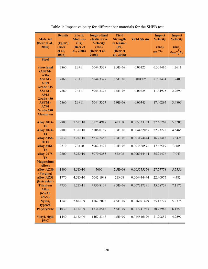
Table 1: Impact velocity for different bar materials for the SHPB test ...................... 20

Table 2: High Strain rate data for wet and dry polyurethane foam (Mathews, 2008) 29

Table 3: The test matrix .............................................................................................. 36

Table 4: Mechanical properties of foam sample ......................................................... 43

Table 5: Mechanical properties of foam + 1 side fine weave Kevlar ......................... 43

Table 6: Mechanical properties of foam + fine weave Kevlar on both sides ............. 44

Table 7: Mechanical properties of foam + 2x3 Kevlar on both sides ......................... 44

Table 8: Mechanical properties of fluid-filled foam + 2x3 Kevlar on both sides ...... 45

Table 9: Mechanical properties of fluid-filled foam + fine weave Kevlar on both sides

..................................................................................................................................... 45

Table 10: Mechanical properties of 6061-T6 Aluminum ........................................... 46

Table 11: The properties of the SHPB material at LANL .......................................... 49

Table 12: Comparison of the Theoretical and Experimental Data ............................. 61

vii    

LIST OF FIGURES

Figure 1: The schematic illustration of the SHPB test setup ........................................ 8

Figure 2: The SHPB in the laboratory at New Mexico Tech ........................................ 8

Figure 3: Teflon bushings and the pressure bars .......................................................... 9

Figure 4: Example of the incident, reflected and transmitted pulses. ......................... 11

Figure 5: Schematic of the sample-bar interface ....................................................... 12

Figure 6: The end-cap fitted onto the hollow aluminum output bar ........................... 25

Figure 7: The input and output bar signal for testing on the SHPB ............................ 26

Figure 8: The effect of strain rate on modulus (Mathews, 2008) ............................... 31

Figure 9: Comparison of previous (Mathews, 2008) and current (researcher) results of

strain rate on modulus ................................................................................................. 31

Figure 10: Sandwich composite of polyurethane foam and Kevlar ............................ 33

Figure 11: The different samples prepared for testing ................................................ 37

Figure 12: The SHPB apparatus at LANL (Courtesy of C. M. Cady) ........................ 39

Figure 13: The heating or cooling setup for controlled temperature testing (Courtesy

of C. M. Cady) ............................................................................................................ 40

Figure 14: Stress vs. Strain rate for different samples ................................................ 47

Figure 15: Modulus vs. Strain rate for the different sample tested ............................. 48

Figure 16: The stress-strain graph of polyurethane foam at room temperature .......... 50

Figure 17: Strain rate vs. strain at different temperature ............................................ 51

Figure 18: The stress-strain graph of polyurethane foam at 00 C ............................... 51

Figure 19: The stress-strain graph of polyurethane foam at -200 C ............................ 52

viii    

Figure 20: The stress-strain graph of polyurethane foam at -400 C ............................ 52

Figure 21: The stress-strain graph of polyurethane foam at -600 C ............................ 53

Figure 22: The stress-strain graph of polyurethane foam at -800 C ............................ 53

Figure 23: The stress-strain graph of polyurethane foam at -800 C ............................ 54

Figure 24: The stress-strain graph of polyurethane foam at -800 C ............................ 54

Figure 25: Stress-strain graph of polyurethane foam at different temperatures ......... 55

Figure 26: The effect of temperature on stress ........................................................... 56

Figure 27: Effect of temperature on modulus ............................................................. 57

Figure 28: The effect of temperature on strain rate .................................................... 57

Figure 29: Comparison of the theoretical and experimental data ............................... 59

Figure 30: Comparison of the theoretical and experimental data ............................... 60

Figure 31: Percent Error vs. Strain Rate ..................................................................... 62  

ix    

LIST OF ABBREVATIONS AND SYMBOLS

SHPB Split Hopkinson Pressure Bar

LANL Los Alamos National Laboratory

NMT New Mexico Institute of Mining and Technology

LED Light-emitting diode

C0 Elastic wave velocity

l0 Specimen length

E Young’s Modulus of output bar

A0 Cross sectional area of output bar

As Cross section of the specimen

ρ Density of the material

ε Strain

εt Strain in the output bar (transmitted strain)

εr Reflected strain in the input bar

εi Incident strain in the input bar

limpactor Impactor’s length

td Impact duration

dB Decibel

έ Strain rate

σ Stress

EMRTC Energetic Materials Research and Testing Center

1    

CHAPTER 1 INTRODUCTION

1.1. Motivation for Research  

The development of the new composite material resulted from a project

funded partly by the Office of Naval Research who was interested in a material for a

stealth naval platform. After an intense literature review about the characteristics of

different materials, researchers at New Mexico Institute of Mining and Technology

(NMT) decided that a multifunctional composite material could be developed. The

researchers chose quick-recovery polyurethane foam for a core layer and Kevlar for

skin layer to form a sandwiched composite (Ghosh et al., 2010). Dr. Ashok K. Ghosh,

the lead researcher, applied for patent and the U.S. Patent Office approved his

application and granted him patent for the composite material. Researchers carried

out various experiments to investigate the characteristics of this new material.

First, they (Ghosh, et al., 2007) examined its acoustic dampening

characteristics. The material revealed a 25 percent higher transmission loss than that

predicted by acoustic mass law at frequencies between 250 -1000 Hz. Further testing

at frequencies between 1 kHz and 10 kHz resulted in transmission loss as high as 135

decibel (dB) (Ghosh, et al., 2007). Researchers then investigated the thermal

properties of this composite material. The material demonstrated an induced

circulation due to convection (Ghosh et al., 2010). With these encouraging results,

researchers (Mathews, 2008, Ghosh et al., 2010) then decided to investigate the

material’s response to high strain rate loading. The work reported in this thesis is an

investigation to determine whether using the Split Hopkinson Pressure Bar (SHPB)

2    

apparatus, one of the most commonly used pieces of equipment for strain rates

between 102 s-1 and 104 s-1, can yield consistent, understandable data for

characterizing the material under question at high strain rates.

The effects of strain rate on material behavior are of significant importance to

researchers and engineers for the purpose of developing constitutive equations and

efficiently designing engineering structures that experience high strain rate loadings.

There are many different tests that have been develop over time to investigate strain

rate effects on material properties and limitations are dictated by the material under

investigation.

This research investigates the behavior of a low-mechanical impedance

material under high strain rate loading by utilizing the SHPB apparatus which

required modifications for obtaining valid experimental data since it was originally

designed for testing high strength materials. The theory of the SHPB is well

developed and researchers have been utilizing this tool for obtaining strain rate testing

between 102 s-1 and 104 s-1 with different materials exhibiting different behavior in

this strain rate regime. The polymer composite comprised of polyurethane foam and

Kevlar developed by researchers at New Mexico Tech is being investigated in this

study for its application in energy absorbing and shock isolation environments.

1.2. High Strain Rate Loading  

One of the most widely accepted methods of determining material stress-strain

characteristics at high strain rates is the SHPB apparatus (Harding, 1979). Bertram

Hopkinson conducted dynamic experiments in the early 1900 and discovered that the

3    

dynamic strength of steel is at least twice as high as its low-strain-rate strength. Steel

also undergoes a ductile-to-brittle transition when the strain rate is increased (Meyers,

1994). Consequently, researchers and engineers became interested in materials

behavior at varying strain rate. Meyers (1994) also agreed that it is important to test

different material because their responses vary greatly with strain rate. The new

foam-Kevlar composite developed by researchers at New Mexico Tech is expected to

exhibit an increase in strength with increasing strain rate. As mentioned previously,

foam is an example of a low mechanical impedance material, and these materials use

are increasing. Some known applications include protection in crashes and packaging,

among others (Chen et al., 2002).

1.3. Low Impedance Materials  

Engineering materials such as rubbers and foams are increasingly being used

in applications where they are subjected to high strain rate and deformations and as

shock and vibration absorbers. Some examples are crushable foams in vehicle

interiors for passenger protection during crashes, shock absorption application in

electronics packaging, and high performance body armors (Sharma et al., 2002, Chen

et al., 2000). These materials have low strength, low mechanical impedance, low

wave speed, and are often referred to as soft materials. They are typically good shock

mitigation and vibration isolation materials. For efficient engineering application and

design, the material response to impact loading needs to be determined through

vigorous research and experimentation (Song and Chen, 2004, Kolsky, 1949).

The objective of this research is to investigate the behavior of a low strength,

low mechanical impedance, quick-recovery polyurethane foam subjected to impact

4    

loading. The polyurethane foam is placed between two Kevlar-epoxy laminas,

forming a sandwiched composite material that aims to exploits the excellent shock

absorbing nature of polyurethane foam and the high tensile strength of Kevlar fibers.

Composite materials are widely used in today’s world and their areas of

application continue to expand. They include aerospace, aircraft, automotive, marine,

energy, infrastructure, armor, biomedical and recreational applications (Daniel and

Ishai, 2006). According to Daniel and Ishai (2006) composites have unique

advantages over monolithic materials: high strength, high stiffness, long fatigue life,

low density, and adaptability to the intended function of the structure. A thorough

understanding of this material’s response to applied loading conditions is necessary to

adequately design the material for specific applications. Therefore, the behavior of

this low mechanical impedance material to impact loading will be investigated

utilizing the split Hopkinson Pressure Bar apparatus. With the data obtained, an

attempt will be made to establish a framework for the development of a constitutive

equation to postulate the materials’ behavior under high strain rate loading conditions.

Constitutive equations are mathematical models that characterize individual

material and its response to applied loads under specific conditions. They consider the

macroscopic behavior resulting from the internal constitution of the material

(Malvern, 1969). The literature on this subject is vast and encompasses models for

solids and fluids, for elasticity, viscoelasticity, and plasticity, for Newtonian fluid and

non-Newtonian fluids, and others. Although the possibilities are endless, any

worthwhile constitutive model must be in reasonable agreement with physical

observation. Of considerable importance in this regard is the requirement that

5    

constitutive models satisfy the principle of material frame-indifference (Slaughter,

2002). Humphrey (2002) wrote numerous articles on constitutive relations, and

suggested that for the formulation of constitutive relations one must follow five basic

steps regardless of the approach; these are:

1. Delineate general characteristics of the material behavior,

2. Establish an appropriate theoretical framework,

3. Identify specific functional forms of the relations,

4. Calculate values of material parameters,

5. Evaluate the predictive capability of the final solutions.

A representation or description of the material behavior and characteristics

under the conditions of interest is needed to classify whether the material exhibits a

fluid-like or a solid-like response. If the response is dissipative, isotropic, isochoric, a

thorough understanding of all the characteristics of the material is essential so that the

appropriate constitutive relation can be formulated with this knowledge (Humphrey,

2002). Malvern (1969) emphasizes that it is not feasible to write down one equation

or a set of equations to describe accurately a real material over its range of behavior

because material behavior is very complex when the entire range of possible

temperatures and deformations are considered.

Investigating this composite’s response to impact loading will result in an

understanding of this new material’s behavior to determine if it can be used for

impact applications. The composite material is comprised of open-cell polyurethane

foam sandwiched on both sides by Kevlar fabric bounded together by epoxy resin and

6    

hardener. The investigation was carried out on the SHPB apparatus in the laboratory

at the New Mexico Institute of Mining and Technology. A brief introduction of the

classical SHPB apparatus, its limitations for testing low strength, low mechanical

impedance materials, the modifications necessary for different scenarios, and some

basic principles that must be followed for valid test results are briefly discussed in

Chapter 2.

7    

CHAPTER 2 LITERATURE REVIEW OF THE SHPB

2.1. The Split Hopkinson Pressure Bar Apparatus

Meyers (1994) states that the split-Hopkinson pressure bar (SHPB) is widely

accepted as the testing instrument for strain rates between the ranges of 102 to 104 s-1.

Also referred to as the Kolsky bar, it is the most extensively used experimental

configuration to measure the response of materials under high strain rate, and was

developed by Kolsky (Zukas, et al., 1982, Owens and Tippur, 2009, Lindholm and

Yeakley, 1968). The first person to investigate the propagation of stress pulses in a

laboratory scale was Bertram Hopkinson. His apparatus, known as the “Hopkinson

pressure bar”, consisted of a cylindrical steel bar several feet long, and approximately

an inch in diameter held in a horizontal position by four threads (Kolsky, 1963). Upon

impact from a projectile or subjecting the bar to contact with an explosive charge, a

compression pulse was produced and traveled down the bar. His system was “an

application of the simple theory of stress propagation of elastic pulses in a cylindrical

bar where the length of the pulse is great compared with the radius of the bar”

(Kolsky, 1963). When the diameter of the bar is small compared with the length of

the pulse, and the material of the bar is not stressed beyond its elastic proportional

limit, the pulse is not distorted as it travels down the length of the bar (Kolsky, 1949,

Kolsky, 1963).

The behavior of materials under high strain rate loading has been of interest

to engineers and researchers for the purpose of developing constitutive relations for

various materials (Sharma et al., 2002, Song and Chen, 2004, Kaisers, 1998, Kolsky,

1949). Figures 1 and 2 below illustrate the setup of the SHPB apparatus which

8    

consists of a gas gun, an impactor bar, an input bar and an output bar. Zukas et al.

(1982) recommended that the input and output bars be mounted on Teflon or nylon

bushings to assure accurate axial alignment while permitting stress waves to pass

without dispersion.

Figure 1: The schematic illustration of the SHPB test setup

Figure 2: The SHPB in the laboratory at New Mexico Tech

9    

It is also imperative for valid test data that the bars used are straight and free

to move without binding and accurately aligned. This accurate alignment is necessary

for uniform and one-dimensional wave propagation as well as producing uniaxial

compression within the specimen during loading. Restriction on bars’ movement will

lead to additional noise on the wave measured in the bars (Gray, 2000). The bars of

the SHPB apparatus used in the lab at New Mexico Tech are aligned on Teflon

bushings as shown in Figure 3, satisfying the alignment and one-dimensional wave

propagation criteria.

 

Figure 3: Teflon bushings and the pressure bars

The one-dimensional elastic wave is produced by the impacting bar which

strikes the input bar (incident bar) and creates an elastic pulse or longitudinal wave

which travels through the input bar, the sample under testing, and the output bar. The

incident pulse is measured by the strain gauge mounted on the incident bar. A pulse is

then reflected from the interface of the input bar and the sample which is again

measured by the strain gauge that is mounted on the incident bar. Thus, the strain

10    

gauge mounted on the incident bar measures both the incident εi (t) and the reflected

pulses εr (t) while the strain gauge on the output bar measures the transmitted strain εt

(t). Zukas et al. (1982) states that the equations for analyzing stress, strain, and strain

rate are based on the assumption that the stresses and velocities at the end of the

specimen are propagated down the bars in an un-dispersed manner. The wave-transit

time in the short specimen is small compared to the total time of the experiment and

many wave reflections can take place back and forth along the specimen. Also, the

stress and strain are assumed to be uniform along the specimen (Zukas et al., 1982).

When the incident bar is struck by the impacting bar, an elastic wave is produced, the

elastic wave deforms the specimen plastically. However, it is important to know that

the SHPB should not be considered as plastic wave propagation experiment (Meyers,

1994).

According to Kaiser (1998), the results of the Split-Hopkinson bar experiment

can be summarized as follows:

1. The reflected and transmitted waves are proportional to the specimen’s

strain rate and stress, respectively.

2. By integrating the strain rate generated from the test, the strain in the

sample can be determined and,

3. The stress strain properties can be calculated by analyzing the strain in the

input and output bars.

The longitudinal wave formed takes the shape shown in Figure 4. The shape

of the reflected and transmitted pulses are dependent on the area and mechanical

11    

behavior of the specimen, therefore, testing different materials or specimens will

produce pulses that have different shapes and sizes (Zukas et al., 1982).

 Figure 4: Example of the incident, reflected and transmitted pulses.

(http://www.tut.fi/index.cfm?MainSel=12870&Sel=13652&Show=18694&Siteid=142)

 

2.2. The Theory of the Split Hopkinson Pressure Bar  

According to Ninan et al. (2001), the displacement of the incident bar-sample

interface uI(t) is determined by εi (t) and εr (t), where

εi(t) = εI(t - ∆t) (1)

εr(t) = εI(t + ∆t) (2)

∆t is the time for the pulse to travel from the strain gauge on the input bar to the

sample, t is an instant in time, and εI is the strain recorded by the strain gauge in the

incident bar at any instant t in time. The strain in the output bar is given by εt and εr is

the strain in the input bar. The displacement u1 of the input bar and the sample

interface is given by Equation (3). Equation (4) gives the displacement at the sample

and output bar interface u2 given by Zukas et al. (1982).

 

12    

u1 =C0 (  −𝜀! +  𝜀!)!! 𝑑𝑡                                                                                                                        (3)

u2 = -C0 𝜀!!! 𝑑𝑡                                                                                                                                (4)

Where C0 is the longitudinal wave velocity of the bar. The average strain in the

sample is given by:

εs = !!!  !!!!

= !!!!

−𝜀! +  𝜀! −  𝜀! 𝑑𝑡!! (5)

Where l0 is the length of the specimen. The load at the sample interface P1 and P2

described by Ninan et al. (2001), and shown in Figure 5, can be determined from the

folowing equations:

P1 = AsE (εi + εr) (6)

P2 = AsEεt (7)

Where As is the area of the specimen and E is the elastic modulus of the pressure

bars.

 

Figure 5: Schematic of the sample-bar interface

 

Assuming that the pressure difference at each interface of the sample is negligible,

then according to Graff (1991), εt  = εi - εr and substituting this into Equation (5) gives:

εs(t) = - !!!!!

𝜀!𝑑𝑡!! (8)

13    

which represents the sample average strain. The stress can be obtained directly from

the transmitted strain as given in Equation (9). The strain rate in the speciment is

given by Equation (10).

σs = E!!!!εt (9)

έs = !!!!!!εr (10)

Where

A0 is the cross sectional area of the output bar

As is the cross sectional area of the specimen

σs is the stress in the specimen

έs is the strain rate of the specimen

Graff (1991) also stated that in practice, the sample average strain can be obtained by

directly integrating the reflected strain and the stress can be obtained directly from the

transmitted strain. The stress, strain, and strain rate are average values, and they are

determined by assuming uniaxial stress state in the specimen (Zukas et al., 1982).

Traditionally, the SHPB is used to investigate material behavior under

dynamic loading conditions. It is commonly used for testing metals, concrete, and

ceramics (Chen, et al., 2000). The Split Hopkinson pressure bar can also be used to

test composite materials. According to Ninan et al. (2001) there has been a few but

relatively recent attempts to systematically model the rate-dependent deformation of

composite laminates beyond the elastic region.

14    

This apparatus can also be used to investigate behavior of low strength, low

mechanical impedance materials. However, the proper modifications are necessary to

obtain reliable data.

2.3. Modifications on the SHPB Apparatus for Testing Low Strength, Low Mechanical Impedance Materials  

With a few adjustments, the SHPB can also be used to determine high strain

rate behavior of low mechanical impedance materials. With these materials, the

incident bar-specimen interface moves almost freely under stress wave loading

because most of the incident pulse is reflected back into the incident bar and a very

small signal is transferred to the transmission bar (Chen et al., 1999). One method

proposed for increasing the signal strength is using a hollow transmission bar (Chen

et al., 1999). An X-cut quartz crystal disk embedded in a solid transmission bar

(Chen et al., 2000) is also another method of obtaining an amplified transmitted

signal. Pulse shaping technique is also another modification (Johnson et al., 2009).

2.3.1. Embedded Quartz Crystal  

Chen et al. (2000) suggested that, for increasing the signal in the transmission

bar when testing low mechanical impedance materials a circular piezoelectric

transducer (an X-cut quartz crystal disk) should be embedded in the middle of a

solid aluminum transmission bar of the same diameter to directly measure the

time-resolved transmitted force. The X-cut quartz is much more sensitive in

detecting forces in its x-direction than the indirect surface strain gauge method. The

mechanical impedance of the self-generating quartz transducer is also very close

to the mechanical impedance of the aluminum transmission bar. This ensures that

15    

introduction of the quartz disk does not affect the one-dimensional wave propagation

in the transmission bar (Chen, et al. 2000).

2.3.2. Hollow Transmission Bar  

Researchers at the University of Arizona (Chen et al., 1999) have proposed

other modifications for the testing of low mechanical impedance materials. They

suggested that a high-strength aluminum alloy should be used for the incident bar and

a hollow aluminum tube should be used for the transmission bar. The hollow

aluminum tube will cause an increase in σs according to Equation (9). Also, the

hollow tube will produce an increase in the transmitted signal amplitude (Chen et al.,

1999). The SHPB apparatus in our experiment utilizes 6061-T6 aluminum bars; one

hollow transmission bar and one solid incident bar. The transmission bar has an outer

diameter of 31.78 mm and is 6.35 mm thick. The solid incident bar has a 31.75 mm

diameter.

Although the principles are the same when using solid or hollow pressure

bars, the theory for determining the strain in the specimen when using hollow bars is

different. Chen et al. (1999) developed an equation for determining the strain for low

impedance materials using hollow transmission bars. They suggested that according

to Equation (9), the stress is a function of the transmitted stain εt(t) and therefore in

order to increase εt(t) under the same stress level either the area of the output bar A0

or the Modulus E should be reduced. Using a hollow bar will result in a smaller A0

and using low impedance bar material with a lower elastic modulus will cause an

increase in the transmitted stain εt(t). The hollow bar must be fitted (press fitted) on

16    

the end with a cap of the same bar material at the bar-specimen interface (Chen et al.,

1999). From intuition, one might believe that the end cap will interfere with the stress

pulse passing through the bar. However, the researchers (Chen et al., 1999) stated that

using a pulse shaper to obtain a significant increase in the rise time of the loading

pulse and filtering out high-frequency components in the waveform, the effect of the

end cap can be neglected. Pulse shaping techniques will be discussed in Section 2.3.3.

Chen, et al. (1999) stated that by using a hollow aluminum bar of 19 mm outer

diameter and 1.5 mm wall thickness, the transmitted signal is amplified 10 times as

compared to using solid steel bars. This is from the combined effect of the lower

Elastic modulus and the ratio of A0/As of the hollow aluminum bar.

To further increase the amplitude of the transmitted signal, transmission bars

with thinner walls can be used. Chen et al. (1999) also proposed a modification of the

theory to determine the strain in the specimen. When the specimen is in equilibrium,

Equations (6) and (7) are equal, and yield

εt = !!!!(𝜀! + 𝜀!) (11)

Where Ai and At are the cross-sectional areas of the incident and transmission bars

respectively, and substituting equation (11) into equation (5) gives the strain in the

specimen as

εs = !!!!

1−   !!!!

𝜀! 𝑡 𝑑𝑡 −  !!!!

!! 1+   !!

!!𝜀!  

!! 𝑡 𝑑𝑡 (12)

Equation (12) is used to calculate the strain in the specimen from the measured

incident and reflected pulses when a hollow transmission bar is used. This equation is

17    

quite different from Equation (8) which is used in the classical SHPB test with bars of

same cross-sectional areas (Chen et al., 1999).

2.3.3. Pulse Shaping  

Pulse shaping technique is another approach that is used to facilitate the

testing of low impedance materials (Johnson et al., 2009). It is used to produce a

slowly raising incident pulse, which is necessary to minimize the effect of dispersion

of the wave in the bars and to allow the sample to achieve dynamic stress equilibrium

(Frew et al., 2005) which is necessary in SHPB testing (Song and Chen, 2004). For

dynamic stress equilibrium, the loading pulse must stress the front and the back faces

of the specimen almost simultaneously. In testing soft materials, this can be achieved

by pulse shaping (Chen et al., 1999). The incident pulse can be shaped by two

methods, by machining a larger radius on the impactor face or by placing a tip

material between the input bar and the impactor which can be made of any material

such as aluminum, brass, paper, or stainless steel, in the shape of a disk slightly larger

than the bars (Frew et al., 2005). A nearly constant strain rate in a sample can be

generated by choosing the proper pulse shaper (Chen et al., 1999, Frew et al., 2005).

The pulse shaping technique is used to decrease the initial incident loading rate by

increasing the rise time of the incident pulse (Song and Chen, 2005).

A simple pulse shaping technique for testing low impedance materials

involves attaching a polymer disk with a thin layer of vacuum grease to the impact

end of the incident bar. The polymer disk will deform plastically upon impact and

effectively increase the rise time of the pulse (Chen et al., 1999). Also, on the impact

surface of the polymer disk, attaching two layers of tissue paper using vacuum grease

18    

will filter out high-frequency components in the incident pulse (Chen et al., 1999).

This method was used in this investigation because it was found to be effective for

this new material; previous researchers have utilized this technique with great success

(Mathews, 2008).

The amplitude and duration of the incident pulse can be controlled by varying

the striker bar velocity and length, respectively (Chen et al., 1999). According to

Meyers (1994), the impact duration td is determined from the following equation:

𝑡!!  !!!"#$%&'(  !!

(13)

Where limpactor is the impactor length and C0 is the elastic wave velocity. This equation

is valid only if the impactor and the input bars are of the same materials. So from

Equation (13), the duration of the incident pulse can be increased by increasing the

length of the impactor. The amplitude of the incident pulse is directly related to the

impactor velocity since it produces the compressive wave in the input bar. The

particle velocity Up is parallel to the wave velocity for longitudinal wave, as in the

SHPB. The stress in the input bar is given by the equation below (Meyers, 1994).

𝜎 =  𝜌  𝐶!𝑈! (14)

Equation (14) can then be used to determine the maximum impact velocity.

Since the SHPB apparatus involves the propagation of an elastic pulse through the

bars, the pulse transmitted to the input bar should have an amplitude not exceeding

the elastic limit. Using Hooke’s Law, the strain in the bar is given by

𝜀 =   !! (15)

19    

Since we are interested in keeping the bars in the elastic region, then the

maximum impact velocity Up can be determined by

𝑈! =  !  !!"#!  !!

(16)

where εmax is 1/5 εy.

Table 1 below was developed by the researcher using materials properties by

Beer et al. (2006) to serve as a guide for the maximum impact velocity for different

bars and impactor materials for the SHPB test. The bar material can vary depending

on the different samples or specimen material being investigated. It is important that

the impact doesn’t yield the bar material; if the impact velocity causes the bar

material to yield then it will cause the propagation of elastic and plastic waves. Plastic

waves of uniaxial stress in bars or rods are dispersive in nature and they attenuate as

they propagate down the bar; if the bars remain elastic, then the pulse is propagated

undistorted (Zukas et al., 1982). The stress is always much less than the elastic

modulus under elastic conditions, therefore, the particle velocity Up will be very small

compared with the longitudinal wave velocity C0 (Graff, 1991).

20    

Table 1: Impact velocity for different bar materials for the SHPB test

Material

(Beer et al., 2006)

Density

(kg/m3) (Beer et al., 2006)

Elastic Modulus

(Pa) (Beer et

al., 2006)

longitudinal elastic wave

Velocity (m/s)

(Beer et al., 2006)

Yield Strength in tension

(Pa) (Beer et

al., 2006)

Yield Strain

Impact Velocity

(m/s)

max =εy

Impact Velocity

(m/s)

εmax=𝟏𝟓𝜺𝒚

Steel

Structural (ASTM-

A36)

7860 2E+11 5044.3327 2.5E+08 0.00125 6.305416 1.2611

ASTM - A709

Grade 345

7860 2E+11 5044.3327 3.5E+08 0.001725 8.701474 1.7403

ASTM - A913

Grade 450

7860 2E+11 5044.3327 4.5E+08 0.00225 11.34975 2.2699

ASTM - A790

Grade 690

7860 2E+11 5044.3327 6.9E+08 0.00345 17.40295 3.4806

Aluminum

Alloy 2014-T6

2800 7.5E+10 5175.4917 4E+08 0.005333333 27.60262 5.5205

Alloy 2024-T4

2800 7.3E+10 5106.0189 3.3E+08 0.004452055 22.73228 4.5465

Alloy-5456-H116

2630 7.2E+10 5232.2486 2.3E+08 0.003194444 16.71413 3.3428

Alloy-6061-T6

2710 7E+10 5082.3477 2.4E+08 0.003428571 17.42519 3.485

Alloy-7075-T6

2800 7.2E+10 5070.9255 5E+08 0.006944444 35.21476 7.043

Magnesium Alloys

Alloy AZ80 (Forging)

1800 4.5E+10 5000 2.5E+08 0.005555556 27.77778 5.5556

Alloy AZ31 (Extrusion)

1770 4.5E+10 5042.1948 2E+08 0.004444444 22.40975 4.482

Titanium Alloy

(6%Al, 4%V)

4730 1.2E+11 4930.8109 8.3E+08 0.007217391 35.58759 7.1175

Nylon, type6/6

1140 2.8E+09 1567.2078 4.5E+07 0.016071429 25.18727 5.0375

Polystyrene 1030 3.1E+09 1734.8512 5.5E+07 0.017741935 30.77962 6.1559

Vinyl, rigid PVC

1440 3.1E+09 1467.2347 4.5E+07 0.014516129 21.29857 4.2597

21    

The selection of bars for the SHPB testing depends on a number of criteria.

For example, for metals, the classical SHPB apparatus can be utilized while low

impedance, low strength specimens can be tested with hollow bars. However, it is

important that the length and diameter of the bar be chosen so that valid results,

maximum strain rates, and strain levels are obtained. The lengths of the bars need to

be chosen carefully so that they will ensure one-dimensional wave propagation for a

given pulse length. For most material testing, this propagation requires the bar length

to be approximately 10 bar diameters (Gray, 2000). But to readily allow separation of

the incident and reflected pulse for data reduction, the bars should have length-to-

diameter ratio (L/D) exceeding 20 (Gray, 2000). According to Gray (2000) the

selection of the bar diameter will influence the maximum strain rate obtained from

testing because the highest strain rate requires the smallest bar diameter. Another

consideration for selecting the appropriate bar length is the amount of strain in the

specimen that is needed by the researcher. The magnitude of the strain is related to

the length of the incident pulse, requiring that the incident bar be at least twice the

length of the incident pulse to prevent interference between the incident and the

reflected pulses (Gray, 2000, Meyers, 1994).

Sample thickness is another important factor to be considered when testing on

the SHPB system, especially on low strength, low impedance materials (Chen et al.,

2000). One important requirement of the SHPB theory is that the specimen

undergoes homogeneous deformation.

The SHPB experiments can also be performed at different temperatures.

Researchers at Los Alamos National Laboratory have the SHPB equipment designed

22    

to carry out experiments between -100 0F and 1700 F (Gray and Blumenthal, 2000).

Researchers have found that due to the low mechanical impedance of polymers, the

signals into the pressure bars are small and sometimes non-detectable by the strain

gauges affixed to them during experiments on some polymers (Gray and Blumenthal,

2000). Testing polymers at lower temperatures produces detectable signals and gives

a better understanding of these polymers at high strain rate loading. With decreasing

temperatures, the yield and flow stresses and yield strain increase (Siviour et al.,

2005). For this reason, some tests were carried out between 0 0C and -80 0C at Los

Alamos National Laboratory.

The literature for SHPB testing is immense with researchers making various

modifications for testing different materials. The general principles are similar for

most of the cases, and test results are valid when the correct modifications are made.

Based on the literature review, some modifications have been made on the SHPB at

the NMT laboratory. These modifications and the tests completed will be discussed in

the following Chapters 3 and 4.

23    

CHAPTER 3 DESCRIPTION OF THE SHPB

3.1. The Split Hopkinson Pressure Bar Apparatus in the Laboratory at New

Mexico Tech

The investigation of material behavior under high strain rate has been an area

of interest for engineers and researchers for the purpose of better understanding

material behavior and developing constitutive equations for predicting or modeling

their behavior to impact loading environments (Song and Chen, 2004). At the New

Mexico Institute of Mining and Technology (NMT), student researchers are given an

opportunity to investigate material behavior under high strain rate using a SHPB

apparatus. This apparatus will be described briefly in this chapter and prior testing

carried out by previous student researchers on the SHPB will be analyzed.

The SHPB apparatus in the NMT lab was designed and developed by the

mechanical engineering students and was modified and updated by Dr. Ashok Kumar

Ghosh; his contribution and enthusiasm in impact loading behavior of material made

it possible for students to be able to utilize the apparatus for high strain-rate

investigations. The SHPB consists of an input bar, an output bar and an impactor. An

actuated ball valve releases air that is stored in a tank generated by an air compressor.

The air launches the impactor causing it to strike the input bar. The strains measured

by the strain gauges are recorded by a LABVIEW data acquisition system and

analyzed using DIADEM analysis software.

24    

3.2. The Components of the SHPB Apparatus

3.2.1. The Air Compressor and Reservoir  

The air is supplied by a 1.8 hp, 200 psi DeWALT electric air compressor. The

compressed air is released into a reservoir by relief valves. There are two relief

valves; one releases the air to the reservoir and the other pressurizes the actuated ball

valve for propelling the impactor. A pressure gauge measures the air pressure in the

reservoir. This allows for the precise control of the reservoir pressure, on which the

impact velocity is dependent. As the pressure in the reservoir is increased, the

impactor velocity will be increased therefore allowing the researchers to control and

vary the impact velocity for specific impactor material and length. The reservoir used

in this system is a propane tank that has been modified for the SHPB apparatus. The

reservoir delivers air directly to the impactor bar which is housed in a 50.8 mm pipe,

projecting it towards the input bar. The pipe is fitted with an air actuated ball value at

the end of the reservoir. The compressor provides air that triggers the opening of the

ball valve through a circuit relay that can be activated by the researcher; the air

actuated ball valve requires a pressure of 80 psi for activation and provides the best

means of releasing the air from the reservoir instantaneously for launching the

impactor. At the end of the impactor barrel, two light-emitting diodes (LEDs) and two

SFH 314 sensors are affixed.

These LEDs and sensors provide a means of measuring the projectile/impactor

velocity for different reservoir pressures. For different impactor lengths, diameters,

and materials, the LEDs and sensors can be utilized to calibrate pressure against

velocity. This calibration is an important aspect since it allows researchers to

25    

investigate the relationship of impact velocity and strain rate, and also to ensure that

the impactor velocity does not exceed the maximum particle velocity Up to cause

yielding in the input bar. Table 1 lists some typical bar materials and the maximum

impact velocity that can be achieved on the SHPB system.

3.2.2. The Input and Output Bars  

Aluminum 6061-T6 input and output bars are used for the testing of the low

impedance composite material. The input and output bars are 1.2192 m long and

31.75 mm in diameter. The output bar is hollow with an internal diameter of 19.05

mm and press fitted with an aluminum end cap shown in Figure 6.

 

 

Figure 6: The end-cap fitted onto the hollow aluminum output bar

26    

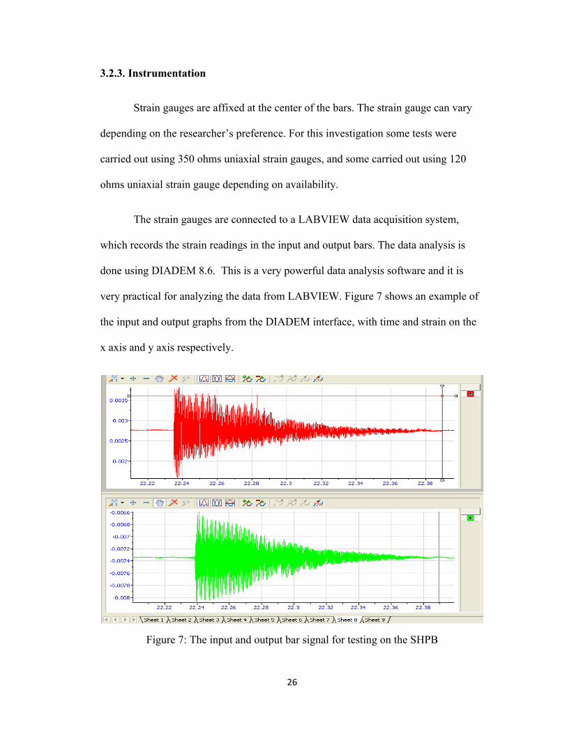
3.2.3. Instrumentation  

Strain gauges are affixed at the center of the bars. The strain gauge can vary

depending on the researcher’s preference. For this investigation some tests were

carried out using 350 ohms uniaxial strain gauges, and some carried out using 120

ohms uniaxial strain gauge depending on availability.

The strain gauges are connected to a LABVIEW data acquisition system,

which records the strain readings in the input and output bars. The data analysis is

done using DIADEM 8.6. This is a very powerful data analysis software and it is

very practical for analyzing the data from LABVIEW. Figure 7 shows an example of

the input and output graphs from the DIADEM interface, with time and strain on the

x axis and y axis respectively.

 

Figure 7: The input and output bar signal for testing on the SHPB

27    

3.3. Tests Conducted by Previous Researchers  

The SHPB apparatus has been used by students at the New Mexico Institute of

Mining and Technology to investigate the response of materials at high strain rate

loading. Jason Matthews (2008), a former graduate student at New Mexico Tech,

investigated the response of polyurethane foam to impact loading using the SHPB.

The result of his findings is summarized below.

Polyurethane foam is referred to as a material with low mechanical

impedance and low strength (Song and Chen, 2004). Modifications are necessary to

successfully utilize the SHPB apparatus for obtaining valid test data when testing soft

materials. Some modifications were made by previous researchers for testing the

polyurethane foam at the New Mexico Institute of Mining and Technology

laboratory. These modifications include replacing the steel bars with aluminum bars;

a solid input bar a hollow output aluminum bar as recommended by Chen et al.

(1999). With these modifications, some tests were carried out on the polyurethane

foam, some on wet samples (fluid filled) and some on dry samples. The foam samples

were 12.7 mm thick.

The results obtained by Mathews (2008) reveal that the samples with water in

the pores of the polyurethane foam have a higher modulus than the dry samples, and

as the strain rate increased the modulus also increased. His experiments were carried

out at breech pressures of 10 psi and 15 psi. These correspond to strain rates of 1088

s-1 and 2437 s-1 for dry foam and 1537 s-1 and 1669 s-1 for wet foam (Mathews, 2008).

According to Mathews (2008) the dry samples have a slower strain rate at 10 psi and,

28    

as the pressure increased, the wet samples showed a slower strain rate. At 20 psi, all

the samples exhibited signs of failure. Mathews (2008) stated that graphical

representation of the data showed that the dry samples had a lower modulus than the

wet samples at the same strain rate. The wet samples underwent less deflection than

the dry samples; they displayed 10 times the modulus of the dry samples with only

75% of the strain (Mathews, 2008). The fluid in the foam is pushed into empty pores

upon impact and thereby absorbing the impact energy more effectively than the foam

alone. Table 2 below is a summary of Mathews’s work on the SHPB with the wet and

dry foam samples (Mathews, 2008).

29    

Table 2: High Strain rate data for wet and dry polyurethane foam (Mathews, 2008)

Test # Sample Condition

Modulus (MPa)

Strain Rate (s-1)

Tank Pressure

1 dry 2.25 1088 10

2 dry 2.53 1101 10

3 dry 2.33 1078 10

4 dry 2.84 1086 10

5 dry 2.13 1088 10

6 wet 132 1538 10

7 wet 130 1523 10

8 wet 128 1532 10

9 wet 134 1567 10

10 wet 133 1525 10

11 dry 21.3 2341 15

12 dry 148 1687 20

13 dry 20.9 2461 15

14 dry 22.6 2511 15

15 dry 19.8 2437 15

16 wet 332 1687 15

17 wet 583 1937 20

18 wet 327 1701 15

19 wet 341 1665 15

20 wet 311 1623 15

30    

The preliminary data for the foam samples obtained by Mathews (2008) as

shown in Table 2 above was plotted in Figure 8. It shows a dramatic increase in the

modulus of the fluid filled samples compared to the increase in the modulus of the

dry samples. Figure 9 compared the data of foam samples obtained by Mathews

(2008) and the author. “JM” represents Mathews’s data and “NB” represents the

author’s data. The difference between these sets of data is noticeable.

Two factors that may have contributed to these differences are sample size

and temperature of testing. Mathews (2008) placed the foam specimen in a sample

holder between the input and out bars, with the specimen larger than the bar diameter.

The author however, sandwiched specimen of 25.4 mm diameter directly between the

input and output bars. According to Gray (2000) specimen should be 80% of the bar

diameter to allow for 30% strain before the specimen exceeds the bar diameter. The

temperature of testing environment may also be a contributing factor. According to

Siviour et al. (2005) the mechanical properties of polymers are effect by temperature.

Since the testing was done in a warehouse at different seasons, temperature could

have influenced the results.

Most of Mathews (2008) experiments were carried out under blast loading at

EMRTC. He subjected the foam samples to explosive charge and recorded their

behavior. The reader is encouraged to review his work for an in-depth discussion of

the foam’s behavior under blast loading.

31    

 

Figure 8: The effect of strain rate on modulus (Mathews, 2008)

 

 

 

Figure 9: Comparison of previous (Mathews, 2008) and current (researcher) results of strain rate on modulus

0  

50  

100  

150  

200  

250  

300  

350  

400  

0   500   1000   1500   2000   2500   3000  

Mod

ulus  (M

Pa)  

Strain  rate(s-­‐1)  

Modulus  vs  Strain  rate  

dry  foam  

fluid  filled  

0  

50  

100  

150  

200  

250  

300  

350  

0   500   1000   1500   2000   2500   3000  

Mod

ulus  (M

Pa)  

Strain  rate  (s-­‐1)  

Modulus  vs  Strain  rate  

JM  dry  

NB  dry  

JM  fluid  filled  

NB  fluid  filled  

32    

These preliminary results seem promising and therefore further investigations

were carried out with the same polyurethane foam. However, the foam was

sandwiched by Kevlar skin layers and subjected to impact loading. Kevlar was

selected after an intense literature review for a suitable skin layer. Many different

fabrics that were thoroughly researched for the skin layers include carbon fiber,

Kevlar, Nomex, fiberglass, and ballistic nylon (Ghosh et al. 2010). Kevlar find

applications in bulletproof vests, puncture resistant vests, needle resistant gloves,

helmets, and kayaks. There are different grades of Kevlar such as Kevlar 29, 49, and

149 with the greater number indicating a higher tensile modulus, but a lower tensile

elongation. Generally, this fabric is very strong for its weight with a high modulus

and high flexibility. It is also fire resistant and will not combust, but only degrade at

high temperatures (800° to 900°F) (Ghosh et al. 2010).

 3.4. Sample Preparation  

For reliable data, care must be taken in preparing samples for testing on the

SHPB apparatus. There are some basic requirements that must be met for samples

that are to be tested on the SHPB apparatus. These include:

1. The faces of the samples must be flat so that excellent contact can be

established with the pressure bars and the sides must be orthogonal to the loading

surface for uniform elastic loading (Gray, 2000).

2. When preparing samples for testing on the SHPB, the thickness is the

dominant factor for consideration for a given sample diameter because it affects the

33    

dynamic stress equilibrium process; a fundamental requirement of the SHPB analysis

(Song and Chen, 2004, Gray, 2000). These requirements were considered and

satisfied while preparing samples for this investigation. Precaution was taken during

the manufacturing of the composite samples for testing to ensure that all samples

were made appropriately.

The composite material was prepared using polyurethane foam and Kevlar.

The foam and Kevlar were bonded with MAS epoxy resin and hardener to produce a

sandwiched composite material with the foam on the inside. The figure below is an

example of the sandwich polyurethane foam composite.

Tests were also carried out on samples which had the pores of the foam filled

with fluid (wet samples). Filling the foam with fluid was done after the composite

materials had been constructed. As discussed earlier, test results obtained by

Mathews (2008) revealed that fluid in the pores of the polyurethane foam produced a

Figure 10: Sandwich composite of polyurethane foam and Kevlar

34    

material with promising shock absorbing properties. Modifications to rectify some of

the deficiencies of axial alignment and reliable pressure measurements with the

previous SHPB apparatus were made and additional experiments were conducted to

further investigate this material’s behavior to impact loading.

3.5. Modifications of the SHPB for Current Testing  

Some of these modifications include affixing a pressure gauge to the reservoir

to more precisely measure the tank pressure and create a more user friendly operating

system. Previously, the reservoir pressure was measured using a pressure transducer

that required the usage of a voltmeter to measure voltage and correlate the readings to

pressure. This was a time consuming process which created the introduction of

human error; with the dial pressure gauge, measurements were quick and accurate.

To further increase the alignment of the pressure bars, additional supports

were installed onto the system. According to Zukas et al., (1982) precise alignment of

the pressure bars is crucial. Additional supports made of aluminum and Teflon

bushings were installed to allow the stress wave to pass without dispersion. Some fine

adjustments were made to further align the bars precisely (optimal axial alignment),

these include readjusting the existing supports which were found to be slightly

misaligned and cleaning of the barrel to allow the impactor to travel unimpeded

towards the input bar. Also, the input and output bars were sanded so that they are

smoother and can move without restraint; one important requirement according to

Gray (2000). A new end cap was also made and fitted onto the hollow output bar.

When using a hollow output bar, the end cap should be press fitted onto the end of the

35    

bar, it should fit firmly (Chen et al., 1999). The old cap was fitted snugly which could

be a source of error.

The completed modifications made the system more efficient and testing

could be conducted. The experiments were conducted between 5 psi and 15 psi tank

pressure range. The testing procedure will be discussed in Chapter 4.

36    

CHAPTER 4 TESTS CONDUCTED

4.1. Test Matrix  

Many different samples were made according to the test matrix shown in

Table 3 below and were tested under the standard test procedure of the SHPB

apparatus at various breech pressures. The preparation of the different samples and

sample testing are discussed in this chapter.

Table 3: The test matrix

Impact pressure (psi) Sample description

5

A, B, C, D

10

15

Sample description:

A: foam only

B: foam + 779 Kevlar (one face only)

C: foam + 779 Kevlar (both faces)

D: foam + 2 x3 Kevlar on both faces

The total mass of a 101.6 mm square sample with one layer of Kevlar on both sides is

approximately 45 grams. The mass of each component is as follows:

Mass of 101.6 mm square 2x3 Kevlar = 3.73 g

Mass of 101.6 mm square fine weave Kevlar = 1. 38 g

Mass of 101.6 mm square polyurethane foam = 31.69 g

Mass of MAS epoxy resin and hardener for 101.6 mm square sample = 7.5 g

37    

The foam material used is open cell quick recovery polyurethane foam of 25.4

diameter and 12.7 mm thickness. The density of the foam material is 15 lb/ft3 and its

tensile strength of 40 psi (Rogers Corporation, 2010)

 

The composite samples were prepared according to the matrix in Table 3. The

basic materials used were quick-recovery polyurethane foam, Kevlar fibers, and

epoxy-resin. A detailed explanation of the composite sample preparation will not be

discussed because it involves patented information. The different samples prepared

are shown in Figure 11 below.

Figure 11: The different samples prepared for testing

38    

4.2. Test Procedure  

1. The different composite samples were prepared.

2. Foam samples were cut to the required size using a coring tool. The composite

samples were cut using a band saw. After the samples were cut to the desired

dimension they were tested under impact loading.

3. For testing, the sample was sandwiched between the bars and a small amount

of vacuum grease was applied to the sample ends of the input and output bars

to keep the sample in position and avoid any effects of friction, according to

Chen et al. (2000) petroleum jelly is also effective.

4. The striker bar (impactor) was pushed back into the barrel towards the

actuated ball valve on the reservoir so that upon the opening of the valve, the

air pressure will propel the striker bar forward and produce the impact on the

input bar.

5. The air compressor was used to pressurize the reservoir to the desired pressure

for the different impact velocities.

6. After pressurizing the reservoir, LabView VI was opened.

7. The actuated ball valve connected to the reservoir was activated and the

projectile launched, producing an impact in the input bar, which propagated

through the sample and the output bar.

8. The strain gauges on the input and output bars were used to record the strain

caused by the impact and the data was analyzed.

39    

Steps 2 – 7 were repeated for all the different samples to generate the data needed for

this report. Tests were also carried out at Los Alamos National Laboratory and these

data were compared to those obtained in the lab at NMT.

4.3. Experiments Conducted at LANL  

Experiments were also conducted at Los Alamos National Laboratory on the

SHPB apparatus at temperatures between 00C and -800C using solid magnesium

pressure bars of 9.525 mm diameter. The input and output bars were 762 mm long

while the striker bar was 152.4 mm long. Figure 12 shows the SHPB at Los Alamos

National Laboratory. The researchers at Los Alamos National Laboratory can conduct

experiments on their SHPB apparatus over a range of temperatures.

 

Figure 12: The SHPB apparatus at LANL (Courtesy of C. M. Cady)

 

Researchers at LANL are conducting high strain rate testing on materials

between -100 and 1700 F (Gray et al., 2000). The samples can be cooled or heated

depending on the testing data desired. According to Gray et al. (2000) cooling and

40    

heating of samples is done by Helium gas within a stainless steel containment

chamber at partial vacuum. By passing helium through a copper coil positioned

within liquid nitrogen dewar, cooling of the helium gas below ambient temperature is

obtained; while heating the helium in a parallel coil within a glycerin-filled beaker

warmed by a heating plate produce heated samples (Gray et al. 2000). Figure 13

shows the heating and cooling setup for controlled temperature testing on the SHPB

apparatus at Los Alamos National Laboratory. A thermocouple positioned to lightly

touch the outside of the sample is used to monitor the temperature of the sample. The

flow rate of the helium gas around the manifolds can be controlled to adjust/regulate

the temperature of the sample (Gray et al., 2000).

 

Figure 13: The heating or cooling setup for controlled temperature testing (Courtesy of C. M. Cady)

 

41    

The advantage of testing at lower temperature (below 770 F) for a range of

polymers show that both the measured loading elastic modulus and the measured

peak flow stress increases with decrease temperature (Kukureka and Hutchings, 1984,

Walley et al., 1991). Also, the behavior of polymers and polymer composites for

temperatures between -40 0C and 40 0C are relevant for arctic to desert environments

(Gray et al., 2000).

Polyurethane foam samples were tested between 0 0C and -80 0C at Los

Alamos National Laboratory. The samples were 7.9375 mm in diameter and 4.7625

mm in length. The data obtained from these tests are used to formulate a simple

relationship between strain rate and modulus for the polyurethane foam that has been

used as the core layer for the composite material.

 

   

42    

CHAPTER 5 RESULTS AND DISCUSSION  

Modifications were made to the conventional SHPB to investigate the impact

response of a composite material consisting of polyurethane foam and Kevlar. The

steel bars of the SHPB apparatus were replaced with aluminum rods to cater to the

impedance mismatch of the very low mechanical impedance foam material. A hollow

aluminum tube was used for the output bar to produce a magnified signal of the

transmitted pulse. According to many researchers, the low impedance material causes

most of the incident pulse to be reflected back into the incident bar, resulting in a very

low transmitted signal through the specimen (Chen et al., 1999). Test results of the

composite material confirm this observation. During the analysis of the strain

measurement from the input and output bars, the difference between the strain

measurements (signal amplitude) was considerable.

 

5.1. Tests Completed at NMT Laboratory  

The foam and different composite samples were tested on the SHPB

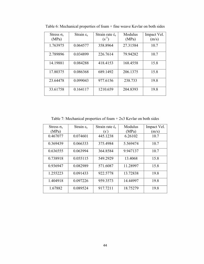
apparatus. Tables 4 – 9 show the values of stress, strain and strain rate obtained from

the experiments. These results show that with increasing velocities, the stresses,

strains and the strain rates increased. The stress and strain values were used to

determine the average dynamic modulus of the foam and composites. As expected,

the dynamic modulus of the foam and composite samples increased with increasing

strain rate. Also, the fluid filled composites exhibited an increase in dynamic modulus

when compared to the dry samples.

 

43    

Table 4: Mechanical properties of foam sample

Stress σs (MPa)

Strain εs Strain rate έs (s-1)

Modulus (MPa)

Impact Vel. (m/s)

10.75393 0.05395 537.6173 199.3331 10.7

10.38436 0.048235 495.2771 215.2876 10.7

26.05064 0.13312 1416.569 195.6926 15.8

26.43303 0.13597 1356.6 194.4041 15.8

24.31467 0.130893 1322.281 185.7599 15.8

30.96925 0.133597 1328.457 231.8106 19.8

41.67875 0.143285 1433.401 290.8795 19.8

Table 5: Mechanical properties of foam + 1 side fine weave Kevlar

Stress σs (MPa)

Strain εs Strain Rate έs (s-1)

Modulus (MPa)

Impact Vel. (m/s)

9.647455 0.101541 1014.973 95.01058 10.7

11.10345 0.10207 1032.915 108.7826 10.7

18.77432 0.113477 1140.833 165.4468 15.8

13.40576 0.119542 779.7041 112.1424 15.8

20.04733 0.18639 1839.758 107.5557 19.8

21.64255 0.157143 1562.798 137.7248 19.8

44    

Table 6: Mechanical properties of foam + fine weave Kevlar on both sides

Stress σs (MPa)

Strain εs Strain rate έs (s-1)

Modulus (MPa)

Impact Vel. (m/s)

1.763975 0.064577 358.8964 27.31584 10.7

2.789896 0.034899 226.7614 79.94282 10.7

14.19881 0.084288 418.4153 168.4558 15.8

17.80375 0.086368 689.1492 206.1375 15.8

23.64478 0.099043 977.6156 238.733 19.8

33.61758 0.164117 1210.659 204.8393 19.8

Table 7: Mechanical properties of foam + 2x3 Kevlar on both sides

Stress σs

(MPa) Strain εs Strain rate έs

(s-) Modulus

(MPa) Impact Vel.

(m/s) 0.467077 0.074601 445.1238 6.26102 10.7

0.369439 0.066333 375.4984 5.569474 10.7

0.636555 0.063994 364.8584 9.947137 10.7

0.738918 0.055115 549.2929 13.4068 15.8

0.936947 0.082989 571.6087 11.28997 15.8

1.255223 0.091433 922.5778 13.72838 19.8

1.404918 0.097226 959.3573 14.44997 19.8

1.67882 0.089524 917.7211 18.75279 19.8

45    

Table 8: Mechanical properties of fluid-filled foam + 2x3 Kevlar on both sides

Stress σs (MPa)

Strain εs Strain rate έs (s-1)

Modulus (MPa)

Impact Vel. (m/s)

1.138536 0.031659 158.1064 35.96268 10.7

2.625775 0.056414 388.5866 46.5446 10.7

1.883701 0.050057 492.6979 37.63125 10.7

5.203985 0.083646 547.8092 62.21467 15.8

3.905243 0.059806 605.0019 65.29846 15.8

3.78235 0.070272 592.963 53.82449 15.8

6.869903 0.094839 951.5612 72.43789 19.8

9.740882 0.121893 797.3087 79.91326 19.8

Table 9: Mechanical properties of fluid-filled foam + fine weave Kevlar on both sides

Stress σs (MPa)

Strain εs Strain rate έs (s-1)

Modulus (MPa)

Impact Vel. (m/s)

1.598833 0.05481 482.6347 29.17072 10.7

1.961753 0.040292 218.2006 48.68851 10.7

2.675927 0.076283 523.3456 35.0789 10.7

2.700793 0.070979 699.1439 38.05033 15.8

3.025265 0.084337 665.6543 35.87118 15.8

3.719776 0.09971 685.4099 37.30601 15.8

8.801644 0.094614 929.9557 93.02682 19.8

7.566241 0.093318 922.551 81.08005 19.8

An aluminum specimen was tested on the SHPB to verify that the low

impedance material was responsible for most of the incident wave to be reflected

back into the input bar. In fact, the results of the aluminum testing show that most of

the incident pulse was transmitted through the sample and registered in the output bar.

As mentioned previously, the stress in the sample is a function of the transmitted

46    

pulse (Equation (9)); testing verified that increasing the impact load on the aluminum

sample produced greater stress. The mechanical properties of the aluminum sample

are shown in Table 10 below.

The test results of the composite material and foam samples were similar to

each other because, in both cases, most of the incident pulse was reflected back into

the input bar which is an indication of the amount of strain and strain rate in the

sample (Equations (8) and (10)). The test results disclose that the foam and composite

samples experienced a higher strain and strain rate than the aluminum because of the

greater reflected pulse in the foam and composite samples.

The composites were then tested with fluid in the pores of the foam (wet

samples).The results of the wet samples (Table 9) show that they experienced lower

strain values than the dry composite samples. The strain values of the wet samples

can be compared to the aluminum sample, but the modulus values were different.

Table 10: Mechanical properties of 6061-T6 Aluminum

Stress σs (MPa)

Strain εs Strain rate έs (s-1)

Modulus (MPa)

Impact Vel. (m/s)

50.03115 0.013513 153.8843 3702.338 10.7

52.58797 0.024376 240.3437 2157.371 10.7

51.07578 0.02142 213.5514 2384.488 10.7

58.99373 0.027729 275.3403 2127.486 15.8

62.90467 0.030675 301.3191 2050.664 15.8

61.49126 0.036754 367.2329 1673.037 15.8

72.52011 0.039819 392.4277 1821.255 19.8

77.15915 0.042889 430.169 1799.034 19.8

91.24592 0.071723 355.8085 1272.191 19.8

47    

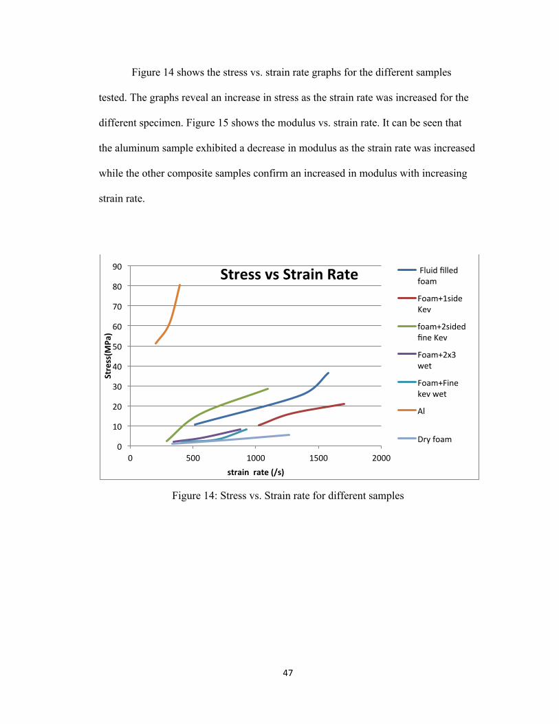
Figure 14 shows the stress vs. strain rate graphs for the different samples

tested. The graphs reveal an increase in stress as the strain rate was increased for the

different specimen. Figure 15 shows the modulus vs. strain rate. It can be seen that

the aluminum sample exhibited a decrease in modulus as the strain rate was increased

while the other composite samples confirm an increased in modulus with increasing

strain rate.

 

Figure 14: Stress vs. Strain rate for different samples

0  

10  

20  

30  

40  

50  

60  

70  

80  

90  

0   500   1000   1500   2000  

Stress(M

Pa)  

strain    rate  (/s)  

Stress  vs  Strain  Rate    Fluid  filled  foam  

Foam+1side  Kev  

foam+2sided  fine  Kev  

Foam+2x3  wet  

Foam+Fine  kev  wet  

Al  

Dry  foam  

48    

 

Figure 15: Modulus vs. Strain rate for the different sample tested

According to Zukas et al. (1982), this increase in stiffness is due to the

increase in the cross-sectional area of the specimen. The sample strains upon impact

and expands, increasing its surface area to the load. Because the aluminum sample is

made of a material with a higher modulus of elasticity, it will not experience as large

a change in cross-section as the polyurethane foam. Also, the material work-hardens

as deformation proceeds, making it stiffer as strain increases (Zukas et al., 1982).

This explains the increase in the modulus of the foam and composite specimens as the

strain rate or impact velocity increases between the ranges of 100 s-1 to 1500 s-1.

5.2. Results of Foam Samples from LANL  

The following Table 11 gives the properties of the SHPB apparatus at Los

Alamos National Laboratory. The testing was done on the SHPB with 9.525 mm

1  

5  

25  

125  

625  

3125  

0   500   1000   1500   2000  

Mod

ulus  (M

Pa)  

Strain  rate  (/s)  

Modulus  (MPa)  vs  Strain  Rate    Foam  

Foam+1side  Kev  

Foam  +  2  side  fine  Kev  

Foam+2x3  wet  

Foam+  fine  Kev  wet  

Al  

Foam  dry  

49    

diameter magnesium bars. The researchers at Los Alamos National Laboratory use

solid bars with very small diameter to achieve a higher strain rate.

Table 11: The properties of the SHPB material at LANL

The stress strain graph shown in Figure 16 was obtained after testing the polyurethane

foam at three different pressures at room temperature. The sample was 7.9375 mm in

diameter and 4.7325 mm thick. Due to the soft nature of the specimen, the transmitted

signal detected by the strain gauge on the solid output bar was unreliable to be used

for any analysis. It was then decided to increase the breech pressure for a higher

Breech Pressure(psi) 5.0

Striker Length(mm) 152.4

Incident Bar Young's Modulus(GPa) 42.957893

Incident Bar Poisson Ratio 0.310749

Incident Bar Rod Sound Speed(m/s) 4913.981418

Incident Bar Longitudinal Sound Speed(m/s) 5792

Incident Bar Shear Sound Speed(m/s) 3035

Incident Bar Density(kg/m^3) 1.779

Transmitted Bar Young's Modulus(GPa) 42.957893

Transmitted Bar Poisson Ratio 0.310749

Transmitted Bar Rod Sound Speed(m/s) 4913.981418

Transmitted Bar Longitudinal Sound Speed(m/s) 5792

Transmitted Bar Shear Sound Speed(m/s) 3035

Transmitted Bar Density(kg/m^3) 1.779

50    

impact velocity and better transmitted signal into the pressure bars. This did not

noticeably improve the results and the breech pressure could not be increased further

because higher impact velocity could yield the pressure bars. After analyzing these

results, it was decided to test the samples at lower temperature. The results at

different temperatures are discussed below. Figure 17 shows the average strain rate

vs. average strain for temperatures between 00C to -600C. It demonstrated the

constant strain rate required for SHPB testing (Gray, 2000). Figures 18 - 25 display

the results of the foam material tested at temperatures between 00C and -800C.

 

 

Figure 16: The stress-strain graph of polyurethane foam at room temperature

-­‐3.00E-­‐01  

-­‐2.00E-­‐01  

-­‐1.00E-­‐01  

0.00E+00  

1.00E-­‐01  

2.00E-­‐01  

3.00E-­‐01  

4.00E-­‐01  

5.00E-­‐01  

0.00E+00  2.00E-­‐02  4.00E-­‐02  6.00E-­‐02  8.00E-­‐02  1.00E-­‐01  1.20E-­‐01  1.40E-­‐01  1.60E-­‐01  1.80E-­‐01  

Stress  (M

Pa)  

Strain  

Stress  vs  Strain  8  psi  test  6  Psi  test  5  psi  test  

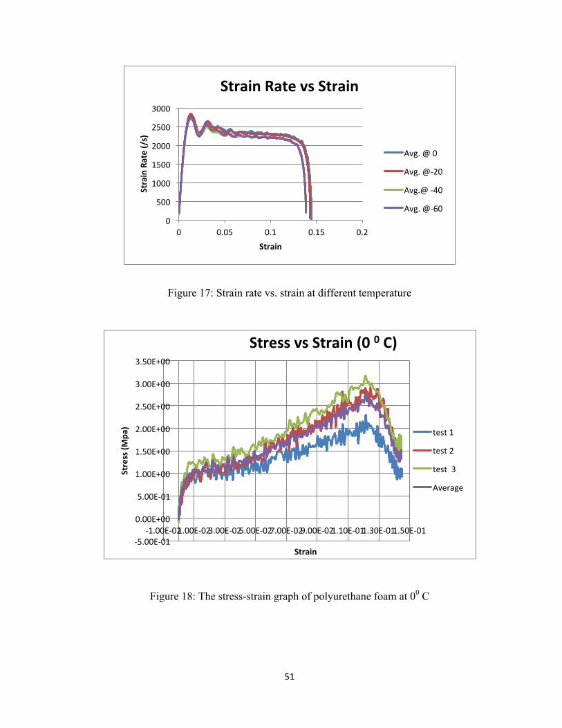
51    

 

Figure 17: Strain rate vs. strain at different temperature

 

Figure 18: The stress-strain graph of polyurethane foam at 00 C

0  

500  

1000  

1500  

2000  

2500  

3000  

0   0.05   0.1   0.15   0.2  

Strain  Rate  (/s)  

Strain  

Strain  Rate  vs  Strain  

Avg.  @  0  

Avg.  @-­‐20  

Avg.@  -­‐40  

Avg.  @-­‐60  

-­‐5.00E-­‐01  

0.00E+00  

5.00E-­‐01  

1.00E+00  

1.50E+00  

2.00E+00  

2.50E+00  

3.00E+00  

3.50E+00  

-­‐1.00E-­‐02  1.00E-­‐02  3.00E-­‐02  5.00E-­‐02  7.00E-­‐02  9.00E-­‐02  1.10E-­‐01  1.30E-­‐01  1.50E-­‐01  

Stress  (M

pa)  

Strain  

Stress  vs  Strain  (0  0  C)  

test  1  

test  2  

test    3  

Average  

52    

 

Figure 19: The stress-strain graph of polyurethane foam at -200 C

 

Figure 20: The stress-strain graph of polyurethane foam at -400 C

-­‐5.00E-­‐01  

0.00E+00  

5.00E-­‐01  

1.00E+00  

1.50E+00  

2.00E+00  

2.50E+00  

3.00E+00  

3.50E+00  

4.00E+00  

4.50E+00  

0.00E+00   5.00E-­‐02   1.00E-­‐01   1.50E-­‐01  

Stress  (M

Pa)  

Strain  

Stress  vs  Strain  (-­‐20  0  C)  

Test  1  

Test  2  

Test  3  

Average  

-­‐1.00E+00  

0.00E+00  

1.00E+00  

2.00E+00  

3.00E+00  

4.00E+00  

5.00E+00  

0.00E+00  2.00E-­‐02  4.00E-­‐02  6.00E-­‐02  8.00E-­‐02  1.00E-­‐01  1.20E-­‐01  1.40E-­‐01  1.60E-­‐01  

Stress  (M

Pa)  

Strain  

Stress  vs  Strain  (-­‐40  0  C)  

Test  1  

Test  2  

Test  3  

Average  

53    

 

Figure 21: The stress-strain graph of polyurethane foam at -600 C

 

Figure 22: The stress-strain graph of polyurethane foam at -800 C

-­‐1.00E+00  

0.00E+00  

1.00E+00  

2.00E+00  

3.00E+00  

4.00E+00  

5.00E+00  

6.00E+00  

0.00E+00  2.00E-­‐02  4.00E-­‐02  6.00E-­‐02  8.00E-­‐02  1.00E-­‐01  1.20E-­‐01  1.40E-­‐01  1.60E-­‐01  

Stress  (M

Pa)  

Strain  

Stress  vs  Strain  (-­‐600  C)  

Test  1  

Test  2  

Test  3  

Average  

0.00E+00  

5.00E-­‐01  

1.00E+00  

1.50E+00  

2.00E+00  

2.50E+00  

0.00E+00   5.00E-­‐02   1.00E-­‐01   1.50E-­‐01  

Stress  (M

Pa)  

Strain  

Stress  vs  Strain  (-­‐80  0  C  @  5.5  psi)  

54    

 

Figure 23: The stress-strain graph of polyurethane foam at -800 C

 

Figure 24: The stress-strain graph of polyurethane foam at -800 C

-­‐1.00E+00  

0.00E+00  

1.00E+00  

2.00E+00  

3.00E+00  

4.00E+00  

5.00E+00  

6.00E+00  

0.00E+00   4.00E-­‐02   8.00E-­‐02   1.20E-­‐01   1.60E-­‐01   2.00E-­‐01  

Stress  (M

Pa)  

Strain  

Stress  vs  Strain  (-­‐80  0  C  @  7psi)  

0.00E+00  

1.00E+00  

2.00E+00  

3.00E+00  

4.00E+00  

5.00E+00  

6.00E+00  

7.00E+00  

0.00E+00   5.00E-­‐02   1.00E-­‐01   1.50E-­‐01   2.00E-­‐01   2.50E-­‐01  

Stress  (M

Pa)  

Strain  

Stress  vs  Strain  (-­‐80  0  C@  11  psi)  

55    

 

Figure 25: Stress-strain graph of polyurethane foam at different temperatures

According to the Siviour et al. (2005) yield and flow stress for some polymers

increase with decreasing temperature; Figure 26 shows the stress vs. temperature for

the foam specimen and the increase in yield stress with decreasing temperature is

evident. Using the data obtained from the low temperature experiments Figures 27

and 28 were developed to deduce a relationship between modulus and strain rate.

Figure 25 yield Equation (17) with modulus as a function of temperature.

𝑦 =  −0.5839𝑥 + 16.906 (17)

Figure 26 yield Equation (18) with strain rate as a function of temperature

𝑦 =  −1.3167𝑥 + 1508 (18)

-­‐1  

0  

1  

2  

3  

4  

5  

6  

0   0.02   0.04   0.06   0.08   0.1   0.12   0.14   0.16  

Stress  (M

Pa)  

Strain  

Stress  vs  Strain  (average)  

0  C  

-­‐20  C  

-­‐40  C  

-­‐60  C  

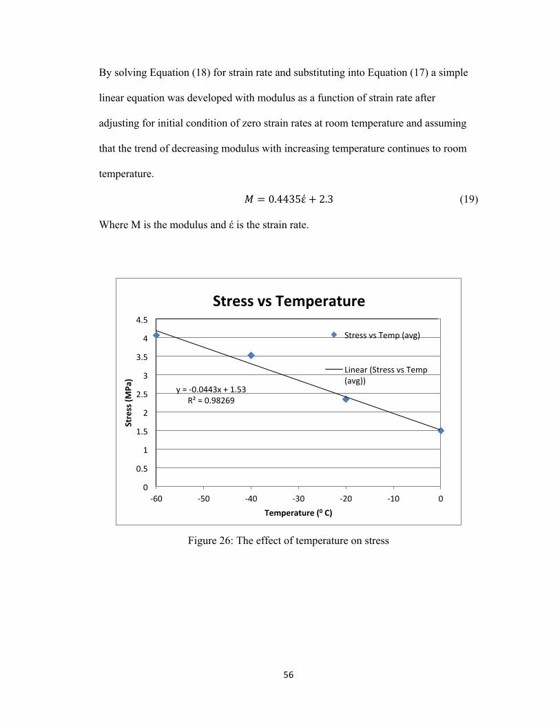
56    

By solving Equation (18) for strain rate and substituting into Equation (17) a simple

linear equation was developed with modulus as a function of strain rate after

adjusting for initial condition of zero strain rates at room temperature and assuming

that the trend of decreasing modulus with increasing temperature continues to room

temperature.

𝑀 = 0.4435έ+ 2.3 (19)

Where M is the modulus and έ is the strain rate.

 

Figure 26: The effect of temperature on stress

y  =  -­‐0.0443x  +  1.53  R²  =  0.98269  

0  

0.5  

1  

1.5  

2  

2.5  

3  

3.5  

4  

4.5  

-­‐60   -­‐50   -­‐40   -­‐30   -­‐20   -­‐10   0  

Stress  (M

Pa)  

Temperature  (0  C)  

Stress  vs  Temperature    

Stress  vs  Temp  (avg)  

Linear  (Stress  vs  Temp  (avg))  

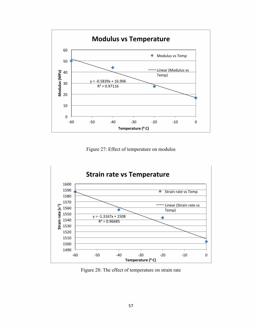
57    

 

Figure 27: Effect of temperature on modulus

 

 

Figure 28: The effect of temperature on strain rate

 

y  =  -­‐0.5839x  +  16.906  R²  =  0.97116  

0  

10  

20  

30  

40  

50  

60  

-­‐60   -­‐50   -­‐40   -­‐30   -­‐20   -­‐10   0  

Mod

ulus  (M

Pa)  

Temperature  (0  C)  

Modulus  vs  Temperature  

Modulus  vs  Temp  

Linear  (Modulus  vs  Temp)  

y  =  -­‐1.3167x  +  1508  R²  =  0.96685  

1490  1500  1510  1520  1530  1540  1550  1560  1570  1580  1590  1600  

-­‐60   -­‐50   -­‐40   -­‐30   -­‐20   -­‐10   0  

Strain  ra

te  (s

-­‐1)  

Temperature  (0  C)  

Strain  rate  vs  Temperature  

Strain  rate  vs  Temp  

Linear  (Strain  rate  vs  Temp)  

58    

As expected, the material stress increased as the temperature was lowered. In

fact, the stresses and the strain at yield increased with decreasing temperature. This is

consistent with other researchers that have investigated material properties as a

function of temperature (Siviour et al., 2005). Meyers (1994) also agreed that most

materials yield stress increases with strain rate and yield stress increase is more

marked at lower temperatures. Maximum stress of 6 MPa was achieved in the

specimen at an average strain rate of about 2000 s-1. At room temperature, the

maximum strain rate of approximately 2100 s-1 was attained for this material.

Utilizing solid pressure bars of 9.525 mm diameter and temperatures between

00C and -600C, the maximum strain rate of 2000 s-1 for the quick-recovery

polyurethane foam was achieved. Testing with hollow pressure bars at room

temperature yielded a maximum strain rate of 1400 s-1. The sandwiched composite

samples could not be tested on the 7.525 mm bars because it was not feasible to

prepare samples of 7.9375 mm diameter, the size needed for testing such bars. Also,

only dry samples were tested at Los Alamos National Laboratory because testing was

done between 0 and -800 C and therefore testing fluid filled samples was not possible.

Figure 29 shows the dynamic modulus as function of strain rate of the

different samples tested compared with the theoretical data obtained from Equation

(19) developed with data from the modulus vs. temperature data and from the strain

rate vs. temperature graphs. A simple relationship was developed to determine the

modulus of this composite material as function of strain rate, as shown in Figure 29.

59    

 

Figure 29: Comparison of the theoretical and experimental data

 

Additional tests were carried out on the foam samples on the SHPB at NMT to

gather data to verify Equation (19) since Equation (19) was developed by testing the

foam at temperatures of 0 0C to -60 0C. The foam sample was tested at breech

pressures of 5, 10, and 15 psi corresponding to average strain rates of 731, 887, and

1260 s-1 respectively. The foam sample measured 25.4 mm in diameter and 4.7625

mm in length. Figure 30 below compares the theoretical data from Equation (19) and

the actual test data of the foam specimen.

y  =  0.4435x  +  2.3  

1  

5  

25  

125  

625  

3125  

0   500   1000   1500   2000   2500  

Mod

ulus  (M

Pa)  

Strain  rate  (/s)  

Modulus  (MPa)  vs  Strain  Rate    Foam  

Foam+1side  Kev  

Foam  +  2  side  fine  Kev  

Foam+2x3  wet  

Foam+  fine  Kev  wet  

Al  

TheoreZcal  Modulus  vs  strain  rate  

Foam  dry  

Linear  (TheoreZcal  Modulus  vs  strain  rate)  

60    

 

Figure 30: Comparison of the theoretical and experimental data

The experimental and theoretical data are in close agreement. This implies

that tests done at low temperatures provided the valuable data that was used to

develop Equation (19). The major differences between the two sets of data are the

values of zero strain rates. According to Equation (19), zero strain rates yielded a

modulus of 2.3 MPa, while the trend line for actual test data predicted a modulus of

72.258 MPa. The lower modulus at zero strain rates from Equation (19) resulted from

the assumption that the trend of decreasing modulus with increasing temperature as

shown in Figure 27 continued to room temperature. Also, the theoretical data reveals

that the rate of increase in modulus with strain rate is 0.4435 while the experimental

data shows the modulus increase at a rate 0.3203 with strain rate, as shown in

Equation (20).

𝑀 = 0.3203έ+ 72.258 (20)

y  =  0.3203x  +  72.258  R²  =  0.98427  

y  =  0.4435x  +  2.3  R²  =  1  

0  

100  

200  

300  

400  

500  

600  

0   500   1000  

Mod

ulus  (M

Pa)  

Strain  rate  (/s)  

Modulus  (MPa)  vs.  Strain  Rate  Foam  

TheoreZcal  data  

Linear  (Foam)  

Linear  (TheoreZcal  data)  

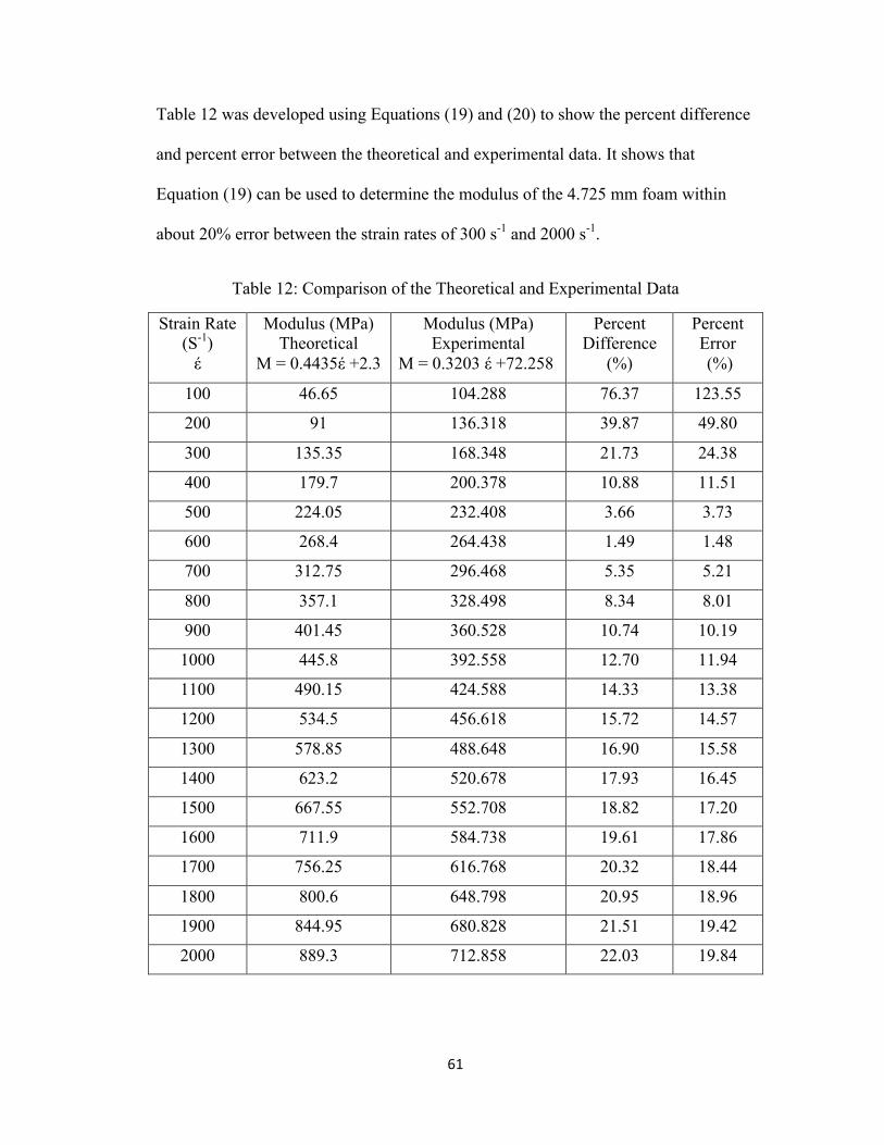
61    

Table 12 was developed using Equations (19) and (20) to show the percent difference

and percent error between the theoretical and experimental data. It shows that

Equation (19) can be used to determine the modulus of the 4.725 mm foam within

about 20% error between the strain rates of 300 s-1 and 2000 s-1.

Table 12: Comparison of the Theoretical and Experimental Data Strain Rate

(S-1) έ

Modulus (MPa) Theoretical

M = 0.4435έ +2.3

Modulus (MPa) Experimental

M = 0.3203 έ +72.258

Percent Difference

(%)

Percent Error (%)

100 46.65 104.288 76.37 123.55

200 91 136.318 39.87 49.80

300 135.35 168.348 21.73 24.38

400 179.7 200.378 10.88 11.51

500 224.05 232.408 3.66 3.73

600 268.4 264.438 1.49 1.48

700 312.75 296.468 5.35 5.21

800 357.1 328.498 8.34 8.01

900 401.45 360.528 10.74 10.19

1000 445.8 392.558 12.70 11.94

1100 490.15 424.588 14.33 13.38

1200 534.5 456.618 15.72 14.57

1300 578.85 488.648 16.90 15.58

1400 623.2 520.678 17.93 16.45

1500 667.55 552.708 18.82 17.20

1600 711.9 584.738 19.61 17.86

1700 756.25 616.768 20.32 18.44

1800 800.6 648.798 20.95 18.96

1900 844.95 680.828 21.51 19.42

2000 889.3 712.858 22.03 19.84

62    

The data from Table 12 was then used to produce Figure 31 which shows the

percent error against strain rate. It is evident from this figure that strain rates between

100 s-1 and 300 s-1 have a high percent error. As mention earlier the constants in

Equations (19) and (20) are quite different and may have influenced this error.

However, these equations are valid for strain rates between 300 s-1 and 2000 s-1 and

will serve as a starting point for developing the constitutive equation needed for

characterizing this polyurethane foam composite under impact loading.

 

Figure 31: Percent Error vs. Strain Rate

0.00  

20.00  

40.00  

60.00  

80.00  

100.00  

120.00  

140.00  

0   500   1000   1500   2000   2500  

Percen

t  Error  

Strain  Rate  (/s)  

Percent  Error  vs.  Strain  Rate  

63    

CHAPTER 6 CONCLUSIONS  

The necessary modifications were made to the SHPB apparatus at New

Mexico Tech’s laboratory and experiments were carefully conducted to determine the

composite material’s response to high strain rate loading. By increasing the impact

velocities, the strain rates of the specimen were increased and the material exhibited

an increase in dynamic modulus. The same trend was observed when the wet samples

were tested. The strain rates obtained were between 100 s-1 and 1500 s-1 for 10.7 to

19.8 m/s impact velocities. Higher impact velocities could not be achieved on the

current SHPB setup because it will produce yielding in the pressure bars and

ultimately invalid data. According to the literature, smaller bars should be used for

higher strain rates.

At low temperatures the yield stress increases with decreasing temperature.

The low temperature tests resulted in the development of a simple relation that

predicts modulus as a function of strain rate. This new composite developed by

researchers at New Mexico Tech is a multifunctional material. Testing revealed it’s

excellence in acoustic dampening (Ghosh et al., 2007), induced convection during

heating (Ghosh et al., 2010), and in this study, increased stiffness with increasing

strain rates. The SHPB can be used to produce consistent data needed to formulate

models of the constitutive properties of this new composite material.

   

64    

CHAPTER 7 FUTURE WORK  

Results of this research shown that the composite experienced an increased in

stiffness with increasing strain rates between the range of 100 s-1 and 1500 s-1. This is

encouraging results and additional testing methods must be explored for a better

understanding of this composite’s behavior so that the range of applications for this

material can be expanded. Also, additional tests will ultimately result in the

development of constitutive equations that will predict this material behavior at high

strain rates.

1. Further modification of the Split Hopkinson pressure bar can be explored with

the aim of obtaining higher strain rates by employing smaller pressure bars

and an output bar with a thinner wall. This modification will be intense since

most parts of the apparatus will have to be replaced.

2. Other high strain rate testing methods should be explored to determine this

material behavior at higher strain rate (See Meyers pg. 299).

3. Testing this material in an explosive environment can also provide valuable

insight to its behavior at higher strain rates, therefore it should be pursued.

4. Preparing multi-layers samples, i.e. samples with different skin layers (e.g.

Kevlar+Foam+carbon fiber) for testing under different loading conditions.

5. Taylor Impact test should be done for more in-depth investigation of the

material’s behavior.

   

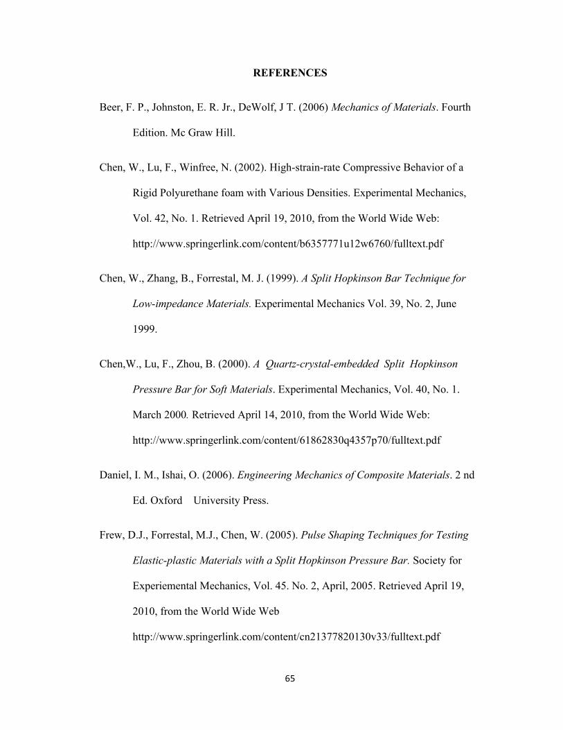
65    

REFERENCES  

Beer, F. P., Johnston, E. R. Jr., DeWolf, J T. (2006) Mechanics of Materials. Fourth

Edition. Mc Graw Hill.

Chen, W., Lu, F., Winfree, N. (2002). High-strain-rate Compressive Behavior of a

Rigid Polyurethane foam with Various Densities. Experimental Mechanics,

Vol. 42, No. 1. Retrieved April 19, 2010, from the World Wide Web:

http://www.springerlink.com/content/b6357771u12w6760/fulltext.pdf

Chen, W., Zhang, B., Forrestal, M. J. (1999). A Split Hopkinson Bar Technique for

Low-impedance Materials. Experimental Mechanics Vol. 39, No. 2, June

1999.

Chen,W., Lu, F., Zhou, B. (2000). A Quartz-crystal-embedded Split Hopkinson

Pressure Bar for Soft Materials. Experimental Mechanics, Vol. 40, No. 1.

March 2000. Retrieved April 14, 2010, from the World Wide Web:

http://www.springerlink.com/content/61862830q4357p70/fulltext.pdf

Daniel, I. M., Ishai, O. (2006). Engineering Mechanics of Composite Materials. 2 nd

Ed. Oxford University Press.

Frew, D.J., Forrestal, M.J., Chen, W. (2005). Pulse Shaping Techniques for Testing

Elastic-plastic Materials with a Split Hopkinson Pressure Bar. Society for

Experiemental Mechanics, Vol. 45. No. 2, April, 2005. Retrieved April 19,

2010, from the World Wide Web

http://www.springerlink.com/content/cn21377820130v33/fulltext.pdf

66    

Ghosh, A. K., Morton, B., Birbahadur, N., Chavez, P., Sewal, E., Luders, I., Chavez,

D. (2010). A Novel Material for an Adaptive and Stealth Naval Plotform (Rep.

No. N00014-09-M-0005).

Ghosh, A. K., Williams, A. D., Zucker, J. M. Mathews, J. L., Spinhirne, N. (2007).

An Experimental Investigation into Acoustic Characteristics of Fluid-filled

Porous Structures – A Simplified Model of the Human Skull Cancellous

Structure. Experimental Mechanics.

Graff, K. R. (1991). Wave Motion in Elastic Solids. Dover Publication.

Gray, G. T, (2000). Classical Split-Hopkinson Pressure Bar Testing. Mechanical

Testing and evaluation, metals handbook. American Society for Metals.

Gray, G. T., Blumenthal, W. R. (2000). Split Hopkinson Pressure Bar Testing of Soft

Materials. American Society for Metals, Vol. 8, 2000.

Harding, J. (1979). Mechanical Properties at High Rates of Strain. Department of

Engineering Science, University of Oxford.

Humphrey, J. D. (2002). Continuum biomechanics of soft biological tissues.

Retrieved December 04, 2009, from the World Wide Web:

http://www.see.ed.ac.uk/~vkoutsos/Literature%20for%20Challenging%20Eng

ineering%20Proposal/Continuum%20biomechanics%20of%20Soft%20Biolog

ical%20Tissues.pdf

Johnson, T.P.M., Sarva, S.S., Socrate, S. (2009). Comparison of Low Impedance

Split-Hopkinson Pressure Bar Techniques in the Characterization of

67    

Polyurea. Experimental Mechanics, 2009. Retrieved April 19, 2010, from the

World Wide Web:

http://www.springerlink.com/content/h561603387n02445/fulltext.pdf

Kaisers, M. A. (1998). Advancements in the Split Hopkinson Bar Test. MS thesis, VPI

1998. Retrieved December 07, 2009, from the World Wide Web:

http://scholar.lib.vt.edu/theses/available/etd-41998-

18465/unrestricted/ETD.pdf

Kolsky, H. (1949). An Investigation of the Mechanical Properties of Materials at very

High Rates of Loading. Retrieved October 11, 2010, from the World Wide

Web: http://iopscience.iop.org/0370-1301/62/11/302/pdf/0370-

1301_62_11_302.pdf

Kolsky, H. (1963). Stress Waves in Solids. Dover Publications Inc , pg. 87.

Kukureka, S. N., Hutchings, I. M. (1984). Yielding of Engineering Polymers at Strain

Rate of up to 500 s-1. Int. J. Mech. Sci.,Vol. 26, 1984, p 617-623.

Lindholm, U.S., Yeakley, L. M. (1968). High Strain Rate Testing: Tension and

Compression. Experimental Mechanics, January 1968. Retrieved September

25, 2010, for the World Wide Web:

http://www.springerlink.com/content/1w656064t3113116/fulltext.pdf

Malvern, L. E. (1969). Introduction to the Mechanics of a Continuous Medium.

Prentice-Hall.

68    

Mathews, J. (2008). Shock and Vibration Characteristics of a Bio-Inspired Structure

under Blast Loading MS Thesis, New Mexico Institute of Mining and

Technology.

Meyers, M. A. (1994). Dynamic behavior of Materials. Wiley.

Ninan, L., Tsai, J., Sun, C. T., (2001). Use of Split Hopkinson Pressure Bar for off-

axis composites. International Journal of Impact Engineering 25, 2001.

Retrieved December 12, 2009, from the World Wide Web:

http://www.sciencedirect.com/science?_ob=MImg&_imagekey=B6V3K-

423YKFN-5-

4R&_cdi=5733&_user=1818435&_orig=search&_coverDate=03%2F31%2F2

001&_sk=999749996&view=c&wchp=dGLbVlz-

zSkzV&md5=922e617ee36230d5a952f012a7b92d53&ie=/sdarticle.pdf

Owens, A.T., Tippur, H.V. (2009). A Tensile Split Hopkinson Bar for Testing

Particulate Polymer Composites Under Elevated Rates of Loading.

Experimental Mechanics. Retrieved April 19, 2010, form the World Wide

Web: http://www.springerlink.com/content/k17q0061711326l6/fulltext.pdf

Rogers Corporation, 2010.

http://www.rogerscorporation.com/hpf/CT/PoronI/industrial_tech_info.htm

Sharma, A., Shukla, A., Prosser, R. A. (2002). Mechanical characterization of soft

materials using high speed photography and split Hopkinson pressure bar

technique. Journal of Materials Science. Retrieved April 19, 2010, from the

69    

World Wide Web:

http://www.springerlink.com/content/5uj5ybyja924g379/fulltext.pdf

Siviour, C.R., Walley, S.M., Proud, W.G., Field, J.E. (2005). The high strain rate

compressive behavior of polycarbonate and polyvinylidene difluoride .

November 2005. Retrieved February 10, 2011 form the World Wide Web:

http://www.sciencedirect.com/science?_ob=MImg&_imagekey=B6TXW-

4HJ47YW-8-

1X&_cdi=5601&_user=1818435&_pii=S0032386105015806&_origin=searc

h&_coverDate=12%2F12%2F2005&_sk=999539973&view=c&wchp=dGLb

Vlb-zSkzS&md5=54967e8ff56b1bc23448c21696428fe2&ie=/sdarticle.pdf

Slaughter, W. S. (2002). The Linearized Theory of Elasticity. Birkhauser.

Song, B., Chen, W. (2004). Dynamic Stress Equilibration in Split Hopkinson

Pressure Bar Tests on Soft Materials. Experimental Mechanics Vol. 44, No. 3,

June 2004. Retrieved April 19, 2010, from the World Wide Web:

http://www.springerlink.com/content/guh311h3j692p610/fulltext.pdf

Song, B., Chen, W. (2005). Split Hopkinson pressure bar technique for

characterizing soft materials. Latin America Journal of Solids and Structures

2, 2005. Retrieved April 14, 2010, from the World Wide Web:

http://www.lajss.org/index.php/LAJSS/article/viewFile/73/67

Walley, S. M., Field, J. E., Safford, N. A. (1991). A Comparison of the High Strain

Rate Behavior in Compression of Polymers at 300K and 100K, J. Phys.

(France) IV Colloq. C3 (DYMAT 91), Vol. 1, 1991, P 185-190.

70    

Zukas, J. A., Nicholas, T., Swift, H. F., Greszczuk, L. B., Curran, D. R. (1982).

IMPACT DYNAMICS. John Wiley & Sons, pg. 287-288.