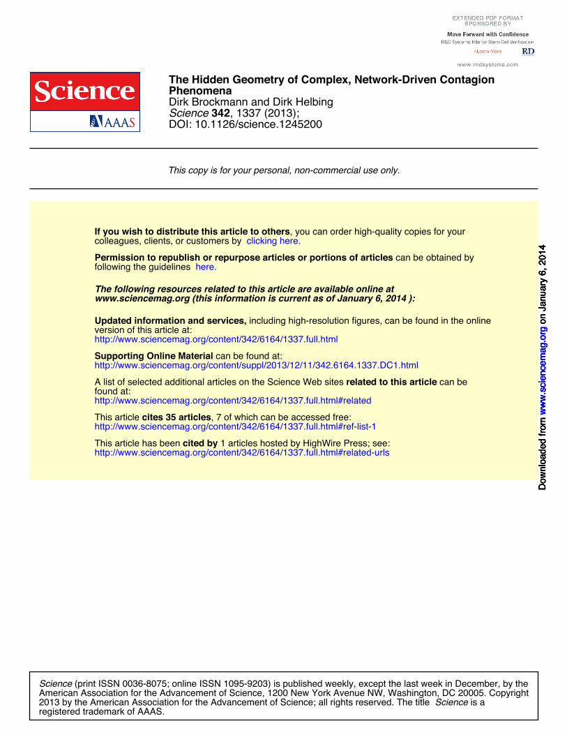
DOI: 10.1126/science.1245200, 1337 (2013);342 Science

Dirk Brockmann and Dirk HelbingPhenomenaThe Hidden Geometry of Complex, Network-Driven Contagion

This copy is for your personal, non-commercial use only.

clicking here.colleagues, clients, or customers by , you can order high-quality copies for yourIf you wish to distribute this article to others

here.following the guidelines

can be obtained byPermission to republish or repurpose articles or portions of articles

): January 6, 2014 www.sciencemag.org (this information is current as of

The following resources related to this article are available online at

http://www.sciencemag.org/content/342/6164/1337.full.htmlversion of this article at:

including high-resolution figures, can be found in the onlineUpdated information and services,

http://www.sciencemag.org/content/suppl/2013/12/11/342.6164.1337.DC1.html can be found at: Supporting Online Material

http://www.sciencemag.org/content/342/6164/1337.full.html#relatedfound at:

can berelated to this article A list of selected additional articles on the Science Web sites

http://www.sciencemag.org/content/342/6164/1337.full.html#ref-list-1, 7 of which can be accessed free:cites 35 articlesThis article

http://www.sciencemag.org/content/342/6164/1337.full.html#related-urls1 articles hosted by HighWire Press; see:cited by This article has been

registered trademark of AAAS. is aScience2013 by the American Association for the Advancement of Science; all rights reserved. The title

CopyrightAmerican Association for the Advancement of Science, 1200 New York Avenue NW, Washington, DC 20005. (print ISSN 0036-8075; online ISSN 1095-9203) is published weekly, except the last week in December, by theScience

on

Janu

ary

6, 2

014

ww

w.s

cien

cem

ag.o

rgD

ownl

oade

d fro

m

on

Janu

ary

6, 2

014

ww

w.s

cien

cem

ag.o

rgD

ownl

oade

d fro

m

on

Janu

ary

6, 2

014

ww

w.s

cien

cem

ag.o

rgD

ownl

oade

d fro

m

on

Janu

ary

6, 2

014

ww

w.s

cien

cem

ag.o

rgD

ownl

oade

d fro

m

on

Janu

ary

6, 2

014

ww

w.s

cien

cem

ag.o

rgD

ownl

oade

d fro

m

on

Janu

ary

6, 2

014

ww

w.s

cien

cem

ag.o

rgD

ownl

oade

d fro

m

on

Janu

ary

6, 2

014

ww

w.s

cien

cem

ag.o

rgD

ownl

oade

d fro

m

The Hidden Geometry of Complex,Network-Driven Contagion PhenomenaDirk Brockmann1,2,3* and Dirk Helbing4,5

The global spread of epidemics, rumors, opinions, and innovations are complex, network-drivendynamic processes. The combined multiscale nature and intrinsic heterogeneity of the underlyingnetworks make it difficult to develop an intuitive understanding of these processes, to distinguish relevantfrom peripheral factors, to predict their time course, and to locate their origin. However, we show thatcomplex spatiotemporal patterns can be reduced to surprisingly simple, homogeneous wave propagationpatterns, if conventional geographic distance is replaced by a probabilistically motivated effectivedistance. In the context of global, air-traffic–mediated epidemics, we show that effective distance reliablypredicts disease arrival times. Even if epidemiological parameters are unknown, themethod can still deliverrelative arrival times. The approach can also identify the spatial origin of spreading processes andsuccessfully be applied to data of the worldwide 2009 H1N1 influenza pandemic and 2003 SARS epidemic.

The geographic spread of emergent infec-tious diseases affects the lives of tens ofthousands or evenmillions of people (1, 2).

Recent examples of emergent diseases are theSARS epidemic of 2003, the 2009 H1N1 influenzapandemic, and most recently a new strain (H7N9)of avian influenza virus (3, 4). Progressingworld-wide urbanization, combined with growing con-nectivity amongmetropolitan centers, has increasedthe risk that highly virulent emergent pathogenswill spread (5–8). The complexity of global hu-man mobility, particularly air traffic (Fig. 1A),makes it increasingly difficult to develop effec-tive containment andmitigation strategies on thetime scale imposed by the speed at which mod-ern diseases can spread (9–11). Because timely,accurate, and focused action can potentially savethe lives of many people and reduce the socio-economic impact of infectious diseases (12, 13),understanding global disease dynamics has be-come a major 21st-century challenge. Unravelingthe core mechanisms that underlie these phenome-na and being able to distinguish key factors fromperipheral ones are required to develop quantita-tive, efficient, and predictive models that publichealth authorities can employ to assess situationsquickly, make informed decisions, and optimizevaccination and drug delivery plans. After the in-itial outbreak of an epidemic, the key questions areas follows: (i)Where did the novel pathogen emerge?(ii)Where are new cases to be expected? (iii)Whenis an epidemic going to arrive at distant locations?(iv) How many cases are to be expected?

Historically, for cases like the spread of theBlack Death in Europe, reaction-diffusion mod-

els have been quite useful in addressing thesequestions (14, 15). Despite their high level ofabstraction, thesemodels provide a solid intuitionand understanding of spreading processes. Theirmathematical simplicity permits the assessmentof key properties, e.g., spreading speed, arrivaltimes, and how pattern geometry depends on sys-tem parameters (16). However, because of long-distance travel, simple reaction-diffusion modelsare inadequate for the description of today’s com-plex, spatially incoherent spreading patterns thatgenerically bear no metric regularity, that dependsensitively on model parameters and initial con-ditions (17–20) (Fig. 1, B to E, and fig. S2).

Consequently, scientists have been developingpowerful, large-scale computational models andsophisticated, parameter-rich epidemic simulatorsthat tackle the above key questions in detailedways. These consider demographics, mobility, andepidemiological data, as well as disease-specificmechanisms, all of which are believed to play arole (21–23). Models range from high-level sto-chastic metapopulationmodels (5, 20, 24) to agent-based computer simulations that account for thebehavior and interactions of millions of individualsin large populations (25). These approaches havebecome remarkably successful in reproducing ob-served patterns and predicting the temporal evo-lution of ongoing epidemics (26). Many suchmodels reproduce similar dynamic features despitemajor differences in their underlying assumptionsand data (27). The abundance of different, oftenmutually incompatible, models suggests that westill lack a fundamental understanding of the keyfactors that determine the observed spatiotemporaldynamics. It is unclear how the multitude of factorsshape the dynamics and how much detail is re-quired to achieve a certain level of predictive fidel-ity. Moreover, detailed computational models thatincorporate all potentially relevant factors ab initiodo not inform which factors are actually relevantand which ones are not (28). They are also hard tocalibrate and of limited use when the knowledgeof epidemiological parameters is uncertain.

Here, we propose an intuitive and efficientapproach that remedies the situation by connect-ing the conceptual power of simple reaction-diffusion systems with the predictive power ofhigh-level, computational models. Our approachis based on the idea of replacing conventionalgeographic distance by a measure of effectivedistance derived from the underlying mobilitynetwork. Based on this novel notion of distance,patterns that exhibit complex spatiotemporal struc-ture in the conventional geographic perspectiveturn into regular, wavelike solutions reminiscentof simple reaction-diffusion systems. This permitsthe definition of effective epidemic wavefronts,propagation speeds, and the reliable estimation ofepidemic arrival times, based on the knowledgeof the underlying mobility network. The method,however, goes beyond remapping data. It pro-vides two key insights. First, epidemiological pa-rameters enter the spreading dynamics separatelyfrom the transport parameters, and second, thedynamics is dominated by only a small percent-age of transport connections. Furthermore, ourapproach can quickly identify the geographicorigin of emergent diseases, using temporal snap-shots of the spatial disease distribution. Thisdetection of the origin of complex, multiscale dy-namical spreading patterns is important for threereasons: (i) to determine what has caused the dis-ease, (ii) to develop timely mitigation strategies,and (iii) to predict its further spread (the arrival timesin remote locations and the expected prevalence).

Modeling Network-Driven Contagion PhenomenaFor illustration, we consider a complex networkof coupled populations (ametapopulation) inwhichthe local disease time course is described by a con-ventional susceptible-infected-recovered (SIR) dy-namics (1):

∂tSn ¼ −aInSn=Nn,

∂tIn ¼ aInSn=Nn − bIn n ¼ 1,…,M (1)

where Nn is the population size of populationn, M is the number of populations, and Sn, In,Rn ¼ Nn − Sn − In are absolute numbers of sus-ceptible, infected, and recovered individuals, re-spectively. Parameter b is the mean recovery rateof individuals (for influenza-like diseases b–1 =3 to 5 days), and R0 = a/b is the basic repro-duction ratio (for whichwe assume typical valuesin the range 1.4 to 2.9). (The focus on SIR kineticsis not essential, as the following results are alsovalid for other types of local dynamics.) Each lo-cal population represents a node n in the globalmobility network (GMN), depicted in Fig. 1A. Inaddition to the local dynamics, individuals travelbetween nodes according to the rate equation

∂tUn ¼ ∑m≠n

wnmUm − wmnUn ð2Þ

where Un is a placeholder for the classes Sn, In,and Rn. The quantities wnm = Fnm/Nm representthe per-capita traffic flux from location m to n.

RESEARCHARTICLE

1Robert-Koch-Institute, Seestraße 10, 13353 Berlin, Germany.2Institute for Theoretical Biology, Humboldt-University Berlin,Invalidenstraße 42, 10115 Berlin, Germany. 3Department ofEngineering Sciences and Applied Mathematics and NorthwesternInstitute on Complex Systems, Northwestern University, Evanston,IL 60208, USA. 4ETH Zurich, Swiss Federal Institute of Technology,CLU E1, Clausiusstraße 50, 8092 Zurich, Switzerland. 5Risk Cen-ter, ETH Zurich, Scheuchzerstraße 7, 8092 Zurich, Switzerland.

*Corresponding author. E-mail: dirk.brockmann@hu-berlin.de

www.sciencemag.org SCIENCE VOL 342 13 DECEMBER 2013 1337

Weighted links Fnm quantify direct air traffic(passengers per day) from node m to node n.The GMN is constructed from the worldwide airtraffic between 4069 airports with 25,453 directconnections. Details on the data and network con-struction are provided in the supplementary mate-rials (e.g., fig. S1 and table S1) (5, 13, 20, 29). Thetotal network traffic is approximately F ¼ 8:91$106 passengers per day. Assuming that the totaltraffic in and out of a node is proportional to itspopulation size, Eqs. 1 and 2 can be rewritten as

∂t jn ¼ asn jnsð jn=eÞ − b jn þ g ∑m≠n

Pmnð jm − jnÞ

∂tsn ¼ −asn jnsð jn=eÞ þ g ∑m≠n

Pmnðsm − snÞ

with sn = Sn/Nn, jn = In/Nn, and rn = 1 – sn – jn. Adetailed derivation is provided in the supplemen-tary text. The mobility parameter g is the averagemobility rate, i.e.,g ¼ F=W, whereW ¼ ∑nNn isthe total population in the system. This yields nu-merical values in the range g =0.0013–0.0178day–1.The matrix P with 0 ≤ Pmn ≤ 1 quantifies thefraction of the passenger flux with destinationm

emanating from node n, i.e., Pmn = Fmn/Fn,

where Fn ¼ ∑mFmn. The additional sigmoid func-

tion sðxÞ ¼ xh=ð1þ xhÞwithgainparameterh >>0accounts for the local invasion threshold e andfluctuation effects for jn < e (30–32). Typicalparameter choices for e and h areh ¼ 4,8,∞ and−log10 e ¼ 4,…,6. Our results are robust with re-spect to changes in these parameters (e.g., figs. S5and S13).

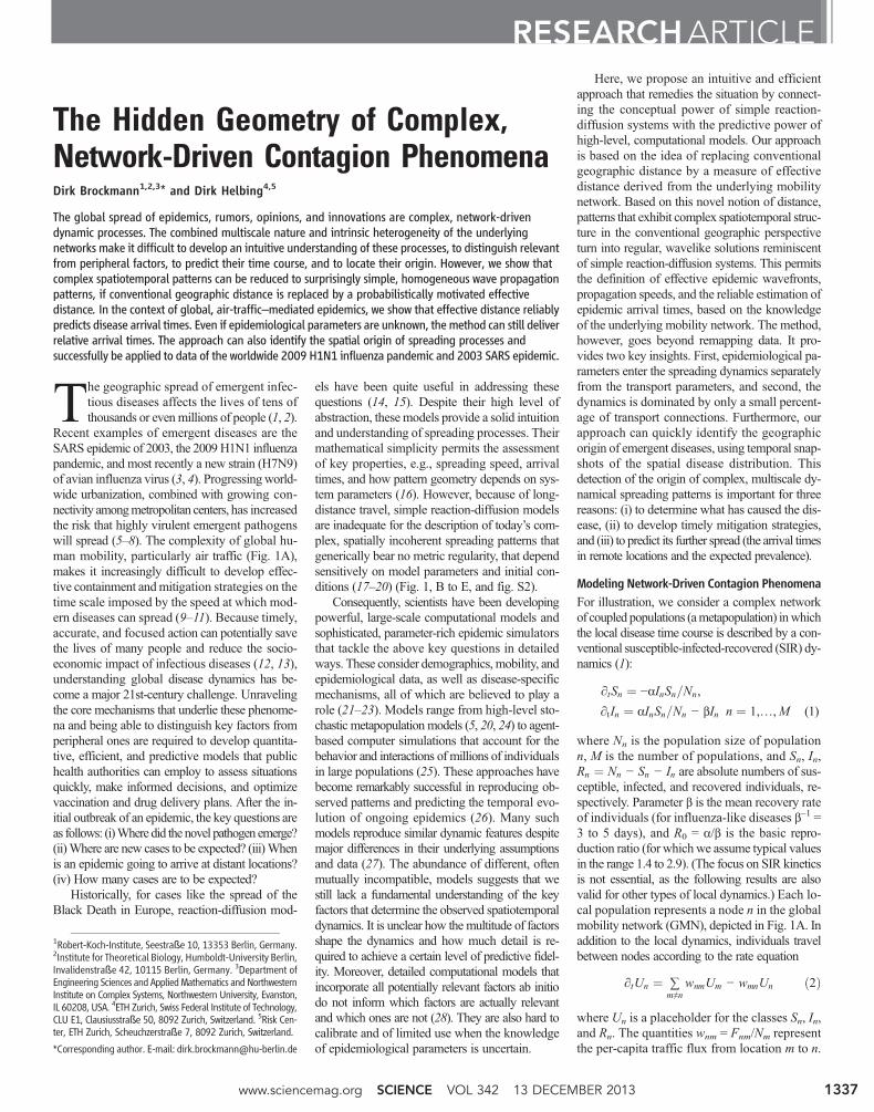
Figure 1B shows a temporal snapshot of thedynamical system defined by Eq. 3 for a hy-pothetical pandemic with initial outbreak loca-tion (OL) in HongKong (HKG) (see also Fig. 2Band fig. S2 for temporal sequences of the dy-namical system for various other OLs). General-ly, the metapopulation model above and relatedmodels used in the past generate solutions thatare characterized by similar qualitative features.First, only during the early stage of the processdoes the prevalence jn(t) (i.e., the fraction ofinfected individuals) correlate significantly withgeographic distance from the OL. Second, at in-

termediate and later stages, themultiscale structureof the GMN induces a spatial decoherence ofthe spreading pattern. Third, despite the globalconnectivity, the spatiotemporal patterns do notconverge to the same pattern, i.e., spatiotemporaldifferences are not a transient effect (figs. S3 toS6 andmovies S1 to S3). This type of complexitysharply contrasts the generic behavior of ordinaryreaction-diffusion systems, which typically ex-hibit spatially coherent wavefronts.

Most Probable Paths and Effective DistanceThe key idea we pursue here is that, despite thestructural complexity of the underlying network,the redundancy of connections, and the multiplic-ity of paths a contagion phenomenon can take, thedynamic process is dominated by a set of mostprobable trajectories that can be derived from theconnectivity matrix P. This hypothesis is analogousto the dominance of the smallest resistor in a strong-ly heterogeneous electrical network with parallelconducting lines.Given the flux-fraction0≤Pmn≤1,i.e., the fraction of travelers that leave node n and

A B

0 5 10 15 2020

40

60

80

100

120

140

160

180

200

220C

Dg [103 km]

T a [day

s]

Simulation (OL: HKG)

0 5 10 15 200

50

100

150D

Afghanistan

Argentina

Barbados

China

GermanySpain

France

UK

India

Italy

Japan

Latvia

Mexico

Norway

Slovenia

USA

Dg [103 km]

T a [day

s]

H1N1 (2009)

0 5 10 15 200

20

40

60

80

100

120

140

160

180

200E

USA

UK

Germany

FranceSpainItaly

China

Hong KongSingapore

Canada

Thailand

Korea

Switzerland

Ireland

Australia

India

Dg [103 km]

T a [day

s]SARS (2003)

Fig. 1. Complexity in global, network-driven contagion phenomena. (A)The global mobility network (GMN). Gray lines represent passenger flows alongdirect connections between 4069 airports worldwide. Geographic regions aredistinguished by color [classified according to network modularity maximization(39)]. (B) Temporal snapshot of a simulated global pandemic with initial outbreaklocation (OL) in Hong Kong (HKG). The simulation is based on themetapopulationmodel defined by Eq. 3 with parameters R0 = 1.5, b = 0.285 day–1, g = 2.8 ×10–3 day–1, e = 10–6. Red symbols depict locations with epidemic arrival timesin the time window 105 days≤ Ta≤ 110 days. Because of themultiscale structureof the underlying network, the spatial distribution of disease prevalence (i.e.,the fraction of infected individuals) lacks geometric coherence. No clear wave-front is visible, and based on this dynamic state, the OL cannot be easily deduced.(C) For the same simulation as in (B), the panel depicts arrival times Ta as afunction of geographic distance Dg from the OL [nodes are colored according togeographic region as in (A)] for each of the 4069 nodes in the network. On a

global scale, Ta weakly correlates with geographic distance Dg (R2 = 0.34). Alinear fit yields an average global spreading speed of vg = 331 km/day (see alsofig. S7). Using Dg and vg to estimate arrival times for specific locations, however,does not work well owing to the strong variability of the arrival times for a givengeographic distance. The red horizontal bar corresponds to the arrival timewindow shown in (B). (D) Arrival times versus geographic distance from thesource (Mexico) for the 2009 H1N1 pandemic. Symbols represent 140 affectedcountries, and symbol size quantifies total traffic per country. Arrival times aredefined as the date of the first confirmed case in a given country after the initialoutbreak on 17 March 2009. As in the simulated scenario, arrival time andgeographic distance are only weakly correlated (R2 = 0.0394). (E) In analogy to(D), the panel depicts the arrival times versus geographic distance from thesource (China) of the 2003 SARS epidemic for 29 affected countries worldwide.Arrival times are taken from WHO published data (2). As in (C) and (D), arrivaltime correlates weakly with geographic distance.

(3)

13 DECEMBER 2013 VOL 342 SCIENCE www.sciencemag.org1338

RESEARCH ARTICLE

arrive at node m, we define the effective distancednm from a node n to a connected node m as

dmn ¼ ð1 − logPmnÞ ≥ 1 ð4Þ

This concept of effective distance reflects theidea that a small fraction of traffic n→m is effec-tively equivalent to a large distance, and vice versa.As explained in more detail in the supplemen-tary text, the logarithm is a consequence of therequirement that effective lengths are additive,whereas probabilities along multistep paths aremultiplicative. Eq. 4 defines a quasi-distance,whichis generally asymmetric, i.e., dmn ≠ dnm. The lackof symmetry is analogous to a road network of one-way streets, where the shortest distance fromA toBmay differ from the one from B to A. This asym-metry captures the effect that a randomly seededdisease in a peripheral node of the network has ahigher probability of being transmitted to a well-connected hub than vice versa (figs. S8 to S10).More properties of effective distance as definedby Eq. 4 are discussed in the supplementary text.On the basis of effective distance, we can definethe directed length lðGÞ of an ordered path

G ¼ fn1,…,nLg as the sum of effective lengthsalong the legs of the path. Moreover, we definethe effective distance Dmn from an arbitrary ref-erence node n to another node m in the networkby the length of the shortest path from n to m:

Dmn ¼ minG

lðGÞ ð5Þ

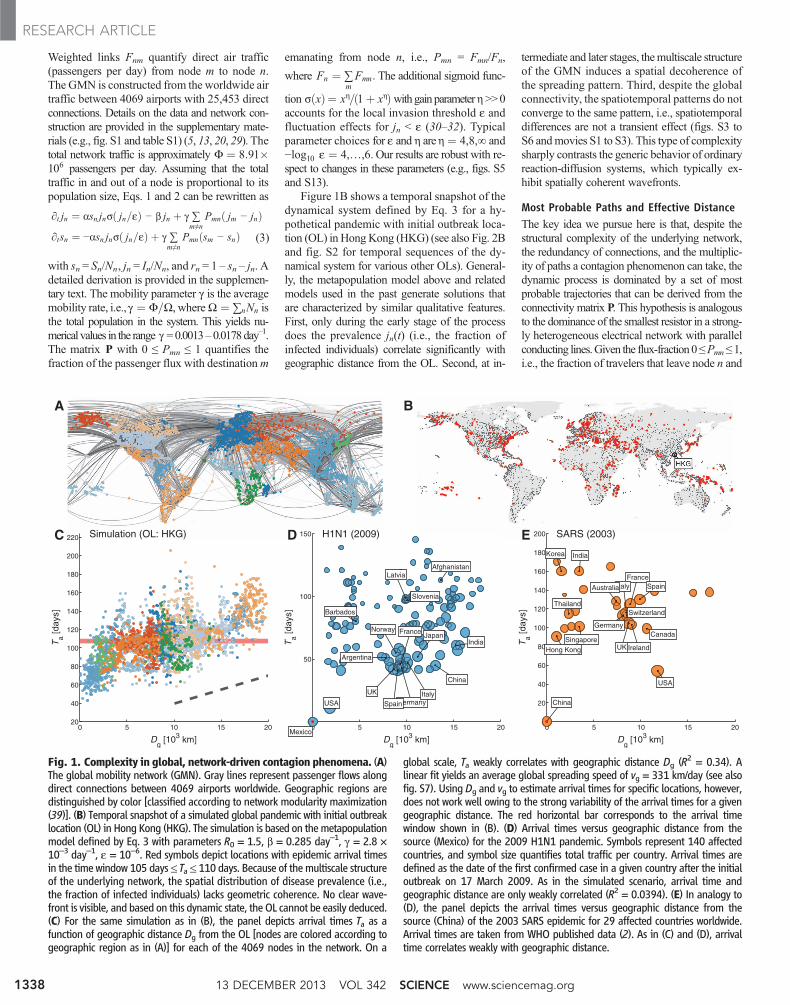
Again, we typically haveDmn ≠ Dnm. Fromthe perspective of a chosen origin node n, the setof shortest paths to all other nodes constitutes ashortest path treeYn (Fig. 2A), illustrating themostprobable sequence of paths from the root node nto the other nodes.

Effective Distance Perspective RevealsHidden Pattern GeometryThe key question is how, compared to the con-ventional geographic representation, the samespreading process evolves on the shortest pathtree. Figure 2B portrays this comparison. We seethat the effective distance representation has no-table advantages: It reveals simple coherent wavefronts, whereas spatiotemporal patterns in geo-graphical space are complex, incoherent, and hard

to understand. This is a generic feature that isrobust against variations in epidemic parametersand true for any choice of the OL (figs. S11 andS12). Using effective distance, one can thus cal-culate the spreading speed and arrival times of adisease, and determine functional relationshipsbetween epidemiological and mobility parameters.The dynamic simplicity in the new representationis much more than just a trivial visual rearrange-ment of the spatiotemporal pattern. Simple prop-agating waves in the new perspective imply thatthe contagion process is dominated by most prob-able paths, as this is the underlying assumption inthe derivation of Eq. 5. Also, effective distanceand the shortest path trees only depend on thestatic mobility matrix P. This implies that, on aspatial scale described by the metapopulationmodel (Eq. 3), the complexity of the spatiotemporalpattern is largely determined by the structure ofthe mobility component in Eq. 3 and not by thenonlinearities or the disease-specific, epidemio-logical rate parameters of the model.

Figure 2C presents the correlation of arrivaltimes Ta with effective distances Deff for the

BA

T=41 d. T=51 d. T=62 d. T=72 d.

0 5 10 15 2020

40

60

80

100

120

140

160

180

200

220C

Deff

T a [day

s]

Simulation (OL: HKG)

0 5 10 15 200

20

40

60

80

100

120

140

160D

Afghanistan

Argentina

Barbados

China

Germany

Algeria

Spain

France

UK

India

ItalyJapan

Zamonia

Mexico

Netherlands

Norway

Slovenia

USA

Deff

T a [day

s]

H1N1 (2009)

0 5 10 15 20 250

20

40

60

80

100

120

140

160

180

200E

Brazil

China

Germany

SpainFrance

UKHong Kong

Italy

Malaysia

Romania

Singapore

Thailand

USA

Viet Nam

Deff

T a [day

s]

SARS (2003)

Fig. 2. Understanding global contagion phenomena using effectivedistance. (A) The structure of the shortest path tree (in gray) from Hong Kong(central node). Radial distance represents effective distance Deff as defined byEqs. 4 and 5. Nodes are colored according to the same scheme as in Fig. 1A. (B)The sequence (from left to right) of panels depicts the time course of a simulatedmodel disease with initial outbreak in Hong Kong (HKG), for the same param-eter set as used in Fig. 1B. Prevalence is reflected by the redness of the symbols.Each panel compares the state of the system in the conventional geographicrepresentation (bottom) with the effective distance representation (top). Thecomplex spatial pattern in the conventional view is equivalent to a homoge-

neous wave that propagates outwards at constant effective speed in the effectivedistance representation. (C) Epidemic arrival time Ta versus effective distanceDeff for the same simulated epidemic as in (B). In contrast to geographic distance(Fig. 1C), effective distance correlates strongly with arrival time (R2 = 0.973), i.e.,effective distance is an excellent predictor of arrival times. (D and E) Linearrelationship between effective distance and arrival time for the 2009 H1N1pandemic (D) and the 2003 SARS epidemic (E). The arrival time data are thesame as in Fig. 1, D and E. The effective distance was computed from the proj-ected global mobility network between countries. As in the model system, weobserve a strong correlation between arrival time and effective distance.

www.sciencemag.org SCIENCE VOL 342 13 DECEMBER 2013 1339

RESEARCH ARTICLE

simulation shown in Fig. 2B. Compared to Fig. 1C,this demonstrates that effective distance generatesa much higher correlation than geographic dis-tance (R2

eff ¼ 0:97 compared to R2geo ¼ 0:34; see

tables S2 and S3 and fig. S12 for more examples).Furthermore, the relationship of Ta and Deff islinear, which means that the effective speed veff =Deff /Ta of the wavefront is a well-defined con-stant. To compare the regression quality, we com-puted the distribution of relative residuals r =dTa/Ta, using effective or geographic distance as aregressor. The ratio of residual variances impliesa more than 50-fold higher prediction quality(table S3 and fig. S13).

Although we have demonstrated the clearlinear functional relationship for simulated, hy-pothetical scenarios of global disease spread, itis crucial to test the validity and usefulness ofthe effective distance approach on empirical data.Figure 2, D and E, depict arrival time versus ef-fective distance on the basis of data for the 2009H1N1 pandemic and the global 2003 SARS epi-demic, respectively (figs. S14 to S16 and table S4).Arrival times are the same as in Fig. 1, D and E,but shown across effective rather than geographicdistances. As the empirical data are available on acountry resolution, we determined the traffic be-tween countries by aggregation to specify a coarse-grained network (GMNc) (189 nodes, 5004 links)and effective distances from the origin locationin each case (see supplementary text for details).

Both the H1N1 and SARS data exhibit a clearlinear relationship between arrival time and ef-fective distance from the source, even thoughadditional factors complicate the spreading ofreal diseases. Fluctuations, effects due to coarsegraining, and errors in arrival-time measurementscan add noise to the system, which increases thescatter in the linear relationship. To address thegeneral validity of the observed effects, we alsoanalyzed data generated by the global epidemicand mobility model (GLEAM) (www.gleamviz.org), a sophisticated epidemic simulation frame-work (21). GLEAM incorporates air transporta-tion and local commuter traffic on a global scale,is fully stochastic, and permits the simulation ofinfectious state–dependent mobility behavior, clin-ical states, antiviral statement, and more. The re-sults of this analysis are shown in figs. S17 toS19 and are consistent with our claims.

Relative Arrival Times Are Independentof Epidemic ParametersOur results reveal an important, approximaterelationship between the system parameters,which can be summarized as follows:

Ta ¼ Deff ðPÞ︸eff : distance

=veff ða,R0,g,eÞ︸eff : speed

ð6Þ

This equation states that arrival times can becomputed with high fidelity based on the ef-

fective distances Deff and effective spreadingspeed veff, and that each factor depends on dif-ferent parameters of the dynamical system. Theepidemiological parameters determine the effec-tive speed, whereas effective distance dependsonly on the topological features of the staticunderlying network, i.e., the matrix P. Whenconfronted with the outbreak of an emergent in-fectious disease, one of the key problems is thatthe disease-specific parameters are typically un-known in the beginning, and simulations basedon plausible parameter ranges typically exhibitsubstantial variability in predicted outcomes.However, Eq. 6 allows us to compute relativearrival times without knowledge of these pa-rameters. If, for example, the outbreak node islabeled k, while n and m are arbitrary nodes,then Ta(n|k)/Ta(m|k) =Deff(n|k)/Deff(m|k). Equa-tion 6 states that the effective speed veff is aglobal property, independent of the mobility net-work and the outbreak location. Thus, irrespec-tive of mobility and OL, one can investigatehow the effective speed depends on rate param-eters of the system.

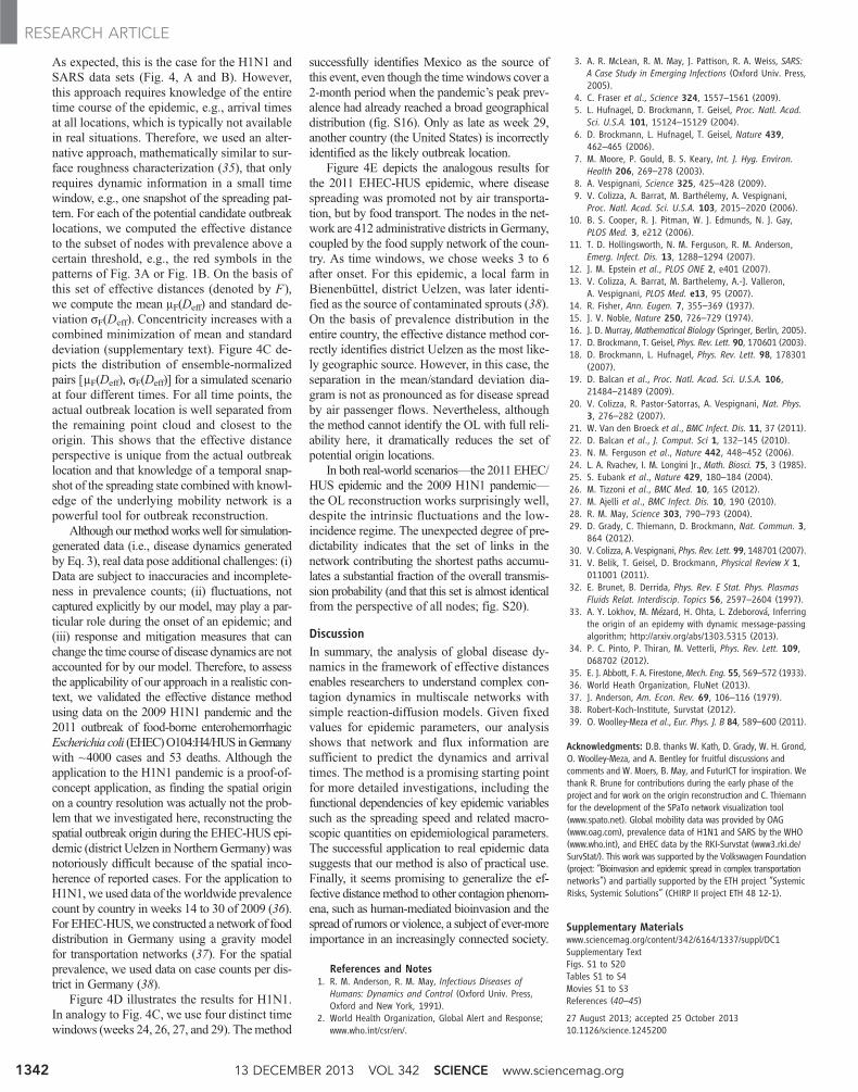
Origin of Outbreak Reconstruction Based onEffective DistanceThe concept of effective distance is particularlyvaluable for solving the aforementioned in-verse problem: Given a spatially distributedprevalence pattern that was generated by an

ALHR

PEK

SYD

ATL

SVO

DXBMEX

YYZ

JNB

HNDBWE

ORD

B

C

DXB

YYZ

BWE

JNB LHR MEX SYD ATL

PEKHNDORDSVO

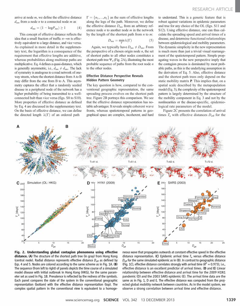
Fig. 3. Qualitative outbreak reconstruction based on effective distance.(A) Spatial distribution of prevalence jn(t) at time T = 81 days for OL Chicago(parameters b = 0.28 day–1, R0 = 1.9, g = 2.8 × 10–3 day–1, and e = 10–6).After this time, it is difficult, if not impossible, to determine the correct OL fromsnapshots of the dynamics. (B) Candidate OLs chosen from different geographicregions. (C) Panels depict the state of the system shown in (A) from the

perspective of each candidate OL, using each OL’s shortest path tree represen-tation. Only the actual OL (ORD, circled in blue) produces a circular wavefront.Even for comparable North American airports [Atlanta (ATL), Toronto (YYZ), andMexico City (MEX)], the wavefronts are not nearly as concentric. Effectivedistances thus permit the extraction of the correct OL, based on information onthe mobility network and a single snapshot of the dynamics.

13 DECEMBER 2013 VOL 342 SCIENCE www.sciencemag.org1340

RESEARCH ARTICLE

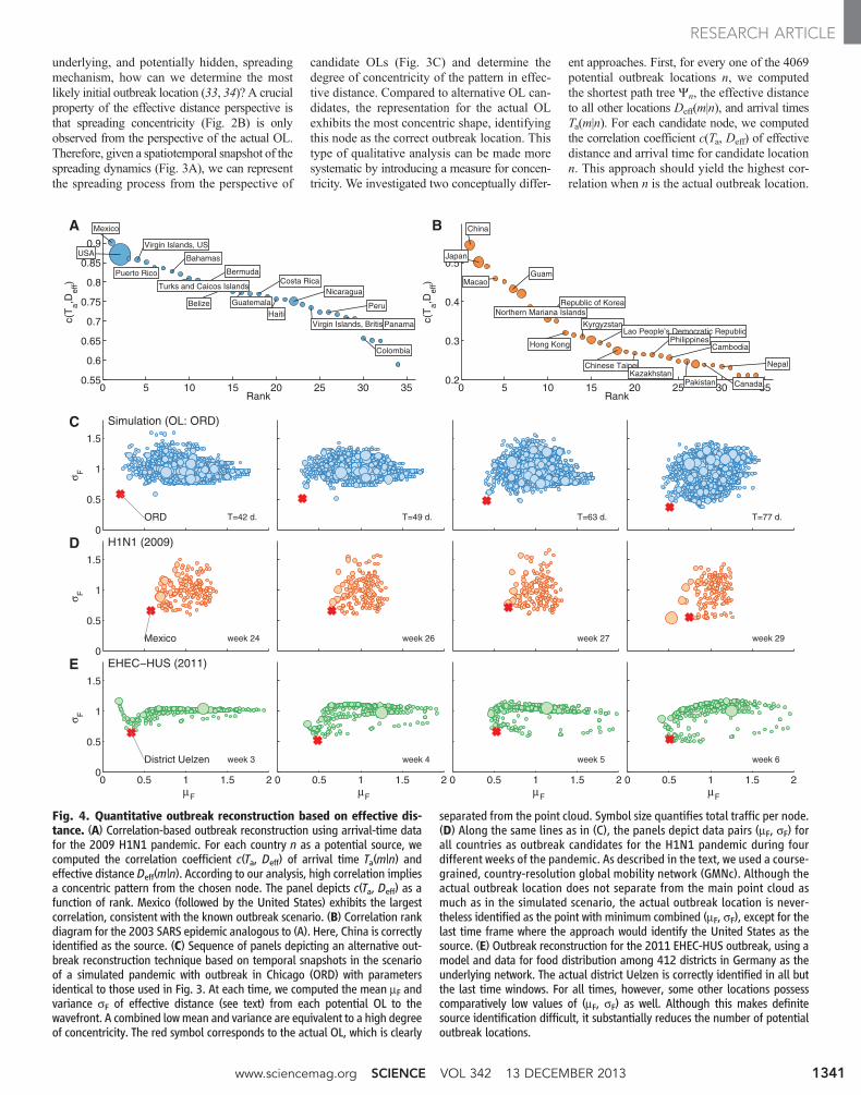
underlying, and potentially hidden, spreadingmechanism, how can we determine the mostlikely initial outbreak location (33, 34)? A crucialproperty of the effective distance perspective isthat spreading concentricity (Fig. 2B) is onlyobserved from the perspective of the actual OL.Therefore, given a spatiotemporal snapshot of thespreading dynamics (Fig. 3A), we can representthe spreading process from the perspective of

candidate OLs (Fig. 3C) and determine thedegree of concentricity of the pattern in effec-tive distance. Compared to alternative OL can-didates, the representation for the actual OLexhibits the most concentric shape, identifyingthis node as the correct outbreak location. Thistype of qualitative analysis can be made moresystematic by introducing a measure for concen-tricity. We investigated two conceptually differ-

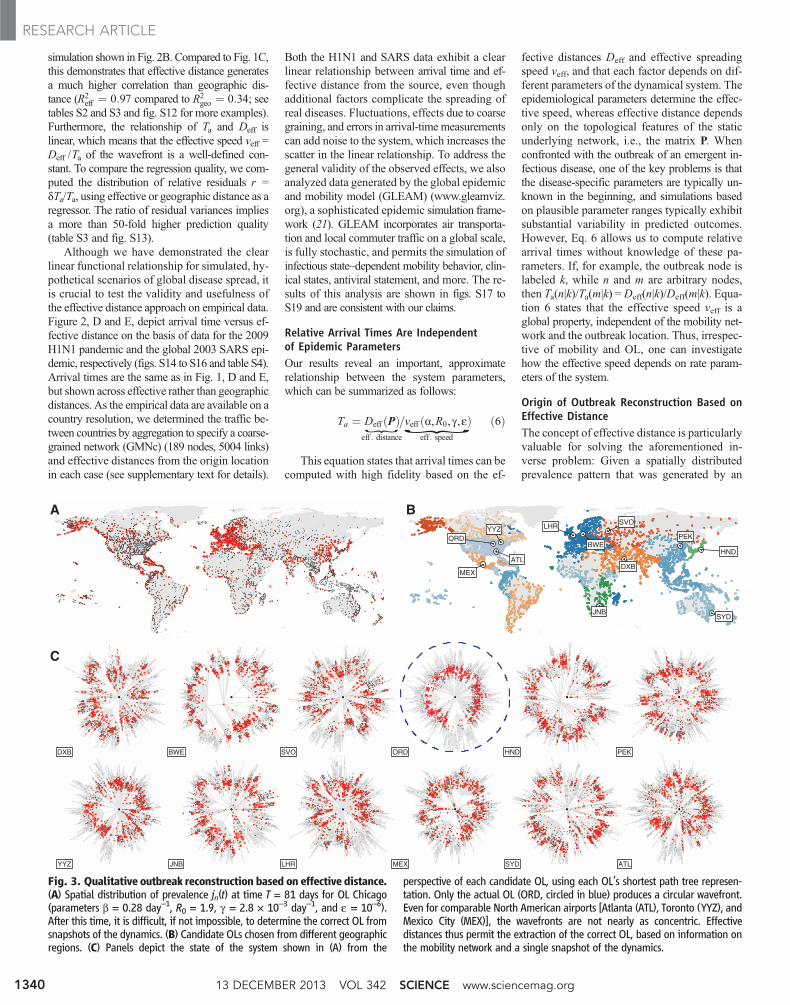
ent approaches. First, for every one of the 4069potential outbreak locations n, we computedthe shortest path tree Yn, the effective distanceto all other locations Deff(m|n), and arrival timesTa(m|n). For each candidate node, we computedthe correlation coefficient c(Ta, Deff) of effectivedistance and arrival time for candidate locationn. This approach should yield the highest cor-relation when n is the actual outbreak location.

0

0.5

1

1.5

ORD T=42 d.

Simulation (OL: ORD)

σ F

T=49 d. T=63 d. T=77 d.

0

0.5

1

1.5

Mexico week 24

H1N1 (2009)

σ F

week 26 week 27 week 29

0 0.5 1 1.5 20

0.5

1

1.5

District Uelzen week 3

EHEC−HUS (2011)

σ F

µF

0 0.5 1 1.5 2

week 4

µF

0 0.5 1 1.5 2

week 5

µF

0 0.5 1 1.5 2

week 6

µF

0 5 10 15 20 25 30 350.55

0.6

0.65

0.7

0.75

0.8

0.85

0.9

Mexico

USAVirgin Islands, US

Puerto Rico

Bahamas

Turks and Caicos Islands

Bermuda

Belize Guatemala

Costa Rica

Haiti

Nicaragua

Virgin Islands, British

Peru

Panama

Colombia

Rank

c(T a,D

eff)

A

0 5 10 15 20 25 30 350.2

0.3

0.4

0.5

China

Japan

MacaoGuam

Northern Mariana IslandsRepublic of Korea

Hong Kong

KyrgyzstanLao People’s Democratic Republic

Chinese TaipeiKazakhstan

PhilippinesCambodia

Pakistan Canada

Nepal

Rank

c(T a,D

eff)

B

C

D

E

Fig. 4. Quantitative outbreak reconstruction based on effective dis-tance. (A) Correlation-based outbreak reconstruction using arrival-time datafor the 2009 H1N1 pandemic. For each country n as a potential source, wecomputed the correlation coefficient c(Ta, Deff) of arrival time Ta(m|n) andeffective distance Deff(m|n). According to our analysis, high correlation impliesa concentric pattern from the chosen node. The panel depicts c(Ta, Deff) as afunction of rank. Mexico (followed by the United States) exhibits the largestcorrelation, consistent with the known outbreak scenario. (B) Correlation rankdiagram for the 2003 SARS epidemic analogous to (A). Here, China is correctlyidentified as the source. (C) Sequence of panels depicting an alternative out-break reconstruction technique based on temporal snapshots in the scenarioof a simulated pandemic with outbreak in Chicago (ORD) with parametersidentical to those used in Fig. 3. At each time, we computed the mean mF andvariance sF of effective distance (see text) from each potential OL to thewavefront. A combined lowmean and variance are equivalent to a high degreeof concentricity. The red symbol corresponds to the actual OL, which is clearly

separated from the point cloud. Symbol size quantifies total traffic per node.(D) Along the same lines as in (C), the panels depict data pairs (mF, sF) forall countries as outbreak candidates for the H1N1 pandemic during fourdifferent weeks of the pandemic. As described in the text, we used a course-grained, country-resolution global mobility network (GMNc). Although theactual outbreak location does not separate from the main point cloud asmuch as in the simulated scenario, the actual outbreak location is never-theless identified as the point with minimum combined (mF, sF), except for thelast time frame where the approach would identify the United States as thesource. (E) Outbreak reconstruction for the 2011 EHEC-HUS outbreak, using amodel and data for food distribution among 412 districts in Germany as theunderlying network. The actual district Uelzen is correctly identified in all butthe last time windows. For all times, however, some other locations possesscomparatively low values of (mF, sF) as well. Although this makes definitesource identification difficult, it substantially reduces the number of potentialoutbreak locations.

www.sciencemag.org SCIENCE VOL 342 13 DECEMBER 2013 1341

RESEARCH ARTICLE

As expected, this is the case for the H1N1 andSARS data sets (Fig. 4, A and B). However,this approach requires knowledge of the entiretime course of the epidemic, e.g., arrival timesat all locations, which is typically not availablein real situations. Therefore, we used an alter-native approach, mathematically similar to sur-face roughness characterization (35), that onlyrequires dynamic information in a small timewindow, e.g., one snapshot of the spreading pat-tern. For each of the potential candidate outbreaklocations, we computed the effective distanceto the subset of nodes with prevalence above acertain threshold, e.g., the red symbols in thepatterns of Fig. 3A or Fig. 1B. On the basis ofthis set of effective distances (denoted by F),we compute the mean mF(Deff) and standard de-viation sF(Deff). Concentricity increases with acombined minimization of mean and standarddeviation (supplementary text). Figure 4C de-picts the distribution of ensemble-normalizedpairs [mF(Deff), sF(Deff)] for a simulated scenarioat four different times. For all time points, theactual outbreak location is well separated fromthe remaining point cloud and closest to theorigin. This shows that the effective distanceperspective is unique from the actual outbreaklocation and that knowledge of a temporal snap-shot of the spreading state combined with knowl-edge of the underlying mobility network is apowerful tool for outbreak reconstruction.

Although ourmethodworkswell for simulation-generated data (i.e., disease dynamics generatedby Eq. 3), real data pose additional challenges: (i)Data are subject to inaccuracies and incomplete-ness in prevalence counts; (ii) fluctuations, notcaptured explicitly by our model, may play a par-ticular role during the onset of an epidemic; and(iii) response and mitigation measures that canchange the time course of disease dynamics are notaccounted for by our model. Therefore, to assessthe applicability of our approach in a realistic con-text, we validated the effective distance methodusing data on the 2009 H1N1 pandemic and the2011 outbreak of food-borne enterohemorrhagicEscherichia coli (EHEC)O104:H4/HUS inGermanywith ~4000 cases and 53 deaths. Although theapplication to the H1N1 pandemic is a proof-of-concept application, as finding the spatial originon a country resolution was actually not the prob-lem that we investigated here, reconstructing thespatial outbreak origin during the EHEC-HUS epi-demic (district Uelzen inNorthernGermany) wasnotoriously difficult because of the spatial inco-herence of reported cases. For the application toH1N1, we used data of the worldwide prevalencecount by country in weeks 14 to 30 of 2009 (36).For EHEC-HUS,we constructed a network of fooddistribution in Germany using a gravity modelfor transportation networks (37). For the spatialprevalence, we used data on case counts per dis-trict in Germany (38).

Figure 4D illustrates the results for H1N1.In analogy to Fig. 4C, we use four distinct timewindows (weeks 24, 26, 27, and 29). Themethod

successfully identifies Mexico as the source ofthis event, even though the time windows cover a2-month period when the pandemic’s peak prev-alence had already reached a broad geographicaldistribution (fig. S16). Only as late as week 29,another country (the United States) is incorrectlyidentified as the likely outbreak location.

Figure 4E depicts the analogous results forthe 2011 EHEC-HUS epidemic, where diseasespreading was promoted not by air transporta-tion, but by food transport. The nodes in the net-work are 412 administrative districts in Germany,coupled by the food supply network of the coun-try. As time windows, we chose weeks 3 to 6after onset. For this epidemic, a local farm inBienenbüttel, district Uelzen, was later identi-fied as the source of contaminated sprouts (38).On the basis of prevalence distribution in theentire country, the effective distance method cor-rectly identifies district Uelzen as the most like-ly geographic source. However, in this case, theseparation in the mean/standard deviation dia-gram is not as pronounced as for disease spreadby air passenger flows. Nevertheless, althoughthe method cannot identify the OL with full reli-ability here, it dramatically reduces the set ofpotential origin locations.

In both real-world scenarios—the 2011 EHEC/HUS epidemic and the 2009 H1N1 pandemic—the OL reconstruction works surprisingly well,despite the intrinsic fluctuations and the low-incidence regime. The unexpected degree of pre-dictability indicates that the set of links in thenetwork contributing the shortest paths accumu-lates a substantial fraction of the overall transmis-sion probability (and that this set is almost identicalfrom the perspective of all nodes; fig. S20).

DiscussionIn summary, the analysis of global disease dy-namics in the framework of effective distancesenables researchers to understand complex con-tagion dynamics in multiscale networks withsimple reaction-diffusion models. Given fixedvalues for epidemic parameters, our analysisshows that network and flux information aresufficient to predict the dynamics and arrivaltimes. The method is a promising starting pointfor more detailed investigations, including thefunctional dependencies of key epidemic variablessuch as the spreading speed and related macro-scopic quantities on epidemiological parameters.The successful application to real epidemic datasuggests that our method is also of practical use.Finally, it seems promising to generalize the ef-fective distancemethod to other contagion phenom-ena, such as human-mediated bioinvasion and thespread of rumors or violence, a subject of ever-moreimportance in an increasingly connected society.

References and Notes1. R. M. Anderson, R. M. May, Infectious Diseases of

Humans: Dynamics and Control (Oxford Univ. Press,Oxford and New York, 1991).

2. World Health Organization, Global Alert and Response;www.who.int/csr/en/.

3. A. R. McLean, R. M. May, J. Pattison, R. A. Weiss, SARS:A Case Study in Emerging Infections (Oxford Univ. Press,2005).

4. C. Fraser et al., Science 324, 1557–1561 (2009).5. L. Hufnagel, D. Brockmann, T. Geisel, Proc. Natl. Acad.

Sci. U.S.A. 101, 15124–15129 (2004).6. D. Brockmann, L. Hufnagel, T. Geisel, Nature 439,

462–465 (2006).7. M. Moore, P. Gould, B. S. Keary, Int. J. Hyg. Environ.

Health 206, 269–278 (2003).8. A. Vespignani, Science 325, 425–428 (2009).9. V. Colizza, A. Barrat, M. Barthélemy, A. Vespignani,

Proc. Natl. Acad. Sci. U.S.A. 103, 2015–2020 (2006).10. B. S. Cooper, R. J. Pitman, W. J. Edmunds, N. J. Gay,

PLOS Med. 3, e212 (2006).11. T. D. Hollingsworth, N. M. Ferguson, R. M. Anderson,

Emerg. Infect. Dis. 13, 1288–1294 (2007).12. J. M. Epstein et al., PLOS ONE 2, e401 (2007).13. V. Colizza, A. Barrat, M. Barthelemy, A.-J. Valleron,

A. Vespignani, PLOS Med. e13, 95 (2007).14. R. Fisher, Ann. Eugen. 7, 355–369 (1937).15. J. V. Noble, Nature 250, 726–729 (1974).16. J. D. Murray, Mathematical Biology (Springer, Berlin, 2005).17. D. Brockmann, T. Geisel, Phys. Rev. Lett. 90, 170601 (2003).18. D. Brockmann, L. Hufnagel, Phys. Rev. Lett. 98, 178301

(2007).19. D. Balcan et al., Proc. Natl. Acad. Sci. U.S.A. 106,

21484–21489 (2009).20. V. Colizza, R. Pastor-Satorras, A. Vespignani, Nat. Phys.

3, 276–282 (2007).21. W. Van den Broeck et al., BMC Infect. Dis. 11, 37 (2011).22. D. Balcan et al., J. Comput. Sci 1, 132–145 (2010).23. N. M. Ferguson et al., Nature 442, 448–452 (2006).24. L. A. Rvachev, I. M. Longini Jr., Math. Biosci. 75, 3 (1985).25. S. Eubank et al., Nature 429, 180–184 (2004).26. M. Tizzoni et al., BMC Med. 10, 165 (2012).27. M. Ajelli et al., BMC Infect. Dis. 10, 190 (2010).28. R. M. May, Science 303, 790–793 (2004).29. D. Grady, C. Thiemann, D. Brockmann, Nat. Commun. 3,

864 (2012).30. V. Colizza, A. Vespignani, Phys. Rev. Lett. 99, 148701 (2007).31. V. Belik, T. Geisel, D. Brockmann, Physical Review X 1,

011001 (2011).32. E. Brunet, B. Derrida, Phys. Rev. E Stat. Phys. Plasmas

Fluids Relat. Interdiscip. Topics 56, 2597–2604 (1997).33. A. Y. Lokhov, M. Mézard, H. Ohta, L. Zdeborová, Inferring

the origin of an epidemy with dynamic message-passingalgorithm; http://arxiv.org/abs/1303.5315 (2013).

34. P. C. Pinto, P. Thiran, M. Vetterli, Phys. Rev. Lett. 109,068702 (2012).

35. E. J. Abbott, F. A. Firestone,Mech. Eng. 55, 569–572 (1933).36. World Heath Organization, FluNet (2013).37. J. Anderson, Am. Econ. Rev. 69, 106–116 (1979).38. Robert-Koch-Institute, Survstat (2012).39. O. Woolley-Meza et al., Eur. Phys. J. B 84, 589–600 (2011).

Acknowledgments: D.B. thanks W. Kath, D. Grady, W. H. Grond,O. Woolley-Meza, and A. Bentley for fruitful discussions andcomments and W. Moers, B. May, and FuturICT for inspiration. Wethank R. Brune for contributions during the early phase of theproject and for work on the origin reconstruction and C. Thiemannfor the development of the SPaTo network visualization tool(www.spato.net). Global mobility data was provided by OAG(www.oag.com), prevalence data of H1N1 and SARS by the WHO(www.who.int), and EHEC data by the RKI-Survstat (www3.rki.de/SurvStat/). This work was supported by the Volkswagen Foundation(project: “Bioinvasion and epidemic spread in complex transportationnetworks”) and partially supported by the ETH project “SystemicRisks, Systemic Solutions” (CHIRP II project ETH 48 12-1).

Supplementary Materialswww.sciencemag.org/content/342/6164/1337/suppl/DC1Supplementary TextFigs. S1 to S20Tables S1 to S4Movies S1 to S3References (40–45)

27 August 2013; accepted 25 October 201310.1126/science.1245200

13 DECEMBER 2013 VOL 342 SCIENCE www.sciencemag.org1342

RESEARCH ARTICLE