The Helioseismologist’s Guide to IRAF

Ed Anderson

Global Oscillation Network GroupNational Solar Observatory

National Optical Astronomy Observatory††

ABSTRACT

The GONG Reduction and Analysis Software Package (GRASP) is a setof tasks designed for helioseismic data analysis. GRASP is a scientificapplications package of, and layered in, the Image Reduction andAnalysis Facility (IRAF), and supported by the GONG project. Alongwith GRASP, many of the generic image processing tasks of IRAF canbe very useful to the helioseismologist and solar astronomer. Manyhelioseismologists may also find some of the optical astronomy tasksuseful to them as well.

This guide is intended to complement A User’s Introduction to theIRAF Command Language (Shames and Tody, 1986) by describing at anintroductory level how to work in the IRAF environment and also pro-vide a broad overview of the generic image processing and analysis taskswithin IRAF.

This guide is large by virtue of examples, and not complexity ordetail of the system it is describing. It is to be used as a first resourcewhich hopefully will point the way into the proper section of the threevolume IRAF manual set if more detail is required.

Revision History:June 1989: First Draft Chapters 1-3 Completed (IRAF 2.7).June 1990: Revised to IRAF 2.9; Chapter 4.1 Added.October, 1990: First Edition Completed (IRAF 2.9).February, 1993: Typos corrected, minor wording changes made.

††Operated by the Association of Universities for Research in Astronomy, Inc. undercooperative agreement with the National Science Foundation.

February 12, 1993

Table of Contents

1. Introduction ...................................................................................................... 1

2. IRAF Basics....................................................................................................... 22.1. Setting Up to Run IRAF ........................................................................ 22.2. Logging into IRAF................................................................................. 32.3. Loading Packages................................................................................... 42.4. Displaying Menus................................................................................... 42.5. Logging Out of IRAF............................................................................. 42.6. The CL as a Command Interpreter ........................................................ 42.7. Using the On-line Help .......................................................................... 62.8. Locating Unknown Tasks....................................................................... 7

2.8.1. IRAF Version 2.8 and Beyond ................................................ 72.8.2. Pre-2.8 Versions....................................................................... 8

2.9. Executing CL Commands and Tasks..................................................... 82.10. Comments About Command Syntax ..................................................... 102.11. Editing Task Parameters......................................................................... 122.12. IRAF File Names ................................................................................... 132.13. IRAF Data Files ..................................................................................... 142.14. Disk Space .............................................................................................. 152.15. IRAF Networking................................................................................... 162.16. Using the Host Operating System.......................................................... 162.17. Advanced CL Usage............................................................................... 17

2.17.1. Session Logging....................................................................... 172.17.2. Background Jobs ...................................................................... 182.17.3. The History Mechanism........................................................... 20

2.18. Miscellaneous ......................................................................................... 212.18.1. The Most Common CL Commands and Tasks....................... 212.18.2. Aborting Tasks (The Non-graceful Exit) ................................ 222.18.3. Where is the Hardware?........................................................... 232.18.4. Setting Terminal Characteristics.............................................. 24

3. Customizing IRAF............................................................................................ 263.1. Operating System Login Files ............................................................... 26

3.1.1. UNIX........................................................................................ 263.1.2. VMS ......................................................................................... 263.1.3. .IRAFHOSTS File.................................................................... 27

3.2. IRAF Login Files ................................................................................... 283.3. Sun Workstation Setup........................................................................... 30

3.3.1. .login......................................................................................... 303.3.2. .defaults .................................................................................... 303.3.3. .ttyswrc ..................................................................................... 313.3.4. .sunview.................................................................................... 32

February 12, 1993

3.4. DECstation Setup ................................................................................... 333.4.1. .X11Startup .............................................................................. 333.4.2. .Xdefaults ................................................................................. 333.4.3. .login and .cshrc ....................................................................... 33

4. Generic Image Processing ............................................................................... 344.1. Getting Data In and Out of IRAF (DATAIO)....................................... 34

4.1.1. General Tape Handling ............................................................ 354.1.1.1. Device Allocation & Deallocation.......................... 354.1.1.2. Tape Density Specification ..................................... 354.1.1.3. Tape positioning...................................................... 36

4.1.2. Textfile I/O............................................................................... 374.1.3. Imagefile I/O ............................................................................ 414.1.4. Dealing With Unknown Tapes ................................................ 434.1.5. Using Exabyte Tapes ............................................................... 46

4.2. Image Display (TV) ............................................................................... 474.2.1. TV.DISPLAY........................................................................... 474.2.2. IMTOOL .................................................................................. 56

4.2.2.1. Frame Buffer Configuration .................................... 564.2.2.2. Executing IMTOOL ................................................ 574.2.2.3. The Frame Menu..................................................... 584.2.2.4. The Setup Panel ...................................................... 584.2.2.5. The Function Keys .................................................. 604.2.2.6. Mouse Buttons......................................................... 614.2.2.7. Hardcopy Output ..................................................... 62

4.2.3. SAOIMAGE............................................................................. 644.2.3.1. Executing SAOIMAGE........................................... 644.2.3.2. Mouse Modes .......................................................... 654.2.3.3. Keyboard Modes ..................................................... 73

4.2.4. Captain Video .......................................................................... 764.2.5. Displaying Images Over the IRAF Network........................... 81

4.3. IRAF Graphics (PLOT).......................................................................... 824.3.1. IMPLOT ................................................................................... 824.3.2. GRAPH .................................................................................... 854.3.3. CONTOUR............................................................................... 894.3.4. SURFACE................................................................................ 904.3.5. HAFTON.................................................................................. 914.3.6. PVECTOR................................................................................ 924.3.7. VELVECT................................................................................ 944.3.8. Cursor Mode ............................................................................ 954.3.9. Hardcopy Output......................................................................1014.3.10. Alternate Cursor Input .............................................................1024.3.11. The Graphics Kernel Tasks .....................................................1034.3.12. Graphics Overlays on the Image Display (IMDKERN) .........106

February 12, 1993

4.4. Image Manipulation (IMAGES) ............................................................1084.4.1. Image Section Notation ...........................................................1094.4.2. Getting Information About an Image ......................................1104.4.3. Preparing Lists of Images ........................................................1184.4.4. Copying, Mosaicing and Deleting Images ..............................1214.4.5. Image Arithmetic .....................................................................1244.4.6. Image Transformations ............................................................1284.4.7. Image Filtering.........................................................................1334.4.8. Edge Detection .........................................................................1374.4.9. Fitting Functions to Images .....................................................1404.4.10. Interactive Curve Fitting (ICFIT) ............................................144

5. The Other IRAF Packages ..............................................................................1515.1. The NOAO Package...............................................................................151

5.1.1. PROTO.....................................................................................1515.1.2. ARTDATA...............................................................................1705.1.3. ASTUTIL .................................................................................1705.1.4. DIGIPHOT ...............................................................................1715.1.5. IMRED .....................................................................................1715.1.6. MTLOCAL...............................................................................1725.1.7. ONEDSPEC .............................................................................1725.1.8. TWODSPEC ............................................................................174

5.2. The LISTS Package................................................................................1745.3. The UTILITIES Package........................................................................1775.4. The SOFTOOLS Package ......................................................................179

February 12, 1993

Table of Examples

This table lists the examples given in the sections on generic image processing.The examples are enumerated in the text by title, in the following format:

Example section.subsection.example_number.

4.1.1. Reading card image tapes to text image disk files ....................................... 374.1.2. Reading card image tapes to text image disk files ....................................... 374.1.3. Reading card image tapes to text image disk files ....................................... 374.1.4. Writing card image tapes............................................................................... 384.1.5. Reading card image tapes.............................................................................. 384.1.6. Writing card image tapes............................................................................... 384.1.7. Converting text image disk files to IRAF images ........................................ 394.1.8. Converting text image disk files ignoring header info ................................. 394.1.9. Converting IRAF images to text image disk files ........................................ 404.1.10. Converting IRAF images to text files with psuedo FITS headers .............. 404.1.11. Converting text files with psuedo FITS headers to IRAF images ............... 404.1.12. Reading card image tape directly into IRAF images ................................... 404.1.13. Reading a FITS tape into IRAF images........................................................ 414.1.14. Reading a FITS tape into IRAF images........................................................ 414.1.15. Listing the contents of a FITS tape............................................................... 414.1.16. Reading FITS disk files across the network ................................................. 424.1.17. Writing a 32-bit FITS tape with long blocks................................................ 434.1.18. Writing a standard FITS tape ........................................................................ 434.1.19. Using mtexamine to determine tape structure ............................................. 444.1.20. Using reblock to correct a byte-swapped FITS file ..................................... 45

4.2.1. Using display with different contrast values................................................ 514.2.2. Using display with zscale and zrange .......................................................... 524.2.3. Using display with different ztrans functions .............................................. 534.2.4. Using display with a user provided color table ........................................... 544.2.5. Using display to mosaic different sized images........................................... 55

4.3.1. Using implot to overplot rows of different images...................................... 844.3.2. Using graph with the lintran option ............................................................ 864.3.3. Using graph to overplot image and list data................................................ 874.3.4. Using graph in point mode with error bars ................................................. 884.3.5. Using contour ............................................................................................... 894.3.6. Using surface ................................................................................................ 904.3.7. Using hafton.................................................................................................. 914.3.8. Using pvector ................................................................................................ 934.3.9. Using pvector saving the vector as an image .............................................. 944.3.10. Using velvect ................................................................................................. 944.3.11. Using cursor mode options to annotate a plot .............................................. 994.3.12. Another demonstration of cursor mode ability .............................................1004.3.13. Using implot with cursor input from a file ..................................................1024.3.14. Using gkiextract outputting to a file ............................................................104

February 12, 1993

4.3.15. Using gkiextract outputting to a hardcopy device.......................................1044.3.16. Using gkimosaic............................................................................................1054.3.17. Using imdkern to overlay contour plot on the image display.....................1064.3.18. Using contour to plot directly to the image display ....................................107

4.4.1. Using image sections.....................................................................................1094.4.2. Using image sections.....................................................................................1094.4.3. Using image sections.....................................................................................1094.4.4. Using imheader to list the short header.......................................................1104.4.5. Using imheader to list the long header........................................................1104.4.6. Using imheader to list the long header........................................................1114.4.7. Using imstatistics..........................................................................................1124.4.8. Using imstatistics..........................................................................................1124.4.9. Using imhistogram .......................................................................................1134.4.10. Using minmax...............................................................................................1144.4.11. Using minmax...............................................................................................1144.4.12. Using imgets..................................................................................................1154.4.13. Using hedit to append to the image title interactively.................................1164.4.14. Using hedit to append to the image title noninteractively...........................1164.4.15. Using hedit to edit headers based on a header keyword value....................1174.4.16. Using listpixels to examine an image section ..............................................1184.4.17. Using listpixels piping result to graph ........................................................1184.4.18. Using files to generate an image list .............................................................1194.4.19. Using files to generate an image list .............................................................1194.4.20. Using files to generate an image list .............................................................1194.4.21. Using sections to determine the number of images .....................................1204.4.22. Using sections to generate input and output lists.........................................1204.4.23. Using hselect to generate a list of images....................................................1204.4.24. Using hselect to generate a list of images....................................................1214.4.25. Using imcopy to copy images to a new directory........................................1224.4.26. Using imcopy to trim images .......................................................................1224.4.27. Using imcopy to mosaic images into one image .........................................1224.4.28. Using imrename to move images to a different directory...........................1224.4.29. Using imrename to move image pixels to a different directory .................1224.4.30. Using chpixtype to convert images to a different datatype .........................1234.4.31. Using chpixtype to convert images to a different datatype .........................1234.4.32. Using imdelete ..............................................................................................1234.4.33. Using imarith ................................................................................................1254.4.34. Using imarith ................................................................................................1254.4.35. Using imcombine ..........................................................................................1274.4.36. Using imcombine ..........................................................................................1274.4.37. Using imdivide ..............................................................................................1274.4.38. Using imshift.................................................................................................1284.4.39. Using imshift to register images...................................................................1284.4.40. Using imrotate ..............................................................................................1294.4.41. Using imrotate to rotate about a specified pixel..........................................1294.4.42. Using imstack ...............................................................................................130

February 12, 1993

4.4.43. Using imslice .................................................................................................1304.4.44. Using geomap noninteractively ....................................................................1324.4.45. Using geomap to register images .................................................................1334.4.46. Using imlintrans to apply a linear transformation ......................................1334.4.47. Using blkavg on an image cube ...................................................................1344.4.48. Using blkrep .................................................................................................1344.4.49. Median filter an image...................................................................................1364.4.50. Median filter an image...................................................................................1364.4.51. Median filter an image...................................................................................1364.4.52. Convolve and image with a user specified kernel ........................................1374.4.53. Convolve and image with a user specified kernel ........................................1374.4.54. Using the gradient edge detector .................................................................1384.4.55. Using the laplace edge detector....................................................................1394.4.56. Using fit1d noninteractively..........................................................................1414.4.57. Using lineclean noninteractively ..................................................................1414.4.58. Using imsurfit ...............................................................................................1434.4.59. Using fit1d interactively................................................................................146

5.1.1. Using fields to extract columns from a text file ...........................................1535.1.2. Using fields to extract columns from a text file ...........................................1515.1.3. Using join to produce a multi-column text file ............................................1515.1.4. Using interp to interpolate tabular data .......................................................1545.1.5. Using interp to generate a smooth curve for overplotting ..........................1555.1.6. Using mkhistogram ......................................................................................1565.1.7. Using tvmark with autolog=yes ..................................................................1585.1.8. Using tvmark to annotate an l−ν diagram ...................................................1595.1.9. Using epix to edit image pixels ....................................................................1615.1.10. Using epix to edit image pixels ....................................................................1615.1.11. Using fixpix to clean bad pixel regions ........................................................1625.1.12. Using imexamine ..........................................................................................166

5.2.1. Using columns to break up a text table........................................................1755.2.2. Using lintran to tranform a list of coordinates ............................................176

February 12, 1993

1. Introduction

The IRAF system provides a large selection of programs for general image pro-cessing and graphics applications, and a suite of programs for reduction and analysis ofoptical astronomy data. In particular the GONG Reduction and Analysis SoftwarePackage (GRASP) of IRAF will provide the software tools specific to helioseismic dataprocessing.

Four basic parts make up the run-time IRAF system:� The Command Language (CL) provides the user interface to the system,� The Applications Packages contain the data analysis programs for specific

science applications (e.g., the GRASP package) and generic image processingand plotting utilities (e.g., the IMAGES and PLOT packages),

� The Virtual Operation System (VOS) supports the portability of the system,� The Host System Interface (HSI) is the interface between the portable IRAF

system and a particular host system.

The general user only needs to be concerned with the first two parts.

IRAF provides its own environment (i.e., its own operating system, the VOS) fromwhich the CL operates, and some new users may be reluctant to learn yet anotheroperating system. The advantage of learning IRAF far outweighs the perceived disad-vantage of learning another system, in that the user is now machine independent and assuch can move from one site to another, one machine to another, and collaborate withpeople at different computing sites, without having to learn new commands, syntax, etc.GONG DMAC (Data Management and Analysis Center) visitors may return to theirhome institutions and continue data analysis using the same software and the sameoperating environment but on completely different computer hardware.

In addition to supplying various suites of image processing programs, IRAF pro-vides the user with ways to hook external programs (written by the user or someoneelse) into the user’s IRAF environment.

As previously mentioned, this guide complements, not replaces the CL User’sGuide. The author assumes that the reader is familiar with the first four chapters of theCL User’s Guide and will only summarize the more important items from thosechapters in the next section of this document.

In addition, this guide presents a broad overview of the generic image processingand analysis tools within IRAF. To that end, this document is the Reader’s DigestAbridged Version of the three volume (six binder) IRAF documentation set. Indeed,much of the task-specific discussion is taken verbatim (with details left out) from therelevant help pages, and hence the author is more of an editor than creative author.Much of what is in this document was written in part by all members of the IRAF pro-gramming group.

This document is large (circa 180 pages) by virtue of the large number of exam-ples included, as opposed to presenting detailed specifics about each item. It is hoped,that the general user may find this document a useful starting point for learning thehows and wheres of various tasks. Should more detailed documentation be required,then the task help pages, and IRAF cookbooks will need to be consulted.

February 12, 1993

2

2. IRAF Basics

This section briefly reviews some of the more important basics of how to set upand use IRAF. All of the topics discussed here are documented in greater detail in theCL User’s Guide and/or the on-line help facility.

2.1. Setting Up to Run IRAF

IRAF is generally run from a subdirectory of the user’s root directory. This isNOT a requirement, but it does serve to separate one’s IRAF files from whatever elseone might have. Thus, the steps required to set up the IRAF environment are:

1. Create an IRAF login directory. It is suggested that the name of this sub-directory be IRAF. For example, on a UNIX system the command would be:

% mkdir iraf

On a VMS system, this command would be:

$ create/dir [.iraf]

2. Go to that directory.

3. Enter the command:

mkiraf

The system will respond by asking for the type of terminal being used. Oneshould answer with the type that will be most often used (e.g., vt640). One isnot restricted to using that type of terminal when logged into IRAF as the ter-minal type can be interactively reset from the CL (see §2.18.4).

Among the many actions the mkiraf command performs, is the creation of a filecalled LOGIN.CL and a subdirectory called UPARM.

� The LOGIN.CL file is read by IRAF when logging into the CL. Analogous to the.login file on a UNIX system or the login.com file on a VMS system, this file con-tains a number of environment declarations, and may be edited to customize theuser’s IRAF environment.

� The UPARM subdirectory is where IRAF stores the user parameters for any ofthe IRAF tasks that one executes. This enables IRAF to prompt with the answersfrom a previous execution of a particular task and also enables one to customizethe parameters of any task to suit one’s needs.

It is NOT necessary to use the mkiraf command before every IRAF session. However,one might want to use it to reinitialize one’s IRAF environment periodically. The com-mand may be required when a major IRAF system update has been performed.

February 12, 1993

3

NOTE: On VMS systems it may be necessary to enter the command IRAF todefine the system symbolic names for IRAF (of which mkiraf is one), asmany system managers will not define the IRAF global symbols at logintime. For further discussion, see §3.1.2.

NOTE: If, on UNIX systems, the response to mkiraf is an error message sayingthat the command is not found, check that the search path includes theproper directories. Current UNIX configurations will usually install theIRAF symbols and links in /local/bin or /usr/local/bin. Check with the sys-tem manager if problems remain.

2.2. Logging into IRAF

To log into IRAF (start the CL) first go to your IRAF directory and then enter thecommand:

cl

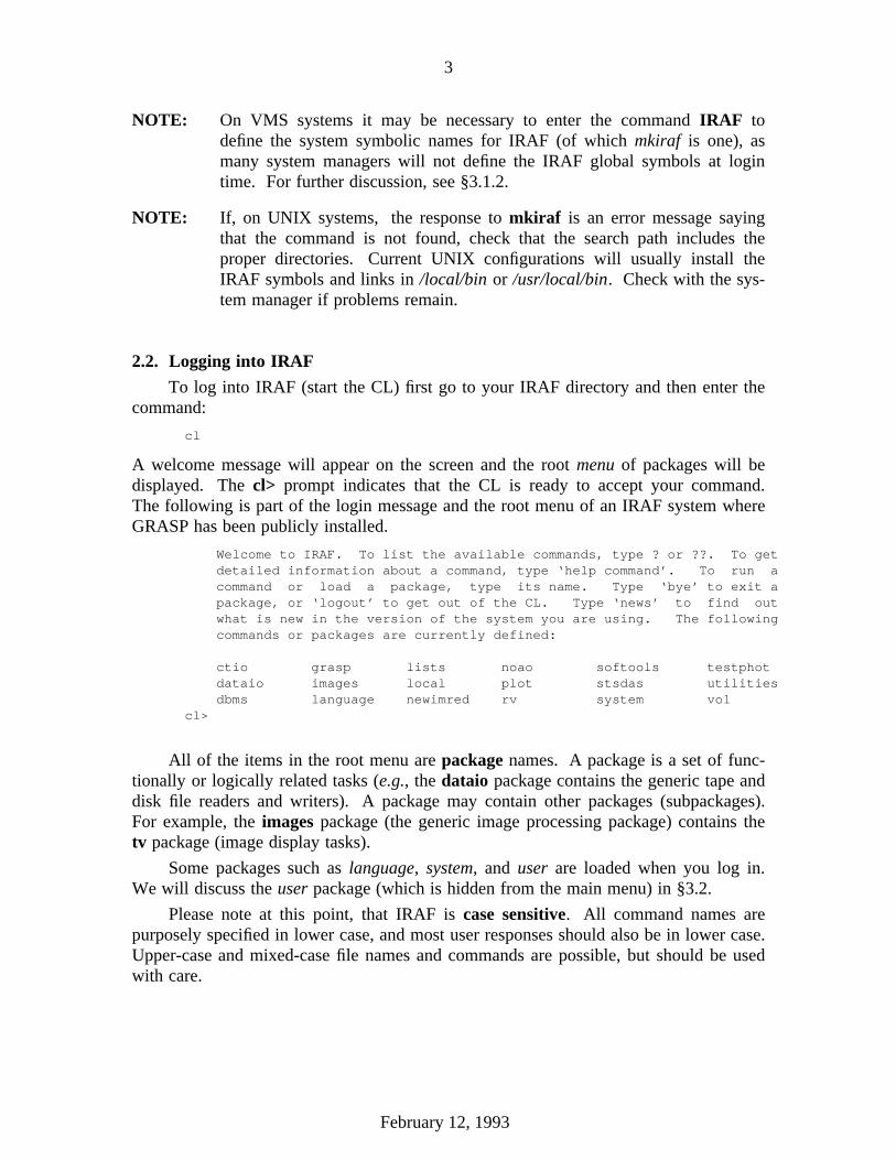
A welcome message will appear on the screen and the root menu of packages will bedisplayed. The cl> prompt indicates that the CL is ready to accept your command.The following is part of the login message and the root menu of an IRAF system whereGRASP has been publicly installed.

Welcome to IRAF. To list the available commands, type ? or ??. To getdetailed information about a command, type ‘help command’. To run acommand or load a package, type its name. Type ‘bye’ to exit apackage, or ‘logout’ to get out of the CL. Type ‘news’ to find outwhat is new in the version of the system you are using. The followingcommands or packages are currently defined:

ctio grasp lists noao softools testphotdataio images local plot stsdas utilitiesdbms language newimred rv system vol

cl>

All of the items in the root menu are package names. A package is a set of func-tionally or logically related tasks (e.g., the dataio package contains the generic tape anddisk file readers and writers). A package may contain other packages (subpackages).For example, the images package (the generic image processing package) contains thetv package (image display tasks).

Some packages such as language, system, and user are loaded when you log in.We will discuss the user package (which is hidden from the main menu) in §3.2.

Please note at this point, that IRAF is case sensitive. All command names arepurposely specified in lower case, and most user responses should also be in lower case.Upper-case and mixed-case file names and commands are possible, but should be usedwith care.

February 12, 1993

4

2.3. Loading Packages

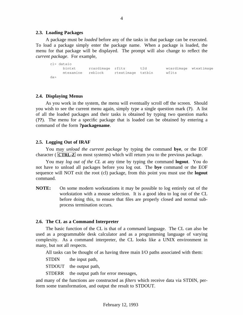
A package must be loaded before any of the tasks in that package can be executed.To load a package simply enter the package name. When a package is loaded, themenu for that package will be displayed. The prompt will also change to reflect thecurrent package. For example,

cl> dataiobintxt rcardimage rfits t2d wcardimage wtextimagemtexamine reblock rtextimage txtbin wfits

da>

2.4. Displaying Menus

As you work in the system, the menu will eventually scroll off the screen. Shouldyou wish to see the current menu again, simply type a single question mark (?). A listof all the loaded packages and their tasks is obtained by typing two question marks(??). The menu for a specific package that is loaded can be obtained by entering acommand of the form ?packagename.

2.5. Logging Out of IRAF

You may unload the current package by typing the command bye, or the EOFcharacter ( CTRL-Z on most systems) which will return you to the previous package.

You may log out of the CL at any time by typing the command logout. You donot have to unload all packages before you log out. The bye command or the EOFsequence will NOT exit the root (cl) package, from this point you must use the logoutcommand.

NOTE: On some modern workstations it may be possible to log entirely out of theworkstation with a mouse selection. It is a good idea to log out of the CLbefore doing this, to ensure that files are properly closed and normal sub-process termination occurs.

2.6. The CL as a Command Interpreter

The basic function of the CL is that of a command language. The CL can also beused as a programmable desk calculator and as a programming language of varyingcomplexity. As a command interpreter, the CL looks like a UNIX environment inmany, but not all respects.

All tasks can be thought of as having three main I/O paths associated with them:

STDIN the input path,

STDOUT the output path,

STDERR the output path for error messages,

and many of the functions are constructed as filters which receive data via STDIN, per-form some transformation, and output the result to STDOUT.

February 12, 1993

5

� Task input through STDIN may be accepted from a file (input redirection) with acommand of the form,

task < inputfile

� Task output through STDOUT may be redirected to a file with a command of theform:

task > outputfile

or

task >> outputfile

where ">" redirects output to a new file, and ">>" appends output to an existingfile or creates the file if it does not exist.

� Task output through STDOUT may be piped to the input of another task with acommand of the form,

task1 | task2

If executing a task with verbose output, or in background, or batch, one mightwant to redirect STDERR and STDOUT to a file (or separate files) for later checking.The command is of the form,

task > outfile >& errorfile

Like output redirection, one may also use ">>&" to append to files.

One may combine the above to make quite sophisticated command strings withouthaving to deal with intermediate files. For example,

task1 < infile >>& errfile | task2 >>& errfile | task3 >>& errfile > outfile

There are three other output streams in IRAF:

STDGRAPH the graphics terminal (or device) stream,

STDPLOT the graphics plotter device,

STDIMAGE the image display device.

In your usage of IRAF, you will encounter tasks which output to one of these streams.Like the other I/O streams, these may also be redirected. The graphics stream isredirected with the operators >G or >>G, the STDPLOT stream may be redirected withthe operators >P, of >>P, and the STDIMAGE stream with >I or >>I. Examples ofredirecting these streams are given in examples 4.3.13-15.

As a final note, you might wish to run a task that uses several output streams, butonly want to keep the output from one of those streams. IRAF provides a bit-bucket ornull-file called dev$null to which any of the output streams may be redirected.

February 12, 1993

6

2.7. Using the On-line Help

Usually, the package and task names are sufficient to inform the user what thatparticular package or task does. If, however, you would like more information, an on-line help facility is available.

Asking for help for a package will result in a display of the task and subpackagenames with a one-line synopsis of what each task does. For example, to get help forthe current package one simply enters the command help. The following is the helpsummary for the clpackage (i.e., the root package).

cl> helpdataio - Data format conversion package (RFITS, etc.)

dbms - Database management package (not yet implemented)images - General image processing package

language - The command language itselflists - List processing packagelocal - Local (site dependent) tasks and packagesnoao - The NOAO optical astronomy packagesplot - Plot package

softools - Software tools packagesystem - System utilities package

utilities - Miscellaneous utilities package

To get a summary for a particular package type help packagename. For example:

cl> help system

system.:allocate - Allocate a device, e.g., magtape drive mta, mtb, ...

concatenate - Concatenate a list of filescopy - Copy a file or files (use IMCOPY for imagefiles)count - Count the number of lines, words, characters in a text file

deallocate - Deallocate a previously allocated devicedelete - Delete a file or files (use IMDELETE to delete imagefiles)devices - Print information on the locally available devices

devstatus - Print the status of a device (mta, mtb, ...)directory - List the files in a directorydiskspace - Show how much diskspace is available

files - Expand a file template into a list of filesgripes - Send suggestions, complaints, etc. to the system

head - Print the first few lines of a text filehelp - Print online documentation

lprint - Print a file on the line printer devicematch - Print all lines in a file that match a patternmkdir - Create a new directory

mkscript - Make a command scriptmovefiles - Move files to a directorynetstatus - Print the status of the local network

news - Page through the system news filepage - Page through a file

pathnames - Expand a file template into a list of OS pathnamesprotect - Protect a file from deletion

references - Find all help database references for a given topicrename - Rename a filerewind - Rewind a device (magtape)sort - Sort a text filespy - Show processor statustail - Print the last few lines of a file

February 12, 1993

7

tee - Tee the standard output into a filetype - Type a text file on the standard output

unprotect - Remove delete protection from a file

To get detailed help for a particular task, type help taskname. For example,

cl> help sort

will display the help page for the task sort.

Should you wish a hardcopy of the help page(s), then you could enter theappropriate help command and pipe the output to the print command. For example,

cl> help sort | lprint

will print out the help pages for the sort task on the user’s default printer.†

NOTE: It is not necessary to have the package loaded in order to see the help pagefor a particular task of that package. The help files for the current packageare searched first and if no match is found, then the remainder of the helpdatabase is searched.

The reader is strongly encouraged to read the help pages for help which containother useful features which have not been discussed here.

2.8. Locating Unknown Tasks

This section describes how to locate a task of unknown name. For example, whatif I want to use a task that reads and writes binary files.

2.8.1. IRAF Version 2.8 and Beyond

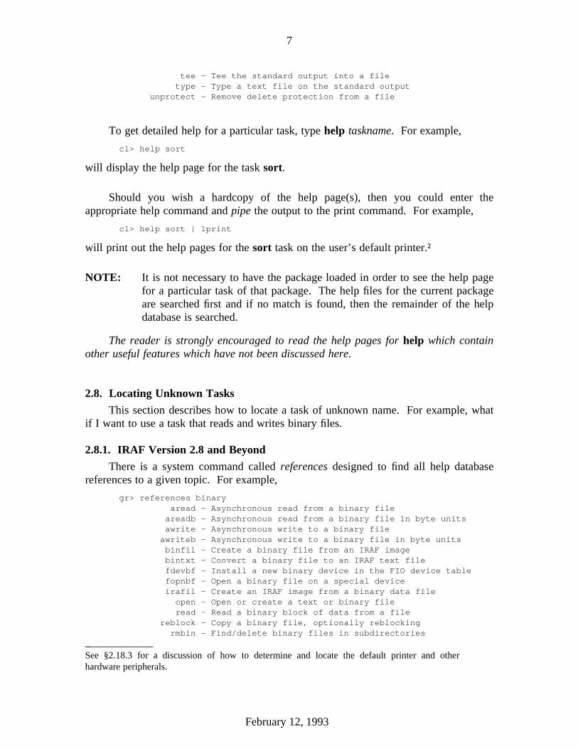
There is a system command called references designed to find all help databasereferences to a given topic. For example,

gr> references binaryaread - Asynchronous read from a binary file

areadb - Asynchronous read from a binary file in byte unitsawrite - Asynchronous write to a binary fileawriteb - Asynchronous write to a binary file in byte unitsbinfil - Create a binary file from an IRAF imagebintxt - Convert a binary file to an IRAF text filefdevbf - Install a new binary device in the FIO device tablefopnbf - Open a binary file on a special deviceirafil - Create an IRAF image from a binary data fileopen - Open or create a text or binary fileread - Read a binary block of data from a file

reblock - Copy a binary file, optionally reblockingrmbin - Find/delete binary files in subdirectories

See §2.18.3 for a discussion of how to determine and locate the default printer and otherhardware peripherals.

February 12, 1993

8

txtbin - Convert an IRAF text file to a binary filewrite - Write a binary block of data to a file

From such a list, you may then ask for help for a specific task(s) which will theninform you what packages to load in order to use that task. Not all tasks in this list areavailable to the interactive user; some of them will be subroutines provided for applica-tions programming.

2.8.2. Pre-2.8 Versions

For pre-2.8 Versions of IRAF, one may use the help command to request help fora template of characters which you might think would be in the task name. The on-linehelp facility accepts templates of the form

package_pattern.task_pattern

where the standard pattern-matching metacharacters "*?[]" are permitted. If the dot(".") is not present then help assumes that the template is of a task. For example, if youare looking for a task that deals with binary files, you could try a command of the form,

cl> help *.*bin*

which will search all the package help files for a task with the character string "bin" inits name. Among the dozen or so matches would be dataio.bintxt, dataio.txtbin andnoao.proto.binfil.

However, there might be other tasks that work on binary files, but do not have thestring "bin" in their names. An alternative search is to ask for help on just the packagesonly, and search for lines containing the word "binary". Since in this case the packagemenus are searched, you will not have to deal with the actual help pages themselves.For example the command,

cl> help *. | match "binary" | page

produces the same result as the references command of Version 2.8.

2.9. Executing CL Commands and Tasks

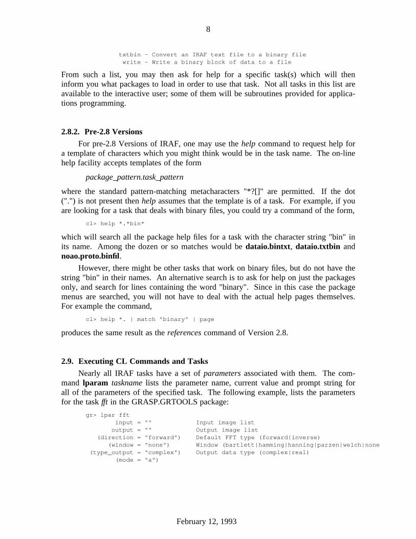
Nearly all IRAF tasks have a set of parameters associated with them. The com-mand lparam taskname lists the parameter name, current value and prompt string forall of the parameters of the specified task. The following example, lists the parametersfor the task fft in the GRASP.GRTOOLS package:

gr> lpar fftinput = "" Input image list

output = "" Output image list(direction = "forward") Default FFT type (forward|inverse)

(window = "none") Window (bartlett|hamming|hanning|parzen|welch|none(type_output = "complex") Output data type (complex|real)

(mode = "a")

February 12, 1993

9

� The first parameters to be listed (i.e., those not enclosed in parentheses) are thepositional or queried parameters. These are the parameters that the task abso-lutely must have in order to execute. If you do not supply these parameters viathe command line, the task will ask you for them using the listed prompts.

� The second set of parameters (i.e., those that are enclosed in parentheses) are hid-den parameters. The task uses the values shown unless the user explicitly changesthose values on the command line or prior to execution with the parameter editor.

The form of the command required to execute an IRAF task is simply the taskname itself, optionally followed by an argument or parameter list. The followingexamples show variations of how one might execute the fft task of the above example.The first example shows the interaction that takes place when only the taskname isgiven:

gr> fftInput image list: testOutput image list: ffttestgr>

Since no arguments were supplied, the task queried for the necessary input and outputfile name parameters. The values of the hidden parameters are those listed above.

Most IRAF tasks use the CL facility called learn mode by default. This is denoted bythe parameter mode with a value of "a" (automatic) or "ql" (query and learn) in thelparam output. Any time a task is used in a manner where the user must be queried,the task will prompt with the previous answers (if any). For example,

gr> fftInput image list (test):Output image list (ffttest): fftest2gr>

If the prompted answer is correct, one need only type RETURN , otherwise one mayenter a new answer to the query.

It is not necessary to play the query-and-answer game when executing tasks.More often than not, you will know what the task is looking for. You can enter thecommand with the positional parameters given on the command line. For example,

gr> fft test ffttest3

Note, that the positional parameters must be given in the order that they appear in theparameter listing.

Should you wish to run a task, with one of the hidden parameters changed tosomething other than the default (or set) value, then you may specify that change with aparameter=value argument on the command line. For example,

gr> fft test ffttest4 window=parzen

Users may change the default values of hidden parameters to customize a particular taskto suit their needs. See §2.11 for details on how to do this.

February 12, 1993

10

For boolean parameters, you may use the param=[yes/no] notation, or alterna-tively you may use param[+-]. For example, to delete all non-image files, with theparameter verify=yes, enter the command:

cl> delete * verify+

You may also run a command in "query mode" while changing hidden parametervalues.

gr> fft direction=inverse type_output=realInput image list (test): ffttest4Output image list (ffttest): inv_test4gr>

Remember that the CL allows abbreviation of all package, task and parameternames to the extent that the abbreviation contains sufficient characters to uniquely iden-tify the name. The last example could have been entered as:

gr> fft d=i t=r

It is suggested that you avoid abbreviation to the point where you no longer recognizethe name yourself.

Other ways of modifying parameter values will be discussed in §2.11.

2.10. Comments About Command Syntax

The following comments are included here for the sake of completeness. Much ofwhat follows applies to more complex usages of the CL, for example, large scripts.

� Different CL commands can be put on the same command line by separating eachcommand with a semicolon character ‘;’. For example,

cl> clear; images; dir

clears the screen, loads the images package, and displays the files in the currentdirectory.

� If the tasks you want to string together will not fit on a single command line youmay also form a compound statement by using the curly braces ‘{}’. The aboveexample could equally have been done as follows:

cl> {>>> clear>>> images>>> dir>>> }

where the prompt changes to >>> after the left brace is entered signaling that theCL is waiting for more input (in particular the right brace ‘}’).

February 12, 1993

11

� Sometimes you will enter a command where you are changing hidden parametersand find that it will not all fit on one line. The command may be continued on thenext line by using a backslash ‘\’ as the last item on the current line. For example,

gr> mkspec test 0. 0.05 12 peak.dat background=100. \>>> title="test spectrum" \>>> tsave+ treal+ option=power

� Note the use of quotes in the above example. Single or double quotes may beused around any string of characters, but in general are not required during interac-tive sessions at the terminal. Quotes need not be used when:

1. the string appears as an identifier (name) in an argument list not enclosed inparentheses,

or

2. the string does not contain any white space, or special characters.

Notice that the above example has white space in the string.

� If the argument list is in parentheses, then the CL will interpret the command incompute or program mode, where unquoted strings are assumed to be variables.For example, consider the CL integer variable j.

cl> j=100cl> print jjcl> print ’j’jcl> print (’j’)jcl> print (j)100

In the first three of the above print commands, the j was treated as a string. In thelast command, the value of the variable j was printed.

� Comment statements may be freely embedded anywhere in the command line. Acomment is delimited by the character ‘#’ and everything on the line after thatcharacter is considered to be part of the comment. For example,

cl> # This is a commentcl> grasp # Load the grasp package

Although comments are used more often in scripts, you might find that commentsare useful in interactive sessions if you are logging your session (see §2.17.1 fordiscussion of session logging).

February 12, 1993

12

2.11. Editing Task Parameters

Sometimes you will want to run a task many times with one or many of the hid-den parameters changed from their default values. In such a case, much time and typ-ing can be saved by changing the hidden parameter values prior to execution. There aretwo ways to change the values of hidden parameter.

The first way is to use a command of the form,

taskname.parametername=newvalue

For example, to set the fft task to always use the parzen window, change the parameterwindow to parzen as follows:

gr> fft.window=parzen

Note that another way to find the current value of a parameter is to use the = command.For example,

gr> =fft.windowparzen

The above method could require a lot of commands should you wish to change anumber of hidden parameters. Also, some tasks such as grasp.mftables.sgraph willhave a number of different parameter sets (psets) associated with the task. In thesecases one should use the parameter editor which is invoked with a command of theform,

eparam taskname

The parameters of taskname will be displayed as shown in the following example (eparfft):

I R A FImage Reduction and Analysis Facility

PACKAGE = grtoolsTASK = fft

input = Input image listoutput = Output image list(directi= forward) Default FFT type (forward|inverse)(window = none) Window (bartlett|hamming|hanning|parzen|welch|none(type_ou= complex) Output data type (complex|real)(mode = a)

The return key will move the cursor down the list or the cursor keys (i.e., arrowkeys) may be used to move among the parameters. Any entries that are typed willreplace the displayed values when the return key is hit. A CTRL-Z may be used atany time to exit eparam updating the task parameters with any changes you have made.A CTRL-C may be used to exit eparam without updating the parameters.

The parameter editor allows switching from one task’s pset to that of another taskby using a colon command option. A colon command may be entered when the cursoris positioned at the starting column of any parameter. To change to the next task enterthe colon command:

February 12, 1993

13

:e next_taskname

which will automatically update the current task parameters before moving on to thenext task. To edit the parameters of another task without updating the current parame-ter set, use the command:

:e! next_taskname.

Execution of the task may also be initiated from within eparam by using the com-mand :go.

Should you find yourself always editing parameters for a particular task then youmight wish to reset the mode of that task so that eparam will be called automatically,each time the task is executed (i.e., menu mode). For example, the command:

gr> fft.mode="ml"

will set both menu and learn mode for the task fft. When exiting eparam (either withCTRL-Z or CTRL-C , the task will automatically execute. As mentioned earlier,the default mode for mode tasks is "ql" (query and learn) or equivalently "a"(automatic).

As with the help task, the reader in urged to read the help pages for eparam inorder to become familiar with all of its features.

Note: To reset task parameters back to the IRAF system defaults, enter the com-mand:

cl> unlearn taskname

2.12. IRAF File Names

IRAF uses virtual file names so that all file and directory references will look thesame on any computer. In general, either the IRAF file name or the operating-system-dependent file name are acceptable to any command but users are encouraged to onlyuse the IRAF file names.

File-name mapping does not operate automatically on virtual file names that arepassed as parameters to foreign (host system) tasks. However, the operating-system-dependent filename is easily found by using the CL function osfn or the system taskpathname. For example, your login.cl file resides in your IRAF home directory.

cl> pathname home$login.cllacerta!/u2/anderson/iraf/login.clcl>cl> =osfn(’home$login.cl’)/u2/anderson/iraf/login.cl

Note that pathname also includes the network node name.

In the above example home is an environment variable set in your login.cl file.Such environment variables play a crucial role in IRAF virtual filenames. To display

February 12, 1993

14

the value of an environment variable, use the show command. For example,

gr> show home/u2/anderson/iraf/

To list all the environment variables defined, just type show with no arguments. Notethat you might want to pipe the output to page.

The full virtual filename is made up of two parts: the logical directory and thespecific filename within that directory. In the virtual filename home$login.cl, the homefield, delimited by a ‘$’ character is the logical directory, and login.cl, the specific file.Names such as home$uparm/ which end with a ‘/’ are directory references. There are anumber of environment variables that the user may set at login time. These will be dis-cussed in §3.2.

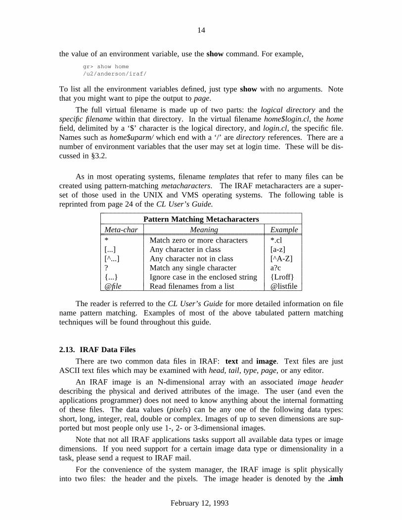
As in most operating systems, filename templates that refer to many files can becreated using pattern-matching metacharacters. The IRAF metacharacters are a super-set of those used in the UNIX and VMS operating systems. The following table isreprinted from page 24 of the CL User’s Guide.

Pattern Matching MetacharactersMeta-char Meaning Example* Match zero or more characters *.cl[...] Any character in class [a-z][^...] Any character not in class [^A-Z]? Match any single character a?c{...} Ignore case in the enclosed string {Lroff}@file Read filenames from a list @listfile

The reader is referred to the CL User’s Guide for more detailed information on filename pattern matching. Examples of most of the above tabulated pattern matchingtechniques will be found throughout this guide.

2.13. IRAF Data Files

There are two common data files in IRAF: text and image. Text files are justASCII text files which may be examined with head, tail, type, page, or any editor.

An IRAF image is an N-dimensional array with an associated image headerdescribing the physical and derived attributes of the image. The user (and even theapplications programmer) does not need to know anything about the internal formattingof these files. The data values (pixels) can be any one of the following data types:short, long, integer, real, double or complex. Images of up to seven dimensions are sup-ported but most people only use 1-, 2- or 3-dimensional images.

Note that not all IRAF applications tasks support all available data types or imagedimensions. If you need support for a certain image data type or dimensionality in atask, please send a request to IRAF mail.

For the convenience of the system manager, the IRAF image is split physicallyinto two files: the header and the pixels. The image header is denoted by the .imh

February 12, 1993

15

extension on the root filename and resides in the user’s directory. The pixel file has a.pix extension and resides in the user’s image directory, which is usually on somescratch disk that is normally volatile and doesn’t get backed up. This prevents usersfrom clogging the home directory disks of the computers with megabytes of pixels. Tosee where the pixels are going, enter the command show imdir.

Note that it is not necessary to specify the .imh extension to tasks that are expect-ing image names as arguments or parameters.

Note also that there are other supported image formats, like the Space Telescopeformat (.stf) and the new Quick Photon Ordered Event format (.qp), but these formatsare not used in the GONG software.

2.14. Disk Space

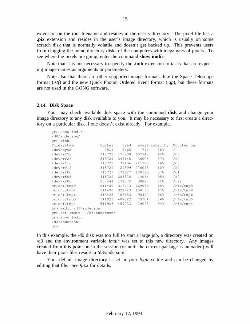
Your may check available disk space with the command disk and change yourimage directory to any disk available to you. It may be necessary to first create a direc-tory on a particular disk if one doesn’t exist already. For example,

gr> show imdir/d0/anderson/gr> diskFilesystem kbytes used avail capacity Mounted on/dev/xy0a 7511 5965 794 88% //dev/rf2g 315729 176209 107947 62% /d5/dev/rf2f 315729 248148 36008 87% /d4/dev/rf1g 315729 78434 221508 26% /d3/dev/rf1f 315729 29899 270043 10% /d2/dev/rf0g 315729 171627 128315 57% /d1/dev/rf0f 315729 285878 14064 95% /d0/dev/xy0g 237444 174872 38827 82% /usrorion:/tmp9 511430 316773 169085 65% /nfs/tmp9orion:/tmp8 511430 327723 158135 67% /nfs/tmp8orion:/tmp6 313423 186653 95427 66% /nfs/tmp6orion:/tmp5 511923 407022 79304 84% /nfs/tmp5orion:/tmp4 511923 457233 29093 94% /nfs/tmp4gr> mkdir /d3/andersongr> set imdir = /d3/anderson/gr> show imdir/d3/anderson/gr>

In this example, the /d0 disk was too full to start a large job, a directory was created on/d3 and the environment variable imdir was set to this new directory. Any imagescreated from this point on in the session (or until the current package is unloaded) willhave their pixel files reside in /d3/anderson/.

Your default image directory is set in your login.cl file and can be changed byediting that file. See §3.2 for details.

February 12, 1993

16

2.15. IRAF Networking

IRAF provides its own networking facility so that various machines at the samesite (e.g., NOAO) can share files, tape drives, image displays, printers, etc.

When IRAF networking is used, a kernel server process is started under the user’sid on the remote machine. In order to start this process, IRAF needs to know the user’spassword on that machine. There are two ways in which IRAF obtains the password.

� First, the system searches for a file called .irafhosts in the user’s login directory.This is a highly protected file containing the user’s passwords to the variousmachines on the local IRAF network. See §3.1.3 for details on how to set up thisfile.

� If the .irafhosts file is not found, the system will query the user. This is doneonly for the first time that a given process is started on the remote machine. Forexample first doing a directory on the remote machine will cause IRAF to queryfor a password. If later, a copy or some other system package command is exe-cuted, then a password will not be required. If an imcopy is requested, a new ker-nel server for the images package would need to start up, and the user wouldagain be queried for a password.

The kernel server will stay in place as long as users do not flush the local processfrom their cache (see §2.18.2 for discussion of flprcache).

2.16. Using the Host Operating System

There will be times when you will want to use a command or facility from thehost operating system because such a facility might not exist within IRAF or perhapsyou are more familiar with your host system. It is not necessary to log out of the CL inorder to execute a host level command. Any command may be sent to the host systemby escaping that command with the character ‘!’. The remainder of the command lineis passed, unmodified, to the host system. An example of this would be,

gr> !mail

When the operating-system task has completed you will be back in the CL.

Sometimes there might be problems executing a complicated host-level command.Such problems usually occur on VMS operating systems where subprocesses do notinherit the full environment of the parent process. See your local IRAF or operatingsystem wizard if problems arise.

If IRAF networking is implemented, then the user may execute host-level com-mands on a remote host in a similar fashion to using the rsh command in UNIX. Theform of the command is:

!remote_hostname!command[; command ....]

For example,

cl> !aquila!cd iraf/mydata; ls -l

February 12, 1993

17

2.17. Advanced CL Usage

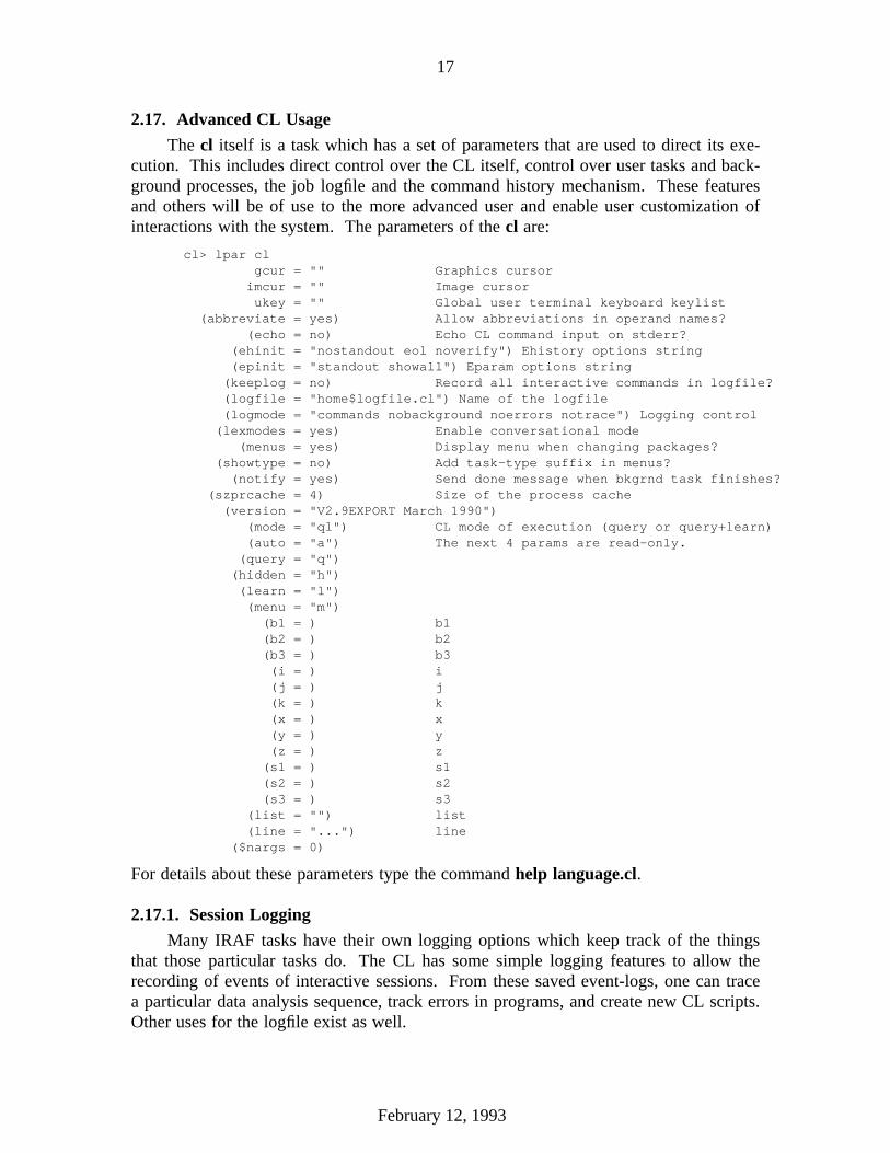
The cl itself is a task which has a set of parameters that are used to direct its exe-cution. This includes direct control over the CL itself, control over user tasks and back-ground processes, the job logfile and the command history mechanism. These featuresand others will be of use to the more advanced user and enable user customization ofinteractions with the system. The parameters of the cl are:

cl> lpar clgcur = "" Graphics cursorimcur = "" Image cursorukey = "" Global user terminal keyboard keylist

(abbreviate = yes) Allow abbreviations in operand names?(echo = no) Echo CL command input on stderr?

(ehinit = "nostandout eol noverify") Ehistory options string(epinit = "standout showall") Eparam options string(keeplog = no) Record all interactive commands in logfile?(logfile = "home$logfile.cl") Name of the logfile(logmode = "commands nobackground noerrors notrace") Logging control(lexmodes = yes) Enable conversational mode

(menus = yes) Display menu when changing packages?(showtype = no) Add task-type suffix in menus?

(notify = yes) Send done message when bkgrnd task finishes?(szprcache = 4) Size of the process cache

(version = "V2.9EXPORT March 1990")(mode = "ql") CL mode of execution (query or query+learn)(auto = "a") The next 4 params are read-only.

(query = "q")(hidden = "h")(learn = "l")(menu = "m")

(b1 = ) b1(b2 = ) b2(b3 = ) b3(i = ) i(j = ) j(k = ) k(x = ) x(y = ) y(z = ) z

(s1 = ) s1(s2 = ) s2(s3 = ) s3

(list = "") list(line = "...") line

($nargs = 0)

For details about these parameters type the command help language.cl.

2.17.1. Session Logging

Many IRAF tasks have their own logging options which keep track of the thingsthat those particular tasks do. The CL has some simple logging features to allow therecording of events of interactive sessions. From these saved event-logs, one can tracea particular data analysis sequence, track errors in programs, and create new CL scripts.Other uses for the logfile exist as well.

February 12, 1993

18

There are currently five types of logging messages, with a parameter to controlwhat is actually logged. These are:

commands - commands and keystrokes of an interactive sessionbackground - messages about and from background jobserrors - logging of error messagestrace - start/stop trace of script and executable tasksuser - user messages, via the putlog builtin

All of these types of messages except the interactive commands will show up as com-ments (i.e., starting with a #) in the logfile. This facilitates using a previous logfile asinput to the CL or as the basis for a script task.

The CL parameters discussed below are used to control the logging features.These parameters can be set on the command line, in the login.cl file, or with the com-mand eparam cl.

keeplogWhen this switch is set to yes, the logfile will be opened and logging willcommence. If the named logfile does not exist, it will be created, otherwiselog messages will be appended to the existing file.

logfileThis is the name of the log file (default home$logfile).

logmodeThis controls what goes into the logfile. The options are:

[no]commands Logging of interactive commands.[no]background Background logging (start/stop messages, etc).[no]errors Error logging within script and executable tasks.[no]trace Tracing of script and executable tasks (start/stop, times, package).

The default is logmode = "commands nobackground noerrors notrace"

Type help language.logging for more information.

2.17.2. Background Jobs

Many image reduction and analysis schemes are very time consuming and neednot be run interactively. IRAF allows such functions to be developed interactively andthen processed in a batch mode as a background task, thus freeing the terminal for otherinteractions once the background tasks have been started, or even allowing the user tolog off. Several background tasks can be running at once, and these may be identicaltasks that are just operating on different data sets.

Any command, including compound commands that may involve calls to severaltasks, may be executed in the background by appending the ampersand character & tothe end of the command block. The CL will create a new control process for the back-ground job, start it, display the job number of the background job, and return control tothe terminal. Background job numbers are always small integers in the range 1 to n,where n is the maximum permissible number of background jobs (typically 3-6). Forexample,

February 12, 1993

19

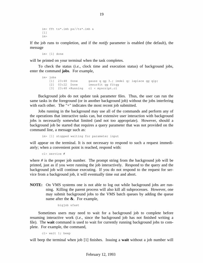
im> fft ts*.imh ps//ts*.imh &[1]im>

If the job runs to completion, and if the notify parameter is enabled (the default), themessage

im> [1] done

will be printed on your terminal when the task completes.

To check the status (i.e., clock time and execution status) of background jobs,enter the command jobs. For example,

im> jobs[1] 23:48 Done gauss q qg 3.; imdel q; laplace qg qlp;[2] 03:22 Done imsurfit qg fitqg[3] 23:48 +Running cl < myscript.cl

Background jobs do not update task parameter files. Thus, the user can run thesame tasks in the foreground (or in another background job) without the jobs interferingwith each other. The "+" indicates the most recent job submitted.

Jobs running in the background may use all of the commands and perform any ofthe operations that interactive tasks can, but extensive user interaction with backgroundjobs is necessarily somewhat limited (and not too appropriate). However, should abackground job be started that requires a query parameter that was not provided on thecommand line, a message such as:

im> [1] stopped waiting for parameter input

will appear on the terminal. It is not necessary to respond to such a request immedi-ately; when a convenient point is reached, respond with:

cl> service #

where # is the proper job number. The prompt string from the background job will beprinted, just as if you were running the job interactively. Respond to the query and thebackground job will continue executing. If you do not respond to the request for ser-vice from a background job, it will eventually time out and abort.

NOTE: On VMS systems one is not able to log out while background jobs are run-ning. Killing the parent process will also kill all subprocesses. However, onemay submit background jobs to the VMS batch queues by adding the queuename after the &. For example,

bigjob &fast

Sometimes users may need to wait for a background job to complete beforeresuming interactive work (i.e., since the background job has not finished writing afile). The wait command is used to wait for currently running background jobs to com-plete. For example, the command,

cl> wait 1; beep

will beep the terminal when job [1] finishes. Issuing a wait without a job number will

February 12, 1993

20

cause the interactive session to wait for all background jobs to complete.

Background jobs may be aborted by issuing a kill command. For example, thecommand to abort job [1] would be,

cl> kill 1

2.17.3. The History Mechanism

The CL history mechanism keeps a record of the commands you enter and pro-vides a way of reusing commands to invoke new operations with a minimum of typing.The history mechanism should not be confused with the logfile; the history mechanismdoes not make a permanent record of commands, and the logfile cannot be used to savetyping (except by using the editor on it after the end of the session). With the historyeditor, previous commands can easily be edited to correct errors, without the need toretype the entire command.

The history n command is used to display n previous command lines (default n is15). For example,

im> history 3103 disp vmi[*,*,3] 3 fill+ or=2104 imcopy vmi[*,*,2] mod105 lpar imedit

Note, that this number n will become the new default. If a negative number of com-mands (-n) is specified, the default will not change.

The command ehistory allows the user to re-execute, or to edit and execute, com-mands. Once in the the history editor, the cursor (arrow) keys can be used to moveabout in the history file. You may select any command and edit it using the simple editcommands described previously for eparam.

It is possible to recall individual commands and edit them; the special character ˆor the ehistory command may be used for this. Given the history record sequenceshown above, any of the following commands could be used to fetch command 103:

cl> ˆ103 # fetch and execute command 103cl> ehist -3 # fetch and edit the 3rd last command [103]cl> ˆdi # fetch and execute 103cl> ehist ?fill? # fetch and edit 103

The history command ˆdi finds the last command beginning with the string "di", whilethe command ehist ?fill? finds the last command containing the string "fill" (the trailing"?" is optional if it is the last character on the line). A single ˆ fetches the last commandentered.

In editing a command, the selected command is echoed on the screen, with thecursor pointing at it. At that point, the command can be executed just by typingRETURN , or it may be edited.

Sometimes you will want to reuse the arguments of a previous command. Thenotation "ˆˆ" refers to the first argument of the last command entered, "ˆ$" refers to thelast argument of the command, "ˆ" refers to the whole argument list, "ˆ0" refers to thetaskname of the last command, and "ˆN" refers to argument N of the last commandentered. Thus, the command sequence

February 12, 1993

21

cl> dir lib$*.h,home$login.clcl> lprint ^^

displays a table of the files specified by the template, and then prints the same files onthe line printer.

One of the most useful features of the history mechanism is the ability to repeat acommand with additional arguments appended. Any recalled command may be fol-lowed by some extra parameters, which are appended to the command. For example,

ut> urand 200 2 | graph point+ut> ˆˆ title="200 random numbers"urand 200 2 | graph point+ title="200 random numbers"

In this case, the notation (ˆˆ) refers to the last command entered. Note, the notation isunambiguous because it appears at the start of the command line.

A command of the form "ˆstring:p" finds the last command beginning with thestring string and puts in at the end of the history stack (i.e., makes it the last command)without executing. This allows one to edit the command as if it were the previous com-mand (as described in the preceding paragraph). For example,

cl> disp raw 1cl> median raw medraw 3 3cl> ^disp:pdisp raw 1cl> ^^ xc=.25; disp medraw 1 xc=.75 er-

2.18. Miscellaneous

2.18.1. The Most Common CL Commands and Tasks

The following table lists the most common CL commands that the user needs toknow about. Items in the list are found in either the language or system packages (notall tasks in these packages are listed) and are therefore available immediately uponstarting the CL.

access - Test if a file existsback - Return to the previous directory (after a chdir)beep - Send a beep to the terminalbye - Exit a task or packagecd - Change directory

chdir - Change directoryclear - Clear the terminal screenedit - Edit a text file

eparam - Edit parameters of a taskflprcache - Flush the process cache

logout - Log out of the CLlparam - List the parameters of a task

osfn - Return the host system equivalent of an IRAF filenamereset - Reset the value of an environment variable

set - Set an environment variableshow - Show an environment variablestty - Set/show terminal characteristicstime - Print the current time

unlearn - Restore the default parameters for a task or package

February 12, 1993

22

update - Update a task’s parameters (flush to disk)

concatenate - Concatenate a list of filescopy - Copy a file or files (use IMCOPY for imagefiles)count - Count the number of lines, words, characters in a text file

delete - Delete a file or files (use IMDELETE to delete imagefiles)devices - Print information on the locally available devices

directory - List the files in a directorydiskspace - Show how much diskspace is available

head - Print the first few lines of a text filehelp - Print online documentation

lprint - Print a file on the line printer devicematch - Print all lines in a file that match a patternmkdir - Create a new directory

movefiles - Move files to a directorynews - Page through the system news filepage - Page through a file

pathnames - Expand a file template into a list of OS pathnamesprotect - Protect a file from deletionrename - Rename a filesort - Sort a text filespy - Show processor statustail - Print the last few lines of a filetee - Tee the standard output into a file

type - Type a text file on the standard outputunprotect - Remove delete protection from a file

All of the tasks that display, copy, delete or move files, apply to non-image files only.The images package provides a separate set of tasks to operate on images (See §4.4 fora discussion of the images package).

2.18.2. Aborting Tasks (The Non-graceful Exit)

There will be times when having typed the wrong command, or realizing that atask is taking too long to execute that you will want to abort execution. To abort anytask execution, enter the command CTRL-C .

There are a few tricks to using the CTRL-C abort. The first is to realize that byvirtue of IRAF’s operating system independence, trapping CTRL-C interrupts on vari-ous systems has proved to be difficult if not frustrating.

� If a CTRL-C is entered immediately after the RETURN for a task, then some-times the CL will hang.

Wait for the task to get loaded. If the task is going to query, wait until the firstquery before using CTRL-C .

� There is a fair amount of error recovery required during a CTRL-C abort. If youhit CTRL-C many times in succession, the latter CTRL-C’s will be passed to thehost operating system, and result in a panic abort of the subprocess, sometimes tothe extent that the CL itself is aborted.

Only do one CTRL-C, and then wait a few seconds to see if IRAF aborts the taskgracefully or not.

February 12, 1993

23

� To make things memory efficient and to minimize disk I/O, IRAF caches execut-able images in the user’s memory workspace. To see what executables arecurrently in the process cache, enter the command prcache with no arguments.For example,

tv> prc[13] lacerta!2247(8C7X) H bin$x_display.e[10] lacerta!2246(8C6X) H bin$x_plot.e[04] lacerta!2245(8C5X) H bin$x_images.e[05] lacerta!2169(879X) HL bin$x_system.e

The default process cache size is 3 or 4, but can be set to a maximum of 10.

CTRL-C aborting during task execution may corrupt the cached executable, andthus may cause an error during the next execution. To prevent this, the usershould flush the process cache by typing the command flpr. For example,

tv> flprprctv> [05] lacerta!2169(879X) HL bin$x_system.e

000

Using flpr with no arguments will cause all idle subprocesses to be flushed fromthe process cache. It is possible to flush specific processes, and the user is referredto the help page for flprcache for details.

2.18.3. Where is the Hardware?

In §2.7 there was a discussion about piping the output of help to your defaultprinter. For many users (especially those at NOAO) there are a number of printers, andtape drives scattered around the building.

� To determine what printer is currently the default, enter the command showprinter

� To determine what printer is currently the default for plot hardcopies, enter thecommand show stdplot

� To determine, where on the site a particular peripheral device is located enter thecommand devices. The following is the listing for NOAO:

DEVICES (Jun89) NOAO/Tucson Device Information DEVICES (Jun89)

Device Aliases Description+Location

lw1 apl|lw Laserwriter, Rm B-50lw2 apl2 Laserwriter, Xerox Rm (Rm 135)lw3 apl3 Laserwriter, Engineering Mezzaninelw4 apl4 Laserwriter, GONG lab (B-14)lw5 apl5|nlw Laserwriter NT, Rm 72lw7 apl7|tops Laserwriter, Solar Office, Rm 152imagen i240 240 dpi imagen, Rm 105

February 12, 1993

24

imagend i300 300 dpi imagen, Rm 113versatec vup|ver Versatec V-80, fan-fold, Rm 72calcomp ccp Calcomp pen plotter, Rm 101vmsprint vmslp VMS cluster lineprinter, Rm 101lpr Direct output to Unix ‘lpr’ program*

*This device is available on UNIX systems only. A specific outputdevice may be selected by defining PRINTER in the user environment.

The following devices can be specified as shown with a trailing ‘s’to indicate a finer linewidth will be used, intended for small, denseplots: lw1s, lw2s, lw3s, lw4s, lw5s, lw7s, i240s, i300s.

tucana!mta [1600|6250]* Fujitsu 1/2" tapedrive, Rm B-50tucana!mtb [4|9] Sun QIC 1/4" cartridge, Rm B-50orion!mta [1600|6250] Fujitsu 1/2" tapedrive, Rm 101orion!mtb [1600|6250] Fujitsu 1/2" tapedrive, Rm 101gemini!mta [1600|6250] Fujitsu 1/2" tapedrive, Rm 101gemini!mtb [?] Exabyte, Rm 101gemini!mtc [?] Sun 1/4" cartridge, Rm 101aquila!mta [1600] DEC TU80 1/2" tapedrive, Rm B-49aquila!mtb [1600|6250] Kennedy 1/2" tapedrive, Rm B-49aquila!mtc [1600|6250] Kennedy 1/2" tapedrive, Rm B-49noao!mta [1600|800] Kennedy 1/2" tapedrive, Rm 101noao!mtb [1600|800] Kennedy 1/2" tapedrive, Rm 101draco!mta [1600|6250] TU78 1/2" tapedrive, Rm 101 [DRACO/VELA only]draco!mtb [1600|6250] TU78 1/2" tapedrive, Rm 101 [DRACO/VELA only]draco!mtc [1600|800]+ Kennedy 1/2" tapedrive, Rm 101 [DRACO only]draco!mtd [1600|800]+ Kennedy 1/2" tapedrive, Rm 101 [DRACO only]draco!mte [1600] TS11 1/2" tapedrive, Rm B-49 [VELA only]draco!mtg [1600|800]+ Kennedy 1/2" tapedrive, Rm 101 [DRACO only]draco!mth [1600|6250] TU78 1/2" tapedrive, Rm 101 [DRACO/VELA only]

*Default tape densities listed first.+The Kennedy drives on VMS nodes do not have a default density;the density must be set manually with the switch on the tape drive.

Should such a listing not be available at your site, contact your IRAF systemmanager.

2.19. Setting Terminal Characteristics

The task stty is used to set or display the terminal device characteristics and VOSterminal driver options. Without arguments, stty prints the current characteristics of theterminal. For example

cl> sttygterm ncols=80 nlines=54

The most common use of stty is to inform IRAF of the type of terminal beingused. For example

cl> stty vt100

would set the terminal type to "vt100". An error message will be printed unless anentry for the named terminal is present in the termcap file; if the named terminal is agraphics terminal, there must also be an entry in the graphcap file.

February 12, 1993

25

Note: The default termcap and graphcap files are dev$termcap and dev$graphcap.Users may provide their own cap files and use them by setting the environ-ment variables termcap and graphcap to point to the correct files (e.g.,reset termcap = home$.termcap ).

The default terminal type can be changed by setting ttyname. The terminal charac-teristics ncols, nlines or baud, may be changed by typing new values explicitly on thecommand line.

There are a number of other options with stty which allow the user to log terminalinput and/or output and also to playback the logfile (useful for demonstration software).Type help stty for more information.

February 12, 1993

26

3. Customizing IRAF

This section briefly discusses how to customize your IRAF environment both atthe operating sytem level and within IRAF itself. Where possible, examples will begiven for both UNIX and VMS operating systems. The last subsection in this discus-sion is concerned specifically with running IRAF on a Sun Workstation.

3.1. Operating System Login Files

3.1.1. UNIX

On UNIX systems, all IRAF related commands should be available immediatelyupon login provided the proper system directories are included in the user’s search path.As mentioned in §2.1, current UNIX configurations usually install the IRAF links in/local/bin or /usr/local/bin.

The only other thing to be concerned about is that the biff command (i.e., biff=yesinforms you when new mail has arrived) must go in the .login, not the .cshrc file. Oth-erwise, the IRAF networking between machines is interrupted.

Once logged into the CL, one may work from any directory, however it is impor-tant that the CL be started from the home IRAF directory. In the .cshrc one coulddefine an alias of the form

alias goiraf ’cd /u2/anderson/iraf; cl’

Entering the command goiraf will result in changing directories to the home IRAFdirectory and logging in to the CL.

3.1.2. VMS

As mentioned in §2.1 of this document, many VMS sites do not define the IRAFlogicals and global symbols at login time. Thus at many sites, users must either typethe command IRAF before logging into the CL or must have the line

$ IRAF

in their login.com file. If such a command is necessary, then it is required to be in thelogin.com if the user is going to run IRAF in VMS batch queues.

Similar to the UNIX example above, it is possible to set up a VMS command filethat will set the default directory to the home IRAF directory and start up the CL. Firstedit a file in your system home directory called say goiraf.com which would looksomething like the following:

$! GOIRAF - Go to home IRAF directory and start the CL$$ set def usr0:[anderson.iraf]$ cl$ exit

In your login.com add a global symbol definition,

February 12, 1993

27

$goiraf :== @usr0:[anderson]goiraf

There is a disadvantage with loading IRAF in such a fashion in that a sub-process slotis used up executing the goiraf command file. The command file does not exit until onehas logged out of the CL. This could be a major problem on heavily used systems.

Alternatively, we recommend the definition of a global symbol in the login.comwhich sets the default to the proper directory only, leaving the starting of the CL to theuser. For example,

$goiraf :== set def usr0:[anderson.iraf]

3.1.3. .irafhosts File

This file is for users who employ the IRAF networking facilities (see §2.15 fordiscussion of IRAF networking). At some sites (e.g., NOAO) this file may be neces-sary. The .irafhosts file resides in your login directory (i.e., the operating system homedirectory), regardless of where the IRAF home directory is located.

The format of the file is,

machine_name : username password

where there is one line in the file for each machine you have an account on. If theusername and password are the same on all machines, then the .irafhosts file need onlybe one line, with an asterisk (∗ ) for the machine name.

Because this file contains your password, it should be protected against anyonereading it.

On VMS systems use the command,

set prot=(s,o:r,g,w) .irafhosts;

On UNIX systems use the command,

chmod 400 .irafhosts

If you are worried about putting your password in a file, the password field can bereplaced by a question mark (?), in which case IRAF will query for your passwordwhen it needs access to another machine (only one query per machine per IRAF ses-sion). Note, however, that VMS batch jobs will not work if you have used the questionmark option, since there is no one to answer the password query.

Because UNIX is case sensitive, and REQUIRES lower case for commands, youmust use lower case in the .irafhosts file for specification of UNIX machine and usernames. Note that mixed case is allowed in UNIX passwords and thus must be exactlycorrect in the .irafhosts file.

February 12, 1993

28

NOTE: Please avoid using a period (.) as the first character of a password, as doingso seems to cause problems on the network.

3.2. IRAF Login Files

There are two files which are used by IRAF when logging in to the CL:

login.cl is the file created by mkiraf and must be present in order to have theproper environment set up.

loginuser.cl is an optional file created by users to customize their IRAF workingenvironment by resetting any environment variables to newdefinitions, setting new environment variables, and defining anypersonal (e.g., user) tasks and/or packages.

A listing of the author’s login.cl file is shown below. The author’s primary termi-nal is a Sun Workstation and hence the terminal type is the gterm window (see the nextsection for Sun Workstation specific discussion).

# LOGIN.CL -- User login file for the IRAF command language.

set home = "/u2/anderson/iraf/"set imdir = "/scr3/iraf/anderson/"set uparm = "home$uparm/"set userid = "anderson"

#reset bin = envget("IRAFBIN") # SUN floating point optionprint "setting terminal type to gterm..." # warn userstty gterm # set terminal protocol

# Uncomment and edit to change the defaults.

#set editor = vi # environment stuff#set printer = lw#set stdimage = imt800#set stdimcur = stdimage#set stdplot = lw#set clobber = no#set filewait = yes#set cmbuflen = 256000#set min_lenuserarea = 20000

# IMTOOL/XIMAGE stuff.#set node = "" # set to name of your WS#set wcsdir = "node!" // osfn("uparm$")

#ehinit = "nostandout eol noverify" # CL parameters#epinit = "standout showall"#showtype = no

# Default USER package; extend or modify as you wish. Note that this can# be used to call FORTRAN programs from IRAF.

package userif (access ("home$loginuser.cl")) cl < "home$loginuser.cl"task $mail $man $lpq $diff $od $find $touch $w $ls = "$foreign"task $adb $rsh $rlogin $rwho $telnet $ruptime = "$foreign"task $xc $mkpkg $generic $rtar $wtar $buglog = "$foreign"task $sps $top $mon $grep $su = "$foreign"#task $fc = "$xc -h $* -limfort -lsys -lvops -los"task $fc = ("$" // envget("iraf") // "unix/hlib/fc.csh" //

February 12, 1993

29

" -h $* -limfort -lsys -lvops -los")task $nbugs = ("$(setenv EDITOR ’buglog -e’;" //

"less -Cqm +G " // envget ("iraf") // "local/bugs.*)")keep; clpackage

prcache directorycache directory page type help

# Print the message of the day.clear; type hlib$motd

# Delete any old MTIO lock files or display WCS (do NOT delete this).delete uparm$mt?.lok,uparm$*.wcs verify-

# List any packages you want loaded at login time, ONE PER LINE.# noao # (uncomment to load package ‘noao’)# proto # (uncomment to load package ‘noao.proto’ - also ‘images.tv’)

keep

Notice that most of the commands in the login.cl file are commented out. Thesecomments show the system default values of many of the environment variables.Should users not want the system default, they may uncomment the appropriate com-mand in this file, and change the value.

Alternatively, one could place commands of similar form but with the desiredvalues in a file called loginuser.cl. The advantage of using the loginuser.cl file is thatthis file is not deleted and reset when a mkiraf command is issued as is the login.clfile. Hence, any customization is preserved. The following is the author’s loginuser.clfile:

# identify the terminal to be used - assumes one is running sunview# when at the console

if (envget("TERM") == "vt100")stty vt640

# set wcs directoryset node = "lacerta"set wcsdir = "node!/u2/anderson/iraf/uparm/"

# force the graphics buffer to be very large to support contour and surface# plots as well as long power spectra

set cmbuflen = 256000gflush

# set imdirset imdir = "home$pixels/"set printer = "lw7" # Laser Writer in NSO officeset stdplot = "lw7"

# some useful routines outside of IRAFtask $mongo = "$foreign" # MONGO plot packagetask $gapfil = "$foreign" # Tim Brown’s Gap-filling program

keep

As can be seen from the login.cl listing above, if the loginuser.cl file exists, then itis executed and any environment variables and task definitions are included in the userpackage. These tasks will not appear in any of the system menus but the command?user can be used to see the user menu. For example, the following is the author’suser menu (note the addition of mongo and gapfil which were defined in theloginuser.cl file.

February 12, 1993

30

cl> ?useradb fc lpq mkpkg od ruptime telnet wtarbgrep find ls mon rlogin rwho top xcbuglog gapfil mail mongo rsh sps touchdiff generic man nbugs rtar su w

Many of these tasks are just handy operating system tasks which have been declared asforeign tasks inside of IRAF, thus enabling the user to call these tasks without havingto use the operating system escape.

3.3. Sun Workstation Setup

Two SunView windows have been developed to run IRAF on a Sun Workstation:

gterm is a virtual graphics terminal comprised of a main text window and agraphics subwindow.

imtool is the image display window.

Both gterm and imtool are SunView tools provided by IRAF and run outside the IRAFenvironment. Manual pages are available for both tools and the user is encouraged tocarefully read these.

The following subsections briefly discuss the default files necessary to run IRAFon a Sun Workstation using gterm and imtool.

3.3.1. .login

In the .login the user needs to specify which printer will be the default for gtermand imtool raster copies. This is done by setting two environment variables: r_disposeand printer. The following is from the author’s .login:

#set default printer for IMTOOL and GTERM to lw4setenv R_DISPOSE "lpr -Plw7 -r -s %s"setenv PRINTER lw7

For those using pre-2.8 IRAF versions, the environment variable wcsdir whichhandles the world coordinate system information between IRAF and IMTOOL, mustalso be defined before SunView is called (e.g., in the .login). For example,

setenv wcsdir /u2/anderson/iraf/uparm/

Note, that an IRAF environment variable, wcsdir is also required as shown in theloginuser.cl displayed in the previous section. For IRAF Version 2.8 and beyond, thisenvironment variable is not necessary in either the UNIX or IRAF environments.

3.3.2. .defaults

This file is used by SunView to set window defaults in general. Both gterm andimtool have submenus and the author prefers to have Walking_Menus enabled ratherthan stacking menus.

February 12, 1993

31

If the UNIX system manager has not added gterm and imtool to the main defaultrootmenu, then users may wish to copy the main rootmenu (usually found in /lib or/usr/lib) to their home directory (called say .rootmenu) and add entries for gterm andimtool. To reference the new rootmenu, the following line would need to be in the.defaults file:

/SunView/Rootmenu_filename "~/.rootmenu"

3.3.3. .ttyswrc

This file is used to map various keys to some of the more often-used mouse func-tions, and IRAF plot and display commands. The startup of gterm and imtool alsodefine some function keys. The following is the standard NOAO .ttyswrc file, andincludes comments as to what has been defined by GTERM and IMTOOL.

# standard IRAF .ttyswrc file## F1 is used on older Suns as caps lock## L5 is used to bring window to the foreground# L7 close window to icon## F5 used for IMTOOL graphics overlay# F6 used to activate/deactivate IMTOOL cursor readout box# F7 used for IMTOOL hard copy## gterm function keys - F8 used to switch to graphics plane## Call up the graphics cursormapi F3 =gcur## Call up the image cursormapi F4 =imcur## Refresh windowmapo F9 ^L## the following control the size of the gterm window - don’t edit these# 24 lines by 80 columnsmapo R1 ^[[8;24;80t## 34 lines by 80 columnsmapo R2 ^[[8;34;80t## 40 lines by 80 columnsmapo R3 ^[[8;40;80t## 54 lines by 80 columnsmapo R5 ^[[8;54;80t

February 12, 1993

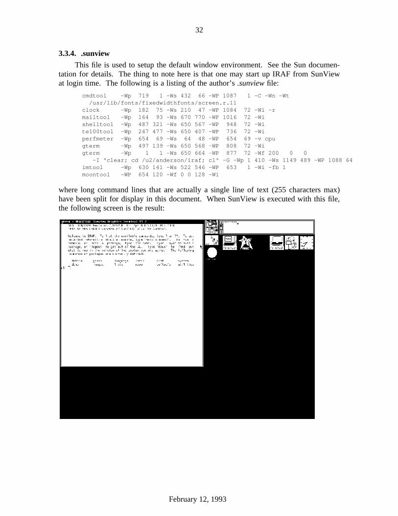
32

3.3.4. .sunview

This file is used to setup the default window environment. See the Sun documen-tation for details. The thing to note here is that one may start up IRAF from SunViewat login time. The following is a listing of the author’s .sunview file:

cmdtool -Wp 719 1 -Ws 432 66 -WP 1087 1 -C -Wn -Wt/usr/lib/fonts/fixedwidthfonts/screen.r.11

clock -Wp 182 75 -Ws 210 47 -WP 1084 72 -Wi -rmailtool -Wp 164 93 -Ws 670 770 -WP 1016 72 -Wishelltool -Wp 487 321 -Ws 650 567 -WP 948 72 -Wite100tool -Wp 247 477 -Ws 650 407 -WP 736 72 -Wiperfmeter -Wp 654 69 -Ws 64 48 -WP 654 69 -v cpugterm -Wp 497 139 -Ws 650 568 -WP 808 72 -Wigterm -Wp 1 1 -Ws 650 664 -WP 877 72 -Wf 200 0 0

-I "clear; cd /u2/anderson/iraf; cl" -G -Wp 1 410 -Ws 1149 489 -WP 1088 64imtool -Wp 630 141 -Ws 522 546 -WP 653 1 -Wi -fb 1moontool -WP 654 120 -Wf 0 0 128 -Wi

where long command lines that are actually a single line of text (255 characters max)have been split for display in this document. When SunView is executed with this file,the following screen is the result:.

February 12, 1993

33

3.4. DECstation Setup

IRAF on the DECstation should be run from an xterm window as opposed to adecterm window. This is because decterm does not support cursor readback, andtherefore IRAF interactive graphics cannot work. The images display tool is SAOIM-AGE and is disussed in §4.2.

The DECstation has it’s own set of startup files that allow the user to specify win-dows, icons and positions for both.

3.4.1. .X11Startup

This file is used to set up the user’s default window environment. See the DECdocumentation for details. Note how the second to last xterm window starts up IRAFby executing a file called .goiraf.

(dxcalendar -bw 50 -iconic -geometry 500x350+50+60 &)(saoimage -imtool -g +10+110 &)(xterm -geom 80x24+10+140 -n "xterm1" -fn courier14 &)(xterm -geom 80x24+20+150 -n "xterm4" -fn courier14 -iconic &)(xterm -geom 80x24+500+200 -n "xterm3" -fn courier14 -iconic &)(xterm -geom 80x24+20+500 -n "xterm2" -fn courier14 -iconic &)(xterm -fg red +ls -geom 80x40+300-0 -fn courier14 -e .goiraf &)(xterm -geom 100x100+0+0 -fn courier24 -n "big" &)

The contents of .goiraf are,

cd /usr/users/anderson/irafcl

3.4.2. .Xdefaults

This file is used to set window defaults in general. See the system documentationfor details.

3.4.3. .login and .cshrc

When logging into the DECstation console, the .login file does not seem to beexecuted (at least not before .X11Startup). Thus path and tty definitions need to be putin the .cshrc file.

However, one must be careful how .cshrc is set up, otherwise interference withnetworking (especially IRAF networking) will result. The following example showshow to check for console login and respond accordingly.

set path = (. /usr/local/bin /usr/ucb /bin /usr/bin /etc /usr/etc)setenv IRAFARCH mipssetenv TERM xtermjhsetenv PRINTER lw7setenv R_DISPOSE "lpr -Plw7 -r %s"setenv iraf /usr/iraf/

# Check for console login.if ("’tty’" == "ttyp0") then

stty new dec cr0 ff0 crt -tabs susp ’^X’ eof ’^Z’endif

February 12, 1993

34

4. Generic Image Processing

This section will discuss how to use the generic image processing, display andplotting tasks of IRAF. There are always a variety of ways to accomplish some imageprocessing task, and therefore the reader must remember that the methodologydescribed in the following subsections is that of the author. This discussion is meant tobe used as a guide to the reduction and analysis of image data in general, and is not acookbook peculiar to some instrument and/or detector combination.

4.1. Getting Data In and Out of IRAF (DATAIO)

At present, there are two basic IRAF file types: imagefiles and textfiles. As notedin the GRASP Database Specifications (November 1988, internal project report), almostall of the GONG data (i.e., images, time series and power spectra) will be stored asIRAF images (i.e., .imh files) when being used from GRASP.

The purpose of the DATAIO package is to provide the tools necessary to convertIRAF files to standard transportable formats and vice-versa. In astronomy, there areonly two machine independent, transportable formats:

ASCII TextAn ASCII text file is a human readable file when printed at the terminal.Indeed, the IRAF text file (as mentioned in §2.13) is an ASCII text file. TheDATAIO routines that are concerned with text files allow one to read/writethese files from/to tape or disk with user specified line lengths, blocksizes,etc., and even EBCDIC encoding if an IBM machine is involved.

FITS ImageThe Flexible Image Transport System was originally developed as a 9-tracktape format for the machine independent transfer of image data. Since itsinception, it has become the most widely used format in astronomy, and ithas been extended to cover more complex data types (e.g., groups and tables).For the purposes of GONG, the basic, standard FITS is all that is required totransport the image data. The DATAIO package provides two routines (rfitsand wfits) that allow one to convert between IRAF and FITS format images(to/from tape or disc).

The following is the help menu for the DATAIO package.

dataio.:bintxt - Convert a binary file to an IRAF text file

mtexamine - Examine the structure of a magnetic tapercardimage - Convert a cardimage file into a text file

reblock - Copy a binary file, optionally reblockingrfits - Convert a FITS image into an IRAF image

rtextimage - Convert text files to IRAF imagest2d - Fast tape to disk copy

txtbin - Convert an IRAF text file to a binary filewcardimage - Convert text files to cardimage files

wfits - Convert an IRAF image into a FITS imagewtextimage - Convert an IRAF image to a text file

February 12, 1993

35

4.1.1. General Tape Handling

4.1.1.1. Device Allocation & Deallocation

Before one may use any of the tape routines, a tape drive must be allocated. AllIRAF tape devices are named mt[abcde...], no matter what the host system happens tocall them. Use the devices command (cf. §2.18.3) to locate the desired tape unit and itscorresponding IRAF device name.

� To allocate a tape unit which belongs to the host system from which you are run-ning the CL, enter a command of the form,

da> allocate device_name

� To allocate a tape unit that belongs to another host on the IRAF network, enter acommand of the form,

da> allocate host_name!device_name

� To deallocate a device, enter a command of the form,

da> deallocate [host_name!]device_name

NOTE: The allocate command is a system package command, and thus the DATAIOpackage does not need to be loaded before one can use this command.

4.1.1.2. Tape Density Specification

When reading tapes, it should not be necessary to inform the system (e.g., IRAF orthe host) of the tape density. However, when writing onto blank tapes, or overwritingused tapes, it is very important to inform IRAF of the desired density. For most sys-tems (e.g., UNIX host environments) this information is passed by the specific taskbeing used by appending the desired density to the device name. For example,

mta6250 # device mta at 6250 bpi

mtb1600 # device mtb at 1600 bpi

VMS USERS NOTE:Since tape allocation at the host level on VMS systems involves both an allo-cate and a mount command (where the mount specifies the tape density), it isnecessary to have blank tapes, or tapes which are to be overwritten at adifferent density, reinitialized to the desired density BEFORE issuing theIRAF allocate command. For example, to write onto a new tape at 6250bpi,the following sequence of commands will guarantee the desired density:

da> # First load the tape on the desired device (say MUA0:)da> !init/den=6250 mua0: tape # Initialize the tapeda> allocate mta # Allocate the tape drive from IRAF

Although the initialize command will label the tape, this label will beoverwritten by whatever IRAF task that is used.

February 12, 1993

36

4.1.1.3. Tape positioning

Tapes never have to be pre-positioned at the beginning of the desired file (i.e., skipforward or skip backward) in order to use any of the IRAF tape handling routines.

� To rewind a tape, enter a command of the form,

da> rewind [host_name!]device_name

� To check the status of a tape (e.g., current position) enter a command of the form,

da> devstatus [host_name!]device_name

For example,

da> devstat gemini!mta# Magtape unit ‘gemini!mta’ allocated to ‘anderson’ Mon 14:07:01 21-May-90file = 50record = 1 (EOT)

indicates that the unit is allocated and positioned at the beginning of file 50, whichalso happens to be the logical end-of-tape (EOT).

Note that devstatus is a useful command for finding out who has what devicesallocated. For example,

da> devstat orion!mtadevice orion!mta is not currently allocatedda>da> devstat orion!mtbdevice orion!mtb currently allocated to pintar

� The tape readers have a string parameter called file_list that is used to specifywhich files on the tape are to be read. The string can consist of any sequence offile numbers separated by commas, or dashes. A dash specifies a range of files.For example the string

"1,3,13-15,18-26"

specifies the files 1, 3, 13 through 15 and 18 through 26. To read the whole tape,one need give only a suitably large range (e.g., "1-999").

� The tape writers have a boolean parameter called new_tape which, if no specifictape file number is given in the output device name, will automatically start writ-ing at the logical EOT (i.e., double EOF).

Should the user wish to overwrite data, starting at some particular file number,then that place is specified with the output device name. For example:

mta6250[100]

will tell the task to start writing at file 100.

February 12, 1993

37

4.1.2. Textfile I/O

The tasks [rw]cardimage are usually used to read (or write) cardimage tapes, con-verting the tapefiles to IRAF text files. These routines will also work on disk files. Thefollowing are a few brief examples of the use of each of these tasks:

da> lpar rcardimagecardfile = Card image filefile_list = List of tape file numberstextfile = Output file text file(s)

join = no Join oversize lines?contn_string = ">>" Continuation line marker

(mode = "ql")(card_length = 80) Columns per card(max_line_len = 161) Maximum line length

(entab = yes) Replace blanks with tabs and blanks?(trim = yes) Trim trailing whitespace?

(verbose = yes) Print messages?(ebcdic = no) Convert from EBCDIC to ASCII?

(ibm = no) Translate from IBM(EBCDIC) to ASCII?(offset = 0) Tape file number offset

Example 4.1.1:To read all the files from a standard cardimage tape (e.g., 80 columns per card,and say 50 cards per block), not replacing blanks with tabs and blanks, and trim-ming trailing whitespace from each line, use a command of the form,

da> rcard mta 1-999 card j- entab-

The output text files would be called card001, card002, ... (i.e., the tape filenumber is concatenated to the root output file name).

Example 4.1.2:Assume that one now wishes to read in a second tape and have the numbering ofthe output files continue from where the first tape left off (for the sake of example,let’s say that 100 files were read from the first tape). For this, one uses the offsetparameter:

da> rcard mta 1-999 card j- entab- offset=100

The file names from this read will be "card"//100+tape_file_number (i.e., card101,card102, ...).

Example 4.1.3:There is a hidden parameter called max_line_length which defaults to 161 charac-ters per output line (the maximum size permitted by IRAF). This parameter isuseful for stripping the documentation characters from Fortran programs (i.e.,columns 73-80).

da> rcard mta 1 program.f j- entab- max_line=72

February 12, 1993

38

da> lpar wcardimagetextfile = Text file(s)cardfile = Card image file(s)new_tape = Blank tape?

(mode = "ql")(contn_string = ">>") Marker for oversize lines

(verbose = yes) Print messages of actions performed?(detab = yes) Detab string and replace with blanks?

(card_length = 80) Columns per card(cards_per_bl = 50) Card images per block

(ebcdic = no) Convert from ASCII to EBCDIC?(ibm = no) Convert from ASCII to IBM(EBCDIC)?

Example 4.1.4:To write several files (say a fortran program and data files) to tape at 1600bpi, 80columns per card and 50 cards per block (i.e., blocksize 4000 default), starting atthe beginning of the tape, a command of the following form would be used:

da> wcard prog.f,data* mtb1600 new+

Example 4.1.5:Suppose that the data file lines were 132 characters wide, but to ensure transport toa different machine, you wanted to limit the line length to 80 characters. Theabove command would make use of the parameter contn_string which breaks uplong data records into several records appending the specified character(s) (default">>") to indicate that the following card needs to be concatenated to the presentcard when the file is to be reconstructed. RCARDIMAGE also has the sameparameter, and an additional boolean parameter, join, with which the user mayspecify whether or not the records are to be concatenated.

Thus to restore the files from the above example, one would use commands of thefollowing form:

da> rcard mta 1 prog.fda> rcard mta 2-999 data join+ offset=-1

Where the use of the offset parameter is to ensure that the data files would benamed data001, data002, ....

Example 4.1.6:Suppose that you want the long data records written on one card, then a commandof the following form would be necessary.

da> wcard prog.f,data* mta1600 new+ card_len=132

Note, that the blocksize of this tape is 6600 (132 × 50).

February 12, 1993

39

The tasks [rw]textimage are used to convert between IRAF text files and images.Generally the text file is just a list of numbers (i.e., array elements) that are assembledinto n-dimensional images.† Both of these tasks have options for reading/creatingpsuedo-FITS headers at the beginning of the file.

da> lpar rtextimageinput = "" Input text fileoutput = "" Output image file(otype = "") Pixel type on output(header = yes) Read FITS header preceding pixels?(nskip = 0) Number of lines to skip

(dim = ) Image dimension string(mode = "ql")

Example 4.1.7:Consider a text file (called say pix1.txt) that is a list of integers representing a512x512 image.

da> head pix1.txt38 43 35 43 39 39 41 41 41 37 3737 37 37 39 36 43 41 38 34 33 3739 40 41 44 36 36 42 36 36 41 3941 41 38 41 41 37 39 46 45 41 38

To convert this file into an image, the command:

da> rtext pix1.txt pix1 ot=r h- dim=512,512

will create an image, pix1.imh, of pixel type real (ot=r). The parameter h-informs the task that no header information (i.e., leading text) is present.

Example 4.1.8:To read a data file skipping some sort of text information at the beginning of thatfile, one uses the nskip parameter to skip over the specified number of lines in thefile before attempting to convert data into the image. For example,

da> head pix1.txtMay 13, 1990Program myprogramInput myinputblah blah

38 43 35 43 39 39 41 41 41 37 3737 37 37 39 36 43 41 38 34 33 3739 40 41 44 36 36 42 36 36 41 3941 41 38 41 41 37 39 46 45 41 38

da>da> rtext pix1.txt pix1 ot=r h- dim=512,512 nskip=4

Should one need to transport images to a machine which does not have IRAF or aFITS reader, then one will need to convert the image to a text file using wtextimage.One may create a pixel data only file, or you may create a file which has a pseudo-FITSheader containing the relevant information about array dimensions, and also all other

† Remember that the arrays are read/written with the left-most subscript changing most rapidly(i.e., [1,1,1], [2,1,1], [3,1,1], ...).

February 12, 1993

40

IRAF image header information.

da> lpar wtextimageinput = "" Input image file

output = "" Output text file(header = yes) Print header information?(format = "") Pixel format <w.d[defgz]>

(maxlinelen = 80) Maximum line length output(mode = "ql")

Example 4.1.9:To create a pixel data only text file from the IRAF test image, dev$pix.

da> wtext dev$pix pix.txt h-da> head pix.txt

38 43 35 43 39 39 41 41 41 37 3737 37 37 39 36 43 41 38 34 33 3739 40 41 44 36 36 42 36 36 41 3941 41 38 41 41 37 39 46 45 41 38

Example 4.1.10:The following creates a text file with the pseudo-FITS header:

da> wtext dev$pix pix.txtda> head pix.txtBITPIX = 8 / 8-bit ASCII charactersNAXIS = 2 / Number of Image DimensionsNAXIS1 = 512 / Length of axisNAXIS2 = 512 / Length of axisORIGIN = ’NOAO-IRAF: WTEXTIMAGE’ /IRAF-MAX= 19936. / Max image pixelIRAF-MIN= -1. / Min image pixelIRAF-B/P= 16 / Image bits per pixelIRAFTYPE= ’SHORT INTEGER ’ / Image datatypeOBJECT = ’M51 B 600S ’ /FILENAME= ’DEV$PIX ’ / IRAF filenameFORMAT = ’11I7 ’ / Text line format

Creating the text image in this way ensures that no image header information willbe lost enroute to the destination machine.

Example 4.1.11:To read a file with header information, the following keywords must be included:NAXIS, NAXIS1, etc. To create an IRAF image of datatype real from the textimage of the above example, the command would be,

da> rtext pix.txt m51_blue ot=r

Example 4.1.12:As a final example, the following command combines rcardimage and rtextimagein a pipe to read a text file with a non-FITS header of 5 cards and create a256x512 image of type real.

da> rcard mta[1] j- entab- | rtext mydata h- dim=256,512 ot=r, nskip=5

February 12, 1993

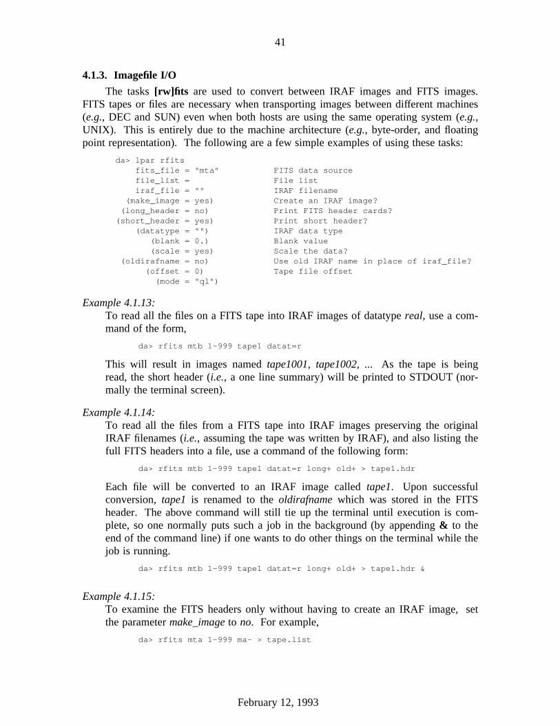
41

4.1.3. Imagefile I/O

The tasks [rw]fits are used to convert between IRAF images and FITS images.FITS tapes or files are necessary when transporting images between different machines(e.g., DEC and SUN) even when both hosts are using the same operating system (e.g.,UNIX). This is entirely due to the machine architecture (e.g., byte-order, and floatingpoint representation). The following are a few simple examples of using these tasks:

da> lpar rfitsfits_file = "mta" FITS data sourcefile_list = File listiraf_file = "" IRAF filename

(make_image = yes) Create an IRAF image?(long_header = no) Print FITS header cards?

(short_header = yes) Print short header?(datatype = "") IRAF data type

(blank = 0.) Blank value(scale = yes) Scale the data?

(oldirafname = no) Use old IRAF name in place of iraf_file?(offset = 0) Tape file offset(mode = "ql")

Example 4.1.13:To read all the files on a FITS tape into IRAF images of datatype real, use a com-mand of the form,

da> rfits mtb 1-999 tape1 datat=r

This will result in images named tape1001, tape1002, ... As the tape is beingread, the short header (i.e., a one line summary) will be printed to STDOUT (nor-mally the terminal screen).

Example 4.1.14:To read all the files from a FITS tape into IRAF images preserving the originalIRAF filenames (i.e., assuming the tape was written by IRAF), and also listing thefull FITS headers into a file, use a command of the following form:

da> rfits mtb 1-999 tape1 datat=r long+ old+ > tape1.hdr

Each file will be converted to an IRAF image called tape1. Upon successfulconversion, tape1 is renamed to the oldirafname which was stored in the FITSheader. The above command will still tie up the terminal until execution is com-plete, so one normally puts such a job in the background (by appending & to theend of the command line) if one wants to do other things on the terminal while thejob is running.

da> rfits mtb 1-999 tape1 datat=r long+ old+ > tape1.hdr &

Example 4.1.15:To examine the FITS headers only without having to create an IRAF image, setthe parameter make_image to no. For example,

da> rfits mta 1-999 ma- > tape.list

February 12, 1993

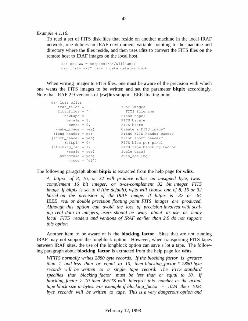
42

Example 4.1.16:To read a set of FITS disk files that reside on another machine in the local IRAFnetwork, one defines an IRAF environment variable pointing to the machine anddirectory where the files reside, and then uses rfits to convert the FITS files on theremote host to IRAF images on the local host.

da> set ww = serpens!/d4/williams/da> rfits ww$*.fits 1 data datat=r old+

When writing images to FITS files, one must be aware of the precision with whichone wants the FITS images to be written and set the parameter bitpix accordingly.Note that IRAF 2.9 versions of [rw]fits support IEEE floating point.

da> lpar wfitsiraf_files = IRAF imagesfits_files = "" FITS filename

newtape = Blank tape?bscale = 1. FITS bscalebzero = 0. FITS bzero

(make_image = yes) Create a FITS image?(long_header = no) Print FITS header cards?

(short_header = yes) Print short header?(bitpix = 0) FITS bits per pixel

(blocking_fac = 1) FITS tape blocking factor(scale = yes) Scale data?

(autoscale = yes) Auto_scaling?(mode = "ql")

The following paragraph about bitpix is extracted from the help page for wfits.

A bitpix of 8, 16, or 32 will produce either an unsigned byte, twos-complement 16 bit integer, or twos-complement 32 bit integer FITSimage. If bitpix is set to 0 (the default), wfits will choose one of 8, 16 or 32based on the precision of the IRAF image. If bitpix is -32 or -64IEEE real or double precision floating point FITS images are produced.Although this option can avoid the loss of precision involved with scal-ing real data to integers, users should be wary about its use as manylocal FITS readers and versions of IRAF earlier than 2.9 do not supportthis option.

Another item to be aware of is the blocking_factor. Sites that are not runningIRAF may not support the longblock option. However, when transporting FITS tapesbetween IRAF sites, the use of the longblock option can save a lot a tape. The follow-ing paragraph about blocking_factor is extracted from the help page for wfits.

WFITS normally writes 2880 byte records. If the blocking factor is greaterthan 1 and less than or equal to 10, then blocking_factor * 2880 byterecords will be written to a single tape record. The FITS standardspecifies that blocking_factor must be less than or equal to 10. Ifblocking_factor > 10 then WFITS will interpret this number as the actualtape block size in bytes. For example if blocking_factor = 1024 then 1024byte records will be written to tape. This is a very dangerous option and

February 12, 1993

43

has been included to accommodate users with restricted block size devicessuch as SUN microcassettes. WFITS will issue a warning message if it seesan illegal block size before it begins to execute.

Example 4.1.17:To write an autoscaled FITS tape with files packed at the largest standard blockingand with 32 bit precision, one would use a command of the following form:

da> wfits vmi*.imh mtb6250 new+ bit=32 block=10

Example 4.1.18:To write a standard 2880 blocksize FITS tape from a list of images in a textfilecalled tapein, forcing 16 bit precision, listing the short header to the default printerand appending to the end of a tape, one would use a command of the form,

da> wfits @tapein mtb6250 new- bit=16 | lprint

NOTE: Care must be taken when FITSing 3-d (or higher dimension) images when thebands contain different types of data (i.e., greatly different means anddynamic ranges, for example GONG vmi images) as autoscaling will be basedon the dynamic range of the combined bands and might destroy all the data ina given band. It may be necessary to separate the bands into individualimages before writing the tape.

4.1.4. Dealing With Unknown Tapes

The most common cause of tape read frustration (at least according to theauthor’s experience) is insufficient information about the tape being passed along withthe tape. All tapes, whether 9-track, cartridge or 8mm cassettes must be properlylabelled for the convenience of the user. The label should contain the owner’s name,date written, tape format, tape density, and depending on the format, maximum recordand block sizes. For example,

Ed Anderson 20Jan909 tr

Power Spectra 6250 bpi(June 8, 89) FITS

Ed Anderson 20Feb909 tr

GRASP 6250 bpiblocksize=126 TAR

February 12, 1993

44

Ed Anderson 20Feb909 tr

Gapfill Source 1600 bpiCardimage blocksize=4000EBCDIC recordsize=80

The tasks mtexamine, reblock, and t2d are useful for attempting to identify thecontents of unknown tapes and manipulate the contents into something that can be used.

The task mtexamine allows one to examine the file structure on the tape (or evena diskfile). The user may selectively dump records in various formats in order to helpestablish the file structure.

da> lpar mtexaminetape_file = "mtb" Tape file(file_list = "1-999") List of file numbers

(dump_records = no) Dump selected records?(rec_list = "1-999") List of records to be dumped

(byte_chunk = 1) Byte chunk(swapbytes = no) Swap bytes?

(output_forma = "o") Dump format (c|d|o|u|x)(mode = "ql")

Example 4.1.19:To list the overall structure of a tape, run mtexamine with all its defaults. Forexample,

da> mtex mtaFile mta[1]:

476 4000-byte records1 2560-byte recordsTotal 477 records, 1906560 bytes

File mta[2]:478 4000-byte records1 160-byte recordsTotal 479 records, 1912160 bytes

File mta[3]:953 2000-byte records1 520-byte recordsTotal 954 records, 1906520 bytes

File mta[4]:Total 0 records, 0 bytes

Tape at EOT

These results suggest that the files are cardimage text files. This can be confirmed,by doing a character dump of the first block of file 1.

da> mtex mta file=1 dump+ rec=1 output=c | pageFile mta[1]:

Record 1, 4000 bytes, 4000 elements1: 3 8 4 3

16: 3 5 4 331: 3 9 3 946: 4 1 4 1

February 12, 1993

45

61: 4 1 3 776: 3 7 3 791: 3 7 3 7106: 3 9 3 6121: 4 3 4 1 3136: 8 3 4 3 3151: 3 7166: 3 9 4 0 4

This dump would seem to confirm that the file is ASCII text. The fact that theblocksize is 4000 (i.e., a multiple of 80) would lead one to attempt to read the tapeat a recordsize of 80.

NOTE: Reported blocksizes of 2880 or some multiple (up to 10) usually imply thatthe tape is a FITS tape.

Blocksizes evenly divisible by 80 or 132 usually imply a cardimage tape.

The task reblock allows the user to restructure a tape (or diskfile) by copying to anew tape (or diskfile) with optional reblock, byte-swapping, word-swapping, blockand/or record padding.

tv> lpar reblockinfiles = Input file

outfiles = Output filefile_list = Tape file list

newtape = Blank tape?(outblock = INDEF) Size of output block in bytes(inrecord = INDEF) Size of input records in bytes(outrecord = INDEF) Size of output records in bytes(pad_block = no) Pad last block?

(padchar = "0") Pad character(skipn = 0) Skip n blocks (tape) or records (disk)(copyn = INDEF) Copy n blocks (tape) or records (disk)

(byteswap = no) Swap bytes?(wordswap = no) Swap words?

(offset = 0) Tape file number offset(verbose = yes) Print messages?

(mode = "ql")

Example 4.1.20:A common error made by many sites when writing FITS tapes is to have the byteorder incorrect. That is, the byte order seems fine for their site, but is byte-swapped to the standard. More often than not, the FITS header is byte-swappedalso, and rfits will complain. The following is a dump of the first few lines of anincorrect (i.e, byte-swapped) FITS header:

ISPMEL = T /F TI STSNAADDRIBPTXI = 61 /F TI SIBSTP/XILEANIX S = 2 /N MUEB RFOA EX SANIX1S = 5 21 /ANIX2S = 5 21 /SBACEL = .100000000000E /R AE L =ATEPB*CSLA E +ZBRE OZBRE O = .000000000000E /BOEJTC =m’15 B6 00’s /

February 12, 1993

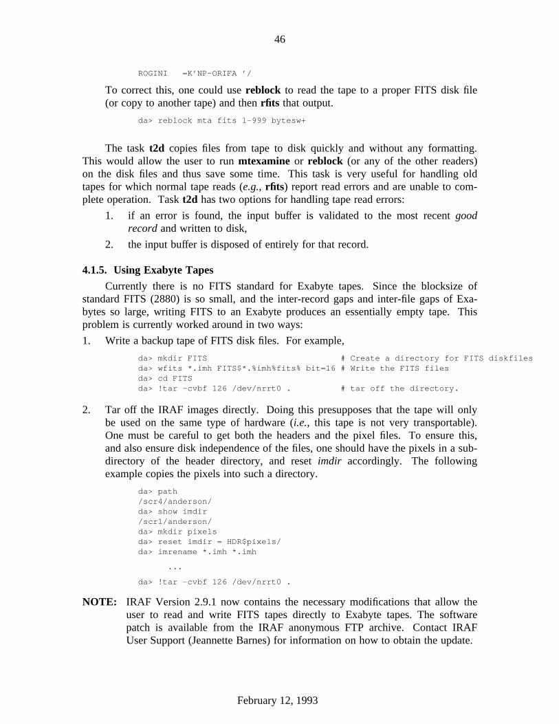
46

ROGINI =K’NP-ORIFA ’/

To correct this, one could use reblock to read the tape to a proper FITS disk file(or copy to another tape) and then rfits that output.

da> reblock mta fits 1-999 bytesw+

The task t2d copies files from tape to disk quickly and without any formatting.This would allow the user to run mtexamine or reblock (or any of the other readers)on the disk files and thus save some time. This task is very useful for handling oldtapes for which normal tape reads (e.g., rfits) report read errors and are unable to com-plete operation. Task t2d has two options for handling tape read errors:

1. if an error is found, the input buffer is validated to the most recent goodrecord and written to disk,

2. the input buffer is disposed of entirely for that record.

4.1.5. Using Exabyte Tapes

Currently there is no FITS standard for Exabyte tapes. Since the blocksize ofstandard FITS (2880) is so small, and the inter-record gaps and inter-file gaps of Exa-bytes so large, writing FITS to an Exabyte produces an essentially empty tape. Thisproblem is currently worked around in two ways:

1. Write a backup tape of FITS disk files. For example,

da> mkdir FITS # Create a directory for FITS diskfilesda> wfits *.imh FITS$*.%imh%fits% bit=16 # Write the FITS filesda> cd FITSda> !tar -cvbf 126 /dev/nrrt0 . # tar off the directory.

2. Tar off the IRAF images directly. Doing this presupposes that the tape will onlybe used on the same type of hardware (i.e., this tape is not very transportable).One must be careful to get both the headers and the pixel files. To ensure this,and also ensure disk independence of the files, one should have the pixels in a sub-directory of the header directory, and reset imdir accordingly. The followingexample copies the pixels into such a directory.

da> path/scr4/anderson/da> show imdir/scr1/anderson/da> mkdir pixelsda> reset imdir = HDR$pixels/da> imrename *.imh *.imh

...

da> !tar -cvbf 126 /dev/nrrt0 .

NOTE: IRAF Version 2.9.1 now contains the necessary modifications that allow theuser to read and write FITS tapes directly to Exabyte tapes. The softwarepatch is available from the IRAF anonymous FTP archive. Contact IRAFUser Support (Jeannette Barnes) for information on how to obtain the update.

February 12, 1993

47

4.2. Image Display (TV)

The TV package contains the tasks necessary to display images on various dev-ices. This package is currently undergoing major revision and therefore contains manytasks which may not be needed depending on the image display device being used. Thefollowing is the help menu for the TV package:

tv.:blink - Blink two frames

cv - Control image device, display "snapshot"cvl - Load image display (newer version of ’display’)

display - Load an image or image section into the displayerase - Erase an image frameframe - Select the frame to be displayed

lumatch - Match the lookup tables of two framesmonochrome - Select monochrome enhancement

pseudocolor - Select pseudocolor enhancementrgb - Select true color mode (red, green, and blue frames)

window - Adjust the contrast and dc offset of the current framezoom - Zoom in on the image (change magnification)

These tasks comprise three levels of image display software.

1.) The task display is used to load an image into any display device supportedby IRAF, including workstation windows (i.e., IMTOOL or SAOIMAGE).

2.) The Captain Video routines are used for video display devices such as I 2S.The tasks cvl (Captain Video Load) and cv (Captain Video) are used to loadand play with images respectively.

3.) All other tasks are obsolete video display tasks (some of which may onlywork on an I 2S). All of these functions and more are available withinIMTOOL, SAOIMAGE and cv.

NOTE: The workstation display windows (IMTOOL for Sun, and SAOIMAGE forDEC) are not yet capable of real color image display via rgb frame overlaysas they use only 8-bit frame buffers.

The following sections present a summary description of how to use the TV pack-age and display windows. The user is strongly encouraged to read the help pages forthe appropriate task and/or window as the following is by no means an exhaustive treat-ment of the subjects.

4.2.1. TV.DISPLAY

The task display is used to load IRAF images into any supported display device.The device (or display window) to be used is set via the IRAF environment variablestdimage. The following is the parameter listing for display:

tv> lpar displayimage = "q" image to be displayedframe = 1 frame to be written into(erase = yes) erase frame

(border_erase = no) erase unfilled area of window

February 12, 1993

48

(select_frame = yes) display frame being loaded(repeat = no) repeat previous display parameters

(fill = no) scale image to fit display window(zscale = yes) display range of greylevels near median

(contrast = 0.25) contrast adjustment for zscale algorithm(zrange = yes) display full image intensity range

(nsample_line = 5) number of sample lines(xcenter = 0.5) display window horizontal center(ycenter = 0.5) display window vertical center(xsize = 1.) display window horizontal size(ysize = 1.) display window vertical size(xmag = 1.) display window horizontal magnification(ymag = 1.) display window vertical magnification(order = 0) spatial interpolator order (0=replicate,1=linear)

(z1 = ) minimum greylevel to be displayed(z2 = ) maximum greylevel to be displayed

(ztrans = "linear") greylevel transformation (linear|log|none)(lutfile = "") file containing user defined look up table

(mode = "ql")

Although there are lots of parameters, the task only needs to know the image nameand the frame number into which the image should be displayed. For workstationdisplay windows, the number of frames can be set by the user for various window sizes(note that these frames cannot be overlayed). The other parameters can be lumped intoseveral groups:

erase, border_eraseIf erase = yes, the contents of the frame are erased before displaying the newimage.

If erase = no and border_erase = yes, the new image is displayed first andthen that part of the visible display frame not taken up by the new image iserased. This is only useful for workstation windows where the visibledisplay frame may be smaller than the frame buffer and hence usingborder_erase will result in a faster display execution.

Using erase = no allows one to display several images in one frame (i.e.,display mosaicing).

select_frameIf select_frame = no, then display will load the desired frame without switch-ing the image display to that frame first.

This is useful for demonstrations, etc., when one is using multiple frames andcan be looking at one frame while loading another.

repeatNot yet implemented.

fill, xmag, ymag, orderThese parameters control the size or magnification of the image in the displayframe.

February 12, 1993

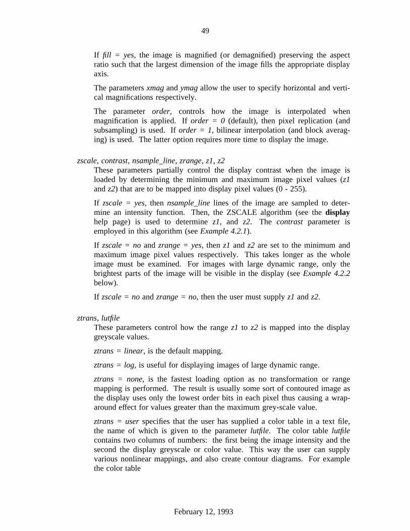
49

If fill = yes, the image is magnified (or demagnified) preserving the aspectratio such that the largest dimension of the image fills the appropriate displayaxis.

The parameters xmag and ymag allow the user to specify horizontal and verti-cal magnifications respectively.

The parameter order, controls how the image is interpolated whenmagnification is applied. If order = 0 (default), then pixel replication (andsubsampling) is used. If order = 1, bilinear interpolation (and block averag-ing) is used. The latter option requires more time to display the image.

zscale, contrast, nsample_line, zrange, z1, z2These parameters partially control the display contrast when the image isloaded by determining the minimum and maximum image pixel values (z1and z2) that are to be mapped into display pixel values (0 - 255).

If zscale = yes, then nsample_line lines of the image are sampled to deter-mine an intensity function. Then, the ZSCALE algorithm (see the displayhelp page) is used to determine z1, and z2. The contrast parameter isemployed in this algorithm (see Example 4.2.1).

If zscale = no and zrange = yes, then z1 and z2 are set to the minimum andmaximum image pixel values respectively. This takes longer as the wholeimage must be examined. For images with large dynamic range, only thebrightest parts of the image will be visible in the display (see Example 4.2.2below).

If zscale = no and zrange = no, then the user must supply z1 and z2.

ztrans, lutfileThese parameters control how the range z1 to z2 is mapped into the displaygreyscale values.

ztrans = linear, is the default mapping.

ztrans = log, is useful for displaying images of large dynamic range.

ztrans = none, is the fastest loading option as no transformation or rangemapping is performed. The result is usually some sort of contoured image asthe display uses only the lowest order bits in each pixel thus causing a wrap-around effect for values greater than the maximum grey-scale value.

ztrans = user specifies that the user has supplied a color table in a text file,the name of which is given to the parameter lutfile. The color table lutfilecontains two columns of numbers: the first being the image intensity and thesecond the display greyscale or color value. This way the user can supplyvarious nonlinear mappings, and also create contour diagrams. For examplethe color table

February 12, 1993

50

0 060 20060.01 0100 200100.01 0200 200200.01 0300 200300.01 0400 200400.01 0420 200

was used to produce the contoured image of Example 4.2.4 below.

xcenter, ycenter, xsize, ysizeThese parameters control the positioning of the image in the display windowwhich is defined in term of the full frame (i.e., (0,0) is the lower left cornerand (1,1) is the upper right corner).

xcenter and ycenter set the position of the center of the image to be displayedand may range from 0 to 1.

xsize and ysize set the fraction of the display window that may be used for agiven image.

These four parameters are very useful when mosaicing images (especially ofdifferent sizes) into one display frame (see Example 4.2.5 below).

February 12, 1993

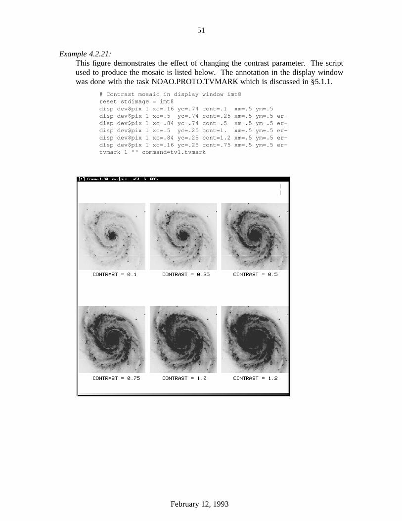
51

Example 4.2.21:This figure demonstrates the effect of changing the contrast parameter. The scriptused to produce the mosaic is listed below. The annotation in the display windowwas done with the task NOAO.PROTO.TVMARK which is discussed in §5.1.1.

# Contrast mosaic in display window imt8reset stdimage = imt8disp dev$pix 1 xc=.16 yc=.74 cont=.1 xm=.5 ym=.5disp dev$pix 1 xc=.5 yc=.74 cont=.25 xm=.5 ym=.5 er-disp dev$pix 1 xc=.84 yc=.74 cont=.5 xm=.5 ym=.5 er-disp dev$pix 1 xc=.5 yc=.25 cont=1. xm=.5 ym=.5 er-disp dev$pix 1 xc=.84 yc=.25 cont=1.2 xm=.5 ym=.5 er-disp dev$pix 1 xc=.16 yc=.25 cont=.75 xm=.5 ym=.5 er-tvmark 1 "" command=tv1.tvmark

.

February 12, 1993

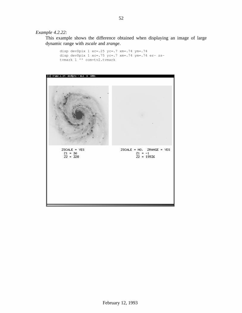
52

Example 4.2.22:This example shows the difference obtained when displaying an image of largedynamic range with zscale and zrange.

disp dev$pix 1 xc=.25 yc=.7 xm=.74 ym=.74disp dev$pix 1 xc=.75 yc=.7 xm=.74 ym=.74 er- zs-tvmark 1 "" com=tv2.tvmark

.

February 12, 1993

53

Example 4.2.23:This example shows the differences in the three ztrans functions.

disp dev$pix 1 xc=.17 yc=.7 xm=.5 ym=.5disp dev$pix 1 xc=.5 yc=.7 xm=.5 ym=.5 zt="log" er-disp dev$pix 1 xc=.83 yc=.7 xm=.5 ym=.5 zt="none" er-tvmark 1 "" com=fig3.tvmark

.

February 12, 1993

54

Example 4.2.24:This example shows how a user provided color table can be used to create con-toured images. The image on the left is the default display. The image on theright is displayed with the color table shown below.

tv> type color.tab0 0

60 20060.01 0100 200100.01 0200 200200.01 0300 200300.01 0400 200400.01 0420 200

tv> disp radial 1 xc=.25 yc=.7 xm=.74 ym=.74tv> disp radial 1 xc=.75 yc=.7 xm=.74 ym=.74 ztran=user lutfil=color.tab er-

.

February 12, 1993

55

Example 4.2.25:This example demonstrates the mosaicing of images of different sizes into onewindow, filling the available space. Note how xsize and ysize are used to enforcea gap between the various images.

tv> imhead dev$pix,tardis,reflect,balls3dev$pix[512,512][short]: m51 B 600stardis[72,117][short]:reflect[482,691][short]:balls3[880,880][short]:tv> disp dev$pix 1 xc=.25 yc=.75 xs=.49 ys=.49 fill+tv> disp tardis 1 xc=.75 yc=.75 xs=.49 ys=.49 fill+ er-tv> disp reflect 1 xc=.25 yc=.25 xs=.49 ys=.49 fill+ er-tv> disp balls3 1 xc=.75 yc=.25 xs=.49 ys=.49 fill+ er-

.

February 12, 1993

56

4.2.2. IMTOOL

IMTOOL is the image display server for the SunView environment. The serverconsists of a set of N (1≤N≤4) frame buffers and a single display window. The framebuffers are currently 8 bits deep and the number and size is user configurable.

The display window looks at all or a portion of the frame buffer, and its size maybe changed at any time without affecting the contents of the frame buffer(s). The posi-tion of a small window on a large frame buffer may be changed at any time by panningthe window across the buffer.

NOTE: While multiple buffers are available, only one IMTOOL window may be usedat any one time.

There are many menu selections, buttons, and function keys as well as the mousebuttons that affect IMTOOL. The following subsections are taken almost directly fromthe manual pages for IMTOOL, with some of the more detailed explanations edited out.

4.2.2.1. Frame Buffer Configuration

Currently, it is necessary to define the possible frame buffer configurations atstartup time. This is done via a table file called the imtoolrc file. This file normallyresides in /local/lib, but individual users may define their own file (e.g., .imtoolrc)which contains special configurations for their own use. An example illustrating thecontents of such a file is shown below. Note that this may differ from the defaultconfiguration file used at your site.

1 2 512 512 # imt1|imt5122 2 800 800 # imt2|imt8003 2 1024 1024 # imt3|imt10244 1 1600 1600 # imt4|imt16005 1 2048 2048 # imt5|imt20486 1 4096 4096 # imt6|imt40967 1 4096 1024 # imt7|imt4x18 1 1024 4096 # imt8|imt1x49 2 1144 880 # imt9|imtfs full screen (1152x900 minus frame)

10 2 1144 764 # imt10|imtfs35 full screen at 35mm film aspect ratio11 2 128 128 # imt11|imt12812 2 256 256 # imt12|imt256

20 2 388 576 # imt20|imtgec GEC CCD detector format21 1 3040 976 # imt21|imtkpca KPCA detector format (also 2D-Frutti)22 1 128 1520 # imt22|imt2df1 2D-Frutti23 1 256 1520 # imt23|imt2df2 2D-Frutti24 1 512 1520 # imt24|imt2df5 2D-Frutti25 1 960 1520 # imt25|imt2df9 2D-Frutti26 1 512 800 # imt26|imtcryo Cryogenic Camera27 1 348 800 # imt27|imtgcam Gold Camera28 1 976 3040 # imt28|imt2df9x3 2D-Frutti

30 1 256 800 # imt30|imtgong Gong Cache Monitor

Each entry in the file contains four numbers, the configuration number, the numberof frames to be created initially (frames may be added or deleted once the configurationis specified), and the width and height of the frame in screen pixels. Blank lines andcomments are ignored. Note that the frame width must be evenly divisible by 4, due to

February 12, 1993

57

alignment restrictions on pixel memory in SunView.

Notice in the above example the entry for the Gong Cache Monitor (imt30). Thisis a 256×800 window which allows the simultaneous display of each of the three256×252 planes of the intensity image cube in different portions of the window. Inaddition to adding the new configuration to the imtoolrc file, the IRAF graphcap filemust also be edited (again users may have their own graphcap file). Just copy an entryfor another configuration and then change the window sizes. The following is the entryfor imt30:

imt30|imtgong|GONG Cache Monitor:cn#30:xr#256:yr#800:\:LC:BS@:z0#1:zr#200:DD=node!imtool,/dev/imt1,256,800:tc=iism70:

NOTE: Should a user have a personal imtoolrc file, then the path to that file must bedefined with the UNIX environment variable, IMTOOLRC, in the user’s.login. For example,

setenv IMTOOLRC /u2/anderson/.imtoolrc

4.2.2.2. Executing IMTOOL

There are three preferred ways to create an IMTOOL window of a givenconfiguration.

1.) On most systems IMTOOL is a menu item of the SunView Shell menu (i.e.,the rootmenu). Usually the configuration is imt512.

2.) Users may have their own .rootmenu file in which the IMTOOL configurationcan then be specified with a command of the form,

imtool -fbconfig N

where N is the configuration number in the imtoolrc file.

3.) An IMTOOL window of some desired configuration may be started uponentry into SunView by putting the appropriate command in the .sunview file.For example, the following command creates an imt512 IMTOOL windowconfiguration:

imtool -Wp 630 141 -Ws 522 546 -WP 653 1 -Wi -fb 1

To change the IMTOOL window configuration while running IRAF, change theIRAF environment variable stdimage to the desired configuration. For example,

reset stdimage = imt800

The number of frame buffers can be changed from the IMTOOL setup menu.Configuration changes do not take effect until the next display command is executed.If a smaller sized window is required, the IMTOOL window will automatically changesize on the next display. If a larger configuration is asked for, it is necessary to clickon the fitframe menu selection or setup button during or after the next display shouldviewing of the whole window be desired.

February 12, 1993

58

4.2.2.3. The Frame Menu

The IMTOOL frame menu provides the following selections:

Frame Displays the standard SunView frame menu.

Setup Displays (or hides) the IMTOOL interactive setup panel.

Register Adjusts the pan offset of all frame buffers to match that of theimage currently being displayed. Normally, the individualframe buffers are independently panned.

Blink [on|off] Turns frame blink (alternate display of a series of frames) on oroff. Alternatively the ctrl/B key may be used to manually cyclethrough the blink frames.

FitFrame Adjusts the size of the display window to display the entireframe buffer.

NextFrame Displays the next frame buffer in sequence. Used to cyclethrough and alternately display all frames (the alternate orctrl/F and ctrl/R keys may also be used to cycle forward orreverse through the frames).

Gclear Clear the graphics overlay of the frame currently beingdisplayed.

Iclear Clear the image, (i.e., frame buffer), currently being displayed.

Imcopy Make a hardcopy of the image window.

4.2.2.4. The Setup Panel

The setup panel is used to interactively modify IMTOOL options. Two types ofselections are provided: multiple choice selections, and push button selections. Clickingon a multiple choice selection cycles through the choices (left mouse button) ordisplays the choices as a menu (right mouse button). String valued options aremodified by clicking on the old value, rubbing out all or part of the old value if neces-sary, and then typing in a new value followed by RETURN . If there are several stringvalued fields in a panel, RETURN may be used to cycle through the fields. Clickingon a push button (use the left mouse button) "pushes" the button, causing the actionindicated on the button to be executed.

The multiple choice options in the setup panel are

Number of frame buffersSpecifies the number of frame buffers for which space iscurrently allocated.

Greyscale mappingSpecifies the method to be used to map pixel intensity values toRGB color intensity values.mono specifies that the image is to be rendered in shades ofgrey.linear pseudocolor specifies that the image is to be rendered inpseudocolor, with pixel intensities mapped into the range ofcolors from black to blue to green to red to white.

February 12, 1993

59

random pseudocolor assigns a random color to each possiblepixel greylevel.continuous random pseudocolor is like random pseudocolor, butthe colors are changed every few seconds, where the intervalbetween color changes is specified by the rate option below.

Rate (sec) for Crandom OptionSpecifies the frequency (1 to 32 seconds) with which new colorsare to be assigned for the continuous random pseudocoloroption.

Background colorSpecifies the frame background color of black or white (i.e., thecolor of the portion of the frame buffer which has not been writ-ten into).

Include Frame Border in ImcopySpecifies whether the frame border, including the frame label, isto be included in image hardcopies.

Show colorbarSpecifies whether or not a color bar is to be shown at the bot-tom of the display window.

Blink rate (sec)When blink is enabled, specifies the amount of time a singleframe is to be displayed. The value may range from 1/2 secondto 32 seconds. The maximum blink interval may be achievedby holding down the alternate key long enough to causeautorepeat.

Frames to be blinkedThe string value of this parameter specifies the list of frames tobe blinked. The special value "all" may be specified to blink allframes in sequence. If the frames are explicitly listed, the sameframe may appear in the list multiple times.

Zoom factorsSpecifies the positive integer zoom factors to be used for thezoom and pan function. Up to eight zoom factors may bespecified. The default zoom factors are "1 2 4 8".

Coordinate list output fileSpecifies the name of the file to be used for cursor lists.

Raster filename (load/save)Specifies the filename of the Sun rasterfile to be loaded into thecurrent frame buffer (load push button, below), or the filenameinto which the current frame is to be written (save push button).

February 12, 1993

60

The push buttons of the setup panel are

Register Frames Adjust the pan offset of all frames to match that of the currentframe.

Fit Window Adjust the size of the display window to match that of the framebuffer.

Reset Reset the display. The mapping type, transfer function, and panoffsets are restored to their initial values, but the contents of theframes are not affected.

Iclear Clear the frame buffer currently being displayed.

Gclear Clear the graphics overlay (may also be cleared whenever thedisplay window is refreshed).

Load Load the Sun rasterfile named by the Raster filename panelstring parameter into the frame buffer currently being displayed.

Save Save the contents of the frame buffer currently being displayedin the Sun rasterfile named by the Raster filename panel stringparameter. The new raster will be the same size as the framebuffer. No color table, WCS (world coordinate system), nor anyinformation other than the pixel values is saved in the rasterfile.

Blink Turn frame blink on or off.

Frame Display the next frame in sequence.

Quit Close the setup panel.

4.2.2.5. The Function Keys

The following function keys have special significance to IMTOOL:

F4 Calls up the setup panel, or closes it if already displayed.

F5 Causes the current cursor list file to be rewound and reread,marking all objects on the cursor list by drawing a numberbeside each object in the display window. Each object ismarked by its ordinal number in the cursor list, ignoring com-ment lines and blank lines. The precise object position is at thelower left corner of the first digit. Each time the cursor list isredrawn the color of the digits toggles between black and white,making it possible for the user to manually "blink" the objectnumbers, or select the representation which provides the bestvisibility for their data. Note that objects are marked only in thedisplay window, i.e., the frame buffer is not modified, hence thenumerals will be lost whenever the display is refreshed.

F6 Enables and disables cursor readout mode. While cursorreadout mode is in effect a box is displayed in the lower rightcorner of the display window, in which the coordinates andcorresponding pixel intensity at the position of the mouse cursorare continuously updated as the mouse is moved. The cursorcoordinates are given in world coordinates if a WCS (world

February 12, 1993

61

coordinate system) has been defined for the frame; otherwisedisplay window relative pixel coordinates and display pixelintensity values are given. If the pixel intensity is saturated (setto the extreme high or low value), a "+" or "-" is appended tothe printed value to flag the value as saturated.

F7 Hitting this key while the mouse is in the display windowcauses an image hardcopy to be generated. This is equivalent toselecting the imcopy item in the frame menu, except that it canbe done without moving the mouse. This may be important toavoid changing the greyscale mapping, which also depends uponthe mouse position.

Note that the mouse must be in the display window for these function keys to have anyeffect.

4.2.2.6. Mouse Buttons

The mouse buttons are used with IMTOOL as follows:

Left Button In cursor readout mode, used to mark objects, adding eachobject to the cursor list for the current frame. Ignored when notin cursor readout mode.

Middle Button The middle button on the mouse is the pan/zoom button. If thepan button is held down and released at a position in the displaywindow, the object under the cursor will be moved to the centerof the display. control-pan (i.e., holding down the CTRL keyas well as the middle mouse button) is the same except that theimage will pan smoothly to the new position, rather than all atonce. shift-pan causes the image to be panned in the indicateddirection in large steps. Shift and control may be combined tosmoothly pan in large steps.

The zoom function is also controlled by the middle mouse but-ton. Placing the mouse on an object and pressing pan/zoomonce causes the object to be moved to the center of the display;pressing the button again causes the image to be zoomed aboutthe mouse position. Repeated presses without moving themouse cycle the displayed image through the predefined set ofzoom factors until the cycle wraps around and the unzoomedimage is restored.

If the middle button is held down while in cursor readout modethe mouse may be moved without updating the displayed cursorcoordinates. This is useful when moving the mouse to adifferent window (e.g., to type the displayed object coordinatesinto an application running in some other window).

Right Button Used to interactively adjust the greyscale mapping (color table)for the window.

February 12, 1993

62

To window the display (i.e., adjust the transfer function for thewindow), hold the right mouse button down and move the cur-sor about within the window. Zero contrast (one greylevel) is atthe center of the window, with positive contrast above, negativecontrast below, and contrast increasing the further the mouse ismoved from the centerline. Moving the mouse to the left orright adjusts the greyscale range to lower or higher intensities.The color bar provides a graphic display of the effect of thetransfer function. If the right mouse button is pressed and thenreleased without moving the mouse the transfer function will beadjusted according to the position of the mouse. By alternatelydisplaying several frames and tapping the right mouse button foreach frame without moving the mouse, the transfer functions ofseveral frames may be matched.

4.2.2.7. Hardcopy Output

The image hardcopy function (imcopy on the frame menu) produces a "what yousee is what you get" bitmap of the rectangular region of the screen occupied by thedisplay window. If the region of interest is partially covered by another window, thenthe hardcopy will be a picture of a partially covered window. Any interactive adjust-ment of the grayscale mapping will be reflected in the hardcopy output.

Two output options are currently provided: Postscript output suitable for outputdirectly to a laser writer to produce the final graphics hardcopy, or Sun rasterfile out-put. The default action is to output a Postscript program to the device "lw" (e.g., anApple Laserwriter, but any 300 dpi Postscript device should do). The default may bechanged by defining the following environment variables:

R_RASTERFILEIf this variable is defined a Sun rasterfile will be generated, otherwisea Postscript plotfile is generated. The string value of the variable is aprintf style format string to be used to generate the filename of therasterfile. If multiple rasterfiles are to be generated, the format stringmay contain a decimal integer field (e.g., frame.%d) to be replacedby the file number of the current rasterfile. The first file generatedwill be number zero, with the file number being incremented once forevery rasterfile produced. If Postscript plotfile output is desired, theplotfile will be a uniquely named temporary file in /tmp.

R_DISPOSEThe string value of this variable is a printf style format string used togenerate the command used to dispose of the output file. If this vari-able is not defined and the output file is a Postscript plotfile, thedefault format string lpr -Plw -r -s %s will be used (the %s isreplaced by the plotfile or rasterfile name when executed). If thevariable is not defined and the output file is a rasterfile, no action istaken. It is the responsibility of the dispose command to delete theoutput file.

February 12, 1993

63

It should only take several seconds to capture the screen and produce the outputrasterfile or queue the Postscript job to the printer. The screen is flashed to indicatewhen the operation has completed (provided the user has not turned off the visible bellfeature in their SunView defaults startup file).

NOTE: Sun rasterfile output can be obtained two ways.

1.) Using the imcopy menu selection and environment variables as justdescribed.

2.) Using the save button of the setup panel.

The save button DOES NOT SAVE THE COLORTABLE information. Thussuch rasters are only useable by IMTOOL. Should you wish to use someother set of programs (e.g., the PBMPLUS utilities), then imcopy must beused when creating the rasterfile. The load button of the setup pannel can beused to load either type of rasterfile.

February 12, 1993

64

4.2.3. SAOIMAGE

SAOIMAGE is the X-11 based display program. The server consists of only oneframe buffer and a single display window. Up to three displayed images may be savedfor the purposes of blinking, but SAOIMAGE unsaves all saved displays if the windowis resized.

The author is not as familiar with this program as with IMTOOL and hence muchof the following discussion is excerpted from the various manual pages of the SAOIM-AGE /doc directory.

The SAOIMAGE desktop includes a main image display window, a button menupanel, a display magnifier, a pan and zoom reference image, and a color bar. A colortable graph window can be brought up by clicking on the color bar. Modes are selectedby clicking on menu buttons in the top row of the button panel. Each menu modebrings up its own submenu buttons (the lower row in the button panel) for modespecific selections. Actions and submodes are selected by clicking on buttons in thesubmenu row of the menu panel. The mouse controls specific functions in both themain display window and the pan/zoom window. In the main display window, thefunction of the mouse is determined by mode and submode selections from the buttonmenu. The function is also indicated by the appearance of the mouse pointer icon.

4.2.3.1. Executing SAOIMAGE

SAOIMAGE can be called with a large number of arguments, and the user isencouraged to study the manual page for a description of these arguments. From thepoint of view of compatibility with IRAF, the argument -imtool must appear so thatIRAF images can be displayed, and that the NOAO.PROTO tasks which interact withthe display may be used. Note that SAOIMAGE can also be used to display FITS for-mat images directly.

1.) From the session manager window, one could enter a command of the form,

saoimage -imtool [other options] &

The resulting display window will be 512×512 pixels corresponding to theIMTOOL configuration imt512.

2.) Similarly, the command could be put in the .X11Startup file. The command

(saoimage -imtool -g +10+20 &)

specifies that the default imt512 window be placed such that the upper leftcorner of the window is at (10,20) in screen coordinates (where (1,1) is theupper left corner of the screen).

Like IMTOOL, the configuration can be changed while executing IRAF by chang-ing the environment variable stdimage to the appropriate IMTOOL configuration. Theimtoolrc file is used by SAOIMAGE when the -imtool option is in effect. Unfor-tunately, there is no fitwindow button on SAOIMAGE, and therefore the user mustmanually resize the window and enter the appropriate SAOIMAGE keyboard commandwhen changing the configuration.

For example, to change the current 512×512 window to 800×800, one must:

February 12, 1993

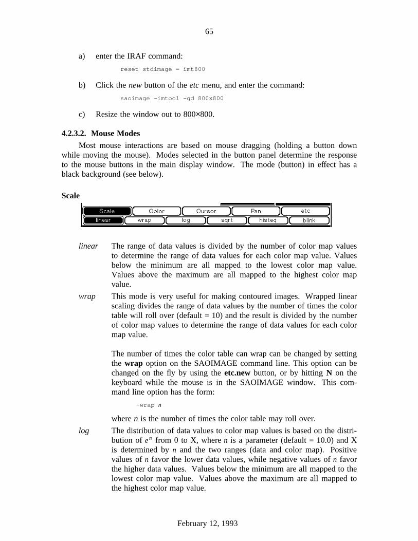
65

a) enter the IRAF command:

reset stdimage = imt800

b) Click the new button of the etc menu, and enter the command:

saoimage -imtool -gd 800x800

c) Resize the window out to 800×800.

4.2.3.2. Mouse Modes

Most mouse interactions are based on mouse dragging (holding a button downwhile moving the mouse). Modes selected in the button panel determine the responseto the mouse buttons in the main display window. The mode (button) in effect has ablack background (see below).

Scale

.

linear The range of data values is divided by the number of color map valuesto determine the range of data values for each color map value. Valuesbelow the minimum are all mapped to the lowest color map value.Values above the maximum are all mapped to the highest color mapvalue.

wrap This mode is very useful for making contoured images. Wrapped linearscaling divides the range of data values by the number of times the colortable will roll over (default = 10) and the result is divided by the numberof color map values to determine the range of data values for each colormap value.

The number of times the color table can wrap can be changed by settingthe wrap option on the SAOIMAGE command line. This option can bechanged on the fly by using the etc.new button, or by hitting N on thekeyboard while the mouse is in the SAOIMAGE window. This com-mand line option has the form:

-wrap n

where n is the number of times the color table may roll over.

log The distribution of data values to color map values is based on the distri-bution of e n from 0 to X, where n is a parameter (default = 10.0) and Xis determined by n and the two ranges (data and color map). Positivevalues of n favor the lower data values, while negative values of n favorthe higher data values. Values below the minimum are all mapped to thelowest color map value. Values above the maximum are all mapped tothe highest color map value.

February 12, 1993

66

The exponent n may be changed by setting the -log option on theSAOIMAGE command line. This option has the form:

-log n

where n is the exponent. This option can be changed on the fly by using theetc.new button, or by hitting N on the keyboard while the mouse is in theSAOIMAGE window.

sqrt The distribution of data values to color map values is based on the distri-bution of X (1/n) from 0 to 1, where n is a parameter (the default is 2.0)and X varies from 0 to 1 in steps determined by the number of color mapvalues. Values of n greater than 1 favor the lower data values, whilevalues of n less than 1 favor the higher data values (negative values and0 are not allowed). Values below the minimum are all mapped to thelowest color map value. Values above the maximum are all mapped tothe highest color map value.

The exponent n may be changed by setting the -sqrt option on theSAOIMAGE command line, of the form:

-sqrt n

where n is the inverse of the exponent. This option can be changed on the flyby using the etc.new button, or by hitting N on the keyboard while the mouseis in the SAOIMAGE window.

histeq Histogram equalization is a process whereby each range is adjusted withrespect to the others, until each range has about the same number ofpixel occurrences in the image, thus maximizing the information in thedisplay. This usually produces a dramatic improvement in the amount ofvisible detail in the display.

The drawback of histogram equalization is that the ranges can varygreatly in size, thus a difference between two adjacent color map valuesmay represent a big or a small difference in data values, with much irre-gularity from one step to the next

blink The display, as it currently appears in the main display window, can bestored by the workstation’s display server by clicking on the blink but-ton in the scale submenu. Three separate images can be saved, each oneassociated with a different mouse button. Each saved display is associ-ated with the mouse button used to click on the blink button, andreplaces any previous image associated with that mouse button. Thesaved display image can be redisplayed when in scale mode by pressingits mouse button while the mouse pointer is in the display window.

February 12, 1993

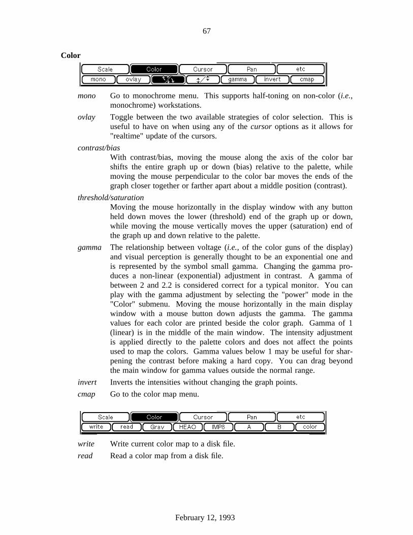
67

Color

.

mono Go to monochrome menu. This supports half-toning on non-color (i.e.,monochrome) workstations.

ovlay Toggle between the two available strategies of color selection. This isuseful to have on when using any of the cursor options as it allows for"realtime" update of the cursors.

contrast/biasWith contrast/bias, moving the mouse along the axis of the color barshifts the entire graph up or down (bias) relative to the palette, whilemoving the mouse perpendicular to the color bar moves the ends of thegraph closer together or farther apart about a middle position (contrast).

threshold/saturationMoving the mouse horizontally in the display window with any buttonheld down moves the lower (threshold) end of the graph up or down,while moving the mouse vertically moves the upper (saturation) end ofthe graph up and down relative to the palette.

gamma The relationship between voltage (i.e., of the color guns of the display)and visual perception is generally thought to be an exponential one andis represented by the symbol small gamma. Changing the gamma pro-duces a non-linear (exponential) adjustment in contrast. A gamma ofbetween 2 and 2.2 is considered correct for a typical monitor. You canplay with the gamma adjustment by selecting the "power" mode in the"Color" submenu. Moving the mouse horizontally in the main displaywindow with a mouse button down adjusts the gamma. The gammavalues for each color are printed beside the color graph. Gamma of 1(linear) is in the middle of the main window. The intensity adjustmentis applied directly to the palette colors and does not affect the pointsused to map the colors. Gamma values below 1 may be useful for shar-pening the contrast before making a hard copy. You can drag beyondthe main window for gamma values outside the normal range.

invert Inverts the intensities without changing the graph points.

cmap Go to the color map menu.

.

write Write current color map to a disk file.

read Read a color map from a disk file.

February 12, 1993

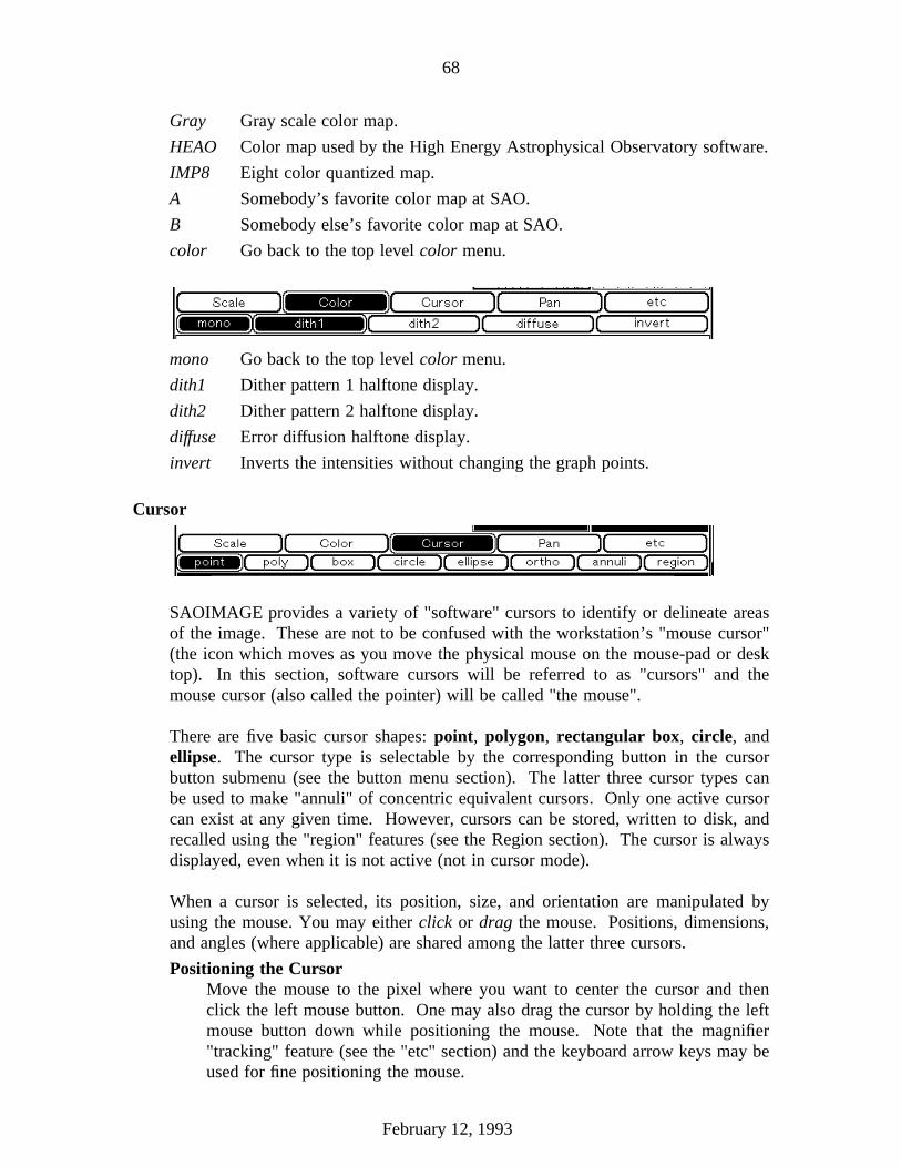
68

Gray Gray scale color map.

HEAO Color map used by the High Energy Astrophysical Observatory software.

IMP8 Eight color quantized map.

A Somebody’s favorite color map at SAO.

B Somebody else’s favorite color map at SAO.

color Go back to the top level color menu.

.

mono Go back to the top level color menu.

dith1 Dither pattern 1 halftone display.

dith2 Dither pattern 2 halftone display.

diffuse Error diffusion halftone display.

invert Inverts the intensities without changing the graph points.

Cursor

.

SAOIMAGE provides a variety of "software" cursors to identify or delineate areasof the image. These are not to be confused with the workstation’s "mouse cursor"(the icon which moves as you move the physical mouse on the mouse-pad or desktop). In this section, software cursors will be referred to as "cursors" and themouse cursor (also called the pointer) will be called "the mouse".

There are five basic cursor shapes: point, polygon, rectangular box, circle, andellipse. The cursor type is selectable by the corresponding button in the cursorbutton submenu (see the button menu section). The latter three cursor types canbe used to make "annuli" of concentric equivalent cursors. Only one active cursorcan exist at any given time. However, cursors can be stored, written to disk, andrecalled using the "region" features (see the Region section). The cursor is alwaysdisplayed, even when it is not active (not in cursor mode).

When a cursor is selected, its position, size, and orientation are manipulated byusing the mouse. You may either click or drag the mouse. Positions, dimensions,and angles (where applicable) are shared among the latter three cursors.

Positioning the CursorMove the mouse to the pixel where you want to center the cursor and thenclick the left mouse button. One may also drag the cursor by holding the leftmouse button down while positioning the mouse. Note that the magnifier"tracking" feature (see the "etc" section) and the keyboard arrow keys may beused for fine positioning the mouse.

February 12, 1993

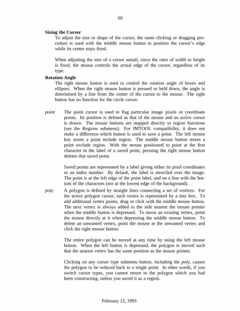
69

Sizing the CursorTo adjust the size or shape of the cursor, the same clicking or dragging pro-cedure is used with the middle mouse button to position the cursor’s edgewhile its center stays fixed.

When adjusting the size of a cursor annuli, since the ratio of width to heightis fixed, the mouse controls the actual edge of the cursor, regardless of itstype.

Rotation AngleThe right mouse button is used to control the rotation angle of boxes andellipses. When the right mouse button is pressed or held down, the angle isdetermined by a line from the center of the cursor to the mouse. The rightbutton has no function for the circle cursor.

point The point cursor is used to flag particular image pixels or coordinatepoints. Its position is defined as that of the mouse and no active cursoris drawn. The mouse buttons are mapped directly to region functions(see the Regions submenu). For IMTOOL compatibility, it does notmake a difference which button is used to save a point. The left mousekey stores a point include region. The middle mouse button stores apoint exclude region. With the mouse positioned to point at the firstcharacter in the label of a saved point, pressing the right mouse buttondeletes that saved point.

Saved points are represented by a label giving either its pixel coordinatesor an index number. By default, the label is stenciled over the image.The point is at the left edge of the point label, and on a line with the bot-tom of the characters (not at the lowest edge of the background).

poly A polygon is defined by straight lines connecting a set of vertices. Forthe active polygon cursor, each vertex is represented by a tiny box. Toadd additional vertex points, drag or click with the middle mouse button.The next vertex is always added to the side nearest the mouse pointerwhen the middle button is depressed. To move an existing vertex, pointthe mouse directly at it when depressing the middle mouse button. Todelete an unwanted vertex, point the mouse at the unwanted vertex andclick the right mouse button.

The entire polygon can be moved at any time by using the left mousebutton. When the left button is depressed, the polygon is moved suchthat the nearest vertex has the same position as the mouse pointer.

Clicking on any cursor type submenu button, including the poly, causesthe polygon to be reduced back to a single point. In other words, if youswitch cursor types, you cannot return to the polygon which you hadbeen constructing, unless you saved it as a region.

February 12, 1993

70

box Rectangular cursor.

circle Circular cursor.

ellipse Elliptical cursor.

ortho Reset rotation angle to 0.

annulii Annuli of box, circle, and ellipse cursors are available. Set the cursor tothe desired shape and angle before selecting the annuli feature, as thesecannot be changed once the annuli feature has been selected.

Annuli are sized by clicking or dragging with the middle mouse button.When the middle mouse button is first depressed, three possible eventsmay occur:

a) If the mouse is between existing annuli or not too far from an exist-ing annulus, a new annulus will be created sized by the mouse posi-tion.

b) If the mouse is well outside the existing cursor annuli, a new cursoris created with a radius that is initially incremented from the outerannulus by the same increment as that between the outer two annuli(or the annulus and the center if there is only one annulus). A com-parable situation applies when the mouse is well inside the inner-most annulus. However, once the annulus is created, if you proceedto drag the mouse with the middle mouse button down, the size ofthe new annulus reverts to being controlled by the mouse.

c) If the mouse is pointing at the edge of an existing annulus, thatannulus will be "grabbed" for sizing.

To delete an unwanted annulus, point the mouse at or near the unwantedannulus and click the right mouse button.

All of the annuli are forgotten when any cursor submenu button isselected, or reselected. The annuli button itself toggles between on andoff.

region Go into the region submenu.

.

A region is a cursor which has been stored. SAOIMAGE cursors can be stored,recalled, written to disk, and read from disk using the region features. Regioncontrols work only when SAOIMAGE is in cursor mode. Regions were designedfor use with SAO’s PROS/IRAF image analysis software, but they can be gen-erally useful.

February 12, 1993

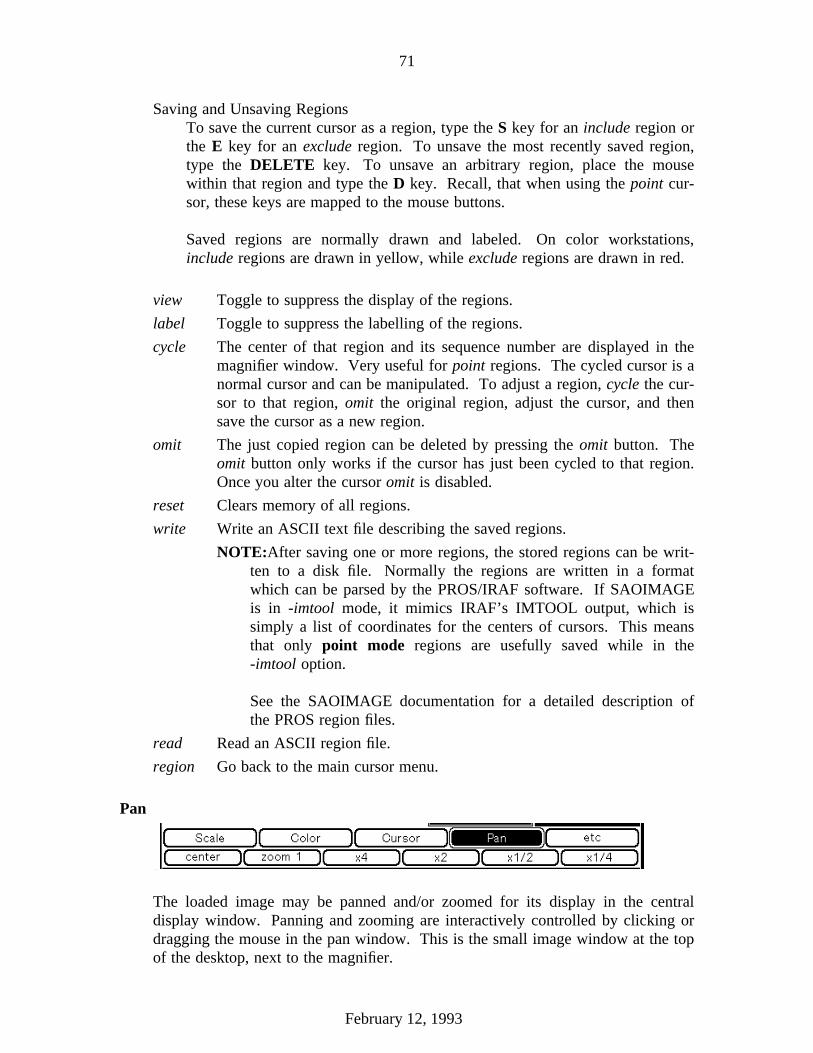
71

Saving and Unsaving RegionsTo save the current cursor as a region, type the S key for an include region orthe E key for an exclude region. To unsave the most recently saved region,type the DELETE key. To unsave an arbitrary region, place the mousewithin that region and type the D key. Recall, that when using the point cur-sor, these keys are mapped to the mouse buttons.

Saved regions are normally drawn and labeled. On color workstations,include regions are drawn in yellow, while exclude regions are drawn in red.

view Toggle to suppress the display of the regions.

label Toggle to suppress the labelling of the regions.

cycle The center of that region and its sequence number are displayed in themagnifier window. Very useful for point regions. The cycled cursor is anormal cursor and can be manipulated. To adjust a region, cycle the cur-sor to that region, omit the original region, adjust the cursor, and thensave the cursor as a new region.

omit The just copied region can be deleted by pressing the omit button. Theomit button only works if the cursor has just been cycled to that region.Once you alter the cursor omit is disabled.

reset Clears memory of all regions.

write Write an ASCII text file describing the saved regions.

NOTE:After saving one or more regions, the stored regions can be writ-ten to a disk file. Normally the regions are written in a formatwhich can be parsed by the PROS/IRAF software. If SAOIMAGEis in -imtool mode, it mimics IRAF’s IMTOOL output, which issimply a list of coordinates for the centers of cursors. This meansthat only point mode regions are usefully saved while in the-imtool option.

See the SAOIMAGE documentation for a detailed description ofthe PROS region files.

read Read an ASCII region file.

region Go back to the main cursor menu.

Pan

.

The loaded image may be panned and/or zoomed for its display in the centraldisplay window. Panning and zooming are interactively controlled by clicking ordragging the mouse in the pan window. This is the small image window at the topof the desktop, next to the magnifier.

February 12, 1993

72

The pan window shows the entire area of the loaded image. A box cursor in thepan window shows the area of the image currently being displayed in the maindisplay window. This box can be moved and sized just like the regular box cursor(but without angular rotation control).

The left mouse button controls the location of the center of the box (the displayimage). The middle button controls the edge of the box, for the given center, thusdetermining its size.

When the mouse is in the pan window, the area under the mouse pointer can bemagnified in the magnifier by pressing or holding the shift key on the keyboard.The T key table also works with the pointer in the pan window. The arrow keyscan be used for fine positioning.

The same types of interactions as those used in the pan window can be performedin the main display window. Clicking or dragging with the left button controls thecenter of the display. Clicking or dragging with the middle button determines thezoom factor. The box cursor in the pan window tracks these manipulations as themouse is dragged in the display window.

center Centers the display on the image.

zoom 1 Set zoom to one display pixel per image pixel.

x4 Zoom factor increase by 4.

x2 Zoom factor increase by 2.

x1/2 Zoom factor decrease by 1/2.

x1/4 Zoom factor decrease by 1/4.

Etc

.

new Change the SAOIMAGE command line command.

track Track the mouse cursor in the display window, showing a magnified areain the magnify window.

coord Track the coordinates of the mouse in the display window.

verb Print any verbose output to the terminal window from which SAOIM-AGE was executed.

print Make a hardcopy of the main image display on a Postscript printer.

On color workstations, the image is read from the screen and includesany graphics which may be showing. The image also includes the upperportion of SAOIMAGE (the title area and two auxiliary windows). Bydefault, the buttons are not included, but they may be included by firstusing the -lprbuttons option switch on the command line.

February 12, 1993

73

The output file can be directed anywhere by setting an environment vari-able called R_DISPOSE. The R_DISPOSE string is a format statementfor a sprintf which creates the UNIX command, where ’%s’ will bereplaced by its temporary file name. The default is "lpr -Plw -r %s".The -r in the print statement deletes the Postscript file after beingprinted. One could, for example, set R_DISPOSE to "mv %s/tmp/foo.ps" to save the file for later use.

If no R_DISPOSE environment variable is set, SAOIMAGE looks for aPRINTER environment variable. If one is set, the hardcopy will be sentto that printer. If no PRINTER variable is found, the default destinationis lw.

raise Bring the SAOIMAGE window to the foreground.

QUIT Exit SAOIMAGE.

4.2.3.3. Keyboard Modes

Many of the keys on the keyboard are mapped to perform useful functions. Strik-ing the key results in an immediate response. The response may be dependent on thewindow in which the mouse cursor is positioned. Some responses are also dependenton the main menu mode (i.e., cursor). Both upper and lower case are mapped the same.

Mapped key commands

Up, Down, Left and Right ArrowsThese can be used to move the mouse cursor one screen pixel in the givendirection. This facilitates fine positioning and works in all windows and allmodes.

R or rRaise all SAOIMAGE windows to the front of any other windows on thescreen. The ’A’ key also performs this function.

A or aRaise and redraw the display windows.

N or nEnter new command-line arguments. All of the command line argumentswhich affect selection and display of an image can be used. Someconfiguration arguments (e.g. -d, -g, and -G) are not effective at this time.

T or tWhen the mouse is in the main display window or the pan window, thisprints a table of the pixel values surrounding the current mouse position. Thetable is printed in the terminal window from which SAOIMAGE was called.

S or sWhen in cursor mode, and the mouse is in the display window, the currentcursor is saved as a region (of type include).

February 12, 1993

74

E or eWhen in cursor mode, and the mouse is in the display window, the currentcursor is saved as a region (of type exclude).

D or dWhen in cursor mode, and the mouse is in the display window, the smallestregion which encloses the mouse is deleted.

DELETEWhen in cursor mode, and the mouse is in the display window, the mostrecently saved region is deleted.

Modifier Keys

ShiftHolding the shift key down toggles the track and coord options.

� If no tracking was selected and the mouse is in either the main displaywindow or the pan window, touching the shift key will update themagnifier window to the current mouse location. If the mouse is in themain display window, the coordinates and pixel value will also appearin the upper right, above the buttons.

� If you are in Color mode and dragging the mouse with a button down ineither the main or color graph window, the graph will be updated to thecurrent state of the color table.

� By continuing to hold the shift key down, tracking will continue toupdate as you move the mouse.

� If you were tracking before touching the shift key, pressing the shift keywill suspend tracking, enabling you to preserve the existing trackingdisplays while moving the mouse.

Caps or ShiftLockToggling to caps mode by using the Caps or shift lock key has the sameeffect as holding the shift key down. When using this option, you may needto toggle it off to make normal text entry in the pop-up or terminal window.

ControlWhen manipulating the color map in the main display window, holding thecontrol key down restricts the affect to only the color(s) corresponding to themouse button(s) being pressed (left=red, middle=green, right=blue).

Pop-up Text and Numeric InputWhen SAOIMAGE needs string input such as the name of a file or new commandline arguments, it presents a pop-up window for you to type in. The line startswith a default already typed in. Many keyboard editor keys are recognized,including the arrows. The popup window also recognizes many EMACS style lineedit commands. For numeric input, the typed input must be in acceptable integeror real (where allowed) format. Multiple entries, when desired, must be separatedby spaces, commas, or tabs. The input is taken when the user strikes the returnkey. The following are some of the more useful EMACS editing options.

February 12, 1993

75

CTRL-A: Move text cursor to beginning of lineCTRL-B: Move the text cursor back one character (backspace)CTRL-C: Abort the interaction and return to SAOIMAGECTRL-D: Delete the character under the text cursorCTRL-E: Move the text cursor to the end of the lineCTRL-F: Move forward one spaceCTRL-G: Clear escape if just typedCTRL-K: Delete all characters from the text cursor to the end of the lineCTRL-N: Recall next input line (clear input line if no next in buffer)CTRL-P: Recall prior input lineDelete: Delete character before the text cursorescape-B: Move to beginning of previous wordescape-D: Delete to end of next wordescape-F: Move to end of next word

February 12, 1993

76

4.2.4. Captain Video

The cv program (affectionately known as Captain Video) is used to control I 2S-likedisplay devices. It differs from most IRAF programs since it has its own prompt — asmiley face :) — and its own internal language (cryptic to say the least). While usingcv, no other IRAF or host system commands can be issued.

The following is a copy of the help page one would see if one types a ? to the cvprompt.

--- () : optional; [] : select one; N : number; C/F/Q : see belowb(link) N F (C Q) (F (C Q)..) blink (N = 10 is one second)c(ursor) [on off F] cursordi F (C Q) [on off] display imagedg C (F Q) [on off] display graphicse(rase) [N a(ll) g(raphics) F] erase (clear)m(atch) (o) F (C) (to) (F) (C) match (output) lookup tableo(ffset) C N offset color (N: 0 to +- 4095)p(an) (F) pan imagesps(eudo) (o) (F C) (rn sn) pseudo color mapping

rn/sn: random n/seed nr(ange) N (C) (N C ...) scale image (N: 1-8)re(set) [r i t a] reset display

registers/image/tables/allsn(ap) (C) snap a pictures(plit) [c o px,y nx,y] split picturet(ell) tell display statew(indow) (o) (F C) window (output) frameswr(ite) [F C] text write text to frame/graphicsz(oom) N (F) zoom frames (N: 1-8)x or q exit/quit--- C: letter c followed by r/g/b/a or, for snap r,g,b,m,bw,rgb,--- or for dg r/g/b/y/p/m/w, as ’cr’, ’ca’, or ’cgb’--- F: f followed by a frame number or ’a’ for all--- Q: q followed by quadrant number or t,b,l,r for top, bottom,...

Commands are distinguished by their first letter, except for a few instances wherethe second letter is needed. The rest of the command name can be typed if you wish.Commands often require specification of frame numbers, colors, quadrants, or numericvalues. In most cases, the order is unimportant, but, zoom, for instance, does requirethe zoom power right after the command name. The order given in the help commandwill always work.

Frame SpecificationA frame list is indicated in the help listing with a F. This is to be replaced in thetyped command by an f followed (no spaces) by a list of the pertinent imageplanes. Thus, f1 means frame 1 while f42 means frames 4 and 2. Thespecification fa means all frames. If the frame specification is optional, omittingthe frame list is the same as typing fa; that is, operate on all frames.

Color SpecificationA color specification is indicated in the help listing with a C. A colorspecification is a c followed by a set of letters. The letter a means all, just as inthe frame specification. The letters r, b, and g are the other possibilities for allcommands other than dg and snap. For displaying graphics planes (dg), the otherpossibilities are y, p, m, w which stand for yellow, purple, mauve, and white. An

February 12, 1993

77

omitted color specification is the same as all colors.

Quadrant SpecificationA quadrant specification is indicated in the help listing with a Q. Quadrants aregiven by a q followed by numbers from the set one through four, or the letter a asin the frame and color cases. Quadrants are numbered in the standard way, withthe upper right being 1, the upper left 2, etc. Adjacent quadrants may be refer-enced by t, b, l, and r, standing for top, bottom, left, and right. An omitted qua-drant specification is the same as all quadrants. Quadrants are effective only if thesplit screen command has set the split point to something other than the "origin."

The following are explanations and/or examples of the more frequently used com-mands:

blink N F (C Q) (F C Q)

The command

:) b 10 f12

blinks frames 1 and 2 at a rate of 1 second.

The command

:) b 20 f1 cr q1 f2 cb q1 f4 cg q1

blinks quadrant 1 of frames 1, 2 and 4 at a rate of 2 seconds, using only red forframe 1, blue for frame 2 and green for frame 3.

cursor [on off F]

It has been the author’s experience that this is actually two commands. The com-mand

:) c on f1

only turns the cursor on for frame 1, but does not go into coordinate readoutmode. This is useful for toggling the cursor on and off when taking pictures of thedisplay screen or making dicomeds where you do not want the cursor in the pic-ture.

To turn on the coordinate readout mode, one must type in more of the word cur-sor than just the first letter. The program then responds as shown below:

:) cu on f1Press <cr> for each read; any key but <sp> and then <cr> to exit.

frame 1, pixel (131,108): 255frame 1, pixel (62,226): 132l<cr>:)

There are two items to note at this point:

February 12, 1993

78

1) The value of the pixel (listed on the right) is, unfortunately, the outputlookup-table value, and not the actual value of the pixel in the image.

2) The pixel coordinates are given with respect to the lower left corner of thedisplay, and therefore not necessarily the image. If the image is smaller thanthe display window, then offsets must be determined.

di F (C Q) [on off]

This command turns frames on (or off). Turning a frame off does not erase it. Aframe need not have all colors turned on, nor appear in all quadrants of a splitscreen display.

For example, to get a real color display, where frame 1 contains the red image,frame 2 is the blue image and frame 3 is the green image the following commandswould be used:

:) di fa off:) di f1 cr on:) di f2 cb on:) di f3 cg on

dg C (F Q) [on off]

This command turns specific graphics planes on or off. For the I 2S display, nei-ther the frame nor the quadrant parameters are relevant.

This is useful for toggling graphics overlays (such as that produced by write) onand off. For example, the command sequence

:) dg ca off:) dg cr on

turns on the red graphics plane only.

erase [F all graphics]

This command erases the specified frame, or all the graphics planes, or all dataplanes.

pan (F)

This command connects the trackball to the specified frames and allows the user tomove (pan/roam/scroll) the image about the screen. This function is automaticallyinvoked whenever the zoom factor is changed.

pseudo (o) (F C) (rn sn)

This command provides pseudo-coloring capabilities. Pseudo-color maps are usu-ally best done in the output tables, rather than in the look-up tables associated withparticular frames; hence, ps o is the more likely invocation of the start of the com-mand line.

Two mappings are provided.

February 12, 1993

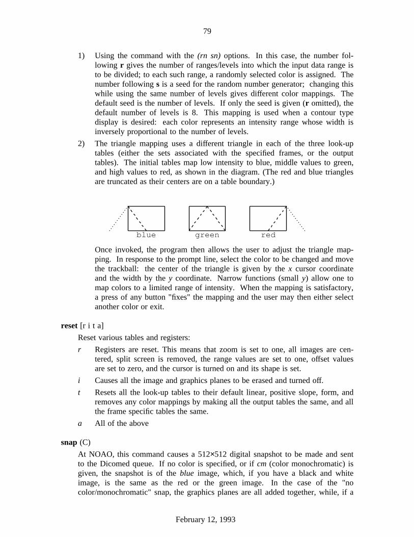
79

1) Using the command with the (rn sn) options. In this case, the number fol-lowing r gives the number of ranges/levels into which the input data range isto be divided; to each such range, a randomly selected color is assigned. Thenumber following s is a seed for the random number generator; changing thiswhile using the same number of levels gives different color mappings. Thedefault seed is the number of levels. If only the seed is given (r omitted), thedefault number of levels is 8. This mapping is used when a contour typedisplay is desired: each color represents an intensity range whose width isinversely proportional to the number of levels.

2) The triangle mapping uses a different triangle in each of the three look-uptables (either the sets associated with the specified frames, or the outputtables). The initial tables map low intensity to blue, middle values to green,and high values to red, as shown in the diagram. (The red and blue trianglesare truncated as their centers are on a table boundary.)

....

........

. .............blue green red

Once invoked, the program then allows the user to adjust the triangle map-ping. In response to the prompt line, select the color to be changed and movethe trackball: the center of the triangle is given by the x cursor coordinateand the width by the y coordinate. Narrow functions (small y) allow one tomap colors to a limited range of intensity. When the mapping is satisfactory,a press of any button "fixes" the mapping and the user may then either selectanother color or exit.

reset [r i t a]

Reset various tables and registers:

r Registers are reset. This means that zoom is set to one, all images are cen-tered, split screen is removed, the range values are set to one, offset valuesare set to zero, and the cursor is turned on and its shape is set.

i Causes all the image and graphics planes to be erased and turned off.

t Resets all the look-up tables to their default linear, positive slope, form, andremoves any color mappings by making all the output tables the same, and allthe frame specific tables the same.

a All of the above

snap (C)

At NOAO, this command causes a 512×512 digital snapshot to be made and sentto the Dicomed queue. If no color is specified, or if cm (color monochromatic) isgiven, the snapshot is of the blue image, which, if you have a black and whiteimage, is the same as the red or the green image. In the case of the "nocolor/monochromatic" snap, the graphics planes are all added together, while, if a

February 12, 1993

80

real color is given, only the graphics planes that have some of that color areincluded in the image.

See the cv help pages for hints on dealing with color images.

split [c o px,y nx,y]

This command sets the split screen point.

c Sets the split point in the center of the screen.

o Resets the split point to the origin (i.e., the split position that corresponds tono split screen).

px,y Specifies the split point in integer pixels.

nx,y Specifies the split point in NDC units (which range from 0 though 1.0), inwhich the coordinates are decimal fractions.

tell

Displays what it knows about the display status.

window [F C] text

This is most commonly used without the color option to adjust the contrast. Win-dowing is performed by applying a linear mapping to the output look-up tables (ifoption o is used) or to the frame specific tables. The mapping is controlled by thetrackball, with the y cursor coordinate supplying the slope of the map, and x theoffset. If different mappings are given to each color, a form of pseudo-color isgenerated.

write [F C] text

This command writes the given text into either an image plane (or planes) or intothe specified color graphics bit plane(s). The user is prompted to place the cursorat the (lower left) corner of the text, which is then written to the right in Romanfont. The user is also asked for a text size (default 1.0).

Note, it is much safer to write into the graphics planes. If a mistake is make, oneonly needs to erase the appropriate plane rather that redisplay the image(s) and re-window, etc.

zoom N (F)

This command zooms the display to the power given by N. For the I 2S, the powermust be 1,2,4, or 8; anything else is changed to the next lower legal value. Oncethe zoom has taken place, the pan routine is called for the specified frames.

Note that some display devices (e.g., I 2S model 70) cannot zoom different planesby different factors (i.e., the same zoom factor is applied to all planes together).

February 12, 1993

81

4.2.5. Displaying Images Over the IRAF Network

The IRAF network may be used for image display. There are basically two waysto make use of the network.

1) If the local and remote machines are compatible in terms of file structure (e.g.,both are Suns) then one only needs to set an environment variable pointing to theremote directory.

For example, to display images that reside on Orion (a Sun 4) on Lacerta (a Sun3/60) from Lacerta,

tv> set ed = "orion!/u2/anderson/prototype/"tv> disp ed$image1 1

2) If the local and remote machines are incompatible (e.g., a DECstation 3100 and aSun 3/60) then it is necessary to login to the remote machine (e.g., from anotherwindow), startup IRAF specifying the node and imtool configuration.

For example, to display an image on Lacerta (a Sun 3/60) while remotely loggedinto Equuleus (a DECstation 3100) and running IRAF,

tv> set node = lacertatv> reset stdimage = imt512tv> disp dev$pix 1

4.3. IRAF Graphics (PLOT)

The PLOT package contains the generic image and list plotting tasks, as well astasks to send device independent plotfiles to various hardcopy devices. The followingis the help menu for the PLOT package:

February 12, 1993

82

plot.:calcomp - Plot metacode on a Calcomp pen plottercontour - Make a contour plot of an imagecrtpict - Generate greyscale plots of IRAF images

gkidecode - Decode metacode on the standard outputgkidir - Directory listing of metacode file

gkiextract - Extract individual frames from metacode filegkimosaic - Condense metacode frames to fit on one page

graph - Graph one or more image sections or listshafton - Generate half-tone plots of an imageimdkern - Image display device (IMD) graphics kernelimplot - Plot lines and columns of images using cursors

nsppkern - Plot metacode on a NSPP (NCAR) plotter devicepcol - Plot a column of an imagepcols - Plot the average of a range of image columnsprow - Plot a line (row) of an imageprows - Plot the average of a range of image lines

pvector - Plot an arbitrary vector in a 2D imagesgidecode - Decode an SGI format metacode file

sgikern - Simple graphics interface (SGI) graphics kernelshowcap - Show and decode graphcap entriesstdgraph - Plot metacode on the standard graphics devicestdplot - Plot metacode on the standard plotter devicesurface - Make a surface plot of an imagevelvect - Plot representation of a velocity field

The tasks calcomp and crtpict seem to be NOAO specific (in the sense that theauthor is not aware of any other IRAF site using Calcomp plotters or DICOMED pho-tos). The tasks gkidecode, nsppkern, sgidecode, sgikern and showcap are usedmainly by programmers to help debug graphics code. These tasks will not be discussedfurther in this document.

The tasks pcol, pcols, prow and prows are used to plot rows and columns (oraverages of rows and columns) of images. These tasks mimic tasks (of the samenames) that reside in the KPNO Mountain Forth system. The task implot supercedesthese and so they will not be discussed here.

4.3.1. IMPLOT

implot is an interactive, cursor driven task for examining images by plotting thelines and columns or the averages of lines and columns. The following is the parameterlist for implot

pl> lpar implotimage = image to be plottedline = line to be plotted

(coords = "") graphics cursor input(device = "stdgraph") graphics device for plots

(mode = "ql")

If the parameter line is given, that image line will be plotted when the task is first run,otherwise, the central line is plotted. Then cursor mode is entered and keystrokes maybe used to generate additional line and column plots. The following plot is the result ofthe command (note that the cursor is not shown in any hardcopy output):

February 12, 1993

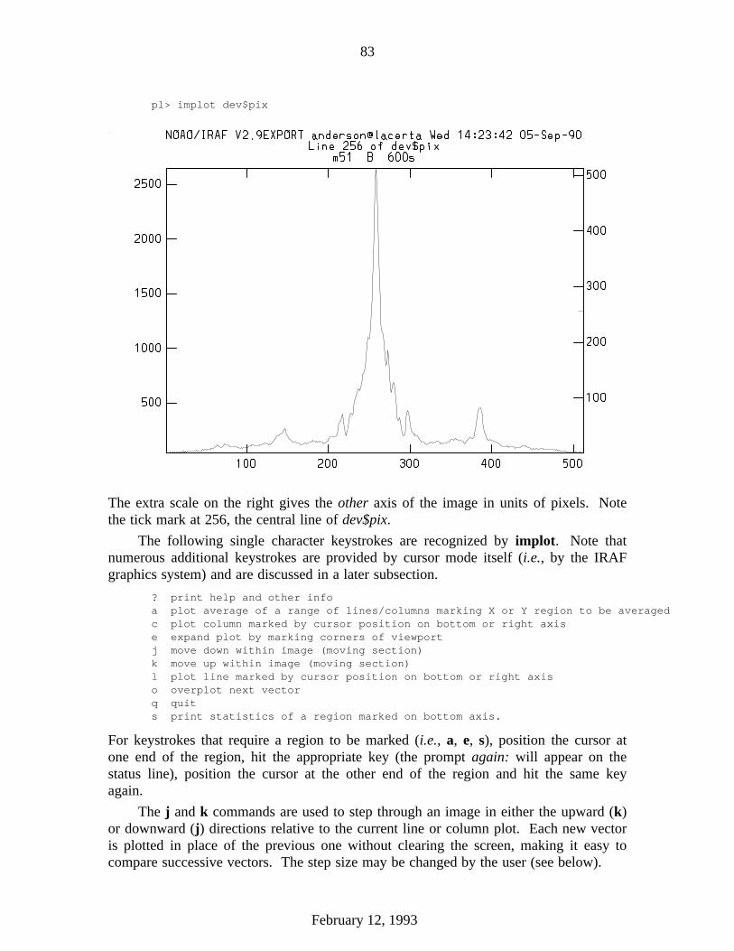
83

pl> implot dev$pix

.

The extra scale on the right gives the other axis of the image in units of pixels. Notethe tick mark at 256, the central line of dev$pix.

The following single character keystrokes are recognized by implot. Note thatnumerous additional keystrokes are provided by cursor mode itself (i.e., by the IRAFgraphics system) and are discussed in a later subsection.

? print help and other infoa plot average of a range of lines/columns marking X or Y region to be averagedc plot column marked by cursor position on bottom or right axise expand plot by marking corners of viewportj move down within image (moving section)k move up within image (moving section)l plot line marked by cursor position on bottom or right axiso overplot next vectorq quits print statistics of a region marked on bottom axis.

For keystrokes that require a region to be marked (i.e., a, e, s), position the cursor atone end of the region, hit the appropriate key (the prompt again: will appear on thestatus line), position the cursor at the other end of the region and hit the same keyagain.

The j and k commands are used to step through an image in either the upward (k)or downward (j) directions relative to the current line or column plot. Each new vectoris plotted in place of the previous one without clearing the screen, making it easy tocompare successive vectors. The step size may be changed by the user (see below).

February 12, 1993

84

Successive vectors may be overplotted by typing an o and then any other com-mand. A range of linetypes are used if the device supports them to make the curveseasier to distinguish. The position of each line is marked on the right axis with a smalltick to document the coordinates of the curves.

In addition to the single keystroke commands, the following ":" escape commandsare provided:

:a N set number of lines or columns to average (default = 1):c N [M] plot column N [average of columns N to M]:i imagename open a new image for input:l N [M] plot line N [average of lines N to M]:o overplot:log+ log scale in Y:log- turn off log scale in Y:step N set step size for j,k (default = 0.1 * NAXIS2):solid overplot with solid, not dashed, lines:x x1 x2 fix range in X (call with no args to unfix):y y1 y2 fix range in Y (call with no args to unfix)

The :c and :l commands are identical to the keystroke commands except that thecolumn or line position is explicitly entered. If two numbers are entered, then an aver-age of rows/columns ranging between the entered values is plotted.

If one always wants to see the average of a certain number of rows/columns, thenthe :a command can be used to set that number. The averaging factor entered with :awill apply to all subsequent line and column plots, as well as plots generated by j andk.

The :x and :y commands may be used to fix the plotting scale in either X or Y,(i.e., to disable autoscaling) also to return to autoscale mode (when used with no argu-ments). Once the scale is fixed on an axis it remains fixed until either the fix scalecommand is repeated without any arguments, or the e option is used to expand the plot(this causes the fixed scale to be lost). Plotting different lines or columns or evenchanging images does not cause loss of fixed scaling.

The :i command is used to change images without having to exit and re-enterimplot. Note, if the image is larger than 2 dimensions (i.e., 3d) then to be sure that theproper band is being plotted one should explicitly give the correct image section whencalling implot or use :i (e.g., myimage[*,*,2]).

Note: When using a workstation, the mouse (i.e., cursor) must be in the graph win-dow when attempting to use the various keystroke or colon commands.

Example 4.3.26:This example shows overplots of row 173 between columns 30 and 70 in eachband of a GONG calibration image (256×252×3). This area of the image con-tains a feature that was noticed when the image was displayed and we want tosee how it behaves in each band. The following keystroke and colon com-mands produced the plot shown below from the initial command implotraw1, which defaulted to plotting the middle row of the first band.

February 12, 1993

85

:l 173:x 30 70:y 2.0e6 2.5e6:i raw1[*,*,2]o:l 173:i raw1[*,*,3]o:l 173

The plot below is the result after the last of the above commands was entered..

Adding annotation to the plot and getting the hardcopy will be discussed inlater sections.

4.3.2. GRAPH

graph is a non-interactive plotting task that may be used to examine images orcreate plots from lists of numbers. This task is more flexible than implot in the sensethat one may adjust scaling, axis titles, tick marks, etc., in order to make somewhat of apublication quality plot.† The following is the parameter listing for graph.

pl> lpar graphinput = list of images or list files to be graphed(wx1 = 0.) left world x-coord if not autoscaling(wx2 = 0.) right world x-coord if not autoscaling

† Full publication quality plotting capabilities similar to MONGO will be available in futureversions of IRAF.

February 12, 1993

86

(wy1 = 0.) lower world y-coord if not autoscaling(wy2 = 0.) upper world y-coord if not autoscaling(axis = 1) axis along which projection is to be taken

(transpose = no) transpose the x and y axes of the plot(pointmode = no) plot points instead of lines?

(marker = "box") point marker character?(szmarker = 0.005) marker size (0 for list input)

(logx = no) log scale x-axis(logy = no) log scale y-axis(box = yes) draw box around periphery of window

(ticklabels = yes) label tick marks(xlabel = "") x-axis label(ylabel = "") y-axis label(title = "imtitle") title for plot

(lintran = no) perform linear transformation of x axis(p1 = 0.) start input pixel value for lintran(p2 = 0.) end input pixel value for lintran(q1 = 0.) start output pixel value for lintran(q2 = 1.) end output pixel value for lintran(vx1 = 0.) left limit of device viewport (0.0:1.0)(vx2 = 0.) right limit of device viewport (0.0:1.0)(vy1 = 0.) bottom limit of device viewport (0.0:1.0)(vy2 = 0.) upper limit of device viewport (0.0:1.0)

(majrx = 5) number of major divisions along x grid(minrx = 5) number of minor divisions along x grid(majry = 5) number of major divisions along y grid(minry = 5) number of minor divisions along y grid

(append = no) append to existing plot?(device = "stdgraph") output device(round = no) round axes to nice values?(fill = yes) fill viewport vs enforce unity aspect ratio?(mode = "ql")

Lists and image sections may be mixed in the input list at will. If the curves arenot all the same length the plot will be scaled to the longest curve and all curves will beplotted left justified. If an image section operand has more than one dimension the pro-jection (average) along a designated axis will be computed and plotted. List input maybe taken from the standard input or from a file, and consists of a sequence of Y values,X and Y values, or X, Y, and marker size values, one pair of coordinates per line in thelist.

Example 4.3.27:The following example demonstrates the use of the lintran (and p & q) parametersto plot the frequency region 2000≤ν0≤5000µHz region of a solar oscillation powerspectrum.

pl> imhead m2150m2150[16385][real]: m-averaged spectrumpl> graph m2150 lint=yes p1=1 q1=0. p2=2 q2=0.406901 wx1=2000. wx2=5000. \>>> xlabel="Frequency (mircoHz)" ylab="Power" round+ \>>> title="M-averaged Spectrum (l=150)"

February 12, 1993

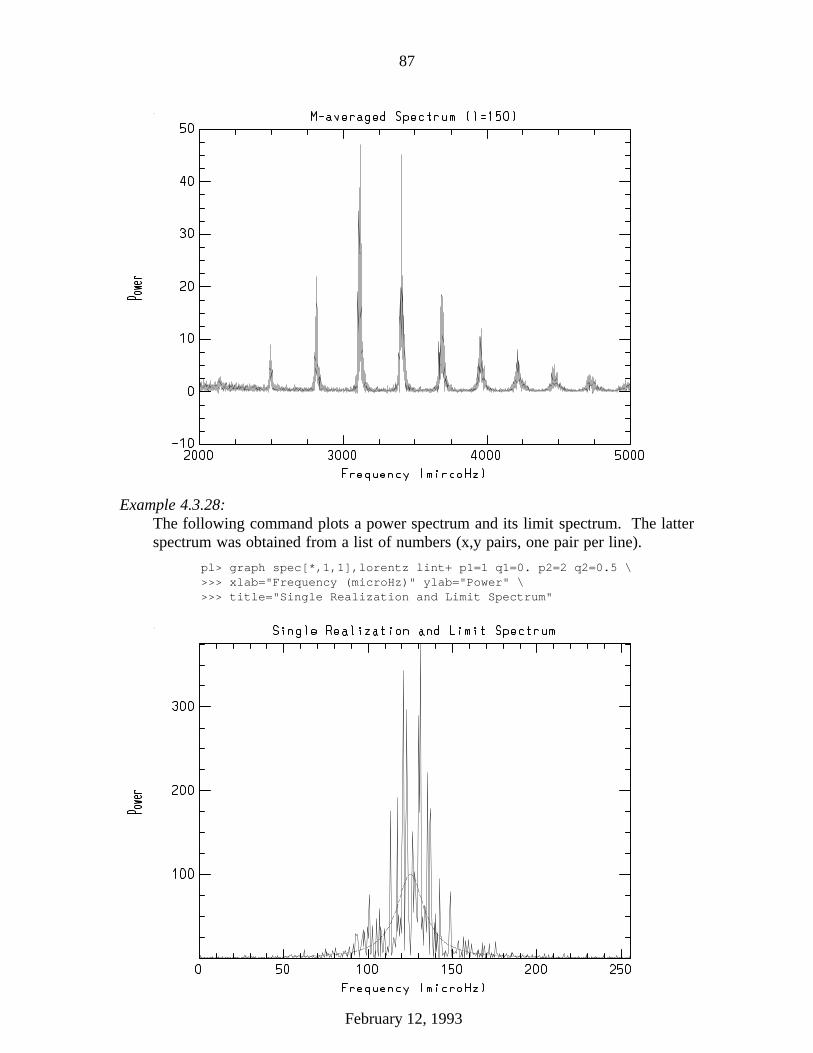
87

.

Example 4.3.28:The following command plots a power spectrum and its limit spectrum. The latterspectrum was obtained from a list of numbers (x,y pairs, one pair per line).

pl> graph spec[*,1,1],lorentz lint+ p1=1 q1=0. p2=2 q2=0.5 \>>> xlab="Frequency (microHz)" ylab="Power" \>>> title="Single Realization and Limit Spectrum"

.

February 12, 1993

88

graph may also be used to plot points and/or error bars.� The parameter marker determines the point shape ( "point", "box", "cross", "plus",

"circle", "hebar", "vebar", "hline", "vline" or "diamond").� The parameter szmarker is the size of a marker in NDC coordinates (0 to 1 spans

the screen). If zero and the input operand is a list, marker sizes are taken indivi-dually from the third column of each list element (ranging from 0 - 1). If positive,all markers are of size szmarker. If negative and the input operand is a list, thesize of a marker is the third column of each list element times the absolute valueof szmarker.

If the third column of a list contains positive numbers, they are interpreted as NDCmarker sizes, optionally scaled by the absolute value of szmarker. If you want the thirdcolumn of a list to be interpreted as WCS coordinates, indicating errors for example,the marker sizes should be entered as negative numbers.

Example 4.3.29:Use point mode, and marker sizes and shapes to plot points and error bars.

shape.dat error.dat1 1 1 1 1 -12 2 2 2 2 -23 3 3 3 3 -34 4 4 4 4 -45 5 5 5 5 -56 6 6 6 6 -67 7 7 7 7 -78 8 8 8 8 -89 9 9 9 9 -9

pl> graph shape.dat point+ mark="diamond" szm=-0.005 round+pl> graph error.dat point+ mark="vebar" szm=0. round+ app+

.

February 12, 1993

89

4.3.3. CONTOUR

contour produces a contour map of an image. The parameters are listed below:

pl> lpar contourimage = image or image section to be plotted(floor = 0.) minimum value to be contoured (0 if none)

(ceiling = 0.) maximum value to be contoured (0 if none)(zero = 0.) greyscale value of zero contour

(ncontours = 0) number of contours to be drawn (0 for default)(interval = 0.) contour interval (0 for default)

(nhi = -1) hi/low marking option: -1=omit, 0=mark h/l, 1=m(dashpat = 528) bit pattern for generating dashed lines(device = "stdgraph") output device(title = "imtitle") optional title

(preserve = yes) preserve aspect ratio of image?(label = yes) label major contours with their values?(fill = no) fill viewport regardless of device aspect ratio(xres = 64) resolution in x(yres = 64) resolution in y

(perimeter = yes) draw labelled perimeter around plot?(vx1 = 0.) NDC viewport x1(vx2 = 0.) NDC viewport x2(vy1 = 0.) NDC viewport y1(vy2 = 0.) NDC viewport y2

(subsample = no) Subsample (vs blockaverage) to decrease resolut(append = no) append to an old plot

(mode = "ql")

The most commonly adjusted parameters are floor, ceiling, zero, ncontours and interval.

Example 4.3.30:Contour the image raw1 (from Example 4.3.1), adjusting the floor, ceiling, andzero point. Note the feature in Example 1 can be seen here (50,173).

pl> cont raw1 floor=2.1e6 ceil=2.5e6 ncon=10 zero=2.3e6.

February 12, 1993

90

4.3.4. SURFACE

surface draws a pseudo-three dimensional perspective of an image section. Hid-den lines are removed. The surface may be viewed from any angle. The parameters ofsurface are:

pl> lpar surfaceimage = image or image section to be plotted(floor = 0.) minimum value to be plotted (0 if none)

(ceiling = 0.) maximum value to be plotted (0 if none)(angh = -33.) horizontal viewing angle, degrees(angv = 25.) vertical viewing angle, degrees

(device = "stdgraph") output device(title = "imtitle") optional title(label = no) label corner points of plot

(preserve = yes) preserve aspect ratio when decreasing resolutio(xres = 64) number of pixels resolution in x(yres = 64) number of pixels resolution in y

(subsample = no) subsample (vs block average) to reduce resoluti(append = no) append to an old plot

(mode = "ql")

Example 4.3.31:surface the first band of the image raw1, using the same floor and ceiling valuesas in the contour example above:

pl> surface raw1 floor=2.1e6 ceil=2.5e6 lab+

.

It is usually a good idea to turn label on, so that the orientation of the surface plot isimmediately apparent.

February 12, 1993

91

4.3.5. HAFTON

hafton draws a half tone picture of an IRAF image, where varying intensities inthe image are represented by areas of varying darkness on the plot. This can be a veryuseful task when an image display device is not available. The parameters of haftonare:

pl> lpar haftonimage = image or image section to be plotted

(z1 = 0.) minimum intensity to be mapped (0 if zmin)(z2 = 0.) maximum intensity to be mapped (0 if zmax)

(nlevels = 0) number of levels to be drawn (0 for default)(mapping_func = "linear") type of mapping

(contrast = 0.25) positive or negative contrast [+/-1]?(perimeter = yes) draw perimeter around plot?

(device = "stdgraph") output device(title = "imtitle") optional title

(preserve = yes) preserve aspect ratio when decreasing resolution(xres = 64) x resolution in pixels(yres = 64) y resolution in pixels(vx1 = 0.) NDC viewport x1(vx2 = 0.) NDC viewport x2(vy1 = 0.) NDC viewport y1(vy2 = 0.) NDC viewport y2(fill = no) fill viewport regardless of device aspect ratio

(subsample = no) subsample (vs block average) to reduce resolution(append = no) append to an old plot?

(mode = "ql"

The default number of greyscale levels (nlevels) is the maximum 16.

Several different mapping functions are available:

linearexponential - emphasizes high intensity values.logarithmic - emphasizes low intensity values.sinusoidal - emphasizes mid-range values.arcsine - extreme values emphasized at the expense of mid-range.crtpict - linear mapping centered on median intensity.

The slope of the function is modified by contrast.

The parameter contrast may be positive or negative contrast. Negative contrast is indi-cated by setting contrast to a negative number. The magnitude of contrast is notimportant unless mapping_function = crtpict in which case it is used in the samemanner as tv.display.

Note: When sending hafton plots to a hardcopy device (i.e., a Postscript printer) alarge number of instructions are generated, and therefore it may take manyminutes (e.g., a half-hour or so) for the printer to get the plot out.

Example 4.3.32:The following is a hafton of the first band of raw1 (i.e., the image used in theprevious two examples).

pl> hafton raw1 z1=2.2e6 z2=2.5e6 map=exp

February 12, 1993

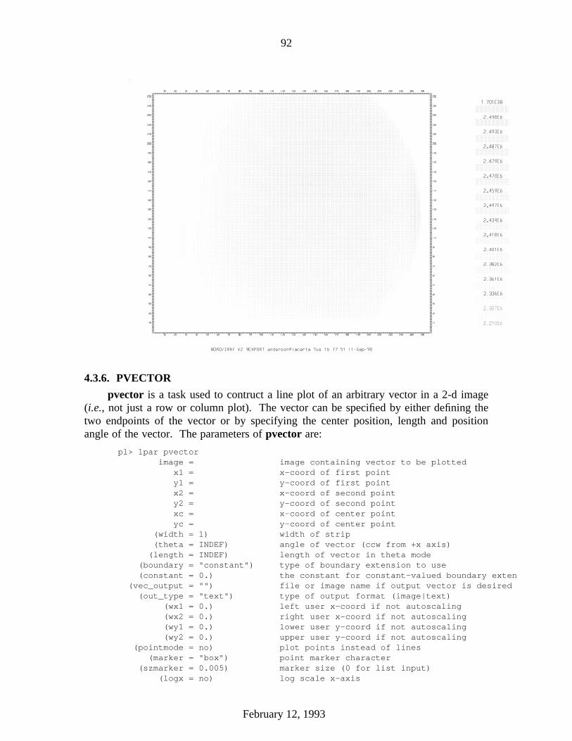
92

.

4.3.6. PVECTOR

pvector is a task used to contruct a line plot of an arbitrary vector in a 2-d image(i.e., not just a row or column plot). The vector can be specified by either defining thetwo endpoints of the vector or by specifying the center position, length and positionangle of the vector. The parameters of pvector are:

pl> lpar pvectorimage = image containing vector to be plotted

x1 = x-coord of first pointy1 = y-coord of first pointx2 = x-coord of second pointy2 = y-coord of second pointxc = x-coord of center pointyc = y-coord of center point

(width = 1) width of strip(theta = INDEF) angle of vector (ccw from +x axis)(length = INDEF) length of vector in theta mode

(boundary = "constant") type of boundary extension to use(constant = 0.) the constant for constant-valued boundary exten

(vec_output = "") file or image name if output vector is desired(out_type = "text") type of output format (image|text)

(wx1 = 0.) left user x-coord if not autoscaling(wx2 = 0.) right user x-coord if not autoscaling(wy1 = 0.) lower user y-coord if not autoscaling(wy2 = 0.) upper user y-coord if not autoscaling

(pointmode = no) plot points instead of lines(marker = "box") point marker character

(szmarker = 0.005) marker size (0 for list input)(logx = no) log scale x-axis

February 12, 1993

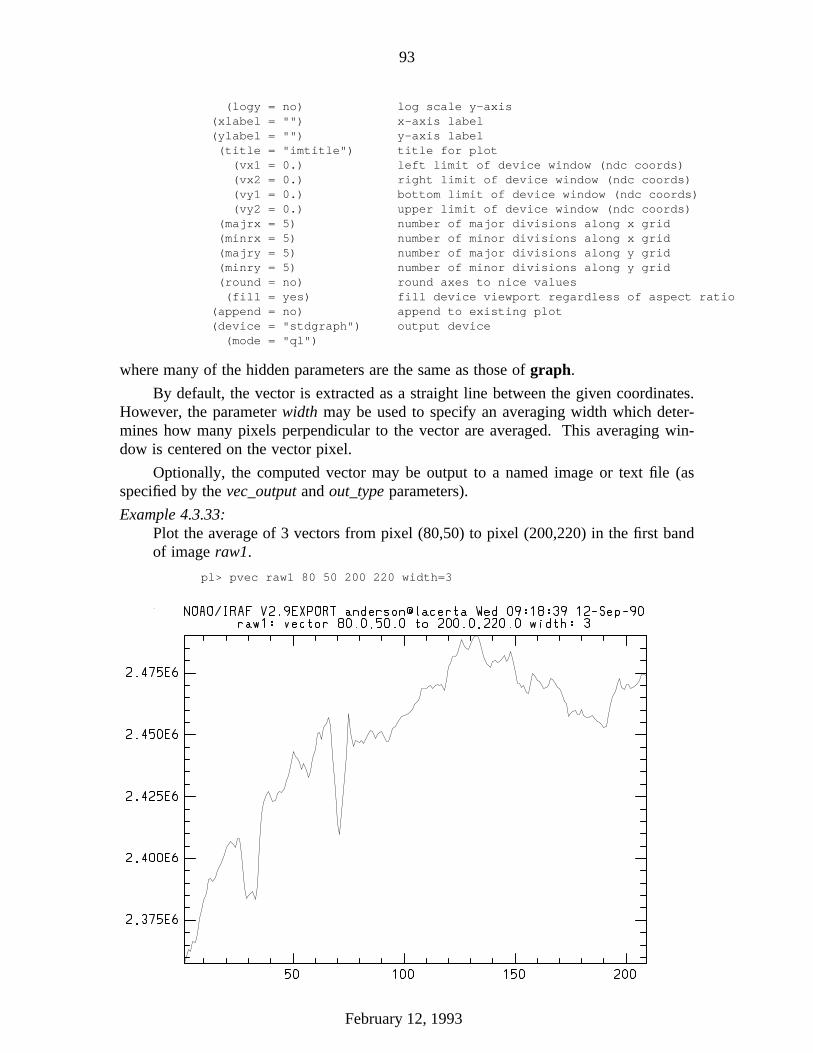
93

(logy = no) log scale y-axis(xlabel = "") x-axis label(ylabel = "") y-axis label(title = "imtitle") title for plot

(vx1 = 0.) left limit of device window (ndc coords)(vx2 = 0.) right limit of device window (ndc coords)(vy1 = 0.) bottom limit of device window (ndc coords)(vy2 = 0.) upper limit of device window (ndc coords)

(majrx = 5) number of major divisions along x grid(minrx = 5) number of minor divisions along x grid(majry = 5) number of major divisions along y grid(minry = 5) number of minor divisions along y grid(round = no) round axes to nice values(fill = yes) fill device viewport regardless of aspect ratio

(append = no) append to existing plot(device = "stdgraph") output device(mode = "ql")

where many of the hidden parameters are the same as those of graph.

By default, the vector is extracted as a straight line between the given coordinates.However, the parameter width may be used to specify an averaging width which deter-mines how many pixels perpendicular to the vector are averaged. This averaging win-dow is centered on the vector pixel.

Optionally, the computed vector may be output to a named image or text file (asspecified by the vec_output and out_type parameters).

Example 4.3.33:Plot the average of 3 vectors from pixel (80,50) to pixel (200,220) in the first bandof image raw1.

pl> pvec raw1 80 50 200 220 width=3

.

February 12, 1993

94

Example 4.3.34:Save the vector of the above example as a new image called raw1_vec.

pl> pvec raw1 80 50 200 220 width=3 vec_out=raw1_vec out_type=image

4.3.7. VELVECT

velvect draws a representation of a two-dimensional velocity field by drawingarrows from each data location where the length of the arrow is proportional to thestrength of the field and the direction of the arrow indicates the direction of the flow.

pr> lpar velvectu_image = image or image section to be plottedv_image = image or image section to be plotted(device = "stdgraph") output device(title = "imtitle") optional title(append = no) append to an old plot(verbose = yes) print warning messages

(mode = "ql")

The two images uimage and vimage contain the vector field components. The vec-tor at the point (i,j) has:

magnitude = √uimagei, j2 + vimagei, j

2 direction = tan−1î uimagei, j

vimagei, j

Example 4.3.35:The following is the vector field produced from two bands of a dark correctedGONG calibration image. The dark image used for the correction was defectiveand resulted in the broad low magnitude feature shown in this plot.

pl> velvec c082357[*:8,*:8,1] c082357[*:8,*:8,2]

.

February 12, 1993

95

4.3.8. Cursor Mode

Many IRAF tasks (not just those in the plot package) produce a plot of some sortand then bring up a graphics cursor (e.g., a crosshair) and automatically leave the termi-nal in cursor mode. Alternatively, the user can invoke cursor mode from the CL bytyping

cl> = gcur

While in cursor mode, help text may be obtained in at least two ways. Help onthe cursor mode commands themselves is available with the command

:.help

or just

:.

By convention help on an application task running cursor mode (e.g., implot) is avail-able with the command ?. All interactive IRAF graphics tasks are required to respondto the ? key with a summary of the keystrokes recognized by that task.

While in cursor mode, whether invoked by an IRAF task or interactively via thecommand =gcur, three classes of commands are available.

1) Single, upper-case letters take actions such as roaming and zooming, redraw-ing axes after a zoom, and prompting for text annotation. These commandsare:

A - draw and label the axes of current viewportB - backup over last instruction in frame bufferC - print the cursor position as it movesD - draw a line by marking the endpointsE - expand plot by setting window cornersF - set fast cursor (for HJKL)H - step cursor leftJ - step cursor downK - step cursor upL - step cursor rightM - move point under cursor to center of screenP - zoom out (restore previous expansion)R - redraw the screenT - draw a text stringU - undo last frame buffer editV - set slow cursor (for HJKL)W - select WCS at current position of cursorX - zoom in, X onlyY - zoom in, Y onlyZ - zoom in, both X and Y< - set lower limit of plot to the cursor y value> - set upper limit of plot to the cursor y value\ - escape next character: - set cursor mode options:! - send a command to the host system= - short for ":.snap"0 - reset and redraw1-9 - roam

February 12, 1993

96

2) Cursor-mode options and more complicated commands may be entered aftera :., for example sending a screen snapshot to a hardcopy plotter and chang-ing text quality and orientation. These commands are:

:.axes[+-] draw axes of viewport whenever screen is redrawn:.case[+-] enable case sensitivity for keystrokes:.clear clear alpha memory (e.g, this text):.cursor n select cursor (0=normal,1=crosshair,2=lightpen):.gflush flush plotter output:.help print help text for cursor mode:.init initialize the graphics system:.markcur[+-] mark cursor position after each cursor read:.off [keys] disable selected cursor mode keys:.on [keys] enable selected cursor mode keys:.page[+-] enable screen clear before printing help text:.read file fill frame buffer from a file:.show print cursor mode and graphics kernel status:.snap [device] make hardcopy of graphics display:.txqual qual set character generator quality (normal,l,m,h):.txset format set text drawing parameters (size,up,hj,vj,etc):.xres=value set X resolution (stdgraph only):.yres=value set Y resolution (stdgraph only):.viewport x1 x2 y1 y2 set workstation viewport in world coordinates:.write[!][+] file save frame buffer in a spool file:.zero reset viewport and redraw frame

3) All other commands, namely the lower case letters and most nonal-phanumeric characters, are interpreted by the controlling task (e.g., implot).

Minimum match abbreviations are permitted for the cursor mode :. command names.Multiple commands may be given on one line, delimited by semicolons.

The following items are brief notes about some of the features of cursor mode.Detailed information is available from the cursors help page.

The Frame BufferIRAF tasks output all graphics in the form of GKI metacode instructions. Theseinstructions may be stored in a file if desired, or, if the task is run from the CL,they will usually be stored automatically in the frame buffer. What is important isthat after producing a plot on the screen, all or part of the information in the plotis still present in the frame buffer. That means that it is possible to enter aninteractive session with the plot, whether as a part of the task that produced theplot in the first place or after the task exits by typing =gcur from the CL.

If one wishes to recall the last plot after the task which created it has exited, andthe screen has since been cleared (as opposed to the plot frame being erased) theplot will still be in the frame buffer and can be redrawn by entering cursor modeand typing 0 (the digit zero).

Frame Buffer SizeAll graphics instructions output since the last time the device screen was clearedreside in the frame buffer unless there is an extremely large amount of informationin the plot, in which case only the last part of the plot will be saved (the frame

February 12, 1993

97

buffer dynamically sizes itself to fit the frame, but there is a fixed upper limit onits size of about 100 Kb).

If one is doing complex plots (e.g, contour, hafton, velvect) or plotting anextremely large number of points, then to be sure that the frame buffer is largeenough, one may want to reset the maximum size via the following commands:

cl> set cmbuflen = 256000cl> gflush

It may be wise to put these commands in the loginuser.cl file.

Writing and Reading the Frame BufferThe contents of the frame buffer may be written to a metacode file with :.writefile. By default the frame buffer is appended to the file if it already exists. If youwish to clobber (i.e., overwrite) an existing file, use :.write! file. Also by default,the frame that is written is what you currently see on the screen (i.e., if you havezoomed in on a feature only what you see on the screen will be saved). To writethe full frame (the one you would see if you first did a 0), use :.write+ file. Tooverwrite an existing metacode file in full-frame mode, use :.write!+ file.

To read a metacode file into the current frame buffer, use the command :.read file.

Moving the Cursor and Modifying the PlotAs can be seen from the above lists, a number of special keystrokes are recognizedfor interactive display control. These keystrokes may be used to redraw all or anyportion of the spooled graphics (e.g., one may zoom in on a portion of the plot andthen roam about on the plot at high magnification). Since the spooled graphicsvectors often contain more information than can be displayed at normalmagnification (e.g., a GONG power spectrum), zooming in on a feature may bringout additional detail (the maximum resolution is 32768 points in either axis).Increasing the magnification will increase the precision of a cursor read by thesame factor.

� Magnifying a portion of the plot may cause the axes to be lost. One may usethe A keystroke to draw and label the axes of the displayed window.

� The command :.axes+ will cause new axes to be drawn every time theviewport changes.

� The commands H, J, K, and L move the cursor left, down, up, and right.

F increases the step size by a factor over the current step size each time it isused; V decreases it similarly. In practice these speed keys are rarely usedbecause the cursor positioning algorithm will automatically adjust the stepsize as you move the cursor. A large step size is used to cross the screen,then the step size is automatically decreased (by jumping the cursor in theopposite direction) as you get close to the desired feature. Some practice isrequired to become adept at this, but soon it becomes natural and fast (ofcourse, on workstations it is much faster to use the mouse).

February 12, 1993

98

� The numeric keypad of the terminal (if it has one) may be used to roam aboutwhen the zoom factor is greater than one. The directional significance of thenumeric keys in roam mode is obvious if the terminal has a keypad, and isillustrated below.

KEYPAD DIRECTION(degrees)

7 8 9 135 090 045

4 5 6 180 000 000

1 2 3 -135 -90 -45

If the keypad does not work, the normal numeric keys at the top of the key-board will.

� The command C is a toggle that causes the world (data) coordinates of thecursor to be reported. Every time the cursor is moved with HJKL, the worldcoordinates at each new position will be reported on the lower left line of thescreen.

If the cursor is moved some other way the world coordinates are not automat-ically read out. In this case one may have to use the C command twice toturn the readout off and back on again in order to get the new position.

� Some plots have more than one world coordinate system. Suppose you are incursor mode and the frame contains two separate plots, or there is only oneplot but the lower x-axis is in Angstroms while the upper one is in inversecentimeters. By default the graphics system will automatically select theWCS (viewport) closest to the position of the cursor, returning a cursor posi-tion in that coordinate system. If this is not what is desired, move the cursorto a position that belongs unambiguously to one of the coordinate systemsand type W. Subsequent cursor reads will refer to the coordinate system youhave specified, regardless of the position of the cursor on the screen. Whenthe frame is cleared the WCS lock will be cleared as well.

Annotating PlotsTo annotate a plot, position the cursor where the text string is to appear and hit T.You will then be prompted for the text string. The text will appear on the screen(and get stored in the frame buffer), normally located with its lower left corner atthe current cursor position. This command may be used in conjunction with the Dcommand to draw a line from the text annotation to a feature of interest in theplot.

The text size is constant in cursor mode regardless of the current magnification. Inorder that text entered with T will look as nearly the same as possible on a hard-copy snapshot as it does on the screen, you should set text quality to high.

February 12, 1993

99

The text attributes are controlled by two command options:

:.txqual optionThis command sets the quality of the text. The options are normal (thedefault), low, medium, and high.

:.txset optionThis command allows the user to set various options regarding size, orienta-tion, direction and quality of the annotation text. The options are:

Keyword Possible Values Default

up degrees counterclockwise, zero = +x 90size character size scale factor 1.0path left, right, up, down righthjustify normal, center, left, right leftvjustify normal, center, top, bottom bottomfont roman, greek, italic, bold romanquality normal, low, medium, high normalcolor integers greater than one 1

The up keyword controls the orientation of the character and the whole textstring. For example, a text string oriented at +45 degrees to the horizontal,from left to right, would have:

:.txset up=135

Character sizes are all specified relative to a base size characteristic of eachplotting device. The size is a linear magnification factor.

The path is relative to the up vector; a string of characters consecutivelyunderneath each other with the normal upright orientation would have:

:.txset up=90; path=down

The justify parameters refer to the placement of the entire text string relativeto the current cursor position. For example, to center a text string horizon-tally over a spike in a plot, with the cursor positioned just above the spike,one would use the command:

:.txset h=c;v=b

Example 4.3.36:This is the same as Example 4.3.1 (implot raw1), but this plot has been annotated.The keystroke sequence is listed below:

:l 173:x 30 70:y 2.0e6 2.5e6:i raw1[*,*,2]o:l 173:i raw1[*,*,3]

February 12, 1993

100

o:l 173:.txqual hiT [after positioning Cursor, type "Band 1"]T [after positioning Cursor, type "Band 2"]T [after positioning Cursor, type "Band 3"]D [draw line from "Band 1" to solid line plot]DD [draw line from "Band 2" to dashed line plot]DD [draw line from "Band 3" to dotted line plot]D

.

Other Items of Note� The B command is used to back up over the last instruction and redraw (e.g.

with 0) until you’re ready to reenter the text. If you back up one instructiontoo far (you lose some of the data vectors for instance) just type U to undothe last frame buffer edit (i.e. the backup).

� The :.clear command is useful on VT100 and Retrographics type terminalsfor wiping away foreground (i.e., Alpha-mode) text from a plot.

� The M and/or the :.viewport commands are handy for combining more thanone plot into a given viewport.

Example 4.3.37:The following plot (from the Longslit demonstration) was created by saving eachof the individual plots to a file and then reading them back into different spots inthe graphics window.

February 12, 1993

101

.

4.3.9. Hardcopy Output

There are two main ways to get a hardcopy of the frame buffer:

1) To get a copy of what you see on the screen directly on a hardcopy plotter, use acursor command of the form

:.snap plotter_device_name.

where the default device is STDPLOT.

Note that when making hardcopies in this fashion the output is being buffered.That is, you can do several :.snap’s before anything actually comes out on theplotter. If planning to make a number of snapshots in succession, even if they arefrom different =gcur or interactive plotting sessions use :.snap for each one untildone and then issue the command to flush the graphics output buffer. From cursormode the command is:

:.gflush

or from the cl:

cl> gflush

2) Alternatively one may first write a metacode file (:.write mcodefile) and then sendthe metacode to the desired plotter using one of the graphics kernels (e.g., stdplot,imdkern or gkimosaic).

February 12, 1993

102

4.3.10. Alternate Cursor Input

The task implot and many of the IRAF applications tasks that use interactivegraphics have a hidden parameter usually called cursor or coords, which defaults tointeractive cursor input. However, these tasks may be run in batch mode with the cur-sor parameter set to the name of a file containing the cursor intructions.

The cursor file is a text file where every line is a cursor command of the form

x y world_coord_sys command [colon_command_string]

where

x, y - The cursor position in world coordinates.world_coord_sys - The number of the world coordinate system.

(This is almost always 1)command - The cursor command to be executed.

colon_command_string - The string to follow a ‘:’ in the command field.

Note: A current limitation is that cursor mode keystrokes (capital letters and :. com-mands) cannot be used, since the cursor file replaces the cursor mode interac-tion.

Example 4.3.38:To construct overlay plots of the central row and column of the first band in aseries of GONG raw data images, the following cursor file (called say,implot.cur) would be used,

1 1 1 : "l 128"1 1 1 o1 1 1 : "c 128"

Note, it is not necessary to include the q command in the cursor file, as theEOF of the file acts as the q command.

To execute the above on the raw data, one would use a command of the form

pl> files raw*.imh > raw.listpl> list = "raw.list"pl> while (fscan(list,s1) != EOF)>>> implot @raw.list coord="implot.cur" >>G "implot.plt"

where the G token has been used to redirect the graphics output to a metacodefile (implot.plt). The metacode file could then be viewed with gkimosaic orstdgraph, or sent to the plotter.

Note: This particular example produced two plots for every input image(one being a plot of row 128, the other being the desired overplot ofrow and column 128). The task gkiextract could be used to get theoverplots only out of the metacode file.

Note: The list and while-loop are used to input data to implot becauseimplot only works on one file at a time.

February 12, 1993

103

4.3.11. The Graphics Kernel Tasks

The graphics kernel tasks are used to dispose metacode files to various terminal orhardcopy output devices.

stdgraphDraws the plot(s) on the standard terminal device.

pl> lpar stdgraphinput = input metacode file

(device = "stdgraph") output device(generic = no) ignore remaining kernel dependent parameters(debug = no) print decoded graphics instructions during proc

(verbose = no) print elements of polylines, cell arrays, etc.(gkiunits = no) print coordinates in GKI rather than NDC units

(txquality = "normal") character generator quality(xres = 0) number of points of resolution in x(yres = 0) number of points of resolution in y(mode = "ql")

The parameters txquality, xres, and yres are used to override the values for textquality, and x and y resolution already in the metacode. The other parameters areused mainly for debugging purposes.

stdplotDraws the plot(s) on the standard plotter device.

pl> lpar stdplotinput = input metacode file

(device = "stdplot") output device(generic = no) ignore remaining kernel dependent parameters(debug = no) print decoded graphics instructions during proc

(verbose = no) print elements of polylines, cell arrays, etc.(gkiunits = no) print coordinates in GKI rather than NDC units

(mode = "ql")

The output device may be any hardcopy device known to IRAF (e.g., lw1). Theother parameters are used mainly for debugging purposes.

gkidirPrints a directory of plots within the named metacode file.

pl> lpar gkidirinput = "" Metacode file(mode = "ql")

Each plot is listed with its size and an identifying title string. The output format isshown in the following example:

pl> gkidir file1,file2METAFILE ’file1’:

[1] (1234 words) title_string[2] (78364 words) title_string

METAFILE ’file2’:[1] (874 words) title_string

February 12, 1993

104

The title string may be some string written by the plot task that created themetafile (not used by any IRAF tasks at this point), or else the longest text stringfound (hopefully the plot title), or else the string "no title)".

gkiextractgkiextract extracts specified frames from a GKI metacode file and outputs them toSTDOUT.

pl> lpar gkiextractinput = "" metacode source fileframes = "1-99" ranges of frames to extract

go_ahead = yes ?(verify = no) verify operation before extracting each frame?

(default_acti = yes) default extract action for verify query(mode = "ql")

Example 4.3.39:Extract files 2,4 and 8 from the metacode file, implot.plt, and output to annew file, implot.select.

pl> gkiextract implot.plt 2,4,8 >> implot.select

Example 4.3.40:Extract files 2,4 and 8 from the metacode file, implot.plt, and output directlyto the versatec plotter.

pl> gkiextract implot.plt 2,4,8 | stdplot dev=versatec

gkimosaicgkimosaic condenses the plots in a metacode file to fit on a single page. The plotscan be examined interactively after each pageful. The number of plots in x and ycan be specified. This task is extremely useful for browsing through a largemetacode file, and for compactly plotting a large number of metacode frames.

pl> lpar gkimosaicinput = "" metacode input

(device = "stdgraph") output device(output = "") name of binary output file

(nx = 2) number of plots in x direction(ny = 2) number of plots in y direction

(rotate = no) rotate axes?(fill = no) fill viewport vs preserve aspect ratio

(interactive = yes)(cursor = "")

(mode = "ql")

The mosaiced plots are drawn on the page rotated by 90 degrees when rotate =yes. This means the x axis of the plots can be placed along either the page widthor length.

The plots can be output to a plotting device, or spooled in metacode file output forlater plotting.

February 12, 1993

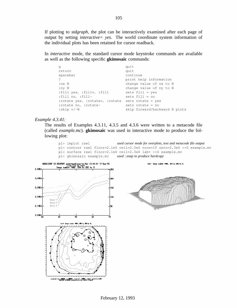
105

If plotting to stdgraph, the plot can be interactively examined after each page ofoutput by setting interactive= yes. The world coordinate system information ofthe individual plots has been retained for cursor readback.

In interactive mode, the standard cursor mode keystroke commands are availableas well as the following specific gkimosaic commands:

q quitreturn quitspacebar continue? print help information:nx N change value of nx to N:ny N change value of ny to N:fill yes, :fill+, :fill sets fill = yes:fill no, :fill- sets fill = no:rotate yes, :rotate+, :rotate sets rotate = yes:rotate no, :rotate- sets rotate = no:skip +/-N skip forward/backward N plots

Example 4.3.41:The results of Examples 4.3.11, 4.3.5 and 4.3.6 were written to a metacode file(called example.mc). gkimosaic was used in interactive mode to produce the fol-lowing plot:

pl> implot raw1 used cursor mode for overplots, text and metacode file outputpl> contour raw1 floor=2.1e6 ceil=2.5e6 ncon=10 zero=2.3e6 >>G example.mcpl> surface raw1 floor=2.1e6 ceil=2.5e6 lab+ >>G example.mcpl> gkimosaic example.mc used :.snap to produce hardcopy

.

February 12, 1993

106

4.3.12. Graphics Overlays on the Image Display (IMDKERN)

There are times when one might wish to overlay graphics in the image display.Typically the overlay is a contour plot. The task imdkern is used to draw graphicsinto the image display. One first displays the image, then runs imdkern to overlay thegraphics on the displayed image. The parameters are as follows:

pl> lpar imdkerninput = "contour.mc" input metacode file

(device = "stdimage") output device(generic = no) ignore remaining kernel dependent parameters(frame = 0) display frame(color = 205) color index(debug = no) print decoded graphics instructions during proc

(verbose = no) print elements of polylines, cell arrays, etc.(gkiunits = no) print coordinates in GKI rather than NDC units

(mode = "ql")

For IMTOOL and compatible display servers (e.g., SAOIMAGE) the possiblecolor values that may be used are

202 - black 203 - white204 - red 205 - green206 - blue 207 - yellow208 - cyan 209 - magenta210 - coral 211 - maroon212 - orange 213 - khaki214 - orchid 215 - turquoise216 - violet 217 - wheat

imdkern always overlays a plot on whatever is currently in the display framebuffer. Thus to erase the graphics drawn by imdkern, one must redisplay the frameusing display or a similar program, or erase the frame entirely.

imdkern may be called either explicitly as a task, to plot a graphics metacode file,or implicitly when the output of a graphics task is directed to a device which uses theIMD kernel. The standard IRAF graphcap file defines the following logical IMDgraphics devices:

imd|imdkern same as imdgimdw output to stdimage, frame=0, color=whiteimdr output to stdimage, frame=0, color=redimdg output to stdimage, frame=0, color=greenimdb output to stdimage, frame=0, color=blueimdy output to stdimage, frame=0, color=yellow

where the frame=0 parameter causes the graph to be plotted in the currently displayedimage display frame.

Example 4.3.42:Capture the output of contour in a metacode file and overlay in the display frame2 (in red).

pl> contour raw1 floor=2.1e6 ceil=2.5e6 ncon=10 zero=2.3e6 \\>>> xres=128 yres=128 perim- fill+ >G contour.mcpl> imdkern contour.ms color=204 frame=2

February 12, 1993

107

Example 4.3.43:Same as above, except have contour do the overlay directly.

pl> contour raw1 floor=2.1e6 ceil=2.5e6 ncon=10 zero=2.3e6 \\>>> xres=128 yres=128 perim- fill+ dev=imdr

Note: It has been the authors limited experience that square images must bedisplayed with fill=yes, and likewise the contour plot must also have fill+ aswell as perimeter=no in order to correctly line up the overlay.

Rectangular images are more of a problem. For these images, one may haveto play with the display magnification factors and centering, and/or the con-tour viewport coordinates.

Also note that a higher than normal resolution contour plot is generated toavoid the contour placement errors that occur when a large block-averagingfactor is used to generate the contour map (this can make contours drawnaround objects such as stars appear to not be centered on the object).

The following is screendump showing the contour plot of Example 4.3.5, overlayed ona display of the image raw1..

February 12, 1993

108

4.4. Image Manipulation (IMAGES)

The IMAGES package contains tasks to perform a wide variety of functions: filter-ing, edge detection, mosaicing, arithmetic, geometric transforms, etc. The following isthe help menu for the IMAGES package (IRAF Version 2.9):

images.:blkavg - Block average or sum a list of N-D imagesblkrep - Block replicate a list of imagesboxcar - Boxcar smooth a list of 1 or 2-D images

chpixtype - Change the pixel type of a list of imagesconvolve - Convolve a list of 1 or 2-D images with a rectangular filter

fit1d - Fit a function to image lines or columnsfmedian - Quantize and median filter a 2-D image or a list of imagesfmode - Quantize and modal filter a 2-D image or list of imagesgauss - Convolve a list of 1 or 2-D images with an elliptical Gaussian

geomap - Calculate a coordinate transformationgeotran - Geometrically transform a set of 2-D images

gradient - Convolve a list of 1 or 2-D images with a gradient operatorhedit - Header editor

hselect - Select a subset of images satisfying a boolean expressionimarith - Simple image arithmetic

imcombine - Combine images pixel-by-pixel using various algorithmsimcopy - Copy an imageimdebug - Image debugging package (currently undocumented)imdelete - Delete a list of imagesimdivide - Image division with zero checking and rescaling

imgets - Return the value of an image parameter as a stringimheader - Print an image header

imhistogram - Compute image histogramimlintran - Linearly transform a list of 2-D imagesimrename - Rename one or more imagesimshift - Shift a list of 2-D imagesimslice - Slice images into images of lower dimensionimstack - Stack images into a single image of higher dimension

imstatistics - Compute and print statistics for a list of imagesimsum - Compute the sum, average, or median of a set of images

imsurfit - Fit a surface to a 2-D imageimtranspose - Transpose a 2-D image

laplace - Laplacian filter a list of 1 or 2-D imageslineclean - Replace deviant pixels in image lineslistpixels - Convert an image section into a list of pixels

magnify - Magnify a list of 1-D or 2-D imagesmedian - Median filter a 2-D image or list of imagesminmax - Compute the minimum and maximum pixel values in an image

mode - Modal filter a 2-D image or list of imagesregister - Register a set of imagesrotate - Rotate and shift a list of 2-D images

sections - Expand an image template on the standard outputshiftlines - Shift image lines

tv - Image display load and control package

The following sections very briefly descibe the various classes of image operationsthat can be performed with these tasks.

February 12, 1993

109

4.4.1. Image Section Notation

All IRAF programs which operate upon images may be used to operate on theentire image (the default) or any section of the image. A special notation is used tospecify image sections. The section notation is appended to the file name of the image,much like an array subscript is appended to an array name in a conventional program-ming language. If no section is specified, the entire image will be used.

Section Refers to

pix[] whole image

pix[i,j] the pixel value (scalar) at [i,j]

pix[*,*] whole image, two dimensions

pix[*,−*] flip y-axis

pix[*,*,b] band B of three dimensional image

pix[*,*:s] subsample in y by S

pix[*,l] line L of image

pix[c,*] column C of image

pix[x1:x2,y1:y2] subraster of image

pix[x1:x2:sx,y1:y2:sy] subraster with subsampling

A limited class of coordinate transformations may be specified using image sec-tions (but transpose is not one of them). The "match all" (asterisk), flip, subsample,index, and range notations shown in the table may be combined just about any way thatmakes sense. Some examples have already appeared in the text.

Example 4.4.44:As a simple example, the following command will graph line 10 of the imagemyimage:

cl> graph myimage[*,10]

Example 4.4.45:To generate a contour plot of an 800 pixel square, two-dimensional image on thegraphics terminal, subsampling by a factor of 16 in both dimensions,

cl> contour myimage[*:16,*:16]

Example 4.4.46:To display the fifth x,z plane of the three dimensional image named cube on frame1 of the image display device,

cl> display cube[*,5,*] 1

February 12, 1993

110

4.4.2. Getting Information About an Image

There are a number of tasks which report and/or calculate and report informationabout an image.

imheaderThis task is used to print header information in various formats for a list of IRAFimages. The parameters are as follows:

im> lpar imheadimages = "raw1" image names

(longheader = no) print header in multi-line format(userfields = yes) print the user fields (instrument parameters)

(mode = "ql")

If longheader = no, the image name, dimensions, data type and title is listed.

If longheader = yes, information on the create and modify dates, image statisticsand so forth are printed.

Non-standard IRAF header information (i.e., FITS-like header keywords) can beprinted by setting longheader = yes and userfields = yes.

Example 4.4.47:To list the short headers for all GONG west limb calibration images,

im> imhead calwlm*.imhcalwlmavg.imh[256,252,2][real]: brd<<brd-darkcalwlm085222.imh[256,252,2][real]: brd<<brd-darkcalwlm104329.imh[256,252,2][real]: brd<<brd-darkcalwlm131123.imh[256,252,2][real]: brd<<brd-darkcalwlm153130.imh[256,252,2][real]: brd<<brd-darkcalwlmvm.imh[256,252,2][real]: brd<<brd-darkcalwlmavg1.imh[256,252,2][real]: brd<<brd-dark

Example 4.4.48:To list the long header for calwlmavg,

im> imhead calwlmavg l+calwlmavg[256,252,2][real]: brd<<brd-dark

No bad pixels, no histogram, min=unknown, max=unknownLine storage mode, physdim [256,252,2], length of user area 1135 s.u.Created Wed 12:16:30 07-Mar-90, Last modified Wed 12:16:30 07-Mar-90Pixel file ’serpens!/u2/roberta/data/calwlmavg.pix’ [ok]New copy of 085107.imhNew copy of d085107.imhNew copy of c085107.imhNew copy of mskcal[*,*,1]New copy of mskcal1New copy of eastvmiNew copy of eastxyNew copy of /u2/roberta/iraf/jun8/calwlm085222DTYPE = ’RW ’ / TWO CHARACTER ABBREVIATION FOR DATA TYPESITE = ’BB ’ / TWO CHARACTER ABBREVIATION FOR OBSERVING SIUT_DATE = ’89/06/08 ’ / UT DATE OF OBSERVATIONUT_TIME = ’16:05:20 ’ / UT TIME OF OBSERVATION

February 12, 1993

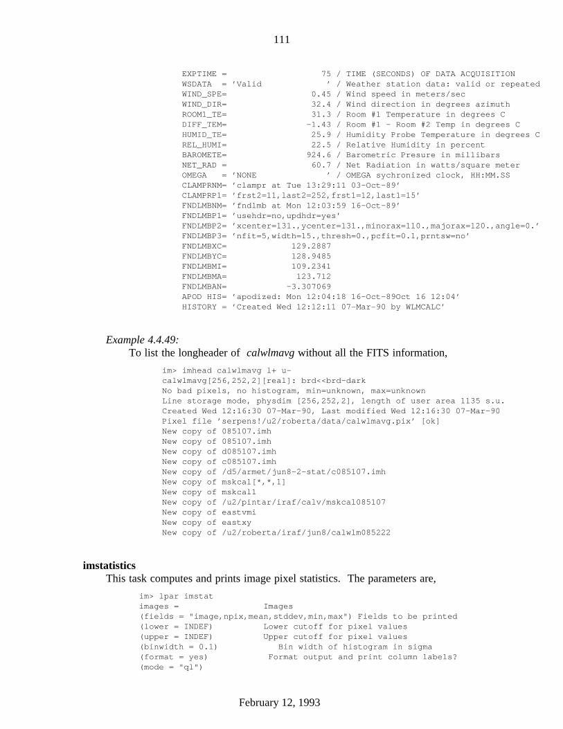
111

EXPTIME = 75 / TIME (SECONDS) OF DATA ACQUISITIONWSDATA = ’Valid ’ / Weather station data: valid or repeatedWIND_SPE= 0.45 / Wind speed in meters/secWIND_DIR= 32.4 / Wind direction in degrees azimuthROOM1_TE= 31.3 / Room #1 Temperature in degrees CDIFF_TEM= -1.43 / Room #1 - Room #2 Temp in degrees CHUMID_TE= 25.9 / Humidity Probe Temperature in degrees CREL_HUMI= 22.5 / Relative Humidity in percentBAROMETE= 924.6 / Barometric Presure in millibarsNET_RAD = 60.7 / Net Radiation in watts/square meterOMEGA = ’NONE ’ / OMEGA sychronized clock, HH:MM.SSCLAMPRNM= ’clampr at Tue 13:29:11 03-Oct-89’CLAMPRP1= ’frst2=11,last2=252,frst1=12,last1=15’FNDLMBNM= ’fndlmb at Mon 12:03:59 16-Oct-89’FNDLMBP1= ’usehdr=no,updhdr=yes’FNDLMBP2= ’xcenter=131.,ycenter=131.,minorax=110.,majorax=120.,angle=0.’FNDLMBP3= ’nfit=5,width=15.,thresh=0.,pcfit=0.1,prntsw=no’FNDLMBXC= 129.2887FNDLMBYC= 128.9485FNDLMBMI= 109.2341FNDLMBMA= 123.712FNDLMBAN= -3.307069APOD HIS= ’apodized: Mon 12:04:18 16-Oct-89Oct 16 12:04’HISTORY = ’Created Wed 12:12:11 07-Mar-90 by WLMCALC’

Example 4.4.49:To list the longheader of calwlmavg without all the FITS information,

im> imhead calwlmavg l+ u-calwlmavg[256,252,2][real]: brd<<brd-darkNo bad pixels, no histogram, min=unknown, max=unknownLine storage mode, physdim [256,252,2], length of user area 1135 s.u.Created Wed 12:16:30 07-Mar-90, Last modified Wed 12:16:30 07-Mar-90Pixel file ’serpens!/u2/roberta/data/calwlmavg.pix’ [ok]New copy of 085107.imhNew copy of 085107.imhNew copy of d085107.imhNew copy of c085107.imhNew copy of /d5/armet/jun8-2-stat/c085107.imhNew copy of mskcal[*,*,1]New copy of mskcal1New copy of /u2/pintar/iraf/calv/mskcal085107New copy of eastvmiNew copy of eastxyNew copy of /u2/roberta/iraf/jun8/calwlm085222

imstatisticsThis task computes and prints image pixel statistics. The parameters are,

im> lpar imstatimages = Images(fields = "image,npix,mean,stddev,min,max") Fields to be printed(lower = INDEF) Lower cutoff for pixel values(upper = INDEF) Upper cutoff for pixel values(binwidth = 0.1) Bin width of histogram in sigma(format = yes) Format output and print column labels?(mode = "ql")

February 12, 1993

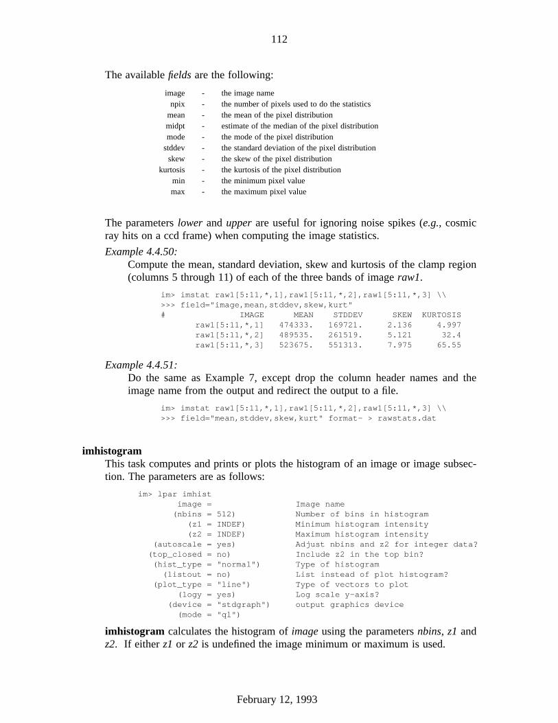
112

The available fields are the following:

image - the image namenpix - the number of pixels used to do the statistics

mean - the mean of the pixel distributionmidpt - estimate of the median of the pixel distributionmode - the mode of the pixel distribution

stddev - the standard deviation of the pixel distributionskew - the skew of the pixel distribution

kurtosis - the kurtosis of the pixel distributionmin - the minimum pixel valuemax - the maximum pixel value

The parameters lower and upper are useful for ignoring noise spikes (e.g., cosmicray hits on a ccd frame) when computing the image statistics.

Example 4.4.50:Compute the mean, standard deviation, skew and kurtosis of the clamp region(columns 5 through 11) of each of the three bands of image raw1.

im> imstat raw1[5:11,*,1],raw1[5:11,*,2],raw1[5:11,*,3] \\>>> field="image,mean,stddev,skew,kurt"# IMAGE MEAN STDDEV SKEW KURTOSIS

raw1[5:11,*,1] 474333. 169721. 2.136 4.997raw1[5:11,*,2] 489535. 261519. 5.121 32.4raw1[5:11,*,3] 523675. 551313. 7.975 65.55

Example 4.4.51:Do the same as Example 7, except drop the column header names and theimage name from the output and redirect the output to a file.

im> imstat raw1[5:11,*,1],raw1[5:11,*,2],raw1[5:11,*,3] \\>>> field="mean,stddev,skew,kurt" format- > rawstats.dat

imhistogramThis task computes and prints or plots the histogram of an image or image subsec-tion. The parameters are as follows:

im> lpar imhistimage = Image name

(nbins = 512) Number of bins in histogram(z1 = INDEF) Minimum histogram intensity(z2 = INDEF) Maximum histogram intensity

(autoscale = yes) Adjust nbins and z2 for integer data?(top_closed = no) Include z2 in the top bin?(hist_type = "normal") Type of histogram

(listout = no) List instead of plot histogram?(plot_type = "line") Type of vectors to plot

(logy = yes) Log scale y-axis?(device = "stdgraph") output graphics device(mode = "ql")

imhistogram calculates the histogram of image using the parameters nbins, z1 andz2. If either z1 or z2 is undefined the image minimum or maximum is used.

February 12, 1993

113

If listout = no, the histogram is plotted on the graphics device device in the vectormode specified by plot_type.

If listout = yes, the histogram is listed on the standard output (the list is never logscaled).

The available hist_type options are normal, cumulative, difference, andsecond_difference. The later two options are marginal (forward difference) histo-grams.

Example 4.4.52:Plot the normal histogram of the first band of the image raw1.

im> imhist raw1[*,*,1]

.

minmaxThis task computes the minimum and maximum pixel values of an image andoptionally updates the image header. The parameters are as follows:

gr> lpar minmaximages = images to be examined(force = no) force recomputation of extreme values(update = yes) update the image header

(verbose = yes) print computed values(minval = ) minimum pixel value in image (output)(maxval = ) maximum pixel value in image (output)(minpix = ) minimum pixel (section notation)(maxpix = ) Maximum pixel (section notation)

(mode = "ql")

February 12, 1993

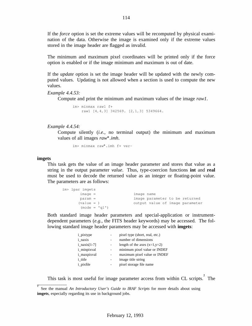
114

If the force option is set the extreme values will be recomputed by physical exami-nation of the data. Otherwise the image is examined only if the extreme valuesstored in the image header are flagged as invalid.

The minimum and maximum pixel coordinates will be printed only if the forceoption is enabled or if the image minimum and maximum is out of date.

If the update option is set the image header will be updated with the newly com-puted values. Updating is not allowed when a section is used to compute the newvalues.

Example 4.4.53:Compute and print the minimum and maximum values of the image raw1.

im> minmax raw1 f+raw1 [4,4,3] 342569. [2,1,3] 5349664.

Example 4.4.54:Compute silently (i.e., no terminal output) the minimum and maximumvalues of all images raw∗ .imh.

im> minmax raw∗ .imh f+ ver-

imgetsThis task gets the value of an image header parameter and stores that value as astring in the output parameter value. Thus, type-coercion functions int and realmust be used to decode the returned value as an integer or floating-point value.The parameters are as follows:

im> lpar imgetsimage = image nameparam = image parameter to be returned(value = ) output value of image parameter(mode = "ql")

Both standard image header parameters and special-application or instrument-dependent parameters (e.g., the FITS header keywords) may be accessed. The fol-lowing standard image header parameters may be accessed with imgets:

i_pixtype - pixel type (short, real, etc.)i_naxis - number of dimensionsi_naxis[1-7] - length of the axes (x=1,y=2)i_minpixval - minimum pixel value or INDEFi_maxpixval - maximum pixel value or INDEFi_title - image title stringi_pixfile - pixel storage file name

This task is most useful for image parameter access from within CL scripts.† The

† See the manual An Introductory User’s Guide to IRAF Scripts for more details about usingimgets, especially regarding its use in background jobs.

February 12, 1993

115

task imheader is more useful for just looking at the image header parameters.

Example 4.4.55:Get the value of the field UT_TIME from the image raw1 and put it into theCL variable x.

gr> imgets raw1 UT_TIMEgr> =imgets.value15:22:23gr> x = real(imgets.value)gr> =x15.373055555556

Notice that IRAF knows how to deal with sexegesimal notation.

heditThis task is used to modify and inspect the fields of an image header. The param-eters are as follows:

im> lpar heditimages = images to be editedfields = fields to be editedvalue = value expression(add = no) add rather than edit fields

(delete = no) delete rather than edit fields(verify = yes) verify each edit operation(show = yes) print record of each edit operation

(update = yes) enable updating of the image header(mode = "ql")

Both the standard (i.e., IRAF) and user (i.e., FITS) fields may be edited in thesame fashion, although not all standard fields are writable.

If verify mode is selected the editor will print the old value of the field and querywith the new value, allowing some other value to be entered instead. For exam-ple,

cl> hedit raw1 title "dark subtracted calibration"raw1,i_title ("clamp corrected calibration" -> "dark subtracted calibration"):

To accept the new value shown to the right of the arrow, hit RETURN or answerwith a yes or y. To continue without changing the value of the field in questionenter no or n. To enter some other value merely type in the new value.

If verification is enabled you will also be asked if you want to update the header,once all header fields have been edited. This is your last chance to change yourmind before the header is modified on disk. If you respond negatively the imageheader will not be updated, and editing will continue with the next image. If theresponse is q the editor will exit entirely.

The header editor is capable of performing global edits on entire image databaseswherein the new value of each field is computed automatically at edit time andmay depend on the values of other fields in the image header. Editing may be per-formed in either batch or interactive mode. An audit trail may be maintained (via

February 12, 1993

116

the show switch and i/o redirection), permitting restoration of the database in theevent of an error. Trial runs may be made with updating disabled, before commit-ing to an actual edit that modifies the database.

The value parameter is a string-type parameter. If the first character in the stringis a left parenthesis the string is interpreted as an algebraic expression wherein theoperands may be constants, image header variables (field names), special variables(defined below), or calls to intrinsic functions. The expression syntax isequivalent to that used in the CL and SPP languages. If the value string is notparenthesized it is assumed to be a string constant. The value string will oftencontain blanks, quotes, parenthesis, etc., and hence must usually be quoted toavoid interpretation by the CL rather than by the header editor.

The major editing functions of the hedit task are the following:

update - modify the value of a field or fieldsadd - add a new field (or modify an old one)delete - delete a set of fields

The following are a few simple examples of using hedit. The reader isencouraged to study the help pages for this task to learn how to use the advancedfeatures.

Example 4.4.56:Image raw2 has been determined to be a bad image. Edit the title appendingthe string "BAD IMAGE".

im> imhead raw2

raw1[256,252,3][real]: Image number 1883, 256 by 252 by 3.

im> hedit raw2 title "(title // ’ BAD IMAGE’)"

raw2,i_title ("Image number 1883, 256 by 252 by 3." -> "Image number 1883, 256

by 252 by 3. BAD IMAGE"):

raw2,i_title: "Image number 1883, 256 by 252 by 3." -> "Image number 1883, 256

by 252 by 3. BAD IMAGE"

update raw2 ? (yes):

raw2 updated

im> imhead raw2

raw2[256,252,3][real]: Image number 1883, 256 by 252 by 3. BAD IMAGE

Example 4.4.57:To run the above on a number of images that have been flagged as bad, onewould prepare a list (i.e., text file, one name per line) called say badlist of theimage names to be edited (see next section). The following command exe-cutes hedit silently:

im> hedit @badlist title "(title // ’ BAD IMAGE’)" ver- show-

hedit can be used to perform complex mathematical and logical operations on

February 12, 1993

117

header fields (see the help pages for details). The following operators are availablein hedit.

+ - * / arithmetic operators

** exponentiation

// string concatenation

! - boolean not, unary negation

< <= > >= order comparision (works for strings)

== != && || equals, not equals, and, or

?= string equals pattern

? : conditional expression

@ reference a variable

The conditional expression operator ?, which is patterned after a similar operatorin C, is used to make IF ELSE like decisions within an expression. The syntax isas follows:

<bool_expr> ? <true_expr> : <false_expr>

The set of intrinsic functions supported is,

abs acos asin atan atan2 bool cosexp int log log10 max min modnint real sin sqrt str tan

where the trigonometric functions operate in units of degrees.

The following special variables are recognized within expressions:

$ The value of the "current field"

$F The name of the "current field"

$I The name of the "current image"

$T The current clock time (an integer value)

These built-in variables are especially useful for constructing context-dependentexpressions. For example, the value of a field may be incremented by 100 byassigning it the the value "$ + 100".

Example 4.4.58:Go through all raw data images and add the string "HORIZON" to the title ofany image for which the zenith angle of observation (keyword zangle) isgreater than 55 degrees. Do not verify the edits, but record them in a filecalled horizon.dat.

im> hedit *.imh title ’(@"zangle" >= 45 ? (title//" Horizon") : "")’ \>>> verify- show+ >> horizon.dat

listpixelsThis task lists the pixel coordinates and values of images to STDOUT. Theparameters are as follows:

February 12, 1993

118

im> lpar listpiximages = "" Images to be converted to list form

(verbose = no) Print banner for each input image(mode = "ql")

Example 4.4.59:List the pixels for row 128 of band 2 of the image raw1 piping the output topage.

im> listpix raw[*,128,2] | page

Example 4.4.60:List the pixels for row 128 of band 2 of the image raw1 piping the output tograph in point mode.

im> listpix raw[*,128,2] | graph point+

4.4.3. Preparing Lists of Images

Most of the IRAF tasks can deal with multiple input and output files. The filescan be entered on the command line (or at the query) as a string of file names separatedby commas. For example,

im> imcopy imageA,imageB,imagec[*:2,*] outimageA,outimageB,outimageC

However, there are many times when one wants to execute a task on a very largenumber of images (or files) and entering the names on the command line becomes tedi-ous and prone to typographical error. Therefore, IRAF tasks that work on multipleinput/output will accept as their arguments files which are themselves lists ofimages/files. These files (called at files) are denoted by the character @ when given asa task parameter. For example, the above imcopy command would become

im> imcopy @inlist @outlist

where the files inlist and outlist are text files that contain the names of the respectiveimages, one name per line. Such lists can be constructed by using a text editor or byredirecting output from the SYSTEM task files, or the IMAGES tasks sections andhselect.

filesThe files command expands a file name template into a list of files sent toSTDOUT. This is a SYSTEM command and hence it is available for use immedi-ately upon login to the CL. The parameters are as follows:

im> lpar filestemplate = file template

(sort = yes) sort file list(mode = "ql")

The existence of the listed files is checked only if pattern-matching is used, hencefiles may also be used to parse a comma-delimited list of strings which are notnecessarily filenames.

February 12, 1993

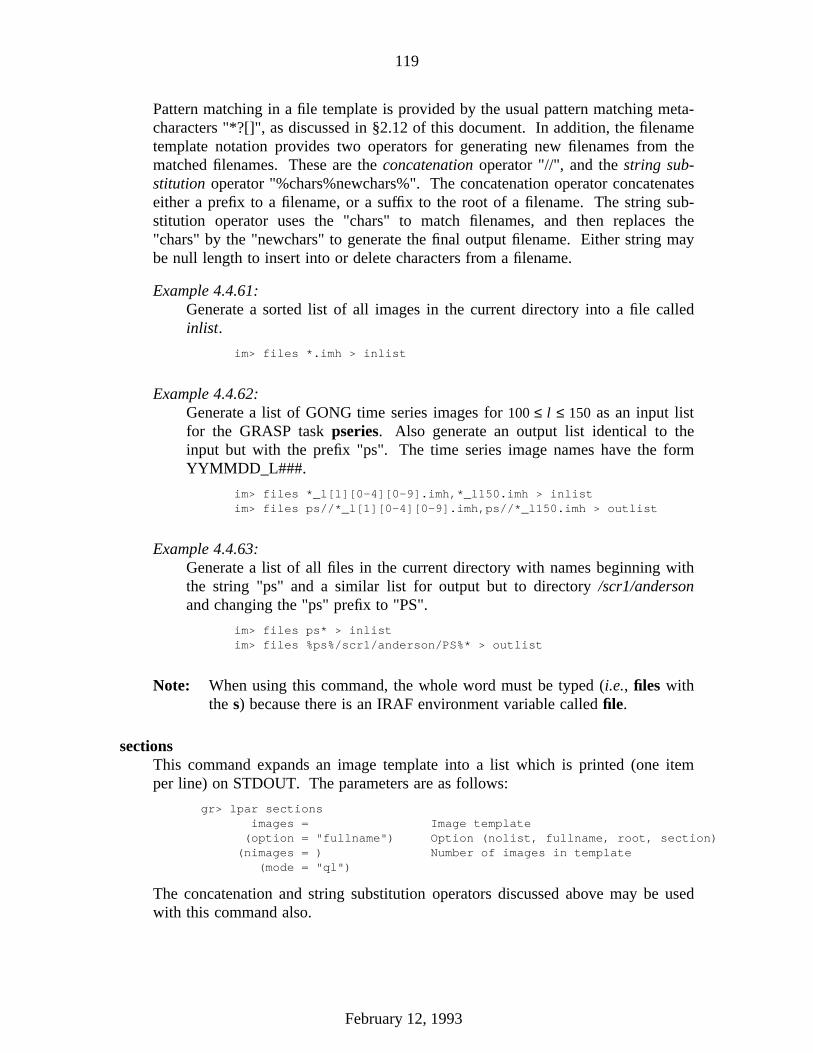
119

Pattern matching in a file template is provided by the usual pattern matching meta-characters "*?[]", as discussed in §2.12 of this document. In addition, the filenametemplate notation provides two operators for generating new filenames from thematched filenames. These are the concatenation operator "//", and the string sub-stitution operator "%chars%newchars%". The concatenation operator concatenateseither a prefix to a filename, or a suffix to the root of a filename. The string sub-stitution operator uses the "chars" to match filenames, and then replaces the"chars" by the "newchars" to generate the final output filename. Either string maybe null length to insert into or delete characters from a filename.

Example 4.4.61:Generate a sorted list of all images in the current directory into a file calledinlist.

im> files *.imh > inlist

Example 4.4.62:Generate a list of GONG time series images for 100 ≤ l ≤ 150 as an input listfor the GRASP task pseries. Also generate an output list identical to theinput but with the prefix "ps". The time series image names have the formYYMMDD_L###.

im> files *_l[1][0-4][0-9].imh,*_l150.imh > inlistim> files ps//*_l[1][0-4][0-9].imh,ps//*_l150.imh > outlist

Example 4.4.63:Generate a list of all files in the current directory with names beginning withthe string "ps" and a similar list for output but to directory /scr1/andersonand changing the "ps" prefix to "PS".

im> files ps* > inlistim> files %ps%/scr1/anderson/PS%* > outlist

Note: When using this command, the whole word must be typed (i.e., files withthe s) because there is an IRAF environment variable called file.

sectionsThis command expands an image template into a list which is printed (one itemper line) on STDOUT. The parameters are as follows:

gr> lpar sectionsimages = Image template

(option = "fullname") Option (nolist, fullname, root, section)(nimages = ) Number of images in template

(mode = "ql")

The concatenation and string substitution operators discussed above may be usedwith this command also.

February 12, 1993

120

This task is used for several purposes:

a) To verify that an image template is expanded as the user desires.

b) To create a file of image names which include image sections.

c) To create a file of new image names using the concatention feature of theimage templates.

d) To determine the number of images specified by the user in a commandlanguage script.

Example 4.4.64:Calculate and print the number of power spectrum images in the currentdirectory.

im> sections ps*.imh opt=noim> = sections.nimagesim> 251

Example 4.4.65:Copy the velocity, modulation, and intensity images of GONG VMI imagecubes from the current directory to the separate directories velocity, modula-tion, and intensity, which are subdirectories of the current directory.

im> sections *.imh[*,*,1],*.imh[*,*,2],*.imh[*,*,3] > inlistim> sections velocity///*.imh,modulation///*.imh,intensity///*.imh > outlistim> imcopy @inlist @outlist

Note that the third slash (/) in each group of three is part of the string and thefirst two are interpreted as the concatenation operator.

Note: Since sections may be used to expand image section templates, the outputlist is NOT sorted.

hselectThis task is used to select a subset of images from a database according to a selec-tion criteria supplied by the user, tabulating a subset of the fields of each selectedimage on the standard output. The resultant table is output in list form, suitablefor further analysis or generating a list of images to be processed by another task.

The form of the boolean expression expr is the same as used by the hedit task.

The special operand $I denotes the name of the current image and is used in thefields list when the image name is desired as one of the columns of the output list.

Example 4.4.66:Print the image name and wind speed (header keyword WIND_SPE) for allGONG observations taken at wind speeds greater the 20 m/s. Note carefullythe use of quotes.

im> hselect *.imh $I,wind_spe ’@"wind_spe" > 20’

February 12, 1993

121

Example 4.4.67:Print the image names to a file (inlist) for all images taken between 12:00:00UT and 16:00:00 UT. Note the use of the built-in function str for the stringcomparison.

im> hsel *.imh $I ’@"UT_TIME">str(12:00:00) && @"UT_TIME"<str(16:00:00)’ \>>> > inlist

4.4.4. Copying, Mosaicing and Deleting Images

imcopyThis task performs general image-to-image copying. Each of the input images,which may be given as a general image template including sections, is copied tothe corresponding output image list, which may also be given as an image tem-plate, or the output directory. The parameters are as follows:

gr> lpar imcopyinput = Input images

output = Output images or directory(verbose = yes) Print operations performed?

(mode = "ql")

If the output is a list of images then the number of input images must be equal tothe number of output images and the input and output images are paired in order.

If the output image name exists and contains a section, then the input image (pro-vided it is the same size as the section) will be copied into that section of the out-put image. This allows the user to mosaic any number of images or image sec-tions into one image.

If the output image name does not have a section specification and if it is the sameas the input image name then the input image is copied to a temporary file whichreplaces the input image when the copy is successfully concluded. This ability isuseful for trimming images (e.g., removing bias overscan regions, etc). This isalso useful for changing pixel directories while keeping the image names (i.e., theheader names the same). This can also be done with imrename.

The above two cases are the only ones where clobber checking is bypassed; that is,if an output image name is not equal to the input image name or a subsection ofan existing image and the file already exists then a clobber error will occur ifclobber checking is in effect.

Note: Type the command show clobber to determine what the current value is. Ifclobber=no then most IRAF tasks will refuse to overwrite an existing file. Ifclobber=yes then all tasks will output to the specified file regardless ofwhether is already exists or not (i.e., existing files of the same name will beoverwritten).

February 12, 1993

122

Example 4.4.68:Copy all the images in the current directory to a subdirectory of thecurrent directory called mydata.

im> imcopy *.imh mydata

Example 4.4.69:Trim the bias region (i.e., clamp region) from clamp corrected GONGimages.

im> imcopy *.imh[11:256,*,*] *.imh

Example 4.4.70:Mosaic each of the three bands of the image raw1 (256×252×3) intodifferent corners of a 512×512 image called rawmosaic.

im> imcopy raw1[*,*,1] rawmosaic[1:256,259:510]im> imcopy raw1[*,*,2] rawmosaic[257:512,259:510]im> imcopy raw1[*,*,3] rawmosaic[1:256,3:254]

Note that the image rawmosaic must exist prior to executing the abovecommands.

imrenameThis task is used to rename images, or move images from one directory toanother. The ordinary rename task cannot be used to rename images since animage consists of more than one file. The parameters are as follows:

gr> lpar imrenameoldnames = images to be renamednewnames = new image names(verbose = no) report each rename operation

(mode = "ql")

Example 4.4.71:Rename the images raw* to oldraw*. Note the use of the concatenationoperator which allows wildcard usage for the parameter newnames.

im> imrename raw*.imh old//raw*.imh

Example 4.4.72:Change the pixel directory from home$pixels/ to /scr1/anderson/, andmove all the pixel files to the new directory.

im> mkdir /scr1/andersonim> reset imdir = /scr1/anderson/im> imrename *.imh *.imh

February 12, 1993

123

chpixtypeThis task is used to change the pixel type of images. The parameters are asfollows:

gr> lpar chpixtypeinput = "" Input images

output = "" Output imagesnewpixtype = Output pixel type

(oldpixtype = "all") Input pixel type(verbose = yes) Verbose mode

(mode = "ql")

The newpixtype options are: "ushort", "short", "int", "long", "real", "double"and "complex".

Conversion from one pixel type to another is direct and may involve both lossof precision and dynamic range. Mapping of floating point numbers to integernumbers is done by truncation.

One can also specify input image sections and thus trim images during thetype-conversion process.

Example 4.4.73:Convert a list of images to type real. This is useful if the images havebeen read in from tape and the user forgot to set the pixel type at thattime.

im> chpixt *.imh *.imh r

Example 4.4.74:Go through the current directory and convert to real, only those imagesthat are of type short.

im> chpixt *.imh * .imh real old=short

imdeleteThis task is used to delete images. It removes both the header and pixel files.The parameters are as follows:

gr> lpar imdeleteimages = List of images to be deleted

go_ahead = yes ?(verify = no) Verify operation before deleting each image?

(default_acti = yes) Default delete action for verify query(mode = "ql")

If verify=yes, imdelete queries the user for the appropriate action to be takenfor each image prompting with the value of go_ahead.

Example 4.4.75:Delete all images with names beginninning with the string "PS".

im> imdelete PS*.imh

February 12, 1993

124

4.4.5. Image Arithmetic

imarithTask imarith is used to perform image arithmetic. The parameters are as follows:

gr> lpar imarithoperand1 = "" Operand image or numerical constant

op = "+" Operatoroperand2 = "" Operand image or numerical constant

result = "" Resultant image(title = "") Title for resultant image

(divzero = 0.) Replacement value for division by zero(hparams = "") List of header parameters(pixtype = "") Pixel type for resultant image

(calctype = "") Calculation data type(verbose = no) Print operations?

(noact = no) Print operations without performing them?(mode = "ql")

Binary image arithmetic is performed as follows:

operand1 op operand2 = result

where the operators are addition (+), subtraction (), multiplication (∗ ), division (/),minimum (min) and maximum (max).

The result images may have the same name as one of the operand images inwhich case a temporary image is created and after the operation is successfullycompleted the image to be replaced is overwritten by the temporary image.

The division operator checks for nearly zero denominators and replaces the ratioby the value specified by the parameter divzero.

The number of elements in an operand list must either be one or equal the numberof elements in the resultant list. If the number of elements is one, then it is usedfor each resultant image (e.g., subtracting a common dark image from all raw dataimages).

One of the operands may be a constant.

If both operands are images, the lengths of each axis for the common dimensionsmust be the same though the dimensions need not be the same. The resultantimage header will be a copy of the operand image with the greater dimension.Arithmetic on images of unequal dimensions implies that the operation is repeatedfor each element of the higher dimensions. For example, subtracting a two-dimensional image from a three-dimensional image consists of subtracting thetwo-dimensional image from each band of the three-dimensional image.

The calctype defaults to the highest precedence operand datatype. The pixtypedefaults to the calctype.

The parameter hparams is useful for performing the same operation on image head

February 12, 1993

125

parameters. An example of this would be adding exposure times when addingimages.

Example 4.4.76:Subract the dark images dark from all the GONG raw data images.

im> imarith *.imh - dark dk//*.imh

Example 4.4.77:Ratio the first and third bands of the image raw1.

im> imarith raw1[*,*,1] / raw1[*,*,3] ratio title="Ratio of bands 1 and 3"

imsumThis task is used to sum, average or median a list of images into one outputimage. The parameters are as follows:

gr> lpar imsuminput = Input images

output = Output image(title = "") Title for output image

(hparams = "") List of header parameters(pixtype = "") Pixel datatype of output image

(calctype = "") Calculation type(option = "sum") Output option

(low_reject = 0.) Fraction or number of low pixels to reject(high_reject = 0.) Fraction or number of high pixels to reject

(verbose = no) Print log of operation?(mode = "ql")

All input images must be the same size but not necessarily of the same pixel data-type.

For option=sum or option=average a selected fraction or number of pixels may berejected. If low_reject and/or high_reject are less than 1 then this fraction oflow/high pixels are rejected from the sum or average otherwise this number oflow/high pixels are rejected.

This task has been largely replaced by the task imcombine. It is still available butmay be removed in the future.

imcombineThis task combines the input images by averaging or summing pixel by pixel toproduce the output image. imcombine is specially designed to deal with the caseof large numbers of images. The parameters are as follows:

gr> lpar imcombineinput = List of images to combineoutput = Output image(sigma = "") Output sigma image (optional)

(logfile = "STDOUT") Log file(option = "average") Type of combine operation: sum, average, m(outtype = "") Output image pixel datatype

February 12, 1993

126

(expname = "") Image header exposure time keyword(exposure = no) Scale by the exposure times?

(scale = no) Scale by the mode?(offset = no) Add offset determined from the mode?(weight = no) Use a weighted average?

(modesec = "") Image section for computing mode(lowreject = 3.) Lower sigma clipping factor(highreject = 3.) Upper sigma clipping factor

(blank = 0.) Value if all pixel are rejected(mode = "ql")

The input images may first be scaled to a common exposure time or mode oroffset to a common mode before combining. The average may be weighted by sta-tistical weights based on the exposure time or mode and the number of imagespreviously combined. Deviant pixels may be detected and excluded from the aver-age using one of a number of algorithms.

The various option algorithms are

sum - Sum the input imagesaverage - Average the input imagesmedian - Median the input images

minreject - Reject the minimum value at each pixelmaxreject - Reject the maximum value at each pixel

minmaxrej - Reject both the min. and max. values at each pixelthreshold - Reject pixels above and below specified thresholds

sigclip - Apply a sigma clipping algorithm to each pixelavsigclip - Apply a sigma clipping algorithm to each pixel

Read the help pages for a detailed description of each algorithm.

The "avsigclip" algorithm is the best algorithm for rejecting cosmic rays, espe-cially with a small number of images, but it is also the most time consuming.With many images (>10-15) it might be advisable to use one of the other algo-rithms ("maxreject", "median", "minmaxrej") because of their greater speed.

A sigma image (i.e., the standard deviation of the input images about the outputimage) is produced if a sigma image name is given. Two or more images arerequired.

Except when summing, the images may be scaled. There are currently three waysto scale the images. They may be scaled to the same exposure time. If the back-ground level or sensitivity is variable, then they may be either scaled or offset (bya constant) to the same mode. The mode is determined by sampling up to 100points per dimension within the specified mode image section. A scaling correc-tion is used when the overall brightness or sensitivity is varying. The offsetcorrection is used when the background brightness is varying independently of theobject brightness. The relationships between the exposure time and modes deter-mining the scaling, offsets, and weights used and printed in the log output aregiven in the help pages for this task.

February 12, 1993

127

Example 4.4.78:Compute a ten minute average of raw GONG images from June 8, 1989 data,starting from noon UT. Recall that the image names follow the templateYYMMDD_HHMM.

im> imcom 890608_120? avg10 title="10 min. avg, Noon, June8/89"

Example 4.4.79:Median the dark images for a given day to produce the "daily dark" to besubtracted from the raw data. Save the sigma image to check the noisecharacteristics of the CCD.

im> imcom drk*.imh dark sigma=sigdrk opt=median \>>> title="Median Dark, Sept 28, 1990"

imdivideThis task performs image division with zero checking and rescaling. The parame-ters are as follows:

gr> lpar imdividenumerator = "" Numerator image

denominator = "" Denominator imageresultant = "" Resultant image

(title = "*") Title for the resultant image(constant = 0.) Constant replacement for zero division(rescale = "numerator") Rescale resultant mean (norescale, mean, numera

(mean = "1") Mean for rescaling(verbose = no) Verbose output?

(mode = "ql")

Like imarith, the division is checked for division by zero and the result is replacewith the value of the parameter constant.

After the division the resultant image may be rescaled according the optionselected with the parameter rescale.

norescale - No rescaling is appliedmean - Scale to the value of the parameter mean

numerator - Rescale to the original mean of the numerator

The rescale = numerator option allows the user to flat field data without having tonormalize the flat field frame first.

Example 4.4.80:Divide object image obj by the flat field flat preserving the mean value of theobject frame.

im> imdivide obj flat flobj

February 12, 1993

128

4.4.6. Image Transformations

imtransposeThis task transposes two-dimensional images. The parameters are as follows:

im> lpar imtransinput = Images to be transposedoutput = Output image names

(len_blk = 512) Size in pixels of internal subraster(mode = "ql")

By using a flip in the section for the input image with the transpose a rotation ofthe image may be produced.

[-*,*] => 90 degree clockwise rotation

[*,-*] => 90 degree counter-clockwise rotation

imshift & shiftlinesThese tasks are used to shift (translate) images. shiftlines shifts lines only (i.e.,x-axis).

im> lpar imshiftinput = "" Input images to be fitoutput = "" Output imagesxshift = Fractional pixel shift in xyshift = Fractional pixel shift in y

(shifts_file = "") Text file containing shifts for each image(interp_type = "linear") Interpolant (nearest,linear,poly3,poly5,spline3)(boundary_typ = "nearest") Boundary (constant,nearest,reflect,wrap)

(constant = 0.) Constant for boundary extension(mode = "ql")

The images are shifted in x and y such that

xout = xin + xshift

yout = yin + yshift

The output image gray levels are determined by interpolating in the input image atthe positions of the shifted output pixels. Four types of boundary extension areavailable to fill in areas where data does not exist.

Example 4.4.81:Shift the image imageA by (+3.2, -4.5) pixels using the biquintic interiorpolynomial interpolant and a constant boundary extension value of -100.

im> imshift imageA simageA 3.2 -4.5 inter=poly5 bound=const const=-100

Example 4.4.82:Shift the images im1, im2 and im3 by amounts that will register them to im4.The amounts have been previously determined and have been entered into atext file called shift.dat.

February 12, 1993

129

im> type shift.dat4.3 2.2-1.1 3.20.1 -4.0im> imshift im1,im2,im3 sim1,sim2,sim3 shift=shift.dat

rotateThis task allows the user to rotate images about an arbitrary origin and optionallytranslate the origin into the output image.

The rotation is specified in degrees. Positive angles will rotate the imagecounter-clockwise from the x axis.

The origins of the input and output images may be specified by setting xin, yin,xout and yout.

The transformation is

xt = (x − xin) * cos (rotation) − (y − yin) * sin (rotation) + xout

yt = (y − yin) * sin (rotation) + (y − yin) * cos (rotation) + yout

Example 4.4.83:Rotate the image imA, 45 degrees clockwise around its center.

im> rotate imA rimA -45.

Example 4.4.84:Rotate the image imA, 45 degrees counter-clockwise about (100., 100.) andshift the origin to (128., 128.) using the bicubic spline interpolation and con-stant=0. boundary extension.

im> rotate imA rimA 45. xin=100. yin=100. xout=128. yout=128. \>>> interp=spline3 bound=const

imstackThis task is used to stack images of the same dimension and size into an outputimage having one higher dimension and a length of that dimension equal to thenumber of input images. The parameters are as follows:

im> lpar imstackimages = Images to be stackedoutput = "" Output image(title = "*") Title of output image

(pixtype = "*") Pixel datatype of output image(mode = "ql")

February 12, 1993

130

Example 4.4.85:Stack a set of velocity, intensity and modulation images.

im> imstack vimage,iimage,mimage vim

imsliceThis task is used to slice n-dimensional images into m (n-1)-dimensional imageswhere m is the length of the axis of the input image to be sliced. The parametersare as follows:

im> lpar imsliceinput = "" Input imagesoutput = "" Output images

slice_dimens = Dimension to be sliced(verbose = yes) Verbose mode

(mode = "ql")

A sequence number from 1 to m is appended to output to create the output imagename.

Example 4.4.86:Slice the data cube vim from the above example back into 2-dimensionalimages called plane001, plane002, plane003.

im> imslice vim plane 3

geomapThe tasks geomap, geotran and register are used in combination to perform gen-eral image geometric transformations. geomap computes a spatial transformationfunction between an image to be transformed and a reference image. The parame-ters are as follows:

im> lpar geomapinput = "" Input dataoutput = "" Output databasexmin = INDEF Minimum x valuexmax = INDEF Maximum x valueymin = INDEF Minimum y valueymax = INDEF Maximum y value

(function = "polynomial") Surface type(xxorder = 2) Order of x fit in x(xyorder = 2) Order of x fit in y(xxterms = no) Include cross-terms in x fit?(yxorder = 2) Order of y fit in x(yyorder = 2) Order of y fit in y(yxterms = no) Include cross-terms in y fit?(reject = 0.) Number of sigma for rejection

(calctype = "real") Computation type (real,double)(interactive = yes) Fit surface interactively

(graphics = "stdgraph") Default graphics device(cursor = "") Graphics cursor

(mode = "ql")

The input data is a text file containing the pixel coordinates of control points in thereference and input images. The control points are listed one per line in the form

February 12, 1993

131

xref yref xin yin. These control points are previously determine by the user (e.g.,using the display cursor, or some feature centering algorithm, etc.).

The output is the name of the textfile database where the computed transformationwill be stored. The output database record(s) are given the names of the indivi-dual text files specified by input.

xmin, xmax, ymin, ymax are the range of reference coordinates over which thecoordinate transformation is valid. These must be set by the user. If the user isworking in pixel units, these limits should be the column and row limits of thereference image. If the default values of INDEF are used, the minimum and max-imum xref and yref values from the coordinate list input will be used.

The geomap transformation has the following form:

xin = f (xref , yref )

yin = g (xref , yref )

where the functions f and g are specified by the parameter function and may beeither a power series polynomial or a Legendre or Chebyshev polynomial surfaceof order xxorder and xyorder in x and yxorder and yyorder in y. Cross-terms areoptional.

geomap may be run interactively by setting interactive = yes and inputting com-mands by the use of simple keystrokes. In interactive mode the user has theoption of changing the fit parameters and displaying the data graphically until asatisfactory fit has been achieved. The available keystroke commands are

? - Print optionsf - Fit the data and graph with the current graph type (g, x, r, y, s)g - Graph the data and the current fitx,r - Graph the x fit residuals versus x and y respectivelyy,s - Graph the y fit residuals versus x and y respectivelyd,u - Delete or undelete the data point nearest the cursoro - Overplot the next graphc - Toggle the constant x, y plotting optiont - Plot a line of constant x, y through the nearest data pointl - Print xshift, yshift, xscale, yscale, xrotate, yrotateq - Exit the interactive curve fitting

The parameters listed below can be changed interactively with simple colon com-mands. Typing the parameter name alone will list the current value.

:show - List parameters:function [value] - Fitting function (chebyshev, legendre):xxorder :xyorder [value] - X fitting function xorder, yorder:yxorder :yyorder [value] - Y fitting function xorder, yorder:xxterms :yxterms [y/n] - Include cross-terms in X, Y fit:reject [value] - Rejection threshold

February 12, 1993

132

The final fit is stored in a simple text file in a format suitable for use by geotran.Read the geomap help pages for detailed information of how the textfile may beinterpreted.

Example 4.4.87:Noninteractively compute the 3rd-order transformation in x and y (includingcross terms) between two coordinate systems. The images are 512×512 andthe input coordinate list is in file mydata.coo. The output transformation willbe a record called mydata.coo inside the file geomap.db.

im> geomap mydata.coo geomap.db 1. 512. 1. 512. xxo=4 xyo=4 \>>> yxo=4 yyo=4 xxt+ yxt+ inter-

geotranThis task applies the transformation map(s) determined by geomap to the inputimage(s) creating the output image(s). The parameters are as follows:

im> lpar geotraninput = "" Input dataoutput = "" Output data

database = "" Name of GEOMAP database filetransform = Names of coordinate transforms in database file(geometry = "geometric") Transformation type (linear,distortion,geometri

(xin = INDEF) X origin of input frame in pixels(yin = INDEF) Y origin of input frame in pixels

(xshift = INDEF) X origin shift in pixels(yshift = INDEF) Y origin shift in pixels(xout = INDEF) X origin of output frame in reference units(yout = INDEF) Y origin of output frame in reference units(xmag = INDEF) X scale of input picture in pixels per referenc(ymag = INDEF) Y scale of input picture in pixels per referenc

(xrotation = INDEF) X axis rotation in degrees(yrotation = INDEF) Y axis rotation in degrees

(xmin = INDEF) Minimum reference x value of output picture(xmax = INDEF) Maximum reference x value of output picture(ymin = INDEF) Minimum reference y value of output picture(ymax = INDEF) Maximum reference y value of output picture

(xscale = INDEF) X scale of output picture in reference units pe(yscale = INDEF) Y scale of output picture in reference units pe(ncols = INDEF) Number of columns in the output picture(nlines = INDEF) Number of lines in the output picture(xsample = 1.) Coordinate surface sampling interval in x(ysample = 1.) Coordinate surface sampling interval in y

(interpolant = "linear") Interpolant (nearest,linear,poly3,poly5,spline3(boundary = "nearest") Boundary extension (nearest,constant,reflect,wr(constant = 0.) Constant boundary extension

(fluxconserve = yes) Preserve image flux?(nxblock = 256) X dimension of working block size in pixels(nyblock = 256) Y dimension of working block size in pixels

(mode = "ql")

The coordinate surface is sampled at every xsample and ysample pixel in x and y.The transformed coordinates at intermediate pixel values are determined by bil-inear interpolation in the coordinate surface. If xsample and ysample = 1, the coor-dinate surface is evaluted at every pixel.

February 12, 1993

133

xmin, xmax, ymin and ymax define the range of reference coordinates representedin the output picture. These numbers default to the minimum and maximum x andy reference values used by geomap, and may not exceed those values.

The output image gray levels are determined by interpolating in the input image atthe positions of the transformed output pixels. If the fluxconserve switch is set theoutput pixel values are multiplied by the Jacobian of the transformation.

The linear portion of the transformation may be altered after the fact by settingsome or all of the parameters xin, yin, xout, yout, xshift, yshift, xmag, ymag, xrota-tion, yrotation.

Example 4.4.88:Register images where the reference and input images are the same size(512×512). The output image will have the same number of lines andcolumns as the input image and the scale will be determined by the parame-ters used in the task geomap. The file geomap.db containing the recordmydata.coo was produced by geomap.

im> geotran mydata mydata.tran database mydata.coo

registerThis task performs exactly the same function as geotran except that the user can-not alter the linear part of the transformation (it is actually a script which callsgeotran). The parameters are a subset of the geotran parameters.

imlintranThe task is used to simultaneously shift, scale, and/or rotate images. Like regis-ter, imlintran is a script which calls geotran. The parameters are only the lineartranform parameters of geotran.

Example 4.4.89:Rotate the axes of the image myimage by 45 degrees about (100.,100.) andshift the orgin to 150. and 150. and flip the y axis.

im> imlintran myimage mynewimage 45.0 225.0 1.0 1.0 xin=100. yin=100. \>>> xout=150. yout=150.

4.4.7. Image Filtering

There are a number of tasks in the IMAGES package which perform some sort offiltering operation. Their use is straight forward, so the following discussion will notbe very detailed.

February 12, 1993

134

blkavgPerforms a block average or sum on n-dimensional images.

im> lpar blkavginput = Input images

output = Output block averaged imagesb1 = 1 blocking factor in dimension 1 (x or column)b2 = 1 blocking factor in dimension 2 (y or line)b3 = 1 blocking factor in dimension 3 (z or band)b4 = 1 blocking factor in dimension 4b5 = 1 blocking factor in dimension 5b6 = 1 blocking factor in dimension 6b7 = 1 blocking factor in dimension 7

(option = "average") Type of operation(mode = "ql")

Example 4.4.90:Calculate the mean intensity of a GONG raw data cube (raw1).

im> blkavg raw1 I_raw1 1 1 3

blkrepBlock replicates an n-dimensional image. This task is a complement to blkavg.When used with 2-d images, there must be at least 2 pixels in each dimension.This task in conjunction with imstack can be used to replicate lower dimensionalimages to higher dimensional images. The parameters are the same as for blkavg,but without option.

Example 4.4.91:To subtract a one dimensional image (100) from the columns of a two dimen-sional image (100×100):

im> imstack im1d imcol # Produce a 2-d image (nx2)im> imtranspose imcol imcol # Transpose to 2xn imageim> blkrep imcol imcol 100 1 # Replicate to the correct sizeim> imarith im2d - imcol diff # Do the arithmatic

magnifyThis task interpolates images to arbitrary sizes. The parameters are as follows:

im> lpar maginput = Input two dimensional images

output = Output magnified imagesxmag = X magnification factorymag = Y magnification factor(x1 = INDEF) X window origin relative to input image(x2 = INDEF) X window end point relative to input image(dx = INDEF) X Pixel interval relative to input image(y1 = INDEF) Y window origin relative to input image(y2 = INDEF) Y window end point relative to input image(dy = INDEF) Y Pixel interval relative to input image

(interpolatio = "linear") Interpolation type: nearest, linear, poly3(boundary = "constant") Boundary extension type: constant, nearest(constant = 0.) Boundary extension constant

(fluxconserve = yes) Preserve total image flux?

February 12, 1993

135

(logfile = "STDOUT") Log file(mode = "ql")

The input images must be one or two dimensional and each axis must be of atleast length 2 (i.e., there have to be distinct endpoints between which to interpo-late).

The magnification factor determines the pixel step size or interval. Positivemagnifications are related to the step size as the reciprocal; for example, amagnification of 2.5 implies a step size of .4 and a magnification of .2 implies astep size of 5. Negative magnifications are related to the step size as the absolutevalue; for example, a magnification of -2.2 implies a step size of 2.2. Thisdefinition frees the user from dealing with reciprocals and irrational numbers.Note that the step size may be specified directly with the parameters dx and dy, inwhich case the magnification factor is not required.

If fluxconserve = yes, the magnification is approximately flux conserving in thatthe image values are scaled by the ratio of the output to the input pixel areas (i.e.,dx ∗ dy).

It is important to remember that the magnification affects the pixel intervals! Thismeans that the number of pixels in an expanded image is not simply a multiple ofthe original number.

boxcarThis task smooths images with a flat-topped rectangular kernel of user specifieddimensions. The parameters are as follows:

im> lpar boxcarinput = "" Input images to be fitoutput = "" Output images

xwindow = X dimension of boxywindow = Y dimension of box

(boundary = "nearest") Boundary (constant,nearest,reflect,wrap)(constant = 0.) Constant for boundary extension

(mode = "ql")

fmedian and medianThese tasks are used to median filter images. The filter consists of a sliding rec-tangular xwindow by ywindow window in which the center pixel of the window isreplaced by the median of the pixels in the window.

Even values for xwindow or ywindow will be rounded up to the nearest oddinteger.

fmedian is significantly more efficient than median and should be used if the datacan be quantized.

If zmin = hmin and zmax = hmax fmedian filters the image data directly.

February 12, 1993

136

Otherwise the image is quantized before median filtering. Note that the precisionof the median in this case is (zmax - zmin) / (hmax - hmin).

Example 4.4.92:Median filter a real image with a 5×5 window and constant pixel boundaryextension of value 0.

im> median imgA imgA_5by5 5 5 bound=const const=0.

Example 4.4.93:Median filter a 16-bit CCD image using a 3×3 window.

im> fmedian imgB imgB_3by3 3 3 zmin=-32768 zmax=32767

Example 4.4.94:Median filter (with a 5×5 window) an image with real values from 0.0 to 1.0with a precision of .003.

im> fmedian imgC imgC_5by5 5 5 unmap+ hmin=0 hmax=1000 zmin=0. zmax=1.

fmode and mode

These tasks modal filter images. The filter consists of a sliding rectangular xwin-dow by ywindow window in which the center pixel of the window is replaced bythe mode of the pixels in the window, where the mode is defined as:

mode = 3.×median − 2.×mean

Even values for xwindow or ywindow will be rounded up to the nearest oddinteger.

Everything else is the same as for fmedian and median.

gaussThis task is used to convolve images with an elliptical gaussian filter. The param-eters are as follows:

im> lpar gaussinput = "" Input images to be fit

output = "" Output imagessigma = Sigma of Gaussian along major axis of ellipse

(ratio = 1.) Ratio of sigma in y to x(theta = 0.) Position angle of ellipse(nsigma = 4.) Extent of Gaussian kernel in sigma

(boundary = "nearest") Boundary (constant,nearest,reflect,wrap)(constant = 0.) Constant for boundary extension

(mode = "ql")

The Gaussian kernel has an elliptical cross-section and Gaussian profile and is

February 12, 1993

137

defined by sigma, ratio, theta and nsigma. The default kernel is circularly sym-metric.

convolveThis task convolves images with an arbitrary rectangular kernel. The parametersare as follows:

im> lpar convolveinput = "" Input images to be fitoutput = "" Output imageskernel = Kernel file

(radsym = no) Is the kernel radially symmetric?(boundary = "nearest") Boundary (constant,nearest,reflect,wrap)(constant = 0.) Constant for boundary extension

(row_delimite = ";") Kernel row delimiter(mode = "ql")

kernel is either a text file name or a string listing the kernel elements. The kernelelements are separated by whitespace or commas and the kernel rows are separatedby row_delimiter. In string entry mode the elements are assumed to be in roworder. In text file entry mode the LAST row of the kernel is the FIRST row of thetext file.

Consider the following kernel where -1 is element 1 of row 1.

1. 1. 1.0. 0. 0.-1. -1. -1.

Example 4.4.95:Convolve an image with the above kernel using string entry mode and wraparound boundary extension.

im> convolve imgA imgA_cnv "-1. -1. -1.; 0. 0. 0.; 1. 1. 1." bound=wrap

Example 4.4.96:Type the contents of the kernel file kernel.cnv on the terminal. Convolve animage with that kernel.

cl> type kernel.cnv1. 1. 1.;0. 0. 0.;-1. -1. -1.;cl> convolve imgB imgB_cnv kernel.cnv

4.4.8. Edge Detection

The tasks gradient and laplace are special convolution kernels which act like sim-ple edge detectors or high pass filters.

February 12, 1993

138

gradient

im> lpar gradientinput = "" Input images to be fitoutput = "" Output images

gradient = Gradient filter (0,45,90,135,180,225,270,315)(boundary = "nearest") Boundary (constant,nearest,reflect,wrap)(constant = 0.) Constant for boundary extension

(mode = "ql")

The gradient filters are sensitive to both the magnitude and direction of changes inintensity of an image.

The gradient filters are a set of 8 three by three kernels identified by the angle (tothe x axis) of maximum response which approximate the gradient operator. Thegradient operator is defined as the slope of the 2D function in the specified direc-tion.

0 180 - Calculate gradient image along a 0 or 180 degree angle (approx. d/dx operator).

90 270 - Calculate gradient image along a 90 or 270 degree angle (approx. d/dy operator).

45 225 - Calculate gradient image along a 45 or 225 degree angle.

135 315 - Calculate gradient image along a 135 or 315 degree angle.

Example 4.4.97:The following display shows a raw calibration image on the left, and two gra-dient images; gradient=0 (top right) and gradient=90 (bottom right). Noticehow the gradient bring out features not easily visible in the original image..

February 12, 1993

139

laplace

im> lpar laplaceinput = "" Input images to be fitoutput = "" Output images

(laplace = "xycent") Laplacian filter (xycentral,diagonals,xyall,xyd(boundary = "nearest") Boundary (constant,nearest,reflect,wrap)(constant = 0.) Constant for boundary extension

(mode = "ql")

The Laplacian filters are high-pass filters which act as a local edge detector. Acharacteristic of the Laplacian is that it is zero at points where the gradient is amaximum or a minimum. Thus, points detected as gradient edges would generallynot be detected as edge points with the Laplacian. Also, a single grey level transi-tion may produce two distinct peaks, one positive and one negative, in the Lapla-cian which may be offset from the gradient location.

The Laplacian operator is the sum of the partial second derivatives in x and y.The following table shows which elements of a 3 by 3 image subraster combine toestimate the Laplacian at the central pixel position for the four laplace options:

xycentral The central column and row.diagonals The two diagonals.xyall The three columns and rows are averaged.xydiagonals The central row and column and the two diagonals.

Example 4.4.98:The following displays a raw calibration image on the left, and a two lapla-cian images; laplace=xycent (top right) and xyall (bottom right)..

February 12, 1993

140

Notice how the Laplacian images also bring out the subtle features of theimage, but in a quite different manner than a gradient (i.e., without the direc-tional information).

4.4.9. Fitting Functions to Images

fit1dThis task fits a one-dimensional function to each line or column of the inputimages. The parameters are as follows:

im> lpar fit1dinput = Images to be fitoutput = Output imagestype = Type of output (fit, difference, ratio)(axis = 1) Axis to be fit

(interactive = yes) Set fitting parameters interactively?(sample = "*") Sample points to use in fit

(naverage = 1) Number of points in sample averaging(function = "spline3") Fitting function

(order = 1) Order of fitting function(low_reject = 0.) Low rejection in sigma of fit(high_reject = 0.) High rejection in sigma of fit

(niterate = 1) Number of rejection iterations(grow = 0.) Rejection growing radius in pixels

(graphics = "stdgraph") Graphics output device(cursor = "") Graphics cursor input

(mode = "ql")

The output image is formed from either the fitted function values (type=fit), thedifference or residuals of the fit (pixel value - fitted value), or the ratio betweenthe pixel values and the fitted values.

The output image may exist in which case a section in the input image is appliedto the output image. Thus, a section on the input image causes only that part ofthe output image to be changed.

The fitting function may be a legendre polynomial, chebyshev polynomial, linearspline, or cubic spline (spline3) of a given order or number of spline pieces.

The points fit are determined by selecting a sample of lines or columns specifiedby the parameter sample and taking either the average or median of the number ofpoints specified by the parameter naverage. If naverage is negative, the median isused.

If low_reject and/or high_reject are greater than zero the sigma of the residualsbetween the fitted points and the fitted function is computed and those pointswhose residuals are less than -low_reject * sigma and greater than high_reject *sigma are excluded from the fit. Points within a distance of grow pixels of arejected pixel are also excluded from the fit. The function is then refit without therejected points. This rejection procedure may be iterated a number of times givenby the parameter niterate.

February 12, 1993

141

The fitting parameters (sample, naverage, function, order, low_reject, high_reject,niterate, grow) may be adjusted interactively if the parameter interactive is yes. Asingle column or line may be chosen or a blank-separated range may be averaged.Note that the averaging applies only to the graphed data used to set the fittingparameters. The actual image lines and columns are fit individually. The Interac-tive Curvefitting Package (ICFIT) is discussed in the next section.

Example 4.4.99:Create a small scale response image by fitting a cubic legendre polynomial toa flat field exposure.

im> fit1d imgA flat ratio func=leg ord=2 int-

linecleanThis task is used to replace deviant pixels in image lines. The parameters are

im> lpar linecleaninput = Images to be cleaned

output = Output images(interactive = yes) Set fitting parameters interactively?

(sample = "*") Sample points to use in fit(naverage = 1) Number of points in sample averaging(function = "spline3") Fitting function

(order = 1) Order of fitting function(low_reject = 2.5) Low rejection in sigma of fit(high_reject = 2.5) High rejection in sigma of fit

(niterate = 1) Number of rejection iterations(grow = 1.) Rejection growing radius in pixels

(graphics = "stdgraph") Graphics output device(cursor = "") Graphics cursor input

(mode = "ql")

Like fit1d, a one dimensional function is fit to each line of the input images. Thefitting parameters and method are exactly the same as fit1d. However, when theoutput image is written, it is exactly the same as the input image except thatrejected points (from the fit) are replaced by the fitted values to create the outputimage lines.

Example 4.4.100:Noninteractively clean pixels deviating by more than 2.5 sigma from a 3piece cubic spline fit in image imgA:

im> lineclean imgA imgA_clean order=3 int-

Note: lineclean only works on image lines. If one wishes to clean deviant pix-els based on fits to the images columns, the image will first need to betransposed.

February 12, 1993

142

imsurfitThis task fits a surface to selected portions of the input image. The parameters areas follows:

im> lpar imsurfitinput = "" Input images to be fitoutput = "" Output imagesxorder = 2 Order of function in xyorder = 2 Order of function in y

(type_output = "fit") Type of output (fit,residual,response,clean)(function = "leg") Function to be fit (legendre,chebyshev,spline3)

(cross_terms = yes) Include cross-terms for polynomials?(xmedian = 1) X length of median box(ymedian = 1) Y length of median box

(median_perce = 50.) Minimum fraction of pixels in median box(lower = 0.) Lower limit for residuals(upper = 0.) Upper limit for residuals(ngrow = 0) Radius of region growing circle(niter = 0) Maximum number of rejection cycles

(regions = "all") Good regions (all,rows,columns,border,sections,(rows = "*") Rows to be fit

(columns = "*") Columns to be fit(border = "50") Width of border to be fit

(sections = ) File name for sections list(circle = ) Circle specifications

(div_min = INDEF) Division minimum for response output(mode = "ql")

The region_type parameters allow the user to elect to fit

a) the whole image (all),

b) selected rows (rows), as specified by the parameter rows,

c) selected columns (columns), as specified by the parameter columns,

d) a border around the image (border), of width specified by the parameterborder,

e) the interior of a circular region (circle), as specified by the parameter circlewhich is a string of the form xcenter ycenter radius,

f) the exterior of a circular region (invcircle), as specified by the parameter cir-cle which is a string of the form xcenter ycenter radius,

g) image sections (sections), where the parameter sections = list, is used to sup-ply the name of the file containing a list of sections, or is set to STDIN sothat the user can enter them from the standard input. In either case the sec-tions must be listed one per line in the following form: x 1 x 2 y 1 y 2.

The parameter surface_type may be a legendre polynomial, chebyshev polynomial,a cubic spline (spline3) or a linear spline (spline1).

The order of the polynomials (1 = constant) or the number of spline pieces, isselected in both x and y.

The output image type (type_output) may be one of the following:

February 12, 1993

143

clean Input image with deviant pixels replace by the fitted values.fit Image created from the surface fit to the input image.residual Difference of the input image and the fit image.response Ratio of the input image to the fit image.

If xmedian > 1 or ymedian > 1, then the median is calculated for each box andused in the surface fit instead of the individual pixels.

Pixel rejection is enabled if median processing is turned off, niter > 0, and at leastone of the parameters upper and lower is > 0.

Region growing can be turned on by setting ngrow > 0, in which case all pixelswithin a radius ngrow of a deviant pixel will be rejected.

Example 4.4.101:Create a response image using a lower order spline fit to a GONG velocityimage. This is a crude way to divide out the solar rotation from the image.

im> imsurf vel svel 1 1 func=spline3 reg=section sect=sections.list

The original and resultant images are shown below at left and right respec-tively..

February 12, 1993

144

Since the original image is elliptical, imsurfit was executed with the sectionsoption. The sections were determined by running laplace on the originalimages; using listpixels to dump the laplacian results to a file; using theUNIX utility awk to select those pixels with a laplacian value < −0.5, andfinally the editor to clean up the result of awk.

4.4.10. Interactive Curve Fitting (ICFIT)

A number of IRAF applications use the interactive curve fitting tools based on thecurfit package for fitting curves to data. For some tasks (e.g., fit1d), the user maychoose whether or not to perform the curve fitting interactively by setting the booleanparameter interactive. Interactive graphical curve fitting begins by graphing the datapoints and the current fit in one of five formats. When the cursor appears the user maymodify the graphs and the fit in a number of ways with cursor mode keystrokes andcolon commands.

Cursor CommandsThe commands are used to specify the regions and/or points to be included in thefit, to perform the fit and to graphically display the fit in various user selectableformats.

? Prints cursor key and colon commands options.

c Display coordinates and fitted value of the data point nearest the cursor.

d Delete the data point nearest the cursor from the fit. The deleted point isdenoted by an "X" on the plot. The deleted point may be undeleted with theu key.

f Fit the curve to the data and graph the fit in the current format.

g Redefine the graph keys h-l from their defaults. A prompt is given for thegraph key which is to be redefined and then for the graph desired. A ? toeither prompt prints help information. A graph is given by a pair of commasseparated data types. The first data type defines the horizontal axis and thesecond defines the vertical axis. Any of the data types may be graphed alongeither axis. The data types are

x - Independent variabley - Dependent variablef - Fitted valuer - Residual (y - f)d - Ratio (y / f)n - Nonlinear part of y

h, i, j, k, lEach key produces a different graph. The graphs are described by the datawhich is graphed along each axis as defined above. The default graph keys(which may be redefined with the g key) are h=(x,y), i=(y,x), j=(x,r), k=(x,d),and l=(x,n).

February 12, 1993

145

o Overplot the next fit provided the graph format is not changed.

q Exit from the interactive curve fitting. Two consecutive carriage returns (cur-sor end-of-file) may also be used.

r Redraw the current graph.

s Select a sample range. Set the cursor at one end point of the sample beforetyping s and then set the cursor to the other endpoint and type any key inresponse to the prompt "again:". Sample ranges are intersected unless thesample ranges have been initialized to all the points with the key t.

t Initialize the sample to include all data points.

u Undelete the data point nearest the cursor which was previously deleted.

w Set the graph window (range along each axis to be graphed). This is a gtoolsoption which prints the prompt "window:". The set of cursor keys is printedwith ? and help is available under the keyword gtools.

x Change the x value of the point nearest the cursor.

y Change the y value of the point nearest the cursor.

Colon CommandsColon commands show or set the values of parameters. The parameter names maybe abbreviated as may the function type.

:show [file]Show the current values of all the fitting parameters. If a file is specifiedthen the information is appended to the named file.

:vshow [file]A verbose version of :show which includes the fitted coefficients and theirerrors.

:errors [file]Displays a description of the fitted function; the chi square of the fit and thefunction coefficients and errors are printed. If a file is specified then theinformation is appended to the named file.

:function [value]Show the current value or set the function type. The functions types are che-byshev, legendre, spline1, or spline3 for chebyshev or legendre polynomial orlinear or cubic spline.

:grow [value]Show the current value or set the rejection growing radius. Any pointswithin this distance of rejected points are also rejected from the fit.

:naverage [value]Show the current value or set the number of points to average or median toform fitting points. A positive value selects the mean and negative valuesselect the median. The averaged points are also shown in the graphs.

February 12, 1993

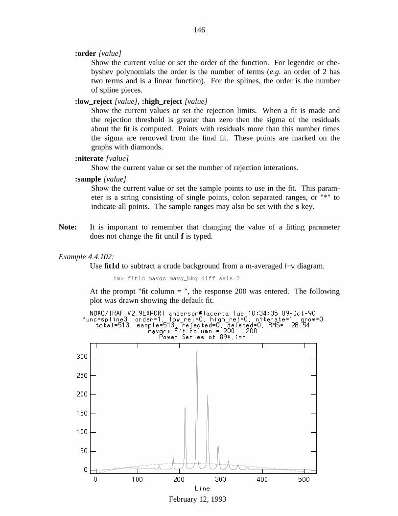
146

:order [value]Show the current value or set the order of the function. For legendre or che-byshev polynomials the order is the number of terms (e.g. an order of 2 hastwo terms and is a linear function). For the splines, the order is the numberof spline pieces.

:low_reject [value], :high_reject [value]Show the current values or set the rejection limits. When a fit is made andthe rejection threshold is greater than zero then the sigma of the residualsabout the fit is computed. Points with residuals more than this number timesthe sigma are removed from the final fit. These points are marked on thegraphs with diamonds.

:niterate [value]Show the current value or set the number of rejection interations.

:sample [value]Show the current value or set the sample points to use in the fit. This param-eter is a string consisting of single points, colon separated ranges, or "*" toindicate all points. The sample ranges may also be set with the s key.

Note: It is important to remember that changing the value of a fitting parameterdoes not change the fit until f is typed.

Example 4.4.102:Use fit1d to subtract a crude background from a m-averaged l−ν diagram.

im> fit1d mavgc mavg_bkg diff axis=2

At the prompt "fit column = ", the response 200 was entered. The followingplot was drawn showing the default fit..

February 12, 1993

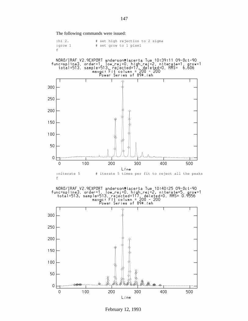
147

The following commands were issued:

:hi 2. # set high rejection to 2 sigma:grow 1 # set grow to 1 pixelf

.

:niterate 5 # iterate 5 times per fit to reject all the peaksf

.

February 12, 1993

148

s # mark the start of a section at about line 50again: s # mark the end the section at line 500f

.

q # quit fitting this columnmavg: Fit column = 100 # fit column 100

.

February 12, 1993

149

q # quit fitting this columnmavg: Fit column = 40 # check the fit on column 40

.

q # quit fitting this columnmavg: Fit column = <CR> # Exit interactive mode

At this point fit1d goes off and fits every column (in this case) using thecurrent fit parameters. The switching from column to column as demon-strated above is useful for checking that the fit will be globally applicable.

The original l−ν diagram is shown below on the left. The middle diagram isthe result from the fit1d example just shown. The figure at the right is alsothe result of fit1d, but with an order=7, cubic spline fitting function. Thebackground is not accurately subtracted in these examples; however, many ofthe fainter features are now more easily seen.

February 12, 1993

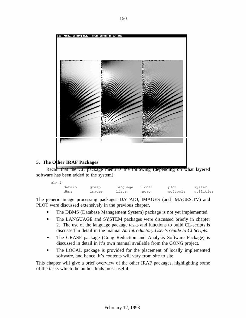
150

.

5. The Other IRAF Packages

Recall that the CL package menu is the following (depending on what layeredsoftware has been added to the system):

cl> ?dataio grasp language local plot systemdbms images lists noao softools utilities

The generic image processing packages DATAIO, IMAGES (and IMAGES.TV) andPLOT were discussed extensively in the previous chapter.

� The DBMS (Database Management System) package is not yet implemented.� The LANGUAGE and SYSTEM packages were discussed briefly in chapter

2. The use of the language package tasks and functions to build CL-scripts isdiscussed in detail in the manual An Introductory User’s Guide to Cl Scripts.

� The GRASP package (Gong Reduction and Analysis Software Package) isdiscussed in detail in it’s own manual available from the GONG project.

� The LOCAL package is provided for the placement of locally implementedsoftware, and hence, it’s contents will vary from site to site.

This chapter will give a brief overview of the other IRAF packages, highlighting someof the tasks which the author finds most useful.

February 12, 1993

151

5.1. The NOAO Package

The NOAO package is comprised of many subpackages each of which containstasks specific to the reduction and analysis of the various instruments available forKPNO night time use. However, many of the tasks in various packages can be used formore general applications, and the user is encouraged to at least gain a cursoryknowledge of the these tasks. The following is the help page for the NOAO package:

no> helprootnoao.noao:

artdata - Artificial data generation package [up]astrometry - Astrometry package

astutil - Astronomical utilities package [up]digiphot - Digital stellar photometry package [up]

focas - Faint object classification and analysis packageimred - Image reductions package [up]

mtlocal - Magtape i/o for special NOAO format tapes [up]onedspec - One dimensional spectral red & analysis package [up]

proto - Prototype (temporary, contributed) tasks [up]surfphot - Galaxy isophotal analysis packagetwodspec - Two dimensional spectral red & analysis package [up]

no>

5.1.1. PROTO

This package may prove to be the most useful to the general user. The tasks inthis package are prototype tasks. When the function and usage becomes more stable(and possibly more general and bug free) they are moved to the appropriate systempackage. The IMAGES tasks imstack and imslice are tasks that have migrated fromthe PROTO package.

noao.proto:binfil - Create a binary file from an IRAF image

binpairs - Bin pairs of (x,y) points in log separationbscale - Brightness scale images: new = (old - bzero) / bscaleepix - Edit pixels in an image

fields - Extract specified fields from a listimalign - Register and shift a list of images

imcentroid - Compute relative shifts for a list of imagesfixpix - Fix bad pixels by linear interpolation from nearby pixelsimcntr - Locate the center of a stellar imageimedit - Examine and edit pixels in images

imexamine - Examine images using image display, graphics, and textimfunction - Apply a function to the image pixel valuesimreplace - Replace pixels in a range by a constantimscale - Scale an image to a specified (windowed) meanimslice - Slice images into images of lower dimensionimstack - Stack images into an image of higher dimensionimtitle - Change the title of an imageinterp - Interpolate for a value in a table of X,Y pairsirafil - Create an IRAF image from a binary data file

iralign - Align the mosaiced image produced by irmosaicirmatch1d - Align and intensity match image produced by irmosaic (1D)irmatch2d - Align and intensity match image produced by irmosaic (2D)irmosaic - Mosaic an ordered list of images onto a grid

join - Join text files line by linemkhistogram - List or plot the histogram of a data stream

February 12, 1993

152

ndprep - Make neutral density filter calibration imageradplt - Plot a radial profile of a stellar imageslitpic - Generate IRAF image of aperture slit mask

toonedspec - Extract lines/columns from 2D spectra to 1D spectratvmark - Mark objects on the image display

fieldsThis is a list processing tool used to extract whitespace-separated fields from linesof the specified text files and print the extracted fields to STDOUT. The parame-ters are as follows:

pr> lpar fieldsfiles = Files from which to extract fields

fields = Fields to extract(lines = "1-9999") Lines from which to extract fields

(quit_if_miss = no) Quit on missing field?(print_file_n = no) Print file names if multiple files?

(mode = "ql")

The fields of a line are numbered from 1 up to a newline character; those fields tobe extracted are specified as a range of numbers given by the fields parameter.

If a specified field is missing from a selected line the action taken is determined bythe quit_if_missing flag.

Example 5.1.103:Extract columns 1 and 3 from file mydata.dat and pipe them to task graph.

pr> fields mydata.dat "1,3" | graph

Example 5.1.104:Extract columns 1, 3 and 5 through 10 from file mydata.dat and output themto a new file selected.dat.

pr> fields mydata.dat "1,3,5-10" > selected.dat

joinThis task reads lines from each of the input text files and joins them into one lineseparated by the specified delimiter. This is useful for making multicolumn filesfrom individual files. The parameters are as follows:

pr> lpar joinlist1 = List of input files to be joinedlist2 = List of input files to be joined

(output = "STDOUT") Output file(delim = " ") Delimiter between file lines

(missing = "Missing") Marker for missing lines(maxchars = 161) Maximum number of output characters per line(shortest = yes) Quit at end of shortest file?(verbose = yes) Print verbose warnings?

(mode = "ql")

The list of input files may be given in either list1 or with list2. The second list is

February 12, 1993

153

only used if two arguments are given on the command line. This feature is pro-vided for compatibility with an earlier version of this task which only joined twofiles given separately.

If the shortest parameter is set then the join operation is terminated with the lastline from the shortest file. If it is not set then the string from the parameter miss-ing is substituted for input from the shorter files until the end of the longest file isreached. Note that the delimiter will still be placed between input lines even whensuch lines are missing.

There is no limit to the possible number of characters per output line but theparameter maxchars may be used to truncate long lines. This can be importantbecause many IRAF tasks read files a line at a time with a fixed size line buffer.Also other tasks and host programs (for example UNIX/vi) have line limits aswell.

Example 5.1.105:Join a set of single column files into one multicolumn file called alldata.Separate the columns by tabs.

pr> join data* out=alldata delim=" "

interpThis task computes an interpolated value from a table of x,y pairs. The parametersare as follows:

pr> lpar interptbl_file = "" File containing table of x-y pairs

input = "STDIN" input for x-interpolant valuesx1 = First point in range of generated curvex2 = Last point in range of generated curvedx = Interval between generated points

(int_mode = "spline") Use linear or spline interpolator(curve_gen = no) Generate a curve between specified limits

(mode = "ql")

The pairs of X,Y values are read from the tbl_file. There must be at least 1 pair inthe file. The table is then used to interpolate or extrapolate new y-values for givenx-values.

The input x-values may come from a file including STDIN (if curve_gen=no), orthey may be internally generated (if curve_gen=yes) to produce a finely sampledversion of the table. This may be useful for plotting a smooth curve through aseries of points.

The table X,Y values must be in a monotonic order, either ascending or descend-ing. No restriction is made on spacing.

If only one point is present in the table, all returned interpolated values will havethe value at that point. If only two points are present, linear interpolation (or extra-polation) will be used. If additional points are present, an obscure but reliable

February 12, 1993

154

algorithm is used to interpolate (or extrapolate).

Example 5.1.106:Interactively spline interpolate at various points in the table shown below.

pr> ty mydata.dat0 01 12 43 94 165 96 47 18 0pr> interp mydata.datinput for x-interpolant values (STDIN):1.5

1.5 2.252.5

2.5 6.253.5

3.5 12.54.5

4.5 12.510.

10. -0.5CTRL-Zpr>

Example 5.1.107:Use the spline interpolator to generate a smooth curve at intervals of 0.1 inthe range -5 to 15. Overplot the data and the generated curve.

pr> interp mydata.dat curve+ int=spline x1=-5 x2=15 dx=.1 | graphpr> graph mydata.dat point+ app+

February 12, 1993

155

.

mkhistogramThis task is used to print or plot the histogram of a data stream. The parametersare as follows:

pr> lpar mkhistfile = File namenbins = 1 Number of bins in histogram

(z1 = INDEF) Minimum histogram intensity(z2 = INDEF) Maximum histogram intensity

(listout = yes) List instead of plot histogram(device = "stdgraph") output graphics device

(mode = "ql")

The input, file may be a text file, or input through STDIN (e.g., from a pipe).

If the z1 or z2 are undefined the data minimum or maximum is used.

If listout = yes, the histogram is listed on STDOUT. This is useful for saving theoutput for use by some other plot package (e.g., Mongo).

Example 5.1.108:Plot the histogram of mode fullwidths between the 0.5 and 1.5 with a binsizeof 0.05 to device "lw7".

pr> mkhist modewidths nbins=20 z1=0.5 z2=1.5

February 12, 1993

156

imfunctionThis task applies a function to an image. The parameters are as follows:

pr> lpar imfuncinput = Input images

output = Output imagesfunction = "log10" Function

(mode = "ql")

The current function options are the base ten logarithm and antilogarithm log10and alog10, the square root sqrt, and the absolute value abs.

tvmarkThis task marks objects on the display by writing directly into the specified framebuffer. tvmark can draw on any device supported by the IRAF display program.The parameters are as follows:

pr> lpar tvmarkframe = 1 Default frame number for displaycoords = "" Input coordinate list

(logfile = "") Output log file(autolog = no) Automatically log each marking command(outimage = "") Output snapped image(deletions = "") Output coordinate deletions list(commands = "") Image cursor: [x y wcs] key [cmd]

(mark = "point") The mark type(radii = "0") Radii in image pixels of concentric circles

(lengths = "0") Lengths and width in image pixels of concentric(font = "raster") Default font(color = 255) Gray level of marks to be drawn(label = no) Label the marked coordinates

(number = no) Number the marked coordinates(nxoffset = 0) X offset in display pixels of number(nyoffset = 0) Y offset in display pixels of number(pointsize = 3) Size of dot in display pixels

(txsize = 1) Size of text and numbers in font units(tolerance = 1.5) Tolerance for deleting coordinates in image pix

(interactive = no) Mode of use(mode = "ql")

After marking, the contents of the frame buffer may be written out to the IRAFimage outimage. The output image is equal in size and intensity to the contents ofthe frame buffer displayed at the time of writing.

In interactive mode objects to be marked may be selected interactively using theimage cursor or read from the text file coords. Objects in the coordinate list maybe selected individually by number, in groups by specifying a range of numbers,or the entire list may be read. New objects may be added to the list interactivelyusing the append keystroke command.

In batch mode cursor commands may be read from a text file specified by theparameter commands.

The mark commands entered in interactive mode can be saved in the text filelogfile. If autolog is enabled and logfile is defined all cursor commands are

February 12, 1993

157

automatically logged. If autolog is turned off then the user can select which com-mands are to be logged interactively using the interactive keep keystroke.

In interactive mode tvmark maintains a scratch buffer. The user opens the scratchbuffer by issuing a save command which saves the current contents of the framebuffer in a temporary IRAF image. The user can continue marking and ifunsatisfied with the results restore the last saved copy of the frame buffer with therestore command.

A snapshot of the frame buffer can be saved permanently by using the write com-mand. These snapped images can be redisplayed by setting the display taskparameter ztrans = "none".

The following keystroke commands are available:

? Print help+ Mark the cursor position with +x Mark the cursor position with xd Mark the cursor position with a dotc Draw defined concentric circles around the cursor positionr Draw defined concentric rectangles around the cursor positions Draw line segments, 2 keystrokesv Draw a circle, 2 keystrokesb Draw a rectangle, 2 keystrokesf Draw filled rectangle, 2 keystrokese Mark region to be erased and restored, 2 keystrokes- Move to previous object in the coordinate listm Move to next object in the coordinate listp Mark the previous object in the coordinate listn Mark next object in the coordinate listl Mark all the objects in the coordinate listo Rewind the coordinate lista Append object at cursor position to coordinate list and marku Delete object nearest the cursor position in the coordinate list and markk Keep last cursor commandq Exit tvmark

The following colon commands are available:

:show List the tvmark parameters:move N Move to Nth object in coordinate list:next N M Mark objects N to M in coordinate list:text [string] Write text at the cursor position:save Save the current contents of frame buffer:restore Restore last saved frame buffer:write [imagename] Write the contents of frame buffer to an image

The following parameters can be shown or set with colon commands:

:frame [number]:outimage [imagename]:coords [filename]

February 12, 1993

158

:logfile [filename]:autolog [yes/no]:mark [point|line|circle|rectangle|cross|plus]:radii [r1,...,rN]:lengths [l1,...,lN] [width]:font [raster]:color [number]:number [yes/no]:label [yes/no]:txsize [1,2,..]:pointsize [1,3,5...]

The current IMTOOL colors are as follows:

0 = sunview background color (normally white)1-200 = frame buffer data values, windowed

201 = cursor color (white) 202 = black203 = white 204 = red205 = green 206 = blue207 = yellow 208 = cyan209 = magenta 210 = coral211 = maroon 212 = orange213 = khaki 214 = orchid215 = turquoise 216 = violet217 = wheat

218-254 = reserved for use by other windows255 = black (sunview foreground color)

Example 5.1.109:The following command file was initially created with autolog=yes, andedited to produce the results shown in Example 4.2.1. Note that the cursorfile format is the same as for graphics cursor files, except that the WCSnumber is 101.

pr> type tv1.tvmark6.5 188.5 101 : color 2026.5 188.5 101 : frame 16.5 188.5 101 : txsize 290. 740. 101 : text Contrast = 0.1620. 740. 101 : text Contrast = 0.251160. 740. 101 : text Contrast = 0.590. -50. 101 : text Contrast = 0.75620. -50. 101 : text Contrast = 1.01160. -50. 101 : text Contrast = 1.2pr> set stdimage = imt800pr> disp dev$pix 1 xc=.16 yc=.74 cont=.1 xm=.50 ym=.50pr> disp dev$pix 1 xc=.5 yc=.74 cont=.25 xm=.50 ym=.50 er-pr> disp dev$pix 1 xc=.84 yc=.74 cont=.5 xm=.50 ym=.50 er-pr> disp dev$pix 1 xc=.5 yc=.25 cont=1. xm=.50 ym=.50 er-pr> disp dev$pix 1 xc=.84 yc=.25 cont=1.2 xm=.50 ym=.50 er-pr> disp dev$pix 1 xc=.16 yc=.25 cont=.75 xm=.50 ym=.50 er-pr> tvmark 1 "" command=tv1.tvmark

February 12, 1993

159

Example 5.1.110:Label the ridges on an l−ν diagram.

pr> reset stdimage = imt800pr> disp mavgc 4 xc=.35 yc=.54 xm=1.5 ym=1.4 order=1 zs- zr- z1=450. z2=-5.pr> tvmark 1 "" int+ log=mavgc.tvmark auto+:color 202 [change color to black]:txsize 2 [set text size][position cursor for "Nu" label]

:text Nu[position cursor for "L" label]:text L[position cursor for text]

:text L-Nu Diagram[position cursor for text]

:text (June 8, 1989)[position cursor for text]

:text M = M-averaged[position cursor for text]

:text T = 12.75 hrs:txsize 1 [set text size][position cursor for text]

:text 250[position cursor for text]

:text 0[position cursor for text]

:text 0[position cursor for text]

:text 6679[position cursor for text]

:text (microHz):txsize 2 [set text size][position cursor to draw line]s[position cursor at other end of line to be drawn]s:text n=1[position cursor for text]

:text n=3[position cursor for text]

:text n=5[position cursor for text]

:text n=7[position cursor for text]

:text n=9[position cursor to draw line]s[position cursor at other end of line to be drawn]s:text n=11[position cursor to draw line]s[position cursor at other end of line to be drawn]s:text n=13[position cursor to draw line]s[position cursor at other end of line to be drawn]s

February 12, 1993

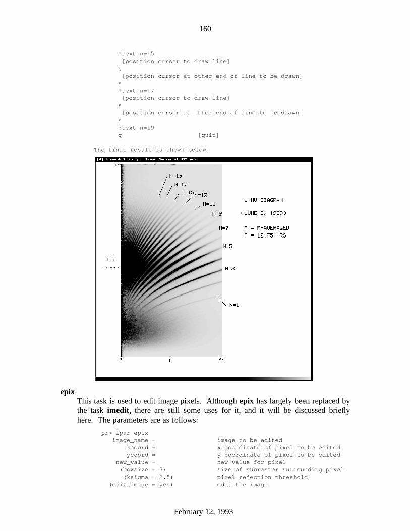
160

:text n=15[position cursor to draw line]s[position cursor at other end of line to be drawn]s:text n=17[position cursor to draw line]s[position cursor at other end of line to be drawn]s:text n=19q [quit]

The final result is shown below..

epixThis task is used to edit image pixels. Although epix has largely been replaced bythe task imedit, there are still some uses for it, and it will be discussed brieflyhere. The parameters are as follows:

pr> lpar epiximage_name = image to be edited

xcoord = x coordinate of pixel to be editedycoord = y coordinate of pixel to be edited

new_value = new value for pixel(boxsize = 3) size of subraster surrounding pixel(ksigma = 2.5) pixel rejection threshold

(edit_image = yes) edit the image

February 12, 1993

161

(verbose = yes) print subraster and median value(mode = "ql")

A subraster boxsize pixels square is extracted centered on the pixelimage_name[xcoord,ycoord].

If verbose=yes, the values of the pixels in the subraster are printed on the standardoutput along with the rejection mean and median of the subraster.

If edit_image=yes the program will ask for the new_value and edit the image. Ifnew_value was not given on the command line, then the user has the opportunityto look at the verbose output before choosing the replacement value.

The ksigma parameter sets the rejection threshold for the iterative rejection algo-rithm used to compute the mean.

Example 5.1.111:Replace specified pixels in the image raw1 with 0.

pr> epix raw1 5 10 0. ver-pr> epix raw1 250 10 0. ver-pr> epix raw1 256 252 0. ver-

Example 5.1.112:Replace a bad pixel at (100,55) of image myimage, with the median of a 5pixel box surrounding it.

pr> epix myimage 100 55 box=598 99 100 101 102

53 2400449. 2399708. 2402400. 2403735. 2404888.54 2398644. 2404149. 2404547. 2401151. 2399032.55 2401287. 2404118. 1.2345E9 2404756. 2403233.56 2405423. 2400972. 2400747. 2408607. 2406847.57 2401085. 2399510. 2400980. 2404984. 2408453.

median 2403233., mean 2402905., sigma 2785.462, sample 24 pixelsnew value for pixel: 2403233.

fixpixThis task fixes bad pixels by linear interpolation from nearby pixels. The parame-ters are as follows:

pr> lpar fixpiximages = Images to be modified

badpixels = "" Bad pixel regions file(verbose = no) Print the image name and bad regions?

(mode = "ql")

badpixels is a file containing the regions of bad pixels. A region is described byfour whitespace separated numbers consisting of the first and last columns of thebad region and the first and last lines of the bad region. The file may be STDIN toread from the standard input.

February 12, 1993

162

The type of interpolation is determined as follows:

(1) If the bad region spans entire lines then the interpolation is from neighboringlines.

(2) If the bad region spans entire columns then the interpolation is from neigh-boring columns.

(3) If the bad region contains more lines than columns then the interpolation isfrom neighboring columns.

(4) If the bad region contains the same or more columns than lines then the inter-polation is from neighboring lines.

That is, the interpolation is done across the shortest dimension of the bad pixelregion.

If the bad region borders the edge of the image then the interpolation is by replica-tion of the first good pixel in the direction of interpolation and otherwise linearinterpolation between the bordering lines or columns is used.

Example 5.1.113:Clean out the bad pixel regions from a 2048×2048 square image.

pr> type badpix298 299 257 318 [bad region]684 684 322 2044 [partial bad column]700 700 1 2044 [bad column]1340 1342 1604 2044 [partial bad columns]1325 1327 1610 2044 [partial bad columns]1470 1470 1 2044 [bad column]pr> fixpix data*.imh badpix

imexamineThis task allows one to examine images using image display, plots, and text simul-taneously. Commands are given using the image display cursor and/or graphicscursor. This task brings together many of the features of the IRAF image displayand graphics facilities with some simple image analysis capabilities. The parame-ters are as follows:

pr> lpar imexaminput = images to be examinedframe = 1 display frameimage = image name

(logfile = "") logfile(keeplog = no) log output results(defkey = "a") default key for cursor list input

(autoredraw = yes) automatically redraw graph(allframes = yes) use all frames for displaying new images

(nframes = 0) number of display frames (0 to autosense)(ncstat = 5) number of columns for statistics(nlstat = 5) number of lines for statistics

(graphcur = "") graphics cursor input(imagecur = "") image display cursor input(graphics = "stdgraph") graphics device(display = "display(image=’$1’,frame=$2)") display command template

February 12, 1993

163

(use_display = yes) enable direct display interaction(mode = "ql")

The various graphs and the aperture sum command have parameters defined inadditional parameter sets. The parameter sets are hidden tasks with the first char-acter being the cursor command graph key that uses the parameters followed by"imexam". The parameter sets are

cimexam Parameters for column plotseimexam Parameters for contour plotshimexam Parameters for histogram plotslimexam Parameters for line plotsrimexam Parameters for radial profile plots and aperture sumssimexam Parameters for surface plotsvimexam Parameters for vector plots (centered and endpoint)

The various parameters for these subsets are the same as those for other taskswhich perform the same function (e.g., surface plots). See the imexamine helppage for details.

If use_display is yes the image display is used to examine images. When no inputlist is specified images may be loaded with the d key, frames selected with n, p,and :select, and the scaled contents of the display frame buffer examined if theimage itself is not available.

The d command displays an image using the template CL command given byparameter display. Usually this is the standard IRAF tv.display command thoughin some circumstances other commands like plot.contour may be used. Thiscommand may be used to display an image even if use_display=no.

Generally the image cursor is used to select points in the images to be examinedand the key typed selects a particular operation. In addition to the image cursorthe graphics cursor is sometimes useful. First, it gives access to the graphics cur-sor mode commands such as annotating, saving or printing a graph, expanding androaming, and printing cursor positions. Second, it can give a better perspective onthe data for cursor positions than the image cursor. And lastly, it may be neededwhen an image display is not available. The commands g and i select between thegraphics and image cursors. Initially the image cursor is read.

There are some special features associated with cursor input in IRAF which mightbe useful in some circumstances. Read the help pages for this task for moredetails.

The following are the cursor commands:

? Print helpa Aperture sum, moment parameters, and gaussian fit

col line mag flux sky npixels rmom ellip pa peak fwhmb Box coordinates for two cursor positions - c1 c2 l1 l2

February 12, 1993

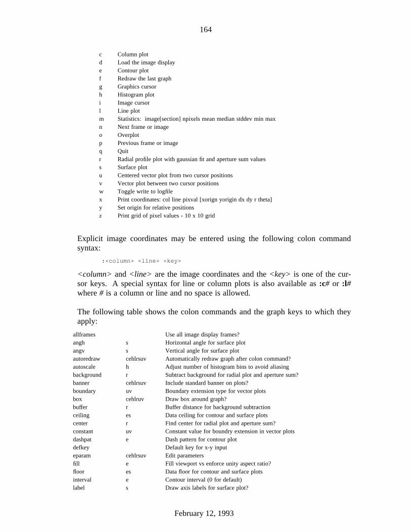
164

c Column plotd Load the image displaye Contour plotf Redraw the last graphg Graphics cursorh Histogram ploti Image cursorl Line plotm Statistics: image[section] npixels mean median stddev min maxn Next frame or imageo Overplotp Previous frame or imageq Quitr Radial profile plot with gaussian fit and aperture sum valuess Surface plotu Centered vector plot from two cursor positionsv Vector plot between two cursor positionsw Toggle write to logfilex Print coordinates: col line pixval [xorign yorigin dx dy r theta]y Set origin for relative positionsz Print grid of pixel values - 10 x 10 grid

Explicit image coordinates may be entered using the following colon commandsyntax:

:<column> <line> <key>

<column> and <line> are the image coordinates and the <key> is one of the cur-sor keys. A special syntax for line or column plots is also available as :c# or :l#where # is a column or line and no space is allowed.

The following table shows the colon commands and the graph keys to which theyapply:

allframes Use all image display frames?angh s Horizontal angle for surface plotangv s Vertical angle for surface plotautoredraw cehlrsuv Automatically redraw graph after colon command?autoscale h Adjust number of histogram bins to avoid aliasingbackground r Subtract background for radial plot and aperture sum?banner cehlrsuv Include standard banner on plots?boundary uv Boundary extension type for vector plotsbox cehlruv Draw box around graph?buffer r Buffer distance for background subtractionceiling es Data ceiling for contour and surface plotscenter r Find center for radial plot and aperture sum?constant uv Constant value for boundry extension in vector plotsdashpat e Dash pattern for contour plotdefkey Default key for x-y inputeparam cehlrsuv Edit parametersfill e Fill viewport vs enforce unity aspect ratio?floor es Data floor for contour and surface plotsinterval e Contour interval (0 for default)label s Draw axis labels for surface plot?

February 12, 1993

165

logfile Log file namelogx chlruv Plot x axis logrithmically?logy chlruv Plot y axis logrithmically?magzero r Magnitude zero for aperture summajrx cehlruv Number of major tick marks on x axismajry cehlruv Number of major tick marks on y axismarker chlruv Marker type for graphminrx cehlruv Number of minor tick marks on x axisminry cehlruv Number of minor tick marks on y axisnaverage cluv Number of columns, lines, vectors to averagenbins h Number of histogram binsncolumns ehs Number of columns in contour, histogram, or surface plotncontours e Number of contours (0 for default)ncstat Number of columns in statistics boxnhi e hi/low marking option for contoursnlines ehs Number of lines in contour, histogram, or surface plotnlstat Number of lines in statistics boxpointmode chluv Plot points instead of lines?radius r Radius of object aperture for radial plot and photmetryround cehlruv Round axes to nice values?rplot r Radius to plot in radial profile plotselect Select image or display frameszmarker chlruv Size of marks for point modeticklabels cehlruv Label ticks?title cehlrsuv Optional title for graphtop_closed h Close last bin of histogramunlearn cehlrsuv Unlearn parameters to default valueswidth r Width of background annulus for aperture sumx [min max] chlruv Range of x to be plotted (no values for autoscaling)xlabel cehlrsuv Optional label for x axisxorder r X order of surface for background subtractiony [min max] chlruv Range of y to be plotted (no values for autoscaling)ylabel cehlrsuv Optional label for y axisyorder r Y order of surface for background subtractionz1 h Lower intensity value limit of histogramz2 h Upper intensity value limit of histogramzero e Zero level for contour plot

Example 5.1.114:Examine rawiii. Contour and vector plot the central sunspot group.

pr> imexam rawiii 1

used mouse to magnify image and center sunspot group in the display window.

February 12, 1993

166

.

e [contour plot, cursor was set at center of large spot]

The following is a screen dump. The resolution is too poor to see the display window contents..

February 12, 1993

167

g [switch to graphics cursor]:epar eimexam [edit contour pset: ncolumns=51, nline=51, and ncontour=10]CTRL-Z [exit epar, plot updates automatically].

:.snap lw7 [make a hardcopy of contour plot]:epar vimexam [edit vector pset: set naverage=5; CRTL-Z to exit]v [mark centers of upper & lower spots for vector plot].

:.snap lw7 [make a hardcopy of vector plot]q [quit]

February 12, 1993

168

imeditThis task allows the user to examine and edit regions of images. This may bedone interactively using an image display and cursor or noninteractively using alist of positions and commands. The parameters are:

pr> lpar imeditinput = Images to be editedoutput = Output images

(cursor = "") Cursor input(logfile = "") Logfile for record of cursor commands(display = yes) Display images?

(autodisplay = yes) Automatic image display?(autosurface = no) Automatic surface plots?

(aperture = "circular") Aperture type(radius = 2.) Substitution radius(search = 2.) Search radius(buffer = 1.) Background buffer width(width = 2.) Background width(xorder = 2) Background x order(yorder = 2) Background y order(value = 0.) Constant value substitution(sigma = INDEF) Added noise sigma(angh = -33.) Horizontal viewing angle (degrees)(angv = 25.) Vertical viewing angle (degrees)

(command = "display $image 1 erase=$erase fill=yes order=0 >& dev$null") D(graphics = "stdgraph") Graphics device(default = "b") Default option for x-y input(fixpix = no) Fixpix style input?(mode = "ql")

A list of input images and a matching list of output images are specified. The out-put images are only created if the input image is modified (except by an explicit"write" command). If no output list is specified (an empty list given by "") thenthe modified images are written back to the input images.

The images are edited in a temporary buffer image called "epixbuf" and so anyediting mistakes will not be disasterous unless the user specifically overwrites theinput image.

Like imexamine, imedit has many features. The user is encouraged to carefullyread the help pages. The following is only a brief command summary.

Regions of the image to be examined or edited are selected by one or two cursorcommands. The single cursor commands define the center of an aperture. Theshape of the aperture, circular or square, is specified by the aperture parameter andthe radius (or half the edge of a square) is specified by the radius parameter. Theradius may be zero to select a single pixel.

Once a region has been defined a background region may be required to estimatethe background for replacement. The background region is an annulus of the sameshape separated by a buffer width, given by the parameter buffer, and having awidth given by the parameter width.

February 12, 1993

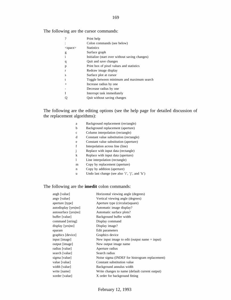
169

The following are the cursor commands:

? Print help: Colon commands (see below)<space> Statisticsg Surface graphi Initialize (start over without saving changes)q Quit and save changesp Print box of pixel values and statisticsr Redraw image displays Surface plot at cursort Toggle between minimum and maximum search+ Increase radius by one- Decrease radius by oneI Interrupt task immediatelyQ Quit without saving changes

The following are the editing options (see the help page for detailed discussion ofthe replacement algorithms):

a Background replacement (rectangle)b Background replacement (aperture)c Column interpolation (rectangle)d Constant value substitution (rectangle)e Constant value substitution (aperture)f Interpolation across line (line)j Replace with input data (rectangle)k Replace with input data (aperture)l Line interpolation (rectangle)m Copy by replacement (aperture)n Copy by addition (aperture)u Undo last change (see also ’i’, ’j’, and ’k’)

The following are the imedit colon commands:

angh [value] Horizontal viewing angle (degrees)angv [value] Vertical viewing angle (degrees)aperture [type] Aperture type (circular|square)autodisplay [yes|no] Automatic image display?autosurface [yes|no] Automatic surface plots?buffer [value] Background buffer widthcommand [string] Display commanddisplay [yes|no] Display image?eparam Edit parametersgraphics [device] Graphics deviceinput [image] New input image to edit (output name = input)output [image] New output image nameradius [value] Aperture radiussearch [value] Search radiussigma [value] Noise sigma (INDEF for histrogram replacement)value [value] Constant substitution valuewidth [value] Background annulus widthwrite [name] Write changes to name (default current output)xorder [value] X order for background fitting

February 12, 1993

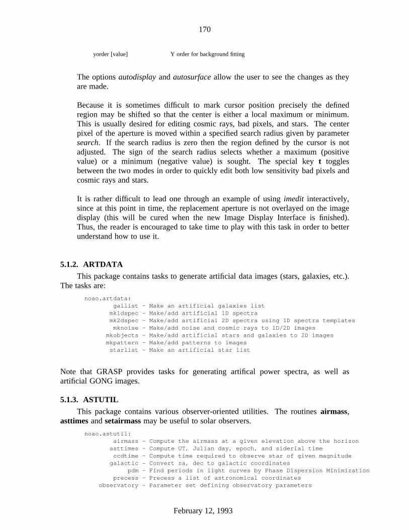
170

yorder [value] Y order for background fitting

The options autodisplay and autosurface allow the user to see the changes as theyare made.

Because it is sometimes difficult to mark cursor position precisely the definedregion may be shifted so that the center is either a local maximum or minimum.This is usually desired for editing cosmic rays, bad pixels, and stars. The centerpixel of the aperture is moved within a specified search radius given by parametersearch. If the search radius is zero then the region defined by the cursor is notadjusted. The sign of the search radius selects whether a maximum (positivevalue) or a minimum (negative value) is sought. The special key t togglesbetween the two modes in order to quickly edit both low sensitivity bad pixels andcosmic rays and stars.

It is rather difficult to lead one through an example of using imedit interactively,since at this point in time, the replacement aperture is not overlayed on the imagedisplay (this will be cured when the new Image Display Interface is finished).Thus, the reader is encouraged to take time to play with this task in order to betterunderstand how to use it.

5.1.2. ARTDATA

This package contains tasks to generate artificial data images (stars, galaxies, etc.).The tasks are:

noao.artdata:gallist - Make an artificial galaxies list

mk1dspec - Make/add artificial 1D spectramk2dspec - Make/add artificial 2D spectra using 1D spectra templatesmknoise - Make/add noise and cosmic rays to 1D/2D images

mkobjects - Make/add artificial stars and galaxies to 2D imagesmkpattern - Make/add patterns to imagesstarlist - Make an artificial star list

Note that GRASP provides tasks for generating artifical power spectra, as well asartificial GONG images.

5.1.3. ASTUTIL

This package contains various observer-oriented utilities. The routines airmass,asttimes and setairmass may be useful to solar observers.

noao.astutil:airmass - Compute the airmass at a given elevation above the horizonasttimes - Compute UT, Julian day, epoch, and siderial timeccdtime - Compute time required to observe star of given magnitudegalactic - Convert ra, dec to galactic coordinates

pdm - Find periods in light curves by Phase Dispersion Minimizationprecess - Precess a list of astronomical coordinates

observatory - Parameter set defining observatory parameters

February 12, 1993

171

rvcorrect - Compute radial velocity correctionssetairmass - Compute effective airmass and middle UT for an exposure

5.1.4. DIGIPHOT

The digital photometry package currently consists of APPHOT, the Aperture Pho-temetry Package which incorporates DAOPHOT, the crowded field photometry softwareof Peter Stetson, at DAO. A manual entitled A User’s Guide to the IRAF Apphot Pack-age, is available. Also, A User’s Guide to Stellar CCD Photometry with IRAF is avail-able, which discusses DAOPHOT/IRAF in particular.

5.1.5. IMRED

This package contains tasks for the reduction and analysis of digital data from thevarious KPNO night time instruments, the Solar Vacuum telescope and the PDS Micro-densitometer.

noao.imred:bias - General bias subtraction tools

ccdred - CCD reductionscoude - Coude reductionsdtoi - Density to Intensity reductions for photographic plates

echelle - Echelle spectra reductionsgeneric - Generic image reductions tools

iids - KPNO IIDS spectral reductionsirred - KPNO IR camera reductions

irs - KPNO IRS spectral reductionsmsred - Reduction package for multiple spectra data

observatory - Print observatory parameterssetairmass - Set midtime airmass and universal time

specphot - Spectrophotometric reductionsvtel - Solar vacuum telescope image reductions

Routines of general use for CCD reductions (i.e., overscan, bias, dark and flat fieldcorrections) can be found in the subpackages BIAS and GENERIC. Pipeline CCDreductions are performed from the package CCDRED.

imred.bias:colbias - Fit and subtract an average column biaslinebias - Fit and subtract an average line bias

imred.generic:background - Fit and subtract a line or column backgroundcosmicrays - Detect and replace cosmic rays

darksub - Scale and subtract a dark count imageflat1d - Make flat field by fitting a 1D func. to the lines or columnsflatten - Flatten images using a flat field

normalize - Normalize imagesnormflat - Create a flat field by normalizing and replacing low values

imred.ccdred:badpiximage - Create a bad pixel mask image from a bad pixel fileccdgroups - Group CCD images into image listsccdhedit - CCD image header editorccdlist - List CCD processing informationccdproc - Process CCD imagesccdtest - CCD test and demonstration package

February 12, 1993

172

combine - Combine CCD imagescosmicrays - Detect and replace cosmic raysdarkcombine - Combine and process dark count imagesflatcombine - Combine and process flat field imagesmkfringecor - Make fringe correction images from sky imagesmkillumcor - Make flat field illumination correction images

mkillumflat - Make illumination corrected flat fieldsmkskycor - Make sky illumination correction images

mkskyflat - Make sky corrected flat field imagessetinstrument - Set instrument parameters

zerocombine - Combine and process zero level images

ADDITIONAL HELP TOPICSccdgeometry - Discussion of CCD coordinate/geometry keywords

ccdred - CCD image reduction packageccdtypes - Description of the CCD image types

flatfields - Discussion of CCD flat field calibrationsguide - Introductory guide to using the CCDRED package

instruments - Instrument specific data filessubsets - Description of CCD subsets

Two manuals discussing the IMRED package are available:

User’s Guide to the CCDRED PackageA User’s Guide to CCD Reductions with IRAF

5.1.6. MTLOCAL

This package contains site specific magnetic tape readers (and perhaps writers).At NOAO, this package has the routine for reading the old KPNO Camera Format andCyber tapes.

noao.mtlocal:ldumpf - List the permanent files on a Cyber DUMPF taper2df - Convert a CTIO 2-d frutti image into an IRAF image

rcamera - Convert a CAMERA image into an IRAF imagerdumpf - Convert IPPS rasters from a DUMPF tape to IRAF images

ridsfile - Convert IDSFILES from a DUMPF tape to IRAF imagesridsmtn - Convert mountain format IDS/IRS data to IRAF imagesridsout - Convert a text file in IDSOUT format to IRAF images

rpds - Convert a PDS image into an IRAF imagerrcopy - Convert IPPS rasters from an RCOPY tape to IRAF images

widstape - Convert ONEDSPEC spectra to IDSOUT text format

5.1.7. ONEDSPEC

This package contains tasks used for one-dimensional spectroscopic reduction andanalysis.

noao.onedspec:addsets - Add subsets of strings of spectrabatchred - Batch reductions of beam-switched data

bplot - Batch plots of spectrabswitch - Beam-switch strings of spectra to make obj-sky pairs

calibrate - Apply extinction and flux calibrations to spectracoincor - Correct spectra for detector count ratescombine - Combine spectra having different wavelength ranges

February 12, 1993

173

continuum - Fit the continuum in spectradispcor - Dispersion correct spectraflatdiv - Divide spectra by flat fieldflatfit - Sum and normalize flat field spectra

identify - Identify features in spectrum for dispersion solutionlcalib - List calibration file datamkspec - Generate an artificial spectrumnames - Generate a list of image names from a string

observatory - Print and define observatory parametersonedspec - Additional information about the ONEDSPEC packagepowercor - Apply a power-law flux correction correctionprocess - A task generated by BATCHRED

rebin - Rebin spectra to new dispersion parametersrefspectra - Assign wavelength reference spectra to other spectrareidentify - Automatically identify features in spectra

sensfunc - Create sensitivity functionsetdisp - Set dispersion image header parameters

sextract - Extract subspectra from dispersion corrected spectrasflip - Flip direction of dispersionshedit - Edit spectrum header parameters

sinterp - Interpolate a table of x,y pairs to create a spectrumslist - List spectrum header parameters

specplot - Stack and plot multiple spectrasplot - Preliminary spectral plot/analysis

standard - Identify standard stars to be used in sensitivity calcsubsets - Substract pairs in strings of spectra

sums - Generate sums of object and sky spectra by aperture

This package is described in the manual IIDS/IRS Data Reductions on IRAF with theOnedspec Package.

splotThe task splot is of general use in spectroscopic analysis by providing an interac-tive facility to display and analyze one- or two-dimensional spectra.

Like fit1d, all functions are driven by single keystroke commands when the graph-ics cursor is displayed or from cursor commands in a file. Some of the featuresavailable are line deblending, a variety of equivalent width algorithms, the applica-tion of arithmetic functions to the spectra, smoothing, wavelength scaling (or res-caling), etc.

Modified spectra may be saved as new images, or may overwrite existing images.

Anyone interested in spectroscopic analysis should read the help pages for thistask.

identify and reidentifyThese tasks are used to identify features in calibration spectra and computewavelength solutions to be used in the calibration of object spectra.

February 12, 1993

174

5.1.8. TWODSPEC

This package is the two dimensional analog of ONEDSPEC. Tasks are providedfor longslit and multi-slit reduction and analysis.

noao.twodspec:apextract - Aperture Extraction Packagelongslit - Longslit Packagemultispec - Multi-Spectra Extraction Package

observatory - Observatory parameterssetairmass - Set midtime airmass and universal time

setdisp - Set dispersion image header parameters

The are a number of user manuals describing various types of two dimensionalspectral reduction and analysis.

Reduction of Longslit Spectroscopic Data Using IRAF.Reduction of Echelle/CCD Data Using IRAF.IRAF Reduction of Coude/CCD Spectra.A User’s Guide to Multislit Spectroscopic Reductions with IRAF.Radial Velocity Measurements with IDENTIFY.

The Solar spectroscopist may find the LONGSLIT subpackage of interest. In par-ticular, the tasks identify and reidentify which are used in combination to track spec-tral features for the purposes of wavelength calibration, distortion correction and/orradial velocity mapping.

twodspec.longslit:background - Fit and subtract a line or column backgroundextinction - Apply atmospheric extinction corrections to imagesfitcoords - Fit user coordinates to image coordinatesfluxcalib - Apply flux calibration to imagesidentify - Identify features

illumination - Determine illumination calibrationreidentify - Reidentify features

response - Determine response calibrationtransform - Transform longslit images to user coordinates

5.2. The LISTS Package

This package contains tasks for basic list (i.e., text file) manipulation. Some ofthese tasks are useful for small processing jobs, but for large jobs, the user should con-sider TABLES (the external STSDAS package). The tasks of the LISTS package are asfollows:

lists.:average - Compute the mean and standard deviation of a listcolumns - Convert multicolumn file to separate fileslintran - Perform linear transformation of a list

rgcursor - Read the graphics cursor (makes a list)rimcursor - Read the image display cursor (makes a list)

table - Format a list of words into a tabletokens - Break a file up into a stream of tokensunique - Delete redundant elements from a listwords - Break a file up into a stream of words

February 12, 1993

175

Of these tasks, the author has found average, columns and lintran to be the most gen-erally useful.

averageThis task computes the average and standard deviation of a list of numbers. Theparameters are:

li> lpar averageoption = "new_sample" Type of sample (new_sample, add, subtract)

(opstring = )(addsub_flag = )(data_value = )

(n = )(sum = )

(sumsqrs = )(mean = )

(variance = )(sigma = )(mode = "ql")

Numeric input is read from STDIN with one number per line. Thus, input from afile must be done via a pipe (e.g., type filename | average) or input redirection(e.g., average < filename).

The mean, sigma and number of samples are written to the standard output andalso to the respective parameters so that they might be retrieved by other tasksand/or scripts (using imgets).

The parameter option allows the user to add or subtract new points from thecurrent list.

columnsThis task is the complement to the NOAO.PROTO task join. columns is used toreformat a multicolumn list file into separate files, such that one output file iscreated for each column in the input file. The parameters are as follows:

li> lpar columnfilename = Name of the input table filenumcols = Number of columns

(outroot = "col.") Root name of the output column files(mode = "ql")

The input file may have comments lines beginning with the character # which willbe ignored by the task.

Example 5.2.115:Break up a three-column mode frequency data file, mfdata, into three files ofrootname mfdata.

li> column mfdata 3 out=mfdata

February 12, 1993

176

lintranThis task performs a specified linear transformation (i.e., translation, scale androtation) on coordinate pairs. The parameters are as follows:

li> lpar lintranfiles =

(xfield = 1) field containing x coordinate(yfield = 2) field containing y coordinate

(min_sigdigit = 3) minimum significant digits to be output(x1 = 0.) current x origin(y1 = 0.) current y origin

(xscale = 1.) scale factor relative to current origin(yscale = 1.) scale factor relative to current origin(angle = 0.) rotation angle

(x2 = 0.) new x origin(y2 = 0.) new y origin

(radians = no) angle in radians?(mode = "ql")

Two fields of each input line are designated as the x and y coordinates to betransformed (default: fields 1, 2). All other fields are preserved across thetransformation. Comment lines (lines beginning with the character #) and blanklines are passed to the output unmodified.

Example 5.2.116:Shift a list of theoretical mode frequencies (l−ν) to match the scale of theJune 8, 1989 l−ν diagram so that they may be overlayed with the diagram onthe image display. For the l−ν diagram, mavgc, the frequency resolution is13.02083 µHz, and remember that the origin for images is (1,1).

li> imhead mavgcmavgc[251,512][real]: Power Series of 89*.imhli> disp mavg 1 xm=2.03984 or=1 # Fill imt512 windowli> head lnu.dat# mode frequencies# l nu (microHz)115 1941.14116 1947.18117 1953.57118 1959.52119 1965.95120 1971.69

li> lintran lnu.dat yscale=(1./13.02083) x2=1 y2=1 > lnu.tranli> head lnu.tran# 1987 mode frequencies# l nu (microHz)115. 150.08116. 150.543117. 151.034118. 151.491119. 151.985120. 152.426

li> graph lnu.tran box- po+ mark=plus wx1=1 wx2=251 wy1=1 wy2=512 >G lnu.pltli> imdkern lnu.plt color=203

A magnified portion of the overlayed l−ν diagram is shown below.

February 12, 1993

177

.

5.3. The UTILITIES Package

All of the tasks in this package are very useful, and straight forward to use. Whentransferring files between machines and via E-mail, the text filters are invaluable. Theavailable tasks are as follows:

utilities.:curfit - Fit data with Chebyshev, Legendre or spline curvedetab - Replace tabs with tabs and blanksentab - Replace blanks with tabs and blankslcase - Convert a file to lower case

polyfit - Fit polynomial to list of X,Y datasplit - Split a large file into smaller segments

translit - Replace or delete specified characters in a fileucase - Convert a file to upper caseurand - Uniform random number generator

curfitThis task is used to fit a curve (Chebyshev, Legendre or spline) to a list ofnumbers or an image section. The parameters are as follows:

ut> lpar curfitinput = "" input list of files or images

(function = "legendre") type of function to fit(weighting = "uniform") Weighting (uniform,user,statistical,instrumenta

(order = 4) order of the fit(interactive = yes) interactively tweak fit parameters?

February 12, 1993

178

(axis = 1) projection axis if input is an image(listdata = no) two column output list?(verbose = no) lengthy output format?(calctype = "double") Calculation datatype

(power = no) convert coeffecients to power series?(device = "stdgraph") name of interactive plotting device(cursor = "") Graphics cursor input(mode = "ql")

If data is read from an image, the axis parameter is used to reduce the dimen-sionality of the image; it specifies the axis along which the image is projected.For example, when axis=1, the image is compressed to a column; axis=2 wouldproject the image along a line; axis=3 indicates projection in the z direction, etc.

If the input is from a list, the data are sorted prior to fitting (input data must beordered in x).

When interactive=yes the user may adjust all the parameters of the fit, just aswhen using fit1d or any other interactive fitting task.

The final fit parameters are written to STDOUT with the format controlled byparameters verbose and listdata. By default, the function type, order, and resultingchi-square are printed as well as the coefficients and their standard deviations. Ifverbose is set to yes, a list of X, Y_calculated, Y_input, and W_input is alsoprinted.

If listdata is set to yes, the only printed output will be a listing of X, Yc, Y andW. This provides a list suitable as input to graph or any other list oriented utility.Setting listdata to yes overrides the verbose option.

When power = yes, the coefficients are converted to power series coefficients ofthe form

a 0 + a 1x + a 2x 2 + a 3x 3 . . .

Only Legendre and Chebyshev coefficients are converted; a conversion of splinecoefficients is meaningless.

polyfitThis task is used to calculate a polynomial weighted fit of specified order to theX,Y, SIGMAY data triples read from the input file, files, or STDIN. The parame-ters are:

ut> lpar polyfitinput = "STDIN" input filesorder = order of polynomial

(weighting = "uniform") Type of weighting (instrumental|uniform|statist(verbose = no) list calculated fit to data(listdata = no) list X-Y pairs only

(mode = "ql")

The resulting coefficients of the polynomial are printed on the first line of the

February 12, 1993

179

standard ouput. The uncertainty in each coefficient is printed on the next line inthe following format:

a 0 a 1 a 2 a 2 ...s 0 s 1 s 2 s 2 ...

where the polynomial has the form,

a 0 + a 1x + a 2x 2 + a 3x 3 . . .

If verbose=yes, the following additional information is listed: the resulting reducedchi-square, f-test, correlation coefficient, standard deviation of residuals, andnumber of items in the list.

The routine REGRES from the library of routines written by Bevington is used forthe fit; see Data Reduction and Error Analysis, by Bevington.

5.4. The SOFTOOLS Package

Most of the tasks in this package are used by those who are programming in SPP(the Subset Preprocessor Language). rtar and wtar are IRAF renditions of the UNIXtar utility, and operate in the same manner.

softools.:generic - Preprocess a generic source file

hdbexamine - Examine a help databaselroff - Lroff (line-roff) text formatter

mkhelpdb - Make (compile) a help databasemkmanpage - Make a manual page

mkpkg - Make or update an object library or packagemktags - Tag all procedure declarations in a set of files

mkttydata - Build cache for termcap/graphcap device entriesrmbin - Find/delete binary files in subdirectories

rmfiles - Find/delete files in subdirectoriesrtar - Read a TAR format archive filewtar - Write a TAR format archive filexc - Compile and/or link a program

xyacc - Build an SPP language parser

February 12, 1993