THE HEALTH EFFECTS

OF TWO INFLUENTIAL EARLY CHILDHOOD INTERVENTIONS

Gabriella Conti,

James Heckman,

and Rodrigo Pinto1

This Draft: September 30, 2014

1James Heckman is the Henry Schultz Distinguished Service Professor of Economics at the Universityof Chicago; Director, Center for the Economics of Human Development, University of Chicago; a ResearchFellow at the Institute for Fiscal Studies, London; and a Research Fellow at the American Bar Foundation.Gabriella Conti is Senior Lecturer at the Department of Applied Health Research at University CollegeLondon; and a Research Associate at the Institute for Fiscal Studies, London. Rodrigo Pinto is a ResearchFellow at the Center for the Economics of Human Development at the University of Chicago. This researchwas supported in part by the American Bar Foundation, the JB & MK Pritzker Family Foundation, SusanThompson Buffett Foundation, NICHD R37HD065072, R01HD54702, a grant from the Human Capital andEconomic Opportunity Global Working Group - an initiative of the Becker Friedman Institute for Researchin Economics funded by the Institute for New Economic Thinking (INET), and an anonymous funder.We acknowledge the support of a European Research Council grant, DEVHEALTH 269874. The viewsexpressed in this paper are those of the authors and not necessarily those of the funders or persons namedhere. We thank the editor and two anonymous referees, Sylvi Kuperman, as well as seminar participantsat University of Chicago, Duke University, London School of Economics (CEP), Northwestern University,Princeton University, University College London, University of Essex (ISER), University of Sussex, Universityof Southern California (CESR) and University of Wisconsin for numerous valuable comments. The WebAppendix for this paper can be found at https://cehd.uchicago.edu/web_appendix_health_effects.

Abstract

A growing literature establishes that high-quality early childhood interventions that enrich the

environments of disadvantaged children have substantial long-run impacts on a variety of social and

economic outcomes. Much less is known about their effects on health. This paper examines the long-

term health impacts of two of the oldest and most widely cited U.S. early childhood interventions

evaluated by the method of randomization with long term follow-up: the Perry Preschool Project

(PPP) and the Abecedarian Project (ABC). We document that the boys randomly assigned to

the treatment group of the PPP have significantly lower prevalence of behavioral risk factors in

adulthood compared to those randomized to the control condition, while those who received the

ABC intervention enjoy better physical health. Estimated effects are much weaker for girls. Our

permutation-based inference procedure accounts for the small sample sizes of the ABC and PPP

interventions, for the multiplicity of the hypotheses tested, and for non-random attrition from

the panel follow-ups. We conduct a dynamic mediation analysis to shed light on the mechanisms

producing the estimated treatment effects. We document a significant role played by enhanced

childhood traits, above and beyond experimentally enhanced adult socioeconomic status. Overall,

our results show the potential of early life interventions for preventing disease and promoting health.

Keywords: Health, early childhood intervention, social experiment, randomized trial, Abecedarian

Project, Perry Preschool Program.

JEL codes: C12, C93, I12, I13, J13, J24.

1 Introduction

A substantial body of evidence shows that adult illnesses are more prevalent and more problematic

among those who have experienced adverse early life conditions (Danese et al., 2007; Galobardes

et al., 2008). At present, the exact pathways through which early life experiences translate into

health over the life cycle are not fully known, although there is increasing understanding of the role

that might be played by biological embedding of social and economic adversity (Entringer et al.,

2012; Garner et al., 2012; Gluckman et al., 2009; Heijmans et al., 2008; Hertzman, 1999; Knudsen

et al., 2006). The evidence on the social determinants of health (Marmot and Wilkinson, 2006)

suggests that a strategy of prevention rather than later life treatment may be more effective. Such

an approach recognizes the dynamic nature of health capital formation, and views policies that

shape early life environments as effective tools for promoting health (Conti and Heckman, 2012).

Following this path, a recent interdisciplinary literature points to the role that might be played by

early childhood interventions targeted to disadvantaged children in promoting adult health (Black

and Hurley, 2014; Campbell et al., 2014; Di Cesare et al., 2013).

Despite this evidence, discussions of ways to control the soaring costs of the health care system

in the US and elsewhere largely focus on the provision of health care (see e.g. Emanuel, 2012;

Jamison et al., 2013). However, treatment of disease is only part of the story. Prevention has a

substantial role to play.

Most medical care costs in developed countries like the United States arise from a minority

of individuals with multiple chronic conditions, like cardiovascular and metabolic diseases, and

cancer (see Cohen and Yu (2012)).1 Such conditions are the main causes of premature death, and

managing them effectively requires that patients make lifestyle changes, by adhering to healthy

behaviors (Ford et al., 2012; Kontis et al., 2014; Mokdad et al., 2004). While prevention holds the

key for lifelong health, and the United Nations in 2011 has set a goal of reducing the probability of

premature mortality due to these diseases by 25% by the year 2025, changing behavior in adulthood

is challenging (Ezzati and Riboli, 2012; Marteau et al., 2012). One potentially promising approach

uses insights from behavioral economics to design effective programs implemented by employers,

1In the United States, in 2008, 1% of the population accounted for 20% of total health care expenditures. Theseare older patients with cancer, diabetes, heart disease, and other multiple chronic conditions. In contrast, the bottomhalf of the expenditure distribution accounted for 3.1% of spending.

1

insurers, and health care providers, to increase patient engagement and to encourage individuals to

take better care of themselves (Loewenstein et al., 2013, 2007). These conditions can be prevented,

or, at least, their onset can be substantially delayed (Ezzati and Riboli, 2012; Sherwin et al., 2004).

Coherent with this view, this paper takes a developmental approach, and aims to contribute to the

emerging literature on the health impacts of early life interventions.

This paper examines the health effects of the two most influential, high-quality, U.S.-based early

childhood interventions – the Perry Preschool Project (PPP) and the Abecedarian Project (ABC).

Both interventions are unique social experiments that have used the method of randomization to

assign enriched environments to disadvantaged children. Participants are followed into adulthood.

The PPP took place in Ypsilanti, Michigan, starting in 1962; the ABC in Chapel Hill, North

Carolina, starting in 1972.

PPP provided preschool education at ages 3-4. The Abecedarian Project started soon after birth

and lasted until age 5. It also included a health care and a nutritional component.2 The PPP and

ABC give us the unique possibility of learning about the health benefits of early life interventions

for disadvantaged populations. Since children are generally in good health, and reliable early

life biomarkers predictive of later disease have yet to be discovered, it would be challenging to

demonstrate health effects of early life interventions in the absence of long-term follow-ups.

While we are not the first to examine the health impacts of the Abecedarian and the Perry

interventions, we substantially improve upon previous work. Muennig et al. (2009) analyze the

impact of the PPP through age 40 on health, and present a mediation analysis of their estimated

treatment effects. Muennig et al. (2011) examine the health impacts of the ABC through age 21,

but do not examine the mechanisms producing them.

Our analysis overcomes several of the limitations present in that work. (a) We use more robust

methods by applying the statistical framework developed in Heckman et al. (2010) and Campbell

et al. (2014) to systematically account for small sample sizes, compromises in randomization and

non-random panel attrition. We show that for many outcomes making these corrections makes a

substantial difference. (b) We extend the ABC analysis through the mid 30s by incorporating the

2The Abecedarian Project had a second-stage intervention at ages 6–8 via another randomized experimentaldesign. Campbell et al. (2008) show that the early educational intervention had far stronger effects than the school-age treatment on the majority of the outcomes studied. Campbell et al. (2014) also show that the second-stageintervention had no effects on health. Hence, in this paper we only analyze the first-stage intervention.

2

extensive set of biomarkers analyzed in Campbell et al. (2014). (c) We perform our analysis by

gender and find substantial differences in the effects of treatment between males and females. (d)

Rather than using arbitrarily constructed aggregates of health indicators, we use more interpretable

disaggregated measures. (e) We account for bias arising from multiple hypothesis testing. (f) We

examine the mechanisms through which treatment effects arise by means of a dynamic mediation

analysis. We analyze both the independent and combined roles of experimentally enhanced early

developmental traits and experimentally enhanced later life socioeconomic outcomes as mediators.

Muennig et al. (2009) only consider enhanced later-life outcomes as mediators.

We also consider the challenges that analysts face when comparing results across experiments.

The baseline characteristics of the populations treated differ. The treatments themselves vary.

Follow-up periods and questions asked are not always comparable. We systematically examine

and report on each of these aspects in the ABC and PPP interventions. Our analysis suggests

that simple comparisons of treatment effects across programs as featured in commonly reported

meta-analyses (see, e.g., Camilli et al., 2010; Karoly et al., 2006) can be very misleading guides to

policy.

We present evidence that both the Perry and the Abecedarian interventions have statistically

and economically significant effects on the health of their participants. The specific health outcomes

affected vary by intervention. They are particularly strong for males. Perry male participants have

significantly fewer behavioral risk factors (in particular smoking) by the time they have reached age

40, while the Abecedarian participants are in better physical health by the time they have reached

their mid 30s.3 We also document the significant role played by childhood traits, above and beyond

educational attainment and adult socioeconomic status as main mechanisms through which these

treatment effects arise.

The paper proceeds as follows. Section 2 describes the experimental setting of the ABC and PPP

interventions. Section 3 discusses the statistical challenges addressed in this paper and presents

our econometric procedure. Section 4 presents and discusses our estimates of treatment effects.

Section 5 reports the mediation results from our analysis of the two interventions. Section 6

concludes.

3We find no significant differences in lifestyles among the treated and control male participants of the ABCintervention, apart from a delay in the age of onset of smoking by 3 years (from 17 to 20). However, even this effectloses statistical significance when the multiplicity of hypotheses tested is taken into account.

3

2 The ABC and PPP Interventions

Both the ABC and the PPP interventions were center-based small-scale programs designed to enrich

the early environments of disadvantaged children. The main characteristics of both interventions

are displayed in Table 1.

[Table 1 about here.]

The Perry Preschool Project (PPP) took place in the early 1960s in the district of the Perry

Elementary School, a public school in Ypsilanti, Michigan (a small city near Detroit), while the

Carolina Abecedarian Project (ABC) took place one decade later at the Frank Porter Graham

Child Development Institute in Chapel Hill, North Carolina. For both interventions, eligibility was

based on weighted scales which included multiple indicators of socioeconomic disadvantage. The

ABC intervention enrolled children soon after birth4 until five years of age5 for a very intensive eight

hours per day program. PPP enrolled children at 3 years of age for 2 years6 for a less intensive two

and a half to three hours per day program.7 Details of the randomization protocol are presented

in Section 1 of the Web Appendix.

In order to provide some context within which to understand the possible impacts of the treat-

ment and interpret the estimated health effects, in this section we report on the differences and

similarities in: (a) the background characteristics of the two populations (subsection 2.1); (b) the

curricula administered (subsection 2.2); (c) the data collections carried out and the questions asked

(subsection 2.3).

2.1 The background characteristics of the two populations

While both the ABC and the PPP were targeted to disadvantaged populations, as reflected by

the scales used to assess eligibility (see Table 1), the background characteristics of the participants

differ. We summarize our analysis of them in Table 2 and Figures 1 and 2.8

4The average age at entry for the treated was 8.8 weeks, and it ranged between 3 and 21 weeks.5As mentioned, the intervention consisted of a two-stage treatment: a preschool stage (0-5) and a school-age stage

(6-8). In this paper we only study the effects of the preschool treatment, both for comparability with the PPP, andbecause previous work has reported negligible or no effects from the second-stage treatment.

6The first cohort experienced only one year of treatment, starting at age 4.7Note that, if we compute the hourly cost per child, the PPP intervention was more expensive than the ABC.8See Hojman et al. (2013) for a comparison of the background characteristics of the ABC, PPP, CARE (Carolina

Approach to Responsive Education), IHDP (the Infant Health and Development Program) and ETP (Early TrainingProject).

4

The first substantial difference which emerges is that related to the IQ of the child. While the

average Stanford-Binet score at 3 years of age is 79 points in the PPP, it is 14 points higher at

the same age in the control group of the ABC.9 This difference is also visible in Panel A of Figure

1, which shows that the region of common support is limited to the bottom half of the density of

the ABC. The partial overlap in the IQ distributions across the two interventions arises because

the PPP required an IQ smaller than 85 to be eligible to participate in the program. However,

there is no significant difference in health at birth, as reflected in the birthweight densities shown in

Panel B of Figure 1. For ABC, there are also more participants who have low birthweight (< 2, 500

grams).

Turning to the parental demographic characteristics, we see that the parents in PPP are older

than those in ABC, with the age difference amounting to six years for the mothers and to nine

years for the fathers. The density reported in Panel D of Figure 1 shows that the region of common

support for paternal age only extends between the ages 20-45. In line with the older parental age,

the participants of the PPP intervention also have on average a greater number of siblings (4, up

to a maximum of 12, as shown in Panel C of Figure 2), while the ABC children are more likely

to be first born. Additionally, the ABC participants are more likely to be born to single mothers,

with the father being present in almost twice as often in PPP households than in ABC ones (53%

vs. 29%, Table 2). Finally, the parents of the ABC participants are from a higher socioeconomic

background, having both a higher level of education and being more likely to be employed (as

shown in Table 2 and Panels A-B and D-E of Figure 2, respectively).

In sum, while the demographic characteristics of the parents of the PPP participants are more

favorable10, the socioeconomic characteristics are more favorable for the ABC participants.11 How-

ever, as shown in Table 1 of the Web Appendix, controlling for these background characteristics

does not substantially change the estimated treatment effects for the health outcomes that are

comparable across the two interventions.

[Table 2 and Figures 1 and 2 about here]

9We only use data from the control group for the ABC intervention, since it started at birth, hence by age 3 thetreatment group would have already received three years of the programme.

10See, e.g., Lopoo and DeLeire (2014) for a recent study on the long-term outcomes of children born to singlemothers.

11See, e.g., Carneiro et al. (2013) on the intergenerational effects of maternal education.

5

2.2 The curricula

The educational component 12 From 1962 to 1967, the Perry Preschool Project (PPP) re-

cruited disadvantaged children three to four years of age on the basis of two selection criteria:

“cultural deprivation” and a label of “educably mentally retarded” based on the Stanford-Binet

Intelligence score (mean = 79). Mid-Intervention and follow-up summaries describe an instruc-

tional program that operated for 2.5 to 3 hours each morning, 5 days per week over the course

of a school year (Weikart, 1966, 1967; Weikart et al., 1970). Except for the first treatment group

that participated for one year only, four treatment groups experienced 2 years of the instructional

program. In addition to a monthly parent group meeting hosted by social work staff, PPP further

incorporated a 90-minute weekly home visit, designed to offer individualized instruction as needed,

establish teacher-primary caregiver relationship, and involve the latter in their child’s education

(Weikart et al., 1964; Weikart, 1967; Weikart et al., 1970).

Weikart’s descriptions of the program change significantly throughout the intervention, includ-

ing its length and format for both children and parents, the teaching methodologies and learning

activities, the role of the teacher, the role of the child as a learner, and even his understand-

ing of cognitive development (Weikart et al., 1964; Weikart, 1967; Weikart et al., 1970). What

remains consistent, however, are Weikart’s stated primary educational goals as cognitive devel-

opment with an emphasis on language development, the use of developmental theory in guiding

curriculum framework and instructional methods, and a combined approach of a morning center-

based preschool program and a weekly afternoon home visit by the child’s teacher (Weikart et al.,

1964; Weikart, 1967; Weikart et al., 1970). The learning program implemented in PPP from 1962

to early 1965 included unit-based instruction, intentional adult-child interactive language, a rich set

of learning materials including Montessori tools, movement/dancing, and an emphasis on teacher-

planned large group and small group activities. In the final year of PPP, the learning program

more closely resembled HighScope’s Cognitively Oriented curriculum including Plan, Do, Review.

Individual instruction was not a specific feature of the Perry center-based program. See Heckman

et al. (2014).

Ten years after the PPP began, ABC recruited four cohorts of infants born between 1972 and

12See Heckman et al. (2014).

6

1977 at hospitals near Chapel Hill, NC for an intensive early childhood intervention designed to

prevent retardation for low income multi-risk populations. Treated children were transported by

program staff from their homes to the newly built Frank Porter Graham Center (FPGC) for up to

9 hours each day for 50 weeks/year (Ramey et al., 1976).

What is now known as the “Abecedarian Approach” emerged from its own formal process of cur-

riculum product development. Following Tyler’s theory (1950), the number of teaching and learning

activities expanded through formal testing and evaluation with each successive ABC cohort. These

Learningames for The First Three Years were designed by both Joseph Sparling and Isabel Smith

as play-based adult-child activities for the expressed purposes of minimizing infants’ maladaptive,

high-risk behaviors and enhancing adult-infant interactions that support children’s language, mo-

tor, cognitive development and social-emotional competence, including task-orientation (Sparling

and Lewis, 1979). Influenced by Piaget’s developmental stages, each individual activity included a

stated developmentally-appropriate learning objective, specication of needed materials, directions

for teacher behavior, and expected child outcome. In addition to tracking and dating activity

assignments, these records enabled staff to prescribe a specific instructional program every 2 to 3

weeks for each child by rotating learning activities and to note developmental progress or its lack

thereof (Ramey et al., 1976).

During preschool, ABC replaced the original Learningames with an age-appropriate learning

program for three and four year olds developed together by staff and teachers with assistance

from outside consultants. The Abecedarian Approach to Social Competence encouraged cognitive

development, sociolinguistic and communicative competence, and reinforced socially adaptive be-

haviors involved in task-orientation, peer-peer relations, adult-child relationships, and emotional

self-awareness. Language intervention remained the critical ABC vehicle for supporting cognition

and social skills. See Heckman et al. (2014).

The two randomized controlled trials share many features, including an emphasis on language

and cognitive development in disadvantaged children’s education, the influence of developmental

theory on curriculum framework, and general similarities such as the use of field trips as a learning

tool, organization of the learning environment during preschool years, and ongoing professional

development for staff. However, a comparison of reports drafted by the directors of Perry and ABC

concurrent with their own interventions also reveals a host of key differences.

7

First, the programs differed in the way the staffs perceived their treated populations and thus

designed their educational goals and conceptual approaches towards educating two disadvantaged

populations. Perry began with a “deficits” model, and education was perceived as having the

purpose of remediating cultural deprivation and retardation. This conceptual approach led Weikart

to prioritize cognitive learning over social-emotional learning in his reporting of the Perry program,

which he described as a key feature of middle class traditional nursery school. Nonetheless, in

reporting the first preliminary findings, Weikart (1967) wrote

“Preschool must demonstrate ability to affect the general development of children in

three areas. These are intellectual growth, academic achievement, and school behav-

ior.”

In contrast, ABC aspired to prevent retardation and thus recruited their sample from birth. Its

university setting allowed increased funding and a far more robust program, and benefitted from the

start of the intervention from an enhanced understanding of the child development psychologists

Piaget and Vygotsky. For ABC, social-emotional learning and cognitive development was perceived

as intertwined and embedded within adult-child interaction and adult-mediated activities that

incorporated an intentional use of language as a teaching tool to elicit children’s emerging social

competence and ability to reason.

The two programs evolved differently. Perry’s teachers—who were also the curriculum developers—

gradually modified their instructional framework to reflect an emerging understanding of children’s

cognitive development. The developers of the original curriculum “winged it.” The middle class

teachers did for the disadvantaged children in Perry what middle class parents do for their own chil-

dren (Heckman et al., 2014). ABC’s theoretical framework and instructional program was clearly

formulated from the start and offered more formal training and systematic coaching for its teachers.

ABC and PPP also differ on a number of program elements. In addition to the difference in

the intensity and duration of the two programs, ABC and PPP involved the family to various

degrees. PPP incorporated a weekly home visiting element, designed to offer opportunities for

individualized instruction as needed, to establish a relationship between the child’s teacher and the

mother/primary caregiver, and to involve her in the child’s education. Weekly home visits lasted

approximately 90 minutes (Weikart et al., 1964, 1970). In addition, PPP offered an opportunity for

both parents to participate in monthly group meetings hosted by social work staff (Weikart et al.,

8

1964; Weikart, 1967).

In contrast, parents were invited to actively participate in ABC’s preschool aged classrooms

and participated in parent-teacher conferences to share updates about the treated child. Both

treatment and control groups in ABC received family support social work services on a request

basis to obtain family planning and legal help.

ABC and PPP fostered social competency in different ways. As treatment children aged into

the preschool years, the ’Abecedarian Approach to Social Competence’ emphasized, in addition to

cognitive and language development, social and adaptive behavior including task orientation, peer-

peer relations, adult-child relationships, and emotional self-awareness (Ramey et al., 1982, 1976).

PPP teachers also were intentional in fostering children’s social-emotional development including

making judgments for themselves and promoting self-regulation, but the main focus of the PPP

curriculum was cognition.13

The health care and nutritional components ABC differed significantly from PPP since it

also included a health care and a nutritional component. A detailed exposition of the different

treatments and exams included in the health care component of the Abecedarian intervention is

included in Table 3. Free pediatric care was provided to all the children who attended the Frank

Porter Graham (FPG) center (Ramey et al., 1982). The medical staff on-site had two pediatricians,

a family nurse practitioner and a licensed practical nurse.14 The well child care component included

assessments at ages 2, 4, 6, 9, 12, 18 and 24 months, and yearly thereafter, in which a complete

physical exam was performed and parents were counseled about child health care, nutrition, growth

and development.15 The ill child care component included daily surveillance of all the children in

the FPG center for illness.16 When ill, the children were examined by a member of the health

care staff, laboratory tests were performed, the appropriate treatment was given, and the child was

followed until recovery (Ramey et al., 1982). The cost of medicines was not covered: the parents

were responsible for buying them, but the staff on-site ensured they were taken. Also, if the children

13Source: Meeting held at the University of Chicago in date 26 July 2013 with the former Perry teachers LouiseDerman-Sparks, Constance Kamii and Evelyn Moore. (Heckman et al., 2014).

14Active research on respiratory tract infections in children was also ongoing (Roberts et al., 1986; Sanyal et al.,1980).

15Apart from this health counseling, there was no parenting component in the ABC intervention.16The licensed practical nurse visited the classroom daily to review the health status of the children and receive

reports from the parents (Sanyal et al., 1980).

9

were referred to a hospital, the hospitalization costs were not covered. Only the treated children

received the free pediatric care at the FPG center. Free medical care for the control children was

offered by FPGC and 2 university-affiliated hospitals to control families, and reports suggest that

this incentive was discontinued after the first year (Heckman et al., 2014; Ramey et al., 1976).

After the first year, the control families were left with the other sources of health care which were

available at the time: community clinics for visits (mostly crowded and with rotating doctors), the

local office of the health department for well-baby checkups and immunizations, and the hospital

E.R. for emergencies.17 Hence, an important difference was the constancy and the continuity of

health care provided to the treatment as compared to the control group. In addition to primary

pediatric care, the treated children also received breakfast, lunch and an afternoon snack at the

center. The food was provided in kitchens approved by the local health department. A nutritionist

who planned the local public school menus consulted with the kitchen service to plan menus for

breakfast, lunch, and daily snacks. The PPP, on the other hand, did not provide any form of health

care or nutrition.

[Table 3 goes here]

Child care experiences of the control group Finally, and differently from the PPP, where

the control group was in home-care or in neighborhood home-care settings with neighbors, friends

and relatives, many children in the control group of the ABC intervention attended various types

of out-of-home care before age 5, for periods of time varying between 0 and 60 months (Pungello

et al., 2010). This issue is dealt with extensively in Garcia et al. (2014), who apply a Bayesian

model averaging correction (among other approaches) to account for contamination of the control

group in ABC. They find that doing so significantly increases the estimated treatment effects on

several outcomes: for females, on the HOME score, parenting attitudes, mother-child-interactions,

the Pearlin Mastery Scale (age 30), and several indicators of non-violent crime, violent crime, and

drug offenses (age 35); for males, on the Harter Self-Perception Assessment (age 15), educational

attainment (GED and college graduation) and employment status (age 30), and various indicators

of non-violent crime (age 35). We do not use their estimates in this paper. Hence, our ABC

estimates are conservative.

17Source: Frances Campbell, personal communication, 2014.

10

2.3 Data collection procedures

Both the ABC and PPP interventions followed participants over time and collected a substantial

amount of information about their lives. In the PPP, data were collected annually from age 3 (the

entry age) until the fourth grade (measures of intelligence and academic aptitude, achievement

tests, assessments of socio-emotional development and school record information from kindergarten

through postsecondary education). Four follow-ups with interviews were conducted at ages 15, 19,

27, and 40. The retention rate has been high throughout: 91% of the original participants were

re-interviewed at age 40.18 Information on the health of the subjects was collected only at ages 27

and 40, all based on self-reports.19

Richer data were collected for the Abecedarian intervention than for the Perry intervention.

Background characteristics were collected at the beginning of the program, and include parental

attributes, family structure, socioeconomic status, and health of the mother and of the baby.

Anthropometric measures were collected and a wide variety of assessments of the cognitive and

socio-emotional development of the child and of both the family and the classroom environment

were conducted, starting soon after the start of the preschool program until the end of the school

year. Four follow-ups with interviews were carried out at ages 12, 15, 21, and 30. A biomedical

sweep was conducted when the participants were in their mid-30s, for the purpose of collecting

indicators to measure cardiovascular and metabolic risk (Campbell et al., 2014).

We focus our empirical analysis on a set of outcomes of public health relevance which can

be grouped in the following categories: (1) Physical Health; (2) Health Insurance and Demand

for Health Care; (3) Behavioral Risk Factors/Lifestyles (diet and physical activity, smoking and

drinking). We only analyze outcomes on which information is available in both the Perry and

the Abecedarian programs, using the data collected in the last available sweep.20 Unfortunately

the data collections and questionnaires were not harmonized across the two interventions, so the

measures vary in their degree of comparability. Table 4 reports the main differences across the

18Among those lost at follow-up, 5 controls and 2 treated were dead, 2 controls and 2 treated had gone missing.19An age 50 follow-up is ongoing, which includes collection of an extensive set of biomarkers.20In the majority of the cases, information on a particular outcome was collected only in one sweep. An exception

occurs in the case of the PPP, where for smoking and alcohol consumption information was collected in the last twosweeps (ages 27 and 40). We analyze the outcomes collected at both ages since the age 40 sweep of the PPP wascarried out in the same time period as the age 30 sweep of the ABC (so the participants to both interventions weresubject to the same nation-wide policies), while the age 27 sweep of the PPP allows for a comparison of outcomesamong the participants to the two interventions at approximately the same age.

11

survey questions, and the resulting level of comparability across outcomes.21 Many outcome mea-

sures are comparable. Sometimes there are differences in the question asked which occurs either

with respect to the recall/reference period, or the wording itself. This is the case for the variables

related to health insurance and the demand for health care, and to smoking and drinking. A few

physical health outcomes have a high degree of comparability (same recall/reference period and

same wording), while the questions on diet and physical activity are quite different across the two

surveys.

[Table 4 goes here]

3 Methodology

Randomized Controlled Trials (RCTs) are often termed the “gold standard” of program evaluation

(see, e.g., Ludwig et al., 2011). A major benefit of randomization is that, when properly executed, it

solves the problem of selection bias. RCTs render treatment assignments statistically independent

of unobserved characteristics that affect the choice of participation in early childhood education and

also affect treatment outcomes. As a consequence, a perfectly implemented randomized experiment

enables analysts to evaluate mean treatment effects by using simple differences-in-means between

treatment and control groups.22

In spite of their benefits, RCTs are often plagued by a range of statistical problems that re-

quire careful attention. They often have small sample sizes and many outcomes. They are often

implemented through complex randomization protocols that depart from an idealized random ex-

periment (see e.g. Heckman et al., 2010). The small sample sizes of the PPP and ABC interventions

suggest that applications of standard, large sample, statistical inference procedures, which rely on

the asymptotic behavior of test statistics, may be inappropriate. The large number of outcomes

poses the danger of arbitrarily selecting “statistically significant” outcomes for which high values

of test statistics arise by chance. Indeed, for any particular treatment parameter, the probability

of rejecting a true null hypothesis of no treatment effect, i.e., the type-I error, grows exponen-

21The exact phrasing of the survey questions for each of the outcomes used in the two samples is reported in Section2 of the Web Appendix.

22As noted by Heckman (1992), experiments only identify means and not distributions and so do not directlyaddress many important policy questions without making assumptions beyond the validity of randomization. Seealso Heckman et al. (1997).

12

tially as the number of tested outcomes increases. This phenomenon leads to “cherry picking” of

“significant” results. Finally, non-random attrition can generate spurious inferences.

We address these issues using a statistical analysis that accounts for these problems. We ad-

dress the common criticism of analyses of the Perry and Abecedarian data regarding the accuracy

of classical inference. We examine if statistically significant results survive when accounting for

small sample sizes, multiple hypothesis testing, non-random attrition and the departures from the

intended randomization protocols for PPP and ABC.

In general, we confirm the validity of the inference derived from classical large-sample analysis

when we use small sample permutation tests. However, for many outcomes we gain statistical sig-

nificance when we analyze the PPP data. For a similar proportion of outcomes we lose significance

when we analyze the ABC data using permutation tests valid in small samples. Adjusting for mul-

tiple hypothesis testing affects inference in PPP and ABC. Hence, our more elaborate statistical

analyses make a substantial difference.

The rest of this section is organized as follows. We discuss our method of inference in sub-

section 3.1. Subsection 3.2 explains how we address the problem of multiple-hypothesis testing.

Subsection 3.3 describes our correction for attrition. Subsection 3.4 describes our method for de-

composing statistically significant adult treatment effects into interpretable components associated

with inputs that are enhanced by the treatment.23 A more detailed description of our methodology

is presented in Section 3 of the Web Appendix.

3.1 Small Sample Inference

We address the problem of small sample size by using exact permutation tests which are tailored to

the randomization protocol implemented in each intervention. Our approach applies the method-

ology developed and applied in Heckman et al. (2010).

Permutation tests are distribution free. They are valid in small samples since they do not rely

on the asymptotic behavior of the test statistics. Permutation-based inference gives accurate p-

values even when the sampling distribution is skewed (see e.g. Lehmann and Romano, 2005). It is

often used when sample sizes are small and sample statistics are unlikely to be normal. In order to

discuss our methodology more formally, we first introduce some notation.

23This approach is called “mediation analysis” in the applied statistics literature.

13

Let Y = (Yi : i ∈ I) denote the vector of outcomes Yi for participant i in sample I. Let

D = (Di : i ∈ I) be the binary vector of treatment assignments, Di = 1 if participant i is assigned

to the treatment group and Di = 0 otherwise. We use X = (Xi : i ∈ I) for the set of covariates

used in the randomization protocol. Our method exploits the invariance of the joint distribution

(Y,D) under permutations that swap the elements of the vector of treatment status D.

The invariance of the joint distribution (Y,D) stems from two statistical properties. First,

randomized trials guarantee that D is exchangeable for the set permutations that swap elements in

D within the strata formed by the values taken by X (see Heckman et al. (2010) for a discussion).

This exchangeability property comes from the fact that under the null hypothesis of no treatment

effect, scrambling the treatment status of the participants sharing the same values of X does not

change the underlying distribution of the vector of treatment assignments D. Second, the hypothesis

of no treatment effect implies that the joint distribution of (Y,D) is invariant under these selected

permutations of the vector D. As a consequence, a statistic based on assignments D and outcomes

Y is distribution-invariant under reassignments based on the class of admissible permutations.

Lehmann and Romano (2005) show that under the null hypothesis and conditional on the data,

the exact distribution of such statistics is given by the collection of its values generated by all

admissible permutations.

An important feature of the exchangeability property is that it relies on limited information

on the randomization protocol. It does not require a full specification of the distribution D nor of

the assignment mechanism, but only the knowledge of which variables are used as covariates X in

implementing the randomization protocol. Moreover, the exchangeability property remains valid

under compromises of the randomization protocol that are based on the information contained

in observed variables X. In PPP, the assignment variables X used in the randomization protocol

are cohort, gender, child IQ, socio-economic Status (SES, as measured by the cultural deprivation

scale) and maternal employment status. Treatment assignment was randomized for each family

on the basis of strata defined by these variables. In the ABC study, the assignment variables X

are cohort, gender, maternal IQ, High Risk Index and number of siblings. The participants were

matched in pairs on the basis of strata defined by the X variables.

14

3.2 Correcting for Multiple Hypothesis Testing

The presence of multiple outcomes in these studies creates the potential problem of cherry picking

by analysts who report “significant” coefficients. This generates a downward-biased inference with

p-values smaller than the true ones. To see why, suppose that a single-hypothesis test statistic

rejects a true null hypothesis at significance level α. Thus the probability of rejecting a single

null hypothesis out of K null hypotheses is 1− (1− α)K even if there are no significant treatment

effects. As the number of outcomes K increases without bounds, the likelihood of rejecting a null

hypothesis becomes 1.

One approach that avoids these problems is to form arbitrarily equally weighted indices of

outcomes (see e.g. Muennig et al., 2011, 2009). Doing so, however, produces estimates that are

difficult to interpret. Instead, we analyze disaggregated outcomes. We correct for the possibility

of arbitrarily selecting statistically significant ones by conducting tests of multiple hypotheses. We

adopt the familywise error rate (FWER) as the Type-I error. FWER is the probability of rejecting

any true null hypothesis in a joint test of a set of hypotheses. The stepdown algorithm of Lehmann

and Romano (2005) exhibits strong FWER control, that is to say that FWER is held at or below

a specified level regardless of which individual hypotheses are true within a set of hypotheses.

The Lehmann and Romano (2005) stepdown method achieves better statistical properties than

traditional Bonferroni and Holm methods by exploiting the statistical dependence of the distribu-

tions of test statistics. By accounting for the correlation among single hypothesis p-values, we are

able to create less conservative multiple hypothesis tests. In addition, the stepdown method gener-

ates as many adjusted p-values as there are hypotheses, which facilitates examination of which sets

of hypotheses are rejected. There is some arbitrariness in defining the blocks of hypotheses that are

jointly tested in a multiple-hypothesis testing procedure. In an effort to avoid this arbitrariness,

we define blocks of independent interest that are selected on interpretable a priori grounds (for

example, unhealthy lifestyles such as smoking and drinking).

3.3 Correcting for Attrition

Non-random attrition is also a source of bias in the estimation and inference of treatment effects.

While the treatment status D and preprogram variables X are observed for all participants, out-

15

comes Y are not observed for some participants due to panel attrition. As a consequence, the

remaining sample may be compromised. In particular, attrition may induce correlation between

the treatment status and the unobserved characteristics that affect sample retention.

We address this issue by implementing an Inverse Probability Weighting (IPW) procedure that

identifies features of the full outcome distribution by reweighing non-missing observations by their

probability of being non-attrited, which is modelled as function of observed covariates.24 The IPW

method relies on matching on observed variables to generate weights that are used to adjust the

treatment effects for the probability of retention. These probability weights are estimated using a

logit model, following the approach of Campbell et al. (2014).25 Small sample IPW inference is

performed by recalculating these probabilities for each draw used to construct permutations.

3.4 Mediation Analysis

We also conduct a dynamic mediation analysis to decompose the effects of treatment into compo-

nents associated with the experimentally induced enhancement of inputs at different ages in the

production of health.26 Consider the following linear model:

Yi,d = αdIi,d + τd + εi,d, d ∈ {0, 1}, (1)

where Yi,d denotes the outcome for participant i for treatment status d ∈ {0, 1} such that d = 1

for the treatment group and d = 0 for the control group; τd is a linear intercept, αd are linear

coefficients, Ii,d are the mediators, and εi,d are zero-mean unobserved exogenous error terms. The

vector of mediators can be partitioned into two subvectors: Ii,d=[ICi,d IAi,d

]where ICi,d is a vector

of childhood inputs, and IAi,d is a vector of adult inputs. All analysis is conditional on background

variables, which we omit for sake of expositional clarity.27

24For a recent review, see Huber (2012).25We use a logit specification that models attrition as function of pre-program variables for the PPP and for the

ABC at ages 21 and 30, and also as function of variables collected in the previous sweep for the ABC at mid 30s, giventhe severity of attrition in the biomedical sweep. We follow Campbell et al. (2014), where our procedure is explainedin detail in that paper. Briefly, we fix the number of covariates and perform a number of estimations varying the setof used covariates until we have exhausted all possible combinations. We select the model that maximizes goodnessof fit according to the Akaike (1974) information criterion.

26We thank an anonymous referee for suggesting this analysis. A full comparable mediation analysis for both theABC sample and the PPP sample is difficult. Different measurements have been collected in the two interventions(for example, the Pupil Behavior Inventory has only been used in the PPP, while height and weight have only beenmeasured in the ABC), and the data collection was carried out at different ages.

27However, our empirical analysis employs these variables.

16

In this notation, one decomposition is given by:

E(Yi,1 − Yi,0) = 0.5(α1 +α0

)E(Ii,1 − Ii,0

)︸ ︷︷ ︸Explained Part

+ 0.5(α1 −α0

)E(Ii,1 + Ii,0

)︸ ︷︷ ︸Coefficient Change

+(τ1 − τ0

)︸ ︷︷ ︸Intercept Change

. (2)

Heckman et al. (2013) show that the explained part of decomposition (2) is invariant with respect

to linear transformation of inputs I(d) while the second component is not.

A version of this decomposition restricts the coefficients α1,α0 to be equal, that is, α1 = α0 =

α. In this case, the map between adulthood health outcomes and inputs is the same for treated

and control participants. We test if the treatment and control group parameters α1 and α0 are

equal. We fail to reject this hypothesis for all the inputs considered, as shown in Tables 2, 3 and 5

in the Web Appendix. In this case, the explained part of the decomposition is fully attributed to

changes in measured skills E(Ii,1 − Ii,0) :

E(Yi,1 − Yi,0) = αE(Ii,1 − Ii,0

)︸ ︷︷ ︸Explained Part

+ ∆τ︸︷︷︸Intercept Change

, (3)

where the “Intercept Change” arises from changes in unmeasured skills.

We conduct a dynamic mediation analysis in order to account for the multiplicity of inputs

at different ages entering the production function for health which have been enhanced by the

intervention. The adulthood inputs are modelled as a function of the childhood mediators according

to the following linear model:

IAi = βICi + κ+ ηi (4)

where we restrict the coefficients β to be the same for the treatment and control groups.28

We compute the explained shares of the treatment effects arising from the direct effect of en-

hanced childhood inputs and the effect of enhanced adult inputs. First, we compute the share of

the treatment effect which can be attributed to the direct health effects of experimentally-induced

changes in childhood factors:αCE

(ICi,1 − ICi,0

)E (Yi,1 − Yi,0)

. Second, we can compute the share of the treat-

ment effect which can be attributed to the direct health effect of experimentally-induced changes

in adulthood factors:αAE

(IAi,1 − IAi,0

)E (Yi,1 − Yi,0)

. Finally, we can compute the share of the treatment ef-

28We test and do not reject the hypothesis that β1 and β0 are equal (See Tables 2, 3 and 5 in the Web Appendix).

17

fect which can be attributed to the indirect effect of experimentally-induced changes in childhood

factors affecting health through the adulthood factors:αAβE

(ICi,1 − ICi,0

)E (Yi,1 − Yi,0)

. We test whether the

shares are statistically significantly different from zero, using the bootstrap method (1,000 repli-

cations).29 We compare the results of our dynamic mediation analysis with those obtained in two

models which only include either the childhood or the adulthood mediators, i.e. where Ii,d = ICi,d

or Ii,d = IAi,d, respectively.

We note one potential limitation of our mediation analysis. Even if one has access to experimen-

tally determined treatment effects and changes in inputs, one cannot necessarily use the procedures

proposed here without making further adjustments to the estimation procedure. The problem is

that unobserved inputs may also be changed by the experiment and those changes may be cor-

related with the observed input changes. Heckman et al. (2013) discuss these issues and propose

and implement methods for addressing this potential endogeneity problem. Under the assumption

that α1 = α0, they test and do not reject the null hypothesis that increments in unobservables are

independent of increments of observables, justifying application of the approach used in this pa-

per for that experiment. We assume the uncorrelatedness of observed increments with unobserved

increments assumption holds for ABC.

4 Empirical Results

This section presents the results of our empirical analysis. We discuss estimated mean treatment

effects to examine whether the two interventions had any impact on physical health, the availability

of health insurance, the demand for health care, and the prevalence of behavioral risk factors.

Section 5 reports the results of a dynamic mediation analysis to shed some light on the mechanisms

that generate the observed effects.

Departing from the previous literature in child development,30 we conduct our analysis by gen-

der. The rationale for this choice is based on both biological and behavioral considerations. It is

well established in both animal and human studies that males are more greatly affected by stressful

environments (Kudielka and Kirschbaum, 2005). Gender differences in growth, health and mor-

29See Tables 2 and 4 in the Web Appendix.30Heckman et al. (2010) and Campbell et al. (2014) are the only two exceptions.

18

tality have been reported in the medical literature, starting in utero (see e.g. Case and Paxson

(2005); Eriksson et al. (2010)). In addition, differences between men and women in the propen-

sity to engage in unhealthy behaviors and in developing cardiovascular disease in the presence of

common risk factors have been well documented. These behavioral differences have even led some

scholars to propose gender-based interventions (see e.g. Courtenay et al. (2002); Juutilainen et al.

(2004); Marino et al. (2011); Wardle et al. (2004)). Despite the large body of interdisciplinary

evidence, substantial gaps remain in our understanding of the sources of gender differences, espe-

cially in relationship to the interconnections between social and biological processes (Rieker and

Bird, 2005; Short et al., 2013). The magnitude of, and explanations for, gender differences likely

vary depending on the specific stage of the lifecycle and the particular health measure considered

(Matthews et al., 1999). The existing literature does not provide a definitive answer as to why

men and women have differential responses to environments and interventions. Nonetheless, our

analysis confirms the importance of taking the gender dimension into account when analyzing the

impacts of interventions. We return to these issues below when we discuss our estimates.

4.1 Estimates and Inference

Our principal estimates are displayed by gender in Tables 5-6 (for PPP) and 7-8 (for ABC). For

each program and gender, and for the different blocks of reported outcomes, we present simple

differences in means between the treatment and the control groups, and different p-values, ranging

from the traditional large-sample p-value for the one-sided single hypothesis that treatment had a

positive effect, to the constrained permutation p-value based on the Inverse Probability Weighting

(IPW) t-statistic associated with the difference in means between the treatment groups, and its

corresponding multiple hypothesis testing (stepdown) p-value. Column 12 of each of the Tables

5-8 report p values which account for all the statistical challenges addressed in this paper. Column

13 reports p values of double-sided single hypothesis test of the null of gender differences and p

values based on the IPW-P stepdown estimate of column 11, and column 14 reports the stepdown

counterpart.

We first examine the outcomes with a high degree of comparability (see Table 4), so that we

can contrast similarities and differences in the effects of the treatment both across genders, and

across interventions. We plot those related to physical health in Figure 3, where, for each of the six

19

outcomes, we report the mean by gender, intervention, and treatment group. Panel A shows that,

consistent with an established literature on gender differences in self-reported health (Macintyre

et al., 1996), males are more likely than females to report being in good health. Additionally, the

prevalence rates are very similar across the two interventions, and the proportion of those in good

health is higher among the treated ABC males than among the controls, although the difference does

not achieve statistical significance. Panel B plots the average height, again by gender, intervention,

and treatment status. As expected, females are shorter than males (by 15 cm on average), and

the average height has not changed during the decade between the two interventions. The only

difference which emerges is that related to the ABC control males, who are 5 cm shorter on average

than the treated males, although this difference loses significance once we account for non-random

attrition and multiple hypothesis testing (Table 7).

Turning to the results for weight (Panel C), we see a difference between the participants in

the two interventions: especially among the females, there is an average difference of at least

20 kgs between the PPP and the ABC participants. The ABC females are, if anything, heavier

than males. These differences become more pronounced once we compute the Body Mass Index:

while the average BMI of the Perry participants is just above the overweight threshold, that of the

Abecedarian participants is much higher, crossing the obesity threshold. The only exception to this

pattern occurs for the males in the treatment group, whose mean BMI is substantially lower than

that of the males in the control group (although statistical significance is again lost once we account

for multiple hypothesis testing, see Table 7). These BMI patterns are reflected in the prevalence of

overweight (Panel E) and obesity (Panel F). In the case of overweight, there is a marked difference

in the prevalence for females – on average 92% of ABC women are overweight, while only 63% of

PPP women are – while the proportion of males overweight is much closer between the two cohorts,

and it ranges between 0.7 and 0.8. A comparison with nation-wide figures for 2011-2012 (Ogden

et al., 2014) reveals that, for both men and women, the PPP participants have lower prevalence of

being overweight than the 40-59 years old non-Hispanic black population (with rates of 74% for men

and 85% for women), while the ABC participants are more likely to be overweight than 20-39 year

old African-Americans (who have rates of 63% for men and 80% for women). The same pattern

is present for obesity, for which the differences are much more striking. The ABC participants are

from two to three times more likely to be obese than the PPP ones, despite their younger age – with

20

the biggest gap occurring between the females belonging to the PPP control group (20% obese)

and those belonging to the ABC control group (73% obese). These differences reflect, in part, the

various stages of the obesity epidemic as the two cohorts were growing up: the black females show

marked increases in BMI growth over a short period (Wang and Beydoun, 2007).31 Finally, it is

worth noting that, while the males in the treated group are on average more likely to be overweight

or obese than the controls in the PPP, the opposite pattern holds in the ABC – coherent with the

fact that the ABC treated males enjoy better physical health on a variety of dimensions.

[Figure 3 about here.]

Indeed, when we analyze the use of health care (Table 7), we see that the males in the ABC

treatment group are significantly less likely to have ever been hospitalized (21% versus 56% in

the control group), and also to have had a scheduled treatment or exam in the past 12 months

(22% versus 48% in the control group). While these outcomes are not fully comparable with those

surveyed in the PPP (see Table 4 for details), nonetheless in this latter case the differences between

treatment and control groups are very small and never attain statistical significance.

We then examine the treatment effects for lifestyles. It is evident from Tables 5-6 that the

main impact of the Perry intervention was a reduction in both smoking prevalence and intensity

among the males who participated in the treatment group, with effects already present at age 27

and sustained through age 40. Muennig et al. (2009) also examine the impacts of the intervention

on smoking, but were unable to detect any difference, since they pool the male and female samples.

A separate analysis for males and females is actually justified on a priori grounds, on the basis of

the interdisciplinary literature documenting differences in both determinants of smoking behavior

(Hamilton et al., 2006; Waldron, 1991) and responses to interventions (Bjornson et al., 1995; McKee

et al., 2005). First, males in the treatment group have a lower lifetime prevalence (0.40 versus 0.56

in the control group). Second, they have significantly lower rates of daily smoking than the controls,

with the proportion of daily smokers declining from 0.42 to 0.33 between age 27 and the age 40

follow-up, so that the difference between the treated and the controls doubles in a decade. Third,

the biggest difference between the two groups emerges in relation to the intensity of smoking, which

31Another explanation for the differences between the two interventions could be the tendency for under-reportingweight and over-reporting height in the PPP (see Gorber et al. (2007) for a comparison of direct vs. self-reportedmeasures). Unfortunately, data limitations prevent us from investigating this further.

21

is only partly reduced between the ages 27 and 40 due to a decline in intensity among the controls.32

Instead, no statistically significant difference in any of the smoking outcomes considered is found

for females. In contrast, the ABC intervention seems not to have affected smoking behavior to the

same extent. The only statistically significant impact is a delay in the age of onset of smoking by

approximately three years, from 17 years old for the controls to 20 years old for the treated males

(Table 7). However, this effect loses statistical significance once we account for multiple hypotheses.

Examining smoking outcomes across the two cohorts reveals that, for all the indicators considered,

the prevalence is lower in the Abecedarian than in the Perry sample. This is consistent with the

decreasing trend in smoking behavior which has been experienced in US after the release of the

Surgeon’s General Report in 1964, as documented in the literature (see e.g. Fiore et al. (1989))

– an opposite trend as the one documented for obesity. Still, the significant treatment effects we

find for the males in the Perry intervention at age 40 occurs in the same time period for which no

detectable impact is found for the Abecedarian participants at age 30.

These estimates have substantial relevance for public health. Tobacco use is considered the

leading preventable cause of early death in the United States, and about half of all long-term

smokers are expected to die from a smoking-related illness (CDC, 2010). In the two major studies

carried out for the U.S., one estimated that lifetime smokers have a reduced life expectancy of 11

years (for males) and 9 years (for females), as compared to nonsmokers, and that, although smokers

who quit at younger ages have greater gains in life expectancy (by 6.9 to 8.5 years for men and 6.1

to 7.7 years for women for those who quit by age 35), even those who quit much later in life gain

some benefits (Taylor Jr et al., 2002). Typical smokers at age 24 have a reduced lifetime expectancy

of 4 years for women, and up to 6 years for men, as compared to nonsmokers (Sloan et al., 2004).

This includes those who subsequently quit. Hence, we would expect that this reduction in smoking

should translate into improved health among the treated participants relative to the controls as

they age.

Turning to the other lifestyles for which we have comparable outcomes, we find a significant

impact of both interventions on alcohol consumption – in both studies stronger for females, and

fading over time. For the PPP, the differences in drinking behavior are no longer statistically

significant by the time the participants have reached their 40s, while for the ABC participants they

32The average number of cigarettes smoked per day falls from 8.7 at age 27 to 6.5 at age 40.

22

are mostly characterized by a delayed age of onset for the treatment group.

The impacts on health insurance coverage are consistent across the two interventions, with the

males in the treatment group enjoying higher coverage than those in the control group, especially

in case of employer-provided health insurance (although in the PPP the statistical significance is

lost once we use permutation-based inference). On the other hand, the lack of treatment effects

for females across both interventions can be partly attributed to the fact that more women in the

control group than in the treatment group obtain coverage through Medicaid (e.g. 27% against

17% in the treatment group in the PPP).

We next examine outcomes for which differences in questionnaire design and wording do not

allow proper comparison of impacts across the two interventions (see Table 4), namely diet and

physical activity. Here the estimated treatment effects are much more heterogeneous: the treated

males at age 40 in the PPP are more likely than the controls to report having made dietary changes

in the last 15 years for health reasons (38% versus 23%, see Table 5),33 while at the same age the

treated females report engaging significantly more in physical activity than the controls (37.5%

versus 4.5%, see Table 6). On the other hand, information on these two lifestyles was only collected

in the age 21 sweep of the the Abecedarian intervention, and we only find evidence of a significant

treatment effect for females – who were both more likely to engage in physical activity and to have

a diet richer in fruit than the controls (Table 8).

Finally, substantial differences are also found for all the reported outcomes related to blood

pressure. It has only been measured in the Abecedarian intervention: treated males have on

average lower values of both systolic and diastolic blood pressure, and are less likely to fall into the

stage I hypertension category, according to the definition of the American Heart Association.34 The

magnitude of these impacts is not only statistically, but also medically significant. These estimated

reductions in blood pressure are at least twice as large as those obtained from the most successful

multiple behaviors change risk factors randomized controlled trials (Ebrahim and Smith, 1997).

33Most of these changes are related to reductions in the amount of fat and salt in the diet, and in the intake ofjunk/fast-food.

34A more extensive set of health outcomes from the biomedical sweep is analyzed in Campbell et al. (2014).

23

4.2 Methodological Issues

As noticed in Section 3, both the ABC and the PPP are plagued by several problems which we

deal with by means of a comprehensive statistical analysis. We find that using methods tailored

to the characteristics of each intervention makes a substantial difference in inference, especially in

case of the PPP. For many outcomes, statistical significance is gained or increased as we move from

a large-sample analysis to the permutation-based one. This is the case for the diet and smoking

outcomes for males, and for drinking (at 27 years) and employer-provided insurance for females.

On the other hand, significance is lost only for a couple of outcomes in the health insurance block

for males.

In contrast is the effect of applying more refined methods to the Abecedarian sample. While for

no outcome is there a gain in statistical significance, for a few outcomes the treatment effects do

not survive the multiple hypothesis testing correction (e.g. height, BMI, and age of smoking onset

for males). This suggests that large-sample methods might be appropriate for the Abecedarian

sample, although conducting multiple hypothesis testing makes a difference. The analysis of the

Perry intervention requires more sophisticated methods to obtain reliable inference due in part to

the greater complexity – and compromise – in its randomization protocol.

We encounter a methodological problem in comparing treatment effects across genders. There

are many cases in Tables 5-8 where treatment effects are statistically significantly different from

zero for one gender but not the other. Due to the imprecision of the estimates for one gender, we

often cannot reject the null hypothesis of no treatment effect although there are notable exceptions,

especially for the estimates from the ABC experiment, although there are cases found in the analysis

of PPP as well. Such paradoxes of testing are familiar in statistics (see, e.g., Lehmann and Romano,

2005) but lead to ambiguity in inference.

4.3 Power

We also observe that for a few outcomes there are meaningful differences in the estimates between

the treated and the control groups that fail to achieve statistical significance. For example, the

difference in the mean prevalence of following a healthy diet between the treatment and the control

groups is the same for the females (0.15) in the Perry intervention as it is for the males, however

24

it fails to reach statistical significance for them. In the case of the Abecedarian study, this is

particularly the case for males. For example, the BMI difference between the treatment and the

control groups amounts to 4 points, with the control mean well above, and the treated mean just

below, the obesity threshold (30). This is a difference meaningful both medically and economically.

Likewise, the difference between the treatment and control groups in self-reported health status

amounts to 15 percentage points, although it does not attain statistical significance at conventional

levels. Substantial differences in point estimates that are not statistically significant should not

necessarily be equated to zero.

5 Mechanisms Producing the Treatment Effects

Using the model and assumptions discussed in Section 3, we investigate the mechanisms through

which the estimated treatment effects arise using a dynamic mediation analysis. The literature sug-

gests both direct and indirect mechanisms through which early childhood experiences might affect

later health. Inadequate levels of stimulation and nutrition, the lack of a nurturing environment

and of a secure attachment relationship, are all inputs which have been shown to play important

roles in retarding development, by altering the stress response and metabolic systems, and leading

to changes in brain architecture (Taylor, 2010).35On the one hand, child development might di-

rectly affect adult health, both because early health conditions are quite persistent throughout the

lifecycle (as for example in the case of obesity, see Millimet and Tchernis (2013)), and because early

traits are determinants of lifestyles (Conti and Heckman (2010)).36 On the other hand, child devel-

opment might also affect adult health indirectly, by influencing later behavioral determinants such

as education, employment and income (Heckman et al., 2010). These socioeconomic factors might

also have an independent effect on health, as it has been documented in a vast, interdisciplinary

literature (Deaton, 1999; Heckman et al., 2014; Lochner, 2011; Marmot, 2002; Smith, 1999).

In contrast to the previous literature, which has examined the role of later-life inputs in the

production of health in a static framework (see e.g. Muennig et al. (2009)),37 here we consider

35Given the lack of brain scans and measures of cortisol, we use proxies related to the underlying biological systems,such as cognitive and behavioral test scores.

36See also D’Onise et al. (2010) for a review of the literature on the health effects of ECIs37One of the few exceptions is Conti et al. (2010), which analyzes the effects of early endowments and education

on adult health.

25

both the joint and separate contributions of early and late inputs in a dynamic mediation analysis.

For each intervention, we first present the results of our dynamic mediation analysis. We allow

early childhood developmental traits both to have a direct impact on the outcomes, and an indi-

rect one through educational attainment and adult socioeconomic status. We then compare the

results obtained from the dynamic mediation analysis with those obtained by estimating two static

mediation analyses, where the effects of changes in childhood and adulthood inputs are analyzed

separately.

Differences in both the timing and the content of the data collections do not allow us to use

exactly the same childhood mediators across the interventions. Nonetheless, for both interventions

we analyze the role played by cognitive and behavioral traits. Additionally, we include comparable

mediators for educational attainment and adult socioeconomic status. In particular, for PPP, as

early childhood mediators we adopt indicators following Heckman et al. (2013): IQ (the Stanford-

Binet scale), externalizing behavior and academic motivation (constructed from selected items of

the Pupil Behavior Inventory). All are measured at ages 7-9. As adult inputs, we use high school

graduation as a measure of educational attainment, unemployment (number of months unemployed

in the last two years) and monthly income at age 27 as measures of socioeconomic status. These

measures have been shown in Heckman et al. (2010) to be significantly affected by treatment. For

the ABC, we use six mediators somewhat analogous to those used for the PPP. The childhood

mediators represent the three different domains of development of the child: the Bayley Mental

Development and the Stanfor-Binet Scales for cognition, the Infant Behavior Record (IBR) Task

Orientation Scale for behavioral development,38 and the Body Mass Index of the child for physical

health. All are averages of standardized measurements taken at ages 1-2. All of these measures

have been shown in previous work to be significantly affected by the treatment (Burchinal et al.,

1997; Campbell et al., 2014). As adult inputs, we use college graduation as measure of educational

attainment, and employment status and earnings at age 30 as measures of socioeconomic status.

Garcia et al. (2014) document a significant impact of the intervention on these outcomes.

The main results for the PPP are displayed in Figure 4.39 Consistently with the results of

38As seen in subsection 2.2, task orientation was one of the adaptive behaviors emphasized in the Abecedariancurriculum.

39We decompose the treatment effects for the outcomes which survive the multiple hypothesis testing correction,and display the results for those for which we find that the mediators explain statistically significant shares of thetreatment effects.

26

Heckman et al. (2013), we find that externalizing behavior is the main mediator of the effect of the

intervention on smoking for males. Additionally, its mediating role is direct, i.e. it is not further

mediated by later educational attainment or socioeconomic status, and it accounts for shares of

the treatment effects ranging between 17% and 48%. For example, it explains almost half of the

treatment effect on the probability of not being a daily smoker at 27 years (p=0.084), and 43% on the

number of cigarettes smoked per day at age 40 (p=0.052). The contribution of later factors is much

smaller and fails to reach statistical significance. The role played by childhood behavioral traits is

consistent with the evidence reported in Conti and Heckman (2010), who show that improvements

in child self-regulation are associated with a significantly lower probability of being a daily smoker

at age 30, above and beyond its effect on education. This finding also contributes to the recent

but flourishing literature on the importance of personality and preferences for healthy behaviors

(Cobb-Clark et al., 2014; Conti and Hansman, 2013; Heckman et al., 2011, revised 2014; Moffitt

et al., 2011). For females, instead, we find that cognition is the main mediator of the effect of the

treatment on the probability of engaging in physical activity at age 40. This is also consistent with

the evidence reported in previous work (Conti and Heckman, 2010; Singh-Manoux et al., 2005),

that cognitive traits matter for health for females more than for males.

Figure 5 compares the results from the dynamic mediation analysis with those obtained from

two static mediation analyses, including, respectively, only the childhood mediators (panel (a)) and

only the adulthood mediators (panel (b)). They show that, as expected, while the results for the

childhood mediators are unchanged in the static and dynamic mediation analysis, including adult

socioeconomic factors alone in a mediation model overestimates their importance. Indeed, while

the shares explained by income are large and statistically significant in the static model, they are

substantially reduced in magnitude and driven to insignificance when the childhood factors are

also accounted for. Childhood factors have an impact on health behaviors above and beyond their

effects on socioeconomic status in adulthood.

We now turn to the results for the Abecedarian Program, which are displayed in Figure 6. First,

we confirm the PPP results that early childhood traits mediate the health effects of the treatment

independently of adult socioeconomic status: the shares explained by task orientation and the

body mass index of the child range between 17% and 28% for blood pressure, and between 20%

and 31% for hypertension. Together, they explain half of the treatment effect. This is consistent

27

with existing evidence on both the role of child temperament40 and that of physical development

in the early years as key predictors for the risk of later emergence of obesity (Conti and Heckman,

2010; Park et al., 2012; Pulkki-Raback et al., 2005). Interventions to fight the obesity epidemic

starting in the childhood years are increasingly being advocated, both to promote healthy dietary

and exercise patterns (Deckelbaum and Williams, 2001), and to improve parental knowledge of

proper nutrition and recognition of child overweight (Etelson et al., 2003). As described in Section

2, the Abecedarian intervention included all these components.

Treated children enjoyed better nutrition and time for exercise while in the childcare center.

These features of the intervention could have had both a direct effect on their fat mass composition,

and an indirect effect through a change in their preferences. Additionally, participants were not

allowed to eat outside meals and had to clean up the table once finished. This feature might

have further contributed to the development of their self-regulatory skills. Finally, the counseling

provided to the parents during the child well-care visits might have also improved the eating

environment at home. Unfortunately, the data at our disposal do not allow us to disentangle

the role of these different channels. The lack of any statistically significant treatment effect on task

orientation and BMI for females, coupled with the fact that these two childhood traits account

for half of the treatment effects on health for males (Figure 6), provides a plausible explanation

for the smaller health impacts on females in the Abecedarian intervention. This finding is entirely

consistent with the well-known existence of gender differences in body and fat mass composition

(Daniels et al., 1997) and the consequent differential gender effects of diet and exercise (Bagchi

and Preuss, 2012). On the other hand, the role of childhood traits in explaining the effect of the

treatment on the greater availability of health insurance is much reduced. Consistent with the

fact that the provision of health insurance is tied to a job, we find that employment status is the

main mediator of the effect of the treatment, with explained shares of 39% in case of health care

coverage and 26% in case of employment-provided health insurance, respectively. Additionally, we

also uncover evidence of a dynamic interaction between child and adult factors, with 20% and 13%

of the effect of the treatment on the health insurance outcomes being mediated by the indirect

40Specifically, task orientation has been associated with physical activity (Boyd et al., 2002); this seems a plausiblemechanism through which this trait might have itself affected obesity, although data limitations prevent us fromtesting this formally.

28

effect of child BMI through adult employment.41

Finally, we compare the dynamic mediation analysis results with those obtained from two static

mediation analyses (Figure 7). As for the PPP, we find that the shares explained by the childhood

mediators are comparable in the static and in the dynamic model for the physical health outcomes.

However, they are substantially reduced in the dynamic model (from 25% to 0% in the case of BMI)

and driven to insignificance. In other words, the effects of early child temperament and BMI work

entirely through their impact on adult socioeconomic status. Conversely, the (small) shares of the

treatment effects on the physical health outcomes explained by employment and earnings in the

static model are reduced to zero in the dynamic model. Instead, employment status still explains

a significant share of the treatment effect on the health insurance outcomes in the dynamic model

(Panel (b) of Figure 7 and 6).

In sum, our analysis shows the powerful role of early childhood traits in explaining the effect of

the treatment on adult health and health behaviors, above and beyond any effects of the intervention

in promoting adult socioeconomic status. This is consistent with the framework of Cunha and

Heckman (2009), Cunha et al. (2010), and Heckman and Mosso (2014) in which early investments

promote later life skills by boosting the base of capabilities that shape performance on a variety of

life tasks. Our analysis shows the importance of developing the child in her entirety, going beyond

purely cognitive traits, within an integrated approach which also promotes behavioral and health

development.

6 Conclusions

This paper analyzes the long-term impacts on health of two of the oldest and most cited U.S. early

childhood interventions: the Ypsilanti Perry Preschool Program and the Carolina Abecedarian

Project. We address some of the major limitations of previous work which does not address the

variety of statistical challenges that these RCTs pose: small sample sizes, multiple hypothesis

testing and non-random attrition. We show that for many outcomes these corrections make a

substantial difference. We also demonstrate differences across interventions in: (a) the nature of

the treated population; (b) the nature of the treatment; and (c) the differences in the data collected.

41As expected, higher child BMI at ages 1-2 is associated with a lower probability of being employed at age 30.

29

We find that both the Perry and the Abecedarian interventions had significant effects on the

health of their participants. The specific health outcomes affected vary by intervention and are

particularly strong for males. The Perry participants have significantly fewer behavioral risk factors

(in particular smoking) by the time they reach age 40, while the Abecedarian participants are in

better physical health by the time they have reached their mid 30s.

In order to shed light on the mechanisms through which these treatment effects emerge, we

carry out a dynamic mediation analysis. Despite the lack of substantial overlap in the outcomes

significantly affected by the two interventions, and the imperfect comparability of the mediators, we

have uncovered an important role of early childhood developmental traits as common mechanisms

across the two interventions in explaining the effect of the treatment, above and beyond their

impacts on adult socioeconomic status. This evidence is consistent with the model of dynamic

capability formation discussed in Heckman and Mosso (2014). Skills developed early in life enhance

the capabilities of persons to perform a variety of lifetime tasks more effectively.

As the cohorts we have studied age and diseases start becoming more prevalent and manifest,

it will be interesting to assess the contribution of behavioral risk factors and health insurance as

additional mechanisms explaining the health effects of early childhood interventions. Our results

contribute to an emerging body of evidence that shows the potential of early life interventions to

prevent disease and promote health.

30

Table 1: ABC and PPP: Main Characteristics and Eligibility Criteria

Abecedarian PerryMain Characteristics

Location: Chapel Hill, NC Location: Ypsilanti, MI

Racial Composition: 98% African American Racial Composition: All African American

Age of Child: 0-5 Age of Child: 3-4

Sample Size: 111 (57T, 54C) Sample Size: 123 (58T, 65C)

Intervention Year: 1972 – 1977 Intervention Year: 1963 – 1967

Follow-up: Through Mid 30s (2010-2012) Follow-up: Through Age 40 (2000-2002)

Intensity: 40 hrs/week (8 hrs/day for 5 days/week) Intensity: 12.5 to 15 hrs/week (2.5 to 3 hrs/day for 5 days/week)

for 50 weeks/year for 30 weeks/year (mid-Oct. through May)

+ 1.5 hrs/week of home visits

+ 1 monthly parent group meeting

Number of years: 5 years at ages 0-5 Number of years: 2 yrs at ages 3-4 for cohorts 1-4; 1 yr for

first cohort

Cost per child/year: 17,032 (2010$)* Cost per child/year: 9,604 (2010$)

Eligibility CriteriaRequirement : No apparent biological conditions Requirement: Child IQ<85 (“educably mentally retarded”)

Weighted Scale: High Risk Index:† Weighted Scale: Cultural Deprivation Scale:‡(1) mother’s educational level (last grade completed) parents’ average years of schooling at entry/2 +(2) father’s educational level (last grade completed) father’s occupational status at entry*2 +(3) family income (dollars per year) 2*(rooms/persons in home at entry)(4) father absent for reasons other than health or death(5) absence of maternal relatives in local area(6) siblings of school age one or more grades behind age-appropriate level or with equivalently low scores on school-administered achievement tests(7) payments received from welfare agencies in past 3 yrs(8) record of father’s work indicates unstable or unskilledsemiskilled labor(9) mother’s or father’s IQ ≤90(10) sibling’s IQ ≤90(11) relevant social agencies in the community indicate thefamily is in need of assistance(12) one or more members of the family has sought counse-ling or professional help the past 3 yrs(13) special circumstances not included in any of the abovelikely contributors to cultural or social disadvantage

Notes: *This figure is inclusive of the health care costs (the figure reported in Barnett and Masse (2007) is not). † See Rameyet al. (2000). ‡ See Weikart et al. (1978).

31

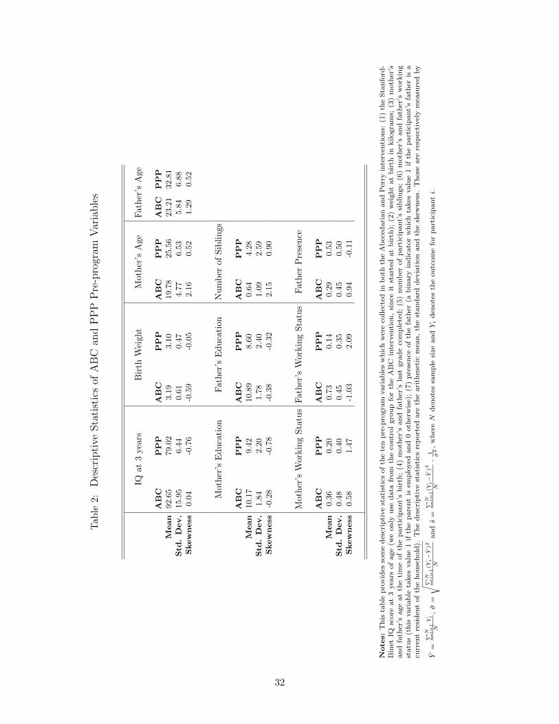
Tab

le2:

Descriptive

Statisticsof

ABC

andPPPPre-program

Variables

IQat

3ye

ars

Bir

thW

eight

Moth

er’s

Age

Fath

er’s

Age

ABC

PPP

ABC

PPP

ABC

PPP

ABC

PPP

Mean

92.6

579.0

23.1

93.1

019.7

825.5

623.2

132.8

1Std

.Dev.

15.9

56.4

40.6

10.4

74.7

76.5

35.8

46.8

8Skewness

0.0

4-0

.76

-0.5

9-0

.05

2.1

60.5

21.2

90.5

2

Mot

her

’sE

du

cati

on

Fath

er’s

Ed

uca

tion

Nu

mb

erof

Sib

lin

gs

ABC

PPP

ABC

PPP

ABC

PPP

Mean

10.1

79.4

210.8

98.6

00.6

44.2

8Std

.Dev.

1.8

42.2

01.7

82.4

01.0

92.5

9Skewness

-0.2

8-0

.78

-0.3

8-0

.32

2.1

50.9

0

Mot

her

’sW

ork

ing

Sta

tus

Fath

er’s

Work

ing

Sta

tus

Fath

erP

rese

nce

ABC

PPP

ABC

PPP

ABC

PPP

Mean

0.3

60.2

00.7

30.1

40.2

90.5

3Std

.Dev.

0.4

80.4

00.4

50.3

50.4

50.5

0Skewness

0.5

81.4

7-1

.03

2.0

90.9

4-0

.11

Note

s:T

his

tab

lep

rovid

esso

me

des

crip

tive

stati

stic

sof

the

ten

pre

-pro

gra

mvari

ab

les

wh

ich

wer

eco

llec

ted

inb

oth

the

Ab

eced

ari

an

an

dP

erry

inte

rven

tion

s:(1

)th

eS

tan

ford

-B

inet

IQsc

ore

at

3yea

rsof

age

(we

on

lyu

sed

ata

from

the

contr

ol

gro

up

for

the

AB

Cin

terv

enti

on

,si

nce

itst

art

edat

bir

th);

(2)

wei

ght

at

bir

thin

kilogra

ms;

(3)

moth

er’s

an

dfa

ther

’sage

at

the

tim

eof

the

part

icip

ant’

sb

irth

;(4

)m

oth

er’s

an

dfa

ther

’sla

stgra

de

com

ple

ted

;(5

)nu

mb

erof

part

icip

ant’

ssi

bli

ngs;

(6)

moth

er’s

an

dfa

ther

’sw

ork

ing

statu

s(t

his

vari

ab

leta

kes

valu

e1

ifth

ep

are

nt

isem

plo

yed

an

d0

oth

erw

ise)

;(7

)p

rese

nce

of

the

fath

er(a

bin

ary

ind

icato

rw

hic

hta

kes

valu

e1

ifth

ep

art

icip

ant’

sfa

ther

isa

curr

ent

resi

den

tof

the

hou

seh

old

).T

he

des

crip

tive

stati

stic

sre

port

edare

the

ari

thm

etic

mea

n,

the

stan

dard

dev

iati

on

an

dth

esk

ewn

ess.

Th

ose

are

resp

ecti

vel

ym

easu

red

by

Y=

∑ N i=

1Yi

N,σ

=

√ ∑N i=

1(Y

i−Y

)2

Nan

ds

=∑ N i

=1(Y

i−Y

)3

N·

1 σ3,

wh

ereN

den

ote

ssa

mp

lesi

zean

dYi

den

ote

sth

eou

tcom

efo

rp

art

icip

anti.

32

Figure 1: Comparison Between Pre-program Variables of ABC and PPP

A. IQ at 3 years B. Birth Weight

40 60 80 100 120 1400

0.01

0.02

0.03

0.04

0.05

0.06

0.07

Stanford−binet IQ at 3 y.o.

Den

sity

ABCPPP

0.5 1 1.5 2 2.5 3 3.5 4 4.5 50

0.1

0.2

0.3

0.4

0.5

0.6

0.7

0.8

Birth Weight (in kilograms)

Den

sity

ABCPPP

C. Mother’s Age D. Father’s Age

10 15 20 25 30 35 40 45 500

0.02

0.04

0.06

0.08

0.1

0.12

0.14

Mother’s Age

Den

sity

ABCPPP

10 15 20 25 30 35 40 45 50 550

0.01

0.02

0.03

0.04

0.05

0.06

0.07

0.08

0.09

0.1

Father’s Age

Den

sity

ABCPPP

Notes: These figures present the density estimation of four pre-program variables collected in both the Perry and Abecedarianinterventions. Panel A plots the Stanford-Binet IQ score at 3 years of age (we only use data for the control group for theABC intervention, since it started at birth). Panel B plots the weight at birth in kilograms. Panel C and D plot the mother’sand father’s age at the time of the participant’s birth. These estimates are based on a normal kernel function with optimalbandwidth for normal densities.

33

Fig

ure

2:

Com

par

ison

Bet

wee

nP

re-p

rogr

amV

aria

ble

sof

AB

Can

dP

PP

A.

Mot

her

’sE

du

cati

onB

.F

ath

er’s

Ed

uca

tion

C.

Nu

mb

erof

Sib

lin

gs

24

68

1012

1416

0

0.050.

1

0.150.

2

0.250.

3

0.350.

4

Mot

her’s

Las

t Gra

de C

ompl

eted

Distribution

A

BC

PP

P

24

68

1012

1416

180

0.1

0.2

0.3

0.4

0.5

0.6

0.7

Fat

her’s

Las

t Gra

de C

ompl

eted

Distribution

A

BC

PP

P

02

46

810

1214

0

0.1

0.2

0.3

0.4

0.5

0.6

0.7

0.8

0.9

Num

ber

of S

iblin

gs

Distribution

A

BC

PP

P

D.

Mot

her

’sW

orkin

gSta

tus

E.

Fath

er’s

Work

ing

Sta

tus

F.

Fath

er’s

Pre

sen

ce

01

0

0.1

0.2

0.3

0.4

0.5

0.6

0.7

0.8

Mot

her’s

Wor

king

Sta

tus

Distribution

A

BC

PP

P

01

0

0.1

0.2

0.3

0.4

0.5

0.6

0.7

0.8

0.9

Fat

her’s

Wor

king

Sta

tus

Distribution

A

BC

PP

P

01

0

0.1

0.2

0.3

0.4

0.5

0.6

0.7

0.8

Fat

her’s

Pre

senc

e

Distribution

A

BC

PP

P

Note

s:T

hes

efi

gu

res

pre

sent

esti

mate

sof

the

emp

iric

al

dis

trib

uti

on

sof

thre

eca

tegori

cal

an

dth

ree

bin

ary

vari

ab

les

coll

ecte

din

both

the

Per

ryan

dA

bec

edari

an

inte

rven

tion

s.A

llvari

ab

les

wer

eco

llec

ted

at

the

on

set

of

each

inte

rven

tion

.P

an

els

Aan

dB

:m

oth

er’s

an

dfa

ther

’sla

stgra

de

com

ple

ted

.P

an

elC

:th

enu

mb

erof

part

icip

ant’

ssi

blin

gs.

Pan

elD

an

dE

:m

oth

er’s

an

dfa

ther

’sw

ork

ing

statu

s(a

bin

ary

ind

icato

rw

hic

hta

kes

valu

e1

ifth

ep

are

nt

isem

plo

yed

an

d0

oth

erw

ise)

.P

an

elF

:p

rese

nce

of

the

fath

er(a

bin

ary

ind

icato

rw

hic

hta

kes

valu

e1

ifth

ep

art

icip

ant’

sfa

ther

isa

curr

ent

resi

den

tof

the

hou

seh

old

).

34

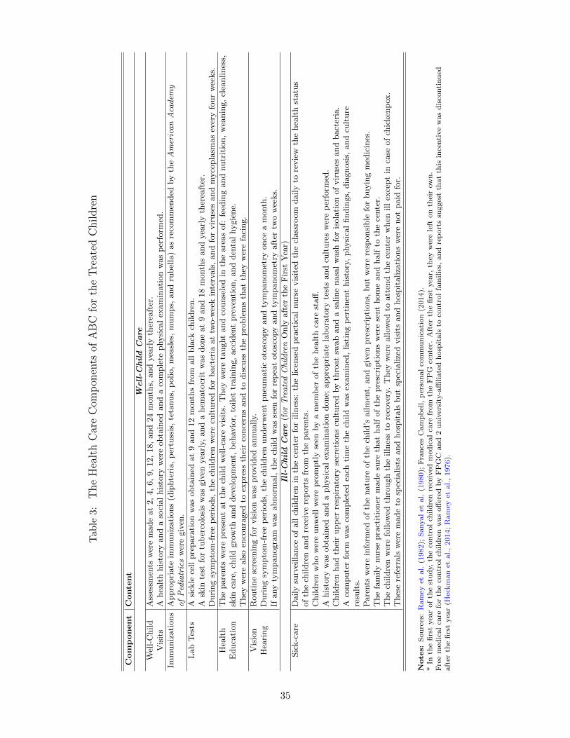
Tab

le3:TheHealthCareCom

pon

ents

ofABC

fortheTreated

Children

Component

Conte

nt

Well-C

hild

Care

Wel

l-C

hild

Ass

essm

ents

wer

em

ade

at

2,

4,

6,

9,

12,

18,

and

24

month

s,and

yea

rly

ther

eaft

er.

Vis

its

Ahea

lth

his

tory

and

aso

cial

his

tory

wer

eobta

ined

and

aco

mple

tephysi

cal

exam

inati

on

was

per

form

ed.

Imm

uniz

ati

ons

Appro

pri

ate

imm

uniz

ati

ons

(dip

hte

ria,

per

tuss

is,

teta

nus,

polio,

mea

sles

,m

um

ps,

and

rub

ella

)as

reco

mm

ended

by

theAmericanAcadem

yofPediatrics

wer

egiv

en.

Lab

Tes

tsA

sick

lece

llpre

para

tion

was

obta

ined

at

9and

12

month

sfr

om

all

bla

ckch

ildre

n.

Ask

inte

stfo

rtu

ber

colo

sis

was

giv

enyea

rly,

and

ahem

ato

crit

was

done

at

9and

18

month

sand

yea

rly

ther

eaft

er.

Duri

ng

sym

pto

m-f

ree

per

iods,

the

childre

nw

ere

cult

ure

dfo

rbact

eria

at

two-w

eek

inte

rvals

,and

for

vir

use

sand

myco

pla

smas

ever

yfo

ur

wee

ks.

Hea

lth

The

pare

nts

wer

epre

sent

at

the

child

wel

l-ca

revis

its.

They

wer

eta

ught

and

counse

led

inth

eare

as

of:

feed

ing

and

nutr

itio

n,

wea

nin

g,

clea

nlines

s,E

duca

tion

skin

care

,ch

ild

gro

wth

and

dev

elopm

ent,

beh

avio

r,to

ilet

train

ing,

acc

iden

tpre

ven

tion,

and

den

tal

hygie

ne.

They

wer

eals

oen

coura

ged

toex

pre

ssth

eir

conce

rns

and

todis

cuss

the

pro

ble

ms

that

they

wer

efa

cing.

Vis

ion

Routi

ne

scre

enin

gfo

rvis

ion

was

pro

vid

edannually.

Hea

ring

Duri

ng

sym

pto

m-f

ree

per

iods,

the

childre

nunder

wen

tpneu

mati

coto

scopy

and

tym

panom

etry

once

am

onth

.If

any

tym

panogra

mw

as

abnorm

al,

the

child

was

seen

for

rep

eat

oto

scopy

and

tym

panom

etry

aft

ertw

ow

eeks.

Ill-Child

Care

(forTreatedChildren

Only

aft

erth

eF

irst

Yea

r)

Sic

k-c

are

Daily

surv

eillance

of

all

childre

nin

the

cente

rfo

rilln

ess:

the

lice

nse

dpra

ctic

al

nurs

evis

ited

the

class

room

daily

tore

vie

wth

ehea

lth

statu

sof

the

childre

nand

rece

ive

rep

ort

sfr

om

the

pare

nts

.C

hildre

nw

ho

wer

eunw

ell

wer

epro

mptl

yse

enby

am

emb

erof

the

hea

lth

care

staff

.A

his

tory

was

obta

ined

and

aphysi

cal

exam

inati

on

done;

appro

pri

ate

lab

ora

tory

test

sand

cult

ure

sw

ere

per

form

ed.

Childre

nhad

thei

rupp

erre

spir

ato

ryse

cret

ions

cult

ure

dby

thro

at

swab

and

asa

line

nasa

lw

ash

for

isola

tion

of

vir

use

sand

bact

eria

.A

com

pute

rfo

rmw

as

com

ple

ted

each

tim

eth

ech

ild

was

exam

ined

,list

ing

per

tinen

this

tory

,physi

cal

findin

gs,

dia

gnosi

s,and

cult

ure

resu

lts.

Pare

nts

wer

ein

form

edof

the

natu

reof

the

child’s

ailm

ent,

and

giv

enpre

scri

pti

ons,

but

wer

ere

sponsi

ble

for

buyin

gm

edic

ines

.T

he

fam

ily

nurs

epra

ctit

ioner

made

sure

that

half

of

the

pre

scri

pti

ons

wer

ese

nt

hom

eand

half

toth

ece

nte

r.T

he

childre

nw

ere

follow

edth

rough

the

illn

ess

tore

cover

y.T

hey

wer

eallow

edto

att

end

the

cente

rw

hen

ill

exce

pt

inca

seof

chic

ken

pox

.T

hes

ere

ferr

als

wer

em

ade

tosp

ecia

list

sand

hosp

itals

but

spec

ialize

dvis

its

and

hosp

italiza

tions

wer

enot

paid

for.

Note

s:S

ou

rces

:R

am

eyet

al.

(1982);

Sanyal

etal.

(1980);

Fra

nce

sC

am

pb

ell,

per

son

al

com

mu

nic

ati

on

(2014).

*In

the

firs

tyea

rof

the

stud

y,th

eco

ntr

ol

chil

dre

nre

ceiv

edm

edic

al

care

from

the

FP

Gce

nte

r.A

fter

the

firs

tyea

r,th

eyw

ere

left

on

thei

row

n.

Fre

em

edic

al

care

for

the

contr

ol

chil

dre

nw

as

off

ered

by

FP

GC

an

d2

un

iver

sity

-affi

liate

dh

osp

itals

toco

ntr

ol

fam

ilie

s,an

dre

port

ssu

gges

tth

at

this

ince

nti

ve

was

dis

conti

nu

edaft

erth

efi

rst

yea

r(H

eckm

an

etal.,

2014;

Ram

eyet

al.,

1976).

35

Tab

le4:Com

parab

ilityof

Dataon

Outcom

esin

theABC

andPPPStudies

Ou

tcom

eA

ge

Age

Com

pa-

Note

sP

PP

AB

Crab

ilit

yPhysica

lHea

lth

Exce

llen

tor

ver

ygood

hea

lth

40

30

Hig

hS

am

e5-p

oin

tsc

ale

.H

ealt

hst

op

ped

from

work

ing

40

30

Med

ium

Diff

eren

tre

call

per

iod

(‘p

ast

15

yrs

’in

PP

P,

‘ever

’in

AB

C)

an

dre

fere

nce

per

iod

(‘a

wee

kor

more

’in

PP

P,

not

spec

ified

inA

BC

).W

eight

40

30

Hig

hS

elf-

rep

ort

edin

PP

P,

mea

sure

din

AB

C.

Hei

ght

40

30

Hig

hS

elf-

rep

ort

edin

PP

P,

mea

sure

din

AB

C.

BM

I40

30

Hig

hH

eight

an

dw

eight

are

self

-rep

ort

edin

PP

P,

mea

sure

din

AB

C.

Over

wei

ght

(BM

I≥25)

40

30

Hig

hH

eight

an

dw

eight

are

self

-rep

ort

edin

PP

P,

mea

sure

din

AB

C.

Ob

ese

(BM

I≥30)

40

30

Hig

hH

eight

an

dw

eight

are

self

-rep

ort

edin

PP

P,

mea

sure

din

AB

C.

Dia

stolic

blo

od

pre

ssu

ren

/a

mid

30s

Non

eO

nly

mea

sure

din

AB

C.

Syst

olic

blo

od

pre

ssu

ren

/a

mid

30s

Non

eO

nly

mea

sure

din

AB

C.

Hea

lth

Insu

rance

Hea

lth

care

cover

age

40

30

Med

ium

PP

Pre

fers

to‘h

ealt

hca

reco

ver

age’

,A

BC

to‘h

ealt

hin

sura

nce

’;th

eop

tion

sare

com

para

ble

.E

mp

loyer

-pro

vid

edor

bou

ght

40

30

Med

ium

PP

Pre

fers

to‘m

edic

al

care

cover

age’

,A

BC

to‘h

ealt

hin

sura

nce

’;th

eop

tion

sare

com

para

ble

.P

rovid

edin

pri

son

40

n/a

Non

eO

pti

on

not

availab

lein

AB

C.

Demand

forHea

lth

Care

Hosp

italize

d40

mid

30s

Med

ium

Diff

eren

tre

call

per

iod

(‘p

ast

12

mth

s’in

PP

P,

not

spec

ified

inA

BC

).S

ched

ule

dtr

eatm

ent

or

exam

40

30

Med

ium

PP

Pre

fers

to‘d

oct

or,

emer

gen

cyro

om

,or

clin

icfo

rsc

hed

ule

dtr

eatm

ent

or

exam

;A

BC

refe

rsto

‘exam

for

illn

ess

or

inju

ry’;

the

reca

llp

erio

dis

the

sam

e(1

2m

onth

s).

Lifestyles-Dietand

Physica

lActivity

Physi

cal

act

ivit

y40

21

Low

Diff

eren

tre

call

per

iod

(‘p

ast

month

’in

PP

P,

‘past

7d

ays’

inA

BC

);d

iffer

ent

refe

ren

ceti

me

(‘re

gu

larl

y’

inP

PP

,‘a

tle

ast

20

min

ute

s’in

AB

C);

diff

eren

tw

ord

ing

(‘any

physi

cal

act

ivit

ies’

inP

PP

,‘s

port

sact

ivit

ies

that

mad

eyou

swea

tan

db

reath

eh

ard

’in

AB

C);

the

vari

ab

les

are

con

stru

cted

follow

ing

CD

Cgu

idel

ines

.D

iet

&nu

trit

ion

40

21

Low

Diff

eren

tre

call

per

iod

(‘p

ast

15

yea

rs’

inP

PP

,‘y

este

rday’

inA

BC

);d

iffer

ent

word

ing

(‘ch

an

ges

ind

iet

for

hea

lth

reaso

n’

inP

PP

,‘n

um

ber

of

tim

esate

fru

it’

inA

BC

)..

Lifestyles-Smokin

gN

ever

smoker

40

30

Med

ium

Diff

eren

tw

ord

ing

(‘at

least

100

cigare

ttes

(=5

pack

s)’

inP

PP

,‘r

egu

lar

smokin

g’

inA

BC

).N

ot

ad

aily

smoker

27&

40

30

Med

ium

Diff

eren

tre

call

per

iod

(‘n

ow

’in

PP

P,

‘du

rin

gth

ep

ast

30

days’

inA

BC

).N

ot

ah

eavy

smoker

27&

40

30

Med

ium

Diff

eren

tre

call

per

iod

(‘n

ow

’in

PP

P,

‘du

rin

gth

ep

ast

30

days’

inA

BC

);d

iffer

ent

refe

ren

cesa

mp

le(‘

daily

smoker

’in

PP

P,

‘on

the

days

that

you

smoked

’in

AB

C).

Nu

mb

erof

cigare

ttes

per

day

27&

40

30

Med

ium

Diff

eren

tre

call

per

iod

(‘n

ow

’in

PP

P,

‘du

rin

gth

ep

ast

30

days’

inA

BC

);d

iffer

ent

refe

ren

cesa

mp

le(‘

daily

smoker

’in

PP

P,

‘on

the

days

that

you

smoked

’in

AB

C).

Note

:th

evari

ab

leis

conti

nu

ou

sin

PP

P,

ban

ded

inA

BC

.A

ge

of

on

set

of

smokin

gn

/a

21-3

0N

on

eO

nly

ask

edin

AB

C.

Lifestyles-Drinkin

gN

ot

afr

equ

ent

dri

nker

27

30

Med

ium

Diff

eren

tre

call

per

iod

(un

spec

ified

inP

PP

,‘d

uri

ng

the

past

30

days’

inA

BC

);d

iffer

ent

word

ing

(fre

qu

ency

inP

PP

,nu

mb

erof

days

inA

BC

).N

ot

afr

equ

ent

dri

nker

40

30

Hig

hS

am

ere

call

per

iod

(past

30

days)

,sa

me

word

ing

(nu

mb

erof

days)

.A

lcoh

ol

con

sum

pti

on

27

30

Med

ium

Diff

eren

tre

call

per

iod

(un

spec

ified

inP

PP

,‘d

uri

ng

the

past

30

days’

inA

BC

);d

iffer

ent

word

ing

(fre

qu

ency

inP

PP

,nu

mb

erof

days

inA

BC

).A

lcoh

ol

con

sum

pti

on

40

30

Hig

hS

am

ere

call

per

iod

(past

30

days)

,sa

me

word

ing

(nu

mb

erof

days)

.A

ge

of

on

set

of

dri

nkin

g<

17

n/a

21

Non

eO

nly

ask

edin

AB

C.

Note

s:T

his

tab

lere

port

sth

ele

vel

of

com

para

bilit

yof

the

ou

tcom

esin

the

AB

Can

dP

PP

.T

he

des

crip

tion

of

how

the

vari

ab

les

have

bee

nco

nst

ruct

edon

the

basi

sof

the

qu

esti

on

sask

edin

the

data

collec

tion

sca

rrie

dou

tat

the

diff

eren

tsw

eep

sis

rep

ort

edin

the

Ap

pen

dix

,S

ecti

on

2.

We

defi

ne

com

para

bilit

yas

‘hig

h’

wh

enth

equ

esti

on

sare

the

sam

e,an

dat

most

ther

eis

ad

iffer

ence

inth

eco

llec

tion

met

hod

(e.g

.w

eight)

.W

ed

efin

eco

mp

ara

bilit

yas

‘med

ium

’w

hen

ther

eis

ad

iffer

ence

inth

equ

esti

on

sask

ed,

eith

erin

the

reca

ll/re

fere

nce

per

iod

,or

inth

ew

ord

ing;

how

ever

,th

equ

esti

on

sre

fer

oth

erw

ise

toth

esa

me

con

stru

ct(e

.g.

daily

smokin

g).

We

defi

ne

com

para

bilit

yas

‘low

’w

hen

on

lyth

ed

om

ain

sth

evari

ab

les

bel

on

gto

are

the

sam

e(e

.g.

physi

cal

act

ivit

y),

bu

tth

ere

are

sign

ifica

nt

diff

eren

ces

inth

equ

esti

on

sw

ord

ing.

We

defi

ne

com

para

bilit

yas

‘non

e’w

hen

the

vari

ab

les

have

on

lyb

een

collec

ted

inon

eof

the

two

inte

rven

tion

s.

36

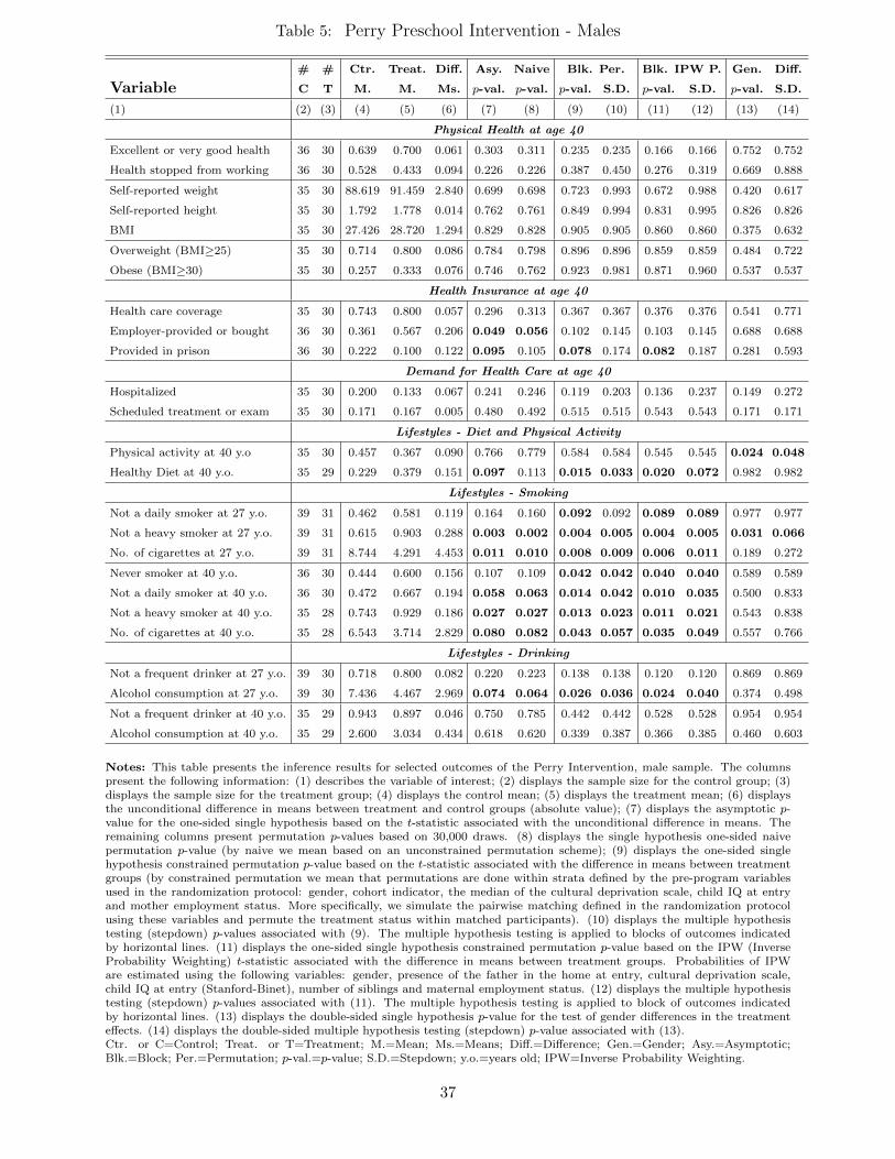
Table 5: Perry Preschool Intervention - Males

# # Ctr. Treat. Diff. Asy. Naive Blk. Per. Blk. IPW P. Gen. Diff.

Variable C T M. M. Ms. p-val. p-val. p-val. S.D. p-val. S.D. p-val. S.D.

(1) (2) (3) (4) (5) (6) (7) (8) (9) (10) (11) (12) (13) (14)

Physical Health at age 40

Excellent or very good health 36 30 0.639 0.700 0.061 0.303 0.311 0.235 0.235 0.166 0.166 0.752 0.752

Health stopped from working 36 30 0.528 0.433 0.094 0.226 0.226 0.387 0.450 0.276 0.319 0.669 0.888

Self-reported weight 35 30 88.619 91.459 2.840 0.699 0.698 0.723 0.993 0.672 0.988 0.420 0.617

Self-reported height 35 30 1.792 1.778 0.014 0.762 0.761 0.849 0.994 0.831 0.995 0.826 0.826

BMI 35 30 27.426 28.720 1.294 0.829 0.828 0.905 0.905 0.860 0.860 0.375 0.632

Overweight (BMI≥25) 35 30 0.714 0.800 0.086 0.784 0.798 0.896 0.896 0.859 0.859 0.484 0.722

Obese (BMI≥30) 35 30 0.257 0.333 0.076 0.746 0.762 0.923 0.981 0.871 0.960 0.537 0.537

Health Insurance at age 40

Health care coverage 35 30 0.743 0.800 0.057 0.296 0.313 0.367 0.367 0.376 0.376 0.541 0.771

Employer-provided or bought 36 30 0.361 0.567 0.206 0.049 0.056 0.102 0.145 0.103 0.145 0.688 0.688

Provided in prison 36 30 0.222 0.100 0.122 0.095 0.105 0.078 0.174 0.082 0.187 0.281 0.593

Demand for Health Care at age 40

Hospitalized 35 30 0.200 0.133 0.067 0.241 0.246 0.119 0.203 0.136 0.237 0.149 0.272

Scheduled treatment or exam 35 30 0.171 0.167 0.005 0.480 0.492 0.515 0.515 0.543 0.543 0.171 0.171

Lifestyles - Diet and Physical Activity

Physical activity at 40 y.o 35 30 0.457 0.367 0.090 0.766 0.779 0.584 0.584 0.545 0.545 0.024 0.048

Healthy Diet at 40 y.o. 35 29 0.229 0.379 0.151 0.097 0.113 0.015 0.033 0.020 0.072 0.982 0.982

Lifestyles - Smoking

Not a daily smoker at 27 y.o. 39 31 0.462 0.581 0.119 0.164 0.160 0.092 0.092 0.089 0.089 0.977 0.977

Not a heavy smoker at 27 y.o. 39 31 0.615 0.903 0.288 0.003 0.002 0.004 0.005 0.004 0.005 0.031 0.066

No. of cigarettes at 27 y.o. 39 31 8.744 4.291 4.453 0.011 0.010 0.008 0.009 0.006 0.011 0.189 0.272

Never smoker at 40 y.o. 36 30 0.444 0.600 0.156 0.107 0.109 0.042 0.042 0.040 0.040 0.589 0.589

Not a daily smoker at 40 y.o. 36 30 0.472 0.667 0.194 0.058 0.063 0.014 0.042 0.010 0.035 0.500 0.833

Not a heavy smoker at 40 y.o. 35 28 0.743 0.929 0.186 0.027 0.027 0.013 0.023 0.011 0.021 0.543 0.838

No. of cigarettes at 40 y.o. 35 28 6.543 3.714 2.829 0.080 0.082 0.043 0.057 0.035 0.049 0.557 0.766

Lifestyles - Drinking

Not a frequent drinker at 27 y.o. 39 30 0.718 0.800 0.082 0.220 0.223 0.138 0.138 0.120 0.120 0.869 0.869

Alcohol consumption at 27 y.o. 39 30 7.436 4.467 2.969 0.074 0.064 0.026 0.036 0.024 0.040 0.374 0.498

Not a frequent drinker at 40 y.o. 35 29 0.943 0.897 0.046 0.750 0.785 0.442 0.442 0.528 0.528 0.954 0.954

Alcohol consumption at 40 y.o. 35 29 2.600 3.034 0.434 0.618 0.620 0.339 0.387 0.366 0.385 0.460 0.603

Notes: This table presents the inference results for selected outcomes of the Perry Intervention, male sample. The columnspresent the following information: (1) describes the variable of interest; (2) displays the sample size for the control group; (3)displays the sample size for the treatment group; (4) displays the control mean; (5) displays the treatment mean; (6) displaysthe unconditional difference in means between treatment and control groups (absolute value); (7) displays the asymptotic p-value for the one-sided single hypothesis based on the t-statistic associated with the unconditional difference in means. Theremaining columns present permutation p-values based on 30,000 draws. (8) displays the single hypothesis one-sided naivepermutation p-value (by naive we mean based on an unconstrained permutation scheme); (9) displays the one-sided singlehypothesis constrained permutation p-value based on the t-statistic associated with the difference in means between treatmentgroups (by constrained permutation we mean that permutations are done within strata defined by the pre-program variablesused in the randomization protocol: gender, cohort indicator, the median of the cultural deprivation scale, child IQ at entryand mother employment status. More specifically, we simulate the pairwise matching defined in the randomization protocolusing these variables and permute the treatment status within matched participants). (10) displays the multiple hypothesistesting (stepdown) p-values associated with (9). The multiple hypothesis testing is applied to blocks of outcomes indicatedby horizontal lines. (11) displays the one-sided single hypothesis constrained permutation p-value based on the IPW (InverseProbability Weighting) t-statistic associated with the difference in means between treatment groups. Probabilities of IPWare estimated using the following variables: gender, presence of the father in the home at entry, cultural deprivation scale,child IQ at entry (Stanford-Binet), number of siblings and maternal employment status. (12) displays the multiple hypothesistesting (stepdown) p-values associated with (11). The multiple hypothesis testing is applied to block of outcomes indicatedby horizontal lines. (13) displays the double-sided single hypothesis p-value for the test of gender differences in the treatmenteffects. (14) displays the double-sided multiple hypothesis testing (stepdown) p-value associated with (13).Ctr. or C=Control; Treat. or T=Treatment; M.=Mean; Ms.=Means; Diff.=Difference; Gen.=Gender; Asy.=Asymptotic;Blk.=Block; Per.=Permutation; p-val.=p-value; S.D.=Stepdown; y.o.=years old; IPW=Inverse Probability Weighting.

37

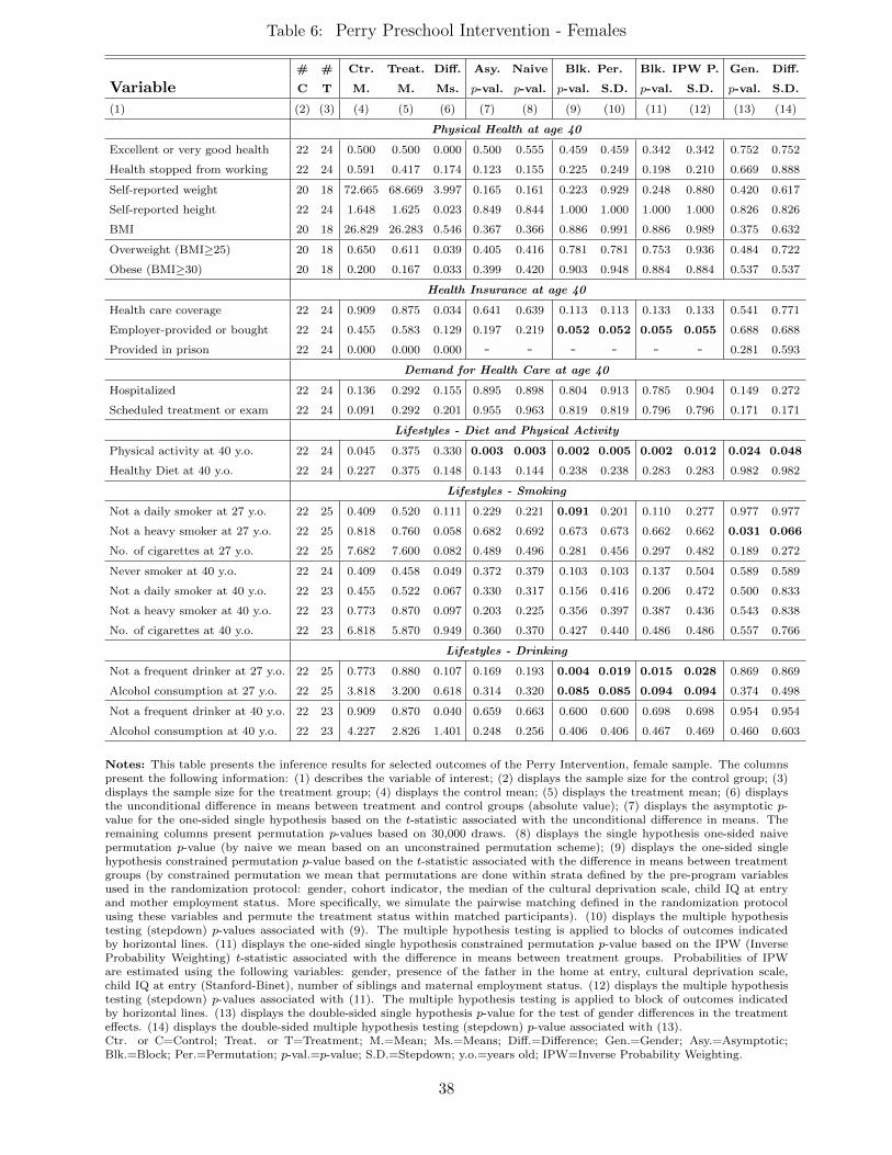
Table 6: Perry Preschool Intervention - Females

# # Ctr. Treat. Diff. Asy. Naive Blk. Per. Blk. IPW P. Gen. Diff.

Variable C T M. M. Ms. p-val. p-val. p-val. S.D. p-val. S.D. p-val. S.D.

(1) (2) (3) (4) (5) (6) (7) (8) (9) (10) (11) (12) (13) (14)

Physical Health at age 40

Excellent or very good health 22 24 0.500 0.500 0.000 0.500 0.555 0.459 0.459 0.342 0.342 0.752 0.752

Health stopped from working 22 24 0.591 0.417 0.174 0.123 0.155 0.225 0.249 0.198 0.210 0.669 0.888

Self-reported weight 20 18 72.665 68.669 3.997 0.165 0.161 0.223 0.929 0.248 0.880 0.420 0.617

Self-reported height 22 24 1.648 1.625 0.023 0.849 0.844 1.000 1.000 1.000 1.000 0.826 0.826

BMI 20 18 26.829 26.283 0.546 0.367 0.366 0.886 0.991 0.886 0.989 0.375 0.632

Overweight (BMI≥25) 20 18 0.650 0.611 0.039 0.405 0.416 0.781 0.781 0.753 0.936 0.484 0.722

Obese (BMI≥30) 20 18 0.200 0.167 0.033 0.399 0.420 0.903 0.948 0.884 0.884 0.537 0.537

Health Insurance at age 40

Health care coverage 22 24 0.909 0.875 0.034 0.641 0.639 0.113 0.113 0.133 0.133 0.541 0.771

Employer-provided or bought 22 24 0.455 0.583 0.129 0.197 0.219 0.052 0.052 0.055 0.055 0.688 0.688

Provided in prison 22 24 0.000 0.000 0.000 - - - - - - 0.281 0.593

Demand for Health Care at age 40

Hospitalized 22 24 0.136 0.292 0.155 0.895 0.898 0.804 0.913 0.785 0.904 0.149 0.272

Scheduled treatment or exam 22 24 0.091 0.292 0.201 0.955 0.963 0.819 0.819 0.796 0.796 0.171 0.171

Lifestyles - Diet and Physical Activity

Physical activity at 40 y.o. 22 24 0.045 0.375 0.330 0.003 0.003 0.002 0.005 0.002 0.012 0.024 0.048

Healthy Diet at 40 y.o. 22 24 0.227 0.375 0.148 0.143 0.144 0.238 0.238 0.283 0.283 0.982 0.982

Lifestyles - Smoking

Not a daily smoker at 27 y.o. 22 25 0.409 0.520 0.111 0.229 0.221 0.091 0.201 0.110 0.277 0.977 0.977

Not a heavy smoker at 27 y.o. 22 25 0.818 0.760 0.058 0.682 0.692 0.673 0.673 0.662 0.662 0.031 0.066

No. of cigarettes at 27 y.o. 22 25 7.682 7.600 0.082 0.489 0.496 0.281 0.456 0.297 0.482 0.189 0.272

Never smoker at 40 y.o. 22 24 0.409 0.458 0.049 0.372 0.379 0.103 0.103 0.137 0.504 0.589 0.589

Not a daily smoker at 40 y.o. 22 23 0.455 0.522 0.067 0.330 0.317 0.156 0.416 0.206 0.472 0.500 0.833

Not a heavy smoker at 40 y.o. 22 23 0.773 0.870 0.097 0.203 0.225 0.356 0.397 0.387 0.436 0.543 0.838

No. of cigarettes at 40 y.o. 22 23 6.818 5.870 0.949 0.360 0.370 0.427 0.440 0.486 0.486 0.557 0.766

Lifestyles - Drinking

Not a frequent drinker at 27 y.o. 22 25 0.773 0.880 0.107 0.169 0.193 0.004 0.019 0.015 0.028 0.869 0.869

Alcohol consumption at 27 y.o. 22 25 3.818 3.200 0.618 0.314 0.320 0.085 0.085 0.094 0.094 0.374 0.498

Not a frequent drinker at 40 y.o. 22 23 0.909 0.870 0.040 0.659 0.663 0.600 0.600 0.698 0.698 0.954 0.954

Alcohol consumption at 40 y.o. 22 23 4.227 2.826 1.401 0.248 0.256 0.406 0.406 0.467 0.469 0.460 0.603

Notes: This table presents the inference results for selected outcomes of the Perry Intervention, female sample. The columnspresent the following information: (1) describes the variable of interest; (2) displays the sample size for the control group; (3)displays the sample size for the treatment group; (4) displays the control mean; (5) displays the treatment mean; (6) displaysthe unconditional difference in means between treatment and control groups (absolute value); (7) displays the asymptotic p-value for the one-sided single hypothesis based on the t-statistic associated with the unconditional difference in means. Theremaining columns present permutation p-values based on 30,000 draws. (8) displays the single hypothesis one-sided naivepermutation p-value (by naive we mean based on an unconstrained permutation scheme); (9) displays the one-sided singlehypothesis constrained permutation p-value based on the t-statistic associated with the difference in means between treatmentgroups (by constrained permutation we mean that permutations are done within strata defined by the pre-program variablesused in the randomization protocol: gender, cohort indicator, the median of the cultural deprivation scale, child IQ at entryand mother employment status. More specifically, we simulate the pairwise matching defined in the randomization protocolusing these variables and permute the treatment status within matched participants). (10) displays the multiple hypothesistesting (stepdown) p-values associated with (9). The multiple hypothesis testing is applied to blocks of outcomes indicatedby horizontal lines. (11) displays the one-sided single hypothesis constrained permutation p-value based on the IPW (InverseProbability Weighting) t-statistic associated with the difference in means between treatment groups. Probabilities of IPWare estimated using the following variables: gender, presence of the father in the home at entry, cultural deprivation scale,child IQ at entry (Stanford-Binet), number of siblings and maternal employment status. (12) displays the multiple hypothesistesting (stepdown) p-values associated with (11). The multiple hypothesis testing is applied to block of outcomes indicatedby horizontal lines. (13) displays the double-sided single hypothesis p-value for the test of gender differences in the treatmenteffects. (14) displays the double-sided multiple hypothesis testing (stepdown) p-value associated with (13).Ctr. or C=Control; Treat. or T=Treatment; M.=Mean; Ms.=Means; Diff.=Difference; Gen.=Gender; Asy.=Asymptotic;Blk.=Block; Per.=Permutation; p-val.=p-value; S.D.=Stepdown; y.o.=years old; IPW=Inverse Probability Weighting.

38

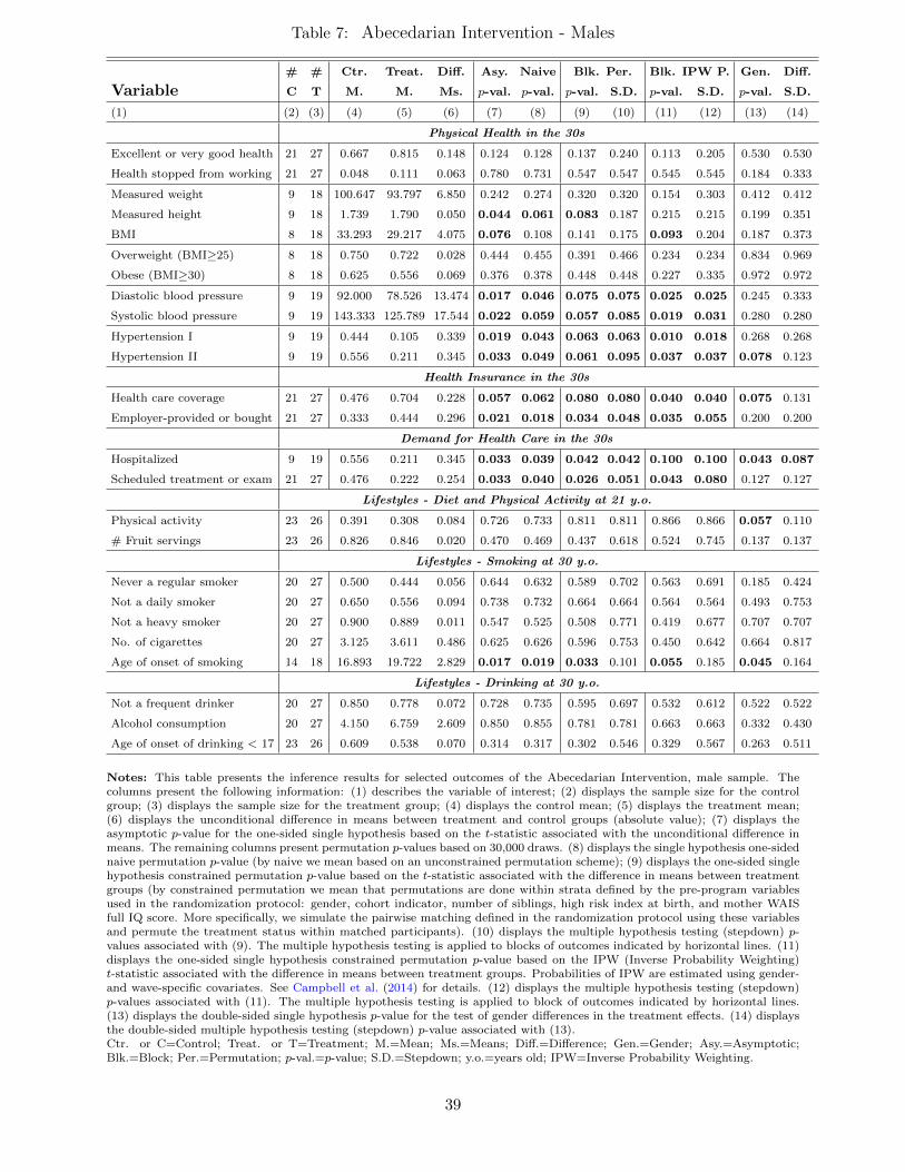
Table 7: Abecedarian Intervention - Males

# # Ctr. Treat. Diff. Asy. Naive Blk. Per. Blk. IPW P. Gen. Diff.

Variable C T M. M. Ms. p-val. p-val. p-val. S.D. p-val. S.D. p-val. S.D.

(1) (2) (3) (4) (5) (6) (7) (8) (9) (10) (11) (12) (13) (14)

Physical Health in the 30s

Excellent or very good health 21 27 0.667 0.815 0.148 0.124 0.128 0.137 0.240 0.113 0.205 0.530 0.530

Health stopped from working 21 27 0.048 0.111 0.063 0.780 0.731 0.547 0.547 0.545 0.545 0.184 0.333

Measured weight 9 18 100.647 93.797 6.850 0.242 0.274 0.320 0.320 0.154 0.303 0.412 0.412

Measured height 9 18 1.739 1.790 0.050 0.044 0.061 0.083 0.187 0.215 0.215 0.199 0.351

BMI 8 18 33.293 29.217 4.075 0.076 0.108 0.141 0.175 0.093 0.204 0.187 0.373

Overweight (BMI≥25) 8 18 0.750 0.722 0.028 0.444 0.455 0.391 0.466 0.234 0.234 0.834 0.969

Obese (BMI≥30) 8 18 0.625 0.556 0.069 0.376 0.378 0.448 0.448 0.227 0.335 0.972 0.972

Diastolic blood pressure 9 19 92.000 78.526 13.474 0.017 0.046 0.075 0.075 0.025 0.025 0.245 0.333

Systolic blood pressure 9 19 143.333 125.789 17.544 0.022 0.059 0.057 0.085 0.019 0.031 0.280 0.280

Hypertension I 9 19 0.444 0.105 0.339 0.019 0.043 0.063 0.063 0.010 0.018 0.268 0.268

Hypertension II 9 19 0.556 0.211 0.345 0.033 0.049 0.061 0.095 0.037 0.037 0.078 0.123

Health Insurance in the 30s

Health care coverage 21 27 0.476 0.704 0.228 0.057 0.062 0.080 0.080 0.040 0.040 0.075 0.131

Employer-provided or bought 21 27 0.333 0.444 0.296 0.021 0.018 0.034 0.048 0.035 0.055 0.200 0.200

Demand for Health Care in the 30s

Hospitalized 9 19 0.556 0.211 0.345 0.033 0.039 0.042 0.042 0.100 0.100 0.043 0.087

Scheduled treatment or exam 21 27 0.476 0.222 0.254 0.033 0.040 0.026 0.051 0.043 0.080 0.127 0.127

Lifestyles - Diet and Physical Activity at 21 y.o.

Physical activity 23 26 0.391 0.308 0.084 0.726 0.733 0.811 0.811 0.866 0.866 0.057 0.110

# Fruit servings 23 26 0.826 0.846 0.020 0.470 0.469 0.437 0.618 0.524 0.745 0.137 0.137

Lifestyles - Smoking at 30 y.o.

Never a regular smoker 20 27 0.500 0.444 0.056 0.644 0.632 0.589 0.702 0.563 0.691 0.185 0.424

Not a daily smoker 20 27 0.650 0.556 0.094 0.738 0.732 0.664 0.664 0.564 0.564 0.493 0.753

Not a heavy smoker 20 27 0.900 0.889 0.011 0.547 0.525 0.508 0.771 0.419 0.677 0.707 0.707

No. of cigarettes 20 27 3.125 3.611 0.486 0.625 0.626 0.596 0.753 0.450 0.642 0.664 0.817

Age of onset of smoking 14 18 16.893 19.722 2.829 0.017 0.019 0.033 0.101 0.055 0.185 0.045 0.164

Lifestyles - Drinking at 30 y.o.

Not a frequent drinker 20 27 0.850 0.778 0.072 0.728 0.735 0.595 0.697 0.532 0.612 0.522 0.522

Alcohol consumption 20 27 4.150 6.759 2.609 0.850 0.855 0.781 0.781 0.663 0.663 0.332 0.430

Age of onset of drinking < 17 23 26 0.609 0.538 0.070 0.314 0.317 0.302 0.546 0.329 0.567 0.263 0.511

Notes: This table presents the inference results for selected outcomes of the Abecedarian Intervention, male sample. Thecolumns present the following information: (1) describes the variable of interest; (2) displays the sample size for the controlgroup; (3) displays the sample size for the treatment group; (4) displays the control mean; (5) displays the treatment mean;(6) displays the unconditional difference in means between treatment and control groups (absolute value); (7) displays theasymptotic p-value for the one-sided single hypothesis based on the t-statistic associated with the unconditional difference inmeans. The remaining columns present permutation p-values based on 30,000 draws. (8) displays the single hypothesis one-sidednaive permutation p-value (by naive we mean based on an unconstrained permutation scheme); (9) displays the one-sided singlehypothesis constrained permutation p-value based on the t-statistic associated with the difference in means between treatmentgroups (by constrained permutation we mean that permutations are done within strata defined by the pre-program variablesused in the randomization protocol: gender, cohort indicator, number of siblings, high risk index at birth, and mother WAISfull IQ score. More specifically, we simulate the pairwise matching defined in the randomization protocol using these variablesand permute the treatment status within matched participants). (10) displays the multiple hypothesis testing (stepdown) p-values associated with (9). The multiple hypothesis testing is applied to blocks of outcomes indicated by horizontal lines. (11)displays the one-sided single hypothesis constrained permutation p-value based on the IPW (Inverse Probability Weighting)t-statistic associated with the difference in means between treatment groups. Probabilities of IPW are estimated using gender-and wave-specific covariates. See Campbell et al. (2014) for details. (12) displays the multiple hypothesis testing (stepdown)p-values associated with (11). The multiple hypothesis testing is applied to block of outcomes indicated by horizontal lines.(13) displays the double-sided single hypothesis p-value for the test of gender differences in the treatment effects. (14) displaysthe double-sided multiple hypothesis testing (stepdown) p-value associated with (13).Ctr. or C=Control; Treat. or T=Treatment; M.=Mean; Ms.=Means; Diff.=Difference; Gen.=Gender; Asy.=Asymptotic;Blk.=Block; Per.=Permutation; p-val.=p-value; S.D.=Stepdown; y.o.=years old; IPW=Inverse Probability Weighting.

39

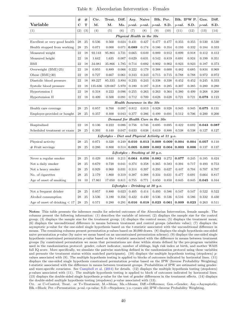
Table 8: Abecedarian Intervention - Females

# # Ctr. Treat. Diff. Asy. Naive Blk. Per. Blk. IPW P. Gen. Diff.

Variable C T M. M. Ms. p-val. p-val. p-val. S.D. p-val. S.D. p-val. S.D.

(1) (2) (3) (4) (5) (6) (7) (8) (9) (10) (11) (12) (13) (14)

Physical Health in the 30s

Excellent or very good health 28 25 0.536 0.560 0.024 0.431 0.427 0.477 0.477 0.355 0.355 0.530 0.530

Health stopped from working 28 25 0.071 0.000 0.071 0.089 0.174 0.186 0.354 0.193 0.332 0.184 0.333

Measured weight 22 18 92.143 95.864 3.721 0.665 0.649 0.889 0.912 0.899 0.918 0.412 0.412

Measured height 22 18 1.642 1.635 0.007 0.629 0.631 0.542 0.819 0.691 0.924 0.199 0.351

BMI 22 18 34.081 35.866 1.785 0.714 0.692 0.902 0.902 0.923 0.923 0.187 0.373

Overweight (BMI≥25) 22 18 0.955 0.889 0.066 0.222 0.179 0.388 0.600 0.482 0.685 0.834 0.969

Obese (BMI≥30) 22 18 0.727 0.667 0.061 0.343 0.343 0.715 0.715 0.788 0.788 0.972 0.972

Diastolic blood pressure 22 18 89.227 85.333 3.894 0.233 0.243 0.338 0.338 0.452 0.452 0.245 0.333

Systolic blood pressure 22 18 135.636 129.667 5.970 0.180 0.187 0.218 0.285 0.307 0.385 0.280 0.280

Hypertension I 22 18 0.318 0.222 0.096 0.255 0.263 0.263 0.364 0.380 0.499 0.268 0.268

Hypertension II 22 18 0.409 0.500 0.091 0.712 0.709 0.628 0.628 0.721 0.721 0.078 0.123

Health Insurance in the 30s

Health care coverage 28 25 0.857 0.760 0.097 0.812 0.813 0.928 0.928 0.945 0.945 0.075 0.131

Employer-provided or bought 28 25 0.357 0.400 0.043 0.377 0.386 0.499 0.691 0.512 0.706 0.200 0.200

Demand for Health Care in the 30s

Hospitalized 22 18 0.136 0.222 0.086 0.756 0.746 0.695 0.695 0.422 0.692 0.043 0.087

Scheduled treatment or exam 28 25 0.393 0.440 0.047 0.633 0.638 0.619 0.888 0.538 0.538 0.127 0.127

Lifestyles - Diet and Physical Activity at 21 y.o.

Physical activity 28 25 0.071 0.320 0.249 0.010 0.013 0.009 0.009 0.004 0.004 0.057 0.110

# Fruit servings 28 25 0.286 0.800 0.514 0.005 0.009 0.002 0.004 0.003 0.006 0.137 0.137

Lifestyles - Smoking at 30 y.o.

Never a regular smoker 28 25 0.429 0.640 0.211 0.064 0.056 0.082 0.272 0.077 0.245 0.185 0.424

Not a daily smoker 28 25 0.679 0.720 0.041 0.374 0.358 0.365 0.583 0.394 0.717 0.493 0.753

Not a heavy smoker 28 25 0.929 0.960 0.031 0.314 0.397 0.293 0.627 0.447 0.704 0.707 0.707

No. of cigarettes 28 25 2.179 1.860 0.319 0.387 0.388 0.334 0.631 0.477 0.691 0.664 0.817

Age of onset of smoking 18 10 17.861 17.050 0.811 0.755 0.771 0.850 0.850 0.845 0.845 0.045 0.164

Lifestyles - Drinking at 30 y.o.

Not a frequent drinker 28 25 0.857 0.880 0.023 0.405 0.414 0.493 0.586 0.547 0.547 0.522 0.522

Alcohol consumption 28 25 3.536 3.180 0.356 0.422 0.430 0.536 0.536 0.516 0.586 0.332 0.430

Age of onset of drinking < 17 28 25 0.571 0.280 0.291 0.016 0.018 0.023 0.061 0.009 0.023 0.263 0.511

Notes: This table presents the inference results for selected outcomes of the Abecedarian Intervention, female sample. Thecolumns present the following information: (1) describes the variable of interest; (2) displays the sample size for the controlgroup; (3) displays the sample size for the treatment group; (4) displays the control mean; (5) displays the treatment mean;(6) displays the unconditional difference in means between treatment and control groups (absolute value); (7) displays theasymptotic p-value for the one-sided single hypothesis based on the t-statistic associated with the unconditional difference inmeans. The remaining columns present permutation p-values based on 30,000 draws. (8) displays the single hypothesis one-sidednaive permutation p-value (by naive we mean based on an unconstrained permutation scheme); (9) displays the one-sided singlehypothesis constrained permutation p-value based on the t-statistic associated with the difference in means between treatmentgroups (by constrained permutation we mean that permutations are done within strata defined by the pre-program variablesused in the randomization protocol: gender, cohort indicator, number of siblings, high risk index at birth, and mother WAISfull IQ score. More specifically, we simulate the pairwise matching defined in the randomization protocol using these variablesand permute the treatment status within matched participants). (10) displays the multiple hypothesis testing (stepdown) p-values associated with (9). The multiple hypothesis testing is applied to blocks of outcomes indicated by horizontal lines. (11)displays the one-sided single hypothesis constrained permutation p-value based on the IPW (Inverse Probability Weighting)t-statistic associated with the difference in means between treatment groups. Probabilities of IPW are estimated using gender-and wave-specific covariates. See Campbell et al. (2014) for details. (12) displays the multiple hypothesis testing (stepdown)p-values associated with (11). The multiple hypothesis testing is applied to block of outcomes indicated by horizontal lines.(13) displays the double-sided single hypothesis p-value for the test of gender differences in the treatment effects. (14) displaysthe double-sided multiple hypothesis testing (stepdown) p-value associated with (13).Ctr. or C=Control; Treat. or T=Treatment; M.=Mean; Ms.=Means; Diff.=Difference; Gen.=Gender; Asy.=Asymptotic;Blk.=Block; Per.=Permutation; p-val.=p-value; S.D.=Stepdown; y.o.=years old; IPW=Inverse Probability Weighting.

40

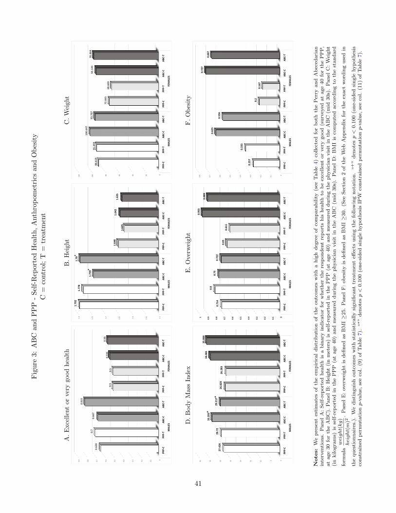
Fig

ure

3:A

BC

and

PP

P-

Sel

f-R

epor

ted

Hea

lth

,A

nth

rop

omet

rics

and

Ob

esit

yC

=co

ntr

ol;

T=

trea

tmen

t

A.

Exce

llen

tor

very

good

hea

lth

B.

Hei

ght

C.

Wei

ght

0

0.1

0.2

0.3

0.4

0.5

0.6

0.7

0.8

0.9

PPP‐C

PPP‐T

ABC‐C

ABC‐T

PPP‐C

PPP‐T

ABC‐C

ABC‐T

MAL

ESFEMAL

ES

0.639

0.7

0.667

0.815

0.5

0.5

0.536

0.56

1.5

1.551.6

1.651.7

1.751.8

PPP‐C

PPP‐T

ABC‐C

ABC‐T

PPP‐C

PPP‐T

ABC‐C

ABC‐T

MAL

ESFEMAL

ES

1.792

1.778

1.739+

1.79+

1.648

1.625

1.642

1.635

020406080100

120

PPP‐C

PPP‐T

ABC‐C

ABC‐T

PPP‐C

PPP‐T

ABC‐C

ABC‐T

MAL

ESFEMAL

ES

88.619

91.459

100.647

93.797

72.665

68.669

92.143

95.864

D.

Bod

yM

ass

Ind

exE

.O

ver

wei

ght

F.

Ob

esit

y

0510152025303540

PPP‐C

PPP‐T

ABC‐C

ABC‐T

PPP‐C

PPP‐T

ABC‐C

ABC‐T

MAL

ESFEMAL

ES

27.426

28.72

33.293*

29.217*

26.829

26.283

34.081

35.866

0

0.1

0.2

0.3

0.4

0.5

0.6

0.7

0.8

0.91

PPP‐C

PPP‐T

ABC‐C

ABC‐T

PPP‐C

PPP‐T

ABC‐C

ABC‐T

MAL

ESFEMAL

ES

0.714

0.8

0.75

0.722

0.65

0.611

0.955

0.889

0

0.1

0.2

0.3

0.4

0.5

0.6

0.7

0.8

PPP‐C

PPP‐T

ABC‐C

ABC‐T

PPP‐C

PPP‐T

ABC‐C

ABC‐T

MAL

ESFEMAL

ES

0.257

0.333

0.625

0.556

0.2

0.167

0.727

0.667

Note

s:W

ep

rese

nt

esti

mate

sof

the

emp

iric

al

dis

trib

uti

on

of

the

ou

tcom

esw

ith

ah

igh

deg

ree

of

com

para

bilit

y(s

eeT

ab

le4)

collec

ted

for

both

the

Per

ryan

dA

bec

edari

an

inte

rven

tion

s.P

an

elA

:S

elf-

rep

ort

edh

ealt

his

ab

inary

ind

icato

rfo

rw

het

her

the

resp

on

den

tre

port

sh

ish

ealt

hto

be

exce

llen

tor

ver

ygood

(su

rvey

edat

age

40

for

the

PP

P,

at

age

30

for

the

AB

C).

Pan

elB

:H

eight

(in

met

ers)

isse

lf-r

eport

edin

the

PP

P(a

tage

40)

an

dm

easu

red

du

rin

gth

ep

hysi

cian

vis

itin

the

AB

C(m

id30s)

.P

an

elC

:W

eight

(in

kilogra

ms)

isse

lf-r

eport

edin

the

PP

P(a

tage

40)

an

dm

easu

red

du

rin

gth

ep

hysi

cian

vis

itin

the

AB

C(m

id30s)

.P

an

elD

:B

MI

isco

mp

ute

dacc

ord

ing

toth

est

an

dard

form

ula

weight(kg)

height(m

)2.

Pan

elE

:over

wei

ght

isd

efin

edas

BM

I≥

25.

Pan

elF

:ob

esit

yis

defi

ned

as

BM

I≥

30.

(See

Sec

tion

2of

the

Web

Ap

pen

dix

for

the

exact

word

ing

use

din

the

qu

esti

on

nair

es.)

.W

ed

isti

ngu

ish

ou

tcom

esw

ith

stati

stic

ally

sign

ifica

nt

trea

tmen

teff

ects

usi

ng

the

follow

ing

nota

tion

.“

+”

den

ote

sp<

0.1

00

(on

e-si

ded

sin

gle

hyp

oth

esis

con

stra

ined

per

mu

tati

onp-v

alu

e,se

eco

l.(9

)of

Tab

le7).

“∗”

den

ote

sp<

0.1

00

(on

e-si

ded

sin

gle

hyp

oth

esis

IPW

con

stra

ined

per

mu

tati

onp-v

alu

e,se

eco

l.(1

1)

of

Tab

le7).

41

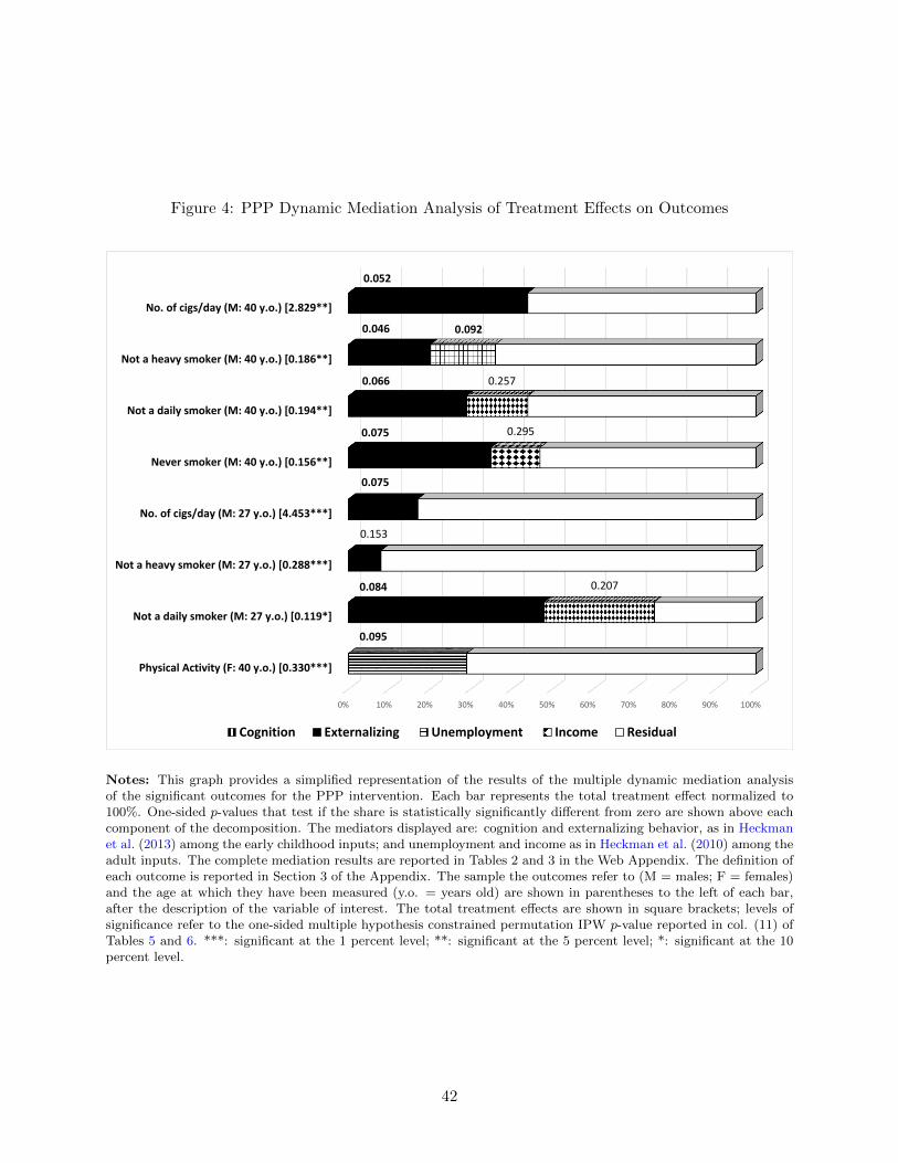
Figure 4: PPP Dynamic Mediation Analysis of Treatment Effects on Outcomes

0% 10% 20% 30% 40% 50% 60% 70% 80% 90% 100%

Physical Activity (F: 40 y.o.) [0.330***]

Not a daily smoker (M: 27 y.o.) [0.119*]

Not a heavy smoker (M: 27 y.o.) [0.288***]

No. of cigs/day (M: 27 y.o.) [4.453***]

Never smoker (M: 40 y.o.) [0.156**]

Not a daily smoker (M: 40 y.o.) [0.194**]

Not a heavy smoker (M: 40 y.o.) [0.186**]

No. of cigs/day (M: 40 y.o.) [2.829**]

Cognition Externalizing Unemployment Income Residual

0.052

0.046

0.066

0.075

0.075

0.153

0.084

0.095

0.207

0.295

0.257

0.092

Notes: This graph provides a simplified representation of the results of the multiple dynamic mediation analysisof the significant outcomes for the PPP intervention. Each bar represents the total treatment effect normalized to100%. One-sided p-values that test if the share is statistically significantly different from zero are shown above eachcomponent of the decomposition. The mediators displayed are: cognition and externalizing behavior, as in Heckmanet al. (2013) among the early childhood inputs; and unemployment and income as in Heckman et al. (2010) among theadult inputs. The complete mediation results are reported in Tables 2 and 3 in the Web Appendix. The definition ofeach outcome is reported in Section 3 of the Appendix. The sample the outcomes refer to (M = males; F = females)and the age at which they have been measured (y.o. = years old) are shown in parentheses to the left of each bar,after the description of the variable of interest. The total treatment effects are shown in square brackets; levels ofsignificance refer to the one-sided multiple hypothesis constrained permutation IPW p-value reported in col. (11) ofTables 5 and 6. ***: significant at the 1 percent level; **: significant at the 5 percent level; *: significant at the 10percent level.

42

Figure 5: PPP: Static versus Dynamic Mediation Analysis of Treatment Effects on Outcomes

(a) Early Child Development Mediators

0 10 20 30 40 50 60

Physical Activity (F: 40 y.o.)

Not a daily smoker (M: 27 y.o.)

Not a heavy smoker (M: 27 y.o.)

No. of cigs/day (M: 27 y.o.)

Never smoker (M: 40 y.o.)

Not a daily smoker (M: 40 y.o.)

Not a heavy smoker (M: 40 y.o.)

No. of cigs/day (M: 40 y.o.)

Externalizing‐S Externalizing‐D Cognition‐S Cognition‐D

(b) Adult Socioeconomic Status Mediators

0 10 20 30 40 50 60 70 80 90

Not a daily smoker (M: 27 y.o.)

Not a heavy smoker (M: 27 y.o.)

No. of cigs/day (M: 27 y.o.)

Never smoker (M: 40 y.o.)

Not a daily smoker (M: 40 y.o.)

Not a heavy smoker (M: 40 y.o.)

No. of cigs/day (M: 40 y.o.)

Income‐S Income‐D Unemployment‐S Unemployment‐D

Notes: This figure is comprised of two panels. Each panel provides a simplified representation of the results ofthe static and of the dynamic mediation analyses of the significant outcomes for the PPP intervention, respectivelyby comparing the results for the early child development mediators cognition and externalizing behavior (panel (a))and for the adult socioeconomic inputs unemployment and income (panel (b)). For each outcome and mediator, thelighter-colored bars display the static mediation analysis results, while the darker-colored bars display the dynamicmediation analysis results (as shown in Figure 4). The complete mediation results are reported in Tables 2, 3 and 4in the Web Appendix. The definition of each outcome is reported in Section 3 of the Web Appendix. The samplethe outcomes refer to (M = males; F = females) and the age at which they have been measured (y.o. = years old)are shown in parentheses to the left of each bar, after the description of the variable of interest. S=static mediationanalysis; D=dynamic mediation analysis. 43

Figure 6: ABC Dynamic Mediation Analysis of Treatment Effects on Outcomes

0% 10% 20% 30% 40% 50% 60% 70% 80% 90% 100%

HI coverage (M: 30 y.o.) [0.228**]

HI by the employer (M: 30 y.o.) [0.296**]

Hypertension I (M: 35 y.o.) [0.339***]

Hypertension II (M: 35 y.o.) [0.345**]

Diastolic blood pressure (M: 35 y.o.) [13.474**]

Systolic blood pressure (M: 35 y.o.) [17.544**]

Task Orientation BMI Employment BMI‐Employment Residual

0.092 0.095

0.081 0.049

0.083 0.147

0.076 0.078

0.100 0.179

0.163 0.203

Notes: This graph provides a simplified representation of the results of the multiple dynamic mediation analysisof the significant outcomes for the ABC intervention. Each bar represents the total treatment effect normalized to100%. One-sided p-values that test if the share is statistically significantly different from zero are shown above eachcomponent of the decomposition. The mediators displayed are: task orientation as in Burchinal et al. (1997) andBMI as in Campbell et al. (2014) among the early childhood inputs; and employment as in Garcia et al. (2014) amongthe adult inputs. The complete mediation results are reported in Table 5 in the Web Appendix. The definition ofeach outcome is reported in Section 3 of the Web Appendix. The sample the outcomes refer to (M = males) andthe age at which they have been measured (y.o. = years old) are shown in parentheses to the left of each bar, afterthe description of the variable of interest (HI=Health Insurance). The total treatment effects are shown in squarebrackets. Levels of significance refer to the one-sided multiple hypothesis constrained permutation IPW p-valuereported in col. (11) of Table 7. ***: significant at the 1 percent level; **: significant at the 5 percent level; *:significant at the 10 percent level.

44

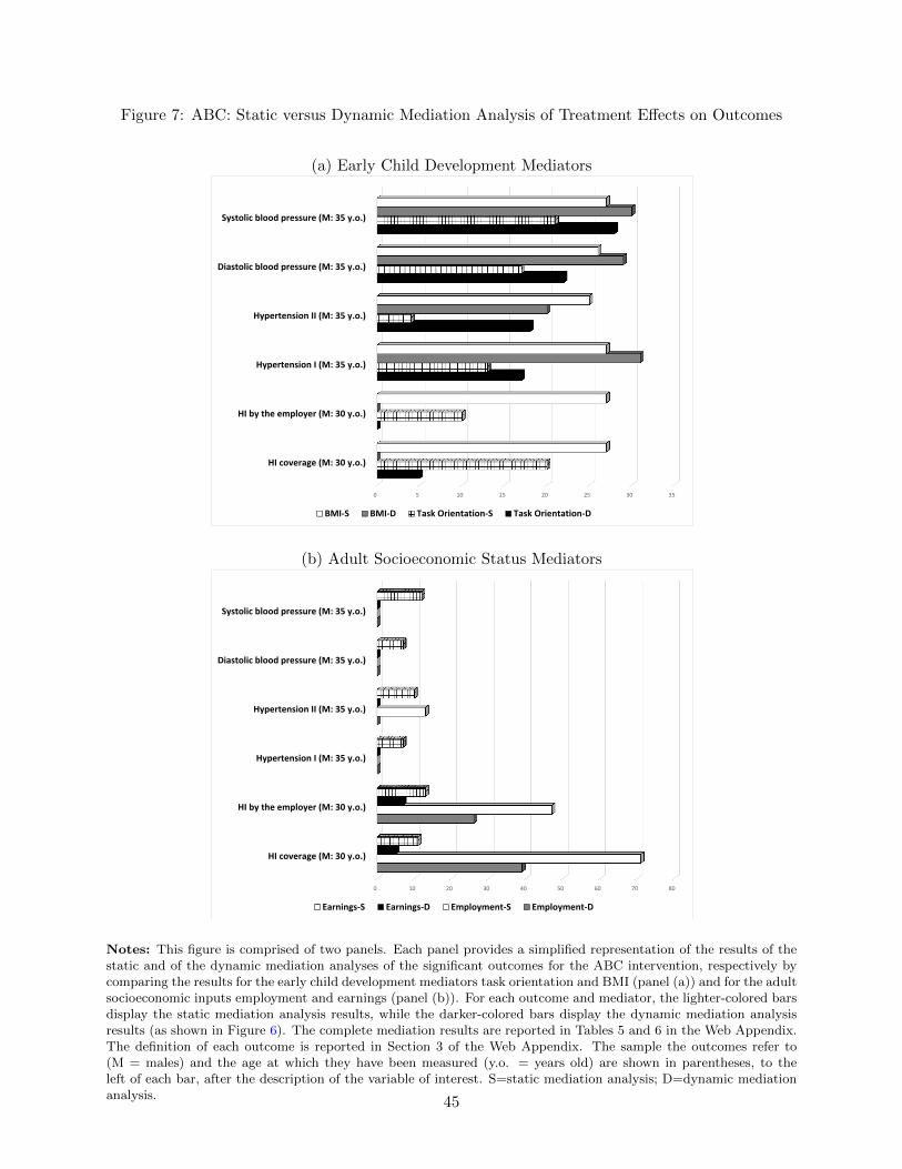
Figure 7: ABC: Static versus Dynamic Mediation Analysis of Treatment Effects on Outcomes

(a) Early Child Development Mediators

0 5 10 15 20 25 30 35

HI coverage (M: 30 y.o.)

HI by the employer (M: 30 y.o.)

Hypertension I (M: 35 y.o.)

Hypertension II (M: 35 y.o.)

Diastolic blood pressure (M: 35 y.o.)

Systolic blood pressure (M: 35 y.o.)

BMI‐S BMI‐D Task Orientation‐S Task Orientation‐D

(b) Adult Socioeconomic Status Mediators

0 10 20 30 40 50 60 70 80

HI coverage (M: 30 y.o.)

HI by the employer (M: 30 y.o.)

Hypertension I (M: 35 y.o.)

Hypertension II (M: 35 y.o.)

Diastolic blood pressure (M: 35 y.o.)

Systolic blood pressure (M: 35 y.o.)

Earnings‐S Earnings‐D Employment‐S Employment‐D

Notes: This figure is comprised of two panels. Each panel provides a simplified representation of the results of thestatic and of the dynamic mediation analyses of the significant outcomes for the ABC intervention, respectively bycomparing the results for the early child development mediators task orientation and BMI (panel (a)) and for the adultsocioeconomic inputs employment and earnings (panel (b)). For each outcome and mediator, the lighter-colored barsdisplay the static mediation analysis results, while the darker-colored bars display the dynamic mediation analysisresults (as shown in Figure 6). The complete mediation results are reported in Tables 5 and 6 in the Web Appendix.The definition of each outcome is reported in Section 3 of the Web Appendix. The sample the outcomes refer to(M = males) and the age at which they have been measured (y.o. = years old) are shown in parentheses, to theleft of each bar, after the description of the variable of interest. S=static mediation analysis; D=dynamic mediationanalysis. 45

References

Akaike, H. (1974, December). A new look at the statistical model identification. IEEE Transactions

on Automatic Control 19 (6), 716–723.

Bagchi, D. and H. G. Preuss (2012). Obesity: Epidemiology, pathophysiology, and prevention. CRC

Press.

Barnett, W. S. and L. N. Masse (2007, February). Comparative benefit-cost analysis of the

Abecedarian program and its policy implications. Economics of Education Review 26 (1), 113–

125.

Bjornson, W., C. Rand, J. E. Connett, P. Lindgren, M. Nides, F. Pope, A. S. Buist, C. Hoppe-Ryan,

and P. O’Hara (1995). Gender differences in smoking cessation after 3 years in the lung health

study. American Journal of Public Health 85 (2), 223–230.

Black, M. M. and K. M. Hurley (2014). Investment in early childhood development. The Lancet .

Boyd, M. P., C. Weinmann, Z. Yin, et al. (2002). The relationship of physical self-perceptions and

goal orientations to intrinsic motivation for exercise. Journal of Sport Behavior 25 (1), 1–18.

Burchinal, M. R., F. A. Campbell, D. M. Brayant, B. H. Wasik, and C. T. Ramey (1997). Early

intervention and mediating processes in cognitive performance of children of low-income african

american families. Child Development 68 (5), 935–954.

Camilli, G., S. Vargas, S. Ryan, and W. S. Barnett (2010). Meta-analysis of the effects of early ed-

ucation interventions on cognitive and social development. The Teachers College Record 112 (3).

Campbell, F., G. Conti, J. J. Heckman, S. H. Moon, R. Pinto, E. Pungello, and Y. Pan (2014).

Early childhood investments substantially boost adult health. Science 343 (6178), 1478–1485.

Campbell, F. A., B. Wasik, E. Pungello, M. Burchinal, O. Barbarin, K. Kainz, J. Sparling, and

C. Ramey (2008). Young adult outcomes of the Abecedarian and CARE early childhood educa-

tional interventions. Early Childhood Research Quarterly 23 (4), 452–466.

46

Carneiro, P., C. Meghir, and M. Parey (2013). Maternal education, home environments, and the

development of children and adolescents. Journal of the European Economic Association 11 (s1),

123–160.

Case, A. and C. Paxson (2005). Sex differences in morbidity and mortality. Demography 42 (2),

189–214.

CDC (2010). How tobacco smoke causes disease: The biology and behavioral basis for smoking-

attributable disease: A report of the surgeon general. Atlanta (GA): Centers for Disease Control

and Prevention (US).

Cobb-Clark, D. A., S. C. Kassenboehmer, and S. Schurer (2014). Healthy habits: the connection

between diet, exercise, and locus of control. Journal of Economic Behavior & Organization 98,

1–28.

Cohen, S. B. and W. Yu (2012, January). The concentration and persistence in the level of health

expenditures over time: Estimates for the U.S. population, 2008–2009. Statistical Brief 354,

Agency for Healthcare Research and Quality, Rockville, MD. http://www.meps.ahrq.gov/

mepsweb/data_files/publications/st354/stat354.shtml.

Conti, G. and C. Hansman (2013). Personality and the education–health gradient: A note on

understanding differences in health behaviors by education. Journal of health economics 32 (2),

480–485.

Conti, G. and J. Heckman (2012). The economics of child well-being. NBER Working Pa-

per (18466).

Conti, G. and J. J. Heckman (2010). Understanding the early origins of the education-health gradi-

ent: A framework that can also be applied to analyze gene-environment interactions. Perspectives

on Psychological Science 5 (5), 585–605.

Conti, G., J. J. Heckman, and S. Urzua (2010, May). The education-health gradient. American

Economic Review: Papers and Proceedings 100 (2), 1–5.

Courtenay, W. H., D. R. McCreary, and J. R. Merighi (2002). Gender and ethnic differences in

health beliefs and behaviors. Journal of health psychology 7 (3), 219–231.

47

Cunha, F. and J. J. Heckman (2009, April). The economics and psychology of inequality and

human development. Journal of the European Economic Association 7 (2–3), 320–364. Presented

as the Marshall Lecture, European Economics Association, Milan, Italy, August 29, 2008.

Cunha, F., J. J. Heckman, and S. M. Schennach (2010, May). Estimating the technology of cognitive

and noncognitive skill formation. Econometrica 78 (3), 883–931.

Danese, A., C. M. Pariante, A. Caspi, A. Taylor, and R. Poulton (2007, January). Childhood

maltreatment predicts adult inflammation in a life-course study. Proceedings of the National

Academy of Sciences 104 (4), 1319–1324.

Daniels, S. R., P. R. Khoury, and J. A. Morrison (1997). The utility of body mass index as a measure

of body fatness in children and adolescents: differences by race and gender. Pediatrics 99 (6),

804–807.

Deaton, A. (1999). Inequalities in income and inequalities in health. Technical report, National

bureau of economic research.

Deckelbaum, R. J. and C. L. Williams (2001). Childhood obesity: The health issue. Obesity

Research 9 (S11), 239S–243S.

Di Cesare, M., Y.-H. Khang, P. Asaria, T. Blakely, M. J. Cowan, F. Farzadfar, R. Guerrero,

N. Ikeda, C. Kyobutungi, K. P. Msyamboza, et al. (2013). Inequalities in non-communicable

diseases and effective responses. The Lancet 381 (9866), 585–597.

D’Onise, K., J. W. Lynch, M. G. Sawyer, and R. A. McDermott (2010). Can preschool improve

child health outcomes? a systematic review. Social science & medicine 70 (9), 1423–1440.

Ebrahim, S. and G. D. Smith (1997). Systematic review of randomised controlled trials of multiple

risk factor interventions for preventing coronary heart disease. Bmj 314 (7095), 1666.

Emanuel, E. (2012). Where are the health care cost savings? JAMA: the journal of the American

Medical Association 307 (1), 39–40.

Entringer, S., C. Buss, and P. D. Wadhwa (2012). Prenatal stress, telomere biology, and fetal

programming of health and disease risk. Sci. Signal. 5 (248), pt12.

48

Eriksson, J. G., E. Kajantie, C. Osmond, K. Thornburg, and D. J. Barker (2010). Boys live

dangerously in the womb. American Journal of Human Biology 22 (3), 330–335.

Etelson, D., D. A. Brand, P. A. Patrick, and A. Shirali (2003). Childhood obesity: Do parents

recognize this health risk? Obesity Research 11 (11), 1362–1368.

Ezzati, M. and E. Riboli (2012). Can noncommunicable diseases be prevented? lessons from studies

of populations and individuals. Science 337 (6101), 1482–1487.

Fiore, M. C., T. E. Novotny, J. P. Pierce, E. J. Hatziandreu, K. M. Patel, and R. M. Davis (1989).

Trends in cigarette smoking in the united states: the changing influence of gender and race.

Jama 261 (1), 49–55.

Ford, E., M. Bergmann, H. Boeing, C. Li, and S. Capewell (2012). Healthy lifestyle behaviors and

all-cause mortality among adults in the united states. Preventive Medicine.

Galobardes, B., J. Lynch, and G. Smith (2008). Is the association between childhood socioeconomic

circumstances and cause-specific mortality established? update of a systematic review. Journal

of epidemiology and community health 62 (5), 387–390.

Garcia, J. L., J. J. Heckman, and R. Pinto (2014). Challenges in small sample experiments:a

reanalysis of the carolina abecedarian project. University of Chicago.

Garner, A., J. Shonkoff, B. Siegel, M. Dobbins, M. Earls, L. McGuinn, J. Pascoe, D. Wood, et al.

(2012). Early childhood adversity, toxic stress, and the role of the pediatrician: translating

developmental science into lifelong health. Pediatrics 129 (1), e224–e231.

Gluckman, P., M. Hanson, T. Buklijas, F. Low, and A. Beedle (2009). Epigenetic mechanisms that

underpin metabolic and cardiovascular diseases. Nature Reviews Endocrinology 5 (7), 401–408.

Gorber, S. C., M. Tremblay, D. Moher, and B. Gorber (2007). A comparison of direct vs. self-

report measures for assessing height, weight and body mass index: a systematic review. Obesity

reviews 8 (4), 307–326.

Hamilton, A. S., C. N. Lessov-Schlaggar, M. G. Cockburn, J. B. Unger, W. Cozen, and T. M. Mack

49

(2006). Gender differences in determinants of smoking initiation and persistence in california

twins. Cancer Epidemiology Biomarkers & Prevention 15 (6), 1189–1197.

Heckman, J., S. Kuperman, and C. Cheng (2014). Comparing the mechanisms producing key

outcomes in high quality early childhood programs with long-term evidence. Department of

Economics, University of Chicago.

Heckman, J. J. (1992). Randomization and social policy evaluation. In C. Manski and I. Garfinkel

(Eds.), Evaluating Welfare and Training Programs, pp. 201–230. Cambridge, MA: Harvard Uni-

versity Press.

Heckman, J. J., J. E. Humphries, S. Urzua, and G. Veramendi (2011). The effects of educational

choices on labor market, health, and social outcomes. Unpublished manuscript, University of

Chicago, Department of Economics.

Heckman, J. J., J. E. Humphries, and G. Veramendi (2014). Education, health and wages. Unpub-

lished manuscript, University of Chicago, Department of Economics.

Heckman, J. J., S. H. Moon, R. Pinto, P. A. Savelyev, and A. Q. Yavitz (2010, August). Reanalysis

of the perry preschool program: Multiple-hypothesis and permutation tests applied to a quasi-

randomized experiment. Quantitative Economics 1 (1).

Heckman, J. J. and S. Mosso (2014). The economics of human development and social mobility.

Annual Review of Economics 6 (1), 689–733.

Heckman, J. J., R. Pinto, and P. A. Savelyev (2013). Understanding the mechanisms through

which an influential early childhood program boosted adult outcomes. American Economic

Review 103 (6), 1–35.

Heckman, J. J., J. A. Smith, and N. Clements (1997, October). Making the most out of programme

evaluations and social experiments: Accounting for heterogeneity in programme impacts. Review

of Economic Studies 64 (4), 487–535.

Heijmans, B. T., E. W. Tobi, A. D. Stein, H. Putter, G. J. Blauw, E. S. Susser, P. E. Slagboom,

and L. H. Lumey (2008, November). Persistent epigenetic differences associated with prenatal

50

exposure to famine in humans. Proceedings of the National Academy of Sciences 105 (44), 17046–

17049.

Hertzman, C. (1999). The biological embedding of early experience and its effects on health in

adulthood. In N. E. Adler, M. Marmot, B. S. McEwen, and J. Stewart (Eds.), Annals of the New

York Academy of Sciences, Volume 896 of Socioeconomic status and health in industrial nations:

Social, psychological, and biological pathways, pp. 85–95. New York Academy of Sciences.

Hojman, A., J. Schmerold, and S. Joshua (2013). A comparison of the populations of five experi-

mental preschool programs. Technical report, National Bureau of Economic Research.

Huber, M. (2012). Identifying causal mechanisms in experiments (primarily) based on inverse

probability weighting. Unpublished manuscript, Department of Economics, University of St.

Gallen.

Jamison, D. T., L. H. Summers, G. Alleyne, K. J. Arrow, S. Berkley, A. Binagwaho, F. Bustreo,

D. Evans, R. G. Feachem, J. Frenk, et al. (2013). Global health 2035: a world converging within

a generation. The Lancet 382 (9908), 1898–1955.

Juutilainen, A., S. Kortelainen, S. Lehto, T. Ronnemaa, K. Pyorala, and M. Laakso (2004). Gender

difference in the impact of type 2 diabetes on coronary heart disease risk. Diabetes care 27 (12),

2898–2904.

Karoly, L. A., M. R. Kilburn, and J. S. Cannon (2006). Early childhood interventions: Proven

results, future promise, Volume 341. Rand Corporation.

Knudsen, E. I., J. J. Heckman, J. Cameron, and J. P. Shonkoff (2006, July). Economic, neurobio-

logical, and behavioral perspectives on building America’s future workforce. Proceedings of the

National Academy of Sciences 103 (27), 10155–10162.

Kontis, V., C. D. Mathers, J. Rehm, G. A. Stevens, K. D. Shield, R. Bonita, L. M. Riley, V. Poznyak,

R. Beaglehole, and M. Ezzati (2014). Contribution of six risk factors to achieving the 25× 25

non-communicable disease mortality reduction target: a modelling study. The Lancet .

Kudielka, B. M. and C. Kirschbaum (2005). Sex differences in hpa axis responses to stress: a

review. Biological psychology 69 (1), 113–132.

51

Lehmann, E. L. and J. P. Romano (2005). Testing Statistical Hypotheses (Third ed.). New York:

Springer Science and Business Media.

Lochner, L. (2011). Nonproduction benefits of education: Crime, health, and good citizenship.

Handbook of the Economics of Education 4, 183.

Loewenstein, G., D. A. Asch, and K. G. Volpp (2013). Behavioral economics holds potential to

deliver better results for patients, insurers, and employers. Health Affairs 32 (7), 1244–1250.

Loewenstein, G., T. A. Brennan, and K. G. Volpp (2007, November). Asymmetric paternalism to

improve health behaviors. Journal of the American Medical Association 298 (20), 2415–2417.

Lopoo, L. M. and T. DeLeire (2014). Family structure and the economic wellbeing of children in

youth and adulthood. Social science research 43, 30–44.

Ludwig, J., J. R. Kling, and S. Mullainathan (2011). Mechanism experiments and policy evalua-

tions. Journal of Economic Perspectives 25 (3), 17–38.

Macintyre, S., K. Hunt, and H. Sweeting (1996). Gender differences in health: are things really as

simple as they seem? Social science & medicine 42 (4), 617–624.

Marino, M., R. Masella, P. Bulzomi, I. Campesi, W. Malorni, and F. Franconi (2011). Nutrition

and human health from a sex–gender perspective. Molecular aspects of medicine 32 (1), 1–70.

Marmot, M. (2002). The influence of income on health: views of an epidemiologist. Health af-

fairs 21 (2), 31–46.

Marmot, M. G. and R. G. Wilkinson (2006). Social determinants of health (Second Edition ed.).

Oxford University Press.

Marteau, T., G. Hollands, and P. Fletcher (2012). Changing human behavior to prevent disease:

The importance of targeting automatic processes. Science 337 (6101), 1492–1495.

Matthews, S., O. Manor, and C. Power (1999). Social inequalities in health: are there gender

differences? Social science & medicine 48 (1), 49–60.

52

McKee, S. A., S. S. O’Malley, P. Salovey, S. Krishnan-Sarin, and C. M. Mazure (2005). Perceived

risks and benefits of smoking cessation: gender-specific predictors of motivation and treatment

outcome. Addictive behaviors 30 (3), 423–435.

Millimet, D. L. and R. Tchernis (2013). The origins of early childhood anthropometric persistence.

Technical report, National Bureau of Economic Research.

Moffitt, T. E., L. Arseneault, D. Belsky, N. Dickson, R. J. Hancox, H. Harrington, R. Houts,

R. Poulton, B. W. Roberts, S. Ross, et al. (2011). A gradient of childhood self-control predicts

health, wealth, and public safety. Proceedings of the National Academy of Sciences 108 (7),

2693–2698.

Mokdad, A. H., J. S. Marks, D. F. Stroup, and J. L. Gerberding (2004, March). Actual causes

of death in the United States, 2000. Journal of the American Medical Association 291 (10),

1238–1245.

Muennig, P., D. Robertson, G. Johnson, F. Campbell, E. Pungello, and M. Neidell (2011). The

effect of an early education program on adult health: the carolina abecedarian project randomized

controlled trial. American Journal of Public Health 101 (3).

Muennig, P., L. Schweinhart, J. Montie, and M. Neidell (2009). Effects of a prekindergarten

educational intervention on adult health: 37-year follow-up results of a randomized controlled

trial. American Journal of Public Health 99 (8).

Ogden, C. L., M. D. Carroll, B. K. Kit, and K. M. Flegal (2014). Prevalence of childhood and

adult obesity in the united states, 2011-2012. JAMA 311 (8), 806–814.

Park, M. H., C. Falconer, R. M. Viner, and S. Kinra (2012). The impact of childhood obesity on

morbidity and mortality in adulthood: a systematic review. Obesity Reviews 13 (11), 985–1000.

Pulkki-Raback, L., M. Elovainio, M. Kivimaki, O. T. Raitakari, and L. Keltikangas-Jarvinen (2005).

Temperament in childhood predicts body mass in adulthood: the cardiovascular risk in young

finns study. Health Psychology 24 (3), 307.

Pungello, E. P., K. Kainz, M. Burchinal, B. H. Wasik, J. J. Sparling, and C. T. Ramey (2010,

February). Early educational intervention, early cumulative risk, and the early home environment

53

as predictors of young adult outcomes within a high-risk sample. Child Development 81 (1), 410–

426.

Ramey, C., G. McGinness, L. Cross, A. Collier, S. Barrie-Blackley, and K. Borman (1982). The

abecedarians approach to social competence: Cognitive and linguistic intervention for disadvan-

taged preschoolers.

Ramey, C. T., F. A. Campbell, M. Burchinal, M. L. Skinner, D. M. Gardner, and S. L. Ramey

(2000). Persistent effects of early childhood education on high-risk children and their mothers.

Applied developmental science 4 (1), 2–14.

Ramey, C. T., A. Collier, J. Sparling, F. Loda, F. Campbell, D. Ingram, and N. Finkelstein (1976).

Intervention strategies for high-risk infants and young children, Chapter The Carolina Abecedar-

ian Project: A longitudinal and multidisciplinary approach to the prevention of developmental

retardation, pp. 629–665. Baltimore, MD: University Park Press.

Rieker, P. P. and C. E. Bird (2005). Rethinking gender differences in health: why we need to

integrate social and biological perspectives. The Journals of Gerontology Series B: Psychological

Sciences and Social Sciences 60 (Special Issue 2), S40–S47.

Roberts, J., M. Sanyal, M. Burchinal, A. Collier, C. Ramey, and F. Henderson (1986). Otitis

media in early childhood and its relationship to later verbal and academic performance. Pedi-

atrics 78 (3), 423–430.

Sanyal, M., F. Henderson, E. Stempel, A. Collier, and F. Denny (1980). Effect of upper respiratory

tract infection on eustachian tube ventilatory function in the preschool child. The Journal of

pediatrics 97 (1), 11–15.

Sherwin, R., R. Anderson, J. Buse, M. Chin, D. Eddy, J. Fradkin, T. Ganiats, H. Ginsberg,

R. Kahn, R. Nwankwo, et al. (2004). Prevention or delay of type 2 diabetes. Diabetes care 27,

S47.

Short, S. E., Y. C. Yang, and T. M. Jenkins (2013). Sex, gender, genetics, and health. American

journal of public health 103 (S1), S93–S101.

54

Singh-Manoux, A., J. E. Ferrie, J. W. Lynch, and M. Marmot (2005). The role of cognitive ability

(intelligence) in explaining the association between socioeconomic position and health: evidence

from the whitehall ii prospective cohort study. American Journal of Epidemiology 161 (9), 831–

839.

Sloan, F., J. Ostermann, C. Conover, D. Taylor Jr, and G. Picone (2004). The price of smoking.

MIT press.

Smith, J. P. (1999). Healthy bodies and thick wallets: the dual relation between health and

economic status. The journal of economic perspectives: a journal of the American Economic

Association 13 (2), 144.

Sparling, J. and I. Lewis (1979). Learningames for the first three years: A guide to parent-child

play.

Taylor, S. E. (2010). Mechanisms linking early life stress to adult health outcomes. Proceedings of

the National Academy of Sciences 107 (19), 8507–8512.

Taylor Jr, D., V. Hasselblad, S. Henley, M. Thun, and F. Sloan (2002). Benefits of smoking cessation

for longevity. American Journal of Public Health 92 (6).

Waldron, I. (1991). Patterns and causes of gender differences in smoking. Social Science &

Medicine 32 (9), 989–1005.

Wang, Y. and M. A. Beydoun (2007). The obesity epidemic in the united states. gender, age,

socioeconomic, racial/ethnic, and geographic characteristics: a systematic review and meta-

regression analysis. Epidemiologic reviews 29 (1), 6–28.

Wardle, J., A. M. Haase, A. Steptoe, M. Nillapun, K. Jonwutiwes, and F. Bellisie (2004). Gender

differences in food choice: the contribution of health beliefs and dieting. Annals of Behavioral

Medicine 27 (2), 107–116.

Weikart, D., C. K. Kamii, and N. L. Radin (1964). Perry preschool project: Progress report.

Ypsilanti, Michigan Public Schools.

55

Weikart, D. P. (1966). Preschool programs: Preliminary findings. The Journal of Special Educa-

tion 1 (2), 163–181.

Weikart, D. P. (1967). Preliminary results from a longitudinal study of disadvantaged preschool

children.

Weikart, D. P. et al. (1970). Longitudinal results of the ypsilanti perry preschool project. final

report. volume ii of 2 volumes.

Weikart, D. P., J. T. Bond, and J. T. McNeil (1978). The Ypsilanti Perry Preschool Project:

Preschool years and longitudinal results through fourth grade. High/Scope Educational Research

Foundation.

56