The Hawking mass for ellipsoidal 2-surfaces in Minkowski and Schwarzschild spacetimes114136/FULLTEXT… · · 2008-11-06The Hawking mass for ellipsoidal 2-surfaces in Minkowski

Examensarbete

The Hawking mass for ellipsoidal 2-surfaces in

Minkowski and Schwarzschild spacetimes

Daniel Hansevi

LiTH - MAT - EX - - 08/14 - - SE

The Hawking mass for ellipsoidal 2-surfaces in Minkowskiand Schwarzschild spacetimes

Applied Mathematics, Linkopings Universitet

Daniel Hansevi

LiTH - MAT - EX - - 08/14 - - SE

Examensarbete: 30 hp

Level: D

Supervisor: Goran Bergqvist,Applied Mathematics, Linkopings Universitet

Examiner: Goran Bergqvist,Applied Mathematics, Linkopings Universitet

Linkoping: June 2008

Matematiska Institutionen581 83 LINKOPINGSWEDEN

June 2008

x x LiTH - MAT - EX - - 08/14 - - SE

The Hawking mass for ellipsoidal 2-surfaces in Minkowski and Schwarzschild space-times

Daniel Hansevi

In general relativity, the nature of mass is non-local. However, an appropriate def-inition of mass at a quasi-local level could give a more detailed characterization ofthe gravitational field around massive bodies. Several attempts have been made tofind such a definition. One of the candidates is the Hawking mass. This thesispresents a method for calculating the spin coefficients used in the expression for theHawking mass, and gives a closed-form expression for the Hawking mass of ellipsoidal2-surfaces in Minkowski spacetime. Furthermore, the Hawking mass is shown to havethe correct limits, both in Minkowski and Schwarzschild, along particular foliationsof leaves approaching a metric 2-sphere. Numerical results for Schwarzschild are alsopresented.

Hawking mass, Quasi-local mass, General relativity, Ellipsoidal surface.Nyckelord

Keyword

Sammanfattning

Abstract

Forfattare

Author

Titel

Title

URL for elektronisk version

Serietitel och serienummer

Title of series, numbering

ISSN0348-2960

ISRN

ISBNSprak

Language

Svenska/Swedish

Engelska/English

Rapporttyp

Report category

Licentiatavhandling

Examensarbete

C-uppsats

D-uppsats

Ovrig rapport

Avdelning, InstitutionDivision, Department

DatumDate

vi

Abstract

In general relativity, the nature of mass is non-local. However, an appropriatedefinition of mass at a quasi-local level could give a more detailed characteri-zation of the gravitational field around massive bodies. Several attempts havebeen made to find such a definition. One of the candidates is the Hawkingmass. This thesis presents a method for calculating the spin coefficients usedin the expression for the Hawking mass, and gives a closed-form expression forthe Hawking mass of ellipsoidal 2-surfaces in Minkowski spacetime. Further-more, the Hawking mass is shown to have the correct limits, both in Minkowskiand Schwarzschild, along particular foliations of leaves approaching a metric2-sphere. Numerical results for Schwarzschild are also presented.

Keywords: Hawking mass, Quasi-local mass, General relativity, Ellipsoidalsurface.

Hansevi, 2008. vii

viii

Contents

1 Introduction 11.1 Background . . . . . . . . . . . . . . . . . . . . . . . . . . . . . . 11.2 Purpose . . . . . . . . . . . . . . . . . . . . . . . . . . . . . . . . 11.3 Chapter outline . . . . . . . . . . . . . . . . . . . . . . . . . . . . 2

2 Mathematical preliminaries 32.1 Manifolds . . . . . . . . . . . . . . . . . . . . . . . . . . . . . . . 32.2 Foliations . . . . . . . . . . . . . . . . . . . . . . . . . . . . . . . 42.3 Tangent vectors . . . . . . . . . . . . . . . . . . . . . . . . . . . . 52.4 1-forms . . . . . . . . . . . . . . . . . . . . . . . . . . . . . . . . 62.5 Tensors . . . . . . . . . . . . . . . . . . . . . . . . . . . . . . . . 7

2.5.1 Abstract notation . . . . . . . . . . . . . . . . . . . . . . 72.5.2 Component notation . . . . . . . . . . . . . . . . . . . . . 72.5.3 Tensor algebra . . . . . . . . . . . . . . . . . . . . . . . . 82.5.4 Tensor fields . . . . . . . . . . . . . . . . . . . . . . . . . 82.5.5 Abstract index notation . . . . . . . . . . . . . . . . . . . 8

2.6 Metric . . . . . . . . . . . . . . . . . . . . . . . . . . . . . . . . . 92.7 Curvature . . . . . . . . . . . . . . . . . . . . . . . . . . . . . . . 10

2.7.1 Covariant derivative . . . . . . . . . . . . . . . . . . . . . 112.7.2 Metric connection . . . . . . . . . . . . . . . . . . . . . . 112.7.3 Parallel transportation . . . . . . . . . . . . . . . . . . . . 122.7.4 Curvature . . . . . . . . . . . . . . . . . . . . . . . . . . . 122.7.5 Geodesics . . . . . . . . . . . . . . . . . . . . . . . . . . . 12

2.8 Tetrad formalism . . . . . . . . . . . . . . . . . . . . . . . . . . . 142.9 Newman-Penrose formalism . . . . . . . . . . . . . . . . . . . . . 142.10 Spin coefficients . . . . . . . . . . . . . . . . . . . . . . . . . . . . 14

3 General relativity 153.1 Solutions to the Einstein field equation . . . . . . . . . . . . . . . 15

3.1.1 Minkowski spacetime . . . . . . . . . . . . . . . . . . . . . 153.1.2 Schwarzschild spacetime . . . . . . . . . . . . . . . . . . . 16

4 Mass in general relativity 174.1 Gravitational energy/mass . . . . . . . . . . . . . . . . . . . . . . 17

4.1.1 Non-locality of mass . . . . . . . . . . . . . . . . . . . . . 174.2 Total mass of an isolated system . . . . . . . . . . . . . . . . . . 18

4.2.1 Asymptotically flat spacetimes . . . . . . . . . . . . . . . 184.2.2 ADM and Bondi-Sachs mass . . . . . . . . . . . . . . . . 18

Hansevi, 2008. ix

x Contents

4.3 Quasi-local mass . . . . . . . . . . . . . . . . . . . . . . . . . . . 18

5 The Hawking mass 195.1 Definition . . . . . . . . . . . . . . . . . . . . . . . . . . . . . . . 195.2 Interpretation . . . . . . . . . . . . . . . . . . . . . . . . . . . . . 195.3 Method for calculating spin coefficients . . . . . . . . . . . . . . . 205.4 Hawking mass for a 2-sphere . . . . . . . . . . . . . . . . . . . . 21

5.4.1 In Minkowski spacetime . . . . . . . . . . . . . . . . . . . 215.4.2 In Schwarzschild spacetime . . . . . . . . . . . . . . . . . 21

6 Results 236.1 Hawking mass in Minkowski spacetime . . . . . . . . . . . . . . . 24

6.1.1 Closed-form expression of the Hawking mass . . . . . . . 256.1.2 Limit when approaching a metric sphere . . . . . . . . . . 276.1.3 Limit along a foliation . . . . . . . . . . . . . . . . . . . . 28

6.2 Hawking mass in Schwarzschild spacetime . . . . . . . . . . . . . 296.2.1 Limit along a foliation . . . . . . . . . . . . . . . . . . . . 306.2.2 Numerical evaluations . . . . . . . . . . . . . . . . . . . . 31

7 Discussion 337.1 Conclusions . . . . . . . . . . . . . . . . . . . . . . . . . . . . . . 337.2 Future work . . . . . . . . . . . . . . . . . . . . . . . . . . . . . . 33

A Maple Worksheets 37A.1 Null tetrad . . . . . . . . . . . . . . . . . . . . . . . . . . . . . . 37A.2 Minkowski . . . . . . . . . . . . . . . . . . . . . . . . . . . . . . . 38A.3 Schwarszchild . . . . . . . . . . . . . . . . . . . . . . . . . . . . . 39

List of Figures

2.1 A manifold M and two overlapping coordinate patches. . . . . . 42.2 A foliation of a manifold M. . . . . . . . . . . . . . . . . . . . . 42.3 Intuitive picture of a tangent space. . . . . . . . . . . . . . . . . 52.4 Picture of a 1-form. . . . . . . . . . . . . . . . . . . . . . . . . . . 62.5 Null cone. . . . . . . . . . . . . . . . . . . . . . . . . . . . . . . . 102.6 Parallel transportation in a plane and on the surface of a sphere. 102.7 Deviation vector ya between two nearby geodesics λs and λs′ . . . 132.8 Spin coefficients. . . . . . . . . . . . . . . . . . . . . . . . . . . . 14

6.1 Oblate spheroid. . . . . . . . . . . . . . . . . . . . . . . . . . . . 256.2 mH(S1) plotted against parameter ξ. . . . . . . . . . . . . . . . . 276.3 A curve given by r =

√1 + ε sin2 θ. . . . . . . . . . . . . . . . . 29

6.4 mH(Sr) plotted against 4 ≤ r ≤ 620 for some values of ε. . . . . . 326.5 mH(Sr) plotted against 2.3 ≤ r ≤ 16 for some values of ε. . . . . 326.6 mH(Sr) plotted against 2.3 ≤ r ≤ 16 for ε = ω/r. . . . . . . . . . 32

Hansevi, 2008. xi

xii List of Figures

Chapter 1

Introduction

1.1 Background

In general relativity, the nature of the gravitational field is non-local, and there-fore the gravitational field energy/mass cannot be given as a pointwise density.However, there might be possible to find a satisfying definition of mass at aquasi-local level, that is, for the mass within a compact spacelike 2-surface.Several attempts have been made, but the task has proven difficult, and thereis still no generally accepted definition.

One of the candidates for a description of quasi-local mass originates froma paper about gravitational radiation written by Stephen Hawking [5] in 1968.The Hawking mass can be viewed as a measure of the bending of outgoing andingoing light rays orthogonal to the surface of a spacelike 2-sphere, and it hasbeen shown to have various desirable properties [13].

To reach an appropriate definition for quasi-local mass would certainly be ofgreat value. It could give a more detailed characterization of the gravitationalfield around massive bodies, and it should be helpful for controlling errors innumerical calculations [13].

1.2 Purpose

Even though Hawking’s expression was given for the mass contained in a space-like 2-sphere, it can be calculated for a general spacelike 2-surface. In this thesiswe will calculate the Hawking mass for spacelike ellipsoidal 2-surfaces, both inflat Minkowski spacetime and curved Schwarzschild spacetime.

Hansevi, 2008. 1

2 Chapter 1. Introduction

1.3 Chapter outline

Chapter 2 This chapter provides a short introduction of the mathematicsneeded. We introduce the notion of a manifold that is used forthe model of curved spacetime in general relativity. Structure isimposed on the manifold in the form of a covariant derivative oper-ator and a metric tensor. The concept of geodesics as curves thatare ‘as straight as possible’ is introduced along with the definitionof the Riemann curvature tensor which is a measure of curvature.We end the chapter with a look at the Newman-Penrose formal-ism and the spin coefficients which are used in the definition of theHawking mass.

Chapter 3 A very brief presentation of general relativity is given followed bythe two solutions (of the field equation) of particular interest inthis thesis – Minkowski spacetime and Schwarzschild spacetime.

Chapter 4 Discussion of mass in general relativity, and why it cannot be lo-calized.

Chapter 5 A closer look at the Hawking mass – definition and interpreta-tion. A method for calculating the spin coefficients used in theexpression for the Hawking mass is presented.

Chapter 6 In this chapter, we calculate the Hawking mass for ellipsoidal 2-surfaces in both Minkowski spacetime and Schwarzschild space-time. The main result is the closed-form expression for the Hawk-ing mass of an 2-ellipsoid in Minkowski spacetime. Furthermore,some limits of the Hawking mass are proved.

Chapter 7 Conclusions and future work.

Appendix Maple worksheets used for some of the calculations performed inchapter 7.

Chapter 2

Mathematical preliminaries

This chapter provides a short introduction of the mathematics needed for amathematical formulation of the general theory of relativity.

2.1 Manifolds

In general relativity, spacetime is curved in the presence of mass, and gravity isa manifestation of curvature. Thus, the model of spacetime must be sufficientlygeneral to allow curvature. An appropriate model is based on the notion of amanifold.

A manifold is essentially a space that is locally similar to Euclidean spacein that it can be covered by coordinate patches. Globally, however, it may havea different structure, for example, the two-dimensional surface of a sphere is amanifold. Since it is curved, compact and has finite area its global propertiesare different from those of the Euclidean plane, which is flat, non-compact andhas infinite area. Locally, however, they share the property of being able to becovered by coordinate patches. As a mathematical structure a manifold standson its own, but since it can be covered by coordinate patches, it can be thoughtof as being constructed by ‘gluing together’ a number of such patches.

A Ck n-dimensional manifold M is a set M together with a maximal Ck

atlas Uα φα, that is, the collection of all charts (Uα, φα) where φα are bijectivemaps from subsets Uα ⊂M to open subsets φα(Uα) ⊂ Rn such that:

(i) Uα cover M, that is, each element in M lies in at least one Uα;

(ii) if Uα ∩ Uβ is non-empty, then the transition map (see figure 2.1, page 4)

φβ φ−1α :φα(Uα ∩ Uβ)→ φβ(Uα ∩ Uβ), (2.1)

is a Ck map of an open subset of Rn to an open subset of Rn.

Each (Uα, φα) is a local coordinate patch with coordinates xα (α = 1, . . . , n)defined by φα. In the overlap Uα ∩ Uβ of two coordinate patches (Uα, φα) and(Uβ , φβ), the coordinates xα are Ck functions of the coordinates xβ , and viceversa.M is said to be Hausdorff 1 if for every distinct p, q ∈M (p 6= q) there exist

two subsets Uα ⊂M and Uβ ⊂M such that p ∈ Uα, q ∈ Uβ and Uα ∩ Uβ = ∅.1Felix Hausdorff (1868-1942), German mathematician

Hansevi, 2008. 3

4 Chapter 2. Mathematical preliminaries

Rn

MUα

Uβ

φα

φβ

φβ φ−1α

p

xα

xβ

Figure 2.1: A manifold M and two overlapping coordinate patches.

Furthermore, it is natural to introduce the notion of a function on M andthe notion of a curve in M as follows.

A (real-valued) function f on a Ck manifold M is a map f :M→ R. It issaid to be of class Cr (r ≤ k) at p ∈ M if the map f φ−1

α : Rn → R in anycoordinate patch (Uα, φα) holding p is a Cr function of the coordinates at p.

A Ck curve in a manifold M is a map λ of an open interval I ∈ R → Msuch that for any coordinate patch (Uα, φα), the map φα λ: I → Rn is Ck.

Something that is C∞ is usually called smooth. Accordingly, we call a C∞

manifold a smooth manifold, a C∞ function a smooth function and a C∞ curvea smooth curve.

2.2 Foliations

A foliation of a manifold is a decomposition of the manifold into submanifolds.These submanifolds are required to be of the same dimension, and fit togetherin a ‘nice’ way.

More precisely [7], a foliation of codimension m of an n-dimensional manifoldM is a decomposition ofM into a union of disjoint connected subsets Laa∈A,called the leaves of the foliation, with the property that for every point p ∈Mthere is a coordinate patch (Uα, φα) holding p such that for each leaf La,

φα: (Uα ∩La)→ (x1, . . . , xm, xm+1, . . . , xn) ∈ Rn, (2.2)

where xm+1, . . . , xn are constants. See figure 2.2.

M

Rm

Uαp

Rn−mφα

Figure 2.2: A foliation of a manifold M.

2.3. Tangent vectors 5

2.3 Tangent vectors

A manifold can be curved and therefore has no global vector space structure.There is no natural way to ‘add’ two points on a sphere and end up with athird point also on the sphere. However, a local vector space structure can beattained. A definition of a vector that only refers to the intrinsic structure of themanifold would be of great value, because such a vector would be independentof an embedding of the manifold in a space of higher dimension. There is a one-to-one correspondence between vectors and directional derivatives in Euclideanspace, and since a manifold is locally similar to Euclidean space, a naturaldefinition is provided by the notion of a vector as a differential operator.

Let M be an n-dimensional manifold and let F be the collection of allsmooth, real-valued functions onM. A tangent vector, or vector for short, X ata point p ∈M, is a map X: F → R such that for all f, g ∈ F and all α, β ∈ R:

(i) X(αf + βg) = αX(f) + βX(g) (linear);

(ii) X(fg) = f(p)X(g) + g(p)X(f) (Leibniz’ rule).

Let (U , φ) be a coordinate patch, with coordinates xµ, holding p. For µ =1, . . . , n define the map Xµ: F → R by

Xµ(f) :=∂

∂xµ(f φ−1)

∣∣∣∣φ(p)

. (2.3)

It is shown in [14], that X1, . . . ,Xn are linearly independent tangent vectorsthat span an n-dimensional vector space at p. We call this vector space thetangent space at p and denote it by Tp(M), or just Tp if the manifold is givenby the context. The basis X1, . . . ,Xn is called a coordinate basis and isusually denoted by ∂/∂x1, . . . , ∂/∂xn. Thus, an arbitrary tangent vector Xcan be expressed as

X =n∑µ=1

XµXµ =:n∑µ=1

Xµ ∂

∂xµ, (2.4)

where (X1, . . . , Xn) ∈ Rn are the components of X with respect to the coordi-nate basis.

A tangent space at a point p in a manifold may be intuitively understood asthe limiting space when smaller and smaller neighbourhoods of p are viewed atgreater and greater magnification, see figure 2.3.

Mp

X

Tp(M)

Figure 2.3: Intuitive picture of a tangent space.


2.4 1-forms

Let M be an n-dimensional manifold. Given a point p ∈ M, let Tp be thetangent space at p. Let T ∗p be the space of all linear maps

ω:Tp → R. (2.5)

T ∗p is called the dual space of Tp, or the cotangent space at p, and is a vectorspace of dimension n. Elements of T ∗p are called dual vectors or covectors. Theyare also called 1-forms. The number which ω maps a vector X ∈ Tp into, isoften written as 〈ω,X〉.

If e1, . . . , en is a basis in Tp, then there exists an associated dual basise1, . . . , en of T ∗p consisting of 1-forms e1, . . . , en defined by the property

〈eµ, eν〉 = δµν :=

1, µ = ν0, µ 6= ν

. (2.6)

To see this, for every ω ∈ T ∗p , we define ωµ := 〈ω, eµ〉 for µ = 1, . . . , n. Let Xbe an arbitrary vector in Tp. Then

〈ω,X〉 = 〈ω,∑µ

Xµeµ〉 =∑α

Xµ〈ω, eµ〉 =∑µ

ωµXµ

=∑µ,ν

ωµXνδµν

(2.6)=

∑µ,ν

ωµXν〈eµ, eν〉

= 〈∑µ

ωµeµ,∑ν

Xνeν〉 = 〈∑µ

ωµeµ,X〉. (2.7)

Since X was arbitrary, it follows that

ω =∑µ

ωµeµ. (2.8)

Thus every 1-form can be written as a linear combination of e1, . . . , en.Given a coordinate basis ∂/∂x1, . . . , ∂/∂xn for Tp, the associated dual

basis for T ∗p is the basis dx1, . . . ,dxn of the so called coordinate differentials.For a given 1-form ω, there is a subspace of Tp defined by all vectors X for

which 〈ω,X〉 is constant. Therefore, a 1-form can be pictured as planes, where〈ω,X〉 is the number of planes that X is ‘piercing’, see figure 2.4.

X

p Y

〈ω,X〉 = 3.5

〈ω,Y〉 = 0

Figure 2.4: Picture of a 1-form.

2.5. Tensors 7

2.5 Tensors

General relativity is formulated in the language of tensors. Tensors summarizesets of equations succinctly and reveal structure. There are two distinct waysof introducing tensors: the abstract approach and the component approach.

2.5.1 Abstract notation

LetM be an n-dimensional manifold and let p be a point inM. The multilinearmap

S:T ∗p × · · · × T ∗p︸︷︷︸r factors

×Tp × · · · × Tp︸︷︷︸s factors

→ R (2.9)

is called a tensor, of type or valence (r, s), at p, or just an (r, s)-tensor at p forshort.

We can see that a 1-form is a tensor of type (0, 1). Since Tp is a finitedimensional vector space, it is (algebraicly) reflexive, and therefore the second(algebraic) dual space T ∗∗p is isomorphic to Tp. Thus, we can identify everyelement in T ∗∗p with a unique element in Tp and we consider a tangent vectoras a tensor of type (1, 0).

2.5.2 Component notation

Let (U , φ) and (U ′, φ′) be two overlapping coordinate patches holding a pointp ∈M, with coordinates related by

xµ′

= xµ′(x1, . . . , xn). (2.10)

An object with components Sµ1...µrν1...νs

in (U , φ) and Sµ′1...µ

′rν′

1...ν′s

in (U ′, φ′)is called an (r, s)-tensor at p under the transformation xµ 7→ xµ

′, if

Sµ′1...µ

′rν′1...ν

′s

=n∑

µ1,...,µr,ν1,...νs=1

Sµ1...µrν1...νs

∂xµ′1

∂xµ1. . .

∂xµ′r

∂xµr

∂xν1

∂xν′1. . .

∂xνs

∂xν′s. (2.11)

A (0, 1)-tensor (1-form) is often called a covariant vector, and a (1, 0)-tensor(tangent vector) is often called a contravariant vector.

Since an (r, s)-tensor S depends linearly on its arguments, it is determinedby its components Sµ1···µr

ν1···νs with respect to a basis. Suppose that S is a(1, 2)-tensor and that eµ, eν are dual bases. Define the basis component

Sµνρ := S(eµ, eν , eρ) ∈ R. (2.12)

Let ω =∑µ ωµe

µ ∈ T ∗p and X =∑ν X

νeν ,Y =∑ρ Y

ρeρ ∈ Tp. Then itfollows that

S(ω,X,Y) = S(∑µ

ωµeµ,∑ν

Xνeν ,∑ρ

Y ρeρ)

=∑µ,ν,ρ

S(eµ, eν , eρ)ωµXνY ρ

=∑µ,ν,ρ

Sµνρ ωµXνY ρ. (2.13)

The components of S satisfy the tensor transformation law (2.11).


2.5.3 Tensor algebra

LetM be an n-dimensional manifold and let p be a point inM. Assume that Sand T are (r, s)-tensors at p and that S′ is an (r′, s′)-tensor at p. Furthermore,assume that ωi ∈ T ∗p and Xj ∈ Tp for i = 1, . . . , r + r′ and j = 1, . . . , s+ s′.

Addition of tensors (of the same type at the same point) and multiplicationof a tensor by a scalar α ∈ R, are defined in the obvious way:

(S + T)(ω1, . . . ,ωr,X1, . . . ,Xs) =S(ω1, . . . ,ωr,X1, . . . ,Xs) + T(ω1, . . . ,ωr,X1, . . . ,Xs); (2.14)

(αS)(ω1, . . . ,ωr,X1, . . . ,Xs) = αS(ω1, . . . ,ωr,X1, . . . ,Xs). (2.15)

With addition and scalar multiplication defined as above, the space of all(r, s)-tensors at p ∈M, constitutes a vector space of dimension nr+s.

The outer product of S and S′, denoted by S⊗S′, is the (r+r′, s+s′)-tensordefined by,

(S⊗T)(ω1, . . . ,ωr+r′ ,X1, . . . ,Xs+s′) =

S(ω1, . . . ,ωr,X1, . . . ,Xs) S′(ωr+1, . . . ,ωr+r′ ,Xs+1, . . . ,Xs+s′). (2.16)

The contraction with respect to the ith (1-form) and j th (tangent vector)slots is a map from an (r, s)-tensor to an (r − 1, s− 1)-tensor defined by,

(CijS)(ω1, . . . ,ωi−1,ωi+1, . . . ,ωr; X1, . . . ,Xj−1,Xj+1, . . . ,Xs) =n∑k=1

S(. . . , ek︸︷︷︸ith slot

, . . . ; . . . , ek︸︷︷︸jth slot

, . . .), (2.17)

where ek and ek are dual bases of Tp and T ∗p , respectively.

2.5.4 Tensor fields

It is natural to define a Ck tensor field of type (r, s) on a manifold M as anassignment of an (r, s)-tensor at each p ∈ M such that the components withrespect to any coordinate basis are Ck functions. We call a C∞ tensor field asmooth tensor field.

A vector field is a tensor field of type (1, 0), and a 1-form field is a tensorfield of type (0, 1).

2.5.5 Abstract index notation

Equations for tensor components with respect to a particular basis may only bevalid in that basis. On the other hand, if we do not specify a basis, the equationswe write will be true tensor equations, that is, basis-independent equations thatwill hold between tensors.

It is convenient to introduce a notation called abstract index notation [10].In this notation, an (r, s)-tensor S is written as Sa1···ar

b1···bs, where the indices

are abstract markers telling us what type of tensor it is. Assume that S is a(1, 2)-tensor and that T is a (3, 2)-tensor. In abstract index notation, we write

2.6. Metric 9

the outer product of S and T as Sabc T defgh, and the contraction of S withrespect to the first slots as Saab.

In order to distinguish between tensors written in the abstract index notationand tensors components, we write the indices of the former with lowercase latinletters and indices of the latter with lowercase greek letters, for example, Sµνρdenotes a basis component of the (1, 2)-tensor Sabc.

Given a tensor equation written in the abstract index notation, the corre-sponding equation (with greek indices) holds for basis components in any basisif a summation over indices that occurs twice in a term, once as a subscript andonce as a superscript, is performed.

2.6 Metric

A metric gab on a manifold M is a non-singular symmetric tensor field. Thus,for every tangent space Tp of M:

(i) gabuavb = gbau

avb for every ua, vb ∈ Tp (symmetric);

(ii) gabuavb = 0 for every vb ∈ Tp implies that ua = 0 (non-singular).

The metric has the structure of a (not necessarily positive definite) innerproduct on every tangent space of the manifold. If gabuavb = 0, then thevectors ua and vb are said to be orthogonal.

For any vector va, the metric can be viewed as a linear map gabvb:Tp → R,

that is, a 1-form. Since gab is non-singular, there is a one-to-one correspondencebetween elements of Tp and T ∗p . Given a vector va, we can apply the metric andget the corresponding 1-form gabv

b, usually denoted by va in order to make thecorrespondence with va notationally explicit. Thus, we can ‘raise’ and ‘lower’indices on tensors by the use of the metric. Particularly, we can write the innerproduct of two vectors ua and va as

gabuavb = uav

a. (2.18)

Assume that we have two coordinate patches overlapping a neighbourhoodof a point p ∈ M and that their coordinates at p are related by xµ

′= xµ

′(xµ).

Then the basis components of gab are related by (2.19), that is,

gµ′ν′ =∑µ,ν

gµν∂xµ

∂xµ′∂xν

∂xν′ . (2.19)

It is always possible to find an orthonormal basis v1a, . . . , vna such that

viavja = ±δij. (2.20)

The number of basis vectors for which (2.20) equals 1 and the number of basisvectors for which (2.20) equals −1 are basis independent and called the signatureof the metric. A metric of signature (+ − · · · −) or (− + · · · +) is calledLorentzian2. We will follow the Landau-Lifshitz3 ‘timelike convention’ [8] anduse a metric of signature (+ − − −) for spacetime.

2Hendrik Antoon Lorentz (1853-1928), Dutch physicist.3Lev Davidovich Landau (1908-1968) and Evgeny Mikhailovich Lifshitz (1915-1985), Rus-

sian physicists.


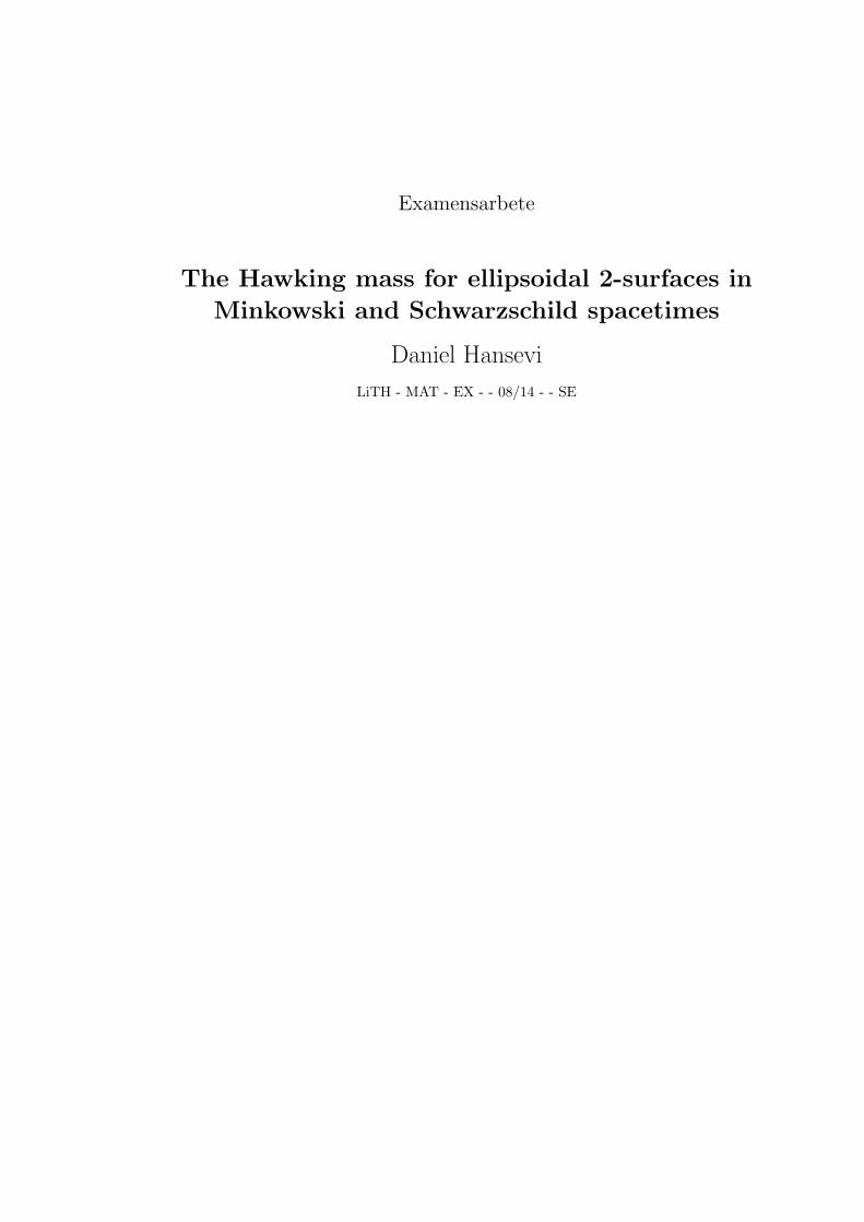
With a Lorentzian metric on M, all non-zero vectors in Tp can be dividedinto three classes. With our particular choice of signature, a vector va is saidto be

timelike if vava > 0,

null if vava = 0,

spacelike if vava < 0.

(2.21)

Thus, a Lorentzian metric defines a certain structure on each Tp, called a nullcone; the set of null vectors form what looks like a double cone if we suppressone spatial dimension, see figure 2.5.

future cone

past cone

p

spacelike vector

timelike vector

null vector

Figure 2.5: Null cone.

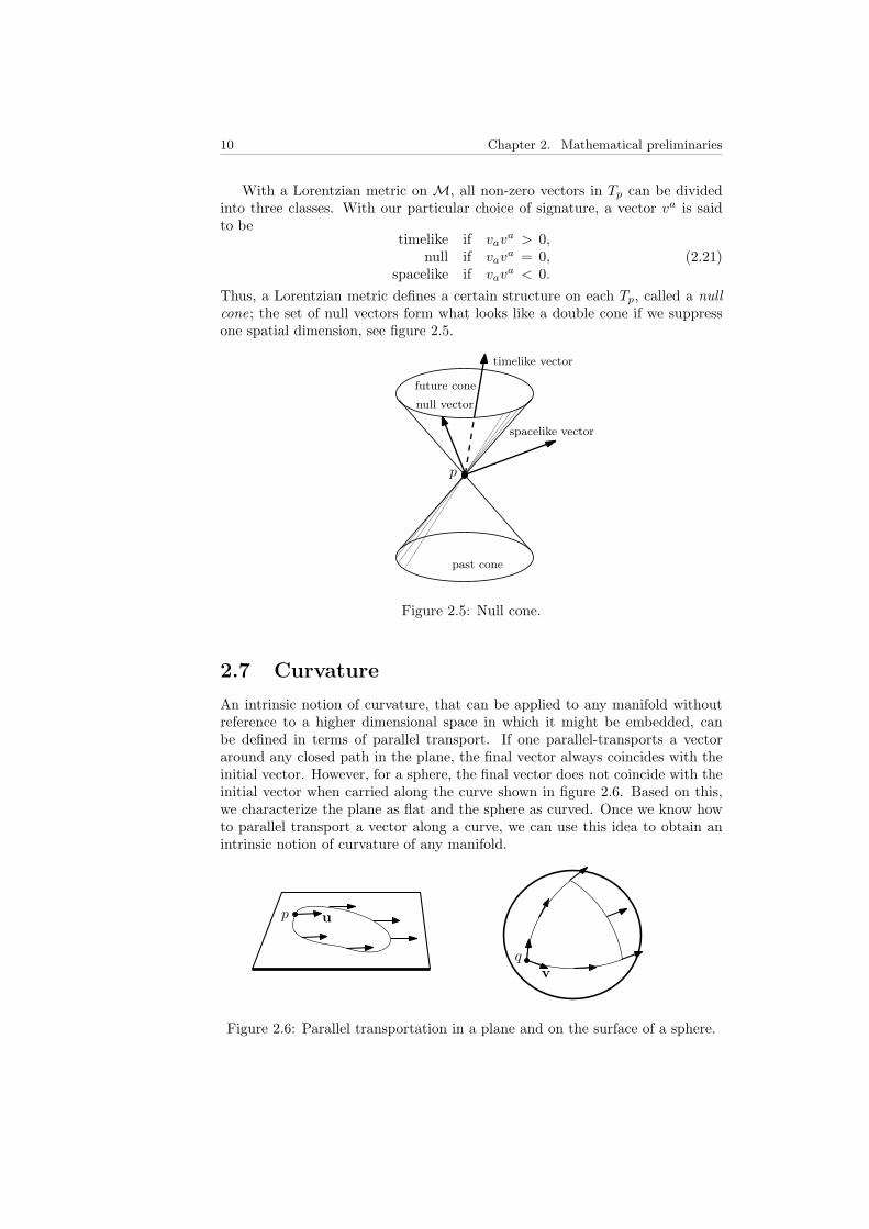
2.7 Curvature

An intrinsic notion of curvature, that can be applied to any manifold withoutreference to a higher dimensional space in which it might be embedded, canbe defined in terms of parallel transport. If one parallel-transports a vectoraround any closed path in the plane, the final vector always coincides with theinitial vector. However, for a sphere, the final vector does not coincide with theinitial vector when carried along the curve shown in figure 2.6. Based on this,we characterize the plane as flat and the sphere as curved. Once we know howto parallel transport a vector along a curve, we can use this idea to obtain anintrinsic notion of curvature of any manifold.

up

vq

Figure 2.6: Parallel transportation in a plane and on the surface of a sphere.

2.7. Curvature 11

Since the tangent spaces at two distinct points are different vector spaces itis not meaningful to say that a vector in the first tangent space equals a vectorin the latter. Thus, before we can define parallel transport, we must imposemore structure on the manifold.

Given a notion of a derivative operator, it is natural to define a vector to beparallel-transported if its derivative along the given curve is zero. The notionof curvature can be defined in terms of the failure of the final vector to coincidewith the initial vector when parallel transported around an infinitesimal closedcurve, which in turn corresponds to the lack of commutativety of derivatives.

2.7.1 Covariant derivative

A connection, or covariant derivative operator, ∇a on a smooth manifold Massigns to every vector field xa on M, a differential operator xa∇a that mapsan arbitrary vector field ya on M into a vector field xa∇ayb such that for allvector fields xa, ya, za and functions f on M:

(i) xa∇a(yb + zb) = xa∇ayb + xa∇azb (linear);

(ii) xa∇a(fyb) = (xa∇af)yb + f(xa∇ayb) (Leibniz’ rule);

(iii) xa∇af = x(f) (consistency with the notion of tangent vectors).

The vector field xa∇ayb is called the covariant derivative of ya with respect toxa, and the (1, 1)-tensor ∇ayb mapping xa to xa∇ayb the covariant derivativeof yb.

The definition of ∇a can be extended to apply to any tensor field on M bythe additional requirement that ∇a when acting on contracted products shouldsatisfy Leibniz’ rule.

2.7.2 Metric connection

A connection ∇a is not uniquely defined by the above conditions. In [14], how-ever, it is shown that if M is endowed with a metric gab, then there exists aunique connection ∇a with the properties that for all smooth functions f onM:

(i) ∇a gbc = 0 (compatible with metric);

(ii) ∇a∇bf − ∇b∇af = 0 (torsion-free).

This particular ∇a is called the metric connection, or the Levi-Civita4 connec-tion, on M, and has the properties that for all smooth vector fields ya on M:

∇ayb = ∂ayb + Γbacyc and ∇ayb = ∂ayb − Γcabyc, (2.22)

where ∂a is an ordinary derivative, and the Christoffel 5 symbol Γcab is given by

Γcab =12gcd(∂agbd + ∂bgad − ∂dgab

). (2.23)

Thus, in a given coordinate patch (U , φ) with coordinates xµ, the coordinatebasis components of ∇ayb are given by

∂yρ

∂xµ+

12

∑σ,ν

gρσ(∂gνσ∂xµ

+∂gµσ∂xν

− ∂gµν∂xσ

)yν . (2.24)

4Tullio Levi-Civita (1873-1941), Italian mathematician.5Elwin Bruno Christoffel (1829-1900), German mathematician.


2.7.3 Parallel transportation

Given a derivative operator ∇a we can define the notion of parallel transport.A smooth vector field ya is said to be parallelly transported around a curve withtangent vector xa if the equation

xa∇ayb = 0 (2.25)

is satisfied along the curve.The metric connection has the property that the inner product f = yaz

a

of any two smooth vector fields ya and za remains unchanged when parallellytransported along any curve with tangent vector xa, since

xa(f) = xa∇a(gbcybzc)= (xa∇agbc︸︷︷︸

=0

)ybzc + (xa∇ayb︸︷︷︸=0

)gbczc + (xa∇azc︸︷︷︸=0

)gbcyb. (2.26)

2.7.4 Curvature

Let ωa be any smooth 1-form field onM. The Riemann6 curvature tensor Rabcd

is the tensor field on M defined by,

(∇a∇b − ∇b∇a)ωc =: Rabcdωd, (2.27)

that is directly related to the failure of a vector to return to its initial valuewhen parallel transported around a small closed curve.7

For any smooth vector field ta on M, the corresponding expression is

(∇a∇b − ∇b∇a) tc = −Rabdctd. (2.28)

The Ricci 8 tensor is defined by contraction with respect to the second andfourth slot, Rac := Rabc

b, and the Ricci scalar curvature is defined by furthercontraction, R := Ra

a. The Ricci tensor and scalar curvature are used to definethe Einstein tensor,

Gab := Rab − 12Rgab, (2.29)

which is a fundamental tensor in general relativity.

2.7.5 Geodesics

Let xa be a smooth vector field onM. From the theory of ordinary differentialequations, we know that given a point p ∈M, there exists a unique curve thatpasses through p and has the property that for each point on the curve, thetangent vector of the curve coincides with the corresponding vector of xa. Sucha curve is called an integral curve.

Let xa be a smooth vector field such that xa∇axb = 0. Then the integralcurves of xa are called geodesics.

6Georg Friedrich Bernhard Riemann (1826-1866), German mathematician.7Some authors reverse the sign of the left-hand side in the definition.8Gregorio Ricci-Curbastro (1853-1925), Italian mathematician.

2.7. Curvature 13

Geodesics are curves that are ‘as straight as possible’, and it can be shown[14] that there is precisely one geodesic through a given point p ∈M in a givendirection xa ∈ Tp.

Let λs(t) be a one-parameter family of geodesics and consider the two-dimensional surface, with coordinates (t, s), spanned by λs(t). The vector fieldxa = (∂/∂t)a is tangent to the family of geodesics, thus

xa∇axb = 0, (2.30)

and the vector field ya = (∂/∂s)a represents the deviation vector, which is thedisplacement from the geodesic λs to an ‘infinitesimally’ nearby geodesic λs′ ,see figure 2.7.

ya

xaxa

λs

λs′

Figure 2.7: Deviation vector ya between two nearby geodesics λs and λs′ .

Let f be any smooth function on M. Since

(xa∇ayb − ya∇axb)∇bf = xa∇a(yb∇bf) − ya∇a(xb∇bf)= x(y(f)) − y(x(f))

=∂2f

∂t∂s− ∂2f

∂s∂t= 0, (2.31)

it follows thatxa∇ayb = ya∇axb. (2.32)

The relative acceleration za, in the direction of ya, of a nearby geodesic whenmoving along the direction of xa, is given by

za = xc∇c(xb∇bya)(2.32)

= xc∇c(yb∇bxa)= (xc∇cyb)∇bxa + yb(xc∇c∇bxa)

(2.28)= (yc∇cxb)∇bxa + yb(xc∇b∇cxa) − Rcbd

aybxcxd

= yc∇c(xb∇bxa) − Rcbdaybxcxd

(2.25)= −Rcbdaybxcxd. (2.33)

Thus, the geodesic deviation, that is, the acceleration of geodesics toward oraway from each other, which is a characterization of the curvature of M, isdetermined by the Riemann curvature tensor. M is flat if and only if Rabcd = 0.


2.8 Tetrad formalism

The tetrad formalism (or frame formalism) is a useful technique for derivinguseful and compact equations in many applications of general relativity. Theidea is to use a so called tetrad basis of four linearly independent vector fields,project the relevant quantities onto the basis, and consider the equations satis-fied by them.

Let eia, i = 1, 2, 3, 4, be smooth vector fields that are linearly independentat each point in spacetime (M, gab). Then the Ricci rotation coefficients aredefined by

γkij := ekcej

a∇aeic. (2.34)

It is shown in [2] that

γijk =12

(λijk + λkij − λjki), where λijk = (∂beja − ∂aejb)eiaekb, (2.35)

which is an efficient way of calculating the Ricci rotation coefficients, since thereis no need to calculate any covariant derivatives.

2.9 Newman-Penrose formalism

The tetrad formalism with the choice of a particular type of null basis, intro-duced by Ezra Newman and Roger Penrose [9] in 1962, is usually called theNewman-Penrose formalism. The basis la, na, ma, ma consists of null vec-tors, where la and na are real, ma and ma are complex conjugates, satisfying

la la = na n

a = mama = ma m

a = 0 (null);lam

a = la ma = nam

a = na ma = 0 (orthogonal);

la na = −ma m

a = 1 (normalized).(2.36)

2.10 Spin coefficients

In the Newman-Penrose formalism, the Ricci rotation coefficients are called spincoefficients, and are given in figure 2.8.

κ = γ311 κ′ = −ν = γ422 2α = γ214 + γ344

ρ = γ314 ρ′ = −µ = γ423 2β = γ213 + γ343

σ = γ313 σ′ = −λ = γ424 2γ = γ212 + γ342

τ = γ312 τ ′ = −π = γ421 2ε = γ211 + γ341

Figure 2.8: Spin coefficients.

The spin coefficients ρ and ρ′ are of particular interest to us, since they are usedin the definition of the Hawking mass.

Chapter 3

General relativity

General relativity is the modern geometric theory of space, time and gravitationpublished by Albert Einstein [4] in 1916. In the theory, space and time are uni-fied into spacetime (M, gab), which is represented by a smooth four-dimensionalHausdorff manifoldM endowed with a Lorentzian metric gab and a metric con-nection ∇a. The presence of matter ‘warps’ spacetime according to the Einsteinfield equation,

Gab := Rab − 12Rgab = 8π Tab, (3.1)

where Gab is the Einstein tensor that describes the curvature of M and Tabis the stress-energy-momentum tensor describing the distribution of matter.1

Free particles travel along timelike geodesics and light rays travel along nullgeodesics. Thus gravity is a manifestation of the curvature of spacetime.

Space acts on matter, telling it how to move. In turn, matter reactsback on space, telling it how to curve.2

3.1 Solutions to the Einstein field equation

The Einstein field equation might look simple when written with tensors. How-ever, it constitutes a system of coupled, non-linear partial differential equations.

3.1.1 Minkowski spacetime

The spacetime of special relativity – Minkowski3 spacetime – is a solution tothe vacuum field equation Gab = 0. It is the flat4 spacetime (M, ηab) given bythe constant metric

(ηab) =

1 0 0 00 −1 0 00 0 −1 00 0 0 −1

. (3.2)

1Some authors use a different sign in the definition of the Ricci tensor resulting in aminus sign in front of the right-hand side. Furthermore, we use ‘geometrized units’ where thegravitational constant G, and the speed of light c, are set equal to one.

2Brief explanation of general relativity by the ‘student’ portrayed in chapter one of [8].3Hermann Minkowski (1864-1909), Russian-born German mathematician.4Rabc

d = 0.

Hansevi, 2008. 15

16 Chapter 3. General relativity

In the coordinate system implied by ηab, all geodesics appear straight, that is,they take the form, xa(t) = ya + zat.

3.1.2 Schwarzschild spacetime

One of the solutions of the vacuum field equation was discovered by KarlSchwarzschild5 in 1916, just a couple of months after Einstein published hisfield equation. The Schwarzschild solution is the unique solution that describesthe curved spacetime exterior to a static spherically symmetric mass, such as a(non-rotating) star, planet, or black hole, and it remains one of the most impor-tant exact solutions. Schwarzschild spacetime is the curved spacetime (M, gab)given, in Schwarzschild coordinates, by the metric

(gab) =

1 − 2M

r 0 0 0

0 −(

1 − 2Mr

)−1

0 00 0 − r2 00 0 0 − r2 sin2 θ

. (3.3)

In these coordinates, the metric becomes singular at the surface r = 2M , whichis called the event horizon. Events inside (or on) this surface cannot affect anoutside observer; nothing can escape to the outside, not even light.

5Karl Schwarzschild (1873-1916), German physicist.

Chapter 4

Mass in general relativity

The stress-energy-momentum tensor, Tab, is the tensor that describes the den-sity and flux of energy and momentum in spacetime. It represents the energydue to matter and electromagnetic fields. Mass is the source of gravity, andenergy is associated with mass,1 therefore Tab is in the right-hand side of theEinstein field equation ‘telling spacetime how to curve.’

4.1 Gravitational energy/mass

Imagine a system of two massive bodies at rest relative to each other. If theyare far apart, then there will be a gravitational potential energy contributionthat makes the total energy of the system greater than if they are close to eachother. There is a difference in total energy, despite that integrating the energydensities, Tab, yields the same result in both scenarios. That energy differenceis the energy attributed to the gravitational field. Since the gravitational fieldhas energy, and therefore mass, it is a source of gravity, hence it is coupled toitself. Mathematically, this is possible because the field equation is non-linear.

4.1.1 Non-locality of mass

The contribution of gravitational mass should be included in a description fortotal mass in a spacelike volume of spacetime. The stress-energy-momentumtensor Tab is given as a pointwise density and can be integrated over the volume.Can the gravitational mass be given as a point density that we can integrate?The answer is no. At any point in spacetime, one can always find a localcoordinate system (Riemann-normal coordinates) in which all Christoffel symbolcomponents vanish, which mean that there is no local gravitational field, henceno local gravitational mass [8, 14]. In such a coordinate system, an observerin ‘free fall’ moves along a straight line, and does not ‘feel’ any gravitationalforces.

1According to E = mc2; Einstein’s famous equation [3].

Hansevi, 2008. 17

18 Chapter 4. Mass in general relativity

4.2 Total mass of an isolated system

Despite the fact that the gravitational mass cannot be given as a pointwisedensity, there exist meaningful notions of the total mass of an ‘isolated system’.

4.2.1 Asymptotically flat spacetimes

Say that we want to study the system of the two massive bodies (of section4.1). Even though no physical system can be truly isolated from the rest of theuniverse, we can simplify our model by pretending that the system is isolated,ignoring the influence of distant matter. The spacetime of our simplified modelwill have vanishing curvature at large distances from the two bodies, and wesay that it is asymptotically flat. A precise and useful, but rather technical,definition of an asymptotically flat spacetime is given in [14].

4.2.2 ADM and Bondi-Sachs mass

In asymptotically flat spacetimes, the total mass can be determined by theasymptotic form of the metric. The ADM2 mass is the total mass measuredat spacelike infinity, whereas the Bondi-Sachs3 mass is measured at future nullinfinity [14].

4.3 Quasi-local mass

A meaningful definition of mass at a quasi-local level, that is, for the mass withina compact spacelike 2-surface, should have certain properties. For example, thequasi-local mass should be uniquely defined for all domains. Furthermore, itshould be strictly positive (except in the flat case, where it should be equal tozero). Its limits at spacelike infinity and future null infinity should be the ADMmass and Bondi-Sachs mass, respectively. It should be monotone, that is, themass for a domain should be greater or equal to the mass for a domain that iscontained in the first.

One can ask if it is possible to find a satisfying definition of mass at a quasi-local level. Several attempts have been made, for example, the Dougan-Masonmass, the Komar mass, the Penrose mass, and the Hawking mass. However,they fail to agree on the mass for a spacelike cross section of the event horizonof a Kerr4 black hole [1]. There is still no generally accepted definition.

To reach an appropriate definition for quasi-local mass would certainly be ofgreat value. It could give a more detailed characterization of the gravitationalfield around massive bodies, and it should be helpful for controlling errors innumerical calculations [13].

2R. Arnowitt, S. Deser and C. Misner.3H. Bondi and R. K. Sachs.4A solution to the Einstein field equation found in 1963 by Roy Kerr. It describes spacetime

outside a rotating black hole.

Chapter 5

The Hawking mass

One of many suggestions that have been made for a definition of quasi-localmass originates from a paper about gravitational radiation written by StephenHawking [5] in 1968 .

The Hawking mass has been shown to have various desirable properties, forexample, the limits at spacelike infinity and future null infinity are the ADMmass and the Bondi-Sachs mass, respectively [13]. Its advantage is its simplicity,calculability and monotonicity for special families of 2-surfaces. In Minkowskispacetime, the Hawking mass vanish for 2-spheres. However, it can give negativeresults for general 2-surfaces, for example for non-convex 2-surfaces.

5.1 Definition

Let la and na be, respectively, the outgoing and the ingoing null vectors orthog-onal to a spacelike 2-sphere S and let ma and ma be tangent vectors to S. Thenthe Hawking mass is defined by

mH(S) :=

√Area(S)

16π

(1 +

12π

∮Sρρ′dS

). (5.1)

5.2 Interpretation

Consider a one-parameter family of null geodesics, that is light rays, that inter-sects a circle in a 2-plane. Following the geodesics in the future direction, theoptical scalars, θ and σ, introduced by Rainer Sachs [12] in 1961, can be definedas

θ = Re ρ and σ = Im ρ, (5.2)

and interpreted as the expansion and rotation, respectively, of the circle [2].Both la and na are orthogonal to the surface, thus both ρ and ρ′ are real [10].Hence ρ and ρ′ measure the expansion of outgoing and ingoing null geodesics,respectively, and the Hawking mass can be viewed as a measure of the bending ofoutgoing and ingoing light rays orthogonal to the surface of a spacelike 2-sphere.

Hansevi, 2008. 19

20 Chapter 5. The Hawking mass

5.3 Method for calculating spin coefficients

In this section, a method for calculating the spin coefficients used in the expres-sion for the Hawking mass is provided.

• In order to calculate the required spin coefficients (section 2.10), introducea coordinate system such that for a given r, and t held fixed, 0 ≤ θ < πand 0 ≤ ϕ < 2π trace out the surface S.

• In the new coordinates, every vector with the first two components van-ished lies in the tangent plane of S, as ma is required to do. The other twovectors, la and na, are parallel to the outgoing and ingoing null directions,respectively, thus it is convenient to set up a null tetrad (la, na, ma, ma),by making the ansatz la = ( A B C 0 ),

na = ( A −B −C 0 ),ma = ( 0 0 X iY ).

(5.3)

By imposing the conditions (2.36) to (5.3), A, B, C, X and Y can bedetermined by solving the obtained equations in three steps.

1. Solve the systemmam

a = 0 (null vector)ma m

a = −1 (normalization) , (5.4)

and pick one solution X,Y .2. Solve the system

la la = 0 (null vector)

la na = 1 (normalization) , (5.5)

and pick the solution A,B, where A > 0 (and B > 0 if possible).The solution will possibly be dependent of C.

3. Determine C (and A and B if they depend on C) by solving

lama = 0 (orthogonality) . (5.6)

The result of the procedure above is a null tetrad (la, na, ma, ma) satis-fying the conditions (2.36).

• Calculate the spin coefficients with the use of the null tetrad by firstcalculating the required λijk given by (2.35),

λ314 = (∂b la − ∂a lb) ma mb

λ431 = (∂bma − ∂amb) ma lb

λ143 = (∂b ma − ∂a mb) lamb

λ423 = (∂b na − ∂a nb) mamb

λ342 = (∂b ma − ∂a mb) ma nb

λ234 = (∂bma − ∂amb) na mb

, (5.7)

then the spin coefficients follow easily as,

ρ = γ314 = (λ314 + λ431 − λ143)/2ρ′ = γ423 = (λ423 + λ342 − λ234)/2 . (5.8)

5.4. Hawking mass for a 2-sphere 21

5.4 Hawking mass for a 2-sphere

In the following subsections, we demonstrate the method of section 5.3 by cal-culating the Hawking mass for a 2-sphere.

5.4.1 In Minkowski spacetime

Using coordinates (t, r, θ, ϕ), where the spatial part (r, θ, ϕ) is written in spher-ical polar coordinates, the Minkowski metric (3.2) can be written as,

(gab) =

1 0 0 00 −1 0 00 0 −r2 00 0 0 −r2 sin2 θ

. (5.9)

By solving the equations (5.4), (5.5) and (5.6) in three steps, we obtain the nulltetrad (la, na, ma, ma), given by

la =√

22

(1 1 0 0

),

na =√

22

(1 −1 0 0

), (5.10)

ma =√

22

(0 0

1r

−ir sin θ

),

and then it follows easily from (5.7) and (5.8) that

ρρ′ = − 12r2

. (5.11)

The area of the 2-sphere is the familiar

Area(Sr) =

2π∫0

π∫0

r2 sin θ dθ dϕ = 4πr2, (5.12)

and the integral of the spin coefficients

∮Sr

ρρ′dS =

2π∫0

π∫0

−12

sin θ dθ dϕ = −2π. (5.13)

Finally, we can confirm the well-known result that the Hawking mass vanish forall 2-spheres in Minkowski spacetime, since

mH(Sr) =

√4πr2

16π

(1 +

12π

(−2π))

=r

2(1 − 1

)= 0. (5.14)

5.4.2 In Schwarzschild spacetime

We repeat the calculations of the previous section, but this time for a cen-tered 2-sphere in Schwarzschild spacetime. The coordinates (t, r, θ, ϕ) of the

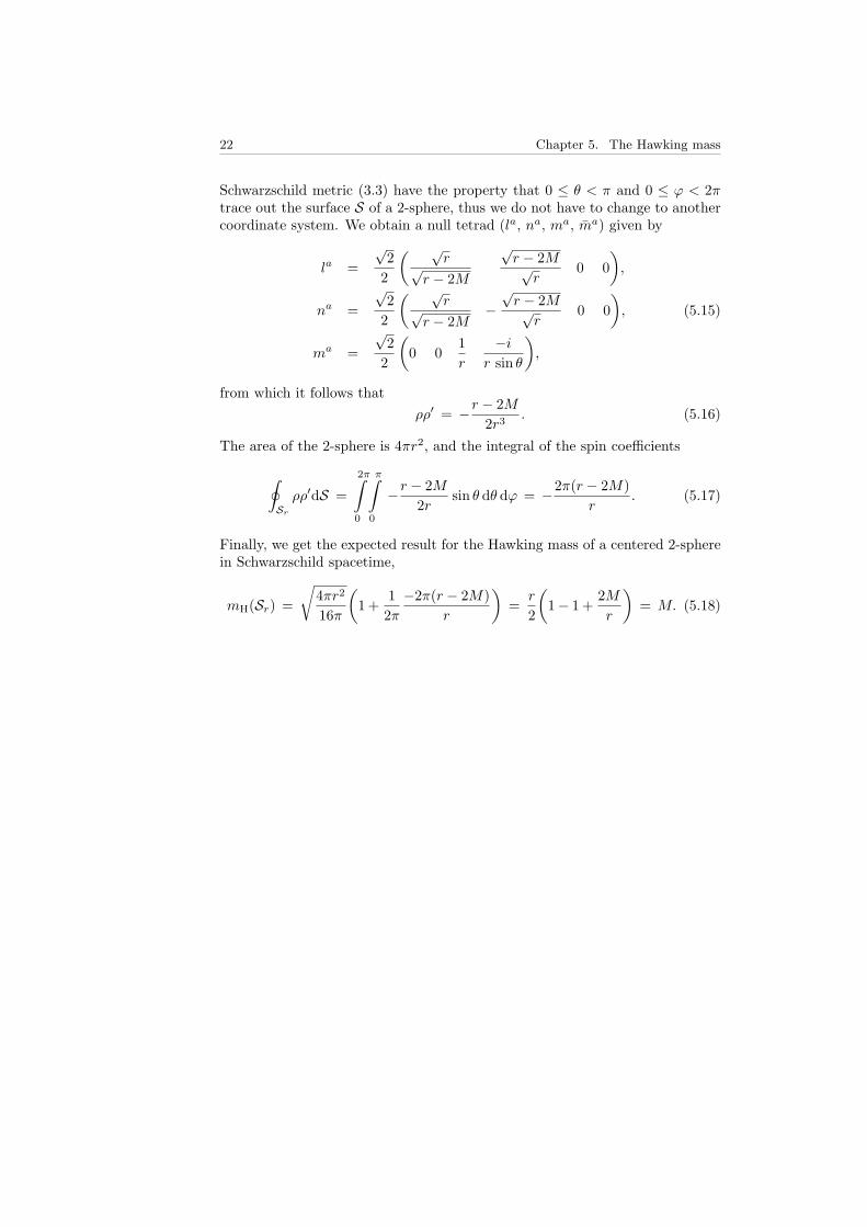
22 Chapter 5. The Hawking mass

Schwarzschild metric (3.3) have the property that 0 ≤ θ < π and 0 ≤ ϕ < 2πtrace out the surface S of a 2-sphere, thus we do not have to change to anothercoordinate system. We obtain a null tetrad (la, na, ma, ma) given by

la =√

22

( √r√

r − 2M

√r − 2M√

r0 0

),

na =√

22

( √r√

r − 2M−√r − 2M√

r0 0

), (5.15)

ma =√

22

(0 0

1r

−ir sin θ

),

from which it follows thatρρ′ = −r − 2M

2r3. (5.16)

The area of the 2-sphere is 4πr2, and the integral of the spin coefficients

∮Sr

ρρ′dS =

2π∫0

π∫0

−r − 2M2r

sin θ dθ dϕ = −2π(r − 2M)r

. (5.17)

Finally, we get the expected result for the Hawking mass of a centered 2-spherein Schwarzschild spacetime,

mH(Sr) =

√4πr2

16π

(1 +

12π−2π(r − 2M)

r

)=

r

2

(1− 1 +

2Mr

)= M. (5.18)

Chapter 6

Results

In this chapter, we calculate the Hawking mass, with the aid of Maple1, forellipsoidal 2-surfaces in both Minkowski and Schwarzschild spacetimes. Thecalculations for Minkowski are performed symbolically, and the results are pre-sented as a theorem and two corollaries.

In Schwarzschild spacetime, the Hawking mass are calculated numericallyfor approximately ellipsoidal 2-surfaces, and the results are therefore presentedwith diagrams.

First, we prove a lemma that will be useful in section 6.1.

Lemma 6.1. Assume that ξ > 1. Then

arccosh ξ√ξ2 − 1

= 1− ξ − 13

+2(ξ − 1)2

15+O((ξ − 1)5/2

).

Proof. Consider the equivalence,

ξ =√x2 + 1, x > 0 ⇐⇒ x =

√ξ2 − 1, ξ > 1, (6.1)

and the following Maclaurin expansions [11],√x2 + 1 = 1 + x2/2− x4/8 +O(x6), (6.2)

ln(y + 1) = y − y2/2 + y3/3− y4/4 + y5/5 +O(y6). (6.3)

Perform a change of variable,


(def.)=

ln(ξ +√ξ2 − 1)√

ξ2 − 1(6.1)=

ln(√x2 + 1 + x

)x

, (6.4)

and apply the Maclaurin expansions to the numerator,

ln(√

x2 + 1 + x) (6.2)

= ln(1 + x+

x2

2− x4

8+O(x6)

)(6.3)= x+

x2

2− x4

8+O(x6)−

(x+ x2

2 − x4

8 +O(x6))2

21Mathematics software package from Waterloo Maple Inc.

Hansevi, 2008. 23

24 Chapter 6. Results

+

(x+ x2

2 +O(x4))3

3−(x+ x2

2 +O(x4))4

4

+

(x+O(x2)

)55

+O(x6)

= x− x3

6+

3x5

40+O(x6). (6.5)

Divide through by x, and change back to ξ,


= 1− ξ2 − 16

+3(ξ2 − 1)2

40+O((ξ2 − 1)5/2

). (6.6)

Since ξ > 1, the ordo-term is actually

O((ξ2 − 1)5/2)

= O((ξ + 1)5/2(ξ − 1)5/2)

= O((ξ − 1)5/2). (6.7)

Thus, let

f(ξ) = 1− ξ2 − 16

+3(ξ2 − 1)2

40, (6.8)

and calculate the second degree Taylor expansion of f about ξ = 1 . Fromf(1) = 1, f ′(1) = −1/3, and f ′′(1) = 4/15 it follows that


= 1− ξ − 13

+2(ξ − 1)2

15+O((ξ − 1)5/2

). (6.9)

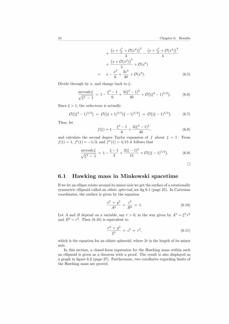
6.1 Hawking mass in Minkowski spacetime

If we let an ellipse rotate around its minor axis we get the surface of a rotationallysymmetric ellipsoid called an oblate spheriod, see fig 6.1 (page 25). In Cartesiancoordinates, the surface is given by the equation

x2 + y2

A2+

z2

B2= 1. (6.10)

Let A and B depend on a variable, say r > 0, in the way given by A2 = ξ2 r2

and B2 = r2. Then (6.10) is equivalent to

x2 + y2

ξ2+ z2 = r2, (6.11)

which is the equation for an oblate spheroid, where 2r is the length of its minoraxis.

In this section, a closed-form expression for the Hawking mass within suchan ellipsoid is given as a theorem with a proof. The result is also displayed asa graph in figure 6.2 (page 27). Furthermore, two corollaries regarding limits ofthe Hawking mass are proved.

6.1. Hawking mass in Minkowski spacetime 25

Figure 6.1: Oblate spheroid.

6.1.1 Closed-form expression of the Hawking mass

Theorem 6.1. Let (M, ηab) be Minkowski spacetime. For ξ > 1, let Sr be thespacelike oblate 2-spheroids, in M, given by

Sr =

(x2 + y2)/ξ2 + z2 = r2 : r > 0.

Then the Hawking mass within Sr is given by

mH

(Sr) =−√2 r16√ξ

√ξ +


(2 ξ2 − 5

3ξ +


).

Proof. Use the method provided in section 5.3. Start by introducing a coordi-nate system such that for a given r, and t held fixed, θ and ϕ trace out theellipsoidal 2-surface Sr. This is accomplished by using the parametrized formof Sr, x = ξ r sin θ cosϕ

y = ξ r sin θ sinϕz = r cos θ

,

0 < r0 ≤ θ < π0 ≤ ϕ < 2π

, (6.12)

as new variables (t, r, θ, φ).Using the tensor transformation law (2.19) yields the Minkowski metric (3.2)

in the new coordinates,

(gab) =

1 0 0 00 −(cos2 θ + ξ2 sin2 θ) −(ξ2 − 1)r cos θ sin θ 00 −(ξ2 − 1)r cos θ sin θ −r2(ξ2 cos2 θ + sin2 θ) 00 0 0 −ξ2r2 sin2 θ

.

(6.13)Ansatz (5.3).

• Solve equations (5.4), and pick a solution, sayX = 1 / (

√2 r√ξ2 cos2 θ + sin2 θ)

Y = 1 / (√

2 ξ r sin θ). (6.14)

• Solve equations (5.5), and pick the solution given by A = 1/√

2 and

B =

√cos2 θ + ξ2 sin2 θ − 2ξ2 r2 C2 − √2(ξ2 − 1) r cos θ sin θ C√

2(cos2 θ + ξ2 sin2 θ).

(6.15)


• Solve equation (5.6). The solution is given by

C = −√

2(ξ2 − 1) cos θ sin θ

2 ξ r√ξ2 cos2 θ + sin2 θ

. (6.16)

The result of this procedure is the null tetrad (la, na, ma, ma), given by

la =√

22

(1

√ξ2 cos2 θ + sin2 θ

ξ− (ξ2 − 1) cos θ sin θ

ξ r√ξ2 cos2 θ + sin2 θ

0),

na =√

22

(1 −

√ξ2 cos2 θ + sin2 θ

ξ

(ξ2 − 1) cos θ sin θ

ξ r√ξ2 cos2 θ + sin2 θ

0),

ma =√

22

(0 0

1

r√ξ2 cos2 θ + sin2 θ

i

ξ r sin θ

),

ma =√

22

(0 0

1

r√ξ2 cos2 θ + sin2 θ

− i

ξ r sin θ

). (6.17)

Calculate the spin coefficients with the use of the null tetrad by first calcu-lating the required λijk given by (5.7),

λ314 = (∂b la − ∂a lb)ma mb = 0,

λ431 = (∂bma − ∂amb)ma lb = − ξ2 (1 + cos2 θ) + sin2 θ

2√

2 ξ r (ξ2 cos2 θ + sin2 θ)3/2,

λ143 = (∂b ma − ∂a mb)lamb =ξ2 (1 + cos2 θ) + sin2 θ

2√

2 ξ r (ξ2 cos2 θ + sin2 θ)3/2,

λ423 = (∂b na − ∂a nb)mamb = 0,

λ342 = (∂b ma − ∂a mb)ma nb =ξ2 (1 + cos2 θ) + sin2 θ

2√

2 ξ r (ξ2 cos2 θ + sin2 θ)3/2,

λ234 = (∂bma − ∂amb)na mb = − ξ2 (1 + cos2 θ) + sin2 θ

2√

2 ξ r (ξ2 cos2 θ + sin2 θ)3/2,

(6.18)

then the spin coefficients (5.8) follow easily as,

ρ = γ314 = − ξ2(1 + cos2 θ) + sin2 θ

2√

2 ξ r(ξ2 cos2 θ + sin2 θ

)3/2 ,ρ ′ = γ423 =

ξ2(1 + cos2 θ) + sin2 θ

2√

2 ξ r(ξ2 cos2 θ + sin2 θ

)3/2 . (6.19)

The surface area of Sr is part of the expression for the Hawking mass. Fromthe surface element dS =

√gθθ gϕϕ − (gθϕ)2 dθ dϕ it follows that

Area(Sr) =

2π∫0

π∫0

ξ r2 sin θ√ξ2 cos2 θ + sin2 θ dθ dϕ

=2π ξ r2

(ξ√ξ2 − 1 + ln(

√ξ2 − 1 + ξ)

)√ξ2 − 1

6.1. Hawking mass in Minkowski spacetime 27

= 2π ξ r2(ξ +


), (6.20)

Integration over Sr yields

2π∫0

π∫0

ρρ ′ dS =

2π∫0

π∫0

sin θ(ξ2(1 + cos2 θ) + sin2 θ

)2ξ(ξ2 cos2 θ + sin2 θ

)5/2 dθ dϕ

= −π6

(2 ξ3 + 7ξ)√ξ2 − 1 + 3 arcsinh (

√ξ2 − 1)

ξ√ξ2 − 1

= −π6

(2 ξ2 + 7 +

3ξ


). (6.21)

Finally, from (6.20) and (6.21), the Hawking mass in Sr follows as

mH(Sr) =

√Area(Sr)

16π

(1 +

12π

2π∫0

π∫0

ρρ ′ dS)

=−√2 r16√ξ

√ξ +


(2 ξ2 − 5

3ξ +


). (6.22)

As can be seen in figure 6.2, the Hawking mass becomes negative in Minkowski,even for a convex 2-surface.

1 2 3 40−3

−2

−1

0

1

Figure 6.2: mH(S1) plotted against parameter ξ.

6.1.2 Limit when approaching a metric sphere

Corollary 6.1. Let (M, ηab) be Minkowski spacetime. Given an r > 0, theHawking mass vanishes in the limit when ξ → 1+, that is, when Sr tends to a2-sphere.

Proof. It follows from lemma 6.1 that


= 1− ξ − 13

+2(ξ − 1)2

15+O((ξ − 1)5/2

)= 1 +O(ξ − 1), (6.23)


and furthermore that

2 ξ2 − 53

ξ +arccosh ξ√ξ2 − 1

=2 ξ3

3− 5 ξ

3+ 1 +O(ξ − 1)

=2 ξ(ξ + 1)− 3

3(ξ − 1

)+O(ξ − 1)

= O(ξ − 1). (6.24)

Thus, it follows from (6.23), (6.24) and theorem 6.1 that

mH(Sr) =−√2 r16√ξ

√ξ +


(2 ξ2 − 5

3ξ +


)=

r√ξ

√1 + ξ +O(ξ − 1)O(ξ − 1)→ 0 as ξ → 1+. (6.25)

6.1.3 Limit along a foliation

Corollary 6.2. Let (M, ηab) be Minkowski spacetime. For ω > 0, let Lrr>0

be foliations of a spacelike 3-surface Ω ⊂M. Suppose that the leaves are givenby

Lr =

(x2 + y2)/(1 + ω/r)2 + z2 = r2 : r > 0.

Then the Hawking mass vanishes in the limit along all foliations Lrr>0.

Proof. Observe thatLr = Sr

∣∣∣ξ=1+ω/r

, (6.26)

and let ξ = 1 + ω/r in lemma 6.1. Then ξ → 1+ as r →∞, and it follows that

1 + ω/r +arccosh (1 + ω/r)√

(1 + ω/r)2 − 1= 1 +

ω

r+ 1− ω

3r+

2ω2

15r2+O

( 1r5/2

)= 2 +

2ω3r

+2ω2

15r2+O

( 1r5/2

)= 2 +O

(1r

), (6.27)

and furthermore that

2(1 + ω/r)2 − 53

(1 + ω/r) +arccosh (1 + ω/r)√

(1 + ω/r)2 − 1=

32ω2

15r2+

2ω3

3r3+O

( 1r5/2

)= O

( 1r2

). (6.28)

From (6.27) and theorem 6.1, it follows that

mH(Lr) =−√2 r

16√

1 + ωr

√2 +O

(1r

)O( 1r2

)= O

(1r

)→ 0 as r →∞. (6.29)

6.2. Hawking mass in Schwarzschild spacetime 29

6.2 Hawking mass in Schwarzschild spacetime

In this section we will study the Hawking mass in the curved Schwarzschildspacetime. A consequence of the spacetime being curved is that the requiredcalculations tend to be more complicated. Considering this, we will calculate theHawking mass for an approximately ellipsoidal 2-surface, exterior to the eventhorizon (r > 2M), that has a simple expression in spherical polar coordinates.

For small ε > 0, let the curve given by

r =√

1 + ε sin2 θ, (6.30)

rotate around the axis θ = 0. See figure 6.3. The surface of revolution, S, isapproximately ellipsoidal. For ε = 0, it is a perfect sphere.

θ = 0

rθ

Figure 6.3: A curve given by r =√

1 + ε sin2 θ.

Let us introduce a coordinate system such that for a given r, and t heldfixed, θ and ϕ trace out the spacelike 2-surface Sr. This is accomplished by thefollowing change of variables,

r 7→ r√

1 + ε sin2 θ, r > 2M. (6.31)

In the new coordinates, the Schwarzschild metric (3.3) is given by

(gab) =

βrα 0 0 00 − rα3

β − εr2α cos θ sin θβ 0

0 − εr2α cos θ sin θβ − r2(α3β+ε2r cos2 θ sin2 θ)

αβ 00 0 0 −r2α2 sin2 θ

,

(6.32)where

α =√

1 + ε sin2 θ > 1 and β = r√

1 + ε sin2 θ − 2M > 0. (6.33)

By making the ansatz (5.3), solving equations (5.4), (5.5) and (5.6), weobtain a null tetrad (la, na, ma, ma) given by,

la =√

22

(√rα√β

√α3β + ε2r cos2 θ sin2 θ√

rα3

2C√2

0),


na =√

22

(√rα√β

−√α3β + ε2r cos2 θ sin2 θ√

rα3− 2C√

20), (6.34)

ma =√

22

(0 0

√αβ

r√α3β + ε2r cos2 θ sin2 θ

− i

rα sin θ

),

where

C = −√

22

ε cos θ sin θ√rα√α3β + ε2 r cos2 θ sin2 θ

. (6.35)

We calculate the spin coefficients ρ and ρ′. Unfortunately, their expressionsin Schwarzschild spacetime are very long, so we omit writing them out.

The surface element of Sr is given by

dS =√gθθ gϕϕ − (gθϕ)2 dθ dϕ

= r2α2 sin θ

√ε2 r cos2 θ sin2 θ

αβ+ 1 dθ dϕ, (6.36)

and the surface area by

Area(Sr) =

2π∫0

π∫0

dS. (6.37)

Since the expression of the Hawking mass for Sr,

mH(Sr) =

√Area(Sr)

16π

(1 +

12π

2π∫0

π∫0

ρρ′ dS), (6.38)

is rather complicated, we will rely on methods like Taylor expansion and nu-merical integration for further investigations.

6.2.1 Limit along a foliation

Analogously to corollary 6.2, let Lrr>2M be foliations of a spacelike 3-surfaceΩ ⊂ M (now in Schwarzschild spacetime). Suppose that the leaves, Lr, aregiven by substituting

ε =ω

r, r > 2M, (6.39)

into Sr. It is easy to see that Lr becomes more spherical the larger r gets.In this section, we will show that the limit of the Hawking mass of Lr is M

along all foliations Lrr>2M , that is,

limr→∞mH(Lr) = M. (6.40)

Since both dS and ρρ′dS are independent of ϕ, we make the substitution(6.39), and let

I1(ε) = ε2Area(Lω/ε) =: 2π∫ π

0

Φ(ε, θ) dθ (6.41)

6.2. Hawking mass in Schwarzschild spacetime 31

andI2(ε) = 2π

∫ π

0

ρρ′ dθ =: 2π∫ π

0

Ψ(ε, θ) dθ. (6.42)

Under the reasonable assumption that Φ(ε, θ), Φ′ε(ε, θ), Ψ(ε, θ), Ψ′ε(ε, θ) andΨ′′εε(ε, θ) are continuous in some neighbourhood |ε| < 1, it follows by Maclaurinexpansion that

I1(ε) = 2π∫ π

0

Φ(0, θ) dθ + O(ε) = 4πω2 + O(ε), |ε| < 1, (6.43)

and

I2(ε) = 2π∫ π

0

Ψ(0, θ) dθ + 2π∫ π

0

Ψ′ε(0, θ) dθ ε + O(ε2)

= −2π +4πMω

ε + O(ε2), |ε| < 1. (6.44)

Thus

Area(Lr) = I1(ε)/ε2 =4πω2

ε2+ O

(1ε

)= 4πr2 + O(r), r > |ω|, (6.45)

and2π∫ π

0

ρρ′ dS = −2π +4πMr

+ O( 1r2

), r > |ω|. (6.46)

By using the results (6.45) and (6.46), it follows that

mH(Lr) =

√4πr2 +O(r)

16π

(1 +

12π

[− 2π +

4πMr

+ O( 1r2

)])=

r

2

√1 +O

(1r

)(2Mr

+ O( 1r2

))=

√1 +O

(1r

)(M + O

(1r

))→ M as r → ∞.

(6.47)

6.2.2 Numerical evaluations

We evaluate the Hawking mass numerically with an adaptive Gaussian2 quadra-ture method.

In numerical quadrature, an integral

I(f) =∫ b

a

f(x)dx, (6.48)

is approximated by an n-point quadrature rule that has the form

Qn(f) =n∑i=1

wif(xi), (6.49)

where a ≤ x1 < x2 < · · · < xn ≤ b. The points xi are called nodes, and themultipliers wi are called weights.

2Carl Friedrich Gauss (1777-1855), German mathematician known as ‘princeps mathemati-corum’ (‘prince of mathematicians’).


In Gaussian quadrature, both the nodes and the weights are optimally cho-sen, hence Gaussian quadrature has the highest possible accuracy for the numberof nodes used. Furthermore, it is stable and Qn(f)→ I(f) as n→∞ [6].

In adaptive quadrature, the interval of integration is selectively refined toreflect the behavior of the particular integrand.

We set M = 1, and let Maple calculate the Hawking mass numerically forsome values of ε. The results are presented as graphs. See figure 6.4, 6.5 and6.6.

e = 0.25

e = 0.05

e = 0.10

e = 0.15

e = 0.20

e = 0.

4 6 8 10 20 40 60 80 100 200 400 600

K1.0

K0.5

0.0

0.5

1.0

Figure 6.4: mH(Sr) plotted against 4 ≤ r ≤ 620 for some values of ε.

e = 0.8

e = 1.0

e = 0.4

e = 0.6

e = 0.e = 0.2

2 4 6 8 10 12 14 16

0.3

0.4

0.5

0.6

0.7

0.8

0.9

1.0

Figure 6.5: mH(Sr) plotted against 2.3 ≤ r ≤ 16 for some values of ε.

4 6 8 10 12 14 16

0.84

0.86

0.88

0.90

0.92

0.94

0.96

0.98

1.00

Figure 6.6: mH(Sr) plotted against 2.3 ≤ r ≤ 16 for ε = ω/r.

Chapter 7

Discussion

7.1 Conclusions

In this thesis, we have derived a closed-form expression for the Hawking massof a spacelike oblate 2-spheroid Sr, that is, a rotationally symmetric 2-ellipsoid,in Minkowski spacetime. If Sr is given by,

Sr =

(x2 + y2)/ξ2 + z2 = r2 : r > 0.

Then the Hawking mass within Sr is given by

mH

(Sr) =−√2 r16√ξ

√ξ +


(2 ξ2 − 5

3ξ +


).

From this result, we can see that the Hawking mass can be negative even forconvex 2-surfaces in Minkowski spacetime. However, the limits along particularfoliations, were shown to vanish.

Furthermore, we studied the Hawking mass in Schwarzschild spacetime. Nu-merical calculations for approximately ellipsoidal 2-surfaces were done, and theresults were presented with diagrams that show that the Hawking mass canbe negative in Schwarzschild. It this case, the limits along particular foliations,were shown to be M , that is, equal to the Hawking mass for a centered 2-sphere.

7.2 Future work

The calculations performed in this thesis can serve as a basis for similar studiesof the Hawking mass in other spacetimes, for example in Reissner-Nordstromwhich is the generalization of Schwarzschild that includes electric charge.

Hansevi, 2008. 33

34 Chapter 7. Discussion

Bibliography

[1] Bergqvist, G., Quasilocal mass for event horisons, Class. Quantum Grav.9, 1753-1768, (1992)

[2] Chandrasekhar, S., The Mathematical Theory of Black Holes, Oxford Uni-versity Press, New York, 1983

[3] Einstein, A., Zur Elektrodynamik bewegter Korper, Annalen der Physik18, 639-643, (1905)

[4] Einstein, A., Die Grundlage der allgemeinen Relativitatstheorie, Annalender Physik 49, 769-822, (1916)

[5] Hawking, S. W., Gravitational Radiation in an Expanding Universe, J.Math. Phys. 9, 598-604, (1968)

[6] Heath, M. T., Scientific Computing: An Introductory Survey, McGraw-Hill,2002

[7] Lawson, H. B., Jr., Foliations, Bull. Amer. Math. Soc. 80, 369-418, (1974)

[8] Misner, C. W, Thorne, K. S., Wheeler, J. A, Gravitation, W. H. Freemanand Company, 1973

[9] Newman, E. T. and Penrose, R., An approach to Gravitational Radiationby a Method of Spin Coefficients, J. Math. Phys. 3, 566-578, (1962)

[10] Penrose, R. and Rindler, W., Spinors and space-time volume 1, CambridgeUniversity Press, 1984

[11] Rade, L., Westergren, B., Mathematics Handbook for Science and Engi-neering, Studentlitteratur, Lund, 1995

[12] Sachs, R. K., Gravitational Waves in General Relativity. VI. The OutgoingRadiation Condition, Proc. Roy. Soc. (London) A 264, 309-337, (1961)

[13] Szabados, L. B., ”Quasi-Local Energy-Momentum and Angular Momentumin GR: A Review Article”, Living Rev. Relativity 7, (2004), 4. [OnlineArticle] (cited on 2008-03-05): http://www.livingreviews.org/lrr-2004-4

[14] Wald, R. M., General Relativity, The University of Chicago Press, Chicagoand London, 1984

Hansevi, 2008. 35

36 Bibliography

Appendix A

Maple Worksheets

A.1 Null tetrad

# Determine a null-tetrad

# Let m1=m and m2=conjugate(m),

# m1*m1 = m2*m2 = 0 (null vectors) and m1*m2 = -1 (normalization)

m1:=create([1],array(1..4,[0,0,X, I*Y])):

m2:=create([1],array(1..4,[0,0,X,-I*Y])):

sY:=solve((get_compts(prod(m1,lower(g,m1,1),[1,1])))=0,Y)[1]:

m1:=create([1],array(1..4,[0,0,X, I*sY])):

m2:=create([1],array(1..4,[0,0,X,-I*sY])):

sX:=solve((get_compts(prod(m1,lower(g,m2,1),[1,1])))=-1,X)[1]:

m1:=create([1],array(1..4,[0,0,sX, I*eval(sY,X=sX)])):

m2:=create([1],array(1..4,[0,0,sX,-I*eval(sY,X=sX)])):

# Let l and m, such that l*l = n*n = 0 (null vectors)

# and l*n = 1 (normalization)

l:=create([1],array(1..4,[A, B, C,0])):

n:=create([1],array(1..4,[A,-B,-C,0])):

sB:=solve((get_compts(prod(l,lower(g,l,1),[1,1])))=0,B)[1]:

l:=create([1],array(1..4,[A, sB, C,0])):

n:=create([1],array(1..4,[A,-sB,-C,0])):

sA:=solve((get_compts(prod(l,lower(g,n,1),[1,1])))=1,A)[1]:

sB:=eval(sB,A=sA):

l:=create([1],array(1..4,[sA, sB, C,0])):

n:=create([1],array(1..4,[sA,-sB,-C,0])):

# l*m1 = l*m2 = n*m1 = n*m2 = 0 (orthogonality)

sC:=solve((get_compts(prod(l,lower(g,m1,1),[1,1])))=0,C)[1]:

sA:=simplify(eval(sA,C=sC)):

sB:=simplify(eval(sB,C=sC)):

l:=create([1],array(1..4,[sA, sB, sC,0])):

n:=create([1],array(1..4,[sA,-sB,-sC,0])):

# Control (result should be: 0,0,0,0,0,0,0,0,1,-1)

simplify(get_compts(prod(l, lower(g,l, 1),[1,1]))),

simplify(get_compts(prod(n, lower(g,n, 1),[1,1]))),

simplify(get_compts(prod(m1,lower(g,m1,1),[1,1]))),

simplify(get_compts(prod(m2,lower(g,m2,1),[1,1]))),

simplify(get_compts(prod(l, lower(g,m1,1),[1,1]))),

simplify(get_compts(prod(n, lower(g,m1,1),[1,1]))),

simplify(get_compts(prod(l, lower(g,m2,1),[1,1]))),

simplify(get_compts(prod(n, lower(g,m2,1),[1,1]))),

simplify(get_compts(prod(l, lower(g,n, 1),[1,1]))),

simplify(get_compts(prod(m1,lower(g,m2,1),[1,1])));

Hansevi, 2008. 37

38 Appendix A. Maple Worksheets

A.2 Minkowski

restart:with(tensor):

assume(xi::real,t::real,r::real,theta::real,phi::real):

additionally(xi>=1,r>0,theta>=0,theta<=Pi,phi>=0,phi<=2*Pi):

# Metric of Minkowski spacetime ("cartesian" coordinates)

coords:=[t,r,theta,phi]:

h_c:=array(sparse,1..4,1..4):

h_c[1,1]:=1: h_c[2,2]:=-1: h_c[3,3]:=-1: h_c[4,4]:=-1:

# Change of variables (theta and phi parametrize ellipsoids)

x[1]:=t:

x[2]:=xi*r*sin(theta)*cos(phi):

x[3]:=xi*r*sin(theta)*sin(phi):

x[4]:=r*cos(theta):

g_c:=array(sparse,1..4,1..4):

for i_ from 1 to 4 do

for j_ from 1 to 4 do

for i from 1 to 4 do

for j from 1 to 4 do

g_c[i_,j_]:=g_c[i_,j_]

+h_c[i,j]*diff(x[i],coords[i_])*diff(x[j],coords[j_]):

end do;

end do;

end do;

end do;

# Create (covariant) metric tensor g

g:=create([-1,-1],eval(g_c)):

# Null tetrad

l:=create([1],array(1..4,[sqrt(2)/2,

sqrt(2)/2/xi*sqrt(xi**2*cos(theta)**2+sin(theta)**2),

-sqrt(2)/2/xi/r*(xi**2-1)*cos(theta)*sin(theta)

/sqrt(xi**2*cos(theta)**2+sin(theta)**2),

0])):

n:=create([1],array(1..4,[sqrt(2)/2,

-sqrt(2)/2/xi*sqrt(xi**2*cos(theta)**2+sin(theta)**2),

sqrt(2)/2/xi/r*(xi**2-1)*cos(theta)*sin(theta)

/sqrt(xi**2*cos(theta)**2+sin(theta)**2),

0])):

m1:=create([1],array(1..4,[0,0,

sqrt(2)/2/r/sqrt(xi**2*cos(theta)**2+sin(theta)**2),

sqrt(2)/2*I/xi/r/sin(theta)])):

m2:=create([1],array(1..4,[0,0,

sqrt(2)/2/r/sqrt(xi**2*cos(theta)**2+sin(theta)**2),

-sqrt(2)/2*I/xi/r/sin(theta)])):

# Calculate spin coefficients

e[1]:=get_compts(l):

e[2]:=get_compts(n):

e[3]:=get_compts(m1):

e[4]:=get_compts(m2):

f[1]:=get_compts(lower(g,l, 1)):

f[2]:=get_compts(lower(g,n, 1)):

f[3]:=get_compts(lower(g,m1,1)):

f[4]:=get_compts(lower(g,m2,1)):

L314:=0: L431:=0: L143:=0: L423:=0: L342:=0: L234:=0:



L314:=L314

+(diff(f[1][i],coords[j])-diff(f[1][j],coords[i]))*e[3][i]*e[4][j]:

L431:=L431


L143:=L143


A.3. Schwarszchild 39

L423:=L423


L342:=L342


L234:=L234


end do;

end do;

# rho = gamma[314], rho’ = gamma[423]

rho_ :=simplify(1/2*(L314+L431-L143));

rho_2:=simplify(1/2*(L423+L342-L234));

# Calculate surface area of ellipsoid

area_element:=simplify(sqrt(g_c[3,3]*g_c[4,4]-g_c[3,4]**2));

area:=simplify(int(int(area_element,theta=0..Pi),phi=0..2*Pi));

# Calculate integral of spin coefficients

spin_integrand:=(rho_*rho_2*area_element);

spin_integral:=simplify(

int(eval(int(spin_integrand, theta ),theta=Pi)-

eval(int(spin_integrand, theta ),theta=0),phi=0..2*Pi));

# Calculate Hawking mass

mH_:=simplify(sqrt(area/16/Pi)*(1+1/2/Pi*spin_integral));

# Simplification by hand

mH:=-sqrt(2)/(16*sqrt(xi))*r*sqrt(xi+arccosh(xi)/sqrt(xi**2-1))

*(xi*(2*xi**2-5)/3+arccosh(xi)/sqrt(xi**2-1));

# Limit along foliation

limit(eval(mH,xi=1+omega/r),r=infinity);

plot(eval(mH,r=1),xi=1..4,-3..1,

thickness=2,axes=frame,gridlines=true,font=[TIMES,1,12]);

A.3 Schwarszchild

restart:with(tensor):with(plots):

assume(t::real,r::real,theta::real,phi::real,epsilon::real,omega::real,k::real,p::real):

additionally(M>=0,r>2*M,epsilon>=0,theta>=0,theta<=Pi/2,alpha>=1,beta>0,omega>0):

# Metric of Schwarzschild spacetime

coords:=[t,r,theta,phi]:

h_c:=array(sparse,1..4,1..4):

h_c[1,1]:=1-2*M/r: h_c[2,2]:=-1/(1-2*M/r):

h_c[3,3]:=-r**2: h_c[4,4]:=-r**2*sin(theta)**2:

# Change of variables (theta and phi parametrize ellipsoids)

F:=sqrt(1+epsilon*sin(theta)**2):

x[1]:=t: x[2]:=F*r: x[3]:=theta: x[4]:=phi:

gt_c:=array(sparse,1..4,1..4):

for i_ from 1 to 4 do

for j_ from 1 to 4 do



gt_c[i_,j_]:=gt_c[i_,j_]

+subs(t=x[1],r=x[2],theta=x[3],phi=x[4],h_c[i,j])

*diff(x[i],coords[i_])*diff(x[j],coords[j_]):

end do;

end do;

end do;

end do;

# Create (covariant) metric tensor g

gt:=create([-1,-1],eval(gt_c)):

AB:=alpha=sqrt(1+epsilon*sin(theta)**2),

beta=r*sqrt(1+epsilon*sin(theta)**2)-2*M:

# Simplification by hand

g_c:=array(sparse,1..4,1..4):

g_c[1,1]:=beta/alpha/r:


g_c[2,2]:=-alpha**3*r/beta:

g_c[3,3]:=-r**2*(alpha**3*beta+epsilon**2*r*sin(theta)**2*cos(theta)**2)

/(alpha*beta):

g_c[4,4]:=-alpha**2*r**2*sin(theta)**2:

g_c[2,3]:=-epsilon*alpha*r**2*sin(theta)*cos(theta)/beta:

g_c[3,2]:=-epsilon*alpha*r**2*sin(theta)*cos(theta)/beta:

g:=create([-1,-1],eval(g_c)):

# Null tetrad

l:=create([1],array(1..4,[

sqrt(2)/2*sqrt(r*alpha/beta),

sqrt(2)/2*sqrt(alpha**3*beta+r*epsilon**2*cos(theta)**2*sin(theta)**2)

/(sqrt(r)*alpha**3),

-sqrt(2)/2*epsilon*sin(theta)*cos(theta)

/(alpha*sqrt(r)*sqrt(alpha**3*beta

+r*epsilon**2*cos(theta)**2*sin(theta)**2)),

0])):

n:=create([1],array(1..4,[

sqrt(2)/2*sqrt(r*alpha/beta),

-sqrt(2)/2*sqrt(alpha**3*beta+r*epsilon**2*cos(theta)**2*sin(theta)**2)

/(sqrt(r)*alpha**3),

sqrt(2)/2*epsilon*sin(theta)*cos(theta)

/(alpha*sqrt(r)*sqrt(alpha**3*beta

+r*epsilon**2*cos(theta)**2*sin(theta)**2)),

0])):

m1:=create([1],array(1..4,[

0,0,

sqrt(2)/2*sqrt(beta)*sqrt(alpha)

/(r*sqrt(alpha**3*beta+r*epsilon**2*cos(theta)**2*sin(theta)**2)),

-sqrt(2)/2*I/(alpha*r*sin(theta))])):

m2:=create([1],array(1..4,[

0,0,

sqrt(2)/2*sqrt(beta)*sqrt(alpha)

/(r*sqrt(alpha**3*beta+r*epsilon**2*cos(theta)**2*sin(theta)**2)),

sqrt(2)/2*I/(alpha*r*sin(theta))])):

# Calculate spin coefficients

e[1]:=simplify(eval(get_compts(l), AB)):

e[2]:=simplify(eval(get_compts(n), AB)):

e[3]:=simplify(eval(get_compts(m1),AB)):

e[4]:=simplify(eval(get_compts(m2),AB)):

f[1]:=simplify(eval(get_compts(lower(g,l, 1)),AB)):

f[2]:=simplify(eval(get_compts(lower(g,n, 1)),AB)):

f[3]:=simplify(eval(get_compts(lower(g,m1,1)),AB)):

f[4]:=simplify(eval(get_compts(lower(g,m2,1)),AB)):

L314:=0: L431:=0: L143:=0: L423:=0: L342:=0: L234:=0:



L314:=L314


L431:=L431


L143:=L143


L423:=L423


L342:=L342


L234:=L234


end do;

end do;

# rho = gamma[314], rho’ = gamma[423]

rho_ :=simplify(1/2*(L314+L431-L143));

A.3. Schwarszchild 41

rho_2:=simplify(1/2*(L423+L342-L234));

# Hawking energy

mH:=sqrt(area/16/Pi)*(1+1/2/Pi*spin_integral):

# Surface area of ellipsoid

area_element:=simplify(eval(sqrt(g_c[3,3]*g_c[4,4]-g_c[3,4]**2),AB)):

area:=simplify(2*Pi*Int(area_element,theta=0..Pi,

method=_Gquad)):

# Integral of spin coefficients

spin_integral:=2*Pi*Int(simplify(rho_*rho_2)*area_element,theta=0..Pi,

method=_Gquad):

# Limit along foliation

Phi:=simplify(epsilon**2*eval(area_element,r=omega/epsilon)):

2*Pi*int(simplify(eval(Phi,epsilon=0)),theta=0..Pi)/epsilon**2:

Psi_:=simplify(eval(simplify(rho_*rho_2*area_element),r=omega/epsilon)):

2*Pi*int(simplify(eval(Psi_,epsilon=0)),theta=0..Pi)

+2*Pi*int(simplify(eval(diff(Psi_,epsilon),epsilon=0)),theta=0..Pi)*epsilon:

eval(series(eval(mH,r=1/epsilon),epsilon=0,2),epsilon=1/r):

# Plot

eps1:=[0,1/5,2/5,3/5,4/5,1]:

start1:=2.3:

base1:=1.1:


R:=start1*base1**0:

points1[i]:=[R,evalf(eval(mH,M=1,r=R,epsilon=eps1[i]))]:

for a from 1 to 20 do

R:=start1*base1**a:

points1[i]:=points1[i],[R,evalf(eval(mH,M=1,r=R,epsilon=eps1[i]))]:

end do:

end do:

plots[display](

setoptions(symbol=diamond,symbolsize=12,color=black),

plot([points1[1]]),pointplot([points1[1]]),





plot([points1[6]]),pointplot([points1[6]])

,

textplot([16,1.0,epsilon_=0.0],[16,0.95,epsilon_=0.2],

[16,0.84,epsilon_=0.4],[16,0.69,epsilon_=0.6],

[16,0.5,epsilon_=0.8],[16,0.29,epsilon_=1.0],

align=right,font=[TIMES,ROMAN,12]),

axes=boxed,

axis[1]=[mode=log,gridlines=[8,thickness=1,subticks=false,color=grey]],

axis[2]=[gridlines=[color=grey]],

view=[2..16,0.25..1.03]

);

eps2:=[0,0.05,0.1,0.15,0.2,0.25]:

start2:=4:

base2:=1.4:


R:=start2*base2**0:

points2[i]:=[R,evalf(eval(mH,M=1,r=R,epsilon=eps2[i]))]:


R:=start2*base2**a:

points2[i]:=points2[i],[R,evalf(eval(mH,M=1,r=R,epsilon=eps2[i]))]:

end do:

end do:

plots[display](









,

textplot([700,1.0,epsilon_=0.00],[700,0.9,epsilon_=0.05],

[700,0.6,epsilon_=0.10],[700,0.17,epsilon_=0.15],

[700,-0.45,epsilon_=0.20],[700,-1.18,epsilon_=0.25],

align=right,font=[TIMES,ROMAN,12]),

axes=boxed,



view=[4..700,-1.25..1.1]

);

om:=[0.0,0.2,0.4,0.6,0.8,1]:

start3:=2.3:

base3:=1.1:


R:=start3*base3**0:

points3[i]:=[R,evalf(eval(mH,M=1,r=R,epsilon=om[i]/R))]:


R:=start3*base3**a:

points3[i]:=points3[i],[R,evalf(eval(mH,M=1,r=R,epsilon=om[i]/R))]:

end do:

end do:

plots[display](








,

axes=boxed,



view=[2.2..16,0.83..1.01]

);

Copyright

The publishers will keep this document online on the Internet - or its possi-ble replacement - for a period of 25 years from the date of publication barringexceptional circumstances. The online availability of the document implies apermanent permission for anyone to read, to download, to print out single copiesfor your own use and to use it unchanged for any non-commercial research andeducational purpose. Subsequent transfers of copyright cannot revoke this per-mission. All other uses of the document are conditional on the consent of thecopyright owner. The publisher has taken technical and administrative mea-sures to assure authenticity, security and accessibility. According to intellectualproperty law the author has the right to be mentioned when his/her work isaccessed as described above and to be protected against infringement. For ad-ditional information about the Linkoping University Electronic Press and itsprocedures for publication and for assurance of document integrity, please referto its WWW home page: http://www.ep.liu.se/

Upphovsratt

Detta dokument halls tillgangligt pa Internet - eller dess framtida ersatt-are - under 25 ar fran publiceringsdatum under forutsattning att inga extra-ordinara omstandigheter uppstar. Tillgang till dokumentet innebar tillstandfor var och en att lasa, ladda ner, skriva ut enstaka kopior for enskilt brukoch att anvnda det oforandrat for ickekommersiell forskning och for undervis-ning. Overforing av upphovsratten vid en senare tidpunkt kan inte upphavadetta tillstand. All annan anvandning av dokumentet kraver upphovsmannensmedgivande. For att garantera aktheten, sakerheten och tillgangligheten finnsdet losningar av teknisk och administrativ art. Upphovsmannens ideella rattinnefattar ratt att bli namnd som upphovsman i den omfattning som god sedkraver vid anvandning av dokumentet pa ovan beskrivna satt samt skydd motatt dokumentet andras eller presenteras i sadan form eller i sadant sammanhangsom ar krankande for upphovsmannens litterara eller konstnarliga anseende elleregenart. For ytterligare information om Linkoping University Electronic Pressse forlagets hemsida http://www.ep.liu.se/

c© 2008, Daniel Hansevi

Hansevi, 2008. 43

Documents

The Hawking mass for ellipsoidal 2-surfaces in Minkowski and Schwarzschild spacetimes114136/FULLTEXT… · · 2008-11-06The Hawking mass for ellipsoidal 2-surfaces in Minkowski