Embed Size (px)
Citation preview
The Gviz User Guide
Florian Hahne∗
Edited: January 2014; Compiled: June 18, 2015
Contents
1 Introduction 2
2 Basic Features 2
3 Plotting parameters 93.1 Setting parameters . . . . . . . . . . . . . . . . . . . . . . . . . . . . . . . . . . . . . . . . 93.2 Schemes . . . . . . . . . . . . . . . . . . . . . . . . . . . . . . . . . . . . . . . . . . . . . . 123.3 Plotting direction . . . . . . . . . . . . . . . . . . . . . . . . . . . . . . . . . . . . . . . . . 13
4 Track classes 144.1 GenomeAxisTrack . . . . . . . . . . . . . . . . . . . . . . . . . . . . . . . . . . . . . . . . . 144.2 IdeogramTrack . . . . . . . . . . . . . . . . . . . . . . . . . . . . . . . . . . . . . . . . . . . 164.3 DataTrack . . . . . . . . . . . . . . . . . . . . . . . . . . . . . . . . . . . . . . . . . . . . . 184.4 AnnotationTrack . . . . . . . . . . . . . . . . . . . . . . . . . . . . . . . . . . . . . . . . . . 314.5 GeneRegionTrack . . . . . . . . . . . . . . . . . . . . . . . . . . . . . . . . . . . . . . . . . 394.6 BiomartGeneRegionTrack . . . . . . . . . . . . . . . . . . . . . . . . . . . . . . . . . . . . . 444.7 DetailsAnnotationTrack . . . . . . . . . . . . . . . . . . . . . . . . . . . . . . . . . . . . . . 474.8 SequenceTrack . . . . . . . . . . . . . . . . . . . . . . . . . . . . . . . . . . . . . . . . . . . 514.9 AlignmentsTrack . . . . . . . . . . . . . . . . . . . . . . . . . . . . . . . . . . . . . . . . . . 544.10 Creating tracks from UCSC data . . . . . . . . . . . . . . . . . . . . . . . . . . . . . . . . . 65
5 Track highlighting and overlays 685.1 Highlighting . . . . . . . . . . . . . . . . . . . . . . . . . . . . . . . . . . . . . . . . . . . . 685.2 Overlays . . . . . . . . . . . . . . . . . . . . . . . . . . . . . . . . . . . . . . . . . . . . . . 70
6 Composite plots for multiple chromosomes 72
7 Bioconductor integration and file support 74
1
The Gviz User Guide 2
1 Introduction
In order to make sense of genomic data one often aims to plot such data in a genome browser, along witha variety of genomic annotation features, such as gene or transcript models, CpG island, repeat regions, andso on. These features may either be extracted from public data bases like ENSEMBL or UCSC, or they maybe generated or curated in-house. Many of the currently available genome browsers do a reasonable job indisplaying genome annotation data, and there are options to connect to some of them from within R(e.g.,using the rtracklayer package). However, none of these solutions offer the flexibility of the full Rgraphicssystem to display large numeric data in a multitude of different ways. The Gviz package aims to close thisgap by providing a structured visualization framework to plot any type of data along genomic coordinates. Itis loosely based on the GenomeGraphs package by Steffen Durinck and James Bullard, however the completeclass hierarchy as well as all the plotting methods have been restructured in order to increase performance andflexibility. All plotting is done using the grid graphics system, and several specialized annotation classes allowto integrate publicly available genomic annotation data from sources like UCSC or ENSEMBL.
2 Basic Features
The fundamental concept behind the Gviz package is similar to the approach taken by most genome browsers,in that individual types of genomic features or data are represented by separate tracks. Within the package,each track constitutes a single object inheriting from class GdObject, and there are constructor functions aswell as a broad range of methods to interact with and to plot these tracks. When combining multiple objects,the individual tracks will always share the same genomic coordinate system, thus taking the burden of aligningthe plot elements from the user.
It is worth mentioning that, at a given time, tracks in the sense of the Gviz package are only defined for a singlechromosome on a specific genome, at least for the duration of a given plotting operation. You will later see thata track may still contain information for multiple chromosomes, however most of this is hidden except for thecurrently active chromosome, and the user will have to explicitely switch the chromsome to access the inactiveparts. While the package in principle imposes no fixed structure on the chromosome or on the genome names,it makes sense to stick to a standaradized naming paradigm, in particular when fetching additional annotationinformation from online resources. By default this is enforced by a global option ucscChromosomeNames,which is set during package loading and which causes the package to check all supplied chromosome names forvalidity in the sense of the UCSC definition (chromosomes have to start with the chr string). You may decideto turn this feature off by calling options(ucscChromosomeNames=FALSE). For the remainder of this vignettehowever, we will make use of the UCSC genome and chromosome identifiers, e.g., the chr7 chromosome onthe mouse mm9 genome.
The different track classes will be described in more detail in the Track classes section further below. Fornow, let’s just take a look at a typical Gviz session to get an idea of what this is all about. We begin ourpresentation of the available functionality by loading the package:
> library(Gviz)
The most simple genomic features consist of start and stop coordinates, possibly overlapping each other. CpGislands or microarray probes are real life examples for this class of features. In the Bioconductor world thoseare most often represented as run-length encoded vectors, for instance in the IRanges and GRanges classes.To seamlessly integrate with other Bioconductor packages, we can use the same data structures to generateour track objects. A sample set of CpG island coordinates has been saved in the cpgIslands object and we
The Gviz User Guide 3
can use that for our first annotation track object. The constructor function AnnotationTrack is a convenienthelper to create the object.
> library(GenomicRanges)
> data(cpgIslands)
> class(cpgIslands)
[1] "GRanges"
attr(,"package")
[1] "GenomicRanges"
> chr <- as.character(unique(seqnames(cpgIslands)))
> gen <- genome(cpgIslands)
> atrack <- AnnotationTrack(cpgIslands, name = "CpG")
Please note that the AnnotationTrack constructor (as most constructors in this package) is fairly flexible andcan accomodate many different types of inputs. For instance, the start and end coordinates of the annotationfeatures could be passed in as individual arguments start and end, as a data.frame or even as an IRangesor GRangesList object. Furthermore, a whole bunch of coercion methods are available for those packageusers that prefer the more traditional R coding paradigm, and they should allow operations along the lines ofas(obj, ’AnnotationTrack’). You may want to consult the class’ manual page for more information, ortake a look at the Bioconductor integration section for a listing of the most common data structures andtheir respective counterparts in the Gviz package.
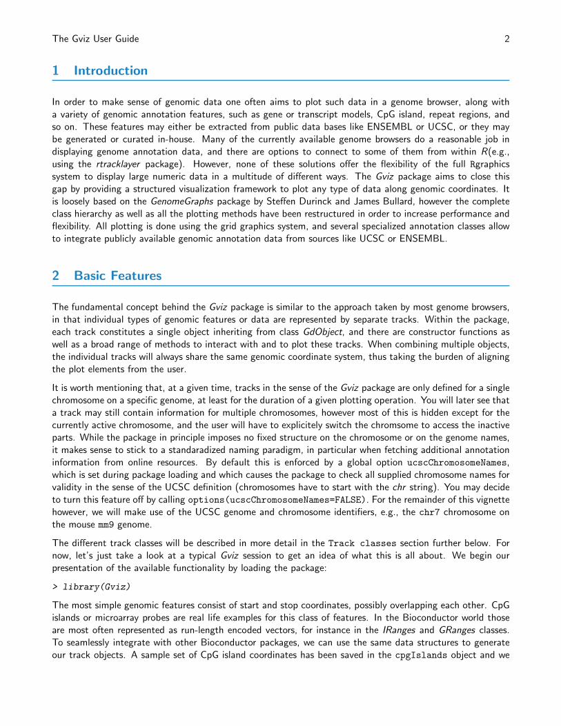
With our first track object being created we may now proceed to the plotting. There is a single functionplotTracks that handles all of this. As we will learn in the remainder of this vignette, plotTracks is quitepowerful and has a number of very useful additional arguments. For now we will keep things very simple andjust plot the single CpG islands annotation track.
> plotTracks(atrack)
CpG
As you can see, the resulting graph is not particularly spectacular. There is a title region showing the track’sname on a gray background on the left side of the plot and a data region showing the seven individual CpGislands on the right. This structure is similar for all the available track objects classes and it somewhat mimicksthe layout of the popular UCSC Genome Browser. If you are not happy with the default settings, the Gvizpackage offers a multitude of options to fine-tune the track appearance, which will be shown in the Plotting
Parameters section.
Appart from the relative distance of the Cpg islands, this visualization does not tell us much. One obviousnext step would be to indicate the genomic coordinates we are currently looking at in order to provide somereference. For this purpose, the Gviz package offers the GenomeAxisTrack class. Objects from the class canbe created using the constructor function of the same name.
> gtrack <- GenomeAxisTrack()
Since a GenomeAxisTrack object is always relative to the other tracks that are plotted, there is little need foradditional arguments. Essentially, the object just tells the plotTracks function to add a genomic axis to theplot. Nonetheless, it represent a separate annotation track just as the CpG island track does. We can passthis additional track on to plotTracks in the form of a list.
The Gviz User Guide 4
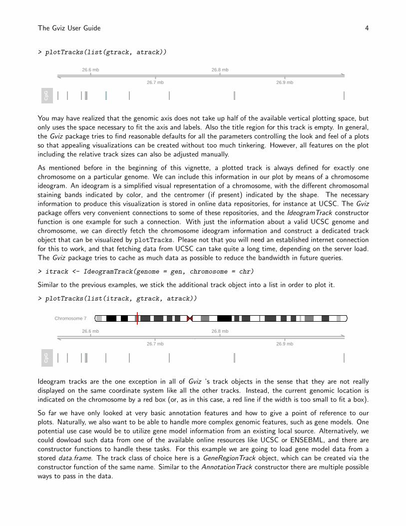
> plotTracks(list(gtrack, atrack))
26.6 mb
26.7 mb
26.8 mb
26.9 mb
CpG
You may have realized that the genomic axis does not take up half of the available vertical plotting space, butonly uses the space necessary to fit the axis and labels. Also the title region for this track is empty. In general,the Gviz package tries to find reasonable defaults for all the parameters controlling the look and feel of a plotsso that appealing visualizations can be created without too much tinkering. However, all features on the plotincluding the relative track sizes can also be adjusted manually.
As mentioned before in the beginning of this vignette, a plotted track is always defined for exactly onechromosome on a particular genome. We can include this information in our plot by means of a chromosomeideogram. An ideogram is a simplified visual representation of a chromosome, with the different chromosomalstaining bands indicated by color, and the centromer (if present) indicated by the shape. The necessaryinformation to produce this visualization is stored in online data repositories, for instance at UCSC. The Gvizpackage offers very convenient connections to some of these repositories, and the IdeogramTrack constructorfunction is one example for such a connection. With just the information about a valid UCSC genome andchromosome, we can directly fetch the chromosome ideogram information and construct a dedicated trackobject that can be visualized by plotTracks. Please not that you will need an established internet connectionfor this to work, and that fetching data from UCSC can take quite a long time, depending on the server load.The Gviz package tries to cache as much data as possible to reduce the bandwidth in future queries.
> itrack <- IdeogramTrack(genome = gen, chromosome = chr)
Similar to the previous examples, we stick the additional track object into a list in order to plot it.
> plotTracks(list(itrack, gtrack, atrack))
Chromosome 7
26.6 mb
26.7 mb
26.8 mb
26.9 mb
CpG
Ideogram tracks are the one exception in all of Gviz ’s track objects in the sense that they are not reallydisplayed on the same coordinate system like all the other tracks. Instead, the current genomic location isindicated on the chromosome by a red box (or, as in this case, a red line if the width is too small to fit a box).
So far we have only looked at very basic annotation features and how to give a point of reference to ourplots. Naturally, we also want to be able to handle more complex genomic features, such as gene models. Onepotential use case would be to utilize gene model information from an existing local source. Alternatively, wecould dowload such data from one of the available online resources like UCSC or ENSEBML, and there areconstructor functions to handle these tasks. For this example we are going to load gene model data from astored data.frame. The track class of choice here is a GeneRegionTrack object, which can be created via theconstructor function of the same name. Similar to the AnnotationTrack constructor there are multiple possibleways to pass in the data.
The Gviz User Guide 5
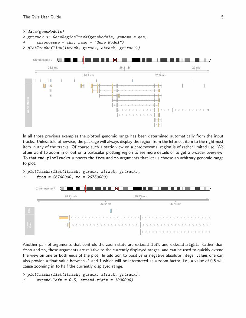
> data(geneModels)
> grtrack <- GeneRegionTrack(geneModels, genome = gen,
+ chromosome = chr, name = "Gene Model")
> plotTracks(list(itrack, gtrack, atrack, grtrack))
Chromosome 7
26.6 mb
26.7 mb
26.8 mb
26.9 mb
27 mb
Gen
e M
odel
In all those previous examples the plotted genomic range has been determined automatically from the inputtracks. Unless told otherwise, the package will always display the region from the leftmost item to the rightmostitem in any of the tracks. Of course such a static view on a chromosomal region is of rather limited use. Weoften want to zoom in or out on a particular plotting region to see more details or to get a broader overview.To that end, plotTracks supports the from and to arguments that let us choose an arbitrary genomic rangeto plot.
> plotTracks(list(itrack, gtrack, atrack, grtrack),
+ from = 26700000, to = 26750000)
Chromosome 7
26.71 mb
26.72 mb
26.73 mb
26.74 mb
CpG
Gen
eM
odel
Another pair of arguments that controls the zoom state are extend.left and extend.right. Rather thanfrom and to, those arguments are relative to the currently displayed ranges, and can be used to quickly extendthe view on one or both ends of the plot. In addition to positive or negative absolute integer values one canalso provide a float value between -1 and 1 which will be interpreted as a zoom factor, i.e., a value of 0.5 willcause zooming in to half the currently displayed range.
> plotTracks(list(itrack, gtrack, atrack, grtrack),
+ extend.left = 0.5, extend.right = 1000000)
The Gviz User Guide 6
Chromosome 7
26.5 mb
27 mb
27.5 mb
CpG
Gen
e M
odel
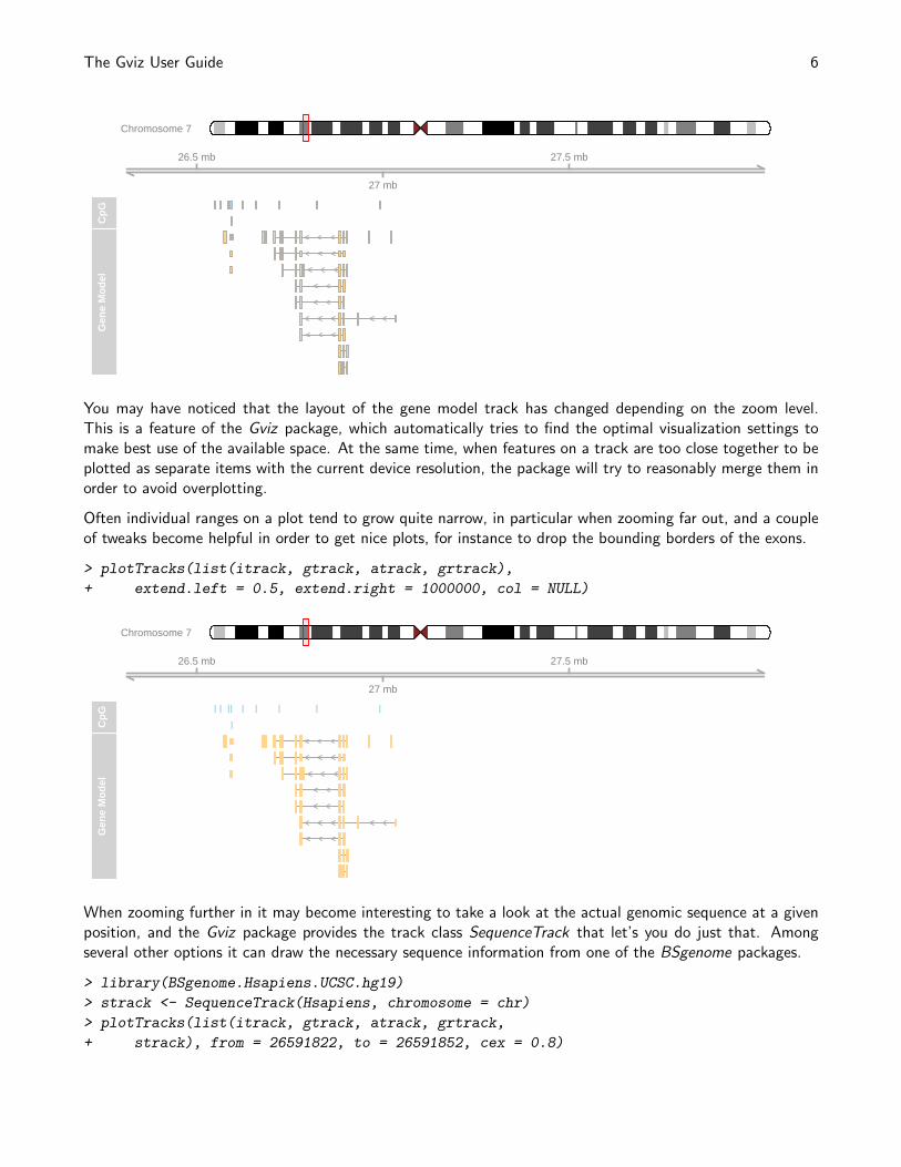
You may have noticed that the layout of the gene model track has changed depending on the zoom level.This is a feature of the Gviz package, which automatically tries to find the optimal visualization settings tomake best use of the available space. At the same time, when features on a track are too close together to beplotted as separate items with the current device resolution, the package will try to reasonably merge them inorder to avoid overplotting.
Often individual ranges on a plot tend to grow quite narrow, in particular when zooming far out, and a coupleof tweaks become helpful in order to get nice plots, for instance to drop the bounding borders of the exons.
> plotTracks(list(itrack, gtrack, atrack, grtrack),
+ extend.left = 0.5, extend.right = 1000000, col = NULL)
Chromosome 7
26.5 mb
27 mb
27.5 mb
CpG
Gen
e M
odel
When zooming further in it may become interesting to take a look at the actual genomic sequence at a givenposition, and the Gviz package provides the track class SequenceTrack that let’s you do just that. Amongseveral other options it can draw the necessary sequence information from one of the BSgenome packages.
> library(BSgenome.Hsapiens.UCSC.hg19)
> strack <- SequenceTrack(Hsapiens, chromosome = chr)
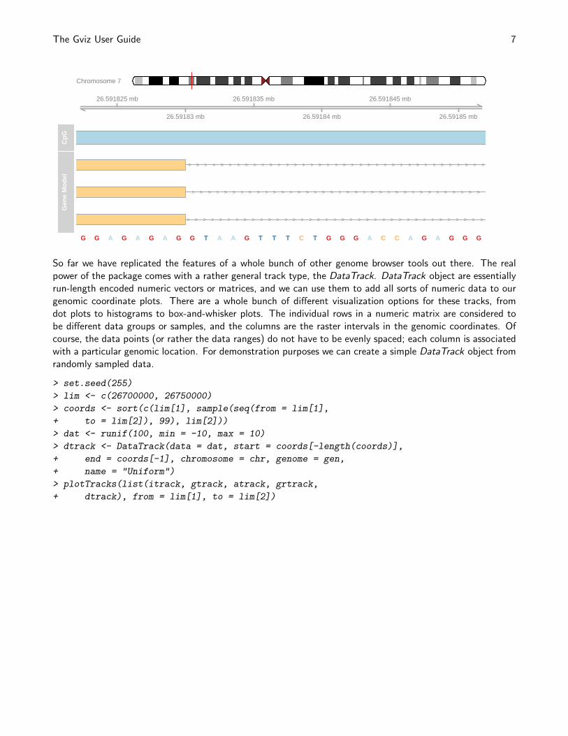
> plotTracks(list(itrack, gtrack, atrack, grtrack,
+ strack), from = 26591822, to = 26591852, cex = 0.8)
The Gviz User Guide 7
Chromosome 7
26.591825 mb
26.59183 mb
26.591835 mb
26.59184 mb
26.591845 mb
26.59185 mb
CpG
Gen
e M
odel
G G A G A G A G G T A A G T T T C T G G G A C C A G A G G G
So far we have replicated the features of a whole bunch of other genome browser tools out there. The realpower of the package comes with a rather general track type, the DataTrack. DataTrack object are essentiallyrun-length encoded numeric vectors or matrices, and we can use them to add all sorts of numeric data to ourgenomic coordinate plots. There are a whole bunch of different visualization options for these tracks, fromdot plots to histograms to box-and-whisker plots. The individual rows in a numeric matrix are considered tobe different data groups or samples, and the columns are the raster intervals in the genomic coordinates. Ofcourse, the data points (or rather the data ranges) do not have to be evenly spaced; each column is associatedwith a particular genomic location. For demonstration purposes we can create a simple DataTrack object fromrandomly sampled data.
> set.seed(255)
> lim <- c(26700000, 26750000)
> coords <- sort(c(lim[1], sample(seq(from = lim[1],
+ to = lim[2]), 99), lim[2]))
> dat <- runif(100, min = -10, max = 10)
> dtrack <- DataTrack(data = dat, start = coords[-length(coords)],
+ end = coords[-1], chromosome = chr, genome = gen,
+ name = "Uniform")
> plotTracks(list(itrack, gtrack, atrack, grtrack,
+ dtrack), from = lim[1], to = lim[2])
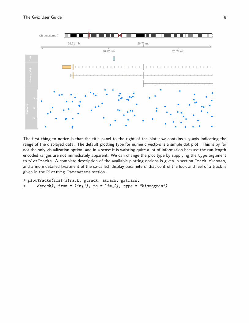
The Gviz User Guide 8
Chromosome 7
26.71 mb
26.72 mb
26.73 mb
26.74 mb
CpG
Gen
e M
odel
−5
0
5
Uni
form
●
●
●
●
●
●
●
● ●
●
●●
●
●
●
●
●
●
●
●
●
●●
●
●
●
●
●
●
●
●
●
●
●
●
●
●
●
●
●
●
●
●
●●
●
●
●
●
●
●
●
●
●
●
●
●
●
●
●
●
●
●
●
●
●
●
●
●
●
●
●
●
●
●
●
●●
●
●
●
●
●
●
●
●
● ●
●
●
●
● ●
●
●
●
●
●
●
●
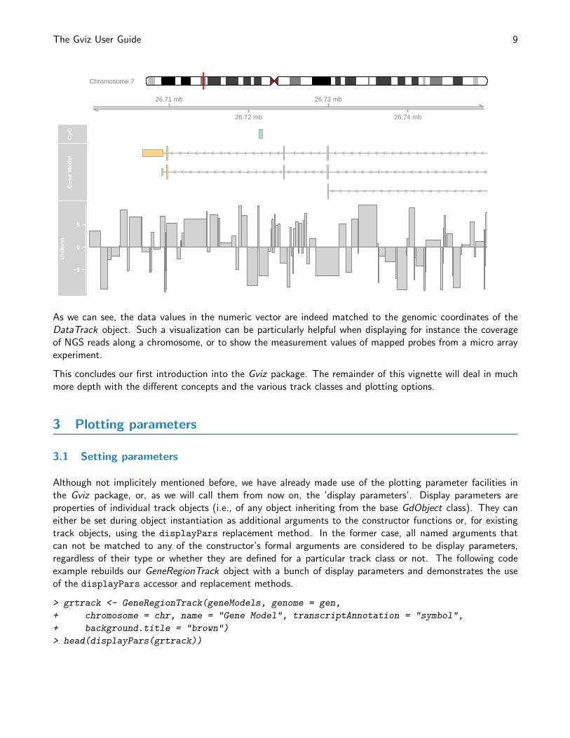
The first thing to notice is that the title panel to the right of the plot now contains a y-axis indicating therange of the displayed data. The default plotting type for numeric vectors is a simple dot plot. This is by farnot the only visualization option, and in a sense it is waisting quite a lot of information because the run-lengthencoded ranges are not immediately apparent. We can change the plot type by supplying the type argumentto plotTracks. A complete description of the available plotting options is given in section Track classes,and a more detailed treatment of the so-called ’display parameters’ that control the look and feel of a track isgiven in the Plotting Parameters section.
> plotTracks(list(itrack, gtrack, atrack, grtrack,
+ dtrack), from = lim[1], to = lim[2], type = "histogram")
The Gviz User Guide 9
Chromosome 7
26.71 mb
26.72 mb
26.73 mb
26.74 mb
CpG
Gen
e M
odel
−5
0
5
Uni
form
As we can see, the data values in the numeric vector are indeed matched to the genomic coordinates of theDataTrack object. Such a visualization can be particularly helpful when displaying for instance the coverageof NGS reads along a chromosome, or to show the measurement values of mapped probes from a micro arrayexperiment.
This concludes our first introduction into the Gviz package. The remainder of this vignette will deal in muchmore depth with the different concepts and the various track classes and plotting options.
3 Plotting parameters
3.1 Setting parameters
Although not implicitely mentioned before, we have already made use of the plotting parameter facilities inthe Gviz package, or, as we will call them from now on, the ’display parameters’. Display parameters areproperties of individual track objects (i.e., of any object inheriting from the base GdObject class). They caneither be set during object instantiation as additional arguments to the constructor functions or, for existingtrack objects, using the displayPars replacement method. In the former case, all named arguments thatcan not be matched to any of the constructor’s formal arguments are considered to be display parameters,regardless of their type or whether they are defined for a particular track class or not. The following codeexample rebuilds our GeneRegionTrack object with a bunch of display parameters and demonstrates the useof the displayPars accessor and replacement methods.
> grtrack <- GeneRegionTrack(geneModels, genome = gen,
+ chromosome = chr, name = "Gene Model", transcriptAnnotation = "symbol",
+ background.title = "brown")
> head(displayPars(grtrack))
The Gviz User Guide 10
$arrowHeadWidth
[1] 10
$arrowHeadMaxWidth
[1] 20
$col
[1] "darkgray"
$collapseTranscripts
[1] FALSE
$exonAnnotation
NULL
$fill
[1] "#FFD58A"
> displayPars(grtrack) <- list(background.panel = "#FFFEDB",
+ col = NULL)
> head(displayPars(grtrack))
$arrowHeadWidth
[1] 10
$arrowHeadMaxWidth
[1] 20
$col
NULL
$collapseTranscripts
[1] FALSE
$exonAnnotation
NULL
$fill
[1] "#FFD58A"
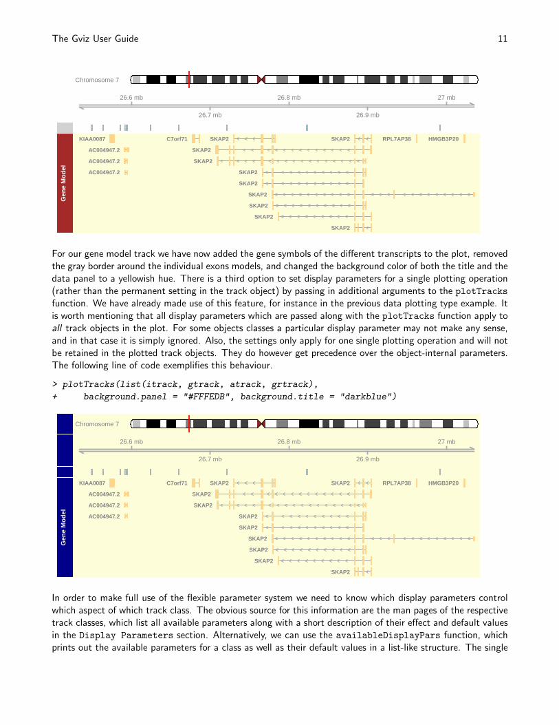
> plotTracks(list(itrack, gtrack, atrack, grtrack))
The Gviz User Guide 11
Chromosome 7
26.6 mb
26.7 mb
26.8 mb
26.9 mb
27 mb
Gen
e M
odel
KIAA0087
SKAP2
C7orf71 HMGB3P20
AC004947.2
AC004947.2
SKAP2
RPL7AP38
AC004947.2
SKAP2
SKAP2
SKAP2
SKAP2
SKAP2
SKAP2
SKAP2
SKAP2
For our gene model track we have now added the gene symbols of the different transcripts to the plot, removedthe gray border around the individual exons models, and changed the background color of both the title and thedata panel to a yellowish hue. There is a third option to set display parameters for a single plotting operation(rather than the permanent setting in the track object) by passing in additional arguments to the plotTracks
function. We have already made use of this feature, for instance in the previous data plotting type example. Itis worth mentioning that all display parameters which are passed along with the plotTracks function apply toall track objects in the plot. For some objects classes a particular display parameter may not make any sense,and in that case it is simply ignored. Also, the settings only apply for one single plotting operation and will notbe retained in the plotted track objects. They do however get precedence over the object-internal parameters.The following line of code exemplifies this behaviour.
> plotTracks(list(itrack, gtrack, atrack, grtrack),
+ background.panel = "#FFFEDB", background.title = "darkblue")
Chromosome 7
26.6 mb
26.7 mb
26.8 mb
26.9 mb
27 mb
Gen
e M
odel
KIAA0087
SKAP2
C7orf71 HMGB3P20
AC004947.2
AC004947.2
SKAP2
RPL7AP38
AC004947.2
SKAP2
SKAP2
SKAP2
SKAP2
SKAP2
SKAP2
SKAP2
SKAP2
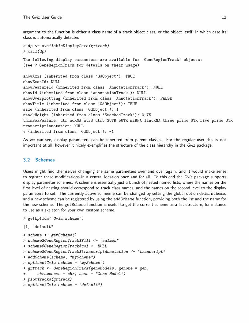
In order to make full use of the flexible parameter system we need to know which display parameters controlwhich aspect of which track class. The obvious source for this information are the man pages of the respectivetrack classes, which list all available parameters along with a short description of their effect and default valuesin the Display Parameters section. Alternatively, we can use the availableDisplayPars function, whichprints out the available parameters for a class as well as their default values in a list-like structure. The single
The Gviz User Guide 12
argument to the function is either a class name of a track object class, or the object itself, in which case itsclass is automatically detected.
> dp <- availableDisplayPars(grtrack)
> tail(dp)
The following display parameters are available for 'GeneRegionTrack' objects:
(see ? GeneRegionTrack for details on their usage)
showAxis (inherited from class 'GdObject'): TRUE
showExonId: NULL
showFeatureId (inherited from class 'AnnotationTrack'): NULL
showId (inherited from class 'AnnotationTrack'): NULL
showOverplotting (inherited from class 'AnnotationTrack'): FALSE
showTitle (inherited from class 'GdObject'): TRUE
size (inherited from class 'GdObject'): 1
stackHeight (inherited from class 'StackedTrack'): 0.75
thinBoxFeature: utr ncRNA utr3 utr5 3UTR 5UTR miRNA lincRNA three_prime_UTR five_prime_UTR
transcriptAnnotation: NULL
v (inherited from class 'GdObject'): -1
As we can see, display parameters can be inherited from parent classes. For the regular user this is notimportant at all, however it nicely exemplifies the structure of the class hierarchy in the Gviz package.
3.2 Schemes
Users might find themselves changing the same parameters over and over again, and it would make senseto register these modifications in a central location once and for all. To this end the Gviz package supportsdisplay parameter schemes. A scheme is essentially just a bunch of nested named lists, where the names on thefirst level of nesting should correspond to track class names, and the names on the second level to the displayparameters to set. The currently active schmeme can be changed by setting the global option Gviz.scheme,and a new scheme can be registered by using the addScheme function, providing both the list and the name forthe new scheme. The getScheme function is useful to get the current scheme as a list structure, for instanceto use as a skeleton for your own custom scheme.
> getOption("Gviz.scheme")
[1] "default"
> scheme <- getScheme()
> scheme$GeneRegionTrack$fill <- "salmon"
> scheme$GeneRegionTrack$col <- NULL
> scheme$GeneRegionTrack$transcriptAnnotation <- "transcript"
> addScheme(scheme, "myScheme")
> options(Gviz.scheme = "myScheme")
> grtrack <- GeneRegionTrack(geneModels, genome = gen,
+ chromosome = chr, name = "Gene Model")
> plotTracks(grtrack)
> options(Gviz.scheme = "default")
The Gviz User Guide 13
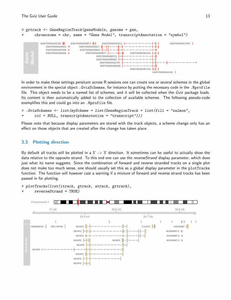
> grtrack <- GeneRegionTrack(geneModels, genome = gen,
+ chromosome = chr, name = "Gene Model", transcriptAnnotation = "symbol")
Gen
eM
odel
ENST00000242109ENST00000345317
ENST00000409974 ENST00000417997ENST00000420912
ENST00000430426
ENST00000432747
ENST00000441433
ENST00000457000
ENST00000468712ENST00000481204
ENST00000487720
ENST00000489977
ENST00000490456
ENST00000495802
ENST00000497511
ENST00000539623
In order to make these settings persitant across R sessions one can create one or several schemes in the globalenvironment in the special object .GvizSchemes, for instance by putting the necessary code in the .Rprofile
file. This object needs to be a named list of schemes, and it will be collected when the Gviz package loads.Its content is then automatically added to the collection of available schemes. The following pseudo-codeexemplifies this and could go into an .Rprofile file.
> .GvizSchemes <- list(myScheme = list(GeneRegionTrack = list(fill = "salmon",
+ col = NULL, transcriptAnnotation = "transcript")))
Please note that because display parameters are stored with the track objects, a scheme change only has aneffect on those objects that are created after the change has taken place.
3.3 Plotting direction
By default all tracks will be plotted in a 5’ -> 3’ direction. It sometimes can be useful to actually show thedata relative to the opposite strand. To this end one can use the reverseStrand display parameter, which doesjust what its name suggests. Since the combination of forward and reverse stranded tracks on a single plotdoes not make too much sense, one should usually set this as a global display parameter in the plotTracks
function. The function will however cast a warning if a mixture of forward and reverse strand tracks has beenpassed in for plotting.
> plotTracks(list(itrack, gtrack, atrack, grtrack),
+ reverseStrand = TRUE)
Chromosome 7
26.6 mb
26.7 mb
26.8 mb
26.9 mb
27 mb
Gen
e M
odel
KIAA0087
SKAP2
C7orf71HMGB3P20
AC004947.2
AC004947.2
SKAP2
RPL7AP38
AC004947.2
SKAP2
SKAP2
SKAP2 SKAP2
SKAP2
SKAP2
SKAP2
SKAP2
The Gviz User Guide 14
As you can see, the fact that the data has been plotted on the reverse strand is also reflected in the GenomeAxistrack.
4 Track classes
In this section we will highlight all of the available annotation track classes in the Gviz package. For thecomplete reference of all the nuts and bolts, including all the avaialable methods, please see the respectiveclass man pages. We will try to keep this vignette up to date, but in cases of discrepancies between here andthe man pages you should assume the latter to be correct.
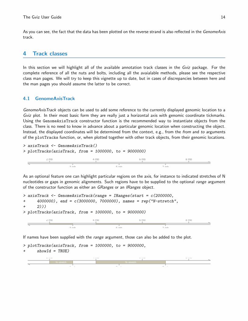
4.1 GenomeAxisTrack
GenomeAxisTrack objects can be used to add some reference to the currently displayed genomic location to aGviz plot. In their most basic form they are really just a horizontal axis with genomic coordinate tickmarks.Using the GenomeAxisTrack constructor function is the recommended way to instantiate objects from theclass. There is no need to know in advance about a particular genomic location when constructing the object.Instead, the displayed coordinates will be determined from the context, e.g., from the from and to argumentsof the plotTracks function, or, when plotted together with other track objects, from their genomic locations.
> axisTrack <- GenomeAxisTrack()
> plotTracks(axisTrack, from = 1000000, to = 9000000)
2 mb
3 mb
4 mb
5 mb
6 mb
7 mb
8 mb
As an optional feature one can highlight particular regions on the axis, for instance to indicated stretches of Nnucleotides or gaps in genomic alignments. Such regions have to be supplied to the optional range argumentof the constructor function as either an GRanges or an IRanges object.
> axisTrack <- GenomeAxisTrack(range = IRanges(start = c(2000000,
+ 4000000), end = c(3000000, 7000000), names = rep("N-stretch",
+ 2)))
> plotTracks(axisTrack, from = 1000000, to = 9000000)
2 mb
3 mb
4 mb
5 mb
6 mb
7 mb
8 mb
If names have been supplied with the range argument, those can also be added to the plot.
> plotTracks(axisTrack, from = 1000000, to = 9000000,
+ showId = TRUE)
N−stretch N−stretch
2 mb
3 mb
4 mb
5 mb
6 mb
7 mb
8 mb
The Gviz User Guide 15
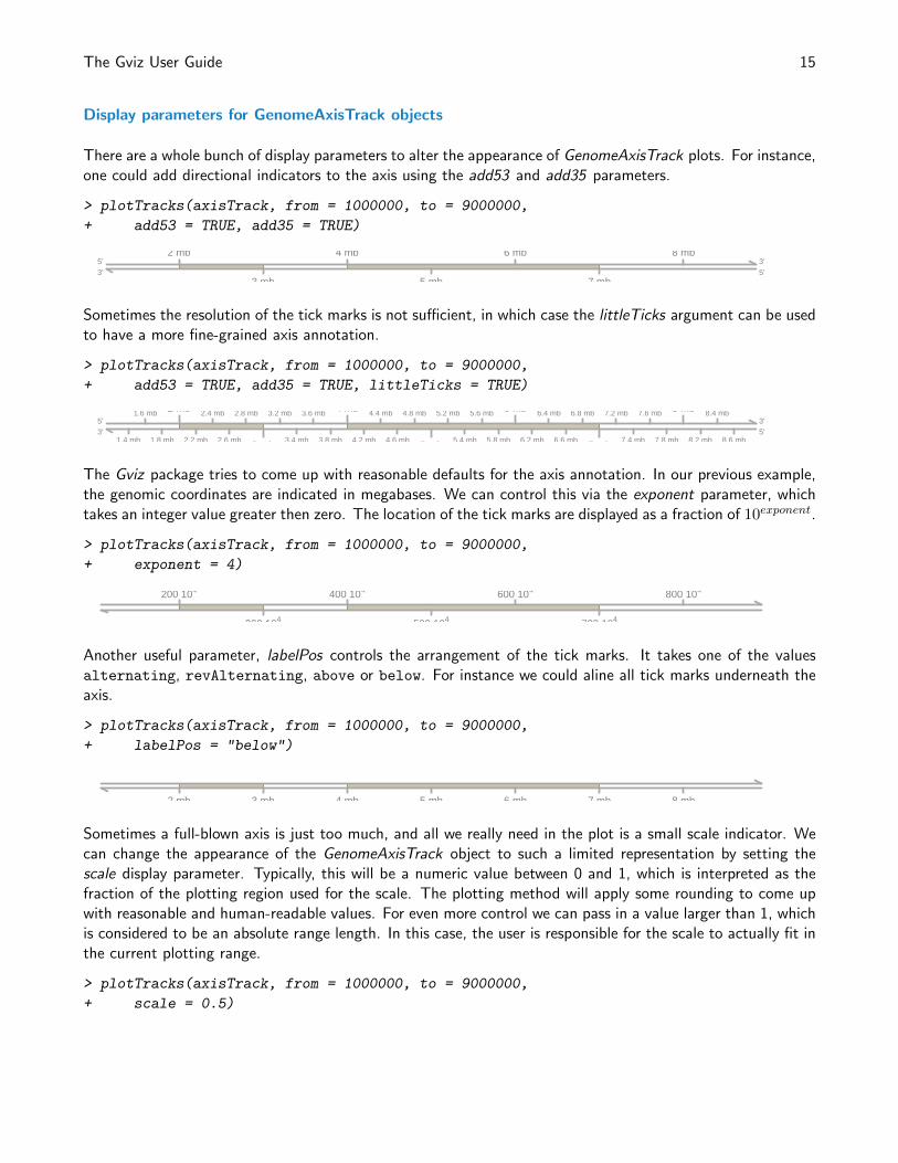
Display parameters for GenomeAxisTrack objects
There are a whole bunch of display parameters to alter the appearance of GenomeAxisTrack plots. For instance,one could add directional indicators to the axis using the add53 and add35 parameters.
> plotTracks(axisTrack, from = 1000000, to = 9000000,
+ add53 = TRUE, add35 = TRUE)
2 mb
3 mb
4 mb
5 mb
6 mb
7 mb
8 mb5' 3'3' 5'
Sometimes the resolution of the tick marks is not sufficient, in which case the littleTicks argument can be usedto have a more fine-grained axis annotation.
> plotTracks(axisTrack, from = 1000000, to = 9000000,
+ add53 = TRUE, add35 = TRUE, littleTicks = TRUE)
2 mb
3 mb
4 mb
5 mb
6 mb
7 mb
8 mb
1.4 mb
1.6 mb
1.8 mb 2.2 mb
2.4 mb
2.6 mb
2.8 mb 3.2 mb
3.4 mb
3.6 mb
3.8 mb 4.2 mb
4.4 mb
4.6 mb
4.8 mb 5.2 mb
5.4 mb
5.6 mb
5.8 mb 6.2 mb
6.4 mb
6.6 mb
6.8 mb 7.2 mb
7.4 mb
7.6 mb
7.8 mb 8.2 mb
8.4 mb
8.6 mb
5' 3'3' 5'
The Gviz package tries to come up with reasonable defaults for the axis annotation. In our previous example,the genomic coordinates are indicated in megabases. We can control this via the exponent parameter, whichtakes an integer value greater then zero. The location of the tick marks are displayed as a fraction of 10exponent.
> plotTracks(axisTrack, from = 1000000, to = 9000000,
+ exponent = 4)
200 104
300 104
400 104
500 104
600 104
700 104
800 104
Another useful parameter, labelPos controls the arrangement of the tick marks. It takes one of the valuesalternating, revAlternating, above or below. For instance we could aline all tick marks underneath theaxis.
> plotTracks(axisTrack, from = 1000000, to = 9000000,
+ labelPos = "below")
2 mb 3 mb 4 mb 5 mb 6 mb 7 mb 8 mb
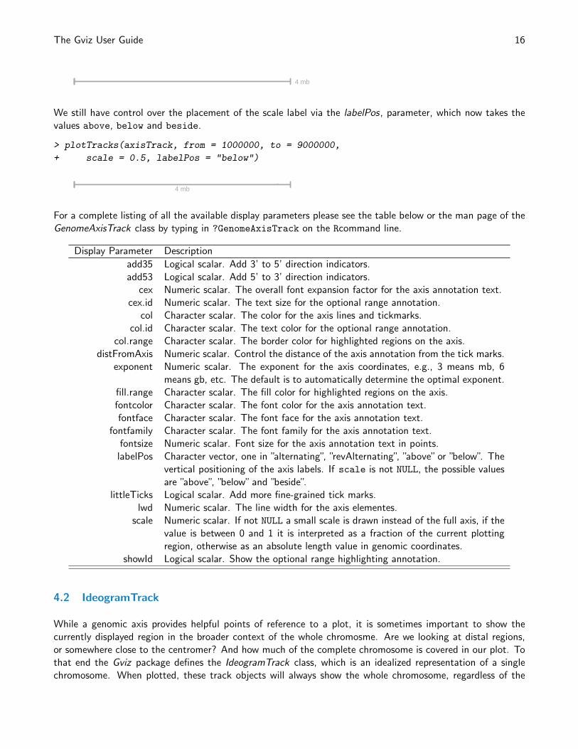
Sometimes a full-blown axis is just too much, and all we really need in the plot is a small scale indicator. Wecan change the appearance of the GenomeAxisTrack object to such a limited representation by setting thescale display parameter. Typically, this will be a numeric value between 0 and 1, which is interpreted as thefraction of the plotting region used for the scale. The plotting method will apply some rounding to come upwith reasonable and human-readable values. For even more control we can pass in a value larger than 1, whichis considered to be an absolute range length. In this case, the user is responsible for the scale to actually fit inthe current plotting range.
> plotTracks(axisTrack, from = 1000000, to = 9000000,
+ scale = 0.5)
The Gviz User Guide 16
4 mb
We still have control over the placement of the scale label via the labelPos, parameter, which now takes thevalues above, below and beside.
> plotTracks(axisTrack, from = 1000000, to = 9000000,
+ scale = 0.5, labelPos = "below")
4 mb
For a complete listing of all the available display parameters please see the table below or the man page of theGenomeAxisTrack class by typing in ?GenomeAxisTrack on the Rcommand line.
Display Parameter Description
add35 Logical scalar. Add 3’ to 5’ direction indicators.add53 Logical scalar. Add 5’ to 3’ direction indicators.
cex Numeric scalar. The overall font expansion factor for the axis annotation text.cex.id Numeric scalar. The text size for the optional range annotation.
col Character scalar. The color for the axis lines and tickmarks.col.id Character scalar. The text color for the optional range annotation.
col.range Character scalar. The border color for highlighted regions on the axis.distFromAxis Numeric scalar. Control the distance of the axis annotation from the tick marks.
exponent Numeric scalar. The exponent for the axis coordinates, e.g., 3 means mb, 6means gb, etc. The default is to automatically determine the optimal exponent.
fill.range Character scalar. The fill color for highlighted regions on the axis.fontcolor Character scalar. The font color for the axis annotation text.fontface Character scalar. The font face for the axis annotation text.
fontfamily Character scalar. The font family for the axis annotation text.fontsize Numeric scalar. Font size for the axis annotation text in points.
labelPos Character vector, one in ”alternating”, ”revAlternating”, ”above” or ”below”. Thevertical positioning of the axis labels. If scale is not NULL, the possible valuesare ”above”, ”below” and ”beside”.
littleTicks Logical scalar. Add more fine-grained tick marks.lwd Numeric scalar. The line width for the axis elementes.
scale Numeric scalar. If not NULL a small scale is drawn instead of the full axis, if thevalue is between 0 and 1 it is interpreted as a fraction of the current plottingregion, otherwise as an absolute length value in genomic coordinates.
showId Logical scalar. Show the optional range highlighting annotation.
4.2 IdeogramTrack
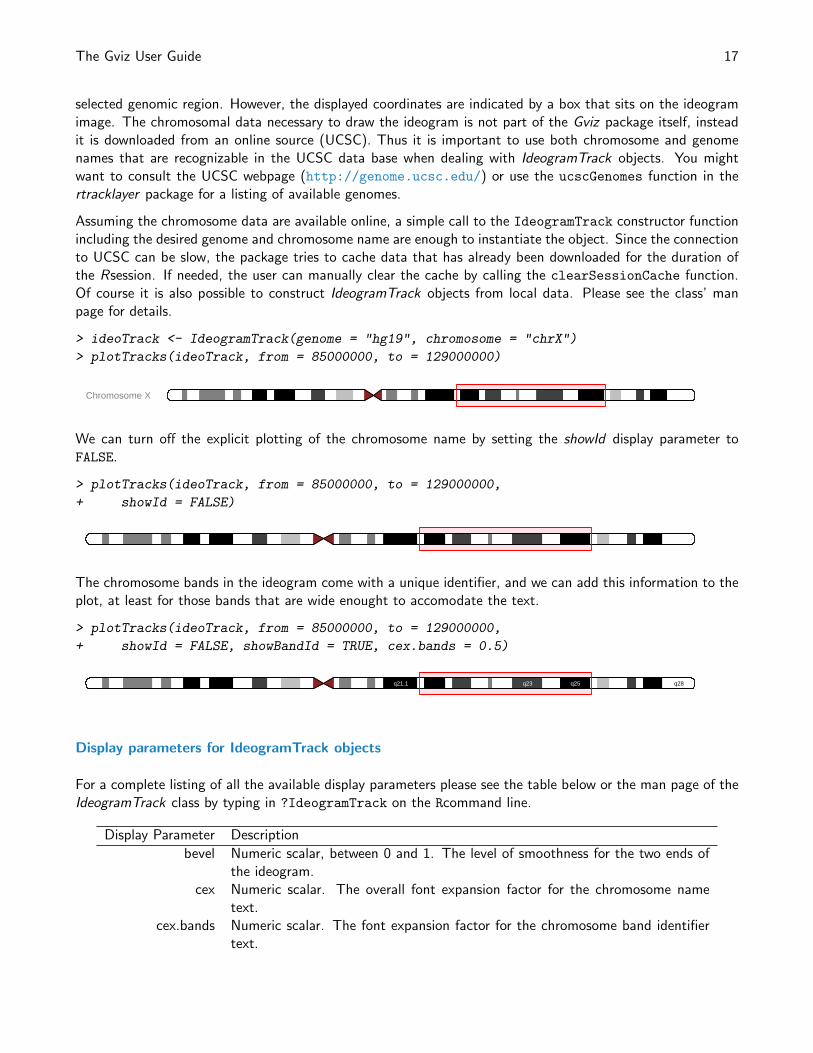
While a genomic axis provides helpful points of reference to a plot, it is sometimes important to show thecurrently displayed region in the broader context of the whole chromosme. Are we looking at distal regions,or somewhere close to the centromer? And how much of the complete chromosome is covered in our plot. Tothat end the Gviz package defines the IdeogramTrack class, which is an idealized representation of a singlechromosome. When plotted, these track objects will always show the whole chromosome, regardless of the
The Gviz User Guide 17
selected genomic region. However, the displayed coordinates are indicated by a box that sits on the ideogramimage. The chromosomal data necessary to draw the ideogram is not part of the Gviz package itself, insteadit is downloaded from an online source (UCSC). Thus it is important to use both chromosome and genomenames that are recognizable in the UCSC data base when dealing with IdeogramTrack objects. You mightwant to consult the UCSC webpage (http://genome.ucsc.edu/) or use the ucscGenomes function in thertracklayer package for a listing of available genomes.
Assuming the chromosome data are available online, a simple call to the IdeogramTrack constructor functionincluding the desired genome and chromosome name are enough to instantiate the object. Since the connectionto UCSC can be slow, the package tries to cache data that has already been downloaded for the duration ofthe Rsession. If needed, the user can manually clear the cache by calling the clearSessionCache function.Of course it is also possible to construct IdeogramTrack objects from local data. Please see the class’ manpage for details.
> ideoTrack <- IdeogramTrack(genome = "hg19", chromosome = "chrX")
> plotTracks(ideoTrack, from = 85000000, to = 129000000)
Chromosome X
We can turn off the explicit plotting of the chromosome name by setting the showId display parameter toFALSE.
> plotTracks(ideoTrack, from = 85000000, to = 129000000,
+ showId = FALSE)
The chromosome bands in the ideogram come with a unique identifier, and we can add this information to theplot, at least for those bands that are wide enought to accomodate the text.
> plotTracks(ideoTrack, from = 85000000, to = 129000000,
+ showId = FALSE, showBandId = TRUE, cex.bands = 0.5)
q21.1 q23 q25 q28
Display parameters for IdeogramTrack objects
For a complete listing of all the available display parameters please see the table below or the man page of theIdeogramTrack class by typing in ?IdeogramTrack on the Rcommand line.
Display Parameter Description
bevel Numeric scalar, between 0 and 1. The level of smoothness for the two ends ofthe ideogram.
cex Numeric scalar. The overall font expansion factor for the chromosome nametext.
cex.bands Numeric scalar. The font expansion factor for the chromosome band identifiertext.
The Gviz User Guide 18
col Character scalar. The border color used for the highlighting of the currentlydisplayed genomic region.
fill Character scalar. The fill color used for the highlighting of the currently displayedgenomic region.
fontcolor Character scalar. The font color for the chromosome name text.fontface Character scalar. The font face for the chromosome name text.
fontfamily Character scalar. The font family for the chromosome name text.fontsize Numeric scalar. The font size for the chromosome name text.
lty Character or integer scalar. The line type used for the highlighting of the cur-rently displayed genomic region.
lwd Numeric scalar. The line width used for the highlighting of the currently dis-played genomic region.
outline Logical scalar. Add borders to the individual chromosome staining bands.showBandId Logical scalar. Show the identifier for the chromosome bands if there is space
for it.showId Logical scalar. Indicate the chromosome name next to the ideogram.
4.3 DataTrack
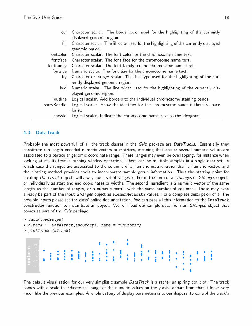
Probably the most powerfull of all the track classes in the Gviz package are DataTracks. Essentially theyconstitute run-length encoded numeric vectors or matrices, meaning that one or several numeric values areassociated to a particular genomic coordinate range. These ranges may even be overlapping, for instance whenlooking at results from a running window operation. There can be multiple samples in a single data set, inwhich case the ranges are associated to the columns of a numeric matrix rather than a numeric vector, andthe plotting method provides tools to incoorporate sample group information. Thus the starting point forcreating DataTrack objects will always be a set of ranges, either in the form of an IRanges or GRanges object,or individually as start and end coordinates or widths. The second ingredient is a numeric vector of the samelength as the number of ranges, or a numeric matrix with the same number of columns. Those may evenalready be part of the input GRanges object as elemenMetadata values. For a complete description of all thepossible inputs please see the class’ online documentation. We can pass all this information to the DataTrack
constructor function to instantiate an object. We will load our sample data from an GRanges object thatcomes as part of the Gviz package.
> data(twoGroups)
> dTrack <- DataTrack(twoGroups, name = "uniform")
> plotTracks(dTrack)
−20
−10
0
10
20
unifo
rm
●●
●
●
●●
●
●
●●
●
●●
●
●●●
● ●
●
●
●
●
●●
●
●
●
●
●
●
●
●●
●
●
●
●
●
●
●● ●
●
●
●
●
●
●●
●●
●●
●
●
●
●
●
●
●
●
●
●●
●
●
●
●
●
●●
●
●●
●●
●
●
●
●
●
●●
●
●●
●
●
●
●●
●
●●
●
●
●
●
●
●
●
●
●●●●
●
●
●●●
●●
●●
●●
●●
●
●●
●
●
●
●●
●
●
●
●
●●●
●
●
● ●
●●
●
●●
●
●
●
●
●
●
The default visualization for our very simplistic sample DataTrack is a rather unispiring dot plot. The trackcomes with a scale to indicate the range of the numeric values on the y-axis, appart from that it looks verymuch like the previous examples. A whole battery of display parameters is to our disposal to control the track’s
The Gviz User Guide 19
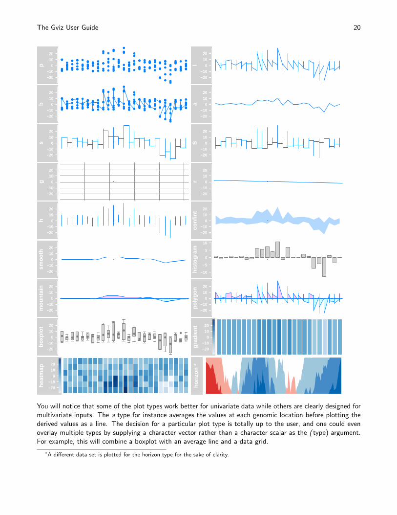
look and feel. The most important one is the type parameter. It determines the type of plot to use and takesone or several of the following values:
Value Type
p dot plotl lines plot
b dot and lines plota lines plot of average (i.e., mean) valuess stair steps (horizontal first)S stair steps (vertical first)g add grid linesr add linear regression lineh histogram lines
confint confidence intervals for average valuessmooth add loess curve
histogram histogram (bar width equal to range with)mountain ’mountain-type’ plot relative to a baseline
polygon ’polygon-type’ plot relative to a baselineboxplot box and whisker plot
gradient false color image of the summarized valuesheatmap false color image of the individual values
horizon Horizon plot indicating magnitude and direction of a change relative to a baseline
Displayed below are the same sample data as before but plotted with the different type settings:
The Gviz User Guide 20
−20−10
01020
p
●●
●
●
●●
●
●
●●
●
● ●
●
●●●
● ●
●
●
●
●
●●
●
●
●
●
●●
●
●●
●
●
●
●
●
●
●● ●
●
●
●
●
●
●●
●●
●●
●
●
●
●
●
●
●
●●
●●
●
●
●
●
●
●●
●
●●
●●
●
●
●●
●
●●
●
●●
●●
●
●●
●
●●
●
●●
●●
●
●
●
●●●●
●●
●●●
●●
●●
●●
●●
●
●●
●
●
●
●●
●
●
●
●
●●●
●
●
● ●●●
●
●●
●●
●
●
●
●
−20−10
01020
l
−20−10
01020
b
●●
●
●
●●
●
●
●●
●
● ●
●
●●●
● ●
●
●
●
●
●●
●
●
●
●
●●
●
●●
●
●
●
●
●
●
●● ●
●
●
●
●
●
●●
●●
●●
●
●
●
●
●
●
●
●●
●●
●
●
●
●
●
●●
●
●●
●●
●
●
●●
●
●●
●
●●
●●
●
●●
●
●●
●
●●
●●
●
●
●
●●●●
●●
●●●
●●
●●
●●
●●
●
●●
●
●
●
●●
●
●
●
●
●●●
●
●
● ●●●
●
●●
●●
●
●
●
●
−20−10
01020
a
−20−10
01020
s
−20−10
01020
S−20−10
01020
g
−20−10
01020
r
−20−10
01020
h
−20−10
01020
conf
int
−20−10
01020
smoo
th
−10
−5
0
5
10
hist
ogra
m
−20−10
01020
mou
ntai
n
−20−10
01020
poly
gon
−20−10
01020
boxp
lot
●● ●
● ● ● ●●
●● ● ●
●
●
●
●●
●
●
●
●
●
●
●
●
●
−20−10
01020
grad
ient
−20−10
01020
heat
map
horiz
on *
You will notice that some of the plot types work better for univariate data while others are clearly designed formultivariate inputs. The a type for instance averages the values at each genomic location before plotting thederived values as a line. The decision for a particular plot type is totally up to the user, and one could evenoverlay multiple types by supplying a character vector rather than a character scalar as the ( type) argument.For example, this will combine a boxplot with an average line and a data grid.
∗A different data set is plotted for the horizon type for the sake of clarity.
The Gviz User Guide 21
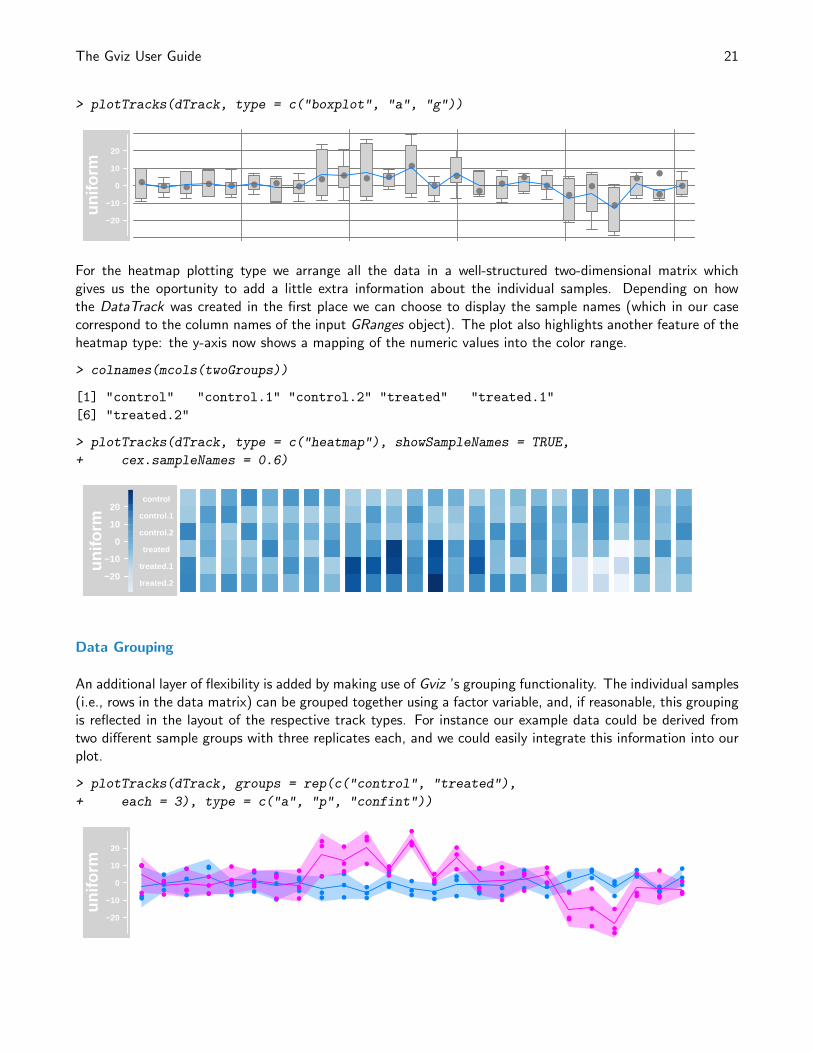
> plotTracks(dTrack, type = c("boxplot", "a", "g"))
−20
−10
0
10
20
unifo
rm
●● ● ● ● ● ● ●
●● ● ●
●
●
●
●●
●
●
●
●
●
●
●
●
●
For the heatmap plotting type we arrange all the data in a well-structured two-dimensional matrix whichgives us the oportunity to add a little extra information about the individual samples. Depending on howthe DataTrack was created in the first place we can choose to display the sample names (which in our casecorrespond to the column names of the input GRanges object). The plot also highlights another feature of theheatmap type: the y-axis now shows a mapping of the numeric values into the color range.
> colnames(mcols(twoGroups))
[1] "control" "control.1" "control.2" "treated" "treated.1"
[6] "treated.2"
> plotTracks(dTrack, type = c("heatmap"), showSampleNames = TRUE,
+ cex.sampleNames = 0.6)
treated.2
treated.1
treated
control.2
control.1
control
−20
−10
0
10
20
unifo
rm
Data Grouping
An additional layer of flexibility is added by making use of Gviz ’s grouping functionality. The individual samples(i.e., rows in the data matrix) can be grouped together using a factor variable, and, if reasonable, this groupingis reflected in the layout of the respective track types. For instance our example data could be derived fromtwo different sample groups with three replicates each, and we could easily integrate this information into ourplot.
> plotTracks(dTrack, groups = rep(c("control", "treated"),
+ each = 3), type = c("a", "p", "confint"))
−20
−10
0
10
20
unifo
rm
●●
●
●
●
●
●
●
●
●
●
●
●
●
●
●
●
●
●
●
●
●
●
●
●●
●
●
●
●
●
●
●
●
●
●●
●●
●
●
●●
●●
●●
●
●
●
●
●
●●
●
●●
●●
●
●
●●
●●
●
●●●
●
●●
●
●
●
●
●●
●
●
●
●●
●
●
●
●
●
●
●●
●
●
●
●●
●
●
●
●
●●
●
●
●
●●
●
●
●●
●●
●
●
●●
●
●
●
●●
● ●
●
● ●●
●
●
●●
●
●●
●
●
●
●
●
●
●
●
●
●
●●●
●
●
The Gviz User Guide 22
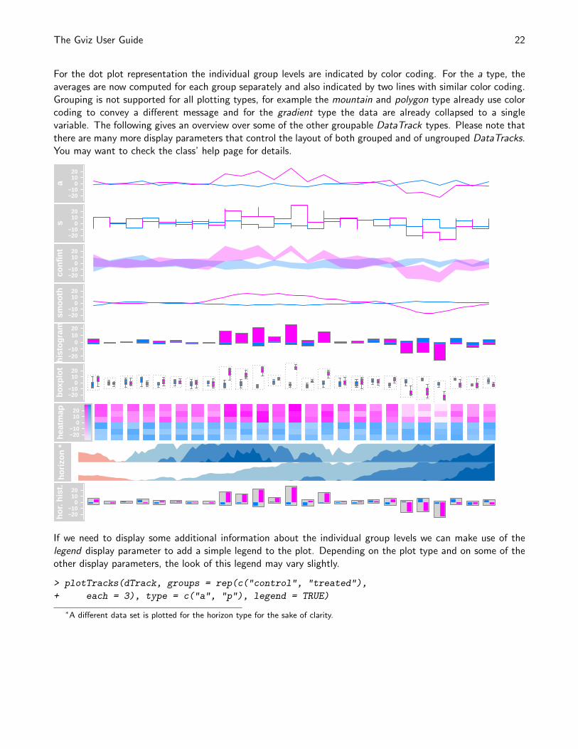
For the dot plot representation the individual group levels are indicated by color coding. For the a type, theaverages are now computed for each group separately and also indicated by two lines with similar color coding.Grouping is not supported for all plotting types, for example the mountain and polygon type already use colorcoding to convey a different message and for the gradient type the data are already collapsed to a singlevariable. The following gives an overview over some of the other groupable DataTrack types. Please note thatthere are many more display parameters that control the layout of both grouped and of ungrouped DataTracks.You may want to check the class’ help page for details.
−20−10
01020
a
−20−10
01020
s
−20−10
01020
conf
int
−20−10
01020
smoo
th
−20−10
01020
hist
ogra
m
−20−10
01020
boxp
lot
●
●●
●
●●
●●
●
●
●
●
● ●
●
●●
●
●
●●
●
●
●
●
●
●
●●
●●
●
●
●
●
●
●
●
●
●
●
● ● ●
●
●
●
●●
●
−20−10
01020
heat
map
horiz
on *
−20−10
01020
hor.
hist
.
If we need to display some additional information about the individual group levels we can make use of thelegend display parameter to add a simple legend to the plot. Depending on the plot type and on some of theother display parameters, the look of this legend may vary slightly.
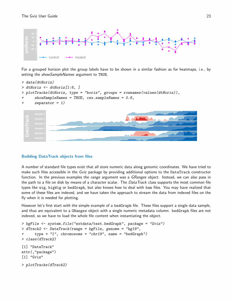
> plotTracks(dTrack, groups = rep(c("control", "treated"),
+ each = 3), type = c("a", "p"), legend = TRUE)
∗A different data set is plotted for the horizon type for the sake of clarity.
The Gviz User Guide 23
−20
−10
0
10
20
unifo
rm
●●
●
●
●
●●
●
●
●
●
●
●
●
●
●
●
●●
●
●●
●
●
●●
●
●
●
●
●
●●
●
●
●●
●●
●
●●
●
●●
●●
●
●
●
●
●
●●
●
●●
●●
●
●
●●
●●
●
●●●
●●●
●●
●
●
●●
●
●
●
●●
●
●
●
●
●
●
●●
●
●
●
●●●
●
●
●
●●
●
●
●
●●
●
●
●●
●●
●
●
●●
●●
●
●●
● ●
●
● ●●
●
●
●●
●
●●
●
●
●
●
●
●
●
●
●
●
●●●
●
●
● control ● treated
For a grouped horizon plot the group labels have to be shown in a similar fashion as for heatmaps, i.e., bysetting the showSampleNames argument to TRUE.
> data(dtHoriz)
> dtHoriz <- dtHoriz[1:6, ]
> plotTracks(dtHoriz, type = "horiz", groups = rownames(values(dtHoriz)),
+ showSampleNames = TRUE, cex.sampleNames = 0.6,
+ separator = 1)
Sample 1
Sample 2
Sample 3
Sample 4
Sample 5
Sample 6
Dat
aTra
ck
Building DataTrack objects from files
A number of standard file types exist that all store numeric data along genomic coordinates. We have tried tomake such files accessible in the Gviz package by providing additional options to the DataTrack constructorfunction. In the previous examples the range argument was a GRanges object. Instead, we can also pass inthe path to a file on disk by means of a character scalar. The DataTrack class supports the most common filetypes like wig, bigWig or bedGraph, but also knows how to deal with bam files. You may have realized thatsome of these files are indexed, and we have taken the approach to stream the data from indexed files on thefly when it is needed for plotting.
However let’s first start with the simple example of a bedGraph file. These files support a single data sample,and thus are equivalent to a GRanges object with a single numeric metadata column. bedGraph files are notindexed, so we have to load the whole file content when instantiating the object.
> bgFile <- system.file("extdata/test.bedGraph", package = "Gviz")
> dTrack2 <- DataTrack(range = bgFile, genome = "hg19",
+ type = "l", chromosome = "chr19", name = "bedGraph")
> class(dTrack2)
[1] "DataTrack"
attr(,"package")
[1] "Gviz"
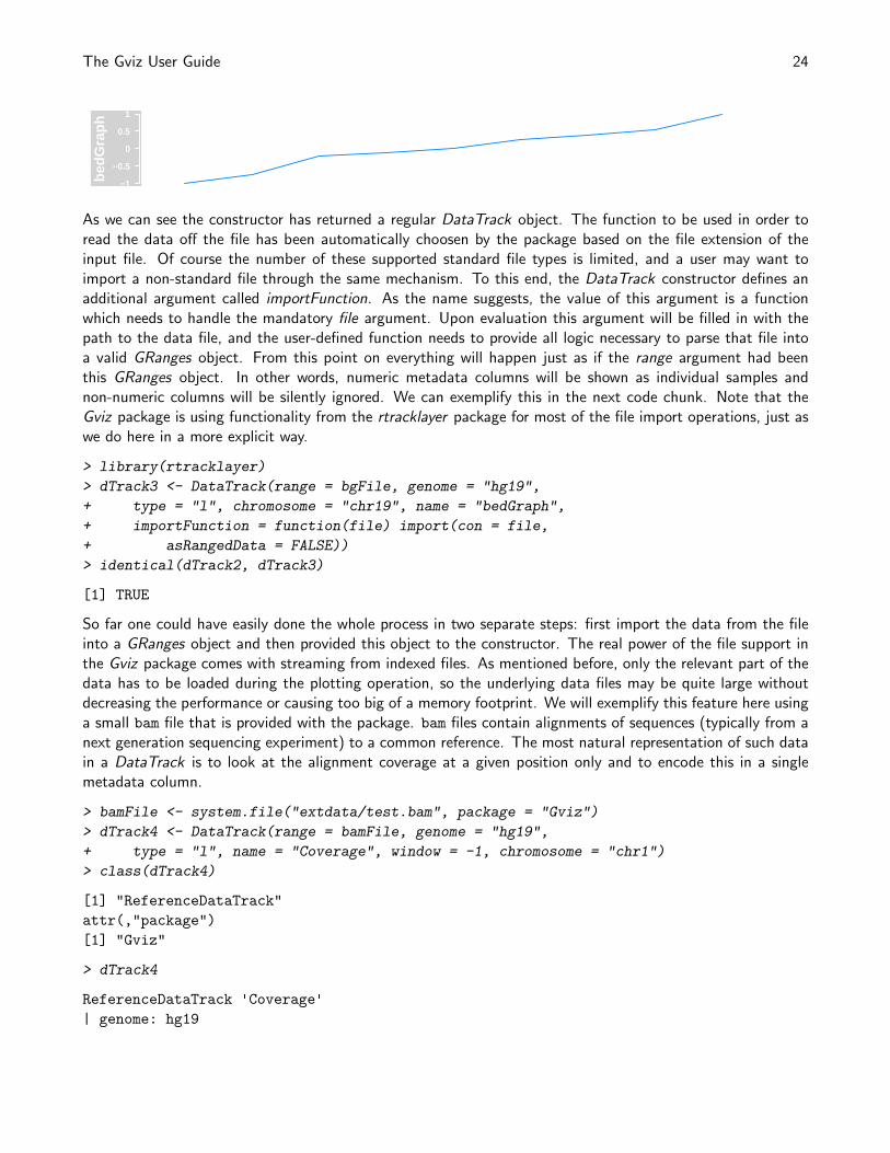
> plotTracks(dTrack2)
The Gviz User Guide 24
−1
−0.5
0
0.5
1
bedG
raph
As we can see the constructor has returned a regular DataTrack object. The function to be used in order toread the data off the file has been automatically choosen by the package based on the file extension of theinput file. Of course the number of these supported standard file types is limited, and a user may want toimport a non-standard file through the same mechanism. To this end, the DataTrack constructor defines anadditional argument called importFunction. As the name suggests, the value of this argument is a functionwhich needs to handle the mandatory file argument. Upon evaluation this argument will be filled in with thepath to the data file, and the user-defined function needs to provide all logic necessary to parse that file intoa valid GRanges object. From this point on everything will happen just as if the range argument had beenthis GRanges object. In other words, numeric metadata columns will be shown as individual samples andnon-numeric columns will be silently ignored. We can exemplify this in the next code chunk. Note that theGviz package is using functionality from the rtracklayer package for most of the file import operations, just aswe do here in a more explicit way.
> library(rtracklayer)
> dTrack3 <- DataTrack(range = bgFile, genome = "hg19",
+ type = "l", chromosome = "chr19", name = "bedGraph",
+ importFunction = function(file) import(con = file,
+ asRangedData = FALSE))
> identical(dTrack2, dTrack3)
[1] TRUE
So far one could have easily done the whole process in two separate steps: first import the data from the fileinto a GRanges object and then provided this object to the constructor. The real power of the file support inthe Gviz package comes with streaming from indexed files. As mentioned before, only the relevant part of thedata has to be loaded during the plotting operation, so the underlying data files may be quite large withoutdecreasing the performance or causing too big of a memory footprint. We will exemplify this feature here usinga small bam file that is provided with the package. bam files contain alignments of sequences (typically from anext generation sequencing experiment) to a common reference. The most natural representation of such datain a DataTrack is to look at the alignment coverage at a given position only and to encode this in a singlemetadata column.
> bamFile <- system.file("extdata/test.bam", package = "Gviz")
> dTrack4 <- DataTrack(range = bamFile, genome = "hg19",
+ type = "l", name = "Coverage", window = -1, chromosome = "chr1")
> class(dTrack4)
[1] "ReferenceDataTrack"
attr(,"package")
[1] "Gviz"
> dTrack4
ReferenceDataTrack 'Coverage'
| genome: hg19
The Gviz User Guide 25
| active chromosome: chr1
| referenced file: /tmp/RtmpdVyvft/Rinst615452e4743f/Gviz/extdata/test.bam
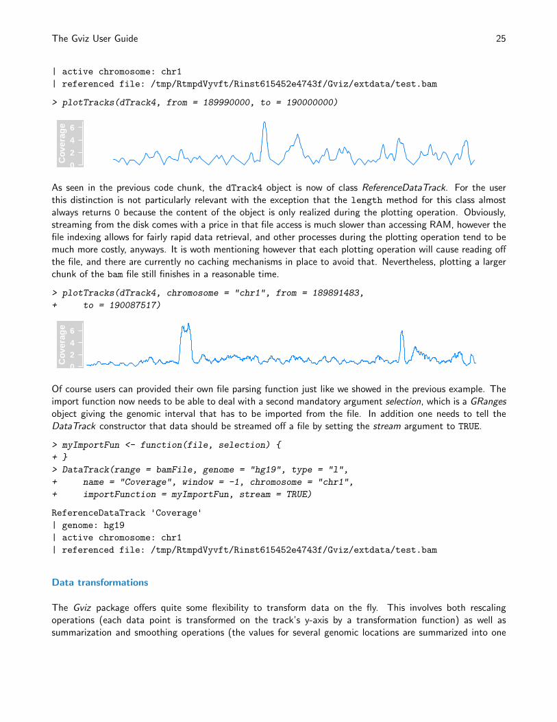
> plotTracks(dTrack4, from = 189990000, to = 190000000)
0
2
4
6
Cov
erag
e
As seen in the previous code chunk, the dTrack4 object is now of class ReferenceDataTrack. For the userthis distinction is not particularly relevant with the exception that the length method for this class almostalways returns 0 because the content of the object is only realized during the plotting operation. Obviously,streaming from the disk comes with a price in that file access is much slower than accessing RAM, however thefile indexing allows for fairly rapid data retrieval, and other processes during the plotting operation tend to bemuch more costly, anyways. It is woth mentioning however that each plotting operation will cause reading offthe file, and there are currently no caching mechanisms in place to avoid that. Nevertheless, plotting a largerchunk of the bam file still finishes in a reasonable time.
> plotTracks(dTrack4, chromosome = "chr1", from = 189891483,
+ to = 190087517)
0
2
4
6
Cov
erag
e
Of course users can provided their own file parsing function just like we showed in the previous example. Theimport function now needs to be able to deal with a second mandatory argument selection, which is a GRangesobject giving the genomic interval that has to be imported from the file. In addition one needs to tell theDataTrack constructor that data should be streamed off a file by setting the stream argument to TRUE.
> myImportFun <- function(file, selection) {
+ }
> DataTrack(range = bamFile, genome = "hg19", type = "l",
+ name = "Coverage", window = -1, chromosome = "chr1",
+ importFunction = myImportFun, stream = TRUE)
ReferenceDataTrack 'Coverage'
| genome: hg19
| active chromosome: chr1
| referenced file: /tmp/RtmpdVyvft/Rinst615452e4743f/Gviz/extdata/test.bam
Data transformations
The Gviz package offers quite some flexibility to transform data on the fly. This involves both rescalingoperations (each data point is transformed on the track’s y-axis by a transformation function) as well assummarization and smoothing operations (the values for several genomic locations are summarized into one
The Gviz User Guide 26
derived value on the track’s x-axis). To illustrate this let’s create a significantly bigger DataTrack than theone we used before, containing purely syntetic data for only a single sample.
> dat <- sin(seq(pi, 10 * pi, len = 500))
> dTrack.big <- DataTrack(start = seq(1, 100000, len = 500),
+ width = 15, chromosome = "chrX", genome = "hg19",
+ name = "sinus", data = sin(seq(pi, 5 * pi, len = 500)) *
+ runif(500, 0.5, 1.5))
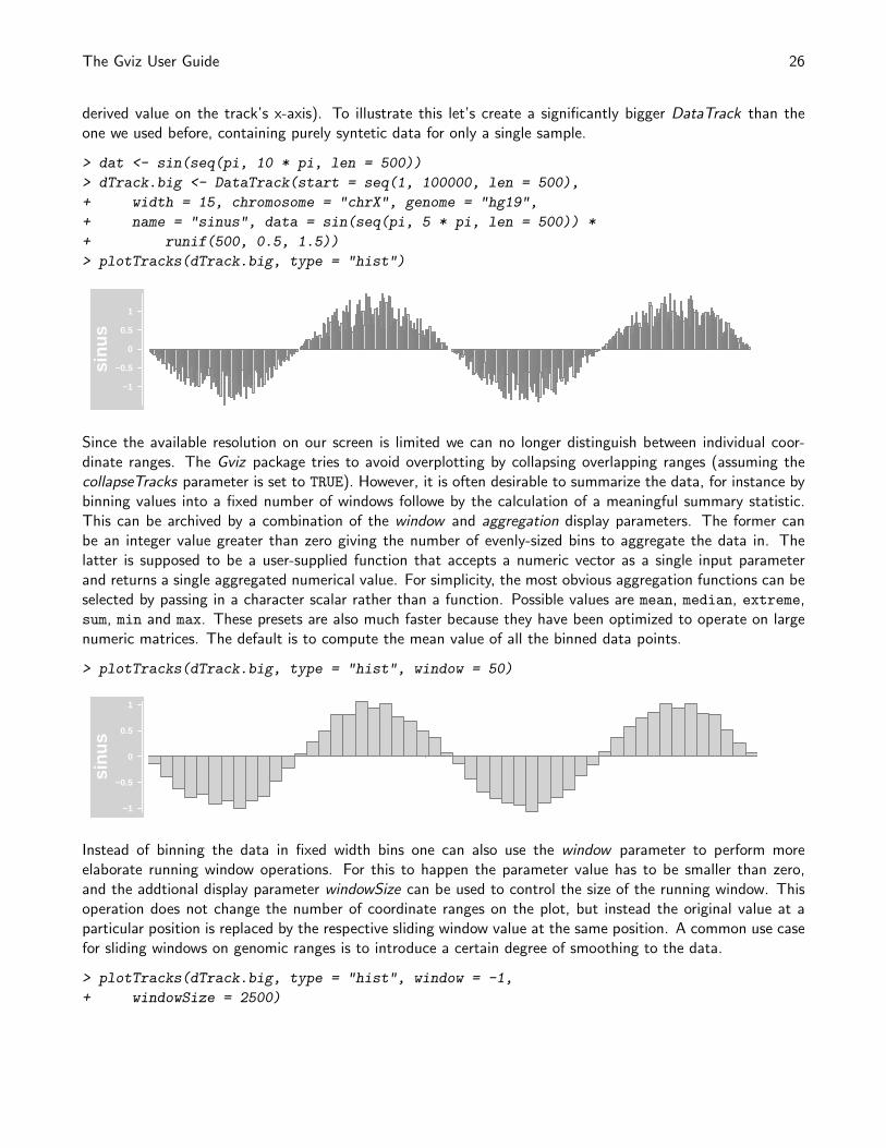
> plotTracks(dTrack.big, type = "hist")
−1
−0.5
0
0.5
1
sinu
s
Since the available resolution on our screen is limited we can no longer distinguish between individual coor-dinate ranges. The Gviz package tries to avoid overplotting by collapsing overlapping ranges (assuming thecollapseTracks parameter is set to TRUE). However, it is often desirable to summarize the data, for instance bybinning values into a fixed number of windows followe by the calculation of a meaningful summary statistic.This can be archived by a combination of the window and aggregation display parameters. The former canbe an integer value greater than zero giving the number of evenly-sized bins to aggregate the data in. Thelatter is supposed to be a user-supplied function that accepts a numeric vector as a single input parameterand returns a single aggregated numerical value. For simplicity, the most obvious aggregation functions can beselected by passing in a character scalar rather than a function. Possible values are mean, median, extreme,sum, min and max. These presets are also much faster because they have been optimized to operate on largenumeric matrices. The default is to compute the mean value of all the binned data points.
> plotTracks(dTrack.big, type = "hist", window = 50)
−1
−0.5
0
0.5
1
sinu
s
Instead of binning the data in fixed width bins one can also use the window parameter to perform moreelaborate running window operations. For this to happen the parameter value has to be smaller than zero,and the addtional display parameter windowSize can be used to control the size of the running window. Thisoperation does not change the number of coordinate ranges on the plot, but instead the original value at aparticular position is replaced by the respective sliding window value at the same position. A common use casefor sliding windows on genomic ranges is to introduce a certain degree of smoothing to the data.
> plotTracks(dTrack.big, type = "hist", window = -1,
+ windowSize = 2500)
The Gviz User Guide 27
−0.05
0
0.05
sinu
s
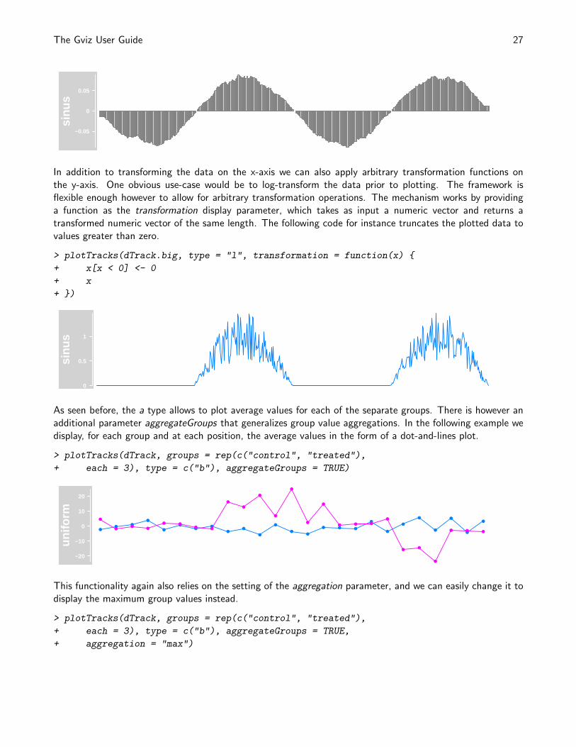
In addition to transforming the data on the x-axis we can also apply arbitrary transformation functions onthe y-axis. One obvious use-case would be to log-transform the data prior to plotting. The framework isflexible enough however to allow for arbitrary transformation operations. The mechanism works by providinga function as the transformation display parameter, which takes as input a numeric vector and returns atransformed numeric vector of the same length. The following code for instance truncates the plotted data tovalues greater than zero.
> plotTracks(dTrack.big, type = "l", transformation = function(x) {
+ x[x < 0] <- 0
+ x
+ })
0
0.5
1
sinu
s
As seen before, the a type allows to plot average values for each of the separate groups. There is however anadditional parameter aggregateGroups that generalizes group value aggregations. In the following example wedisplay, for each group and at each position, the average values in the form of a dot-and-lines plot.
> plotTracks(dTrack, groups = rep(c("control", "treated"),
+ each = 3), type = c("b"), aggregateGroups = TRUE)
−20
−10
0
10
20
unifo
rm
●●
●
●
●
●●
●
●●
●
●
●●
● ● ●
●
●
●
●
●
●
●
●●
●●
●
● ●● ●
●
●
●
●
●
●
●
● ● ●
●
●●
●
● ● ●
This functionality again also relies on the setting of the aggregation parameter, and we can easily change it todisplay the maximum group values instead.
> plotTracks(dTrack, groups = rep(c("control", "treated"),
+ each = 3), type = c("b"), aggregateGroups = TRUE,
+ aggregation = "max")
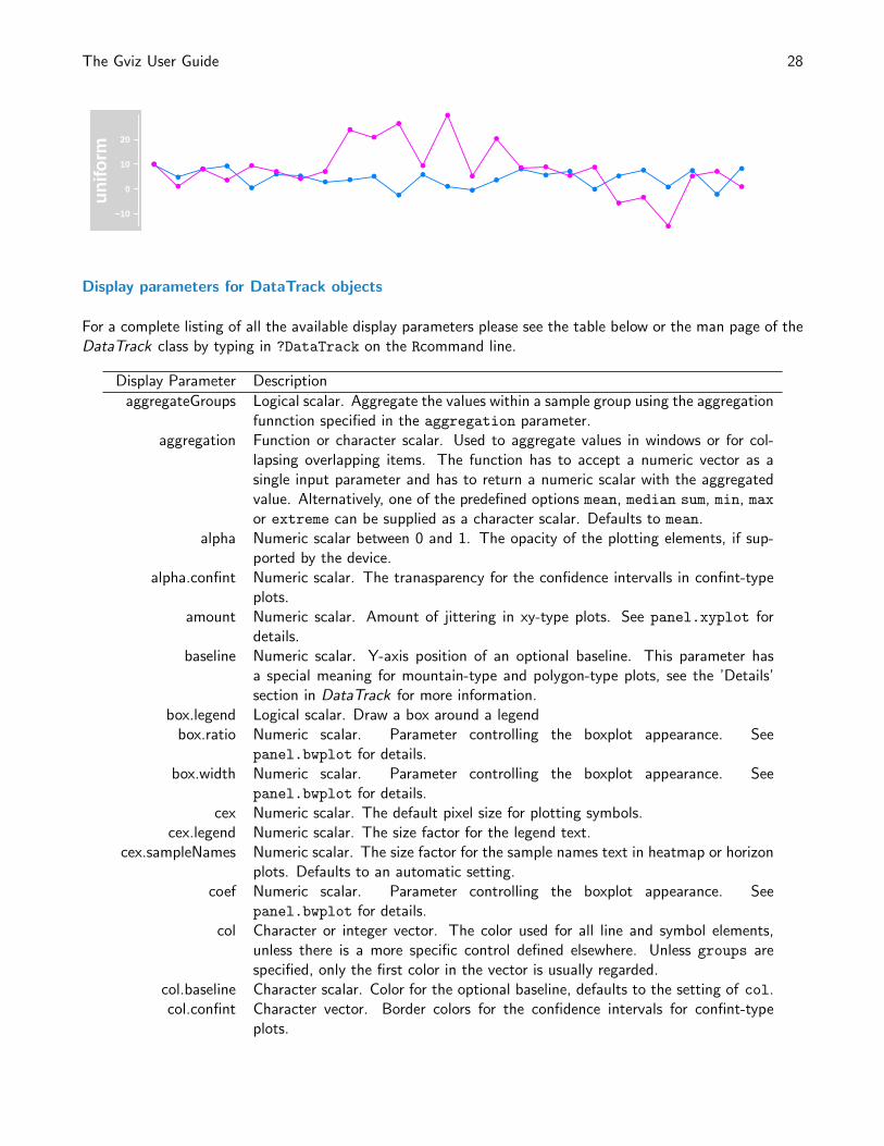
The Gviz User Guide 28
−10
0
10
20
unifo
rm ●
●
●●
●
● ●
● ●●
●
●
●●
●
●
●●
●
●●
●
●
●
●●
●
●
●
●●
●
●
●
●
●
●
●
●
●
● ●
●
●
●●
●
●●
●
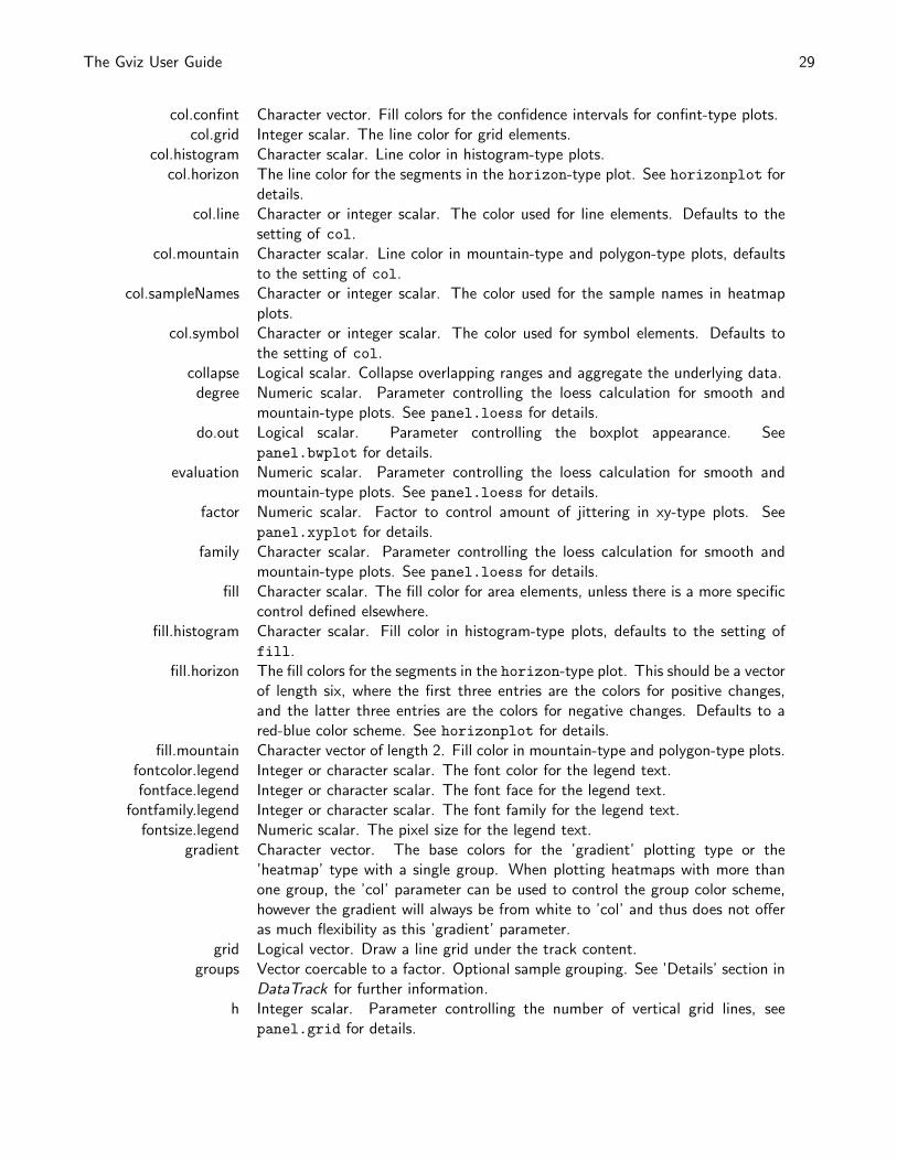
Display parameters for DataTrack objects
For a complete listing of all the available display parameters please see the table below or the man page of theDataTrack class by typing in ?DataTrack on the Rcommand line.
Display Parameter Description
aggregateGroups Logical scalar. Aggregate the values within a sample group using the aggregationfunnction specified in the aggregation parameter.
aggregation Function or character scalar. Used to aggregate values in windows or for col-lapsing overlapping items. The function has to accept a numeric vector as asingle input parameter and has to return a numeric scalar with the aggregatedvalue. Alternatively, one of the predefined options mean, median sum, min, maxor extreme can be supplied as a character scalar. Defaults to mean.
alpha Numeric scalar between 0 and 1. The opacity of the plotting elements, if sup-ported by the device.
alpha.confint Numeric scalar. The tranasparency for the confidence intervalls in confint-typeplots.
amount Numeric scalar. Amount of jittering in xy-type plots. See panel.xyplot fordetails.
baseline Numeric scalar. Y-axis position of an optional baseline. This parameter hasa special meaning for mountain-type and polygon-type plots, see the ’Details’section in DataTrack for more information.
box.legend Logical scalar. Draw a box around a legendbox.ratio Numeric scalar. Parameter controlling the boxplot appearance. See
panel.bwplot for details.box.width Numeric scalar. Parameter controlling the boxplot appearance. See
panel.bwplot for details.cex Numeric scalar. The default pixel size for plotting symbols.
cex.legend Numeric scalar. The size factor for the legend text.cex.sampleNames Numeric scalar. The size factor for the sample names text in heatmap or horizon
plots. Defaults to an automatic setting.coef Numeric scalar. Parameter controlling the boxplot appearance. See
panel.bwplot for details.col Character or integer vector. The color used for all line and symbol elements,
unless there is a more specific control defined elsewhere. Unless groups arespecified, only the first color in the vector is usually regarded.
col.baseline Character scalar. Color for the optional baseline, defaults to the setting of col.col.confint Character vector. Border colors for the confidence intervals for confint-type
plots.
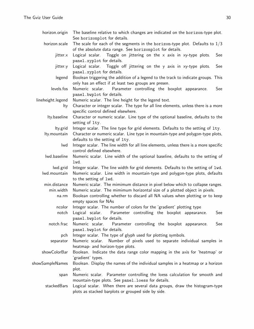
The Gviz User Guide 29
col.confint Character vector. Fill colors for the confidence intervals for confint-type plots.col.grid Integer scalar. The line color for grid elements.
col.histogram Character scalar. Line color in histogram-type plots.col.horizon The line color for the segments in the horizon-type plot. See horizonplot for
details.col.line Character or integer scalar. The color used for line elements. Defaults to the
setting of col.col.mountain Character scalar. Line color in mountain-type and polygon-type plots, defaults
to the setting of col.col.sampleNames Character or integer scalar. The color used for the sample names in heatmap
plots.col.symbol Character or integer scalar. The color used for symbol elements. Defaults to
the setting of col.collapse Logical scalar. Collapse overlapping ranges and aggregate the underlying data.
degree Numeric scalar. Parameter controlling the loess calculation for smooth andmountain-type plots. See panel.loess for details.
do.out Logical scalar. Parameter controlling the boxplot appearance. Seepanel.bwplot for details.
evaluation Numeric scalar. Parameter controlling the loess calculation for smooth andmountain-type plots. See panel.loess for details.
factor Numeric scalar. Factor to control amount of jittering in xy-type plots. Seepanel.xyplot for details.
family Character scalar. Parameter controlling the loess calculation for smooth andmountain-type plots. See panel.loess for details.
fill Character scalar. The fill color for area elements, unless there is a more specificcontrol defined elsewhere.
fill.histogram Character scalar. Fill color in histogram-type plots, defaults to the setting offill.
fill.horizon The fill colors for the segments in the horizon-type plot. This should be a vectorof length six, where the first three entries are the colors for positive changes,and the latter three entries are the colors for negative changes. Defaults to ared-blue color scheme. See horizonplot for details.
fill.mountain Character vector of length 2. Fill color in mountain-type and polygon-type plots.fontcolor.legend Integer or character scalar. The font color for the legend text.fontface.legend Integer or character scalar. The font face for the legend text.
fontfamily.legend Integer or character scalar. The font family for the legend text.fontsize.legend Numeric scalar. The pixel size for the legend text.
gradient Character vector. The base colors for the ’gradient’ plotting type or the’heatmap’ type with a single group. When plotting heatmaps with more thanone group, the ’col’ parameter can be used to control the group color scheme,however the gradient will always be from white to ’col’ and thus does not offeras much flexibility as this ’gradient’ parameter.
grid Logical vector. Draw a line grid under the track content.groups Vector coercable to a factor. Optional sample grouping. See ’Details’ section in
DataTrack for further information.h Integer scalar. Parameter controlling the number of vertical grid lines, see
panel.grid for details.
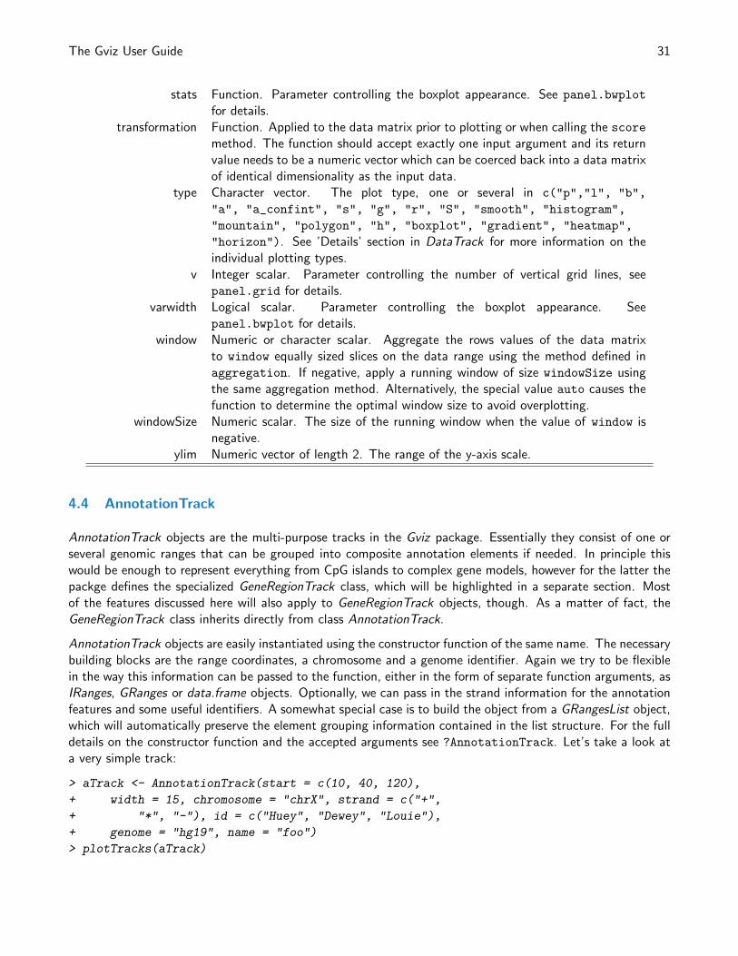
The Gviz User Guide 30
horizon.origin The baseline relative to which changes are indicated on the horizon-type plot.See horizonplot for details.
horizon.scale The scale for each of the segments in the horizon-type plot. Defaults to 1/3of the absolute data range. See horizonplot for details.
jitter.x Logical scalar. Toggle on jittering on the x axis in xy-type plots. Seepanel.xyplot for details.
jitter.y Logical scalar. Toggle off jittering on the y axis in xy-type plots. Seepanel.xyplot for details.
legend Boolean triggering the addition of a legend to the track to indicate groups. Thisonly has an effect if at least two groups are presen.
levels.fos Numeric scalar. Parameter controlling the boxplot appearance. Seepanel.bwplot for details.
lineheight.legend Numeric scalar. The line height for the legend text.lty Character or integer scalar. The type for all line elements, unless there is a more
specific control defined elsewhere.lty.baseline Character or numeric scalar. Line type of the optional baseline, defaults to the
setting of lty.lty.grid Integer scalar. The line type for grid elements. Defaults to the setting of lty.
lty.mountain Character or numeric scalar. Line type in mountain-type and polygon-type plots,defaults to the setting of lty.
lwd Integer scalar. The line width for all line elements, unless there is a more specificcontrol defined elsewhere.
lwd.baseline Numeric scalar. Line width of the optional baseline, defaults to the setting oflwd.
lwd.grid Integer scalar. The line width for grid elements. Defaults to the setting of lwd.lwd.mountain Numeric scalar. Line width in mountain-type and polygon-type plots, defaults
to the setting of lwd.min.distance Numeric scalar. The mimimum distance in pixel below which to collapse ranges.
min.width Numeric scalar. The mimimum horizontal size of a plotted object in pixels.na.rm Boolean controlling whether to discard all NA values when plotting or to keep
empty spaces for NAsncolor Integer scalar. The number of colors for the ’gradient’ plotting typenotch Logical scalar. Parameter controlling the boxplot appearance. See
panel.bwplot for details.notch.frac Numeric scalar. Parameter controlling the boxplot appearance. See
panel.bwplot for details.pch Integer scalar. The type of glyph used for plotting symbols.
separator Numeric scalar. Number of pixels used to separate individual samples inheatmap- and horizon-type plots.
showColorBar Boolean. Indicate the data range color mapping in the axis for ’heatmap’ or’gradient’ types.
showSampleNames Boolean. Display the names of the individual samples in a heatmap or a horizonplot.
span Numeric scalar. Parameter controlling the loess calculation for smooth andmountain-type plots. See panel.loess for details.
stackedBars Logical scalar. When there are several data groups, draw the histogram-typeplots as stacked barplots or grouped side by side.
The Gviz User Guide 31
stats Function. Parameter controlling the boxplot appearance. See panel.bwplot
for details.transformation Function. Applied to the data matrix prior to plotting or when calling the score
method. The function should accept exactly one input argument and its returnvalue needs to be a numeric vector which can be coerced back into a data matrixof identical dimensionality as the input data.
type Character vector. The plot type, one or several in c("p","l", "b",
"a", "a_confint", "s", "g", "r", "S", "smooth", "histogram",
"mountain", "polygon", "h", "boxplot", "gradient", "heatmap",
"horizon"). See ’Details’ section in DataTrack for more information on theindividual plotting types.
v Integer scalar. Parameter controlling the number of vertical grid lines, seepanel.grid for details.
varwidth Logical scalar. Parameter controlling the boxplot appearance. Seepanel.bwplot for details.
window Numeric or character scalar. Aggregate the rows values of the data matrixto window equally sized slices on the data range using the method defined inaggregation. If negative, apply a running window of size windowSize usingthe same aggregation method. Alternatively, the special value auto causes thefunction to determine the optimal window size to avoid overplotting.
windowSize Numeric scalar. The size of the running window when the value of window isnegative.
ylim Numeric vector of length 2. The range of the y-axis scale.
4.4 AnnotationTrack
AnnotationTrack objects are the multi-purpose tracks in the Gviz package. Essentially they consist of one orseveral genomic ranges that can be grouped into composite annotation elements if needed. In principle thiswould be enough to represent everything from CpG islands to complex gene models, however for the latter thepackge defines the specialized GeneRegionTrack class, which will be highlighted in a separate section. Mostof the features discussed here will also apply to GeneRegionTrack objects, though. As a matter of fact, theGeneRegionTrack class inherits directly from class AnnotationTrack.
AnnotationTrack objects are easily instantiated using the constructor function of the same name. The necessarybuilding blocks are the range coordinates, a chromosome and a genome identifier. Again we try to be flexiblein the way this information can be passed to the function, either in the form of separate function arguments, asIRanges, GRanges or data.frame objects. Optionally, we can pass in the strand information for the annotationfeatures and some useful identifiers. A somewhat special case is to build the object from a GRangesList object,which will automatically preserve the element grouping information contained in the list structure. For the fulldetails on the constructor function and the accepted arguments see ?AnnotationTrack. Let’s take a look ata very simple track:
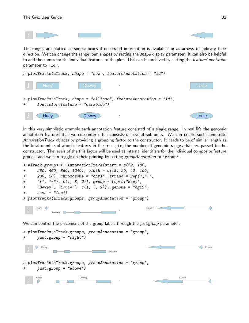
> aTrack <- AnnotationTrack(start = c(10, 40, 120),
+ width = 15, chromosome = "chrX", strand = c("+",
+ "*", "-"), id = c("Huey", "Dewey", "Louie"),
+ genome = "hg19", name = "foo")
> plotTracks(aTrack)
The Gviz User Guide 32
foo
The ranges are plotted as simple boxes if no strand information is available, or as arrows to indicate theirdirection. We can change the range item shapes by setting the shape display parameter. It can also be helpfulto add the names for the individual features to the plot. This can be archived by setting the featureAnnotationparameter to ’id’.
> plotTracks(aTrack, shape = "box", featureAnnotation = "id")
foo Huey Dewey Louie
> plotTracks(aTrack, shape = "ellipse", featureAnnotation = "id",
+ fontcolor.feature = "darkblue")
foo Huey Dewey Louie
In this very simplistic example each annotation feature consisted of a single range. In real life the genomicannotation features that we encounter often consists of several sub-units. We can create such compositeAnnotationTrack objects by providing a grouping factor to the constructor. It needs to be of similar length asthe total number of atomic features in the track, i.e, the number of genomic ranges that are passed to theconstructor. The levels of the this factor will be used as internal identifiers for the individual composite featuregroups, and we can toggle on their printing by setting groupAnnotation to ’group’.
> aTrack.groups <- AnnotationTrack(start = c(50, 180,
+ 260, 460, 860, 1240), width = c(15, 20, 40, 100,
+ 200, 20), chromosome = "chrX", strand = rep(c("+",
+ "*", "-"), c(1, 3, 2)), group = rep(c("Huey",
+ "Dewey", "Louie"), c(1, 3, 2)), genome = "hg19",
+ name = "foo")
> plotTracks(aTrack.groups, groupAnnotation = "group")
foo
Dewey
Huey Louie
We can control the placement of the group labels through the just.group parameter.
> plotTracks(aTrack.groups, groupAnnotation = "group",
+ just.group = "right")
foo
Dewey
Huey Louie
> plotTracks(aTrack.groups, groupAnnotation = "group",
+ just.group = "above")
foo DeweyHuey Louie
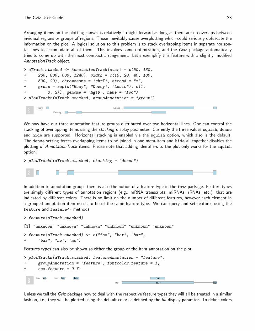
The Gviz User Guide 33
Arranging items on the plotting canvas is relatively straight forward as long as there are no overlaps betweeninvidiual regions or groups of regions. Those inevitably cause overplotting which could seriously obfuscate theinformation on the plot. A logical solution to this problem is to stack overlapping items in separate horizon-tal lines to accomodate all of them. This involves some optimization, and the Gviz package automaticallytries to come up with the most compact arrangement. Let’s exemplify this feature with a slightly modifiedAnnotationTrack object.
> aTrack.stacked <- AnnotationTrack(start = c(50, 180,
+ 260, 800, 600, 1240), width = c(15, 20, 40, 100,
+ 500, 20), chromosome = "chrX", strand = "*",
+ group = rep(c("Huey", "Dewey", "Louie"), c(1,
+ 3, 2)), genome = "hg19", name = "foo")
> plotTracks(aTrack.stacked, groupAnnotation = "group")
foo
Dewey
Huey Louie
We now have our three annotation feature groups distributed over two horizontal lines. One can control thestacking of overlapping items using the stacking display parameter. Currently the three values squish, denseand hide are supported. Horizontal stacking is enabled via the squish option, which also is the default.The dense setting forces overlapping items to be joined in one meta-item and hide all together disables theplotting of AnnotationTrack items. Please note that adding identifiers to the plot only works for the squish
option.
> plotTracks(aTrack.stacked, stacking = "dense")
foo
In addition to annotation groups there is also the notion of a feature type in the Gviz package. Feature typesare simply different types of annotation regions (e.g., mRNA transcripts, miRNAs, rRNAs, etc.) that areindicated by different colors. There is no limit on the number of different features, however each element ina grouped annotation item needs to be of the same feature type. We can query and set features using thefeature and feature<- methods.
> feature(aTrack.stacked)
[1] "unknown" "unknown" "unknown" "unknown" "unknown" "unknown"
> feature(aTrack.stacked) <- c("foo", "bar", "bar",
+ "bar", "no", "no")
Features types can also be shown as either the group or the item annotation on the plot.
> plotTracks(aTrack.stacked, featureAnnotation = "feature",
+ groupAnnotation = "feature", fontcolor.feature = 1,
+ cex.feature = 0.7)
foo foo bar bar bar
no no
barfoo
no
Unless we tell the Gviz package how to deal with the respective feature types they will all be treated in a similarfashion, i.e., they will be plotted using the default color as defined by the fill display paramter. To define colors
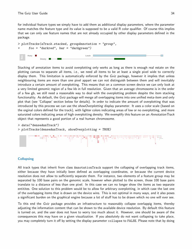
The Gviz User Guide 34
for individual feature types we simply have to add them as additional display parameters, where the parametername matches the feature type and its value is supposed to be a valid R color qualifier. Of course this impliesthat we can only use feature names that are not already occupied by other display parameters defined in thepackage.
> plotTracks(aTrack.stacked, groupAnnotation = "group",
+ foo = "darkred", bar = "darkgreen")
foo
Dewey
Huey Louie
Stacking of annotation items to avoid overplotting only works as long as there is enough real estate on theplotting canvas to separate all items, i.e., we need all items to be at least a single pixel wide to correctlydisplay them. This limitation is automatically enforced by the Gviz package, however it implies that unlessneighbouring items are more than one pixel appart we can not distinguish between them and will inevitablyintroduce a certain amount of overplotting. This means that on a common screen device we can only look ata very limited genomic region of a few kb in full resolution. Given that an average chromosome is in the orderof a few gb, we still need a reasonable way to deal with the overplotting problem despite the item stackingfunctionality. As default, the Gviz package will merge all overlapping items into one unified meta-item and onlyplot that (see ’Collapse’ section below for details). In order to indicate the amount of overplotting that wasintroduced by this process we can use the showOverplotting display parameter. It uses a color scale (based onthe orginal colors defined for the track), with lighter colors indicating areas of low or no overplotting, and moresaturated colors indicating areas of high overplotting density. We exemplify this feature on an AnnotationTrackobject that represents a good portion of a real human chromosome.
> data("denseAnnTrack")
> plotTracks(denseAnnTrack, showOverplotting = TRUE)
Collapsing
All track types that inherit from class AnnotationTrack support the collapsing of overlapping track items,either because they have initially been defined as overlapping coordinates, or because the current deviceresolution does not allow to sufficiently separate them. For instance, two elements of a feature group may beseparated by 100 base pairs on the genomic scale, however when plotted to the screen, those 100 base pairstranslate to a distance of less than one pixel. In this case we can no longer show the items as two separateentitites. One solution to this problem would be to allow for arbitrary overplotting, in which case the last oneof the overlapping items that is drawn on the device wins. This is not optimal in many ways, and it also posesa significant burden on the graphical engine because a lot of stuff has to be drawn which no one will ever see.
To this end the Gviz package provides an infrastructure to reasonably collapse overlappig items, therebyadjusting the information content that can be shown to the available device resolution. By default this featureis turned on, and the user does not have to worry too much about it. However, one should be aware of theconsequences this may have on a given visualization. If you absolutely do not want collapsing to take place,you may completely turn it off by setting the display parameter collapse to FALSE. Please note that by doing
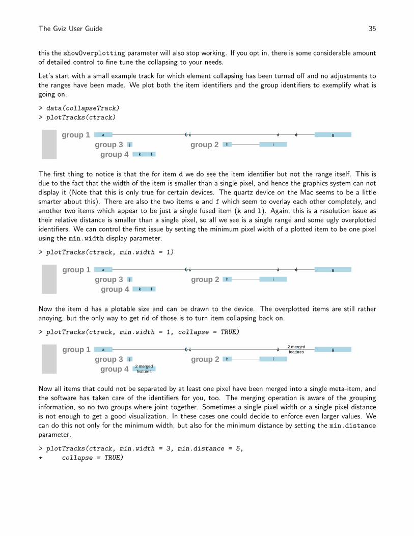
The Gviz User Guide 35
this the showOverplotting parameter will also stop working. If you opt in, there is some considerable amountof detailed control to fine tune the collapsing to your needs.
Let’s start with a small example track for which element collapsing has been turned off and no adjustments tothe ranges have been made. We plot both the item identifiers and the group identifiers to exemplify what isgoing on.
> data(collapseTrack)
> plotTracks(ctrack)
a b c d ef g
h ij
k l
group 1group 2group 3
group 4
The first thing to notice is that the for item d we do see the item identifier but not the range itself. This isdue to the fact that the width of the item is smaller than a single pixel, and hence the graphics system can notdisplay it (Note that this is only true for certain devices. The quartz device on the Mac seems to be a littlesmarter about this). There are also the two items e and f which seem to overlay each other completely, andanother two items which appear to be just a single fused item (k and l). Again, this is a resolution issue astheir relative distance is smaller than a single pixel, so all we see is a single range and some ugly overplottedidentifiers. We can control the first issue by setting the minimum pixel width of a plotted item to be one pixelusing the min.width display parameter.
> plotTracks(ctrack, min.width = 1)
a b c d ef g
h ij
k l
group 1group 2group 3
group 4
Now the item d has a plotable size and can be drawn to the device. The overplotted items are still ratheranoying, but the only way to get rid of those is to turn item collapsing back on.
> plotTracks(ctrack, min.width = 1, collapse = TRUE)
a b c d g
h ij
2 mergedfeatures
2 mergedfeatures
group 1group 2group 3
group 4
Now all items that could not be separated by at least one pixel have been merged into a single meta-item, andthe software has taken care of the identifiers for you, too. The merging operation is aware of the groupinginformation, so no two groups where joint together. Sometimes a single pixel width or a single pixel distanceis not enough to get a good visualization. In these cases one could decide to enforce even larger values. Wecan do this not only for the minimum width, but also for the minimum distance by setting the min.distance
parameter.
> plotTracks(ctrack, min.width = 3, min.distance = 5,
+ collapse = TRUE)
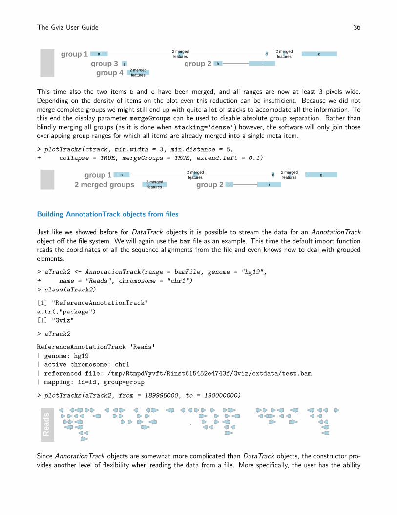
The Gviz User Guide 36
a d g
h ij
2 mergedfeatures
2 mergedfeatures
2 mergedfeatures
group 1group 2group 3
group 4
This time also the two items b and c have been merged, and all ranges are now at least 3 pixels wide.Depending on the density of items on the plot even this reduction can be insufficient. Because we did notmerge complete groups we might still end up with quite a lot of stacks to accomodate all the information. Tothis end the display parameter mergeGroups can be used to disable absolute group separation. Rather thanblindly merging all groups (as it is done when stacking=’dense’) however, the software will only join thoseoverlapping group ranges for which all items are already merged into a single meta item.
> plotTracks(ctrack, min.width = 3, min.distance = 5,
+ collapse = TRUE, mergeGroups = TRUE, extend.left = 0.1)
a d g
h i
2 mergedfeatures
2 mergedfeatures
3 mergedfeatures2 merged groups
group 1group 2
Building AnnotationTrack objects from files
Just like we showed before for DataTrack objects it is possible to stream the data for an AnnotationTrackobject off the file system. We will again use the bam file as an example. This time the default import functionreads the coordinates of all the sequence alignments from the file and even knows how to deal with groupedelements.
> aTrack2 <- AnnotationTrack(range = bamFile, genome = "hg19",
+ name = "Reads", chromosome = "chr1")
> class(aTrack2)
[1] "ReferenceAnnotationTrack"
attr(,"package")
[1] "Gviz"
> aTrack2
ReferenceAnnotationTrack 'Reads'
| genome: hg19
| active chromosome: chr1
| referenced file: /tmp/RtmpdVyvft/Rinst615452e4743f/Gviz/extdata/test.bam
| mapping: id=id, group=group
> plotTracks(aTrack2, from = 189995000, to = 190000000)
Rea
ds
Since AnnotationTrack objects are somewhat more complicated than DataTrack objects, the constructor pro-vides another level of flexibility when reading the data from a file. More specifically, the user has the ability
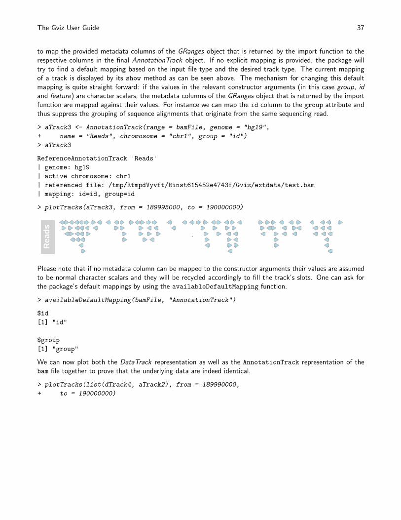
The Gviz User Guide 37
to map the provided metadata columns of the GRanges object that is returned by the import function to therespective columns in the final AnnotationTrack object. If no explicit mapping is provided, the package willtry to find a default mapping based on the input file type and the desired track type. The current mappingof a track is displayed by its show method as can be seen above. The mechanism for changing this defaultmapping is quite straight forward: if the values in the relevant constructor arguments (in this case group, idand feature) are character scalars, the metadata columns of the GRanges object that is returned by the importfunction are mapped against their values. For instance we can map the id column to the group attribute andthus suppress the grouping of sequence alignments that originate from the same sequencing read.
> aTrack3 <- AnnotationTrack(range = bamFile, genome = "hg19",
+ name = "Reads", chromosome = "chr1", group = "id")
> aTrack3
ReferenceAnnotationTrack 'Reads'
| genome: hg19
| active chromosome: chr1
| referenced file: /tmp/RtmpdVyvft/Rinst615452e4743f/Gviz/extdata/test.bam
| mapping: id=id, group=id
> plotTracks(aTrack3, from = 189995000, to = 190000000)
Rea
ds
Please note that if no metadata column can be mapped to the constructor arguments their values are assumedto be normal character scalars and they will be recycled accordingly to fill the track’s slots. One can ask forthe package’s default mappings by using the availableDefaultMapping function.
> availableDefaultMapping(bamFile, "AnnotationTrack")
$id
[1] "id"
$group
[1] "group"
We can now plot both the DataTrack representation as well as the AnnotationTrack representation of thebam file together to prove that the underlying data are indeed identical.
> plotTracks(list(dTrack4, aTrack2), from = 189990000,
+ to = 190000000)
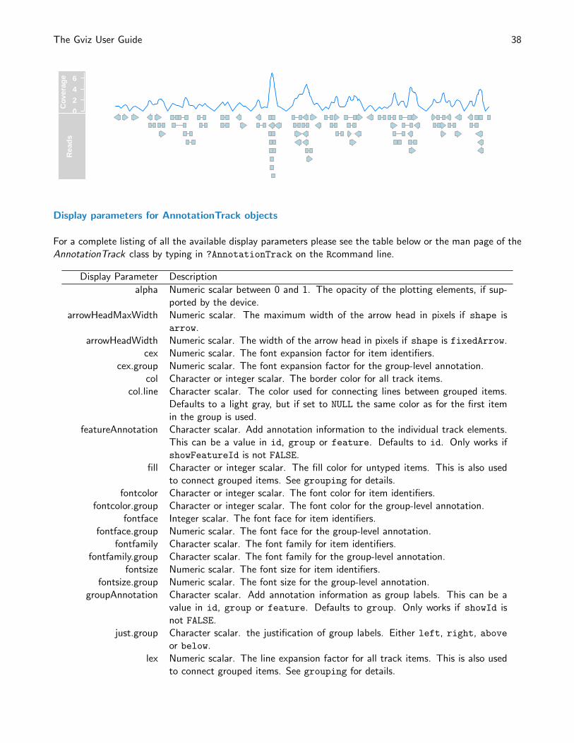
The Gviz User Guide 38
0246
Cov
erag
eR
eads
Display parameters for AnnotationTrack objects
For a complete listing of all the available display parameters please see the table below or the man page of theAnnotationTrack class by typing in ?AnnotationTrack on the Rcommand line.
Display Parameter Description
alpha Numeric scalar between 0 and 1. The opacity of the plotting elements, if sup-ported by the device.
arrowHeadMaxWidth Numeric scalar. The maximum width of the arrow head in pixels if shape isarrow.
arrowHeadWidth Numeric scalar. The width of the arrow head in pixels if shape is fixedArrow.cex Numeric scalar. The font expansion factor for item identifiers.
cex.group Numeric scalar. The font expansion factor for the group-level annotation.col Character or integer scalar. The border color for all track items.
col.line Character scalar. The color used for connecting lines between grouped items.Defaults to a light gray, but if set to NULL the same color as for the first itemin the group is used.
featureAnnotation Character scalar. Add annotation information to the individual track elements.This can be a value in id, group or feature. Defaults to id. Only works ifshowFeatureId is not FALSE.
fill Character or integer scalar. The fill color for untyped items. This is also usedto connect grouped items. See grouping for details.
fontcolor Character or integer scalar. The font color for item identifiers.fontcolor.group Character or integer scalar. The font color for the group-level annotation.
fontface Integer scalar. The font face for item identifiers.fontface.group Numeric scalar. The font face for the group-level annotation.
fontfamily Character scalar. The font family for item identifiers.fontfamily.group Character scalar. The font family for the group-level annotation.
fontsize Numeric scalar. The font size for item identifiers.fontsize.group Numeric scalar. The font size for the group-level annotation.
groupAnnotation Character scalar. Add annotation information as group labels. This can be avalue in id, group or feature. Defaults to group. Only works if showId isnot FALSE.
just.group Character scalar. the justification of group labels. Either left, right, aboveor below.
lex Numeric scalar. The line expansion factor for all track items. This is also usedto connect grouped items. See grouping for details.
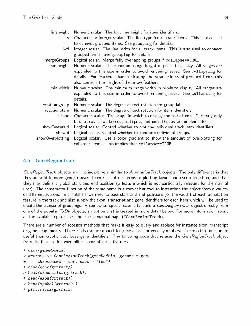
The Gviz User Guide 39
lineheight Numeric scalar. The font line height for item identifiers.lty Character or integer scalar. The line type for all track items. This is also used
to connect grouped items. See grouping for details.lwd Integer scalar. The line width for all track items. This is also used to connect
grouped items. See grouping for details.mergeGroups Logical scalar. Merge fully overlapping groups if collapse==TRUE.
min.height Numeric scalar. The minimum range height in pixels to display. All ranges areexpanded to this size in order to avoid rendering issues. See collapsing fordetails. For feathered bars indicating the strandedness of grouped items thisalso controls the height of the arrow feathers.
min.width Numeric scalar. The minimum range width in pixels to display. All ranges areexpanded to this size in order to avoid rendering issues. See collapsing fordetails.
rotation.group Numeric scalar. The degree of text rotation for group labels.rotation.item Numeric scalar. The degree of text rotation for item identifiers.
shape Character scalar. The shape in which to display the track items. Currently onlybox, arrow, fixedArrow, ellipse, and smallArrow are implemented.
showFeatureId Logical scalar. Control whether to plot the individual track item identifiers.showId Logical scalar. Control whether to annotate individual groups.
showOverplotting Logical scalar. Use a color gradient to show the amount of overplotting forcollapsed items. This implies that collapse==TRUE
4.5 GeneRegionTrack
GeneRegionTrack objects are in principle very similar to AnnotationTrack objects. The only difference is thatthey are a little more gene/transcript centric, both in terms of plotting layout and user interaction, and thatthey may define a global start and end position (a feature which is not particularly relevant for the normaluser). The constructor function of the same name is a convenient tool to instantiate the object from a varietyof different sources. In a nutshell, we need to pass start and end positions (or the width) of each annotationfeature in the track and also supply the exon, transcript and gene identifiers for each item which will be used tocreate the transcript groupings. A somewhat special case is to build a GeneRegionTrack object directly fromone of the popular TxDb objects, an option that is treated in more detail below. For more information aboutall the available options see the class’s manual page (?GeneRegionTrack).
There are a number of accessor methods that make it easy to query and replace for instance exon, transcriptor gene assignments. There is also some support for gene aliases or gene symbols which are often times moreuseful than cryptic data base gene identifiers. The following code that re-uses the GeneRegionTrack objectfrom the first section exemplifies some of these features.
> data(geneModels)
> grtrack <- GeneRegionTrack(geneModels, genome = gen,
+ chromosome = chr, name = "foo")
> head(gene(grtrack))
> head(transcript(grtrack))
> head(exon(grtrack))
> head(symbol(grtrack))
> plotTracks(grtrack)
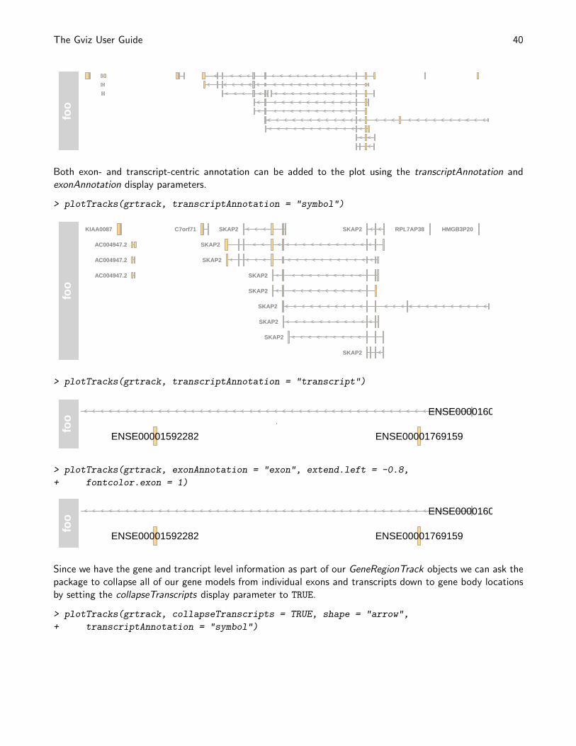
The Gviz User Guide 40
foo
Both exon- and transcript-centric annotation can be added to the plot using the transcriptAnnotation andexonAnnotation display parameters.
> plotTracks(grtrack, transcriptAnnotation = "symbol")
foo
KIAA0087
SKAP2
C7orf71 HMGB3P20
AC004947.2
AC004947.2
SKAP2
RPL7AP38
AC004947.2
SKAP2
SKAP2
SKAP2
SKAP2
SKAP2
SKAP2
SKAP2
SKAP2
> plotTracks(grtrack, transcriptAnnotation = "transcript")
foo
ENSE00001592282
ENSE00001609754
ENSE00001769159
ENSE00001686825
> plotTracks(grtrack, exonAnnotation = "exon", extend.left = -0.8,
+ fontcolor.exon = 1)
foo
ENSE00001592282
ENSE00001609754
ENSE00001769159
ENSE00001686825
Since we have the gene and trancript level information as part of our GeneRegionTrack objects we can ask thepackage to collapse all of our gene models from individual exons and transcripts down to gene body locationsby setting the collapseTranscripts display parameter to TRUE.
> plotTracks(grtrack, collapseTranscripts = TRUE, shape = "arrow",
+ transcriptAnnotation = "symbol")
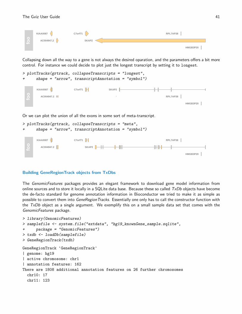
The Gviz User Guide 41
foo SKAP2
KIAA0087 RPL7AP38C7orf71
HMGB3P20
AC004947.2
Collapsing down all the way to a gene is not always the desired oparation, and the parameters offers a bit morecontrol. For instance we could decide to plot just the longest transcript by setting it to longest.
> plotTracks(grtrack, collapseTranscripts = "longest",
+ shape = "arrow", transcriptAnnotation = "symbol")
foo
KIAA0087 C7orf71
HMGB3P20
AC004947.2
SKAP2
RPL7AP38
Or we can plot the union of all the exons in some sort of meta-transcript.
> plotTracks(grtrack, collapseTranscripts = "meta",
+ shape = "arrow", transcriptAnnotation = "symbol")
foo SKAP2
KIAA0087 RPL7AP38C7orf71
HMGB3P20
AC004947.2
Building GeneRegionTrack objects from TxDbs
The GenomicFeatures packages provides an elegant framework to download gene model information fromonline sources and to store it locally in a SQLite data base. Because these so called TxDb objects have becomethe de-facto standard for genome annotation information in Bioconductor we tried to make it as simple aspossible to convert them into GeneRegionTracks. Essentially one only has to call the constructor function withthe TxDb object as a single argument. We exemplify this on a small sample data set that comes with theGenomicFeatures package.
> library(GenomicFeatures)
> samplefile <- system.file("extdata", "hg19_knownGene_sample.sqlite",
+ package = "GenomicFeatures")
> txdb <- loadDb(samplefile)
> GeneRegionTrack(txdb)
GeneRegionTrack 'GeneRegionTrack'
| genome: hg19
| active chromosome: chr1
| annotation features: 162
There are 1808 additional annotation features on 26 further chromosomes
chr10: 17
chr11: 123
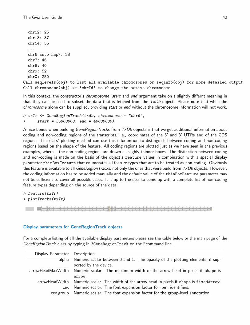
The Gviz User Guide 42
chr12: 25
chr13: 37
chr14: 55
...
chr6_ssto_hap7: 28
chr7: 46
chr8: 40
chr9: 52
chrX: 250
Call seqlevels(obj) to list all available chromosomes or seqinfo(obj) for more detailed output
Call chromosome(obj) <- 'chrId' to change the active chromosome
In this context, the constructor’s chromosome, start and end argument take on a slightly differnt meaning inthat they can be used to subset the data that is fetched from the TxDb object. Please note that while thechromosome alone can be supplied, providing start or end without the chromosome information will not work.
> txTr <- GeneRegionTrack(txdb, chromosome = "chr6",
+ start = 35000000, end = 40000000)
A nice bonus when building GeneRegionTracks from TxDb objects is that we get additional information aboutcoding and non-coding regions of the transcripts, i.e., coordinates of the 5’ and 3’ UTRs and of the CDSregions. The class’ plotting method can use this inforamtion to distinguish between coding and non-codingregions based on the shape of the feature. All coding regions are plotted just as we have seen in the previousexamples, whereas the non-coding regions are drawn as slighly thinner boxes. The distinction between codingand non-coding is made on the basis of the object’s feature values in combination with a special displayparameter thinBoxFeature that enumerates all feature types that are to be treated as non-coding. Obviouslythis feature is available to all GeneRegionTracks, not only the ones that were build from TxDb objects. However,the coding information has to be added manually and the default value of the thinBoxFeature parameter maynot be sufficient to cover all possible cases. It is up to the user to come up with a complete list of non-codingfeature types depending on the source of the data.
> feature(txTr)
> plotTracks(txTr)
Display parameters for GeneRegionTrack objects
For a complete listing of all the available display parameters please see the table below or the man page of theGeneRegionTrack class by typing in ?GeneRegionTrack on the Rcommand line.
Display Parameter Description
alpha Numeric scalar between 0 and 1. The opacity of the plotting elements, if sup-ported by the device.
arrowHeadMaxWidth Numeric scalar. The maximum width of the arrow head in pixels if shape isarrow.
arrowHeadWidth Numeric scalar. The width of the arrow head in pixels if shape is fixedArrow.cex Numeric scalar. The font expansion factor for item identifiers.
cex.group Numeric scalar. The font expansion factor for the group-level annotation.
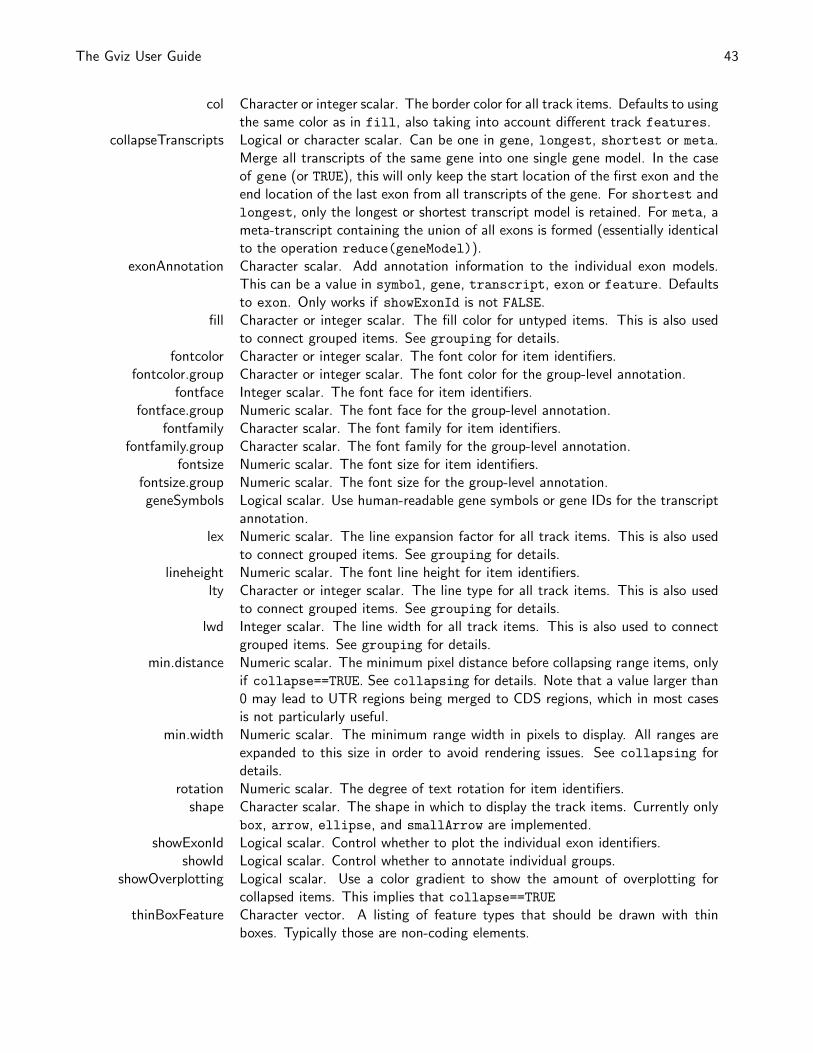
The Gviz User Guide 43
col Character or integer scalar. The border color for all track items. Defaults to usingthe same color as in fill, also taking into account different track features.
collapseTranscripts Logical or character scalar. Can be one in gene, longest, shortest or meta.Merge all transcripts of the same gene into one single gene model. In the caseof gene (or TRUE), this will only keep the start location of the first exon and theend location of the last exon from all transcripts of the gene. For shortest andlongest, only the longest or shortest transcript model is retained. For meta, ameta-transcript containing the union of all exons is formed (essentially identicalto the operation reduce(geneModel)).
exonAnnotation Character scalar. Add annotation information to the individual exon models.This can be a value in symbol, gene, transcript, exon or feature. Defaultsto exon. Only works if showExonId is not FALSE.
fill Character or integer scalar. The fill color for untyped items. This is also usedto connect grouped items. See grouping for details.
fontcolor Character or integer scalar. The font color for item identifiers.fontcolor.group Character or integer scalar. The font color for the group-level annotation.
fontface Integer scalar. The font face for item identifiers.fontface.group Numeric scalar. The font face for the group-level annotation.
fontfamily Character scalar. The font family for item identifiers.fontfamily.group Character scalar. The font family for the group-level annotation.
fontsize Numeric scalar. The font size for item identifiers.fontsize.group Numeric scalar. The font size for the group-level annotation.geneSymbols Logical scalar. Use human-readable gene symbols or gene IDs for the transcript
annotation.lex Numeric scalar. The line expansion factor for all track items. This is also used
to connect grouped items. See grouping for details.lineheight Numeric scalar. The font line height for item identifiers.
lty Character or integer scalar. The line type for all track items. This is also usedto connect grouped items. See grouping for details.
lwd Integer scalar. The line width for all track items. This is also used to connectgrouped items. See grouping for details.
min.distance Numeric scalar. The minimum pixel distance before collapsing range items, onlyif collapse==TRUE. See collapsing for details. Note that a value larger than0 may lead to UTR regions being merged to CDS regions, which in most casesis not particularly useful.
min.width Numeric scalar. The minimum range width in pixels to display. All ranges areexpanded to this size in order to avoid rendering issues. See collapsing fordetails.
rotation Numeric scalar. The degree of text rotation for item identifiers.shape Character scalar. The shape in which to display the track items. Currently only
box, arrow, ellipse, and smallArrow are implemented.showExonId Logical scalar. Control whether to plot the individual exon identifiers.
showId Logical scalar. Control whether to annotate individual groups.showOverplotting Logical scalar. Use a color gradient to show the amount of overplotting for
collapsed items. This implies that collapse==TRUEthinBoxFeature Character vector. A listing of feature types that should be drawn with thin
boxes. Typically those are non-coding elements.
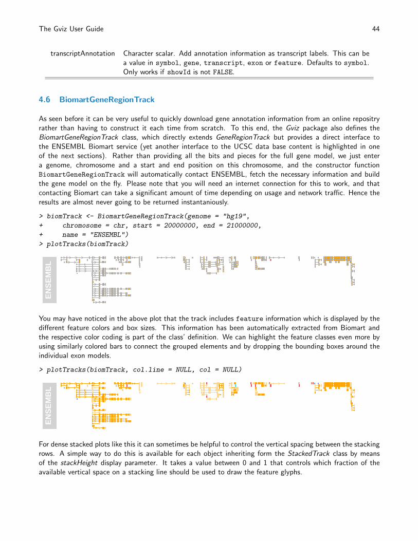
The Gviz User Guide 44
transcriptAnnotation Character scalar. Add annotation information as transcript labels. This can bea value in symbol, gene, transcript, exon or feature. Defaults to symbol.Only works if showId is not FALSE.
4.6 BiomartGeneRegionTrack
As seen before it can be very useful to quickly download gene annotation information from an online repositryrather than having to construct it each time from scratch. To this end, the Gviz package also defines theBiomartGeneRegionTrack class, which directly extends GeneRegionTrack but provides a direct interface tothe ENSEMBL Biomart service (yet another interface to the UCSC data base content is highlighted in oneof the next sections). Rather than providing all the bits and pieces for the full gene model, we just entera genome, chromosome and a start and end position on this chromosome, and the constructor functionBiomartGeneRegionTrack will automatically contact ENSEMBL, fetch the necessary information and buildthe gene model on the fly. Please note that you will need an internet connection for this to work, and thatcontacting Biomart can take a significant amount of time depending on usage and network traffic. Hence theresults are almost never going to be returned instantaniously.
> biomTrack <- BiomartGeneRegionTrack(genome = "hg19",
+ chromosome = chr, start = 20000000, end = 21000000,
+ name = "ENSEMBL")
> plotTracks(biomTrack)
EN
SE
MB
L
You may have noticed in the above plot that the track includes feature information which is displayed by thedifferent feature colors and box sizes. This information has been automatically extracted from Biomart andthe respective color coding is part of the class’ definition. We can highlight the feature classes even more byusing similarly colored bars to connect the grouped elements and by dropping the bounding boxes around theindividual exon models.
> plotTracks(biomTrack, col.line = NULL, col = NULL)
EN
SE
MB
L
For dense stacked plots like this it can sometimes be helpful to control the vertical spacing between the stackingrows. A simple way to do this is available for each object inheriting form the StackedTrack class by meansof the stackHeight display parameter. It takes a value between 0 and 1 that controls which fraction of theavailable vertical space on a stacking line should be used to draw the feature glyphs.
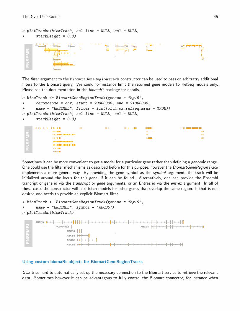
The Gviz User Guide 45
> plotTracks(biomTrack, col.line = NULL, col = NULL,
+ stackHeight = 0.3)
EN
SE
MB
L
The filter argument to the BiomartGeneRegionTrack constructor can be used to pass on arbitratry additionalfilters to the Biomart query. We could for instance limit the returned gene models to RefSeq models only.Please see the documentation in the biomaRt package for details.
> biomTrack <- BiomartGeneRegionTrack(genome = "hg19",
+ chromosome = chr, start = 20000000, end = 21000000,
+ name = "ENSEMBL", filter = list(with_ox_refseq_mrna = TRUE))
> plotTracks(biomTrack, col.line = NULL, col = NULL,
+ stackHeight = 0.3)
EN
SE
MB
L
Sometimes it can be more convenient to get a model for a particular gene rather than defining a genomic range.One could use the filter mechanisms as described before for this purpose, however the BiomartGeneRegionTrackimplements a more generic way. By providing the gene symbol as the symbol argument, the track will beinitialized around the locus for this gene, if it can be found. Alternatively, one can provide the Ensembltrancript or gene id via the transcript or gene arguments, or an Entrez id via the entrez argument. In all ofthese cases the constructor will also fetch models for other genes that overlap the same region. If that is notdesired one needs to provide an explicit Biomart filter.
> biomTrack <- BiomartGeneRegionTrack(genome = "hg19",
+ name = "ENSEMBL", symbol = "ABCB5")
> plotTracks(biomTrack)
EN
SE
MB
L
ABCB5
ABCB5
ABCB5
AC002486.3 ABCB5
ABCB5
ABCB5
Using custom biomaRt objects for BiomartGeneRegionTracks
Gviz tries hard to automatically set up the necessary connection to the Biomart service to retrieve the relevantdata. Sometimes however it can be advantagous to fully control the Biomart connector, for instance when
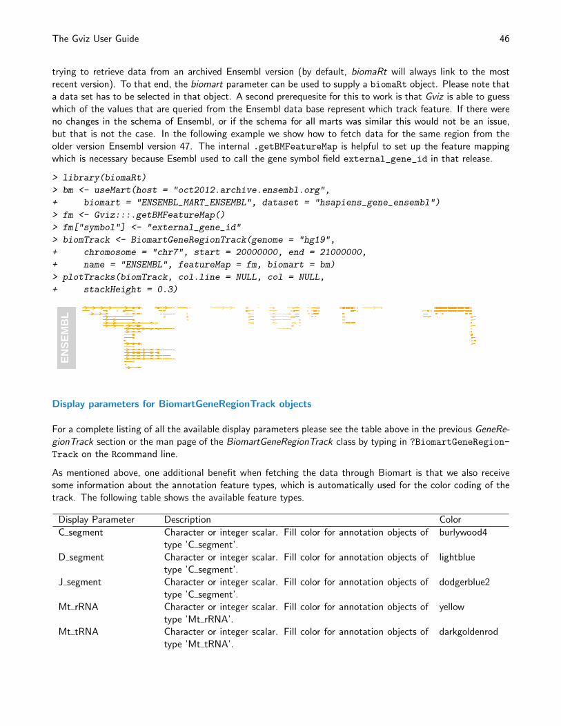
The Gviz User Guide 46
trying to retrieve data from an archived Ensembl version (by default, biomaRt will always link to the mostrecent version). To that end, the biomart parameter can be used to supply a biomaRt object. Please note thata data set has to be selected in that object. A second prerequesite for this to work is that Gviz is able to guesswhich of the values that are queried from the Ensembl data base represent which track feature. If there wereno changes in the schema of Ensembl, or if the schema for all marts was similar this would not be an issue,but that is not the case. In the following example we show how to fetch data for the same region from theolder version Ensembl version 47. The internal .getBMFeatureMap is helpful to set up the feature mappingwhich is necessary because Esembl used to call the gene symbol field external_gene_id in that release.
> library(biomaRt)
> bm <- useMart(host = "oct2012.archive.ensembl.org",
+ biomart = "ENSEMBL_MART_ENSEMBL", dataset = "hsapiens_gene_ensembl")
> fm <- Gviz:::.getBMFeatureMap()
> fm["symbol"] <- "external_gene_id"
> biomTrack <- BiomartGeneRegionTrack(genome = "hg19",
+ chromosome = "chr7", start = 20000000, end = 21000000,
+ name = "ENSEMBL", featureMap = fm, biomart = bm)
> plotTracks(biomTrack, col.line = NULL, col = NULL,
+ stackHeight = 0.3)
EN
SE
MB
L
Display parameters for BiomartGeneRegionTrack objects
For a complete listing of all the available display parameters please see the table above in the previous GeneRe-gionTrack section or the man page of the BiomartGeneRegionTrack class by typing in ?BiomartGeneRegion-
Track on the Rcommand line.
As mentioned above, one additional benefit when fetching the data through Biomart is that we also receivesome information about the annotation feature types, which is automatically used for the color coding of thetrack. The following table shows the available feature types.
Display Parameter Description Color
C segment Character or integer scalar. Fill color for annotation objects oftype ’C segment’.
burlywood4
D segment Character or integer scalar. Fill color for annotation objects oftype ’C segment’.
lightblue
J segment Character or integer scalar. Fill color for annotation objects oftype ’C segment’.
dodgerblue2
Mt rRNA Character or integer scalar. Fill color for annotation objects oftype ’Mt rRNA’.
yellow
Mt tRNA Character or integer scalar. Fill color for annotation objects oftype ’Mt tRNA’.
darkgoldenrod
The Gviz User Guide 47
Mt tRNA pseudogene Character or integer scalar. Fill color for annotation objects oftype ’Mt tRNA pseudogene’.
darkgoldenrod1
V segment Character or integer scalar. Fill color for annotation objects oftype ’V segment’.
aquamarine
miRNA Character or integer scalar. Fill color for annotation objects oftype ’L segment’.
cornflowerblue
miRNA pseudogene Character or integer scalar. Fill color for annotation objects oftype ’miRNA pseudogene’.
cornsilk
misc RNA Character or integer scalar. Fill color for annotation objects oftype ’misc RNA’.
cornsilk3
misc RNA pseudogene Character or integer scalar. Fill color for annotation objects oftype ’misc RNA pseudogene’.
cornsilk4
protein coding Character or integer scalar. Fill color for annotation objects oftype ’protein coding’.
orange
pseudogene Character or integer scalar. Fill color for annotation objects oftype ’pseudogene’.
brown1
rRNA Character or integer scalar. Fill color for annotation objects oftype ’rRNA’.
darkolivegreen1
rRNA pseudogene Character or integer scalar. Fill color for annotation objects oftype ’rRNA pseudogene’.
darkolivegreen
retrotransposed Character or integer scalar. Fill color for annotation objects oftype ’retrotransposed’.
blueviolet
scRNA Character or integer scalar. Fill color for annotation objects oftype ’scRNA’.
gold4
scRNA pseudogene Character or integer scalar. Fill color for annotation objects oftype ’scRNA pseudogene’.
darkorange2
snRNA Character or integer scalar. Fill color for annotation objects oftype ’snRNA’.
coral
snRNA pseudogene Character or integer scalar. Fill color for annotation objects oftype ’snRNA pseudogene’.
coral3
snoRNA Character or integer scalar. Fill color for annotation objects oftype ’snoRNA’.
cyan
snoRNA pseudogene Character or integer scalar. Fill color for annotation objects oftype ’snoRNA pseudogene’.
cyan2
tRNA pseudogene Character or integer scalar. Fill color for annotation objects oftype ’tRNA pseudogene’.
antiquewhite3
verbose Logical scalar. Report data loading events from Bioamart orretrieval from cache.
FALSE
4.7 DetailsAnnotationTrack
It is sometimes desirable to add more detailed information to particular ranges in an Gviz plot for which thenotion of genomic coordinates no longer makes sense. For instance, the ranges in an AnnotationTrack mayrepresent probe locations on a genome, and for each of these probes a number of measurements from multiplesamples and from different sample groups are available. To this end, the DetailsAnnotationTrack provides aflexible interface to further annotate genomic regions with arbitrary additional information. This is archivedby splitting the AnnotationTrack plotting region into two horizontal sections: the lower section containing the
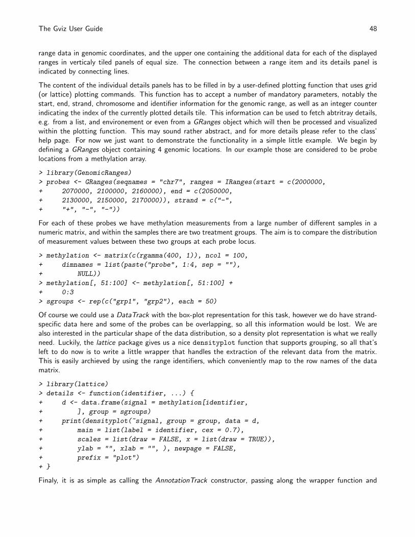
The Gviz User Guide 48
range data in genomic coordinates, and the upper one containing the additional data for each of the displayedranges in verticaly tiled panels of equal size. The connection between a range item and its details panel isindicated by connecting lines.
The content of the individual details panels has to be filled in by a user-defined plotting function that uses grid(or lattice) plotting commands. This function has to accept a number of mandatory parameters, notably thestart, end, strand, chromosome and identifier information for the genomic range, as well as an integer counterindicating the index of the currently plotted details tile. This information can be used to fetch abtritray details,e.g. from a list, and environement or even from a GRanges object which will then be processed and visualizedwithin the plotting function. This may sound rather abstract, and for more details please refer to the class’help page. For now we just want to demonstrate the functionality in a simple little example. We begin bydefining a GRanges object containing 4 genomic locations. In our example those are considered to be probelocations from a methylation array.
> library(GenomicRanges)
> probes <- GRanges(seqnames = "chr7", ranges = IRanges(start = c(2000000,
+ 2070000, 2100000, 2160000), end = c(2050000,
+ 2130000, 2150000, 2170000)), strand = c("-",
+ "+", "-", "-"))
For each of these probes we have methylation measurements from a large number of different samples in anumeric matrix, and within the samples there are two treatment groups. The aim is to compare the distributionof measurement values between these two groups at each probe locus.
> methylation <- matrix(c(rgamma(400, 1)), ncol = 100,
+ dimnames = list(paste("probe", 1:4, sep = ""),
+ NULL))
> methylation[, 51:100] <- methylation[, 51:100] +
+ 0:3
> sgroups <- rep(c("grp1", "grp2"), each = 50)
Of course we could use a DataTrack with the box-plot representation for this task, however we do have strand-specific data here and some of the probes can be overlapping, so all this information would be lost. We arealso interested in the particular shape of the data distribution, so a density plot representation is what we reallyneed. Luckily, the lattice package gives us a nice densityplot function that supports grouping, so all that’sleft to do now is to write a little wrapper that handles the extraction of the relevant data from the matrix.This is easily archieved by using the range identifiers, which conveniently map to the row names of the datamatrix.
> library(lattice)
> details <- function(identifier, ...) {
+ d <- data.frame(signal = methylation[identifier,
+ ], group = sgroups)
+ print(densityplot(~signal, group = group, data = d,
+ main = list(label = identifier, cex = 0.7),
+ scales = list(draw = FALSE, x = list(draw = TRUE)),
+ ylab = "", xlab = "", ), newpage = FALSE,
+ prefix = "plot")
+ }
Finaly, it is as simple as calling the AnnotationTrack constructor, passing along the wrapper function and
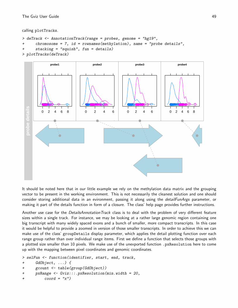
The Gviz User Guide 49
calling plotTracks.
> deTrack <- AnnotationTrack(range = probes, genome = "hg19",
+ chromosome = 7, id = rownames(methylation), name = "probe details",
+ stacking = "squish", fun = details)
> plotTracks(deTrack)
prob
e de
tails
probe1
0 2 4 6 8
● ●●● ●●●●●●● ●● ●●● ●●● ●●●●●● ●●● ●●● ●● ●● ●●●●●●● ●● ●● ●●●●●●● ● ●●●●●●●●●● ●● ●●●●● ●●● ●● ●● ●●● ●● ●●●●● ●●● ●●● ●● ●●●●
probe2
0 2 4 6
● ●●●● ●●●● ●● ●●● ●● ●●●● ●●● ●● ●● ●●● ●● ●● ●●●● ●●● ●●● ● ●● ●●● ●● ●●●● ●●● ●●●● ● ●● ●● ●● ●●●●●● ●● ●● ● ●● ●●● ●● ●● ●● ●● ●●● ●●●
probe3
0 2 4 6
● ● ●●●●● ●●●●●●● ● ●● ●● ●● ● ●● ●●●● ●● ●●●● ●●●●●● ●●●●● ●●● ●● ● ●●●● ●●●●●● ●●●● ● ●●●●●●●● ●●●●● ●●●●●●● ●●●● ●●●●● ●● ●● ●
probe4
0 2 4 6 8
●●●●● ●● ●● ●●●●●●●●●●● ●● ●●●●●●●● ●●●● ●●●●●● ●●● ●●● ●●●● ●●● ●●●● ●● ●● ● ●●● ●●●●● ●●●●●●●●●●●●● ●●●●●● ●●●● ●●●●● ●●
● ● ● ●
● ●
●
●
It should be noted here that in our little example we rely on the methylation data matrix and the groupingvector to be present in the working environment. This is not necessarily the cleanest solution and one shouldconsider storing additional data in an evironment, passing it along using the detailFunArgs parameter, ormaking it part of the details function in form of a closure. The class’ help page provides further instructions.
Another use case for the DetailsAnnotationTrack class is to deal with the problem of very different featuresizes within a single track. For instance, we may be looking at a rather large genomic region containing onebig transcript with many widely spaced exons and a bunch of smaller, more compact transcripts. In this caseit would be helpful to provide a zoomed in version of those smaller transcripts. In order to achieve this we canmake use of the class’ groupDetails display parameter, which applies the detail plotting function over eachrange group rather than over individual range items. First we define a function that selects those groups witha plotted size smaller than 10 pixels. We make use of the unexported function .pxResolution here to comeup with the mapping between pixel coordinates and genomic coordinates.
> selFun <- function(identifier, start, end, track,
+ GdObject, ...) {
+ gcount <- table(group(GdObject))
+ pxRange <- Gviz:::.pxResolution(min.width = 20,
+ coord = "x")
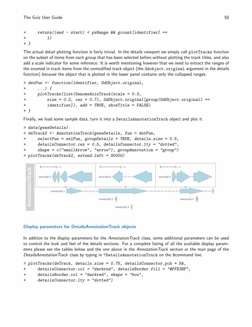
The Gviz User Guide 50
+ return((end - start) < pxRange && gcount[identifier] ==
+ 1)
+ }
The actual detail plotting function is fairly trivial. In the details viewport we simply call plotTracks functionon the subset of items from each group that has been selected before without plotting the track titles, and alsoadd a scale indicator for some reference. It is worth mentioning however that we need to extract the ranges ofthe zoomed in track items from the unmodified track object (the Gdobject.original argument in the detailsfunction) because the object that is plotted in the lower panel contains only the collapsed ranges.
> detFun <- function(identifier, GdObject.original,
+ ...) {
+ plotTracks(list(GenomeAxisTrack(scale = 0.3,
+ size = 0.2, cex = 0.7), GdObject.original[group(GdObject.original) ==
+ identifier]), add = TRUE, showTitle = FALSE)
+ }
Finally, we load some sample data, turn it into a DetailsAnnotationTrack object and plot it.
> data(geneDetails)
> deTrack2 <- AnnotationTrack(geneDetails, fun = detFun,
+ selectFun = selFun, groupDetails = TRUE, details.size = 0.5,
+ detailsConnector.cex = 0.5, detailsConnector.lty = "dotted",
+ shape = c("smallArrow", "arrow"), groupAnnotation = "group")
> plotTracks(deTrack2, extend.left = 90000)
Ann
otat
ionT
rack
4 kb
transcript 2
2 kb
transcript 3
5 kb
transcript 4
transcript 1
transcript 2
transcript 3
transcript 4
● ● ●
●
●
●
Display parameters for DetailsAnnotationTrack objects
In addtion to the display parameters for the AnnotationTrack class, some additional parameters can be usedto control the look and feel of the details sections. For a complete listing of all the available display param-eters please see the tables below and the one above in the AnnotationTrack section or the man page of theDetailsAnnotationTrack class by typing in ?DetailsAnnotationTrack on the Rcommand line.
> plotTracks(deTrack, details.size = 0.75, detailsConnector.pch = NA,
+ detailsConnector.col = "darkred", detailsBorder.fill = "#FFE3BF",
+ detailsBorder.col = "darkred", shape = "box",
+ detailsConnector.lty = "dotted")
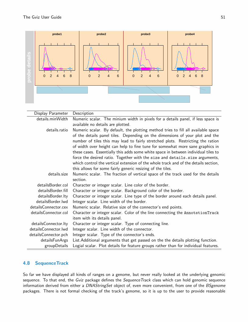
The Gviz User Guide 51
prob
e de
tails
probe1
0 2 4 6 8
● ●●● ●●●●●●● ●● ●●● ●●● ●●●●●● ●●● ●●● ●● ●● ●●●●●●● ●● ●● ●●●●●●● ● ●●●●●●●●●● ●● ●●●●● ●●● ●● ●● ●●● ●● ●●●●● ●●● ●●● ●● ●●●●
probe2
0 2 4 6
● ●●●● ●●●● ●● ●●● ●● ●●●● ●●● ●● ●● ●●● ●● ●● ●●●● ●●● ●●● ● ●● ●●● ●● ●●●● ●●● ●●●● ● ●● ●● ●● ●●●●●● ●● ●● ● ●● ●●● ●● ●● ●● ●● ●●● ●●●
probe3
0 2 4 6
● ● ●●●●● ●●●●●●● ● ●● ●● ●● ● ●● ●●●● ●● ●●●● ●●●●●● ●●●●● ●●● ●● ● ●●●● ●●●●●● ●●●● ● ●●●●●●●● ●●●●● ●●●●●●● ●●●● ●●●●● ●● ●● ●
probe4
0 2 4 6 8
●●●●● ●● ●● ●●●●●●●●●●● ●● ●●●●●●●● ●●●● ●●●●●● ●●● ●●● ●●●● ●●● ●●●● ●● ●● ● ●●● ●●●●● ●●●●●●●●●●●●● ●●●●●● ●●●● ●●●●● ●●
Display Parameter Description
details.minWidth Numeric scalar. The minium width in pixels for a details panel, if less space isavailable no details are plotted.
details.ratio Numeric scalar. By default, the plotting method tries to fill all available spaceof the details panel tiles. Depending on the dimensions of your plot and thenumber of tiles this may lead to fairly stretched plots. Restricting the rationof width over height can help to fine tune for somewhat more sane graphics inthese cases. Essentially this adds some white space in between individual tiles toforce the desired ratio. Together with the size and details.size arguments,which control the vertical extension of the whole track and of the details section,this allows for some fairly generic resizing of the tiles.
details.size Numeric scalar. The fraction of vertical space of the track used for the detailssection.
detailsBorder.col Character or integer scalar. Line color of the border.detailsBorder.fill Character or integer scalar. Background color of the border.detailsBorder.lty Character or integer scalar. Line type of the border around each details panel.
detailsBorder.lwd Integer scalar. Line width of the border.detailsConnector.cex Numeric scalar. Relative size of the connector’s end points.detailsConnector.col Character or integer scalar. Color of the line connecting the AnnotstionTrack
item with its details panel.detailsConnector.lty Character or integer scalar. Type of connecting line.
detailsConnector.lwd Integer scalar. Line width of the connector.detailsConnector.pch Integer scalar. Type of the connector’s ends.
detailsFunArgs List.Additional arguments that get passed on the the details plotting function.groupDetails Logial scalar. Plot details for feature groups rather than for individual features.
4.8 SequenceTrack
So far we have displayed all kinds of ranges on a genome, but never really looked at the underlying genomicsequence. To that end, the Gviz package defines the SequenceTrack class which can hold genomic sequenceinformation derived from either a DNAStringSet object of, even more convenient, from one of the BSgenomepackages. There is not formal checking of the track’s genome, so it is up to the user to provide reasonable
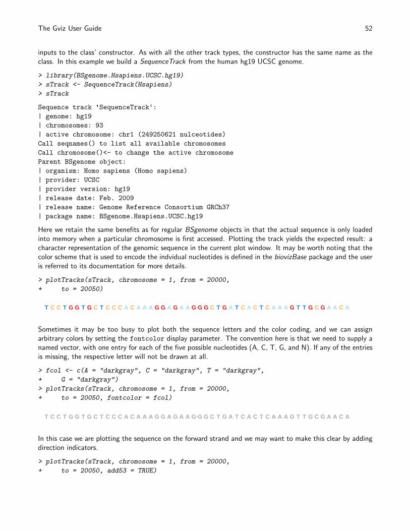
The Gviz User Guide 52
inputs to the class’ constructor. As with all the other track types, the constructor has the same name as theclass. In this example we build a SequenceTrack from the human hg19 UCSC genome.
> library(BSgenome.Hsapiens.UCSC.hg19)
> sTrack <- SequenceTrack(Hsapiens)
> sTrack
Sequence track 'SequenceTrack':
| genome: hg19
| chromosomes: 93
| active chromosome: chr1 (249250621 nulceotides)
Call seqnames() to list all available chromosomes
Call chromosome()<- to change the active chromosome
Parent BSgenome object:
| organism: Homo sapiens (Homo sapiens)
| provider: UCSC
| provider version: hg19
| release date: Feb. 2009
| release name: Genome Reference Consortium GRCh37
| package name: BSgenome.Hsapiens.UCSC.hg19
Here we retain the same benefits as for regular BSgenome objects in that the actual sequence is only loadedinto memory when a particular chromosome is first accessed. Plotting the track yields the expected result: acharacter representation of the genomic sequence in the current plot window. It may be worth noting that thecolor scheme that is used to encode the indvidual nucleotides is defined in the biovizBase package and the useris referred to its documentation for more details.
> plotTracks(sTrack, chromosome = 1, from = 20000,
+ to = 20050)
T C C T G G T G C T C C C A C A A A G G A G A A G G G C T G A T C A C T C A A A G T T G C G A A C A
Sometimes it may be too busy to plot both the sequence letters and the color coding, and we can assignarbitrary colors by setting the fontcolor display parameter. The convention here is that we need to supply anamed vector, with one entry for each of the five possible nucleotides (A, C, T, G, and N). If any of the entriesis missing, the respective letter will not be drawn at all.
> fcol <- c(A = "darkgray", C = "darkgray", T = "darkgray",
+ G = "darkgray")
> plotTracks(sTrack, chromosome = 1, from = 20000,
+ to = 20050, fontcolor = fcol)
T C C T G G T G C T C C C A C A A A G G A G A A G G G C T G A T C A C T C A A A G T T G C G A A C A
In this case we are plotting the sequence on the forward strand and we may want to make this clear by addingdirection indicators.
> plotTracks(sTrack, chromosome = 1, from = 20000,
+ to = 20050, add53 = TRUE)
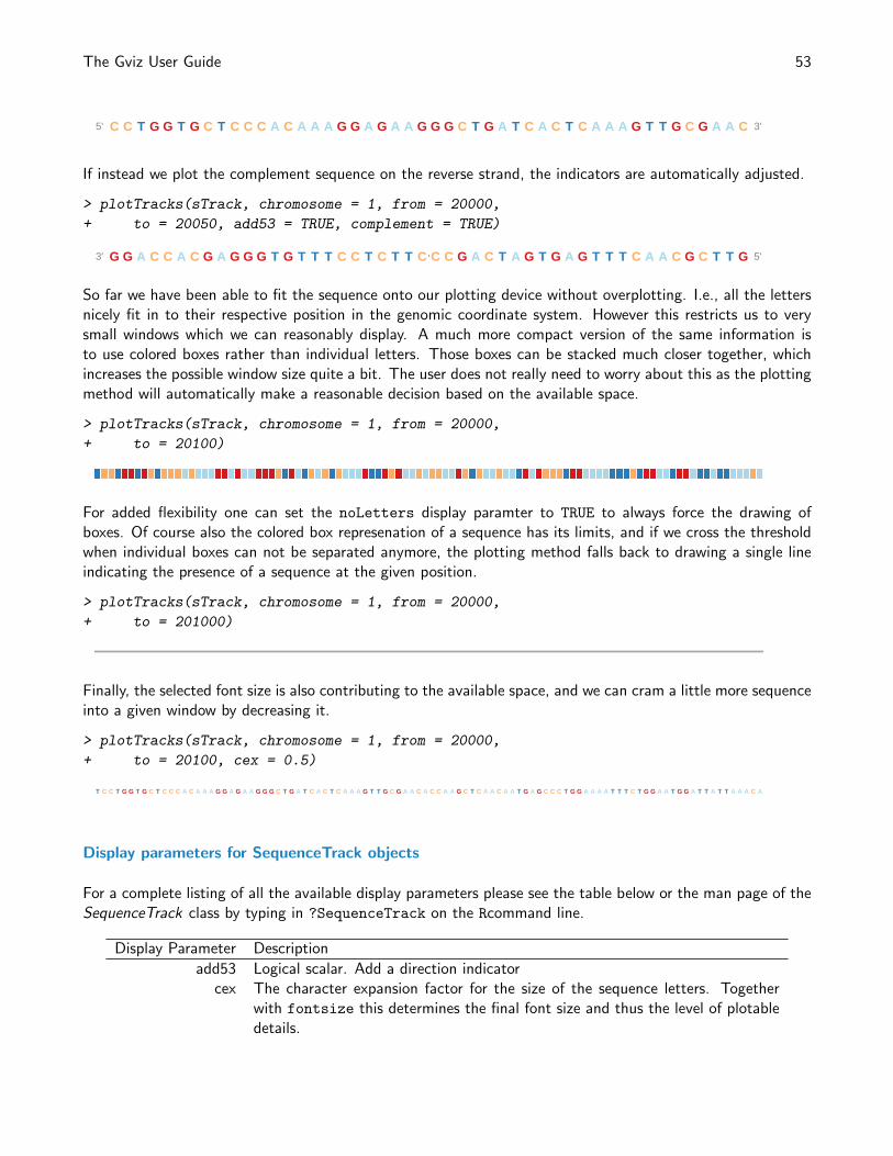
The Gviz User Guide 53
C C T G G T G C T C C C A C A A A G G A G A A G G G C T G A T C A C T C A A A G T T G C G A A C5' 3'
If instead we plot the complement sequence on the reverse strand, the indicators are automatically adjusted.
> plotTracks(sTrack, chromosome = 1, from = 20000,
+ to = 20050, add53 = TRUE, complement = TRUE)
G G A C C A C G A G G G T G T T T C C T C T T C C C G A C T A G T G A G T T T C A A C G C T T G3' 5'
So far we have been able to fit the sequence onto our plotting device without overplotting. I.e., all the lettersnicely fit in to their respective position in the genomic coordinate system. However this restricts us to verysmall windows which we can reasonably display. A much more compact version of the same information isto use colored boxes rather than individual letters. Those boxes can be stacked much closer together, whichincreases the possible window size quite a bit. The user does not really need to worry about this as the plottingmethod will automatically make a reasonable decision based on the available space.
> plotTracks(sTrack, chromosome = 1, from = 20000,
+ to = 20100)
For added flexibility one can set the noLetters display paramter to TRUE to always force the drawing ofboxes. Of course also the colored box represenation of a sequence has its limits, and if we cross the thresholdwhen individual boxes can not be separated anymore, the plotting method falls back to drawing a single lineindicating the presence of a sequence at the given position.
> plotTracks(sTrack, chromosome = 1, from = 20000,
+ to = 201000)
Finally, the selected font size is also contributing to the available space, and we can cram a little more sequenceinto a given window by decreasing it.
> plotTracks(sTrack, chromosome = 1, from = 20000,
+ to = 20100, cex = 0.5)
T C C T G G T G C T C C C A C A A A G G A G A A G G G C T G A T C A C T C A A A G T T G C G A A C A C C A A G C T C A A C A A T G A G C C C T G G A A A A T T T C T G G A A T G G A T T A T T A A A C A
Display parameters for SequenceTrack objects
For a complete listing of all the available display parameters please see the table below or the man page of theSequenceTrack class by typing in ?SequenceTrack on the Rcommand line.
Display Parameter Description
add53 Logical scalar. Add a direction indicatorcex The character expansion factor for the size of the sequence letters. Together
with fontsize this determines the final font size and thus the level of plotabledetails.
The Gviz User Guide 54
col Character scalar. The color of the line when no indiviual letters can be plotteddue to size limitations.
complement Logical scalar. Plot the sequence complement.fontcolor Character vector. The colors used for the 5 possible nucleotides (G, A, T, C,
N). Defaults to use colors as defined in the biovizBase package.fontface Numeric scalar. The face of the font.fontsize Numeric scalar. Controls the size of the sequence letters and thus also the level
of plotable details.lwd Numeric scalar. The width of the line when no indiviual letters can be plotted
due to size limitations.min.width Numeric scalar. The minimum width in pixels of the colored boxes that are
drawn when no indiviual letters can be plotted due to size limitations. If thehorizontal space that a single base occupies is smaller than this value, only ahorizontal line is drawn to indicate the presence of a sequence.
noLetters Logical scalar. Always plot colored boxes (or a line) regardles of the availablespace.
rotation Numeric scalar. The rotation angle for each individual letter in the sequence.
4.9 AlignmentsTrack
Plots of aligned sequences, typically from next generation sequencing experiments can be quite helpful, forinstance when visually inspecting the validity of a called SNP. Those alignments are usually stored in BAM files.As shown in some of the previous section we can deal with these files in a fairly crude way by coupling themto either an AnnotationTrack or a DataTrack. The utility of the generated plots however is fairly limited, andwe want in particular support for gapped and paired aligments, and show differences of the individual readsequences to a reference.
The AlignmentsTrack class is designed to help in exactly these tasks. In its typical manifestation it is alsoa member of the ReferenceTrack class, enabling memory efficient streaming directly off a file. Even thoughthis file does not necessarily have to be a BAM file, the automatic import will only work for those. For allother file representations of alignments a user will have to provide their own import function, and this topicis further discussed in the class’ documentation. For this demonstation let’s use a small BAM file for whichpaired NGS reads have been mapped to an extract of the human hg19 genome. The data originate from anRNASeq experiment, and the alignements have been performed using the STAR aligner allowing for gaps. Wealso download some gene annotation data for that region from Biomart.
Again, creating the AlignmentsTrack object is as simple as calling the constructor function of the same name.We set the isPaired argument to TRUE in order to tell the constructor that it should expect paired reads. Pleasenote that TRUE is the default value for this parameter and usually things will still work even if the reads donot originate from a paired end library. In other words, the default setting could be used as a poor-man’sautodetection, however it make more sense to supply the argument explicitely if you know what type of datato expect.
> afrom <- 2960000
> ato <- 3160000
> alTrack <- AlignmentsTrack(system.file(package = "Gviz",
+ "extdata", "gapped.bam"), isPaired = TRUE)
> bmt <- BiomartGeneRegionTrack(genome = "hg19", chromosome = "chr12",
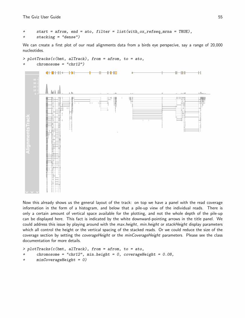
The Gviz User Guide 55
+ start = afrom, end = ato, filter = list(with_ox_refseq_mrna = TRUE),
+ stacking = "dense")
We can create a first plot of our read alignments data from a birds eye perspecive, say a range of 20,000nucleotides.
> plotTracks(c(bmt, alTrack), from = afrom, to = ato,
+ chromosome = "chr12")
010203040
Alig
nmen
tsTr
ack
Now this already shows us the general layout of the track: on top we have a panel with the read coverageinformation in the form of a histogram, and below that a pile-up view of the individual reads. There isonly a certain amount of vertical space available for the plotting, and not the whole depth of the pile-upcan be displayed here. This fact is indicated by the white downward-pointing arrows in the title panel. Wecould address this issue by playing around with the max.height, min.height or stackHeight display parameterswhich all control the height or the vertical spacing of the stacked reads. Or we could reduce the size of thecoverage section by setting the coverageHeight or the minCoverageHeight parameters. Please see the classdocumentation for more details.
> plotTracks(c(bmt, alTrack), from = afrom, to = ato,
+ chromosome = "chr12", min.height = 0, coverageHeight = 0.08,
+ minCoverageHeight = 0)
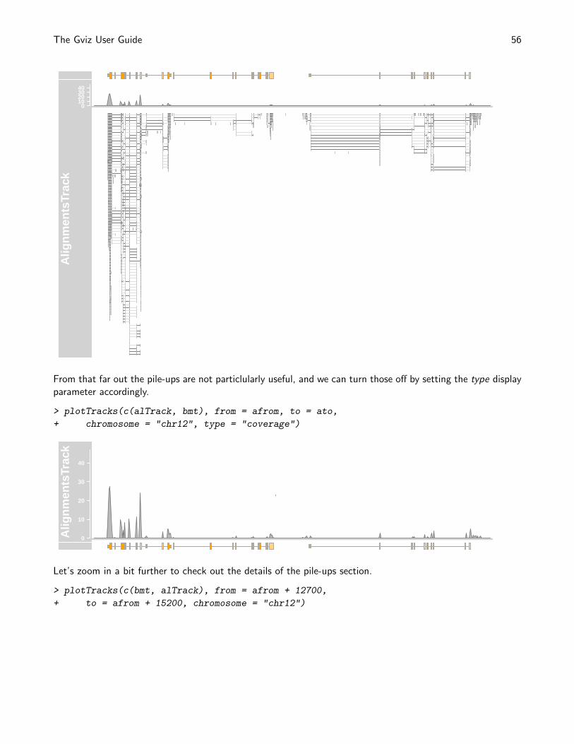
The Gviz User Guide 56
010203040
Alig
nmen
tsTr
ack
From that far out the pile-ups are not particlularly useful, and we can turn those off by setting the type displayparameter accordingly.
> plotTracks(c(alTrack, bmt), from = afrom, to = ato,
+ chromosome = "chr12", type = "coverage")
0
10
20
30
40
Alig
nmen
tsTr
ack
Let’s zoom in a bit further to check out the details of the pile-ups section.
> plotTracks(c(bmt, alTrack), from = afrom + 12700,
+ to = afrom + 15200, chromosome = "chr12")
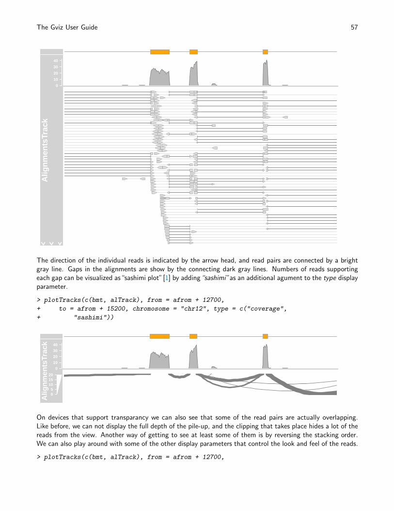
The Gviz User Guide 57
0
10
20
30
40
Alig
nmen
tsTr
ack
The direction of the individual reads is indicated by the arrow head, and read pairs are connected by a brightgray line. Gaps in the alignments are show by the connecting dark gray lines. Numbers of reads supportingeach gap can be visualized as“sashimi plot”[1] by adding“sashimi”as an additional agument to the type displayparameter.
> plotTracks(c(bmt, alTrack), from = afrom + 12700,
+ to = afrom + 15200, chromosome = "chr12", type = c("coverage",
+ "sashimi"))
0
10
20
30
40
05
101520
Alig
nmen
tsTr
ack
On devices that support transparancy we can also see that some of the read pairs are actually overlapping.Like before, we can not display the full depth of the pile-up, and the clipping that takes place hides a lot of thereads from the view. Another way of getting to see at least some of them is by reversing the stacking order.We can also play around with some of the other display parameters that control the look and feel of the reads.
> plotTracks(c(bmt, alTrack), from = afrom + 12700,
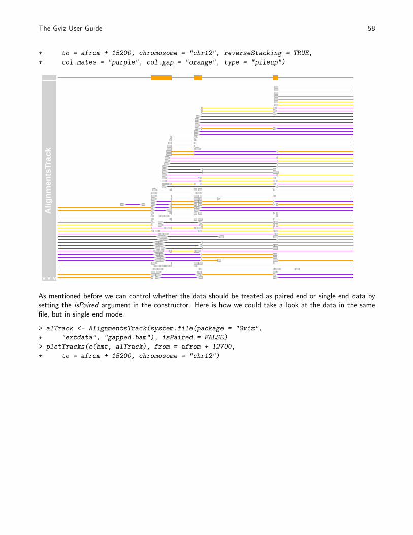
The Gviz User Guide 58
+ to = afrom + 15200, chromosome = "chr12", reverseStacking = TRUE,
+ col.mates = "purple", col.gap = "orange", type = "pileup")
Alig
nmen
tsTr
ack
As mentioned before we can control whether the data should be treated as paired end or single end data bysetting the isPaired argument in the constructor. Here is how we could take a look at the data in the samefile, but in single end mode.
> alTrack <- AlignmentsTrack(system.file(package = "Gviz",
+ "extdata", "gapped.bam"), isPaired = FALSE)
> plotTracks(c(bmt, alTrack), from = afrom + 12700,
+ to = afrom + 15200, chromosome = "chr12")
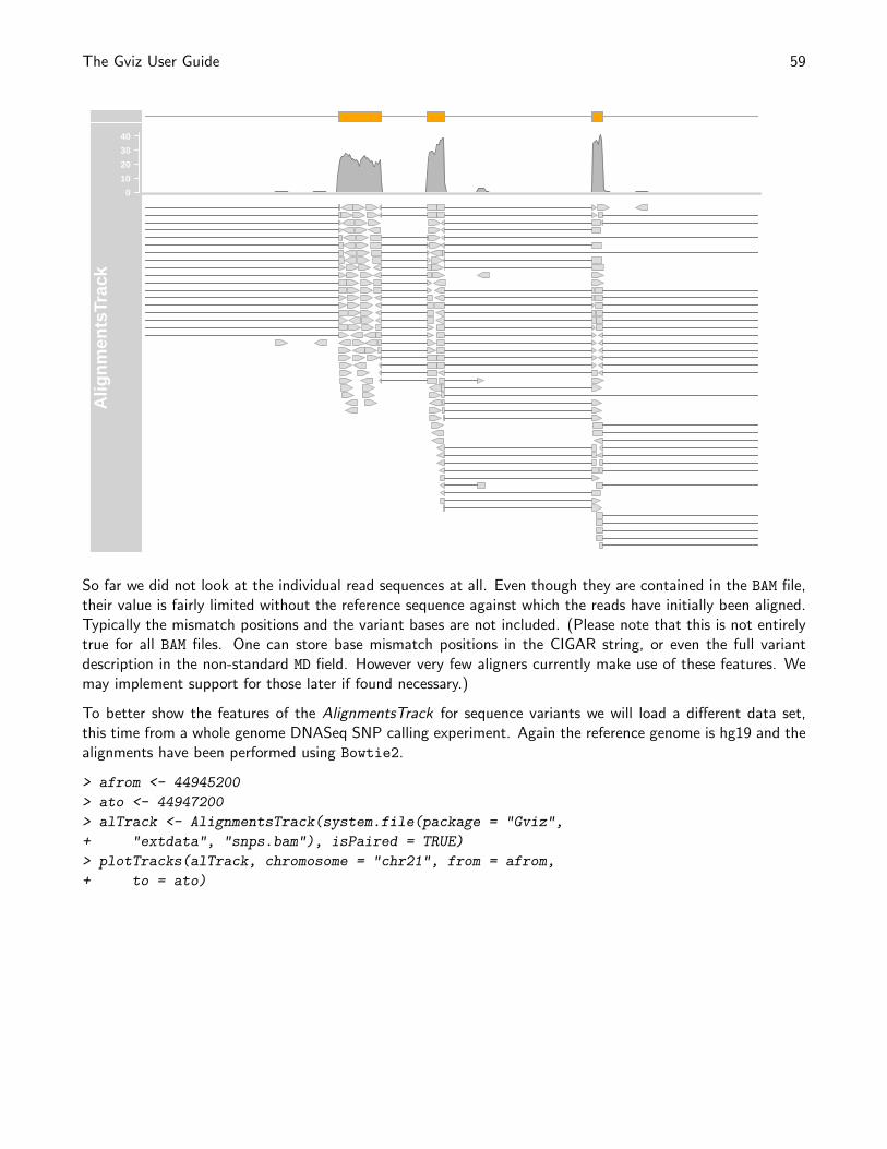
The Gviz User Guide 59
0
10
20
30
40
Alig
nmen
tsTr
ack
So far we did not look at the individual read sequences at all. Even though they are contained in the BAM file,their value is fairly limited without the reference sequence against which the reads have initially been aligned.Typically the mismatch positions and the variant bases are not included. (Please note that this is not entirelytrue for all BAM files. One can store base mismatch positions in the CIGAR string, or even the full variantdescription in the non-standard MD field. However very few aligners currently make use of these features. Wemay implement support for those later if found necessary.)
To better show the features of the AlignmentsTrack for sequence variants we will load a different data set,this time from a whole genome DNASeq SNP calling experiment. Again the reference genome is hg19 and thealignments have been performed using Bowtie2.
> afrom <- 44945200
> ato <- 44947200
> alTrack <- AlignmentsTrack(system.file(package = "Gviz",
+ "extdata", "snps.bam"), isPaired = TRUE)
> plotTracks(alTrack, chromosome = "chr21", from = afrom,
+ to = ato)
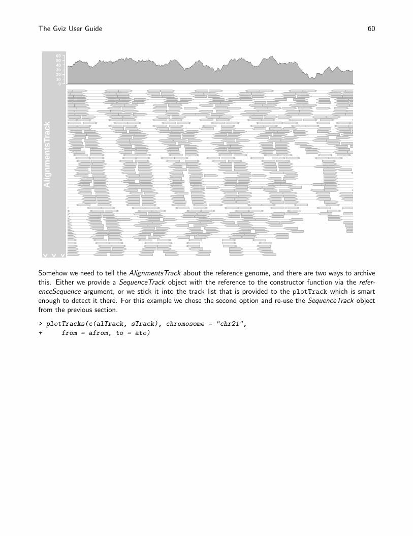
The Gviz User Guide 60
0102030405060
Alig
nmen
tsTr
ack
Somehow we need to tell the AlignmentsTrack about the reference genome, and there are two ways to archivethis. Either we provide a SequenceTrack object with the reference to the constructor function via the refer-enceSequence argument, or we stick it into the track list that is provided to the plotTrack which is smartenough to detect it there. For this example we chose the second option and re-use the SequenceTrack objectfrom the previous section.
> plotTracks(c(alTrack, sTrack), chromosome = "chr21",
+ from = afrom, to = ato)
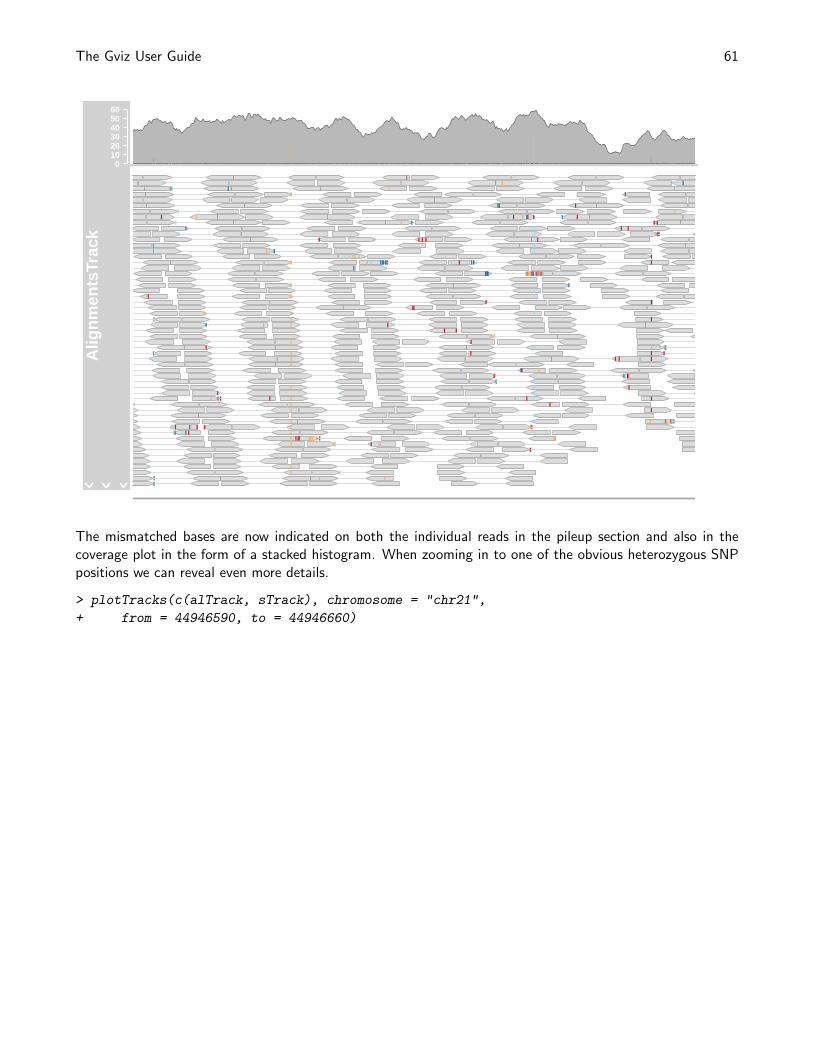
The Gviz User Guide 61
0102030405060
Alig
nmen
tsTr
ack
The mismatched bases are now indicated on both the individual reads in the pileup section and also in thecoverage plot in the form of a stacked histogram. When zooming in to one of the obvious heterozygous SNPpositions we can reveal even more details.
> plotTracks(c(alTrack, sTrack), chromosome = "chr21",
+ from = 44946590, to = 44946660)
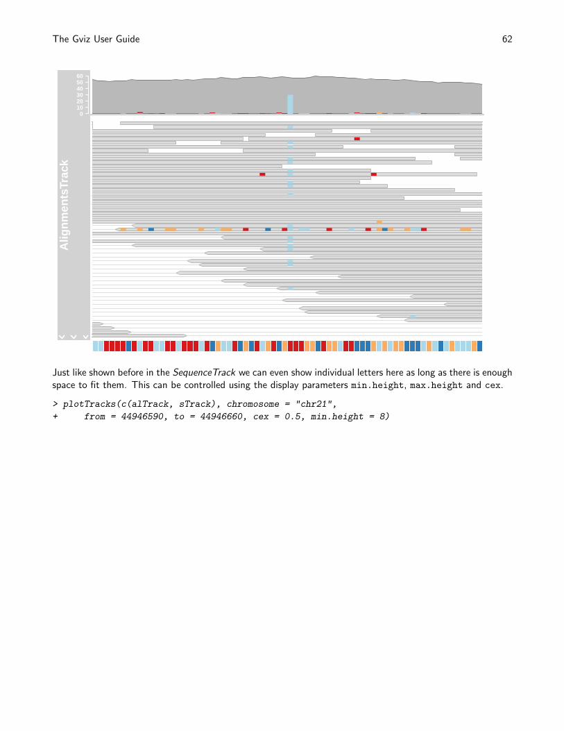
The Gviz User Guide 62
0102030405060
Alig
nmen
tsTr
ack
Just like shown before in the SequenceTrack we can even show individual letters here as long as there is enoughspace to fit them. This can be controlled using the display parameters min.height, max.height and cex.
> plotTracks(c(alTrack, sTrack), chromosome = "chr21",
+ from = 44946590, to = 44946660, cex = 0.5, min.height = 8)
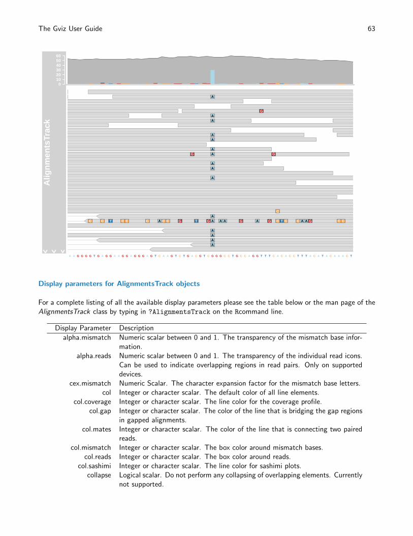
The Gviz User Guide 63
0102030405060
Alig
nmen
tsTr
ack
C C T C C C A C C G
G
T G
A
A
A
A
AA
A
A
A
A
A
A
A
AA
A
A
A A G A
G
G
G
C
C T C C A A G C C
A A G G G G T G A G G A A G G A G G G A G T C A A G T C T G A C G T C G G G C C T G C C A G G T T T C A C A C C T T T A C A T A C A A A C T
Display parameters for AlignmentsTrack objects
For a complete listing of all the available display parameters please see the table below or the man page of theAlignmentsTrack class by typing in ?AlignmentsTrack on the Rcommand line.
Display Parameter Description
alpha.mismatch Numeric scalar between 0 and 1. The transparency of the mismatch base infor-mation.
alpha.reads Numeric scalar between 0 and 1. The transparency of the individual read icons.Can be used to indicate overlapping regions in read pairs. Only on supporteddevices.
cex.mismatch Numeric Scalar. The character expansion factor for the mismatch base letters.col Integer or character scalar. The default color of all line elements.
col.coverage Integer or character scalar. The line color for the coverage profile.col.gap Integer or character scalar. The color of the line that is bridging the gap regions
in gapped alignments.col.mates Integer or character scalar. The color of the line that is connecting two paired
reads.col.mismatch Integer or character scalar. The box color around mismatch bases.
col.reads Integer or character scalar. The box color around reads.col.sashimi Integer or character scalar. The line color for sashimi plots.
collapse Logical scalar. Do not perform any collapsing of overlapping elements. Currentlynot supported.
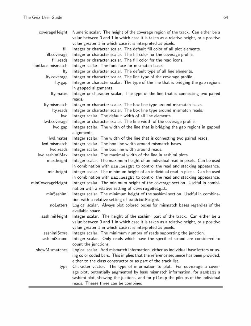
The Gviz User Guide 64
coverageHeight Numeric scalar. The height of the coverage region of the track. Can either be avalue between 0 and 1 in which case it is taken as a relative height, or a positivevalue greater 1 in which case it is interpreted as pixels.
fill Integer or character scalar. The default fill color of all plot elements.fill.coverage Integer or character scalar. The fill color for the coverage profile.
fill.reads Integer or character scalar. The fill color for the read icons.fontface.mismatch Integer scalar. The font face for mismatch bases.
lty Integer or character scalar. The default type of all line elements.lty.coverage Integer or character scalar. The line type of the coverage profile.
lty.gap Integer or character scalar. The type of the line that is bridging the gap regionsin gapped alignments.
lty.mates Integer or character scalar. The type of the line that is connecting two pairedreads.
lty.mismatch Integer or character scalar. The box line type around mismatch bases.lty.reads Integer or character scalar. The box line type around mismatch reads.
lwd Integer scalar. The default width of all line elements.lwd.coverage Integer or character scalar. The line width of the coverage profile.
lwd.gap Integer scalar. The width of the line that is bridging the gap regions in gappedalignments.
lwd.mates Integer scalar. The width of the line that is connecting two paired reads.lwd.mismatch Integer scalar. The box line width around mismatch bases.
lwd.reads Integer scalar. The box line width around reads.lwd.sashimiMax Integer scalar. The maximal width of the line in sashimi plots.
max.height Integer scalar. The maximum height of an individual read in pixels. Can be usedin combination with min.height to control the read and stacking appearance.
min.height Integer scalar. The minimum height of an individual read in pixels. Can be usedin combination with max.height to control the read and stacking appearance.
minCoverageHeight Integer scalar. The minimum height of the coverage section. Uselful in combi-nation with a relative setting of coverageHeight.
minSashimi Integer scalar. The minimum height of the sashimi section. Uselful in combina-tion with a relative setting of sashimiHeight.
noLetters Logical scalar. Always plot colored boxes for mismatch bases regardles of theavailable space.
sashimiHeight Integer scalar. The height of the sashimi part of the track. Can either be avalue between 0 and 1 in which case it is taken as a relative height, or a positivevalue greater 1 in which case it is interpreted as pixels.
sashimiScore Integer scalar. The minimum number of reads supporting the junction.sashimiStrand Integer scalar. Only reads which have the specified strand are considered to
count the junctions.showMismatches Logical scalar. Add mismatch information, either as individual base letters or us-
ing color coded bars. This implies that the reference sequence has been provided,either to the class constructor or as part of the track list.
type Character vactor. The type of information to plot. For coverage a cover-age plot, potentially augmented by base mismatch information, for sashimi asashimi plot, showing the juctions, and for pileup the pileups of the individualreads. Theese three can be combined.
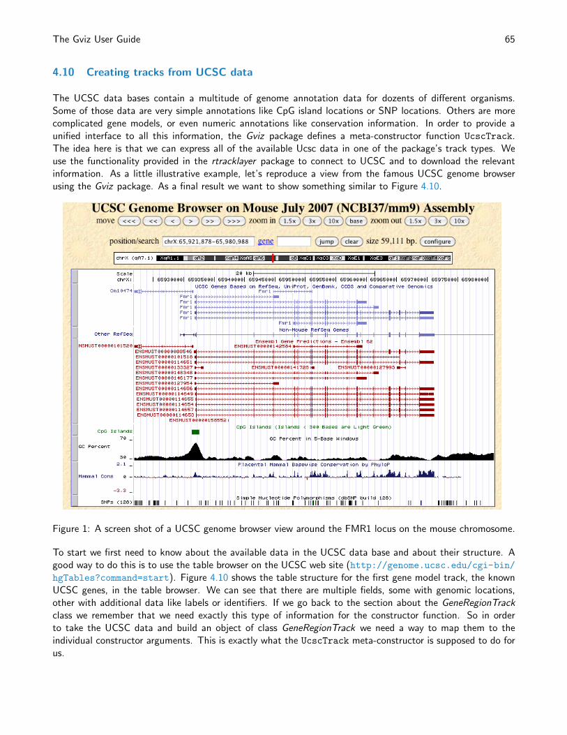
The Gviz User Guide 65
4.10 Creating tracks from UCSC data
The UCSC data bases contain a multitude of genome annotation data for dozents of different organisms.Some of those data are very simple annotations like CpG island locations or SNP locations. Others are morecomplicated gene models, or even numeric annotations like conservation information. In order to provide aunified interface to all this information, the Gviz package defines a meta-constructor function UcscTrack.The idea here is that we can express all of the available Ucsc data in one of the package’s track types. Weuse the functionality provided in the rtracklayer package to connect to UCSC and to download the relevantinformation. As a little illustrative example, let’s reproduce a view from the famous UCSC genome browserusing the Gviz package. As a final result we want to show something similar to Figure 4.10.
Figure 1: A screen shot of a UCSC genome browser view around the FMR1 locus on the mouse chromosome.
To start we first need to know about the available data in the UCSC data base and about their structure. Agood way to do this is to use the table browser on the UCSC web site (http://genome.ucsc.edu/cgi-bin/hgTables?command=start). Figure 4.10 shows the table structure for the first gene model track, the knownUCSC genes, in the table browser. We can see that there are multiple fields, some with genomic locations,other with additional data like labels or identifiers. If we go back to the section about the GeneRegionTrackclass we remember that we need exactly this type of information for the constructor function. So in orderto take the UCSC data and build an object of class GeneRegionTrack we need a way to map them to theindividual constructor arguments. This is exactly what the UcscTrack meta-constructor is supposed to do forus.
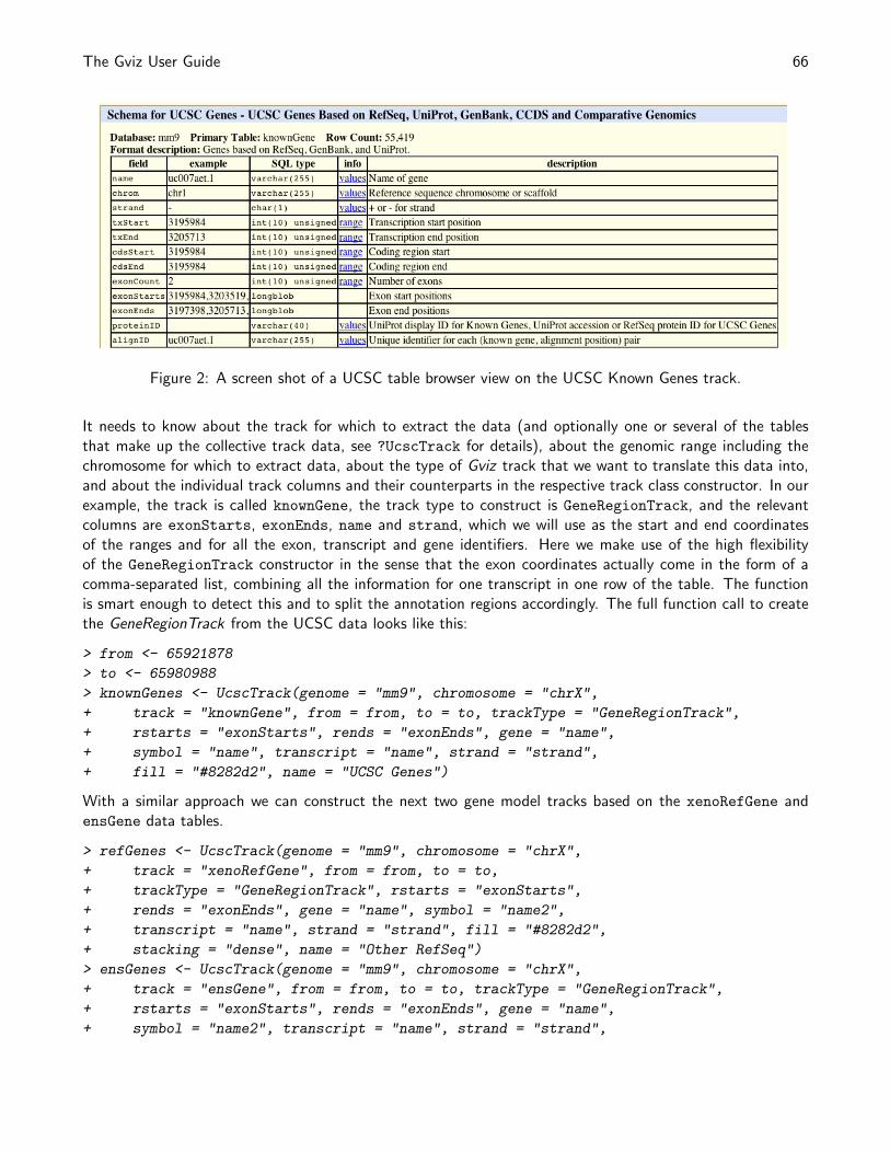
The Gviz User Guide 66
Figure 2: A screen shot of a UCSC table browser view on the UCSC Known Genes track.
It needs to know about the track for which to extract the data (and optionally one or several of the tablesthat make up the collective track data, see ?UcscTrack for details), about the genomic range including thechromosome for which to extract data, about the type of Gviz track that we want to translate this data into,and about the individual track columns and their counterparts in the respective track class constructor. In ourexample, the track is called knownGene, the track type to construct is GeneRegionTrack, and the relevantcolumns are exonStarts, exonEnds, name and strand, which we will use as the start and end coordinatesof the ranges and for all the exon, transcript and gene identifiers. Here we make use of the high flexibilityof the GeneRegionTrack constructor in the sense that the exon coordinates actually come in the form of acomma-separated list, combining all the information for one transcript in one row of the table. The functionis smart enough to detect this and to split the annotation regions accordingly. The full function call to createthe GeneRegionTrack from the UCSC data looks like this:
> from <- 65921878
> to <- 65980988
> knownGenes <- UcscTrack(genome = "mm9", chromosome = "chrX",
+ track = "knownGene", from = from, to = to, trackType = "GeneRegionTrack",
+ rstarts = "exonStarts", rends = "exonEnds", gene = "name",
+ symbol = "name", transcript = "name", strand = "strand",
+ fill = "#8282d2", name = "UCSC Genes")
With a similar approach we can construct the next two gene model tracks based on the xenoRefGene andensGene data tables.
> refGenes <- UcscTrack(genome = "mm9", chromosome = "chrX",
+ track = "xenoRefGene", from = from, to = to,
+ trackType = "GeneRegionTrack", rstarts = "exonStarts",
+ rends = "exonEnds", gene = "name", symbol = "name2",
+ transcript = "name", strand = "strand", fill = "#8282d2",
+ stacking = "dense", name = "Other RefSeq")
> ensGenes <- UcscTrack(genome = "mm9", chromosome = "chrX",
+ track = "ensGene", from = from, to = to, trackType = "GeneRegionTrack",
+ rstarts = "exonStarts", rends = "exonEnds", gene = "name",
+ symbol = "name2", transcript = "name", strand = "strand",
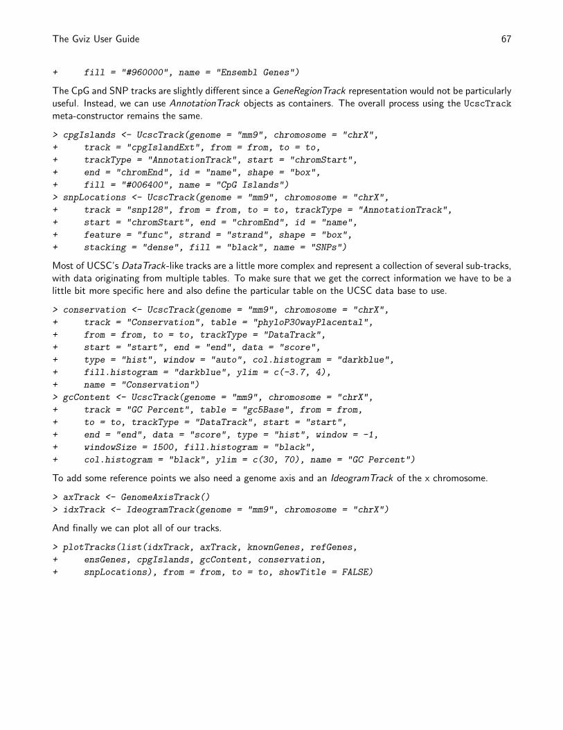
The Gviz User Guide 67
+ fill = "#960000", name = "Ensembl Genes")
The CpG and SNP tracks are slightly different since a GeneRegionTrack representation would not be particularlyuseful. Instead, we can use AnnotationTrack objects as containers. The overall process using the UcscTrack
meta-constructor remains the same.
> cpgIslands <- UcscTrack(genome = "mm9", chromosome = "chrX",
+ track = "cpgIslandExt", from = from, to = to,
+ trackType = "AnnotationTrack", start = "chromStart",
+ end = "chromEnd", id = "name", shape = "box",
+ fill = "#006400", name = "CpG Islands")
> snpLocations <- UcscTrack(genome = "mm9", chromosome = "chrX",
+ track = "snp128", from = from, to = to, trackType = "AnnotationTrack",
+ start = "chromStart", end = "chromEnd", id = "name",
+ feature = "func", strand = "strand", shape = "box",
+ stacking = "dense", fill = "black", name = "SNPs")
Most of UCSC’s DataTrack-like tracks are a little more complex and represent a collection of several sub-tracks,with data originating from multiple tables. To make sure that we get the correct information we have to be alittle bit more specific here and also define the particular table on the UCSC data base to use.
> conservation <- UcscTrack(genome = "mm9", chromosome = "chrX",
+ track = "Conservation", table = "phyloP30wayPlacental",
+ from = from, to = to, trackType = "DataTrack",
+ start = "start", end = "end", data = "score",
+ type = "hist", window = "auto", col.histogram = "darkblue",
+ fill.histogram = "darkblue", ylim = c(-3.7, 4),
+ name = "Conservation")
> gcContent <- UcscTrack(genome = "mm9", chromosome = "chrX",
+ track = "GC Percent", table = "gc5Base", from = from,
+ to = to, trackType = "DataTrack", start = "start",
+ end = "end", data = "score", type = "hist", window = -1,
+ windowSize = 1500, fill.histogram = "black",
+ col.histogram = "black", ylim = c(30, 70), name = "GC Percent")
To add some reference points we also need a genome axis and an IdeogramTrack of the x chromosome.
> axTrack <- GenomeAxisTrack()
> idxTrack <- IdeogramTrack(genome = "mm9", chromosome = "chrX")
And finally we can plot all of our tracks.
> plotTracks(list(idxTrack, axTrack, knownGenes, refGenes,
+ ensGenes, cpgIslands, gcContent, conservation,
+ snpLocations), from = from, to = to, showTitle = FALSE)
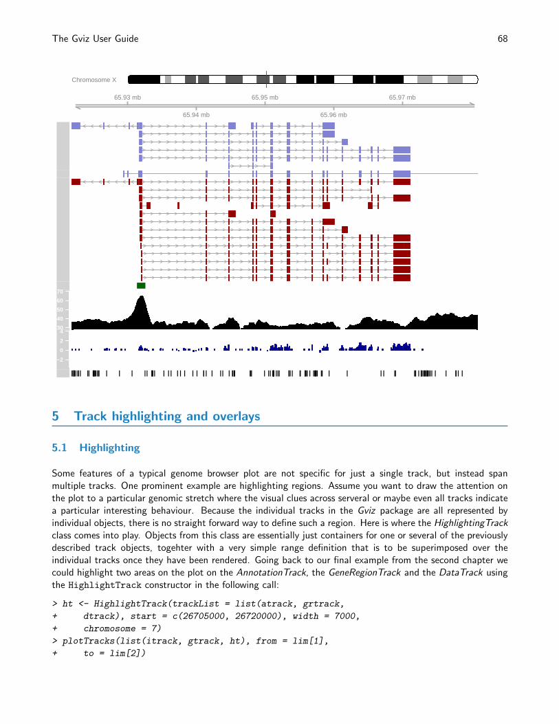
The Gviz User Guide 68
Chromosome X
65.93 mb
65.94 mb
65.95 mb
65.96 mb
65.97 mb
30
40
50
60
70
−2
0
2
4
5 Track highlighting and overlays
5.1 Highlighting
Some features of a typical genome browser plot are not specific for just a single track, but instead spanmultiple tracks. One prominent example are highlighting regions. Assume you want to draw the attention onthe plot to a particular genomic stretch where the visual clues across serveral or maybe even all tracks indicatea particular interesting behaviour. Because the individual tracks in the Gviz package are all represented byindividual objects, there is no straight forward way to define such a region. Here is where the HighlightingTrackclass comes into play. Objects from this class are essentially just containers for one or several of the previouslydescribed track objects, togehter with a very simple range definition that is to be superimposed over theindividual tracks once they have been rendered. Going back to our final example from the second chapter wecould highlight two areas on the plot on the AnnotationTrack, the GeneRegionTrack and the DataTrack usingthe HighlightTrack constructor in the following call:
> ht <- HighlightTrack(trackList = list(atrack, grtrack,
+ dtrack), start = c(26705000, 26720000), width = 7000,
+ chromosome = 7)
> plotTracks(list(itrack, gtrack, ht), from = lim[1],
+ to = lim[2])
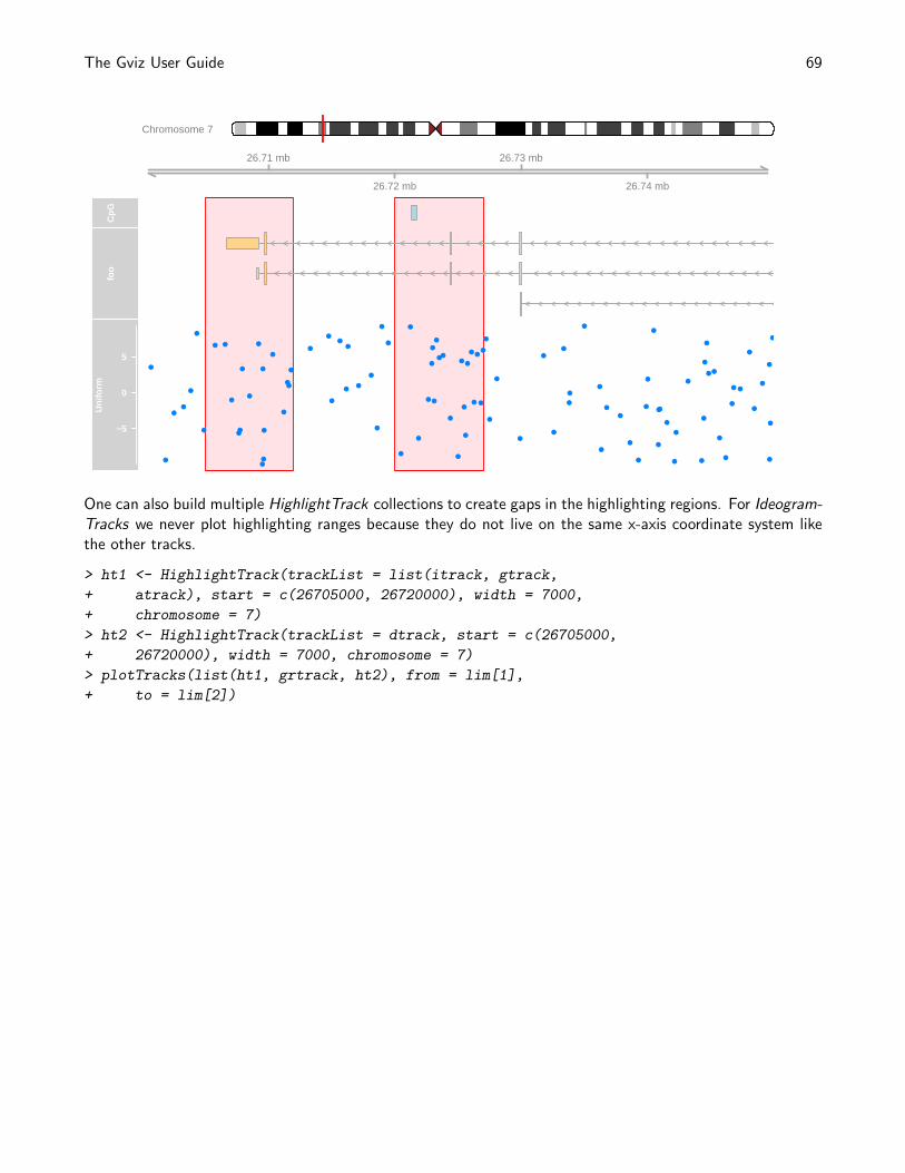
The Gviz User Guide 69
Chromosome 7
26.71 mb
26.72 mb
26.73 mb
26.74 mb
CpG
foo
−5
0
5
Uni
form
●
●
●
●
●
●
●
● ●
●
●●
●
●
●
●
●
●
●
●
●
●●
●
●
●
●
●
●
●
●
●
●
●
●
●
●
●
●
●
●
●
●
●●
●
●
●
●
●
●
●
●
●
●
●
●
●
●
●
●
●
●
●
●
●
●
●
●
●
●
●
●
●
●
●
●●
●
●
●
●
●
●
●
●
● ●
●
●
●
● ●
●
●
●
●
●
●
●
One can also build multiple HighlightTrack collections to create gaps in the highlighting regions. For Ideogram-Tracks we never plot highlighting ranges because they do not live on the same x-axis coordinate system likethe other tracks.
> ht1 <- HighlightTrack(trackList = list(itrack, gtrack,
+ atrack), start = c(26705000, 26720000), width = 7000,
+ chromosome = 7)
> ht2 <- HighlightTrack(trackList = dtrack, start = c(26705000,
+ 26720000), width = 7000, chromosome = 7)
> plotTracks(list(ht1, grtrack, ht2), from = lim[1],
+ to = lim[2])
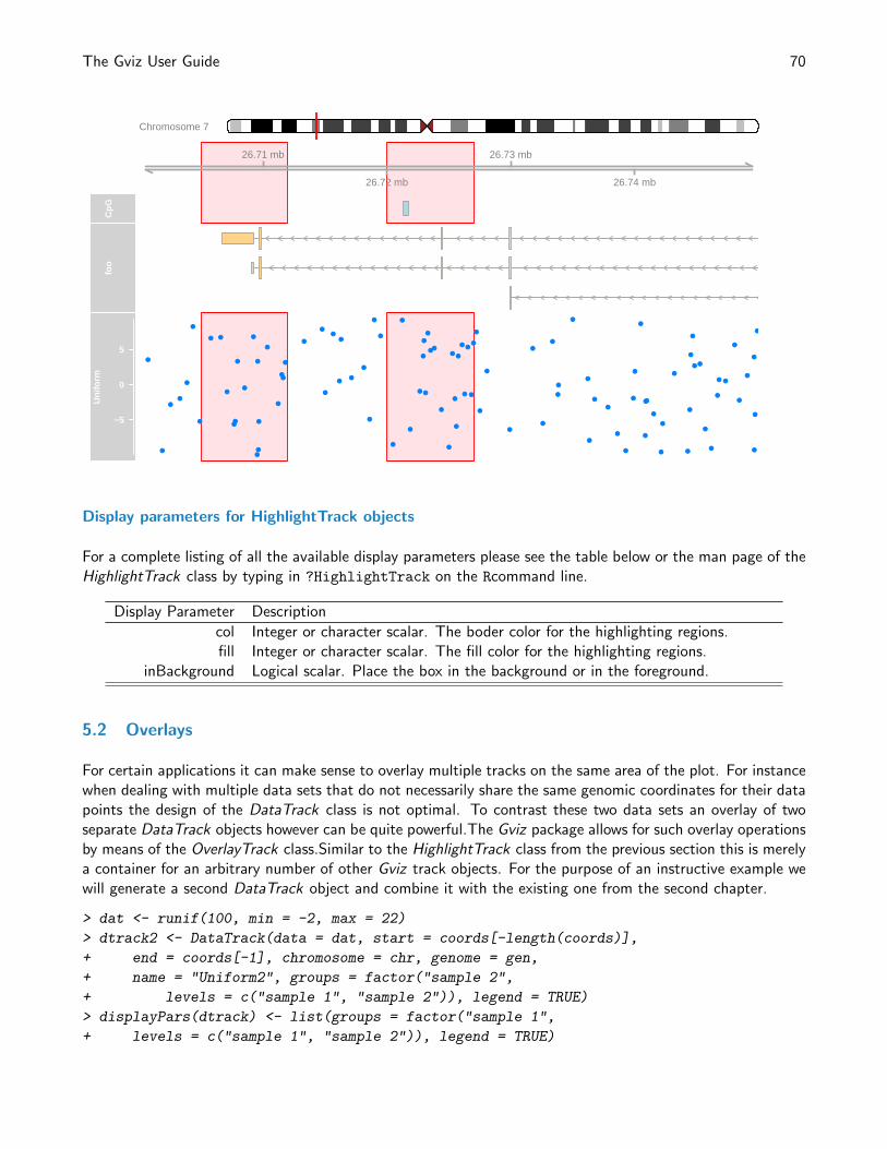
The Gviz User Guide 70
Chromosome 7
26.71 mb
26.72 mb
26.73 mb
26.74 mb
CpG
foo
−5
0
5
Uni
form
●
●
●
●
●
●
●
● ●
●
●●
●
●
●
●
●
●
●
●
●
●●
●
●
●
●
●
●
●
●
●
●
●
●
●
●
●
●
●
●
●
●
●●
●
●
●
●
●
●
●
●
●
●
●
●
●
●
●
●
●
●
●
●
●
●
●
●
●
●
●
●
●
●
●
●●
●
●
●
●
●
●
●
●
● ●
●
●
●
● ●
●
●
●
●
●
●
●
Display parameters for HighlightTrack objects
For a complete listing of all the available display parameters please see the table below or the man page of theHighlightTrack class by typing in ?HighlightTrack on the Rcommand line.
Display Parameter Description
col Integer or character scalar. The boder color for the highlighting regions.fill Integer or character scalar. The fill color for the highlighting regions.
inBackground Logical scalar. Place the box in the background or in the foreground.
5.2 Overlays
For certain applications it can make sense to overlay multiple tracks on the same area of the plot. For instancewhen dealing with multiple data sets that do not necessarily share the same genomic coordinates for their datapoints the design of the DataTrack class is not optimal. To contrast these two data sets an overlay of twoseparate DataTrack objects however can be quite powerful.The Gviz package allows for such overlay operationsby means of the OverlayTrack class.Similar to the HighlightTrack class from the previous section this is merelya container for an arbitrary number of other Gviz track objects. For the purpose of an instructive example wewill generate a second DataTrack object and combine it with the existing one from the second chapter.
> dat <- runif(100, min = -2, max = 22)
> dtrack2 <- DataTrack(data = dat, start = coords[-length(coords)],
+ end = coords[-1], chromosome = chr, genome = gen,
+ name = "Uniform2", groups = factor("sample 2",
+ levels = c("sample 1", "sample 2")), legend = TRUE)
> displayPars(dtrack) <- list(groups = factor("sample 1",
+ levels = c("sample 1", "sample 2")), legend = TRUE)
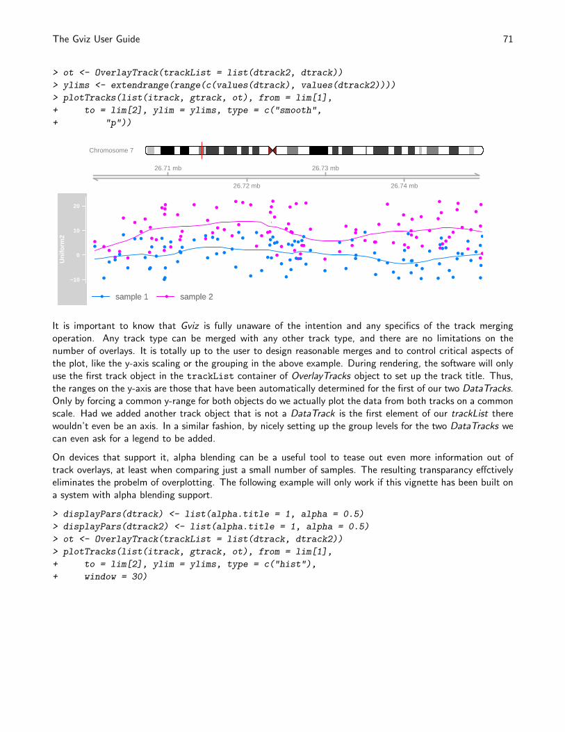
The Gviz User Guide 71
> ot <- OverlayTrack(trackList = list(dtrack2, dtrack))
> ylims <- extendrange(range(c(values(dtrack), values(dtrack2))))
> plotTracks(list(itrack, gtrack, ot), from = lim[1],
+ to = lim[2], ylim = ylims, type = c("smooth",
+ "p"))
Chromosome 7
26.71 mb
26.72 mb
26.73 mb
26.74 mb
−10
0
10
20
Uni
form
2
●
●
●
●
●
●
●
●
●
●
●
●
● ●
●
●
●
●
●
●
●
●●
●
●
●
●
●
●
●●
●
●
●
●●
●
●●●
●
●
●
●
●
●
●
●
●
●●
●
●
●
●
●●
●
●
●
●
●
●
●●
●●●
●
●
●
●
●
●●
●
●
●
●
●
●
●
●
●
●
●
●●
●
●
●
●
●
●
●
●
●
●
●
●
● sample 1 ● sample 2
●
●
●●
●
●
●
● ●
●
●●
●
●
●
●
●
●
●
●
●
●●
●
●
●
●
●
●
●
●●
●
●
●
●
●
●
●
●
●
●
●
●●
●
●
●
●
●
●
●
●
●
●
●
●
●
●
●
●
●
●
●●
●
●
●
●●
●
●
●
●
●
●
●●
●
●
●
●
●
●
●
●
● ●
●
●
●
● ●
●
●
●
●
●
●
●
● sample 1 ● sample 2
It is important to know that Gviz is fully unaware of the intention and any specifics of the track mergingoperation. Any track type can be merged with any other track type, and there are no limitations on thenumber of overlays. It is totally up to the user to design reasonable merges and to control critical aspects ofthe plot, like the y-axis scaling or the grouping in the above example. During rendering, the software will onlyuse the first track object in the trackList container of OverlayTracks object to set up the track title. Thus,the ranges on the y-axis are those that have been automatically determined for the first of our two DataTracks.Only by forcing a common y-range for both objects do we actually plot the data from both tracks on a commonscale. Had we added another track object that is not a DataTrack is the first element of our trackList therewouldn’t even be an axis. In a similar fashion, by nicely setting up the group levels for the two DataTracks wecan even ask for a legend to be added.
On devices that support it, alpha blending can be a useful tool to tease out even more information out oftrack overlays, at least when comparing just a small number of samples. The resulting transparancy effctivelyeliminates the probelm of overplotting. The following example will only work if this vignette has been built ona system with alpha blending support.
> displayPars(dtrack) <- list(alpha.title = 1, alpha = 0.5)
> displayPars(dtrack2) <- list(alpha.title = 1, alpha = 0.5)
> ot <- OverlayTrack(trackList = list(dtrack, dtrack2))
> plotTracks(list(itrack, gtrack, ot), from = lim[1],
+ to = lim[2], ylim = ylims, type = c("hist"),
+ window = 30)
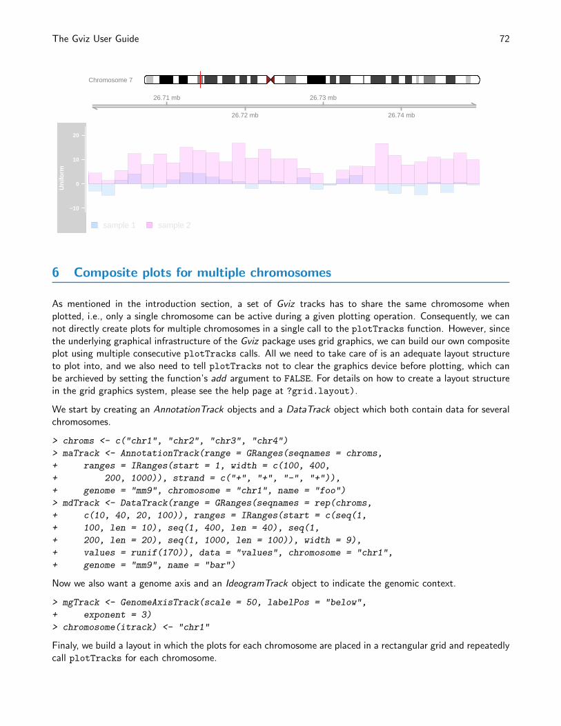
The Gviz User Guide 72
Chromosome 7
26.71 mb
26.72 mb
26.73 mb
26.74 mb
−10
0
10
20
Uni
form
sample 1 sample 2sample 1 sample 2
6 Composite plots for multiple chromosomes
As mentioned in the introduction section, a set of Gviz tracks has to share the same chromosome whenplotted, i.e., only a single chromosome can be active during a given plotting operation. Consequently, we cannot directly create plots for multiple chromosomes in a single call to the plotTracks function. However, sincethe underlying graphical infrastructure of the Gviz package uses grid graphics, we can build our own compositeplot using multiple consecutive plotTracks calls. All we need to take care of is an adequate layout structureto plot into, and we also need to tell plotTracks not to clear the graphics device before plotting, which canbe archieved by setting the function’s add argument to FALSE. For details on how to create a layout structurein the grid graphics system, please see the help page at ?grid.layout).
We start by creating an AnnotationTrack objects and a DataTrack object which both contain data for severalchromosomes.
> chroms <- c("chr1", "chr2", "chr3", "chr4")
> maTrack <- AnnotationTrack(range = GRanges(seqnames = chroms,
+ ranges = IRanges(start = 1, width = c(100, 400,
+ 200, 1000)), strand = c("+", "+", "-", "+")),
+ genome = "mm9", chromosome = "chr1", name = "foo")
> mdTrack <- DataTrack(range = GRanges(seqnames = rep(chroms,
+ c(10, 40, 20, 100)), ranges = IRanges(start = c(seq(1,
+ 100, len = 10), seq(1, 400, len = 40), seq(1,
+ 200, len = 20), seq(1, 1000, len = 100)), width = 9),
+ values = runif(170)), data = "values", chromosome = "chr1",
+ genome = "mm9", name = "bar")
Now we also want a genome axis and an IdeogramTrack object to indicate the genomic context.
> mgTrack <- GenomeAxisTrack(scale = 50, labelPos = "below",
+ exponent = 3)
> chromosome(itrack) <- "chr1"
Finaly, we build a layout in which the plots for each chromosome are placed in a rectangular grid and repeatedlycall plotTracks for each chromosome.
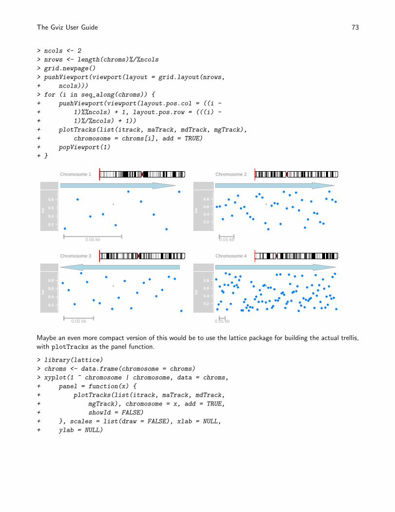
The Gviz User Guide 73
> ncols <- 2
> nrows <- length(chroms)%/%ncols
> grid.newpage()
> pushViewport(viewport(layout = grid.layout(nrows,
+ ncols)))
> for (i in seq_along(chroms)) {
+ pushViewport(viewport(layout.pos.col = ((i -
+ 1)%%ncols) + 1, layout.pos.row = (((i) -
+ 1)%/%ncols) + 1))
+ plotTracks(list(itrack, maTrack, mdTrack, mgTrack),
+ chromosome = chroms[i], add = TRUE)
+ popViewport(1)
+ }
Chromosome 1
0.2
0.4
0.6
0.8
bar
●
●
●●
●
●
●
●
●
●
0.05 kb
Chromosome 2
0.2
0.4
0.6
0.8ba
r ● ●
●
●
●
●
●
●
●●
●
●●
●●
●
●
●
●● ●
●
●
●
●
●
●
●
●
●
●
●
● ●
●●
●
●
●●
0.05 kb
Chromosome 3
0.2
0.4
0.6
0.8
bar
●
●
●
●
●
●
●
●
●
●
●
●
●
●
●
●
●
●●
●
0.05 kb
Chromosome 4
0.2
0.4
0.6
0.8
bar
●
●
●
●
●
●●
●
●
●
●
●
●
●
●
●
●
●●
●
●
●●
●●
●●
●
●
●
●
●
●●
●
●
●
●
●
●●
●
●
●
●
●
●●
●
●
●
●●
●
●●●
●
●●
●
●
●
●●
●
●
●
●
●
●
●
●
●
●
●
●●●
●
●
●
●
●
●
●
●
●
●
●
●
●
●
●
●
●
●
●
●
●
0.05 kb
Maybe an even more compact version of this would be to use the lattice package for building the actual trellis,with plotTracks as the panel function.
> library(lattice)
> chroms <- data.frame(chromosome = chroms)
> xyplot(1 ~ chromosome | chromosome, data = chroms,
+ panel = function(x) {
+ plotTracks(list(itrack, maTrack, mdTrack,
+ mgTrack), chromosome = x, add = TRUE,
+ showId = FALSE)
+ }, scales = list(draw = FALSE), xlab = NULL,
+ ylab = NULL)
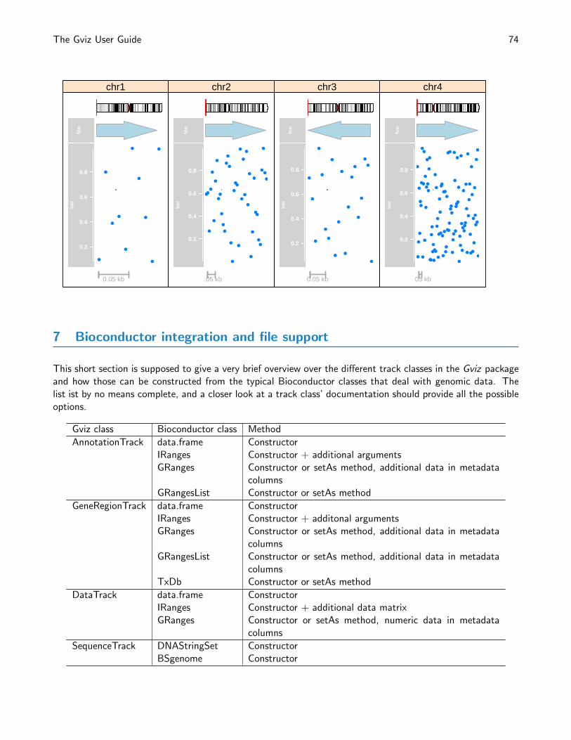
The Gviz User Guide 74
foo
0.2
0.4
0.6
0.8
bar
●
●
●
●
●
●
●
●
●
●
0.05 kb
chr1
foo
0.2
0.4
0.6
0.8ba
r
●●
●
●
●
●
●
●
●
●
●
●
●
●
●
●
●
●
●
●●
●
●
●
●
●
●
●
●
●
●
●
●●
●
●
●
●
●
●
0.05 kb
chr2
foo
0.2
0.4
0.6
0.8
bar
●
●
●
●
●
●
●
●
●
●
●
●
●
●
●
●
●
●
●
●
0.05 kb
chr3
foo
0.2
0.4
0.6
0.8
bar
●
●
●
●
●
●
●
●
●
●
●
●
●
●
●
●
●
●
●
●
●
●●
●
●
●
●
●
●
●
●
●
●
●
●
●
●
●
●
●●
●
●
●
●
●
●
●
●
●
●
●
●
●
●●
●
●
●
●
●
●
●
●●
●
●
●
●
●
●
●
●
●
●
●
●
●●
●
●
●
●
●
●
●
●
●
●
●
●
●
●
●
●
●
●
●
●
●
0.05 kb
chr4
7 Bioconductor integration and file support
This short section is supposed to give a very brief overview over the different track classes in the Gviz packageand how those can be constructed from the typical Bioconductor classes that deal with genomic data. Thelist ist by no means complete, and a closer look at a track class’ documentation should provide all the possibleoptions.
Gviz class Bioconductor class Method
AnnotationTrack data.frame ConstructorIRanges Constructor + additional argumentsGRanges Constructor or setAs method, additional data in metadata
columnsGRangesList Constructor or setAs method
GeneRegionTrack data.frame ConstructorIRanges Constructor + additonal argumentsGRanges Constructor or setAs method, additional data in metadata
columnsGRangesList Constructor or setAs method, additional data in metadata
columnsTxDb Constructor or setAs method
DataTrack data.frame ConstructorIRanges Constructor + additional data matrixGRanges Constructor or setAs method, numeric data in metadata
columns
SequenceTrack DNAStringSet ConstructorBSgenome Constructor
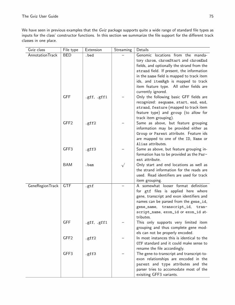
The Gviz User Guide 75
We have seen in previous examples that the Gviz package supports quite a wide range of standard file types asinputs for the class’ constructor functions. In this section we summarize the file support for the different trackclasses in one place.
Gviz class File type Extension Streaming Details
AnnotationTrack BED .bed – Genomic locations from the manda-tory chrom, chromStart and chromEnd
fields, and optionally the strand from thestrand field. If present, the informationin the name field is mapped to track itemids, and itemRgb is mapped to trackitem feature type. All other fields arecurrently ignored.
GFF .gff, .gff1 – Only the following basic GFF fields arerecognized: seqname, start, end, end,strand, feature (mapped to track itemfeature type) and group (to allow fortrack item grouping).
GFF2 .gff2 – Same as above, but feature groupinginformation may be provided either asGroup or Parent attribute. Feature idsare mapped to one of the ID, Name orAlias attributes.
GFF3 .gff3 – Same as above, but feature grouping in-formation has to be provided as the Par-ent attribute.
BAM .bam√
Only start and end locations as well asthe strand information for the reads areused. Read identifiers are used for trackitem grouping.
GeneRegionTrack GTF .gtf – A somewhat looser format definitionfor gtf files is applied here wheregene, transcript and exon identifiers andnames can be parsed from the gene_id,gene_name, transcript_id, tran-
script_name, exon_id or exon_id at-tributes.
GFF .gff, .gff1 – This only supports very limited itemgrouping and thus complete gene mod-els can not be properly encoded.
GFF2 .gff2 – In most instances this is identical to theGTF standard and it could make sense torename the file accordingly.
GFF3 .gff3 – The gene-to-transcript and transcript-to-exon relationships are encoded in theparent and type attributes and theparser tries to accomodate most of theexisiting GFF3 variants.
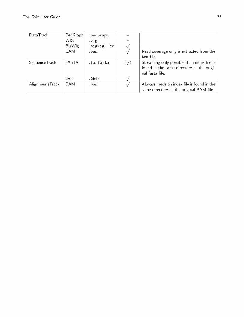
The Gviz User Guide 76
DataTrack BedGraph .bedGraph –WIG .wig –BigWig .bigWig, .bw
√
BAM .bam√
Read coverage only is extracted from thebam file.
SequenceTrack FASTA .fa, fasta (√) Streaming only possible if an index file is
found in the same directory as the origi-nal fasta file.
2Bit .2bit√
AlignmentsTrack BAM .bam√
ALways needs an index file is found in thesame directory as the original BAM file.
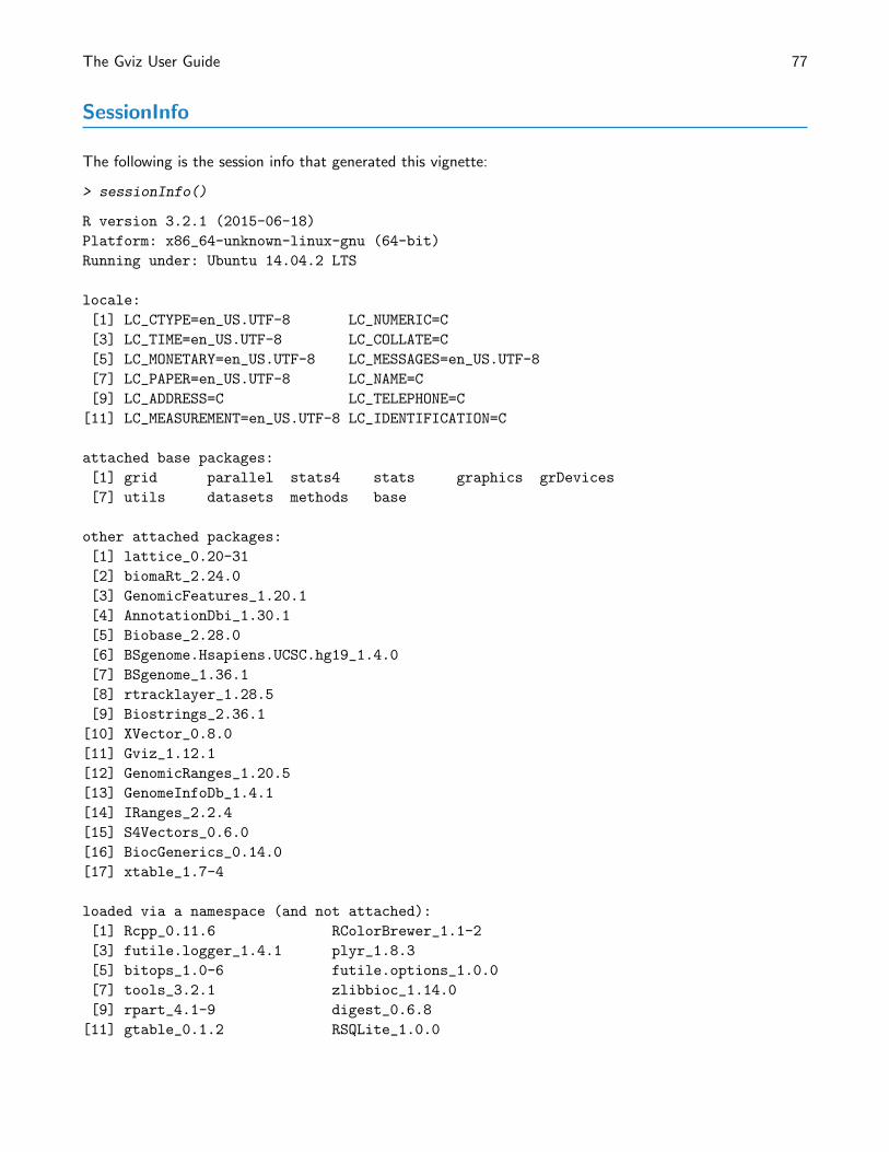
The Gviz User Guide 77
SessionInfo
The following is the session info that generated this vignette:
> sessionInfo()
R version 3.2.1 (2015-06-18)
Platform: x86_64-unknown-linux-gnu (64-bit)
Running under: Ubuntu 14.04.2 LTS
locale:
[1] LC_CTYPE=en_US.UTF-8 LC_NUMERIC=C
[3] LC_TIME=en_US.UTF-8 LC_COLLATE=C
[5] LC_MONETARY=en_US.UTF-8 LC_MESSAGES=en_US.UTF-8
[7] LC_PAPER=en_US.UTF-8 LC_NAME=C
[9] LC_ADDRESS=C LC_TELEPHONE=C
[11] LC_MEASUREMENT=en_US.UTF-8 LC_IDENTIFICATION=C
attached base packages:
[1] grid parallel stats4 stats graphics grDevices
[7] utils datasets methods base
other attached packages:
[1] lattice_0.20-31
[2] biomaRt_2.24.0
[3] GenomicFeatures_1.20.1
[4] AnnotationDbi_1.30.1
[5] Biobase_2.28.0
[6] BSgenome.Hsapiens.UCSC.hg19_1.4.0
[7] BSgenome_1.36.1
[8] rtracklayer_1.28.5
[9] Biostrings_2.36.1
[10] XVector_0.8.0
[11] Gviz_1.12.1
[12] GenomicRanges_1.20.5
[13] GenomeInfoDb_1.4.1
[14] IRanges_2.2.4
[15] S4Vectors_0.6.0
[16] BiocGenerics_0.14.0
[17] xtable_1.7-4
loaded via a namespace (and not attached):
[1] Rcpp_0.11.6 RColorBrewer_1.1-2
[3] futile.logger_1.4.1 plyr_1.8.3
[5] bitops_1.0-6 futile.options_1.0.0
[7] tools_3.2.1 zlibbioc_1.14.0
[9] rpart_4.1-9 digest_0.6.8
[11] gtable_0.1.2 RSQLite_1.0.0
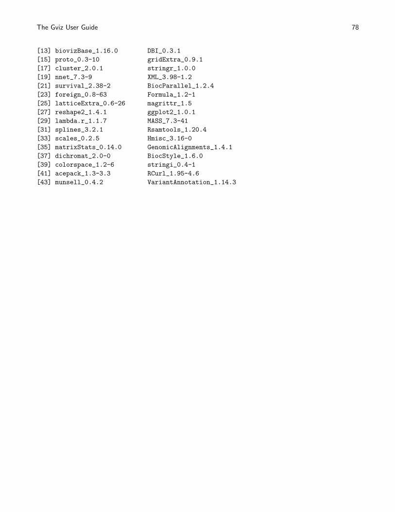
The Gviz User Guide 78
[13] biovizBase_1.16.0 DBI_0.3.1
[15] proto_0.3-10 gridExtra_0.9.1
[17] cluster_2.0.1 stringr_1.0.0
[19] nnet_7.3-9 XML_3.98-1.2
[21] survival_2.38-2 BiocParallel_1.2.4
[23] foreign_0.8-63 Formula_1.2-1
[25] latticeExtra_0.6-26 magrittr_1.5
[27] reshape2_1.4.1 ggplot2_1.0.1
[29] lambda.r_1.1.7 MASS_7.3-41
[31] splines_3.2.1 Rsamtools_1.20.4
[33] scales_0.2.5 Hmisc_3.16-0
[35] matrixStats_0.14.0 GenomicAlignments_1.4.1
[37] dichromat_2.0-0 BiocStyle_1.6.0
[39] colorspace_1.2-6 stringi_0.4-1
[41] acepack_1.3-3.3 RCurl_1.95-4.6
[43] munsell_0.4.2 VariantAnnotation_1.14.3

The Gviz User Guide 79
References
[1] Yarden Katz, Eric T. Wang, Jacob Silterra, Schraga Schwartz, Bang Wong, Helga Thorvaldsdottir,James T. Robinson, Jill P. Mesirov, Edoardo M. Airoldi, and Christopher B. Burge. Quantita-tive visualization of alternative exon expression from rna-seq data. Bioinformatics, 2015. URL:http://bioinformatics.oxfordjournals.org/content/early/2015/02/25/bioinformatics.
btv034.abstract, arXiv:http://bioinformatics.oxfordjournals.org/content/early/2015/
02/25/bioinformatics.btv034.full.pdf+html, doi:10.1093/bioinformatics/btv034.


![Beyond the shot [the cinematographic principle & the ideogram]](https://img.pdfslide.us/doc/110x75/56816581550346895dd81c95/beyond-the-shot-the-cinematographic-principle-the-ideogram.jpg)