Federal Reserve Bank of Minneapolis Quarterly ReviewWinter 1999, vol. 23, no. 1, pp. 2–24

The Great Depression in the United StatesFrom A Neoclassical Perspective

Harold L. Cole Lee E. OhanianSenior Economist EconomistResearch Department Research DepartmentFederal Reserve Bank of Minneapolis Federal Reserve Bank of Minneapolis

Abstract

Can neoclassical theory account for the Great Depression in the United States—both the downturn in output between 1929 and 1933 and the recovery between1934 and 1939? Yes and no. Given the large real and monetary shocks to the U.S.economy during 1929–33, neoclassical theory does predict a long, deep downturn.However, theory predicts a much different recovery from this downturn thanactually occurred. Given the period’s sharp increases in total factor productivityand the money supply and the elimination of deflation and bank failures, theorypredicts an extremely rapid recovery that returns output to trend around 1936. Insharp contrast, real output remained between 25 and 30 percent below trendthrough the late 1930s. We conclude that a new shock is needed to account for theDepression’s weak recovery. A likely culprit is New Deal policies toward monop-oly and the distribution of income.

The views expressed herein are those of the authors and not necessarily those of the FederalReserve Bank of Minneapolis or the Federal Reserve System.

Between 1929 and 1933, employment fell about 25 per-cent and output fell about 30 percent in the United States.By 1939, employment and output remained well belowtheir 1929 levels. Why did employment and output fall somuch in the early 1930s? Why did they remain so low adecade later?

In this article, we address these two questions by eval-uating macroeconomic performance in the United Statesfrom 1929 to 1939. This period consists of adeclinein eco-nomic activity (1929–33) followed by arecovery(1934–39). Our definition of theGreat Depressionas a 10-yearevent differs from the standard definition of the Great De-pression, which is the 1929–33 decline. We define the De-pression this way because employment and output re-mained well below their 1929 levels in 1939.

We examine the Depression from the perspective ofneoclassical growth theory. Byneoclassical growth theory,we mean the optimal growth model in Cass 1965 andKoopmans 1965augmentedwith variousshocks that causeemployment and output to deviate from their deterministicsteady-state paths as in Kydland and Prescott 1982.1

We use neoclassical growth theory to study macroeco-nomic performance during the 1930s the way other econ-omists have used the theory to study postwar business cy-cles. We first identify a set of shocks considered importantin postwar economic declines: technology shocks, fiscalpolicy shocks, trade shocks, and monetary shocks. We thenask whether those shocks, within the neoclassical frame-work, can account for the decline and the recovery in the1930s. This method allows us to understand which datafrom the 1930s are consistent with neoclassical theory and,especially, which observations are puzzling from the neo-classical perspective.

In our analysis, we treat the 1929–33 decline as a longand severe recession.2 But the neoclassical approach to an-alyzing business cycles is not just to assess declines in eco-nomic activity, but to assess recoveries as well. When wecompare the decline and recovery during the Depression toa typical postwar business cycle, we see striking differ-ences in duration and scale. The decline, as well as the re-covery, during the Depression lasted about four times aslong as the postwar business cycle average. Moreover, thesize of the decline in output in the 1930s was about 10times the size of the average decline. (See Table 1.)

What factors were responsible for these large differ-ences in the duration and scale of the Depression? Onepossibility is that theshocks—the unexpected changes intechnology, preferences, endowments, or government pol-icies that lead output to deviate from its existing steady-state growth path—were different in the 1930s. One viewis that the shocks responsible for the 1929–33 decline weremuch larger and more persistent versions of the sameshocks that are important in shorter and milder declines.Another view is that the types of shocks responsible for the1929–33 decline were fundamentally different from thoseconsidered to be the driving factors behind typical cyclicaldeclines.

To evaluate these two distinct views, we analyze datafrom the 1930s using the neoclassical growth model. Ourmain finding differs from the standard view that the mostpuzzling aspect of the Depression is the large decline be-tween 1929 and 1933. We find that while it may be pos-sible to account for the 1929–33 decline on the basis of the

shocks we consider, none of those shocks can account forthe 1934–39 recovery. Theory predicts large increases inemployment and output beginning in 1934 that return realeconomic activity rapidly to trend. This prediction standsin sharp contrast to the data, suggesting to us that we needa new shock to account for the weak recovery.

We begin our study by examining deviations in outputand inputs from the trend growth that theory predicts in theabsence of any shocks to the economy. This examinationnot only highlights the severity of the economic declinebetween 1929 and 1933, but also raises questions about therecovery that began in 1934. In 1939, real per capita outputremained 11 percent below its 1929 level: output increasesan average of 21 percent during a typical 10-year period.This contrast identifies two challenges for theory: account-ing for the large decline in economic activity that occurredbetween 1929 and 1933 and accounting for the weak re-covery between 1934 and 1939.

We first evaluate the importance ofreal shocks—tech-nology shocks, fiscal policy shocks, and trade shocks—forthis decade-long period. We find that technology shocksmay have contributed to the 1929–33 decline. However,we find that the real shocks predict a very robust recoverybeginning in 1934. Theory suggests that real shocks shouldhave led employment and output to return to trend by1939.

We next analyze whethermonetary shockscan accountfor the decline and recovery. Some economists, such asFriedmanandSchwartz(1963),arguethatmonetaryshockswere a key factor in the 1929–33 decline. To analyze themonetary shock view, we use the well-known model ofLucas and Rapping (1969), which connects changes in themoney supply to changes in output through intertemporalsubstitution of leisure and unexpected changes in wages.The Lucas-Rapping model predicts that monetary shocksreduced output in the early 1930s, but the model also pre-dicts that employment and output should have been backnear trend by the mid-1930s.

Both real shocks and monetary shocks predict that em-ployment and output should have quickly returned to trendlevels. These predictions are difficult to reconcile with theweak 1934–39 recovery. If the factors considered impor-tant in postwar fluctuations can’t fully account for macro-economic performance in the 1930s, are there other factorsthat can? We go on to analyze two other factors that someeconomists consider important in understanding the De-pression:financial intermediation shocksand inflexiblenominal wages. One type of financial intermediation shockis the bank failures that occurred during the early 1930s.Some researchers argue that these failures reduced outputby disrupting financial intermediation. While bank failuresperhaps deepened the decline, we argue that their impactwould have been short-lived and, consequently, that bankfailures were not responsible for the weak recovery. An-other type of financial intermediation shock is the increasesin reserve requirements that occurred in late 1936 and early1937. While this change may have led to a small declinein output in 1937, it cannot account for the weak recoveryprior to 1937 and cannot account for the significant dropin activity in 1939 relative to 1929.

The other alternative factor is inflexible nominal wages.The view of this factor holds that nominal wages were notas flexible as prices and that the fall in the price level

raised real wages and reduced employment. We presentdata showing that manufacturing real wages rose consis-tently during the 1930s, but that nonmanufacturing wagesfell. The 10-year increase in manufacturing wages is dif-ficult to reconcile with nominal wage inflexibility, whichtypically assumes that inflexibility is due to either moneyillusion or explicit nominal contracts. The long duration ofthe Depression casts doubt on both of these determinantsof inflexible nominal wages.

The weak recovery is a puzzle from the perspective ofneoclassical growth theory. Our inability to account for therecovery with these shocks suggests to us that an alterna-tive shock is important for understanding macroeconomicperformance after 1933. We conclude our study by con-jecturing that government policies toward monopoly andthe distribution of income are a good candidate for thisshock. The National Industrial Recovery Act (NIRA) of1933 allowed much of the economy to cartelize. This pol-icy change would have depressed employment and outputin those sectors covered by the act and, consequently, haveled to a weak recovery. Whether the NIRA can quantita-tively account for the weak recovery is an open questionfor future research.

The Data Through the Lens of the TheoryNeoclassical growth theory has two cornerstones: the ag-gregate production technology, which describes how laborand capital services are combined to create output, and thewillingness and ability of households to substitute com-modities over time, which govern how households allocatetheir time between market and nonmarket activities andhow households allocate their income between consump-tion and savings. Viewed through the lens of this theory,the following variables are keys to understanding macro-economic performance: the allocation of output betweenconsumption and investment, the allocation of time (laborinput) between market and nonmarket activities, and pro-ductivity.3

OutputIn Table 2, we compare levels of output during the De-pression to peak levels in 1929. To do this, we present dataon consumption and investment and the other componentsof real gross national product (GNP) for the 1929–39 pe-riod.4 Data are from the national income and product ac-counts published by the Bureau of Economic Analysis ofthe U.S. Department of Commerce. All data are divided bythe working-age(16 years and older) population. Sinceneoclassical growth theory indicates that these variablescan be expected to grow, on average, at the trend rate oftechnology, they are alsodetrended,that is, adjusted fortrend growth.5 With these adjustments, the data can be di-rectly compared to their peak values in 1929.

As we can see in Table 2, all the components ofrealoutput(GNP in base-year prices), except government pur-chases of goods and services, fell considerably during the1930s. The general pattern for the declining series is avery large drop between 1929 and 1933 followed by onlya moderate rise from the 1933 trough. Output fell morethan 38 percent between 1929 and 1933. By 1939, outputremained nearly 27 percent below its 1929 detrended lev-el. This detrended decline of 27 percent consists of a raw11 percent drop in per capita output and a further 16 per-

cent drop representing trend growth that would have nor-mally occurred over the 1929–39 period.6

The largest decline in economic activity occurred inbusiness investment, which fell nearly 80 percent between1929 and 1933. Consumer durables, which representhousehold, as opposed to business, investment, followeda similar pattern, declining more than 55 percent between1929 and 1933. Consumption of nondurables and servicesdeclined almost 29 percent between 1929 and 1933. For-eign trade (exports and imports) also fell considerably be-tween 1929 and 1933. The impact of the decline between1929 and 1933 on government purchases was relativelymild, and government spending even rose above its trendlevel in 1930 and 1931.

Table 2 also makes clear that the economy did not re-cover much from the 1929–33 decline. Although invest-ment improved relative to its 1933 trough level, investmentremained 51 percent below its 1929 (detrended) level in1939. Consumer durables remained 36 percent below their1929 level in 1939. Relative to trend, consumption of non-durables and services increased very little during the re-covery. In 1933, consumption was about 28 percent belowits 1929 detrended level. By 1939, consumption remainedabout 25 percent below this level.

These unique and large changes in economic activityduring the Depression also changed thecompositionofoutput—the shares of output devoted to consumption, in-vestment, government purchases, and exports and imports.These data are presented in Table 3. The share of outputconsumed rose considerably during the early 1930s, whilethe share of output invested, including consumer durables,declined sharply, falling from 25 percent in 1929 to just 8percent in 1932. During the 1934–39 recovery, the shareof output devoted to investment averaged about 15 percent,compared to its postwar average of 20 percent. This lowrate of investment led to a decline in thecapital stock—thegross stock of fixed reproducible private capital declinedmore than 6 percent between 1929 and 1939, representinga decline of more than 25 percent relative to trend. Foreigntrade comprised a small share of economic activity in theUnited States during the 1929–39 period. Both exports andimports accounted for about 4 percent of output during thedecade. The increase in government purchases, combinedwith the decrease in output, increased the government’sshare of output from 13 percent to about 20 percent by1939.

These data raise the possibility that the recovery was aweak one. To shed some light on this possibility, in Table4, we show the recovery from a typical postwar recession.The data in Table 4 are average detrended levels relativeto peak measured quarterly from the trough. A comparisonof Tables 2 and 4 shows that the recovery from a typicalpostwar recession differs considerably from the 1934–39recovery during the Depression. First, output rapidly re-covers to trend following a typical postwar recession. Sec-ond, consumption grows smoothly following a typicalpostwar recession. This contrasts sharply to the flat timepath of consumption during the 1934–39 recovery. Third,investment recovers very rapidly following a typical post-war recession. Despite falling much more than output dur-ing a recession, investment recovers to a level comparableto the output recovery level within three quarters after thetrough. During the Depression, however, the recovery in

investment was much slower, remaining well below therecovery in output.

Tables 2 and 4 indicate that the 1934–39 recovery wasmuch weaker than the recovery from a typical recession.One interpretation of the weak 1934–39 recovery is thatthe economy was not returning to its pre-1929 steady-stategrowth path, but was settling on a considerably lowersteady-state growth path.

The possibility that the economy was converging to alower steady-state growth path is consistent with the factthat consumption fell about 25 percent below trend by1933 and remained near that level for the rest of the de-cade. (See Chart 1.) Consumption is a good barometer ofa possible change in the economy’s steady state becausehousehold dynamic optimization implies that all future ex-pectations of income should be factored into current con-sumption decisions.7

Labor InputData on labor input are presented in Table 5. We useKendrick’s (1961) data on labor input, capital input, pro-ductivity, and output.8 We present five measures of laborinput, each divided by the working-age population. Wedon’t detrend these ratios because theory implies that theywill be constant along the steady-state growth path.9 Here,again, data are expressed relative to their 1929 values.

The three aggregate measures of labor input declinedsharply from 1929 to 1933.Total employment,which con-sists of private and government workers, declined about 24percent between 1929 and 1933 and remained 18 percentbelow its 1929 level in 1939.Total hours,which reflectchanges in employment and changes in hours per worker,declined more sharply than total employment, and thetrough didn’t occur until 1934. Total hours remained 21percent below their 1929 level in 1939.Private hours,which don’t include the hours of government workers, de-clined more sharply than total hours, reflecting the fact thatgovernment employment did not fall during the 1930s.Private hours fell more than 25 percent between 1929 and1939.

These large declines in aggregate labor input reflectdifferent changes across sectors of the economy.Farmhoursandmanufacturing hoursare shown in the last twocolumns of Table 5. In addition to being divided by theworking-age population, the farm hours measure is adjust-ed for an annual secular decline in farm employment ofabout 1.8 percent per year. In contrast to the other mea-sures of labor input, farm hours remained near trend duringmuch of the decade. Farm hours were virtually unchangedbetween 1929 and 1933, a period in which hours workedin other sectors fell sharply. Farm hours did fall about 10percent in 1934 and were about 7 percent below their 1929level by 1939. A very different picture emerges for manu-facturing hours, which plummeted more than 40 percentbetween 1929 and 1933 and remained 22 percent belowtheir detrended 1929 level at the end of the decade.

These data indicate important differences between thefarm and manufacturing sectors during the Depression.Why didn’t farm hours decline more during the Depres-sion? Why did manufacturing hours decline so much?

Finally, note that the changes in nonfarm labor input aresimilar to changes in consumption during the 1930s. Inparticular, after falling sharply between 1929 and 1933,measures of labor input remained well below 1929 levels

in 1939. Thus, aggregate labor input data also suggest thatthe economy was settling on a growth path lower than thepath the economy was on in 1929.

ProductivityIn Table 6, we present two measures of productivity:laborproductivity(output per hour) andtotal factor productivity.Both measures are detrended and expressed relative to1929 measures. These two series show similar changesduring the 1930s. Labor productivity and total factor pro-ductivity both declined sharply in 1932 and 1933, fallingabout 12 percent and 14 percent, respectively, below their1929 detrended levels. After 1933, however, both mea-sures rose quickly relative to trend and, in fact, returned totrend by 1936. When we compare 1939 data to 1929 data,we see that the 1930s were a decade of normal productivi-ty growth. Labor productivity grew more than 22 percentbetween 1929 and 1939, and total factor productivity grewmore than 20 percent in the same period. This normalgrowth in productivity raises an important question aboutthe lack of a recovery in hours worked, consumption, andinvestment. In the absence of a large negative shift in thelong-run path of productivity, why would the economy beon a lower steady-state growth path in 1939?

An International ComparisonMany countries suffered economic declines during the1930s; however, there are two important distinctions be-tween economic activity in the United States and othercountries during the 1930s. The decline in the UnitedStates was much more severe, and the recovery from thedecline was weaker. To see this, we examine average realper capita output relative to its 1929 level for Belgium,Britain, France, Germany, Italy, Japan, and Sweden. Thedata are from Maddison 1991 and are normalized for eachcountry so that per capita output is equal to 100 in 1929.Since there is some debate over the long-run growth ratein some of these countries, we have not detrended the data.

Table 7 shows the U.S. data and the mean of the nor-malized data for other countries. The total drop in outputis relatively small in other countries: an 8.7 percent dropcompared to a 33.3 percent drop in the United States. Theinternational economies recovered quickly: output in mostcountries returned to 1929 levels by 1935 and was abovethose levels by 1938. Employment also generally recov-ered to its 1929 level by 1938.10

While accounting for other countries’ economic de-clines is beyond the scope of this analysis, we can drawtwo conclusions from this comparison. First, the larger de-cline in the United States is consistent with the view thatthe shocks that caused the decline in the United Stateswere larger than the shocks that caused the decline in theother countries. Second, the weak recovery in the UnitedStates is consistent with the view that the shocks that im-peded the U.S. recovery did not affect most other coun-tries. Instead, the post-1933 shock seems to be largely spe-cific to the United States.

The data we’ve examined so far suggest that inputs andoutput in the United States fell considerably during the1930s and did not recover much relative to the increase inproductivity. Moreover, the data show that the decline wasmuch more severe and the recovery weaker in the UnitedStates than in other countries. To account for the decade-long Depression in the United States, we conclude that we

should focus on domestic, rather than international, factors.We turn to this task in the next section.

Can Real Shocks Account for the Depression?Neoclassical theory and the data have implications for theplausibility of different sources of real shocks in account-ing for the Depression. Since the decline in output was solarge and persistent, we will look for large and persistentnegative shocks. We analyze three classes of real shocksconsidered important in typical business cycle fluctuations:technology shocks, fiscal policy shocks, and trade shocks.

Technology Shocks? Perhaps InitiallyFirst we considertechnology shocks,defined as any exog-enous factor that changes the efficiency with which busi-ness enterprises transform inputs into output. Under thisbroad definition of technology shocks, changes in produc-tivity reflect not only true changes in technology, but alsosuch other factors as changes in work rules and practicesor government regulations that affect the efficiency of pro-duction but are exogenous from the perspective of businessenterprises.Howdotechnologyshocksaffecteconomicac-tivity? The key element that leads to a decline in economicactivity in models with technology shocks is a negativeshock that reduces the marginal products of capital and la-bor. Shocks that reduce the efficiency of transforming in-puts into output lead households to substitute out of marketactivities into nonmarket activities and result in lower out-put. Recent research has identified these shocks as impor-tant factors in postwar business cycle fluctuations. Prescott(1986), for example, shows that a standard one-sector neo-classical model with a plausibly parameterized stochasticprocess for technology shocks can account for 70 percentof postwar business cycle fluctuations. Can technologyshocks account for the Depression?

If these shocks were responsible, we should see a largeand persistent drop intechnology—the efficiency of trans-forming inputs into output—during the 1930s. To see ifsuch a drop occurred, we first need a measure of technol-ogy for this period. Under the neoclassical assumptions ofconstant returns to scale in production and perfectly com-petitive markets, theory implies that changes in total factorproductivity are measures of changes in technology. Thedata do show a drop in total factor productivity—a 14 per-cent (detrended) drop between 1929 and 1933 followed bya rapid recovery. What is the quantitative importance ofthese changes in accounting for the Depression?

To address this question, we present the prediction foroutput for 1930–39 from a real business cycle model. (SeeHansen 1985, Prescott 1986, or King, Plosser, and Rebelo1988 for a discussion of this model.) Our model consists ofequations (A1)–(A5) and (A9) in the Appendix, alongwith the following preference specification:

(1) u(ct,lt) = log(ct) + A log(lt).

We use the following Cobb-Douglas production functionspecification:

(2) zt f(kt,nt) = ztkθt(xtnt)

1−θ.

The household has one unit of time available each period:

(3) 1 = lt + nt.

And we use the following specification of the stochasticprocess for the technology shock:

(4) zt = (1−ρ) + ρzt−1 + εt , εt ~ N(0,σ2).

With values for the parameters of the model, we can usenumerical methods to compute an approximate solution tothe equilibrium of this economy.11 We setθ = 0.33 to con-form to the observation that capital income is about one-third of output. We setσ = 1.7 percent andρ = 0.9 to con-form to the observed standard deviation and serial correla-tion of total factor productivity. We choose the value forthe parameterA so that households spend about one-thirdof their discretionary time working in the deterministicsteady state. Labor-augmenting technological change (xt)grows at a rate of 1.9 percent per year. The population(nt)grows at a rate of 1 percent per year. We set the deprecia-tion rate at 10 percent per year.

We conduct the analysis by assuming that the capitalstock in 1929 is equal to its steady-state value, and then wefeed in the sequence of observed levels of total factor pro-ductivity as measures of the technology shock. Given theinitial condition and the time path of technology, the modelpredicts labor input, output, consumption, and investmentfor each year during the 1930s. We summarize the resultsof the analysis in Chart 2, where we plot the detrendedpredicted level of output from the model between 1929and 1939. For comparison, we also plot the actual detrend-ed level of output. Note that the model predicts a signifi-cant decline in output between 1929 and 1933, althoughthe decline is not as large as the observed decline in thedata: a 15 percent predicted decline compared to a 38 per-cent actual decline. Further, note that as a consequence ofrapid growth in total factor productivity after 1934, themodel predicts a rapid recovery: output should have re-turned to trend by 1936. In contrast, actual output remainedabout 25 percent below trend during the recovery.

One factor that may be contributing to the rapid recov-ery in the model is the fact that the capital stock in themodel falls less than in the data. Consequently, output pre-dicted by the model may be relatively high because thecapital stock is high. To correct for this difference, we con-duct another analysis in which we also feed in the se-quence of total factor productivity measures between 1934and 1939, but we use the actual capital stock in 1934 (20percent below trend) as the initial condition for 1934. Chart3 shows that this change reduces output predicted by themodel by about 3 percent at the beginning of the recovery.But because the initial capital stock in this analysis is low-er, the marginal product of capital is higher, and the pre-dicted rate of output growth in the recovery is faster thanin the first analysis. This recovery brings output back to itstrend level by 1937. The predicted output level is about 27percent above the actual data level in 1939.12 Thus, thepredicted recovery is stronger than the actual recovery be-cause predicted labor input is much higher than actual la-bor input.

Based on measured total factor productivity during theDepression, our analysis suggests a mixed assessment ofthe technology shock view. On the negative side, the actualslow recovery after 1933 is at variance with the rapid re-covery predicted by the theory. Thus, it appears that someshock other than to the efficiency of production is impor-

tant for understanding the weak recovery between 1934and 1939. On the positive side, however, the theory pre-dicts that the measured drop in total factor productivity canaccount for about 40 percent of the decline in output be-tween 1929 and 1933.

Note, however, one caveat in using total factor pro-ductivity as a measure of technology shocks during pe-riods of sharp changes in output, such as the 1929–33decline: An imperfect measurement of capital input canaffect measured aggregate total factor productivity. Be-cause total factor productivitychangeis defined as thepercentage change in output minus the percentage changein inputs, overstating the inputs will understate productivi-ty, while understating the inputs will overstate productivi-ty. During the 1929–33 decline, some capital was left idle.The standard measure of capital input is the capital stock.Because this standard measure includes idle capital, it ispossible that capital input was overstated during the de-cline and, consequently, that productivity growth was un-derstated.13 Although there are no widely accepted mea-sures of capital input adjusted for changes in utilization,this caveat raises the possibility that the decline in aggre-gate total factor productivity in the early 1930s partiallyreflects mismeasurement of capital input.14 Without betterdata on capital input or an explicit theoretical frameworkwe can use to adjust observed measured total factor pro-ductivity fluctuations for capital utilization, we can’t easilymeasure how large technology shocks were in the early1930s and, consequently, how much of a drop in outputtechnology shocks can account for.

It is important to note here that these results give us animportant gauge not only for the technology shock view,but also for any other shock which ceased to be operativeafter 1933. The predicted rapid recovery in the second ex-periment implies that any shock which ceased to be op-erative after 1933 can’t easily account for the weak re-covery.

Fiscal Policy Shocks? A LittleNext we considerfiscal policy shocks—changes in govern-ment purchases or tax rates. Christiano and Eichenbaum(1992) argue that government purchase shocks are impor-tant in understanding postwar business cycle fluctuations,and Braun (1994) and McGrattan (1994) argue that shocksto distorting taxes have had significant effects on postwarcyclical activity.

To understand how government purchases affect eco-nomic activity, consider an unexpected decrease in govern-ment purchases. This decrease will tend to increase privateconsumption and, consequently, lower the marginal rate ofsubstitution between consumption and leisure. Theory pre-dicts that this will lead households to work less and takemore leisure. Conversely, consider an increase in govern-ment purchases. This increase will tend to decrease privateconsumption and reduce the marginal rate of substitutionbetween consumption and leisure. In this case, theory pre-dicts that this will lead households to work more and takeless leisure.

Historically, changes ingovernmentpurchaseshavehadlarge effects on economic activity. Ohanian (1997) showsthat the increase in government purchases during WorldWar II can account for much of the 60 percent increase inoutput during the 1940s. Can changes in government pur-chases also account for the decrease in output in the 1930s?

If government purchase shocks were a key factor in thedecline in employment and output in the 1930s, govern-ment purchases should have declined considerably duringthe period. This did not occur. Government purchases de-clined modestly between 1929 and 1933 and then rosesharply during the rest of the decade, rising about 12 per-cent above trend by 1939. These data are inconsistent withthe view that government purchase shocks were responsi-ble for the downturn.15

Although changes in government purchases are notimportant in accounting for the Depression, the way theywere financed may be. Government purchases are largelyfinanced bydistorting taxes—taxes that affect the marginalconditions of households or firms. Most government rev-enue is raised by taxing factor incomes. Changes in factorincome taxes change the net rental price of the factor. In-creases in labor and capital income taxes reduce the returnsto these factors and, thus, can lead households to substituteout of taxed activities by working and saving less.

If changes in factor income taxes were a key factor inthe 1930s economy, these rates should have increased con-siderably in the 1930s. Tax rates on both labor and capitalchanged very little during the 1929–33 decline, but roseduring the rest of the decade. Joines (1981) calculates thatbetween 1929 and 1939, the average marginal tax rate onlabor income increased from 3.5 percent to 8.3 percent andthe average marginal tax rate on capital income increasedfrom 29.5 percent to 42.5 percent. How much should theseincreases have depressed economic activity? To answerthis question, we consider a deterministic version of themodel we used earlier to analyze the importance of tech-nology shocks. We augment this model to allow for dis-tortionary taxes on labor and capital income. The values ofthe other parameters are the same. We then compare thedeterministic steady state of the model with 1939 tax ratesto the deterministic steady state of the model with 1929 taxrates. With these differences in tax rates, we find thatsteady-state labor input falls by 4 percent. This suggeststhat fiscal policy shocks account for only about 20 percentof the weak 1934–39 recovery.

Trade Shocks? NoFinally, we considertrade shocks.In the late 1920s andearly 1930s,tariffs—domestic taxes on foreign goods—rose in the United States and in other countries. Tariffsraise the domestic price of foreign goods and, consequent-ly, benefit domestic producers of goods that are substituteswith the taxed foreign goods. Theory predicts that in-creases in tariffs lead to a decline in world trade. Interna-tional trade did, indeed, fall considerably during the 1930s:the League of Nations (1933) reports that world trade fellabout 65 percent between 1929 and 1932. Were these tariffincreases responsible for the 1929–33 decline?

To address this question, we first study how a contrac-tion of international trade can lead to a decline in output.In the United States, trade is a small fraction of output andis roughly balanced between exports and imports. Lucas(1994) argues that a country with a small trade share willnot be affected much by changes in trade. Based on thesmall share of trade at the time, Lucas (1994, p. 13) arguesthat the quantitative effects of the world trade contractionduring the 1930s are likely to have been “trivial.”16

Can trade have an important effect even if the tradeshare is small? Crucini and Kahn (1996) argue that a sig-

nificant fraction of imports during the 1930s were inter-mediate inputs. If imported intermediate inputs are imper-fect substitutes with domestic intermediate inputs, produc-tion can fall as a result of a reduction in imported inputs.Quantitatively, the magnitude of the fall is determined bythe elasticity of substitution between the inputs. If thegoods are poor substitutes, then a reduction in trade canhave sizable effects. Little information is available regard-ing the substitution elasticity between these goods duringthe Depression. The preferred estimates of this elasticityin the postwar United States are between one and two.(See Stern, Francis, and Schumacher 1976.) Crucini andKahn (1996) assume an elasticity of two-thirds and reportthat output would have dropped about 2 percent duringthe early 1930s as a result of higher tariffs.

This small decline implies that extremely low substitu-tion elasticities are required if the trade disruption is toaccount for more than a small fraction of the decline inoutput. How plausible are very low elasticities? The factthat tariffs were widely used points to high, rather thanlow, elasticities between inputs. To see this, note that withhigh elasticities, domestic and foreign goods are very goodsubstitutes,and,consequently, tariffsshouldbenefitdomes-tic producers who compete with foreign producers. Withvery low elasticities, however, domestic goods and foreigngoods are poor substitutes. In this case, tariffs provide littlebenefit to domestic producers and, in fact, can even hurtdomestic producers if there are sufficient complementari-ties between inputs. This suggests that tariffs would not beused much if substitution elasticities were very low.

But even if substitution elasticities were low, it is un-likely that this factor was responsible for the Depression,because the rise in the prices of tariffed goods would ul-timately have led domestic producers to begin producingthe imported inputs. Once these inputs became availabledomestically, the decline in output created by the tariffwould have been reversed. It is hard to see how the dis-ruption of trade could have affected output significantly formore than the presumably short period it would have takendomestic producers to change their production.

Our analysis thus far suggests that none of the realshocksusuallyconsidered important inunderstandingbusi-ness cycle fluctuations can account for macroeconomicperformance during the 1930s. Lacking an understandingof the Depression based on real shocks, we next examinethe effects of monetary shocks from the neoclassical per-spective.

Can Monetary Shocks Accountfor the Depression?Monetary shocks—unexpected changes in the stock ofmoney—are considered an alternative to real shocks forunderstanding business cycles, and many economists thinkmonetary shocks were a key factor in the 1929–33 decline.Much of the attraction to monetary shocks as a source ofbusiness cycles comes from the influential narrative mone-tary history of the United States by Friedman and Schwartz(1963). They present evidence that declines in the moneysupply tend to precede declines in output over nearly acentury in the United States. They also show that the mon-ey supply fell sharply during the 1929–33 decline. Fried-man and Schwartz (1963, pp. 300–301) conclude fromthese data that the decline in the money supply during the

1930s was an important cause of the 1929–33 decline(contraction):

The contraction is in fact a tragic testimonial to the impor-tance of monetary forces . . . .Prevention or moderation ofthe decline in the stock of money, let alone the substitution ofmonetary expansion, would have reduced the contraction’sseverity and almost as certainly its duration.

Maybe for the Decline . . .We begin our discussion of the monetary shock view ofthe decline by presenting data on some nominal and realvariables. We present the data Friedman and Schwartz(1963) focus on: money, prices, and output. We also pre-sent data on interest rates.

In Table 8, we present thenominal data:the monetarybase, which is the monetary aggregate controlled by theFederal Reserve; M1, which is currency plus checkable de-posits; the GNP deflator, or price level; and two interestrates: the rate on three-month U.S. Treasury bills and therate on commercial paper. The money supply data are ex-pressed in per capita terms by dividing by the working-agepopulation. The money data are also expressed relative totheir 1929 values. The interest rates are the annual averagepercentage rates. These nominal data do, indeed, show thelarge decline in M1 in the early 1930s that led Friedmanand Schwartz (1963) to conclude that the drop in the mon-ey supply was an important cause of the 1929–33 de-cline.17

In Table 9, we present thereal data: the real moneysupply, which is the two nominal series divided by theGNP deflator; real output; and the ex post real rate of in-terest, which is the commercial paper rate minus the re-alized inflation rate. Note that the real money stock fellconsiderably less than the nominal stock during the early1930s and then rose between 1933 and 1939. In fact, thevariation in the real money stock during the decline is quitesimilar to the variation in real output.

To understand the empirical relationship between mon-ey and output reported by Friedman and Schwartz (1963),economistshavedeveloped theoreticalmodelsofmonetarybusiness cycles. In these models, money isnonneutral—changes in the money supply lead to changes in allocationsand relative prices. For money to have important nonneu-tralities, theremustbe somemechanismthat preventsnom-inal prices from adjusting fully to a change in the moneysupply. The challenge of monetary business cycle theoryis to generate important nonneutralities not by assumption,but as an equilibrium outcome.

The first monetary business cycle model along theselines was developed by Lucas and Rapping (1969). Thismodel was later extended into a fully articulated generalequilibrium model by Lucas (1972). Two elements in theLucas-Rapping model generate cyclical fluctuations: inter-temporal substitution of leisure and unexpected changes inwages. The basic idea in the Lucas-Rapping model is thatagents’ decisions are based on the realization of the realwage relative to its normal, or expected, level. Supposethat the wage turns out to be temporarily high today rel-ative to its expected level. Since the wage is high, the op-portunity cost of not working—leisure—is also high. Ifpreferences are such that leisure today is substitutable withleisure in the future, households will respond by intertem-porally substituting leisure today for future leisure and,thus, will work more today to take advantage of the tem-

porarily high wage. Similarly, if the wage today is tempo-rarily low relative to the normal wage, households willtend to take more leisure today and less leisure in the fu-ture when wages return to normal.

How does the money supply in the 1929–33 declinefigure into this model? Lucas and Rapping (1969) modelhouseholds’ expectation of the real wage as a weighted av-erage of the real wage’s past values. Based on this con-struction of the weighted average, the rapid decline in themoney supply resulted in the real wage falling below itsexpected level, beginning in 1930. According to the model,the decline in the real wage relative to the expected wageled households to work less, which reduced output.

. . . But Not for the RecoveryQuantitatively, Lucas and Rapping (1969) find that thedecline in the real wage relative to the expected wage wasimportant in the 1929–33 decline. The Lucas-Rappingmodel predicts a large decline in labor input through1933. The problem for the Lucas-Rapping model is whathappened after 1933. The real wage returned to its ex-pected level in 1934, and for the rest of the decade, thewage was either equal to or above its expected level. Ac-cording to the model, this should have resulted in a re-covery that quickly returned output to its 1929 (detrended)level. This did not happen. (See Lucas and Rapping1972.) The Lucas-Rapping (1969) model can’t account forthe weak recovery.

Another model that connects changes in money tochanges in output is Fisher’s (1933) debt-deflation model.In this model, deflation shifts wealth from debtors to cred-itors by increasing the real value of nominal liabilities. Inaddition to making this wealth transfer, the increase in thereal value of liabilities reduces net worth and, according toFisher, leads to lower lending and a higher rate of businessfailures. Qualitatively, Fisher’s view matches up with the1929–32 period, in which both nominal prices and outputwere falling. The quantitative importance of the debt-defla-tion mechanism for this period, however, is an open ques-tion. Of course, Fisher’s model would tend to predict arapid recovery in economic activity once nominal pricesstopped falling in 1933. Thus, Fisher’s model can’t accountfor the weak recovery either.18

Alternative FactorsFactors other than those considered important in postwarbusiness cycles have been cited as important contributorsto the 1929–33 decline. Do any provide a satisfactory ac-counting for the Depression from the perspective of neo-classical theory? We examine two widely cited factors:financial intermediation shocks and inflexible nominalwages.

Were Financial Intermediation Shocks Important?Bank Failures? Maybe, But Only Briefly

Several economists have argued that the large number ofbank failures that occurred in the early 1930s disrupted fi-nancial intermediation and that this disruption was a keyfactor in the decline. Bernanke’s (1983) work provides em-pirical support for this argument. He constructs a statisticalmodel, based on Lucas and Rapping’s (1969) model, inwhich unexpected changes in the money stock lead tochanges in output. Bernanke estimates the parameters ofhis model using least squares, and he shows that adding the

dollar value of deposits and liabilities of failing banks asexplanatory variables significantly increases the fraction ofoutput variation the model can account for.

What economic mechanism might have led bank fail-ures to deepen the 1929–33 decline? One view is that thesefailures represented a decline in information capital asso-ciated with specific relationships between borrowers andintermediaries. Consequently, when a bank failed, this re-lationship-specific capital was lost, and the efficiency of in-termediation declined.

It is difficult to assess the quantitative importance ofbank failures as a factor in deepening the 1929–33 declinebecause the output of the banking sector, like broader mea-sures of economic activity, is an endogenous, not an ex-ogenous, variable. Although bank failures may have exac-erbated the decline, as suggested by Bernanke’s (1983)empirical work, some of the decline in the inputs and out-put of the banking sector may also have been an endoge-nous response to the overall decline in economic activity.19

Moreover, bank failures were common in the United Statesduring the 1920s, and most of those bank failures did notseem to have important aggregate consequences. Wicker(1980) and White (1984) argue that at least some of thefailures during the early 1930s were similar to those duringthe 1920s.

However, we can assess the potential contribution ofintermediation shocks to the 1929–33 decline with the fol-lowing growth accounting exercise. We can easily showthat under the assumption of perfect competition, at leastlocally, the percentage change in aggregate output,Y, canbe written as a linear function of the percentage change inthe sectori outputs,yi , for each sectori = 1, ...,n and thesharesγi for each sector as follows:

(5) Y=n

i=1γi yi.

The share of the entire finance, insurance, and real estate(FIRE) sector went from 13 percent in 1929 to 11 percentin 1933. This suggests that the appropriate cost share was12 percent. The real output of the FIRE sector dropped 39percent between 1929 and 1933. If we interpret this fall asexogenous, we see that the drop in the entire FIRE sectorreduces output by 4.7 percent. Thus, in the absence oflarge aggregate externalities that would amplify this effect,the contribution of the FIRE sector was small.20

To better understand the importance of bank failures,especially for the recovery, we next examine data on fi-nancial intermediation during the Depression to determinehow the capacity of the banking sector changed as a resultof exiting institutions; how the quantity of one productiveinput into the banking sector, deposits, changed; and howthe portfolios of banks changed.

In Table 10, we present data on deposits in operatingbanks, deposits in suspended banks, the stock of total com-mercial loans, and federal government securities held bybanks. All data are measured relative to nominal output.To measure the flow change in loans, we also present thepercentage change in the ratio of loans to output. We notefour interesting features of these data.

• The decline in deposits during the 1929–33 declinewas small relative to the decline in output. The ratioof deposits of operating banks to output rose from0.57 in 1929 to 0.77 in 1932.

• Deposits of suspended institutions were less than 2percent of deposits of operating banks in every year ofthe decline except 1933, when the president declareda national bank holiday. Moreover, failures disap-peared after 1933, reflecting the introduction of fed-eral deposit insurance.

• Loans as a fraction of output did not begin to dropmuch until 1933, but dropped sharply during the1934–39 recovery.

• The fraction of federal government securities held bybanks as a fraction of output increased steadily duringthe Depression, rising from 0.05 in 1929 to 0.20 by1935.

The data in the first two rows of Table 10 suggest thatfunds available for loans were relatively high during theDepression and that the overall capacity of the bankingsector, measured in terms of deposits lost in exiting insti-tutions, did not change much. Why, then, did banks notmake more loans during the Depression? Was it becausea loss of information capital associated with exiting bankscaused a reduction in the efficiency of intermediation? Un-fortunately, we can’t measure this information capital di-rectly. We can, however, assess this possibility with a verysimple model of intermediation, in which loans made atbanki, li ,and intermediated government debt held by banki, bi , are produced from a constant returns to scale technol-ogy using deposits,di , and exogenous information capital,xi , such thatli + bi = f(di ,xi ). The total stock of informationcapital is the sum of information capital across all banks,and the information capital of any bank that exits is de-stroyed. With competition, the ratio of productive inputs,di /xi , will be identical across banks. This implies that thefraction of information capital in banking lost due to ex-iting banks is equal to the fraction of deposits lost in ex-iting banks. Theory thus suggests that, except during 1933,the loss of information capital as a direct result of exitingbanks was low during the Depression.21

There are other channels, however, through which bankfailures could have had important aggregate affects. Forexample, failures caused by bank runs may have led sol-vent banks to fear runs and, therefore, shift their portfoliosfrom illiquid loans to liquid government bonds. However,this shift doesn’t explain the low level of loans relative tooutput that persisted during the 1934–39 recovery. More-over, during the recovery, federal deposit insurance elim-inated bank runs. Why would banks still fear runs yearslater?

This analysis raises some questions about the view thatbank runs had very large effects during the 1929–33 de-cline. It also shows that there is little evidence to supportthe view that the intermediation shock associated withthese bank runs had persistent effects which slowed therecovery after 1933. We next turn to the other intermedi-ation shock that some researchers argue is important forunderstanding the weak recovery.

Reserve Requirements? Not MuchIn August 1936, the Federal Reserve increased the re-quired fraction of net deposits that member banks musthold as reserves from 10 percent to 15 percent. This frac-tion rose to 17.5 percent in March 1937 and then rose to20 percent in May 1937. Many economists, for example,Friedman and Schwartz, attribute some of the weak mac-

roeconomic performance during 1937 and 1938 to thesepolicy changes.

These economists argue that these policy changes in-creased bank reserves, which reduced lending and, con-sequently, reduced output. If this were true, we would ex-pect to see output fall shortly after these changes. This didnot happen. Between August 1936, when the first increasetook place, and August 1937, industrial production roseabout 12 percent. It is worth noting that industrial produc-tion did fall considerably between late 1937 and 1938, butthe downturn did not begin until October 1937, which is14 months after the first and largest increase in reserve re-quirements. (Industrial production data are from the Octo-ber 1943Federal Reserve Index of Industrial Productionof the Board of Governors of the Federal Reserve System.)

Another potential shortcoming of the reserve require-ment view is that interest rates did not rise after these pol-icy changes. Commercial loan rates fell from 2.74 percentin January 1936 to 2.65 percent in August 1936. Theserates then fell to 2.57 percent in March 1937 and roseslightly to 2.64 percent in May 1937, the date of the lastincrease in reserve requirements.Lending rates then rangedbetween 2.48 percent and 2.60 percent over the rest of1937 and through 1938. Interest rates on other securitiesshowed similar patterns: rates on Aaa-, Aa-, and A-ratedcorporate debt were roughly unchanged between 1936 and1938.22 (Interest rate data are fromBanking and MonetaryStatistics, 1914–1941of the Board of Governors of theFederal Reserve System.) These data raise questions aboutthe view that higher reserve requirements had importantmacroeconomic effects in the late 1930s and instead sug-gest that some other factor was responsible for the weak1934–39 recovery.

Were Inflexible Nominal Wages Important?Hard to KnowThe other alternative factor cited as contributing to theDepression is inflexible nominal wages. This view datesback to Keynes 1935 and more recently to Bernanke andCarey 1996 and Bordo, Erceg, and Evans 1996. The basicidea behind this view is that nominal wages are inflexi-ble—a decline in the money supply lowers the price levelbut does not lower the nominal wage. This inflexibilitysuggests that a decline in the price level raises the realwage and, consequently, reduces labor input. Were in-flexible nominal wages a key factor in the Depression?

To address this question, in Table 11, we present dataon real wages in manufacturing, nonmanufacturing, andthe total economy. The data for the manufacturing sector,from Hanes 1996, are divided by the GNP deflator, ad-justed for long-run real wage growth of 1.9 percent peryear, and measured relative to 1929. The wage rate for thetotal economy is constructed as real total compensation ofemployees divided by total hours worked. The total econ-omy rate is also adjusted for long-run real wage growthand measured relative to 1929.

We use the data for the manufacturing wage, the con-structed total economy wage, and the employment sharesfor manufacturing and nonmanufacturing to construct thewage rate for the nonmanufacturing sector. The percentagechange in the total wage (%∆wtot) between datest andt −1 is equal to the sum of the percentage change in themanufacturing wage (%∆wmfg) weighted by its share ofemployment (shm) at datet − 1 and the percentage change

in the nonmanufacturing sector weighted by its share ofemployment at datet − 1. Thus, the percentage change inthe nonmanufacturing wage (%∆wnonmfg) is given by

(6) %∆wnonmfg=[%∆wtot − shmt−1(%∆wmfg)]/(1 − shmt−1)

The economywide real wage was roughly unchangedduring 1930 and 1931, and fell 9 percent by 1933. This ag-gregate measure, however, masks striking differences be-tween the manufacturing and nonmanufacturing sectors.The nonmanufacturing wage fell almost 15 percent be-tween 1929 and 1933 and remained almost 10 percent be-low trend in 1939. This decline was not unusual: postwardata indicate that real wages are moderately procyclical,which suggests that the large drop in output during the1929–33 decline would likely have been accompanied bya considerable drop in the real wage.23

In contrast, real wages in manufacturing rose abovetrend during the 1929–33 decline and continued to riseduring the rest of the decade. By 1939, manufacturingwages were 16 percent above trend. These data raise ques-tions about the manufacturing sector during the Depres-sion. Why did real wages in manufacturing rise so muchduring a decade of poor economic performance? Why wasthe increase only in manufacturing? It seems unlikely thatthe standard reasons for nominal wage inflexibility—mon-ey illusion and explicit nominal contracts—were respon-sible for the decade-long increase in the manufacturing realwage.24

We conclude that neither alternative factor, intermedia-tion shocks or inflexible nominal wages, sheds much lighton the weak 1934–39 recovery.25

A Possible SolutionNeoclassical theory indicates that the Depression—partic-ularly the recovery between 1934 and 1939—is a puzzle.The conventional shocks considered important in postwarbusiness cycles do not account for the decade-long drop inemployment and output. The conventional shocks are toosmall. Moreover, the effects of monetary shocks are tootransient. Nor does expanding our analysis to consider al-ternative factors account for the Depression. The effects ofalternative factors either are too transient or lack a suffi-cient theoretical framework.

Where do we go from here? To make progress in un-derstanding the Depression, we identify the observationsthat are puzzling from the neoclassical perspective andthen determine which direction these puzzles point us in.Our analysis identifies three puzzles in particular: Why didlabor input, consumption, and investment remain so lowduring a period of rapid productivity growth? Why did ag-ricultural employment and output remain near trend levelsduring the early 1930s, while nonagricultural employmentand output plummeted? Why did the manufacturing realwage increase so much during the 1930s? With competi-tive markets, theory suggests that the real wage shouldhave decreased, rather than increased.

These puzzles suggest that some other shocks were pre-venting a normal recovery. We uncover three clues thatmay aid in future hunts for the shocks that account for theweak 1934–39 recovery. First, it seems that we can ruleout shocks that hit all sectors of the economy proportion-ately. During the 1929–33 decline, for example, agricul-

tural employment and output fell very little, while manu-facturing output and employment fell substantially. Sec-ond, our view that the economy was settling on a new,much lower growth path during the 1930s indicates thatthe shocks responsible for the decline were perceived byhouseholds and businesses to be permanent, rather thantemporary. Third, some of the puzzles may be related—thefact that investment remained so low may reflect the factthat the capital stock was adjusting to a new, lower steady-state growth path.

To account for the weak recovery, these clues suggestthat we look for shocks with specific characteristics, forexample, a large shock which hits just some sectors of theeconomy, in particular, manufacturing, and which causeswages to rise and employment and investment to fall inthose sectors. We conjecture that government policies to-ward monopoly and the distribution of income are a goodcandidate for this type of shock.

Government policies toward monopoly changed con-siderably in the 1930s. In particular, the NIRA of 1933allowed much of the U.S. economy to cartelize. For over500 sectors, including manufacturing, antitrust law wassuspended and incumbent business leaders, in conjunctionwith government and labor representatives in each sector,drew up codes of fair competition. Many of these codesprovided for minimum prices, output quotas, and openprice systems in which all firms had to report current pricesto the code authority and any price cut had to be filed inadvance with the authority, who then notified other pro-ducers. Firms that attempted to cut prices were pressuredby other industry members and publicly berated by thehead of the NIRA as “cut-throat chiselers.” In return forgovernment-sanctioned collusion, firms gave incumbentworkers large pay increases.

How might this policy change have affected the econo-my?Bypermitting monopolyand raisingwages, theNIRAwould be expected to have depressed employment, output,and investment in the sectors the act covered, includingmanufacturing. In contrast, economic activity in the sectorsnot covered by the act, such as agriculture, would probablynot have declined as much. Qualitatively, this intuitionsuggests that this government policy shock has the rightcharacteristics. The key issue, however, is the quantitativeimpact of the NIRA on the macroeconomy: How much didit change employment, investment, consumption, output,and wages? How did the impact differ across sectors of theeconomy? Addressing these questions is the focus of ourcurrent research.

*The authors acknowledge the tremendous contribution Edward Prescott made tothis project in the many hours he spent talking with them about the Depression and inthe input and guidance he generously provided. The authors also thank Andy Atkeson,Russell Cooper, Ed Green, Chris Hanes, Patrick Kehoe, Narayana Kocherlakota, ArtRolnick, and Jim Schmitz for comments. The authors also thank Jesús Fernández-Villaverde for research assistance and Jenni Schoppers for editorial assistance; bothcontributed well beyond the call of duty.

†Ohanian is also an associate professor of economics at the University of Min-nesota.

1For other studies of the Depression and many additional references, see Brunner1981; Temin 1989, 1993; Eichengreen 1992; Calomiris 1993; Margo 1993; Romer1993; Bernanke 1995; Bordo, Erceg, and Evans 1996; and Crucini and Kahn 1996.

2The National Bureau of Economic Research (NBER) defines acyclical decline,or recession,as a period of decline in output across many sectors of the economy whichtypically lasts at least six months. Since the NBER uses a monthly frequency, we con-vert to a quarterly frequency for our comparison by considering a peak (trough) quarterto be the quarter with the highest (lowest) level of output within one quarter of the

quarter that contains the month of the NBER peak (trough). We define therecoveryasthe time it takes for output to return to its previous peak.

3Note that in the closed economy framework of the neoclassical growth model,savings equals investment.

4We end our analysis in 1939 to avoid the effects of World War II.5We make the trend adjustment by dividing each variable by its long-run trend

growth rate relative to the reference date. For example, we divide GNP in 1930 by1.019. This number is 1 plus the average growth rate of 1.9 percent over the 1947–97period and over the 1919–29 period. For 1931, we divide the variable by 1.0192, and soforth.

6To obtain this measure, we divide per capita output in 1939 by per capita outputin 1929 (0.89) and divide the result by 1.01910.

7This point is first stressed in Hall 1978.8Kendrick’s (1961) data for output are very similar to those in the NIPA.9Hours will be constant along the steady-state growth path if preferences and tech-

nology satisfy certain properties. See King, Plosser, and Rebelo 1988.10The average ratio of employment in 1939 to employment in 1929 was one in

these countries, indicating that employment had recovered.11Cooley 1995 contains detailed discussions of computing the solution to the sto-

chastic growth model.12Some researchers argue that there are many other forms of capital, such as or-

ganizational capital and human capital, and that the compensation of labor also includesthe implicit compensation of these other types of capital. These researchers argue, there-fore, that the true capital share is much higher, around two-thirds, and note that with thishigher capital share, convergence in the neoclassical model is much slower. To see whata higher capital share would imply for the 1934–39 recovery, we conducted our recov-ery exercise assuming a capital share of two-thirds rather than one-third. While slower,the recovery was still much faster than in the data. This exercise predicted output at 90percent of trend by 1936 and at 95 percent of trend by 1939.

13Bernanke and Parkinson (1991) estimate returns to scale for some manufacturingindustries during the Depression and also find evidence that productivity fell during thisperiod. They attribute at least some of the decline to mismeasurement of capital inputor increasing returns.

14An extreme approach to evaluating the effects of idle capital on total factor pro-ductivity measurement is to assume that output is produced from a Leontief technologyusing capital and labor. Under thisLeontief assumption, thepercentage decline incapitalservices is equal to the percentage decline in labor services. Total hours drop 27.4 per-cent between 1929 and 1933. Under the Leontief assumption, total factor productivityin 1933 is about 7 percent below trend, compared to the 14 percent decline under theopposite extreme view that all capital is utilized. This adjustment from a 14 percent de-cline to a 7 percent decline is almost surely too large not only because it is based on aLeontief technology, but also because it does not take into account the possibility thatthe capital left idle during the decline was of lower quality than the capital kept in op-eration.

15One reason that private investment may have fallen in the 1930s is because gov-ernment investment was substituting for private investment; however, this seems un-likely.Government investment that mightbeaclose substitute forprivate investment didnot rise in the 1930s: government expenditures on durable goods and structures were 3percent of output in 1929 and fluctuated between 3 percent and 4 percent of output dur-ing the 1930s.

16To understand why a trade disruption would have such a small effect on outputin a country with a small trade share, consider the following example. Assume that finalgoods are produced with both domestic (Z) and foreign (M) intermediate goods and thatthe prices of all goods are normalized to one. Assuming an elasticity of substitution be-tween home and foreign goods of one implies that the production for final goods,Y, isCobb-Douglas, or

Y= ZαM 1−α

whereα is the share parameter for intermediate inputs. This assumption implies thatwith the level of domestic intermediate goods held fixed,

%∆Y= (1−α)%∆M.

That fact that U.S. imports were 4 percent of total output and U.S. exports 5 percent in1929 suggests that the highest the cost share of inputs in production could have been is0.04/0.95 0.04. Hence, an extreme disruption in trade that led to an 80 percent dropin imports would lead to only a 3.2 percent drop in output. (See Crucini and Kahn 1996for more on this issue.)

17Note that the monetary base, which is the components of M1 controlled by theFederal Reserve, grew between 1929 and 1933.

18In addition to Lucas and Rapping’s (1969) findings and Fisher’s (1933) debt-deflation view, we have other reasons to question the monetary shock view of the De-pression. During the mid- and late-1930s, business investment remained more than 50percent below its 1929 level despite short-term real interest rates (commercial paper)near zero and long-term real interest rates (Baa corporate bonds) at or below long-runaverages. These observations suggest that some other factor was impeding the recovery.

19Bernanke (1983) acknowledges the possibility of an endogenous response butargues that it was probably not important, since problems in financial intermediationtended to precede the decline in overall activity and because some of the bank failuresseem to have been due to contagion or events unrelated to the overall downturn.

Recent work by Calomiris and Mason (1997) raises questions about the view thatbank runs reflected contagion and raises the possibility that productive, as well as un-productive, banks could be run.Calomiris and Masonanalyze the bank panic inChicagoin June 1932 and find that most of the failures were among insolvent, or near-insolvent,banks.

20To see how we derive the linear expression forY, note that ifY = F(yi , ...,yn),then

dY= n

i=1Fi dyi .

Note also that if goods are produced competitively, then the price of each factori isgiven by its marginal productFi . Hence,γi = Fi yi /Y,and the result follows.

Note that the fact that the cost shares didn’t change very much is inconsistent withthe notion that there was extremely low elasticity of substitution for this input and thatthe fall in this input was an important cause of the fall in output. For example, a Leontiefproduction function in whichF(y1, ...,yn) = mini yi implies that the cost share of inputyi would go to one if that input was the input in short supply.

21Cooper and Corbae (1997) develop an explicit model of a financial collapse witha high output equilibrium associated with high levels of intermediation services and alow output equilibrium associated with low levels of intermediation services and a sharpreduction in the size of the banking sector. Their model also implies that the ratio of totaldeposits to output is a measure of the available level of intermediation services.

22Interest rates on Baa debt, which is considered by investment bankers to havehigher default risk than these other debts, did begin to rise in late 1937 and 1938.

23While Kendrick’s (1961) data on aggregate hours are frequently used in macro-economic analyses of the pre–World War II economy, we point out that the Bureau ofLabor Statistics (BLS) did not estimate broad coverage of hours until the 1940s. Thus,Kendrick’s data are most likely of lower quality than the more recent BLS data.

24Decade-long money illusion is hard to reconcile with maximizing behavior. Re-garding nominal contracts, we are unaware of any evidence that explicit long-term nom-inal wage contracts were prevalent in the 1930s. This prevalence would seem unlikely,since only about 11 percent of the workforce was unionized in the early 1930s.

25Alternative views in the literature combine a variety of shocks. Romer (1990,1992) suggests that the 1929 stock market crash increased uncertainty, which led to asharp decline in consumption. She argues that this shock, combined with monetary fac-tors, is a key to understanding the 1930s. To assess Romer’s view, which is based in parton the large drop in stock prices, we need a well-established theory of asset pricing. Ex-isting theories of asset pricing, however, do not conform closely to the data. (See Gross-man and Shiller 1981 or Mehra and Prescott 1985.) Given existing theory, a neoclassicalevaluation of Romer’s view is difficult.

AppendixThe Neoclassical Growth Model

Here we describe the neoclassical growth model, which providesthe theoretical framework in the preceding paper.

The neoclassical growth model has become the workhorse ofmacroeconomics, public finance, and international economics.The widespread use of this model in aggregate economics re-flects its simplicity and the fact that its long-run predictions foroutput, consumption, investment, and shares of income paid tocapital and labor conform closely to the long-run experience ofthe United States and other developed countries.

The model includes two constructs. One is a production func-tion with constant returns to scale and smooth substitution pos-sibilities between capital and labor inputs. Output is either con-sumed or saved to augment the capital stock. The other constructis a representative household which chooses a sequence of con-sumption, savings, and leisure to maximize the present discount-ed value of utility.1

The basic version of the model can be written as maximizingthe lifetime utility of a representative household which is en-dowed initially withk0 units of capital and one unit of time ateach date. Time can be used for work to produce goods (nt) orfor leisure (lt). The objective function is maximized subject to asequence of constraints that require sufficient output [f(kt,nt)] tofinance the sum of consumption (ct) and investment (it) at eachdate. Each unit of datet output that is invested augments the datet + 1 capital stock by one unit. The capital stock depreciatesgeometrically at rateδ, andβ is the household’s discount factor.Formally, the maximization problem is

(A1) max{ct ,lt}∞

t=0βtu(ct,lt)

subject to the following conditions:

(A2) f(kt,nt) ≥ ct + it

(A3) it = kt+1 − (1−δ)kt

(A4) 1 = nt + lt

(A5) ct ≥ 0, nt ≥ 0, kt+1 ≥ 0.

Under standard conditions, an interior optimum exists for thisproblem. (See Stokey, Lucas, and Prescott 1989.) The optimalquantities satisfy the following two first-order conditions at eachdate:

(A6) ult = uct f2(kt,nt)

(A7) uct= βuct+1

[ f1(kt+1,nt+1) + (1−δ)].

Equation (A6) characterizes the trade-off between taking lei-sure and working by equating the marginal utility of leisure,ult ,to the marginal benefit of working, which is working one ad-ditional unit and consuming the proceeds:uct

f2(kt,nt). Equation(A7) characterizes the trade-off between consuming one ad-ditional unit today and investing that unit and consuming theproceeds tomorrow. This trade-off involves equating the mar-ginal utility of consumption today,uct

, to the discounted margin-al utility of consumption tomorrow and multiplying by the mar-ginal product of capital tomorrow. This version of the model hasa steady state in which all variables converge to constants. Tointroduce steady-state growth into this model, the productiontechnology is modified to include labor-augmenting technologi-cal change,xt:

(A8) xt+1 = (1+γ)xt

where the variablext represents the efficiency of labor input,which is assumed to grow at the constant rateγ over time. Theproduction function is modified to bef(kt,xtnt). King, Plosser,and Rebelo (1988) show that relative to trend growth, this ver-sion of the model has a steady state and has the same character-istics as the model without growth.

This very simple framework, featuring intertemporal opti-mization,capitalaccumulation,andanaggregateproduction func-tion, is the foundation of many modern business cycle models.For example, models with technology shocks start with thisframework and add a stochastic disturbance to the productiontechnology. In this case, the resource constraint becomes

(A9) zt f(kt,nt) ≥ ct + it

wherezt is a random variable that shifts the production function.Fluctuations in the technologyshockaffect themarginalproductsof capital and labor and, consequently, lead to fluctuations in al-locations and relative prices. (See Prescott 1986 for details.)

Models with government spending shocks start with the basicframework and add stochastic government purchases. In thiscase, the resource constraint is modified as follows:

(A10) f(kt,nt) ≥ ct + it + gt

wheregt is stochastic government purchases. An increase ingovernment purchases reduces output available for private use.This reduction in private resources makes households poorer andleads them to work more. (See Christiano and Eichenbaum 1992and Baxter and King 1993 for details.)

Because these economies do not have distortions, such asdistorting taxes or money, the allocations obtained as the so-lution to the maximization problem are also competitive equi-librium allocations. (See Stokey, Lucas, and Prescott 1989.) Thesolution to the optimization problem can be interpreted as thecompetitive equilibrium of an economy with a large number ofidentical consumers, all of whom start withk0 units of capital,and a large number of firms, all of whom have access to the

technologyf(k,n) for transforming inputs into output. The equi-librium consists of rental prices for capitalrt = f1(kt,nt) and laborwt = f2(kt,nt) and the quantities of consumption, labor, and in-vestment at each datet = 0, ...,∞. In this economy, the repre-sentative consumer’s budget constraint is given by

(A11) rtkt + wtnt ≥ ct + it .

The consumer’s objective is to maximize the value of discountedutility subject to the consumer’s budget constraint and the tran-sition rule for capital (A3). The firm’s objective is to maximizethe value of profits at each date. Profits are given by

(A12) f(kt,nt) − rtkt − wtnt .

The effects of monetary disturbances can also be studied inthe neoclassical growth framework by introducing money intothe model. The introduction of money, however, represents a dis-tortion; consequently, the competitive equilibrium will not gen-erally coincide with the solution to the optimization problem.(See Stokey, Lucas, and Prescott 1989.) In this case, the equa-tions for thecompetitiveequilibrium, rather thantheoptimizationproblem, are used in the analysis.

One widely used approach to adding money to the equilibri-um model is to introduce a cash-in-advance constraint, whichrequires that consumption be purchased with cash:

(A13) mt ≥ ptct

wheremt is the money supply andpt is the price (in dollars) ofthe physical good. In this model, changes in the money stockaffect expected inflation, which, in turn, changes households’ in-centives to work and thus leads to fluctuations in labor input.(See Cooley and Hansen 1989 for details.) More-complex mon-etary models, including models with imperfectly flexible pricesor wages or imperfect information about the stock of money,also use the basic model as a foundation.

1Solow’s (1956) original version of this model features a representative agent whoinelastically supplies one unit of labor and who consumes and saves a fixed fraction ofoutput. Cass (1965) and Koopmans (1965) replace the fixed savings formulation ofSolow with an optimizing representative consumer.

References

Baxter, Marianne, and King, Robert G. 1993. Fiscal policy in general equilibrium.American Economic Review83 (June): 315–34.

Bernanke, Ben S. 1983. Nonmonetary effects of the financial crisis in propagation of theGreat Depression.American Economic Review73 (June): 257–76.

___________. 1995. The macroeconomics of the Great Depression: A comparative ap-proach.Journal of Money, Credit, and Banking27 (February): 1–28.

Bernanke, Ben S., and Carey, Kevin. 1996. Nominal wage stickiness and aggregate sup-ply in the Great Depression.Quarterly Journal of Economics111 (August):853–83.

Bernanke, Ben S., and Parkinson, Martin L. 1991. Procyclical labor productivity andcompeting theories of the business cycle: Some evidence from interwar U.S.manufacturing industries.Journal of Political Economy99 (June): 439–59.

Bordo, Michael; Erceg, Christopher; and Evans, Charles. 1996. Money, sticky wages,and the Great Depression. Discussion paper, Rutgers University.

Braun, R. Anton. 1994. Tax disturbances and real economic activity in the postwarUnited States.Journal of Monetary Economics33 (June): 441–62.

Brunner, Karl, ed. 1981.The Great Depression revisited. Rochester Studies in Eco-nomics and Policy Issues, Vol. 2. Boston: Martinus Nijhoff Publishing.

Calomiris, Charles W. 1993. Financial factors in the Great Depression.Journal of Eco-nomic Perspectives7 (Spring): 61–85.

Calomiris, Charles W., and Mason, Joseph R. 1997. Contagion and bank failures duringthe Great Depression: The June 1932 Chicago banking panic.American Eco-nomic Review87 (December): 863–83.

Cass, David. 1965. Optimum growth in an aggregative model of capital accumulation.Review of Economic Studies32 (July): 233–40.

Christiano, Lawrence J., and Eichenbaum, Martin. 1992. Current real-business-cycletheories and aggregate labor-market fluctuations.American Economic Review82(June): 430–50.

Cooley, Thomas F., ed. 1995.Frontiers of business cycle research.Princeton, N.J.:Princeton University Press.

Cooley, Thomas F., and Hansen, Gary D. 1989. The inflation tax in a real business cy-cle model.American Economic Review79 (September): 733–48.

Cooper, Russell and Corbae, Dean. 1997. Financial fragility and the Great Depression.Working Paper 6094. National Bureau of Economic Research.

Crucini, Mario J., and Kahn, James. 1996. Tariffs and aggregate economic activity:Lessons from the Great Depression.Journal of Monetary Economics38 (De-cember): 427–67.

Eichengreen, Barry. 1992.Golden fetters: The gold standard and the Great Depression,1919–1939. NBER Series on Long-Term Factors in Economic Development.Oxford: Oxford University Press.

Fisher, Irving. 1933. The debt-deflation theory of great depressions.Econometrica1(October): 337–57.

Friedman, Milton, and Schwartz, Anna J. 1963.A monetary history of the United States,1867–1960. Princeton, N.J.: Princeton University Press (for NBER).

Grossman, Sanford J., and Shiller, Robert J. 1981. The determinants of the variabilityof stock market prices.American Economic Review71 (May): 222–27.

Hall, Robert E. 1978. Stochastic implications of the life cycle–permanent income hy-pothesis: Theory and evidence.Journal of Political Economy86 (December):971–87.

Hanes, Christopher. 1996. Changes in the cyclical behavior of real wage rates, 1870–1990.Journal of Economic History56 (December): 837–61.

Hansen, Gary D. 1985. Indivisible labor and the business cycle.Journal of MonetaryEconomics16 (November): 309–27.

Joines, Douglas H. 1981. Estimates of effective marginal tax rates on factor incomes.Journal of Business54 (April): 191–226.

Kendrick, John W. 1961.Productivity trends in the United States. Princeton, N.J.:Princeton University Press (for NBER).

Keynes, John Maynard. 1935.The general theory of employment, interest, and money.New York: Harcourt, Brace.

King, Robert G.; Plosser, Charles I.; and Rebelo, Sergio T. 1988. Production, growthand business cycles: I. The basic neoclassical model.Journal of Monetary Eco-nomics21 (March/May): 195–232.

Koopmans, Tjalling C. 1965. On the concept of economic growth. InThe econometricapproach to development planning. Chicago: Rand-McNally.

Kydland, Finn E., and Prescott, Edward C. 1982. Time to build and aggregate fluc-tuations.Econometrica50 (November): 134–70.

League of Nations. 1933.World economic survey, 1932–33,p. 211. Geneva: League ofNations.

Lucas, Robert E., Jr. 1972. Expectations and the neutrality of money.Journal of Eco-nomic Theory4 (April): 103–24.

___________. 1994. Review of Milton Friedman and Anna J. Schwartz’sA monetaryhistory of the United States, 1867–1960. Journal of Monetary Economics34(August): 5–16.

Lucas, Robert E., Jr., and Rapping, Leonard A. 1969. Real wages, employment, and in-flation.Journal of Political Economy77 (September/October): 721–54.

___________. 1972. Unemployment in the Great Depression: Is there a full explana-tion?Journal of Political Economy80 (January/February): 186–91.

Maddison, Angus. 1991. Dynamic forces in capitalist development: A long-run com-parative view. Oxford: Oxford University Press.

Margo, Robert A. 1993. Employment and unemployment in the 1930s.Journal of Eco-nomic Perspectives7 (Spring): 41–59.

McGrattan,EllenR.1994.Themacroeconomiceffectsofdistortionary taxation.Journalof Monetary Economics33 (June): 573–601.

Mehra, Rajnish, and Prescott, Edward C. 1985. The equity premium: A puzzle.Journalof Monetary Economics15 (March): 145–61.

Ohanian, Lee E. 1997. The macroeconomic effects of war finance in the United States:World War II and the Korean War.American Economic Review87 (March):23–40.

Prescott, Edward C. 1986. Theory ahead of business cycle measurement.Federal Re-serve Bank of Minneapolis Quarterly Review10 (Fall): 9–22.

Romer, Christina D. 1989. The prewar business cycle reconsidered: New estimates ofgross national product, 1869–1908.Journal of Political Economy97 (February):1–37.

___________. 1990. The Great Crash and the onset of the Great Depression.QuarterlyJournal of Economics105 (August): 597–624.

___________. 1992. What ended the Great Depression?Journal of Economic History52 (December): 757–84.

___________. 1993. The nation in depression.Journal of Economic Perspectives7(Spring): 19–39.

Solow, Robert M. 1956. A contribution to the theory of economic growth.QuarterlyJournal of Economics70 (February): 65–94.

Stern, Robert; Francis, Jonathan; and Schumacher, Bruce. 1976.Price elasticities in in-ternational trade.London: Macmillan.

Stokey, Nancy L.; Lucas, Robert E., Jr.; and Prescott, Edward C. 1989.Recursivemethods in economic dynamics. Cambridge, Mass.: Harvard University Press.

Temin, Peter. 1989.Lessons from the Great Depression. Lionel Robbins Lectures. Cam-bridge, Mass.: MIT Press.

___________. 1993. Transmission of the Great Depression.Journal of Economic Per-spectives7 (Spring): 87–102.

White, Eugene N. 1984. A reinterpretation of the banking crisis of 1930.Journal ofEconomic History44 (March): 119–38.

Wicker, Elmus R. 1980. A reconsideration of the causes of the banking panic of 1930.Journal of Economic History40 (September): 571–83.

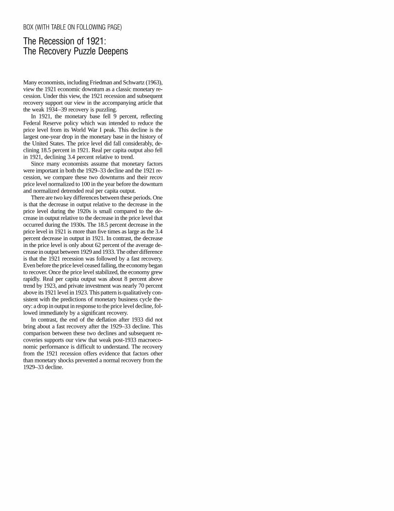
BOX (WITH TABLE ON FOLLOWING PAGE)

The Recession of 1921:The Recovery Puzzle Deepens

Many economists, including Friedman and Schwartz (1963),view the 1921 economic downturn as a classic monetary re-cession. Under this view, the 1921 recession and subsequentrecovery support our view in the accompanying article thatthe weak 1934–39 recovery is puzzling.

In 1921, the monetary base fell 9 percent, reflectingFederal Reserve policy which was intended to reduce theprice level from its World War I peak. This decline is thelargest one-year drop in the monetary base in the history ofthe United States. The price level did fall considerably, de-clining 18.5 percent in 1921. Real per capita output also fellin 1921, declining 3.4 percent relative to trend.

Since many economists assume that monetary factorswere important in both the 1929–33 decline and the 1921 re-cession, we compare these two downturns and their recovprice level normalized to 100 in the year before the downturnand normalized detrended real per capita output.

There are two key differences between these periods. Oneis that the decrease in output relative to the decrease in theprice level during the 1920s is small compared to the de-crease in output relative to the decrease in the price level thatoccurred during the 1930s. The 18.5 percent decrease in theprice level in 1921 is more than five times as large as the 3.4percent decrease in output in 1921. In contrast, the decreasein the price level is only about 62 percent of the average de-crease in output between 1929 and 1933. The other differenceis that the 1921 recession was followed by a fast recovery.Even before theprice level ceased falling, the economy beganto recover. Once the price level stabilized, the economy grewrapidly. Real per capita output was about 8 percent abovetrend by 1923, and private investment was nearly 70 percentabove its 1921 level in 1923. This pattern is qualitatively con-sistent with the predictions of monetary business cycle the-ory: a drop in output in response to the price level decline, fol-lowed immediately by a significant recovery.

In contrast, the end of the deflation after 1933 did notbring about a fast recovery after the 1929–33 decline. Thiscomparison between these two declines and subsequent re-coveries supports our view that weak post-1933 macroeco-nomic performance is difficult to understand. The recoveryfrom the 1921 recession offers evidence that factors otherthan monetary shocks prevented a normal recovery from the1929–33 decline.

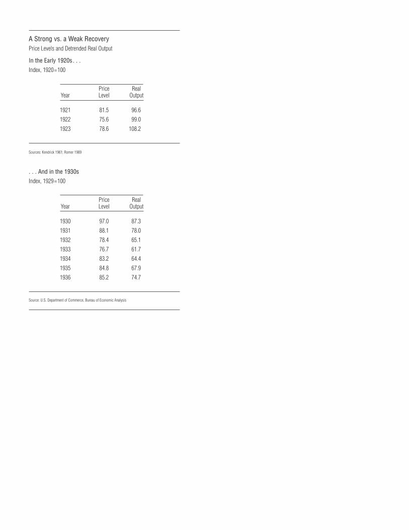
A Strong vs. a Weak RecoveryPrice Levels and Detrended Real Output

In the Early 1920s. . .

Index, 1920=100

Price RealYear Level Output

1921 81.5 96.6

1922 75.6 99.0

1923 78.6 108.2

Sources: Kendrick 1961; Romer 1989

. . . And in the 1930s

Index, 1929=100

Price RealYear Level Output

1930 97.0 87.3

1931 88.1 78.0

1932 78.4 65.1

1933 76.7 61.7

1934 83.2 64.4

1935 84.8 67.9

1936 85.2 74.7

Source: U.S. Department of Commerce, Bureau of Economic Analysis

Table 1

Duration and Scale of the Depressionand Postwar Business CyclesMeasured by the Decline and Recovery of Output

Length Size of Length ofof Decline Decline Recovery

Great Depression 4 years –31.0% 7 years

Postwar Cycle Average 1 year –2.9% 1.5 years

Sources: National Bureau of Economic Research; U.S. Department of Commerce,Bureau of Economic Analysis

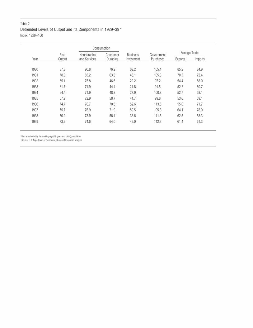
ConsumptionForeign TradeReal Nondurables Consumer Business Government

Year Output and Services Durables Investment Purchases Exports Imports

1930 87.3 90.8 76.2 69.2 105.1 85.2 84.9

1931 78.0 85.2 63.3 46.1 105.3 70.5 72.4

1932 65.1 75.8 46.6 22.2 97.2 54.4 58.0

1933 61.7 71.9 44.4 21.8 91.5 52.7 60.7

1934 64.4 71.9 48.8 27.9 100.8 52.7 58.1

1935 67.9 72.9 58.7 41.7 99.8 53.6 69.1

1936 74.7 76.7 70.5 52.6 113.5 55.0 71.7

1937 75.7 76.9 71.9 59.5 105.8 64.1 78.0

1938 70.2 73.9 56.1 38.6 111.5 62.5 58.3

1939 73.2 74.6 64.0 49.0 112.3 61.4 61.3

*Data are divided by the working-age (16 years and older) population.Source: U.S. Department of Commerce, Bureau of Economic Analysis

Table 2

Detrended Levels of Output and Its Components in 1929–39*Index, 1929=100

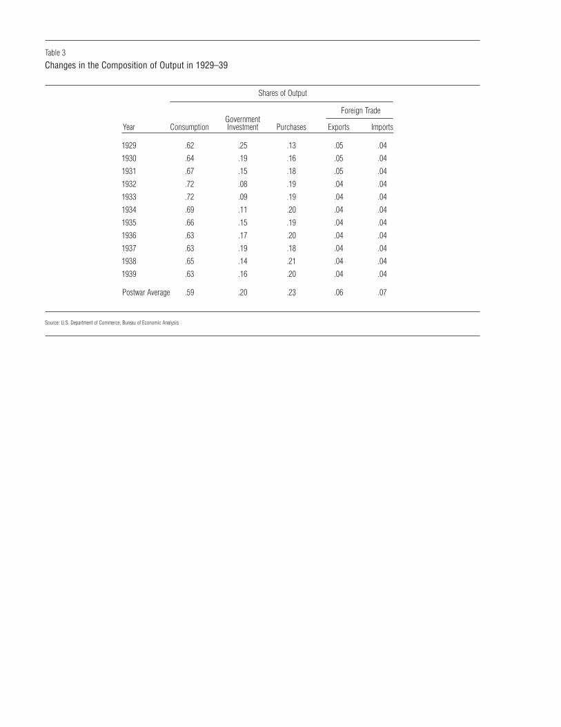
Table 3

Changes in the Composition of Output in 1929–39

GovernmentYear Consumption Investment Purchases Exports Imports

1929 .62 .25 .13 .05 .04

1930 .64 .19 .16 .05 .04

1931 .67 .15 .18 .05 .04

1932 .72 .08 .19 .04 .04

1933 .72 .09 .19 .04 .04

1934 .69 .11 .20 .04 .04

1935 .66 .15 .19 .04 .04

1936 .63 .17 .20 .04 .04

1937 .63 .19 .18 .04 .04

1938 .65 .14 .21 .04 .04

1939 .63 .16 .20 .04 .04

Postwar Average .59 .20 .23 .06 .07

Source: U.S. Department of Commerce, Bureau of Economic Analysis

Shares of Output

Foreign Trade

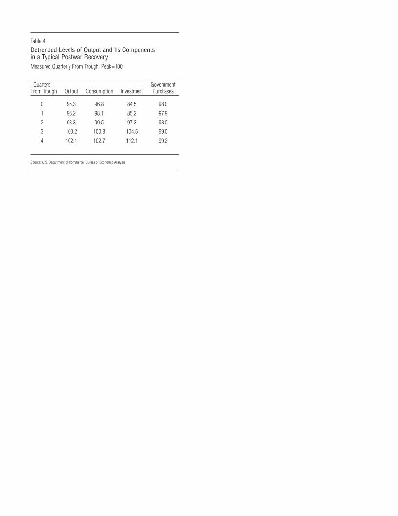
Table 4

Detrended Levels of Output and Its Componentsin a Typical Postwar RecoveryMeasured Quarterly From Trough, Peak =100

Quarters GovernmentFrom Trough Output Consumption Investment Purchases

0 95.3 96.8 84.5 98.0

1 96.2 98.1 85.2 97.9

2 98.3 99.5 97.3 98.0

3 100.2 100.8 104.5 99.0

4 102.1 102.7 112.1 99.2

Source: U.S. Department of Commerce, Bureau of Economic Analysis

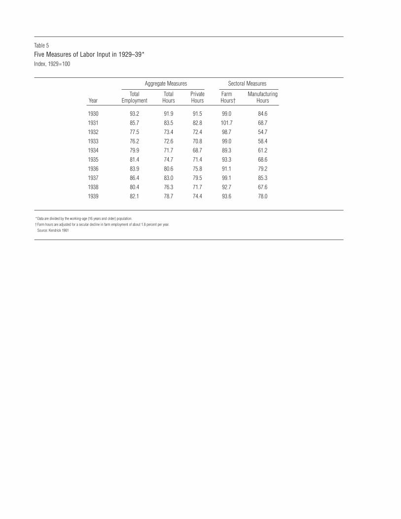
Table 5

Five Measures of Labor Input in 1929–39*Index, 1929=100

Aggregate Measures Sectoral Measures

Total Total Private Farm ManufacturingYear Employment Hours Hours Hours† Hours

1930 93.2 91.9 91.5 99.0 84.6

1931 85.7 83.5 82.8 101.7 68.7

1932 77.5 73.4 72.4 98.7 54.7

1933 76.2 72.6 70.8 99.0 58.4

1934 79.9 71.7 68.7 89.3 61.2

1935 81.4 74.7 71.4 93.3 68.6

1936 83.9 80.6 75.8 91.1 79.2

1937 86.4 83.0 79.5 99.1 85.3

1938 80.4 76.3 71.7 92.7 67.6

1939 82.1 78.7 74.4 93.6 78.0

*Data are divided by the working-age (16 years and older) population.† Farm hours are adjusted for a secular decline in farm employment of about 1.8 percent per year.

Source: Kendrick 1961

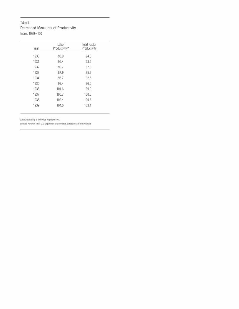
Table 6

Detrended Measures of ProductivityIndex, 1929 = 100

Labor Total FactorYear Productivity* Productivity

1930 95.9 94.8

1931 95.4 93.5

1932 90.7 87.8

1933 87.9 85.9

1934 96.7 92.6

1935 98.4 96.6

1936 101.6 99.9

1937 100.7 100.5

1938 102.4 100.3

1939 104.6 103.1

*Labor productivity is defined as output per hour.

Sources: Kendrick 1961; U.S. Department of Commerce, Bureau of Economic Analysis

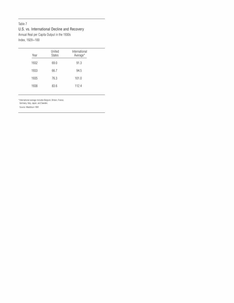
Table 7

U.S. vs. International Decline and RecoveryAnnual Real per Capita Output in the 1930s

Index, 1929 =100

United InternationalYear States Average*

1932 69.0 91.3

1933 66.7 94.5

1935 76.3 101.0

1938 83.6 112.4

* International average includes Belgium, Britain, France,Germany, Italy, Japan, and Sweden.

Source: Maddison 1991

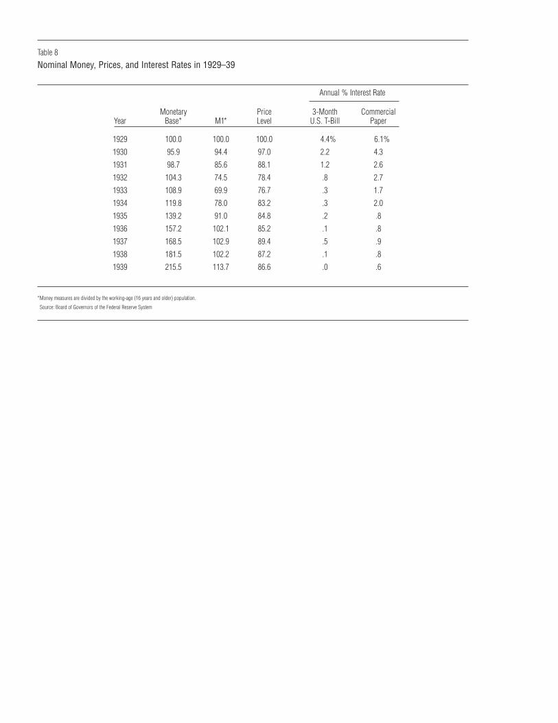
Table 8

Nominal Money, Prices, and Interest Rates in 1929–39

Annual % Interest Rate

Monetary Price 3-Month CommercialYear Base* M1* Level U.S. T-Bill Paper

1929 100.0 100.0 100.0 4.4% 6.1%

1930 95.9 94.4 97.0 2.2 4.3

1931 98.7 85.6 88.1 1.2 2.6

1932 104.3 74.5 78.4 .8 2.7

1933 108.9 69.9 76.7 .3 1.7

1934 119.8 78.0 83.2 .3 2.0

1935 139.2 91.0 84.8 .2 .8

1936 157.2 102.1 85.2 .1 .8

1937 168.5 102.9 89.4 .5 .9

1938 181.5 102.2 87.2 .1 .8

1939 215.5 113.7 86.6 .0 .6

*Money measures are divided by the working-age (16 years and older) population.

Source: Board of Governors of the Federal Reserve System

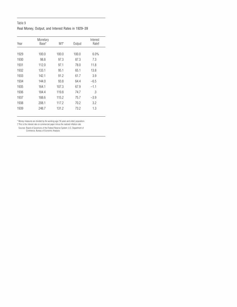
Table 9

Real Money, Output, and Interest Rates in 1929–39

Monetary InterestYear Base* M1* Output Rate†

1929 100.0 100.0 100.0 6.0%

1930 98.8 97.3 87.3 7.3

1931 112.0 97.1 78.0 11.8

1932 133.1 95.1 65.1 13.8

1933 142.1 91.2 61.7 3.9

1934 144.0 93.8 64.4 –6.5

1935 164.1 107.3 67.9 –1.1

1936 184.4 119.8 74.7 .3

1937 188.6 115.2 75.7 –3.9

1938 208.1 117.2 70.2 3.2

1939 248.7 131.2 73.2 1.3

* Money measures are divided by the working-age (16 years and older) population.† This is the interest rate on commercial paper minus the realized inflation rate.

Sources: Board of Governors of the Federal Reserve System; U.S. Department ofCommerce, Bureau of Economic Analysis

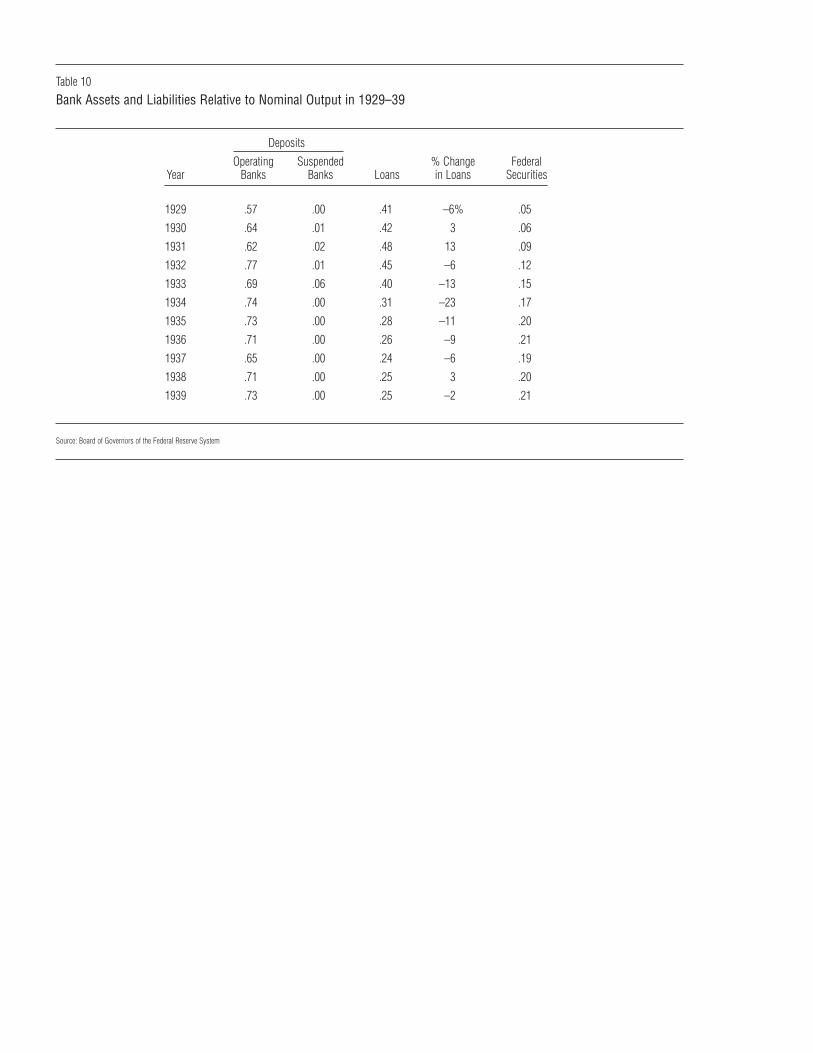
Table 10

Bank Assets and Liabilities Relative to Nominal Output in 1929–39

Deposits

Operating Suspended % Change FederalYear Banks Banks Loans in Loans Securities

1929 .57 .00 .41 –6% .05

1930 .64 .01 .42 3 .06

1931 .62 .02 .48 13 .09

1932 .77 .01 .45 –6 .12

1933 .69 .06 .40 –13 .15

1934 .74 .00 .31 –23 .17

1935 .73 .00 .28 –11 .20

1936 .71 .00 .26 –9 .21

1937 .65 .00 .24 –6 .19

1938 .71 .00 .25 3 .20

1939 .73 .00 .25 –2 .21

Source: Board of Governors of the Federal Reserve System

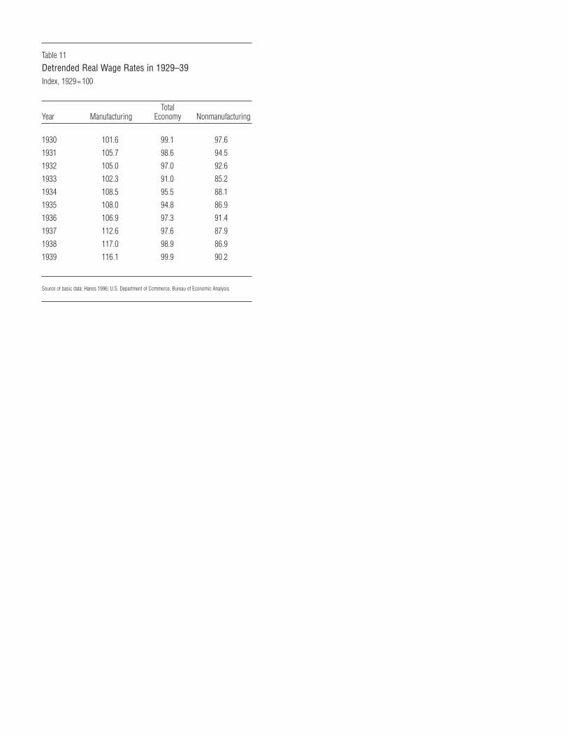
Table 11

Detrended Real Wage Rates in 1929–39Index, 1929= 100

TotalYear Manufacturing Economy Nonmanufacturing

1930 101.6 99.1 97.6

1931 105.7 98.6 94.5

1932 105.0 97.0 92.6

1933 102.3 91.0 85.2

1934 108.5 95.5 88.1

1935 108.0 94.8 86.9

1936 106.9 97.3 91.4

1937 112.6 97.6 87.9

1938 117.0 98.9 86.9

1939 116.1 99.9 90.2

Source of basic data: Hanes 1996; U.S. Department of Commerce, Bureau of Economic Analysis

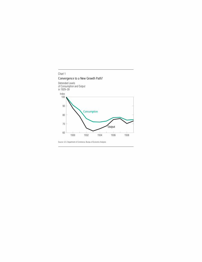
Consumption

Output

Chart 1

Convergence to a New Growth Path?Detrended Levelsof Consumption and Outputin 1929–39

Source: U.S. Department of Commerce, Bureau of Economic Analysis

1930 1932 1934 1936 193860

70

80

90

Index100

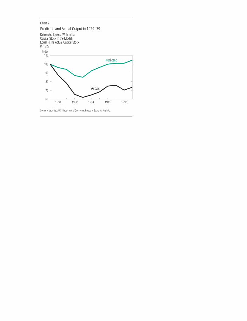
Chart 2

Predicted and Actual Output in 1929–39Detrended Levels, With InitialCapital Stock in the ModelEqual to the Actual Capital Stockin 1929

Source of basic data: U.S. Department of Commerce, Bureau of Economic Analysis

1930 1932 1934 1936 193860

70

80

90

100

Index110

Predicted

Actual

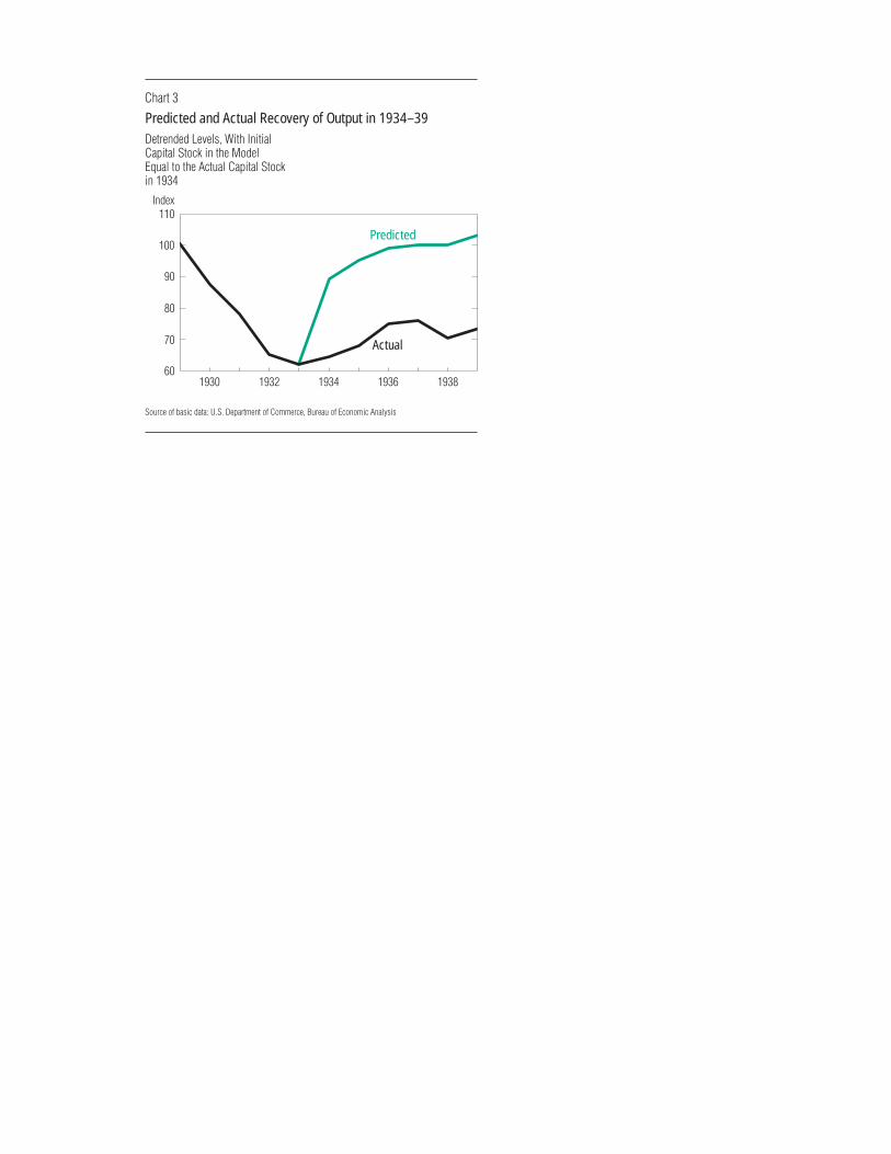
Predicted

Actual

Chart 3

Predicted and Actual Recovery of Output in 1934–39Detrended Levels, With InitialCapital Stock in the ModelEqual to the Actual Capital Stock in 1934

Source of basic data: U.S. Department of Commerce, Bureau of Economic Analysis

1930 1932 1934 1936 193860

70

80

90

100

Index110