The gravitational self-force

[E. Poisson, Living Reviews in Relativity 7, 6 (2004); gr-qc/0306052]

1. Capra scientific mandate

2. Introduction

3. Motion of a black hole

4. Motion of a point mass

5. Newtonian self-force

6. Multipole decomposition of the self-force

7. Beyond the self-force

8. Conclusion

1

1. Capra scientific mandate

To formulate the equations of motion of a small body of mass m in

a specified background spacetime, beyond the test-mass

approximation.

This first step was solved back in 1997. The equations of motion are now known as

the MiSaTaQuWa equations. I will sketch a derivation of these equations.

To concretely describe this motion for situations of astrophysical

interest (generic orbits of a Kerr black hole).

Much recent progress on this front. I will describe some of the issues involved.

To properly incorporate this information into a wave-generation

formalism.

The holy grail: still elusive. I will present a tentative outline of future work.

2

The work reviewed in this talk was shaped by a series of seven

“Capra” meetings, from 1998 to 2004:

Capra Ranch, Dublin, Pasadena, Potsdam, State College PA, Kyoto, and

Brownsville.

Members of the Capra posse include:

Paul Anderson, Warren Anderson, Leor Barack, Patrick Brady, Lior Burko,

Manuella Campanelli, Steve Detweiler, Eanna Flanagan, Costas Glempedakis,

Abraham Harte, Wataru Hikida, Bei Lok Hu, Scott Hughes, Sanjay Jhingan,

Dong-Hoon Kim, Carlos Lousto, Eirini Messaritaki, Yasushi Mino, Hiroyuki Nakano,

Amos Ori, Eric Poisson, Ted Quinn, Eran Rosenthal, Norichika Sago, Misao Sasaki,

Takahiro Tanaka, Bob Wald, Bernard Whiting, and Alan Wiseman.

3

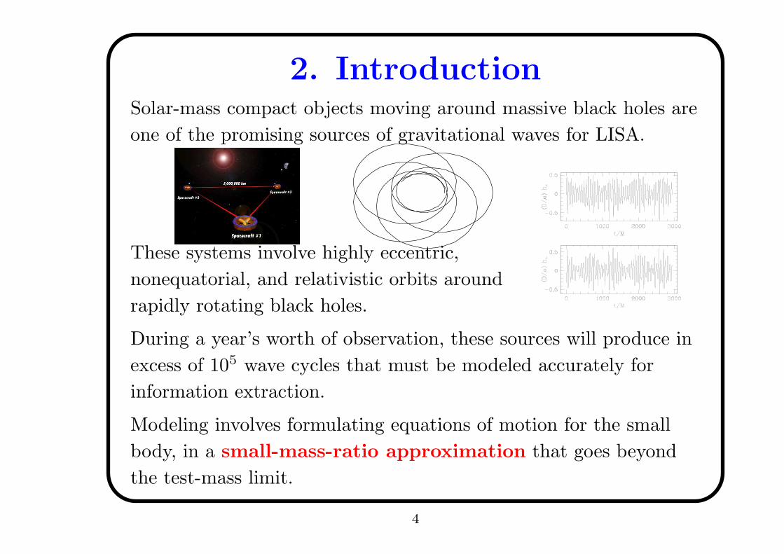
2. IntroductionSolar-mass compact objects moving around massive black holes are

one of the promising sources of gravitational waves for LISA.

These systems involve highly eccentric,

nonequatorial, and relativistic orbits around

rapidly rotating black holes.

During a year’s worth of observation, these sources will produce in

excess of 105 wave cycles that must be modeled accurately for

information extraction.

Modeling involves formulating equations of motion for the small

body, in a small-mass-ratio approximation that goes beyond

the test-mass limit.

4

Corrections to the equations of motion must incorporate

• conservative effects, such as periastron advance

(which can lead to a large cumulative dephasing);

• dissipative effects, such as loss of orbital energy and angular

momentum to gravitational radiation

(which produces a frequency sweep in the LISA band).

Modeling also involves improving the wave-generation calculations

to consistently incorporate

• the corrected equations of motion;

• the effect of the small body’s gravitational field on wave

generation and propagation.

5

3. Motion of a black hole

A body of mass m moves in an arbitrary (but empty) spacetime

whose radius of curvature (in a neighbourhood of the body) is R;

we assume that m/R 1.

When viewed on a large scale R, the body appears to move on a

world line γ described by parametric relations zµ(τ); we wish to

determine this world line.

A compelling way to proceed is to assume that the body is a

nonrotating black hole [Mino, Sasaki, and Tanaka (1997)].

The metric of the black hole perturbed by the tidal gravitational

field of the external universe is matched to the metric of the

background spacetime perturbed by the moving black hole.

6

Demanding that this metric be a solution to the vacuum field

equation determines the motion of the black hole.

The method of matched asymptotic expansions relies on the

existence of

• an internal zone in which r/R 1, where r is the distance to

the black hole (here gravity is dominated by the black hole);

• an external zone in which m/r 1 (here gravity is

dominated by the external universe);

• a buffer zone in which r/R and m/r are both small (here the

black hole and the external universe have comparable gravities).

The metrics are matched in the buffer zone, where m r R.

7

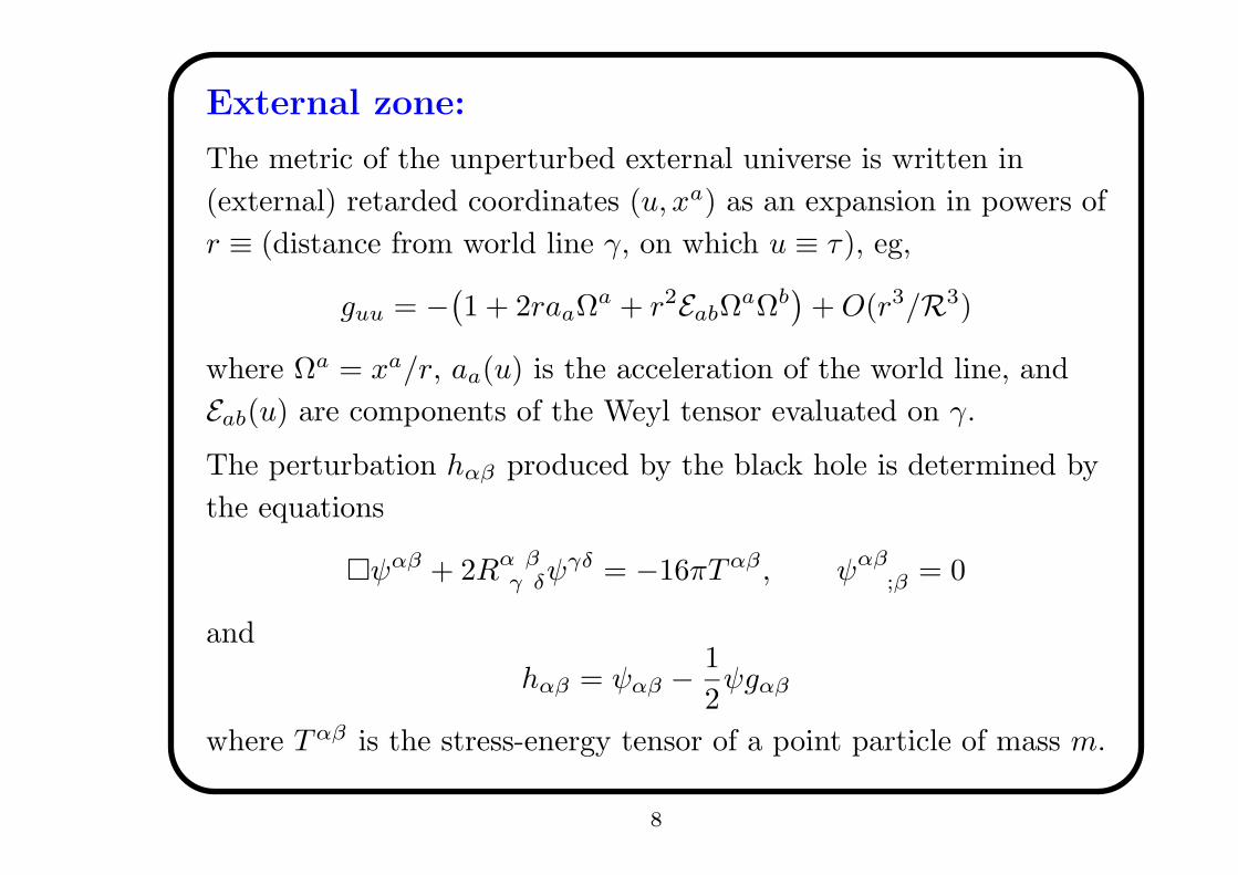
External zone:

The metric of the unperturbed external universe is written in

(external) retarded coordinates (u, xa) as an expansion in powers of

r ≡ (distance from world line γ, on which u ≡ τ), eg,

guu = −(1 + 2raaΩa + r2EabΩ

aΩb)

+O(r3/R3)

where Ωa = xa/r, aa(u) is the acceleration of the world line, and

Eab(u) are components of the Weyl tensor evaluated on γ.

The perturbation hαβ produced by the black hole is determined by

the equations

ψαβ + 2Rα βγ δψ

γδ = −16πTαβ , ψαβ;β = 0

and

hαβ = ψαβ −1

2ψgαβ

where Tαβ is the stress-energy tensor of a point particle of mass m.

8

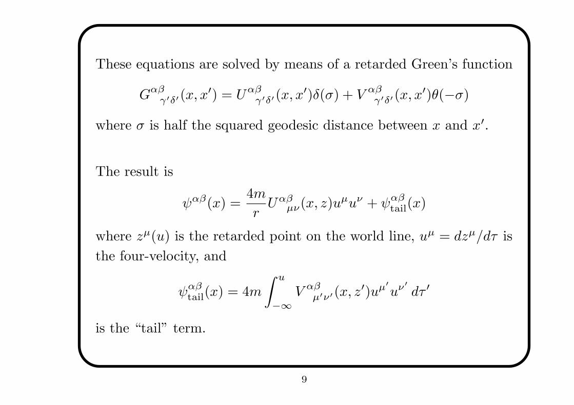
These equations are solved by means of a retarded Green’s function

Gαβγ′δ′(x, x

′) = Uαβγ′δ′(x, x

′)δ(σ) + V αβγ′δ′(x, x

′)θ(−σ)

where σ is half the squared geodesic distance between x and x′.

The result is

ψαβ(x) =4m

rUαβ

µν(x, z)uµuν + ψαβtail(x)

where zµ(u) is the retarded point on the world line, uµ = dzµ/dτ is

the four-velocity, and

ψαβtail(x) = 4m

∫ u

−∞

V αβµ′ν′(x, z

′)uµ′

uν′

dτ ′

is the “tail” term.

9

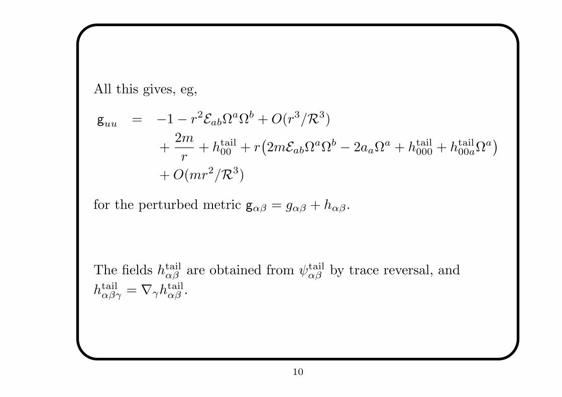
All this gives, eg,

guu = −1 − r2EabΩaΩb +O(r3/R3)

+2m

r+ htail

00 + r(2mEabΩ

aΩb − 2aaΩa + htail000 + htail

00aΩa)

+O(mr2/R3)

for the perturbed metric gαβ = gαβ + hαβ .

The fields htailαβ are obtained from ψtail

αβ by trace reversal, and

htailαβγ = ∇γh

tailαβ .

10

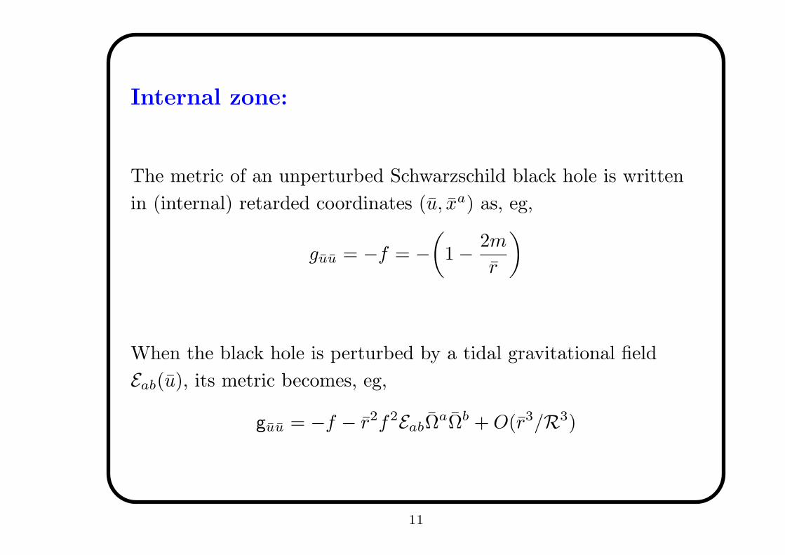
Internal zone:

The metric of an unperturbed Schwarzschild black hole is written

in (internal) retarded coordinates (u, xa) as, eg,

guu = −f = −

(

1 −2m

r

)

When the black hole is perturbed by a tidal gravitational field

Eab(u), its metric becomes, eg,

guu = −f − r2f2EabΩaΩb +O(r3/R3)

11

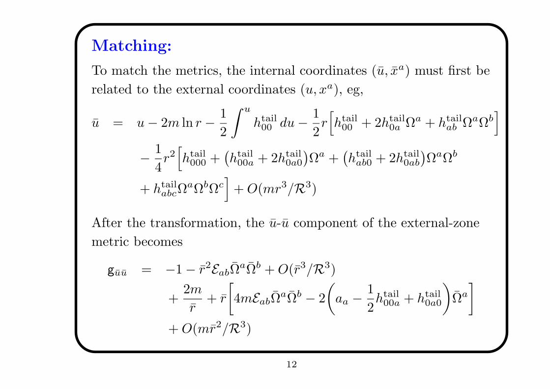
Matching:

To match the metrics, the internal coordinates (u, xa) must first be

related to the external coordinates (u, xa), eg,

u = u− 2m ln r −1

2

∫ u

htail00 du−

1

2r[

htail00 + 2htail

0a Ωa + htailab ΩaΩb

]

−1

4r2

[

htail000 +

(htail

00a + 2htail0a0

)Ωa +

(htail

ab0 + 2htail0ab

)ΩaΩb

+ htailabcΩ

aΩbΩc]

+O(mr3/R3)

After the transformation, the u-u component of the external-zone

metric becomes

guu = −1 − r2EabΩaΩb +O(r3/R3)

+2m

r+ r

[

4mEabΩaΩb − 2

(

aa −1

2htail

00a + htail0a0

)

Ωa

]

+O(mr2/R3)

12

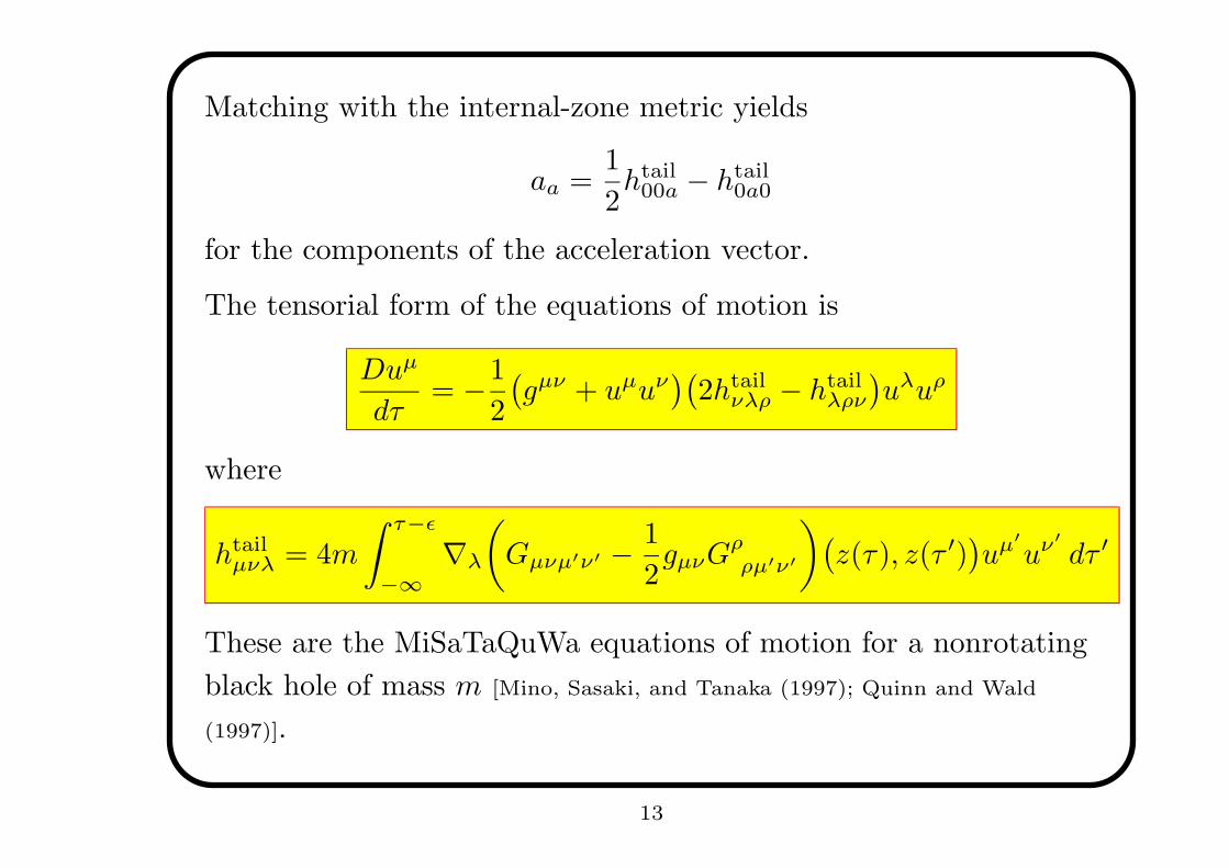
Matching with the internal-zone metric yields

aa =1

2htail

00a − htail0a0

for the components of the acceleration vector.

The tensorial form of the equations of motion is

Duµ

dτ= −

1

2

(gµν + uµuν

)(2htail

νλρ − htailλρν

)uλuρ

where

htailµνλ = 4m

∫ τ−ε

−∞

∇λ

(

Gµνµ′ν′ −1

2gµνG

ρρµ′ν′

)(z(τ), z(τ ′)

)uµ′

uν′

dτ ′

These are the MiSaTaQuWa equations of motion for a nonrotating

black hole of mass m [Mino, Sasaki, and Tanaka (1997); Quinn and Wald

(1997)].

13

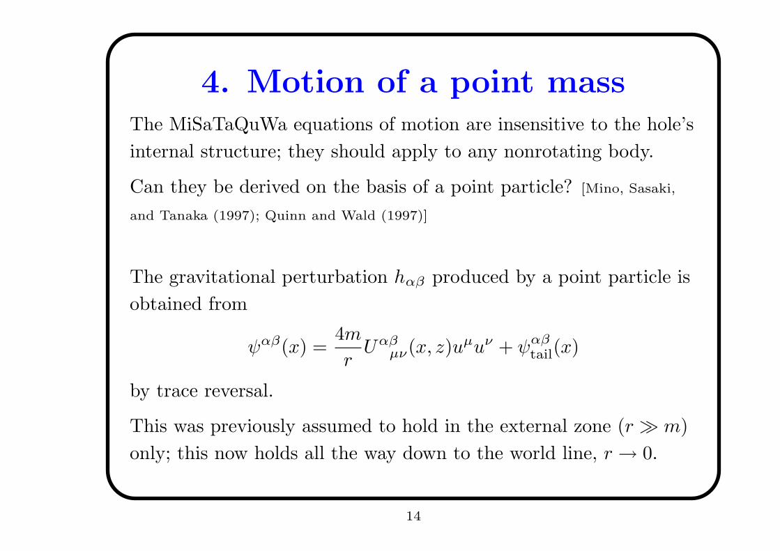
4. Motion of a point mass

The MiSaTaQuWa equations of motion are insensitive to the hole’s

internal structure; they should apply to any nonrotating body.

Can they be derived on the basis of a point particle? [Mino, Sasaki,

and Tanaka (1997); Quinn and Wald (1997)]

The gravitational perturbation hαβ produced by a point particle is

obtained from

ψαβ(x) =4m

rUαβ

µν(x, z)uµuν + ψαβtail(x)

by trace reversal.

This was previously assumed to hold in the external zone (r m)

only; this now holds all the way down to the world line, r → 0.

14

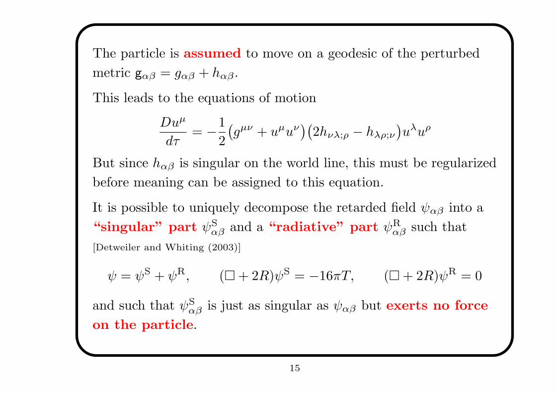
The particle is assumed to move on a geodesic of the perturbed

metric gαβ = gαβ + hαβ .

This leads to the equations of motion

Duµ

dτ= −

1

2

(gµν + uµuν

)(2hνλ;ρ − hλρ;ν

)uλuρ

But since hαβ is singular on the world line, this must be regularized

before meaning can be assigned to this equation.

It is possible to uniquely decompose the retarded field ψαβ into a

“singular” part ψSαβ and a “radiative” part ψR

αβ such that

[Detweiler and Whiting (2003)]

ψ = ψS + ψR, ( + 2R)ψS = −16πT, ( + 2R)ψR = 0

and such that ψSαβ is just as singular as ψαβ but exerts no force

on the particle.

15

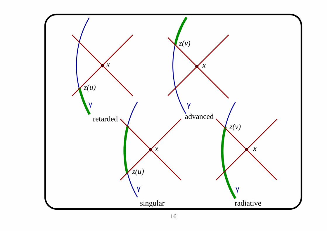
γ

x

z(u)

retarded

z(v)

x

γadvanced

γ

x

z(u)

singular

x

γ

z(v)

radiative

16

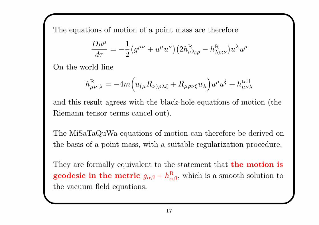
The equations of motion of a point mass are therefore

Duµ

dτ= −

1

2

(gµν + uµuν

)(2hR

νλ;ρ − hRλρ;ν

)uλuρ

On the world line

hRµν;λ = −4m

(

u(µRν)ρλξ +Rµρνξuλ

)

uρuξ + htailµνλ

and this result agrees with the black-hole equations of motion (the

Riemann tensor terms cancel out).

The MiSaTaQuWa equations of motion can therefore be derived on

the basis of a point mass, with a suitable regularization procedure.

They are formally equivalent to the statement that the motion is

geodesic in the metric gαβ + hRαβ , which is a smooth solution to

the vacuum field equations.

17

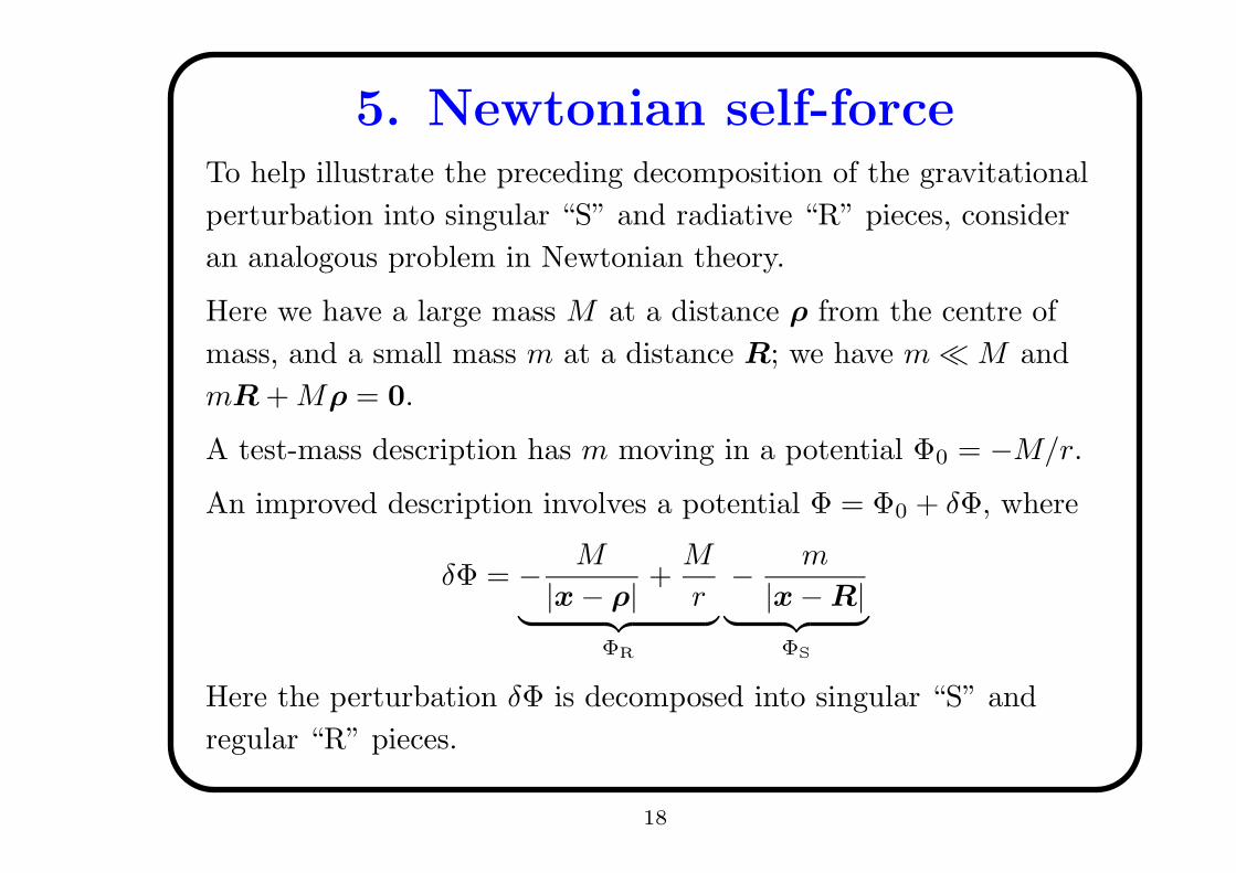
5. Newtonian self-forceTo help illustrate the preceding decomposition of the gravitational

perturbation into singular “S” and radiative “R” pieces, consider

an analogous problem in Newtonian theory.

Here we have a large mass M at a distance ρ from the centre of

mass, and a small mass m at a distance R; we have mM and

mR +Mρ = 0.

A test-mass description has m moving in a potential Φ0 = −M/r.

An improved description involves a potential Φ = Φ0 + δΦ, where

δΦ = −M

|x − ρ|+M

r︸ ︷︷ ︸

ΦR

−m

|x − R|︸ ︷︷ ︸

ΦS

Here the perturbation δΦ is decomposed into singular “S” and

regular “R” pieces.

18

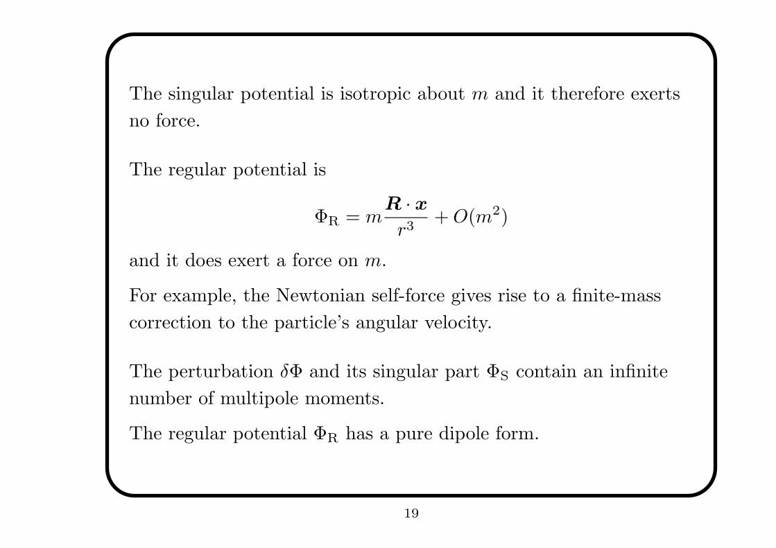
The singular potential is isotropic about m and it therefore exerts

no force.

The regular potential is

ΦR = mR · x

r3+O(m2)

and it does exert a force on m.

For example, the Newtonian self-force gives rise to a finite-mass

correction to the particle’s angular velocity.

The perturbation δΦ and its singular part ΦS contain an infinite

number of multipole moments.

The regular potential ΦR has a pure dipole form.

19

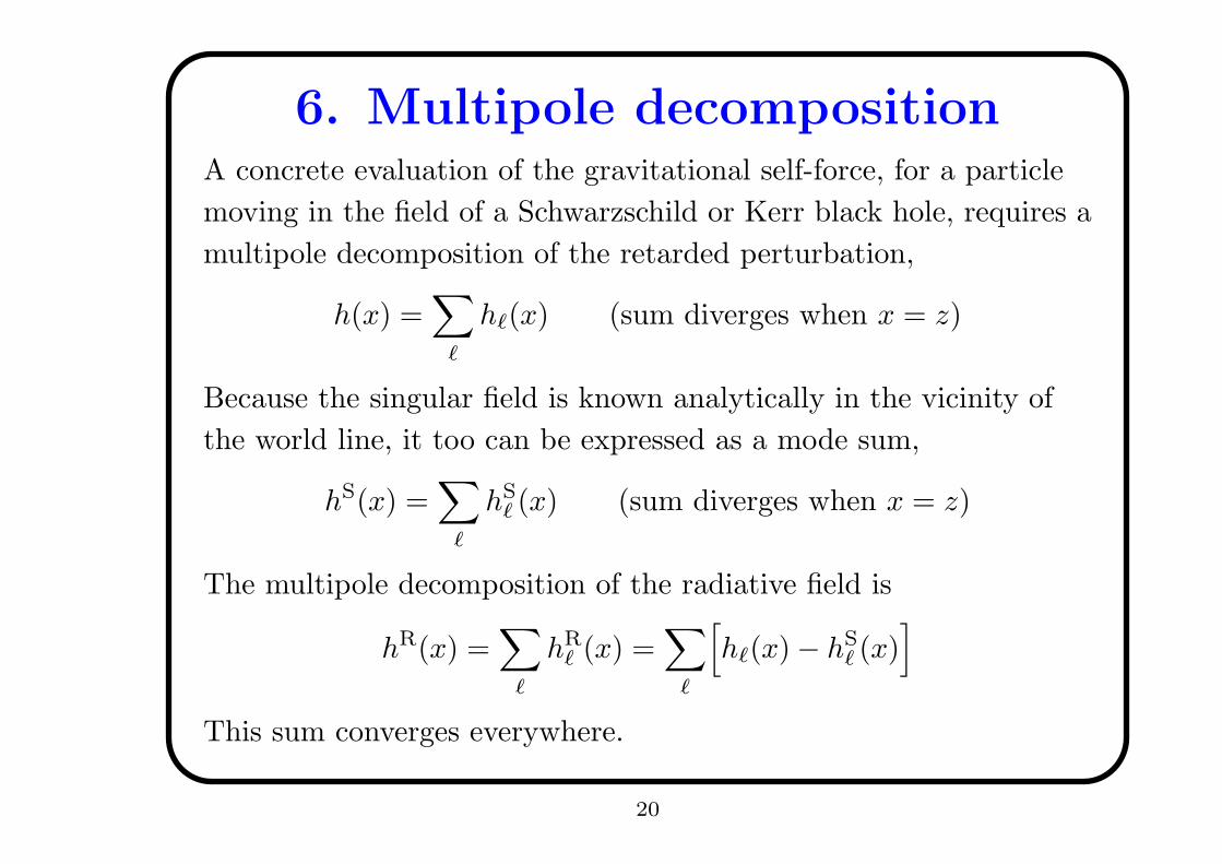
6. Multipole decompositionA concrete evaluation of the gravitational self-force, for a particle

moving in the field of a Schwarzschild or Kerr black hole, requires a

multipole decomposition of the retarded perturbation,

h(x) =∑

`

h`(x) (sum diverges when x = z)

Because the singular field is known analytically in the vicinity of

the world line, it too can be expressed as a mode sum,

hS(x) =∑

`

hS` (x) (sum diverges when x = z)

The multipole decomposition of the radiative field is

hR(x) =∑

`

hR` (x) =

∑

`

[

h`(x) − hS` (x)

]

This sum converges everywhere.

20

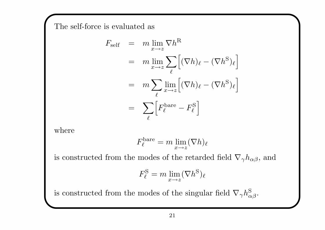
The self-force is evaluated as

Fself = m limx→z

∇hR

= m limx→z

∑

`

[

(∇h)` − (∇hS)`

]

= m∑

`

limx→z

[

(∇h)` − (∇hS)`

]

=∑

`

[

F bare` − F S

`

]

where

F bare` = m lim

x→z(∇h)`

is constructed from the modes of the retarded field ∇γhαβ , and

F S` = m lim

x→z(∇hS)`

is constructed from the modes of the singular field ∇γhSαβ .

21

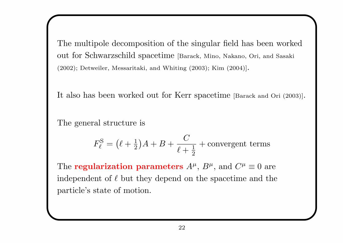
The multipole decomposition of the singular field has been worked

out for Schwarzschild spacetime [Barack, Mino, Nakano, Ori, and Sasaki

(2002); Detweiler, Messaritaki, and Whiting (2003); Kim (2004)].

It also has been worked out for Kerr spacetime [Barack and Ori (2003)].

The general structure is

F S` =

(`+ 1

2

)A+B +

C

`+ 12

+ convergent terms

The regularization parameters Aµ, Bµ, and Cµ ≡ 0 are

independent of ` but they depend on the spacetime and the

particle’s state of motion.

22

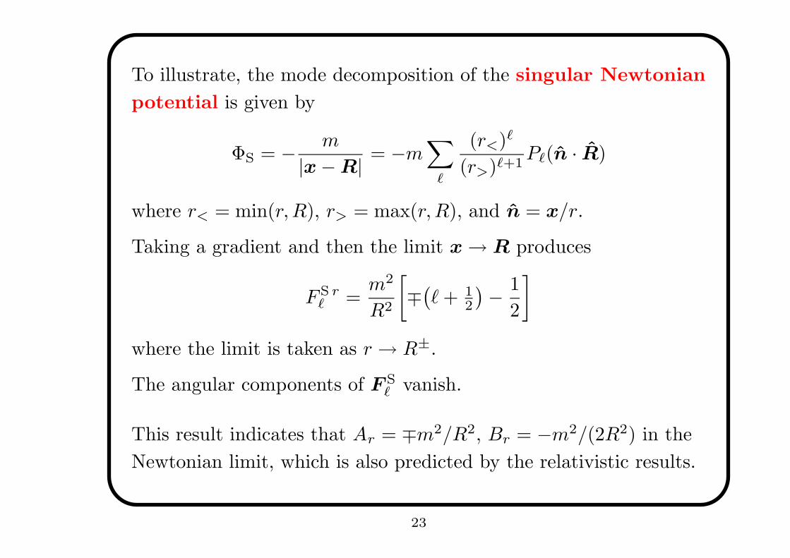
To illustrate, the mode decomposition of the singular Newtonian

potential is given by

ΦS = −m

|x − R|= −m

∑

`

(r<)`

(r>)`+1P`(n · R)

where r< = min(r,R), r> = max(r,R), and n = x/r.

Taking a gradient and then the limit x → R produces

F S r` =

m2

R2

[

∓(`+ 1

2

)−

1

2

]

where the limit is taken as r → R±.

The angular components of F S` vanish.

This result indicates that Ar = ∓m2/R2, Br = −m2/(2R2) in the

Newtonian limit, which is also predicted by the relativistic results.

23

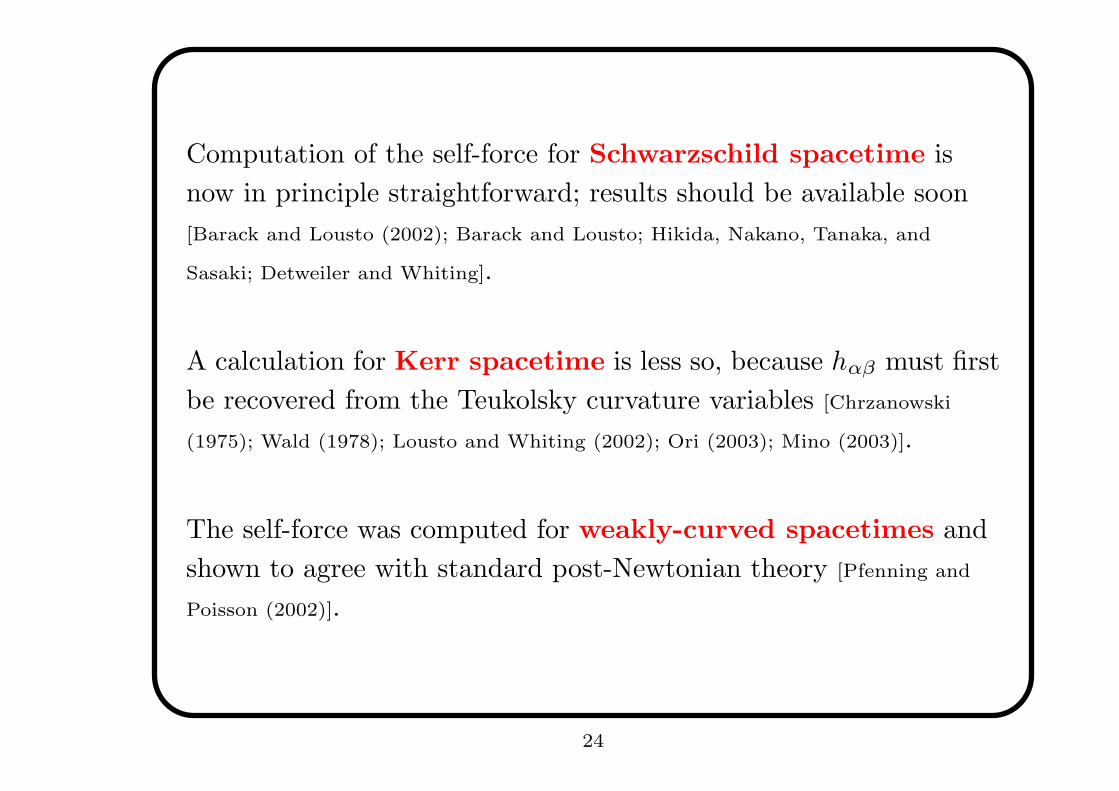
Computation of the self-force for Schwarzschild spacetime is

now in principle straightforward; results should be available soon

[Barack and Lousto (2002); Barack and Lousto; Hikida, Nakano, Tanaka, and

Sasaki; Detweiler and Whiting].

A calculation for Kerr spacetime is less so, because hαβ must first

be recovered from the Teukolsky curvature variables [Chrzanowski

(1975); Wald (1978); Lousto and Whiting (2002); Ori (2003); Mino (2003)].

The self-force was computed for weakly-curved spacetimes and

shown to agree with standard post-Newtonian theory [Pfenning and

Poisson (2002)].

24

7. Beyond the self-force

The gravitational self-force is not gauge invariant — it is

formulated in the Lorenz gauge ψαβ;β = 0 — and it must be

combined with other inputs to extract observational consequences.

For example, if the particle is a pulsar, then the self-force and the

perturbed metric gαβ = gαβ + hαβ can be used together to

calculate the pulses’ times-of-arrival.

Ultimately we want gravitational waveforms, and this requires

inputs from second-order perturbation theory.

25

Consider the first-order problem:

( + 2R)h1 = −16πT [z]

Consistency demands that z(τ) be a geodesic of the background

spacetime, and the waveforms obtained from h1 do not incorporate

self-force information.

Consider next the second-order problem:

( + 2R)h2 = −16π(1 + h1)T [z + δz] + (∇h1)2

where δz(τ) is the correction to the geodesic motion.

The waveforms obtained from h2 properly incorporate self-force

information, in a gauge-invariant manner.

Getting waveforms therefore requires (defining and) solving the

second-order problem [Ori and Rosenthal].

26

7. Conclusion

There has been significant progress in the self-force problem over

the last several years:

• the foundations are solid;

• the regularization parameters Aµ, Bµ, and Cµ are known for

arbitrary motion in Schwarzschild and Kerr spacetimes;

• metric reconstruction from the Teukolsky curvature variables is

better understood.

27

But there are difficult outstanding issues:

• how to define and calculate the low-multipole (` = 0 and ` = 1)

contributions to the self-force in Kerr?

• what useful gauge-invariant quantities can be computed from

the self-force and the metric perturbation?

• how to properly incorporate the self-force into a

wave-generation formalism?

28