The graph neural network model - Persagen Consulting · In this paper, we present a supervised neural network model, which is suitable for both graph and node-focused applications

University of WollongongResearch Online

Faculty of Informatics - Papers (Archive) Faculty of Engineering and Information Sciences

2009

The graph neural network modelFranco ScarselliUniversity of Siena

Marco GoriUniversity of Siena

Ah Chung TsoiHong Kong Baptist University, [email protected]

Markus HagenbuchnerUniversity of Wollongong, [email protected]

Gabriele MonfardiniUniversity of Siena

Research Online is the open access institutional repository for the University of Wollongong. For further information contact the UOW Library:[email protected]

Publication DetailsScarselli, F., Gori, M., Tsoi, A., Hagenbuchner, M. & Monfardini, G. 2009, 'The graph neural network model', IEEE Transactions onNeural Networks, vol. 20, no. 1, pp. 61-80.

http://ro.uow.edu.au/



http://ro.uow.edu.au

http://ro.uow.edu.au/infopapers

http://ro.uow.edu.au/eis

The graph neural network model

AbstractMany underlying relationships among data in several areas of science and engineering, e.g., computer vision,molecular chemistry, molecular biology, pattern recognition, and data mining, can be represented in terms ofgraphs. In this paper, we propose a new neural network model, called graph neural network (GNN) model,that extends existing neural network methods for processing the data represented in graph domains. ThisGNN model, which can directly process most of the practically useful types of graphs, e.g., acyclic, cyclic,directed, and undirected, implements a function tau(G,n) isin IRm that maps a graph G and one of its nodes ninto an m-dimensional Euclidean space. A supervised learning algorithm is derived to estimate the parametersof the proposed GNN model. The computational cost of the proposed algorithm is also considered. Someexperimental results are shown to validate the proposed learning algorithm, and to demonstrate itsgeneralization capabilities.

DisciplinesPhysical Sciences and Mathematics

Publication DetailsScarselli, F., Gori, M., Tsoi, A., Hagenbuchner, M. & Monfardini, G. 2009, 'The graph neural network model',IEEE Transactions on Neural Networks, vol. 20, no. 1, pp. 61-80.

This journal article is available at Research Online: http://ro.uow.edu.au/infopapers/3165

http://ro.uow.edu.au/infopapers/3165

IEEE TRANSACTIONS ON NEURAL NETWORKS, VOL. 20, NO. 1, JANUARY 2009 61

The Graph Neural Network ModelFranco Scarselli, Marco Gori, Fellow, IEEE, Ah Chung Tsoi, Markus Hagenbuchner, Member, IEEE, and

Gabriele Monfardini

Abstract—Many underlying relationships among data in severalareas of science and engineering, e.g., computer vision, molec-ular chemistry, molecular biology, pattern recognition, and datamining, can be represented in terms of graphs. In this paper, wepropose a new neural network model, called graph neural network(GNN) model, that extends existing neural network methods forprocessing the data represented in graph domains. This GNNmodel, which can directly process most of the practically usefultypes of graphs, e.g., acyclic, cyclic, directed, and undirected,implements a function � � that maps a graphand one of its nodes into an -dimensional Euclidean space. Asupervised learning algorithm is derived to estimate the param-eters of the proposed GNN model. The computational cost of theproposed algorithm is also considered. Some experimental resultsare shown to validate the proposed learning algorithm, and todemonstrate its generalization capabilities.

Index Terms—Graphical domains, graph neural networks(GNNs), graph processing, recursive neural networks.

I. INTRODUCTION

D ATA can be naturally represented by graph structures inseveral application areas, including proteomics [1], image

analysis [2], scene description [3], [4], software engineering [5],[6], and natural language processing [7]. The simplest kinds ofgraph structures include single nodes and sequences. But in sev-eral applications, the information is organized in more complexgraph structures such as trees, acyclic graphs, or cyclic graphs.Traditionally, data relationships exploitation has been the sub-ject of many studies in the community of inductive logic pro-gramming and, recently, this research theme has been evolvingin different directions [8], also because of the applications ofrelevant concepts in statistics and neural networks to such areas(see, for example, the recent workshops [9]–[12]).

In machine learning, structured data is often associated withthe goal of (supervised or unsupervised) learning from exam-

Manuscript received May 24, 2007; revised January 08, 2008 and May 02,2008; accepted June 15, 2008. First published December 09, 2008; current ver-sion published January 05, 2009. This work was supported by the AustralianResearch Council in the form of an International Research Exchange schemewhich facilitated the visit by F. Scarselli to University of Wollongong when theinitial work on this paper was performed. This work was also supported by theARC Linkage International Grant LX045446 and the ARC Discovery ProjectGrant DP0453089.

F. Scarselli, M. Gori, and G. Monfardini are with the Faculty of Informa-tion Engineering, University of Siena, Siena 53100, Italy (e-mail: [email protected]; [email protected]; [email protected]).

A. C. Tsoi is with Hong Kong Baptist University, Kowloon, Hong Kong(e-mail: [email protected]).

M. Hagenbuchner is with the University of Wollongong, Wollongong, N.S.W.2522, Australia (e-mail: [email protected]).

Color versions of one or more of the figures in this paper are available onlineat http://ieeexplore.ieee.org.

Digital Object Identifier 10.1109/TNN.2008.2005605

ples a function that maps a graph and one of its nodes toa vector of reals1: . Applications to a graphicaldomain can generally be divided into two broad classes, calledgraph-focused and node-focused applications, respectively, inthis paper. In graph-focused applications, the function is in-dependent of the node and implements a classifier or a re-gressor on a graph structured data set. For example, a chemicalcompound can be modeled by a graph , the nodes of whichstand for atoms (or chemical groups) and the edges of whichrepresent chemical bonds [see Fig. 1(a)] linking together someof the atoms. The mapping may be used to estimate theprobability that the chemical compound causes a certain disease[13]. In Fig. 1(b), an image is represented by a region adjacencygraph where nodes denote homogeneous regions of intensity ofthe image and arcs represent their adjacency relationship [14]. Inthis case, may be used to classify the image into differentclasses according to its contents, e.g., castles, cars, people, andso on.

In node-focused applications, depends on the node , sothat the classification (or the regression) depends on the proper-ties of each node. Object detection is an example of this class ofapplications. It consists of finding whether an image contains agiven object, and, if so, localizing its position [15]. This problemcan be solved by a function , which classifies the nodes of theregion adjacency graph according to whether the correspondingregion belongs to the object. For example, the output of forFig. 1(b) might be 1 for black nodes, which correspond to thecastle, and 0 otherwise. Another example comes from web pageclassification. The web can be represented by a graph wherenodes stand for pages and edges represent the hyperlinks be-tween them [Fig. 1(c)]. The web connectivity can be exploited,along with page contents, for several purposes, e.g., classifyingthe pages into a set of topics.

Traditional machine learning applications cope with graphstructured data by using a preprocessing phase which maps thegraph structured information to a simpler representation, e.g.,vectors of reals [16]. In other words, the preprocessing step first“squashes” the graph structured data into a vector of reals andthen deals with the preprocessed data using a list-based dataprocessing technique. However, important information, e.g., thetopological dependency of information on each node may belost during the preprocessing stage and the final result may de-pend, in an unpredictable manner, on the details of the prepro-cessing algorithm. More recently, there have been various ap-proaches [17], [18] attempting to preserve the graph structurednature of the data for as long as required before the processing

1Note that in most classification problems, the mapping is to a vector of inte-gers �� , while in regression problems, the mapping is to a vector of reals �� .Here, for simplicity of exposition, we will denote only the regression case. Theproposed formulation can be trivially rewritten for the situation of classification.

1045-9227/$25.00 © 2008 IEEE

62 IEEE TRANSACTIONS ON NEURAL NETWORKS, VOL. 20, NO. 1, JANUARY 2009

Fig. 1. Some applications where the information is represented by graphs: (a) a chemical compound (adrenaline), (b) an image, and (c) a subset of the web.

phase. The idea is to encode the underlying graph structureddata using the topological relationships among the nodes of thegraph, in order to incorporate graph structured information inthe data processing step. Recursive neural networks [17], [19],[20] and Markov chains [18], [21], [22] belong to this set of tech-niques and are commonly applied both to graph and node-fo-cused problems. The method presented in this paper extendsthese two approaches in that it can deal directly with graph struc-tured information.

Existing recursive neural networks are neural network modelswhose input domain consists of directed acyclic graphs [17],[19], [20]. The method estimates the parameters of a func-tion , which maps a graph to a vector of reals. The approachcan also be used for node-focused applications, but in this case,the graph must undergo a preprocessing phase [23]. Similarly,using a preprocessing phase, it is possible to handle certain typesof cyclic graphs [24]. Recursive neural networks have been ap-plied to several problems including logical term classification[25], chemical compound classification [26], logo recognition[2], [27], web page scoring [28], and face localization [29].

Recursive neural networks are also related to support vectormachines [30]–[32], which adopt special kernels to operate ongraph structured data. For example, the diffusion kernel [33] isbased on heat diffusion equation; the kernels proposed in [34]and [35] exploit the vectors produced by a graph random walkerand those designed in [36]–[38] use a method of counting thenumber of common substructures of two trees. In fact, recursiveneural networks, similar to support vector machine methods,automatically encode the input graph into an internal represen-tation. However, in recursive neural networks, the internal en-

coding is learned, while in support vector machine, it is designedby the user.

On the other hand, Markov chain models can emulateprocesses where the causal connections among events arerepresented by graphs. Recently, random walk theory, whichaddresses a particular class of Markov chain models, has beenapplied with some success to the realization of web pageranking algorithms [18], [21]. Internet search engines useranking algorithms to measure the relative “importance” ofweb pages. Such measurements are generally exploited, alongwith other page features, by “horizontal” search engines, e.g.,Google [18], or by personalized search engines (“vertical”search engines; see, e.g., [22]) to sort the universal resourcelocators (URLs) returned on user queries.2 Some attempts havebeen made to extend these models with learning capabilitiessuch that a parametric model representing the behavior ofthe system can be estimated from a set of training examplesextracted from a collection [22], [40], [41]. Those models areable to generalize the results to score all the web pages in thecollection. More generally, several other statistical methodshave been proposed, which assume that the data set consists ofpatterns and relationships between patterns. Those techniquesinclude random fields [42], Bayesian networks [43], statisticalrelational learning [44], transductive learning [45], and semisu-pervised approaches for graph processing [46].

In this paper, we present a supervised neural network model,which is suitable for both graph and node-focused applications.This model unifies these two existing models into a common

2The relative importance measure of a web page is also used to serve othergoals, e.g., to improve the efficiency of crawlers [39].

SCARSELLI et al.: THE GRAPH NEURAL NETWORK MODEL 63

framework. We will call this novel neural network model agraph neural network (GNN). It will be shown that the GNNis an extension of both recursive neural networks and randomwalk models and that it retains their characteristics. The modelextends recursive neural networks since it can process a moregeneral class of graphs including cyclic, directed, and undi-rected graphs, and it can deal with node-focused applicationswithout any preprocessing steps. The approach extends randomwalk theory by the introduction of a learning algorithm and byenlarging the class of processes that can be modeled.

GNNs are based on an information diffusion mechanism. Agraph is processed by a set of units, each one corresponding to anode of the graph, which are linked according to the graph con-nectivity. The units update their states and exchange informa-tion until they reach a stable equilibrium. The output of a GNNis then computed locally at each node on the base of the unitstate. The diffusion mechanism is constrained in order to en-sure that a unique stable equilibrium always exists. Such a real-ization mechanism was already used in cellular neural networks[47]–[50] and Hopfield neural networks [51]. In those neuralnetwork models, the connectivity is specified according to a pre-defined graph, the network connections are recurrent in nature,and the neuron states are computed by relaxation to an equilib-rium point. GNNs differ from both the cellular neural networksand Hopfield neural networks in that they can be used for theprocessing of more general classes of graphs, e.g., graphs con-taining undirected links, and they adopt a more general diffusionmechanism.

In this paper, a learning algorithm will be introduced, whichestimates the parameters of the GNN model on a set of giventraining examples. In addition, the computational cost of the pa-rameter estimation algorithm will be considered. It is also worthmentioning that elsewhere [52] it is proved that GNNs show asort of universal approximation property and, under mild condi-tions, they can approximate most of the practically useful func-tions on graphs.3

The structure of this paper is as follows. After a brief de-scription of the notation used in this paper as well as some pre-liminary definitions, Section II presents the concept of a GNNmodel, together with the proposed learning algorithm for theestimation of the GNN parameters. Moreover, Section III dis-cusses the computational cost of the learning algorithm. Someexperimental results are presented in Section IV. Conclusionsare drawn in Section V.

II. THE GRAPH NEURAL NETWORK MODEL

We begin by introducing some notations that will be usedthroughout the paper. A graph is a pair , where isthe set of nodes and is the set of edges. The set standsfor the neighbors of , i.e., the nodes connected to by an arc,while denotes the set of arcs having as a vertex. Nodesand edges may have labels represented by real vectors. The la-bels attached to node and edge will be representedby and , respectively. Let denote thevector obtained by stacking together all the labels of the graph.

3Due to the length of proofs, such results cannot be shown here and is includedin [52].

The notation adopted for labels follows a more general scheme:if is a vector that contains data from a graph and is a subset ofthe nodes (the edges), then denotes the vector obtained by se-lecting from the components related to the node (the edges) in

. For example, stands for the vector containing the labelsof all the neighbors of . Labels usually include features of ob-jects related to nodes and features of the relationships betweenthe objects. For example, in the case of an image as in Fig. 1(b),node labels might represent properties of the regions (e.g., area,perimeter, and average color intensity), while edge labels mightrepresent the relative position of the regions (e.g., the distancebetween their barycenters and the angle between their principalaxes). No assumption is made on the arcs; directed and undi-rected edges are both permitted. However, when different kindsof edges coexist in the same data set, it is necessary to distin-guish them. This can be easily achieved by attaching a properlabel to each edge. In this case, different kinds of arcs turn outto be just arcs with different labels.

The considered graphs may be either positional or nonposi-tional. Nonpositional graphs are those described so far; posi-tional graphs differ since a unique integer identifier is assignedto each neighbors of a node to indicate its logical position.Formally, for each node in a positional graph, there exists aninjective function , which assigns toeach neighbor of a position . Note that the positionof the neighbor can be implicitly used for storing useful infor-mation. For instance, let us consider the example of the regionadjacency graph [see Fig. 1(b)]: can be used to represent therelative spatial position of the regions, e.g., might enumeratethe neighbors of a node , which represents the adjacent regions,following a clockwise ordering convention.

The domain considered in this paper is the set of pairs ofa graph and a node, i.e., where is a set of thegraphs and is a subset of their nodes. We assume a supervisedlearning framework with the learning set

where denotes the th node in the set andis the desired target associated to . Finally, and

. Interestingly, all the graphs of the learning set can becombined into a unique disconnected graph, and, therefore, onemight think of the learning set as the pair where

is a graph and a is set of pairs. It is worth mentioning that this com-

pact definition is not only useful for its simplicity, but that italso captures directly the very nature of some problems wherethe domain consists of only one graph, for instance, a large por-tion of the web [see Fig. 1(c)].

A. The Model

The intuitive idea underlining the proposed approach is thatnodes in a graph represent objects or concepts, and edges rep-resent their relationships. Each concept is naturally defined byits features and the related concepts. Thus, we can attach a state


Fig. 2. Graph and the neighborhood of a node. The state �� of the node 1depends on the information contained in its neighborhood.

to each node that is based on the information con-tained in the neighborhood of (see Fig. 2). The state con-tains a representation of the concept denoted by and can beused to produce an output , i.e., a decision about the concept.

Let be a parametric function, called local transition func-tion, that expresses the dependence of a node on its neighbor-hood and let be the local output function that describes howthe output is produced. Then, and are defined as follows:

(1)

where , , , and are the label of , the labelsof its edges, the states, and the labels of the nodes in the neigh-borhood of , respectively.

Remark 1: Different notions of neighborhood can be adopted.For example, one may wish to remove the labels , sincethey include information that is implicitly contained in .Moreover, the neighborhood could contain nodes that are twoor more links away from . In general, (1) could be simplifiedin several different ways and several minimal models4 exist. Inthe following, the discussion will mainly be based on the formdefined by (1), which is not minimal, but it is the one that moreclosely represents our intuitive notion of neighborhood.

Remark 2: Equation (1) is customized for undirected graphs.When dealing with directed graphs, the function can also ac-cept as input a representation of the direction of the arcs. For ex-ample, may take as input a variable for each arcsuch that , if is directed towards and , ifcomes from . In the following, in order to keep the notationscompact, we maintain the customization of (1). However, un-less explicitly stated, all the results proposed in this paper hold

4A model is said to be minimal if it has the smallest number of variables whileretaining the same computational power.

also for directed graphs and for graphs with mixed directed andundirected links.

Remark 3: In general, the transition and the output functionsand their parameters may depend on the node . In fact, it isplausible that different mechanisms (implementations) are usedto represent different kinds of objects. In this case, each kind ofnodes has its own transition function , output function

, and a set of parameters . Thus, (1) becomesand .

However, for the sake of simplicity, our analysis will consider(1) that describes a particular model where all the nodes sharethe same implementation.

Let , , , and be the vectors constructed by stacking allthe states, all the outputs, all the labels, and all the node labels,respectively. Then, (1) can be rewritten in a compact form as

(2)

where , the global transition function and , the globaloutput function are stacked versions of instances of and

, respectively.We are interested in the case when are uniquely defined

and (2) defines a map , which takes a graphas input and returns an output for each node. The Banachfixed point theorem [53] provides a sufficient condition for theexistence and uniqueness of the solution of a system of equa-tions. According to Banach’s theorem [53], (2) has a unique so-lution provided that is a contraction map with respect to thestate, i.e., there exists , , such that

holds for any , where denotesa vectorial norm. Thus, for the moment, let us assume thatis a contraction map. Later, we will show that, in GNNs, thisproperty is enforced by an appropriate implementation of thetransition function.

Note that (1) makes it possible to process both positional andnonpositional graphs. For positional graphs, must receive thepositions of the neighbors as additional inputs. In practice, thiscan be easily achieved provided that information contained in

, , and is sorted according to neighbors’ po-sitions and is properly padded with special null values in po-sitions corresponding to nonexisting neighbors. For example,

, where is the max-imal number of neighbors of a node; holds, if is theth neighbor of ; and , for some prede-

fined null state , if there is no th neighbor.However, for nonpositional graphs, it is useful to replace

function of (1) with

(3)

where is a parametric function. This transition function,which has been successfully used in recursive neural networks[54], is not affected by the positions and the number of the chil-dren. In the following, (3) is referred to as the nonpositionalform, while (1) is called the positional form. In order to imple-ment the GNN model, the following items must be provided:

1) a method to solve (1);


Fig. 3. Graph (on the top), the corresponding encoding network (in the middle), and the network obtained by unfolding the encoding network (at the bottom).The nodes (the circles) of the graph are replaced, in the encoding network, by units computing � and � (the squares). When � and � are implemented byfeedforward neural networks, the encoding network is a recurrent neural network. In the unfolding network, each layer corresponds to a time instant and containsa copy of all the units of the encoding network. Connections between layers depend on encoding network connectivity.

2) a learning algorithm to adapt and using examplesfrom the training data set5;

3) an implementation of and .These aspects will be considered in turn in the followingsections.

B. Computation of the State

Banach’s fixed point theorem [53] does not only ensure theexistence and the uniqueness of the solution of (1) but it alsosuggests the following classic iterative scheme for computingthe state:

(4)

5In other words, the parameters�� are estimated using examples contained inthe training data set.

where denotes the th iteration of . The dynamical system(4) converges exponentially fast to the solution of (2) for any ini-tial value . We can, therefore, think of as the state thatis updated by the transition function . In fact, (4) implementsthe Jacobi iterative method for solving nonlinear equations [55].Thus, the outputs and the states can be computed by iterating

(5)

Note that the computation described in (5) can be interpretedas the representation of a network consisting of units, whichcompute and . Such a network will be called an encodingnetwork, following an analog terminology used for the recursive


neural network model [17]. In order to build the encoding net-work, each node of the graph is replaced by a unit computing thefunction (see Fig. 3). Each unit stores the current stateof node , and, when activated, it calculates the stateusing the node label and the information stored in the neigh-borhood. The simultaneous and repeated activation of the unitsproduce the behavior described in (5). The output of node isproduced by another unit, which implements .

When and are implemented by feedforward neural net-works, the encoding network turns out to be a recurrent neuralnetwork where the connections between the neurons can be di-vided into internal and external connections. The internal con-nectivity is determined by the neural network architecture usedto implement the unit. The external connectivity depends on theedges of the processed graph.

C. The Learning Algorithm

Learning in GNNs consists of estimating the parametersuch that approximates the data in the learning data set

where is the number of supervised nodes in . For graph-fo-cused tasks, one special node is used for the target (holds), whereas for node-focused tasks, in principle, the super-vision can be performed on every node. The learning task canbe posed as the minimization of a quadratic cost function

(6)

Remark 4: As common in neural network applications, thecost function may include a penalty term to control other prop-erties of the model. For example, the cost function may containa smoothing factor to penalize any abrupt changes of the outputsand to improve the generalization performance.

The learning algorithm is based on a gradient-descentstrategy and is composed of the following steps.

a) The states are iteratively updated by (5) until at timethey approach the fixed point solution of (2): .

b) The gradient is computed.c) The weights are updated according to the gradient com-

puted in step b).Concerning step a), note that the hypothesis that is a

contraction map ensures the convergence to the fixed point.Step c) is carried out within the traditional framework of gra-dient descent. As shown in the following, step b) can be carriedout in a very efficient way by exploiting the diffusion processthat takes place in GNNs. Interestingly, this diffusion processis very much related to the one which takes place in recurrentneural networks, for which the gradient computation is basedon backpropagation-through-time algorithm [17], [56], [57]. Inthis case, the encoding network is unfolded from time back toan initial time . The unfolding produces the layered networkshown in Fig. 3. Each layer corresponds to a time instant andcontains a copy of all the units of the encoding network. Theunits of two consecutive layers are connected following graphconnectivity. The last layer corresponding to time includes

also the units and computes the output of the network.Backpropagation through time consists of carrying out thetraditional backpropagation step on the unfolded network tocompute the gradient of the cost function at time with respectto (w.r.t.) all the instances of and . Then, isobtained by summing the gradients of all instances. However,backpropagation through time requires to store the states ofevery instance of the units. When the graphs and arelarge, the memory required may be considerable.6 On theother hand, in our case, a more efficient approach is possible,based on the Almeida–Pineda algorithm [58], [59]. Since (5)has reached a stable point before the gradient computation,we can assume that holds for any . Thus,backpropagation through time can be carried out by storingonly . The following two theorems show that such an intuitiveapproach has a formal justification. The former theorem provesthat function is differentiable.

Theorem 1 (Differentiability): Let and be theglobal transition and the global output functions of a GNN,respectively. If and are continuously differ-entiable w.r.t. and , then is continuously differentiablew.r.t. .

Proof: Let a function be defined asSuch a function is continuously differ-

entiable w.r.t. and , since it is the difference oftwo continuously differentiable functions. Note that theJacobian matrix of w.r.t. fulfills

where de-notes the -dimensional identity matrix and , isthe dimension of the state. Since is a contraction map,there exists such that ,which implies . Thus, the de-terminant of is not null and we can apply theimplicit function theorem (see [60]) to and point . Asa consequence, there exists a function , which is definedand continuously differentiable in a neighborhood of , suchthat and Since thisresult holds for any , it is demonstrated that is continu-ously differentiable on the whole domain. Finally, note that

, where denotes the operatorthat returns the components corresponding to node . Thus,

is the composition of differentiable functions and hence isitself differentiable.

It is worth mentioning that this property does not hold forgeneral dynamical systems for which a slight change in the pa-rameters can force the transition from one fixed point to another.The fact that is differentiable in GNNs is due to the assump-tion that is a contraction map. The next theorem provides amethod for an efficient computation of the gradient.

Theorem 2 (Backpropagation): Let and be the tran-sition and the output functions of a GNN, respectively, and as-sume that and are continuously differen-tiable w.r.t. and . Let be defined by

(7)

6For internet applications, the graph may represent a significant portion ofthe web. This is an example of cases when the amount of the required memorystorage may play a very important role.


Then, the sequence converges to a vectorand the convergence is exponential and in-

dependent of the initial state . Moreover

(8)

holds, where is the stable state of the GNN.Proof: Since is a contraction map, there exists

such that holds. Thus,(7) converges to a stable fixed point for each initial state. Thestable fixed point is the solution of (7) and satisfies

(9)

where holds. Moreover, let us consider again thefunction defined in the proof of Theorem 1. By the implicitfunction theorem

(10)

holds. On the other hand, since the error depends onthe output of the network , the gra-dient can be computed using the chain rule fordifferentiation

(11)

The theorem follows by putting together (9)–(11)

The relationship between the gradient defined by (8) and thegradient computed by the Almeida–Pineda algorithm can beeasily recognized. The first term on the right-hand side of (8)represents the contribution to the gradient due to the output func-tion . Backpropagation calculates the first term while it ispropagating the derivatives through the layer of the functions(see Fig. 3). The second term represents the contribution due tothe transition function . In fact, from (7)

If we assumeand , for , it follows:

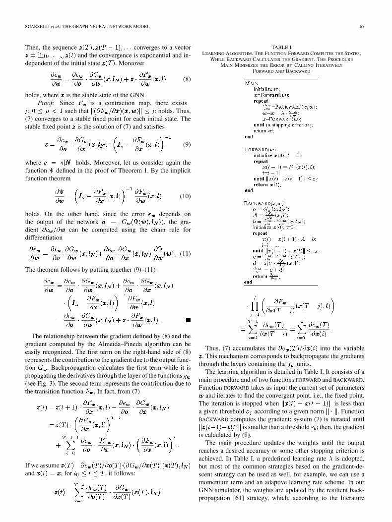
TABLE ILEARNING ALGORITHM. THE FUNCTION FORWARD COMPUTES THE STATES,

WHILE BACKWARD CALCULATES THE GRADIENT. THE PROCEDURE

MAIN MINIMIZES THE ERROR BY CALLING ITERATIVELY

FORWARD AND BACKWARD

Thus, (7) accumulates the into the variable. This mechanism corresponds to backpropagate the gradients

through the layers containing the units.The learning algorithm is detailed in Table I. It consists of a

main procedure and of two functions FORWARD and BACKWARD.Function FORWARD takes as input the current set of parameters

and iterates to find the convergent point, i.e., the fixed point.The iteration is stopped when is less thana given threshold according to a given norm . FunctionBACKWARD computes the gradient: system (7) is iterated until

is smaller than a threshold ; then, the gradientis calculated by (8).

The main procedure updates the weights until the outputreaches a desired accuracy or some other stopping criterion isachieved. In Table I, a predefined learning rate is adopted,but most of the common strategies based on the gradient-de-scent strategy can be used as well, for example, we can use amomentum term and an adaptive learning rate scheme. In ourGNN simulator, the weights are updated by the resilient back-propagation [61] strategy, which, according to the literature


on feedforward neural networks, is one of the most efficientstrategies for this purpose. On the other hand, the design oflearning algorithms for GNNs that are not explicitly based ongradient is not obvious and it is a matter of future research.In fact, the encoding network is only apparently similar to astatic feedforward network, because the number of the layersis dynamically determined and the weights are partially sharedaccording to input graph topology. Thus, second-order learningalgorithms [62], pruning [63], and growing learning algorithms[64]–[66] designed for static networks cannot be directlyapplied to GNNs. Other implementation details along witha computational cost analysis of the proposed algorithm areincluded in Section III.

D. Transition and Output Function Implementations

The implementation of the local output function does notneed to fulfill any particular constraint. In GNNs, is a mul-tilayered feedforward neural network. On the other hand, thelocal transition function plays a crucial role in the proposedmodel, since its implementation determines the number and theexistence of the solutions of (1). The assumption behind GNNis that the design of is such that the global transition func-tion is a contraction map w.r.t. the state . In the following,we describe two neural network models that fulfill this purposeusing different strategies. These models are based on the non-positional form described by (3). It can be easily observed thatthere exist two corresponding models based on the positionalform as well.

1) Linear (nonpositional) GNN. Equation (3) can naturally beimplemented by

(12)

where the vector and the matrixare defined by the output of two feedforward neural net-works (FNNs), whose parameters correspond to the param-eters of the GNN. More precisely, let us call transition net-work an FNN that has to generate and forcing net-work another FNN that has to generate . Moreover, let

and be the func-tions implemented by the transition and the forcing net-work, respectively. Then, we define

(13)

(14)

where and hold,and denotes the operator that allocates the ele-ments of a -dimensional vector into as matrix. Thus,

is obtained by arranging the outputs of the transitionnetwork into the square matrix and by multiplicationwith the factor . On the other hand, is justa vector that contains the outputs of the forcing network.Here, it is further assumed thatholds7; this can be straightforwardly verified if the outputneurons of the transition network use an appropriately

7The 1-norm of a matrix � � �� is defined as �� .

bounded activation function, e.g., a hyperbolic tangent.Note that in this case where is thevector constructed by stacking all the , and is a blockmatrix , with if is a neighbor of

and otherwise. Moreover, vectors andmatrices do not depend on the state , but only onnode and edge labels. Thus, , and, by simplealgebra

which implies that is a contraction map (w.r.t. )for any set of parameters .

2) Nonlinear (nonpositional) GNN. In this case, is real-ized by a multilayered FNN. Since three-layered neuralnetworks are universal approximators [67], can approx-imate any desired function. However, not all the parameters

can be used, because it must be ensured that the corre-sponding transition function is a contraction map. Thiscan be achieved by adding a penalty term to (6), i.e.,

where the penalty term is if and 0otherwise, and the parameter defines the desiredcontraction constant of . More generally, the penaltyterm can be any expression, differentiable w.r.t. , thatis monotone increasing w.r.t. the norm of the Jacobian.For example, in our experiments, we use the penalty term

, where is the th column of. In fact, such an expression is an approximation

of .

E. A Comparison With Random Walks andRecursive Neural Networks

GNNs turn out to be an extension of other models already pro-posed in the literature. In particular, recursive neural networks[17] are a special case of GNNs, where:

1) the input graph is a directed acyclic graph;2) the inputs of are limited to and , where

is the set of children of 8;3) there is a supersource node from which all the other

nodes can be reached. This node is typically used for output(graph-focused tasks).

The neural architectures, which have been suggested for real-izing and , include multilayered FNNs [17], [19], cascadecorrelation [68], and self-organizing maps [20], [69]. Note thatthe above constraints on the processed graphs and on the inputsof exclude any sort of cyclic dependence of a state on itself.Thus, in the recursive neural network model, the encoding net-works are FNNs. This assumption simplifies the computation of

8A node � is child of � if there exists an arc from � to �. Obviously, �� holds.


TABLE IITIME COMPLEXITY OF THE MOST EXPENSIVE INSTRUCTIONS OF THE LEARNING ALGORITHM. FOR EACH INSTRUCTION AND EACH GNN MODEL,

A BOUND ON THE ORDER OF FLOATING POINT OPERATIONS IS GIVEN. THE TABLE ALSO DISPLAYS

THE NUMBER OF TIMES PER EPOCH THAT EACH INSTRUCTION IS EXECUTED

the states. In fact, the states can be computed following a prede-fined ordering that is induced by the partial ordering of the inputgraph.

Interestingly, the GNN model captures also the random walkson graphs when choosing as a linear function. Random walksand, more generally, Markov chain models are useful in severalapplication areas and have been recently used to develop rankingalgorithms for internet search engines [18], [21]. In randomwalks on graphs, the state associated with a node is a realvalue and is described by

(15)

where is the set of parents of , and ,holds for each . The are normalized so that

. In fact, (15) can represent a random walkerwho is traveling on the graph. The value represents theprobability that the walker, when visiting node , decides to goto node . The state stands for the probability that the walkeris on node in the steady state. When all are stacked intoa vector , (15) becomes where andis defined as in (15) if and otherwise. It iseasily verified that . Markov chain theory suggeststhat if there exists such that all the elements of the matrixare nonnull, then (15) is a contraction map [70]. Thus, providedthat the above condition on holds, random walks on graphsare an instance of GNNs, where is a constant stochasticmatrix instead of being generated by neural networks.

III. COMPUTATIONAL COMPLEXITY ISSUES

In this section, an accurate analysis of the computational costwill be derived. The analysis will focus on three different GNNmodels: positional GNNs, where the functions and of (1)are implemented by FNNs; linear (nonpositional) GNNs; andnonlinear (nonpositional) GNNs.

First, we will describe with more details the most complexinstructions involved in the learning procedure (see Table II).Then, the complexity of the learning algorithm will be defined.For the sake of simplicity, the cost is derived assuming that thetraining set contains just one graph . Such an assumption doesnot cause any loss of generality, since the graphs of the trainingset can always be merged into a single graph. The complexity ismeasured by the order of floating point operations.9

In Table II, the notation is used to denote the number ofhidden-layer neurons. For example, indicates the number ofhidden-layer neurons in the implementation of function .

In the following, , , and denote the number of epochs,the mean number of forward iterations (of the repeat cycle infunction FORWARD), and the mean number of backward itera-tions (of the repeat cycle in function BACKWARD), respectively.Moreover, we will assume that there exist two proceduresand , which implement the forward phase and the backwardphase of the backpropagation procedure [71], respectively. For-mally, given a function implemented by anFNN, we have

Here, is the input vector and the row vector is asignal that suggests how the network output must be adjusted toimprove the cost function. In most applications, the cost func-tion is and ),where and is the vector of the desired output cor-responding to input . On the other hand, is thegradient of w.r.t. the network input and is easily computed

9According to the common definition of time complexity, an algorithm re-quires�� operations, if there exist� � �, �� , such that �� holds for each � � ��, where �� is the maximal number of operations executedby the algorithm when the length of input is �.


as a side product of backpropagation.10 Finally, and de-note the computational complexity required by the applicationof and on , respectively. For example, if is imple-mented by a multilayered FNN with inputs, hidden neurons,

and outputs, then holds.

A. Complexity of Instructions

1) Instructions , , and: Since is a matrix having at most

nonnull elements, the multiplication of by , and asa consequence, the instruction , costs

floating points operations. Moreover, the stateand the output vector are calculated by applying the local

transition function and the local output function to each node. Thus, in positional GNNs and in nonlinear GNNs, where ,

, and are directly implemented by FNNs, andare computed by running the forward phase of backpropagationonce for each node or edge (see Table II).

On the other hand, in linear GNNs, is calculated intwo steps: the matrices of (13) and the vectors (14) areevaluated; then, is computed. The former phase, the cost

of which is , is executed once for eachepoch, whereas the latter phase, the cost of which is ,is executed at every step of the cycle in the function FORWARD.

2) Instruction : This instruction re-quires the computation of the Jacobian of . Note that

is a block matrix where the block measures theeffect of node on node , if there is an arc from to

, and is null otherwise. In the linear model, the matricescorrespond to those displayed in (13) and used to calculatein the forward phase. Thus, such an instruction has no cost inthe backward phase in linear GNNs.

In nonlinear GNNs, ,is computed by appropriately exploiting the backpropagationprocedure. More precisely, let be a vector where allthe components are zero except for the th one, which equalsone, i.e., , , and so on.Note that , when it is applied to with , returns

, i.e., the th column of the Jacobian. Thus, can be computed by applying on

all the , i.e.,

(16)

where indicates that we are considering only the first com-ponent of the output of . A similar reasoning can also be usedwith positional GNNs. The complexity of these procedures iseasily derived and is displayed in the fourth row of Table II.

3) Computation of and : In linear GNNs,the cost function is , and, as a con-sequence, , if is a node belongingto the training set, and 0 otherwise. Thus, is easily cal-culated by operations.

10Backpropagation computes for each neuron � the delta value�� , where � is the cost function and � theactivation level of neuron �. Thus, �� is just a vector stacking allthe delta values of the input neurons.

In positional and nonlinear GNNs, a penalty term is addedto the cost function to force the transition function to be a con-traction map. In this case, it is necessary to compute ,because such a vector must be added to the gradient. Letdenote the element in position of the block . Accordingto the definition of , we have

where , if the sum is largerthan 0, and it is 0 otherwise. It follows:

where is the sign function. Moreover, let be a matrixwhose element in position is and let bethe operator that takes a matrix and produce a column vector bystacking all its columns one on top of the other. Then

(17)

holds. The vector depends on selected imple-mentation of or . For sake of simplicity, let us restrict ourattention to nonlinear GNNs and assume that the transition net-work is a three-layered FNN. , , , and are the activa-tion function11, the vector of the activation levels, the matrix ofthe weights, and the thresholds of the th layer, respectively. Thefollowing reasoning can also be extended to positional GNNsand networks with a different number of layers. The function

is formally defined in terms of , , , and

By the chain differentiation rule, it follows:

where is the derivative of , is an operator thattransforms a vector into a diagonal matrix having such a vectoras diagonal, and is the submatrix of that contains onlythe weights that connect the inputs corresponding to tothe hidden layer. The parameters affect four components of

11 is a vectorial function that takes as input the vector of the activationlevels of neurons in a layer and returns the vector of the outputs of the neuronsof the same layer.


, i.e., , , , and . By properties of derivativesfor matrix products and the chain rule

(18)

holds.Thus, is the sum of four con-

tributions. In order to derive a method to compute those terms,let denote the identity matrix. Let be the Kro-necker product and suppose that is a matrix suchthat for any vector . By the Kro-necker product properties, holdsfor matrices , , and having compatible dimensions [72].Thus, we have

which implies

Similarly, using the propertiesand , it follows:

where is the number of hidden neurons. Then, we have

(19)

(20)

(21)

(22)

where the mentioned Kronecker product properties have beenused.

It follows that can be writtenas the sum of the four contributions represented by (19)–(22).The second and the fourth term [(20) and (22)] can be computeddirectly using the corresponding formulas. The first one can becalculated by observing that looks like the function com-puted by a three-layered FNN that is the same as except forthe activation function of the last layer. In fact, if we denote by

such a network, then

(23)

holds, where . A sim-ilar reasoning can be applied also to the third contribution.

The above described method includes two tasks: the matrixmultiplications of (19)–(22) and the backpropagation as definedby (23). The former task consists of several matrix multiplica-tions. By inspection of (19)–(22), the number of floating pointoperations is approximately estimated as

,12 where denotes the number of hidden-layer neu-rons implementing the function . The second task has approx-imately the same cost as a backpropagation phase through theoriginal function .

Thus, the complexity of computing is

. Note, however, that even if the sum in (17)ranges over all the arcs of the graph, only those arcs suchthat have to be considered. In practice,is a rare event, since it happens only when the columns of theJacobian are larger than and a penalty function was usedto limit the occurrence of these cases. As a consequence, abetter estimate of the complexity of computing is

, where is the average number ofnodes such that holds for some .

4) Instructions and: The terms and can be

calculated by the backpropagation of through thenetwork that implements . Since such an operation mustbe repeated for each node, the time complexity of instruc-tions and

is for all the GNN models.

12Such a value is obtained by considering the following observations: for an� � � matrix �� and � � � matrix ��, the multiplication �� requires approxi-mately �� operations; more precisely,��multiplications and�� sums.If�� is a diagonal �� matrix, then�� requires �� operations. Moreover, if�� is an �� matrix, �� is a �� matrix, and �� is the � � � matrix definedabove and used in (19)–(22), then computing �� costs only �� op-erations provided that a sparse representation is used for � . Finally, ��

are already available, since they are computed during the forward phase of thelearning algorithm.


5) Instruction : By definition of, , and , we have

(24)

where and indicates that we areconsidering only the first part of the output of . Similarly

(25)

where . Thus, (24) and (25) provide adirect method to compute in positional and nonlinear GNNs,respectively.

For linear GNNs, let denote the th output of and notethat

holds. Here, and are the element in position of ma-trix and the corresponding output of the transition network[see (13)], respectively, while is the th element of vector ,

is the corresponding output of the forcing network [see (14)],and is the th element of . Then

where , , , and isa vector that stores in the position corre-sponding to , that is, . Thus,in linear GNNs, is computed by calling the backpropagationprocedure on each arc and node.

B. Time Complexity of the GNN Model

According to our experiments, the application of a trainedGNN on a graph (test phase) is relatively fast even for largegraphs. Formally, the complexity is easily derived from

Table II and it is for positional

GNNs, for nonlinear GNNs, and

for linear GNNs.In practice, the cost of the test phase is mainly due to therepeated computation of the state . The cost of each it-eration is linear both w.r.t. the dimension of the input graph(the number of edges), the dimension of the employed FNNsand the state, with the only exception of linear GNNs, whosesingle iteration cost is quadratic w.r.t. to the state. The numberof iterations required for the convergence of the state dependson the problem at hand, but Banach’s theorem ensures that theconvergence is exponentially fast and experiments have shownthat 5–15 iterations are generally sufficient to approximate thefixed point.

In positional and nonlinear GNNs, the transition functionmust be activated and times, respectively. Evenif such a difference may appear significant, in practice, thecomplexity of the two models is similar, because the networkthat implements the is larger than the one that implements

. In fact, has input neurons, where isthe maximum number of neighbors for a node, whereashas only input neurons. An appreciable difference canbe noticed only for graphs where the number of neighborsof nodes is highly variable, since the inputs of must besufficient to accommodate the maximal number of neighborsand many inputs may remain unused when is applied. Onthe other hand, it is observed that in the linear model the FNNsare used only once for each iteration, so that the complexity

of each iteration is instead of . Note that

holds, when isimplemented by a three-layered FNN with hidden neurons.In practical cases, where is often larger than , the linearmodel is faster than the nonlinear model. As confirmed by theexperiments, such an advantage is mitigated by the smalleraccuracy that the model usually achieves.

In GNNs, the learning phase requires much more time thanthe test phase, mainly due to the repetition of the forward andbackward phases for several epochs. The experiments haveshown that the time spent in the forward and backward phasesis not very different. Similarly to the forward phase, the costof function BACKWARD is mainly due to the repetition of theinstruction that computes . Theorem 2 ensures thatconverges exponentially fast and the experiments confirmedthat is usually a small number.

Formally, the cost of each learning epoch is given by the sumof all the instructions times the iterations in Table II. An inspec-tion of Table II shows that the cost of all instructions involved inthe learning phase are linear both with respect to the dimensionof the input graph and of the FNNs. The only exceptions are dueto the computation of ,and , which depend quadratically on .

The most expensive instruction is apparently the computa-tion of in nonlinear GNNs, which costs

. On the other hand, the experiments have shown thatusually is a small number. In most epochs, is 0, sincethe Jacobian does not violate the imposed constraint, and inthe other cases, is usually in the range 1–5. Thus, for a


small state dimension , the computation of requiresfew applications of backpropagation on and has a small im-pact on the global complexity of the learning process. On theother hand, in theory, if is very large, it might happen that

and at the same time, causing the computation of the gradient to be very

slow. However, it is worth mentioning that this case was neverobserved in our experiments.

IV. EXPERIMENTAL RESULTS

In this section, we present the experimental results, obtainedon a set of simple problems carried out to study the propertiesof the GNN model and to prove that the method can be ap-plied to relevant applications in relational domains. The prob-lems that we consider, viz., the subgraph matching, the mutage-nesis, and the web page ranking, have been selected since theyare particularly suited to discover the properties of the modeland are correlated to important real-world applications. Froma practical point of view, we will see that the results obtainedon some parts of mutagenesis data sets are among the best thatare currently reported in the open literature (please see detailedcomparison in Section IV-B). Moreover, the subgraph matchingproblem is relevant to several application domains. Even if theperformance of our method is not comparable in terms of bestaccuracy on the same problem with the most efficient algorithmsin the literature, the proposed approach is a very general tech-nique that can be applied on extension of the subgraph matchingproblems [73]–[75]. Finally, the web page ranking is an inter-esting problem, since it is important in information retrieval andvery few techniques have been proposed for its solution [76]. Itis worth mentioning that the GNN model has been already suc-cessfully applied on larger applications, which include imageclassification and object localization in images [77], [78], webpage ranking [79], relational learning [80], and XML classifica-tion [81].

The following facts hold for each experiment, unless other-wise specified. The experiments have been carried out with bothlinear and nonlinear GNNs. According to existing results on re-cursive neural networks, the nonpositional transition functionslightly outperforms the positional ones, hence, currently onlynonpositional GNNs have been implemented and tested. Boththe (nonpositional) linear and the nonlinear model were tested.All the functions involved in the two models, i.e., , , and

for linear GNNs, and and for nonlinear GNNs wereimplemented by three-layered FNNs with sigmoidal activationfunctions. The presented results were averaged over five dif-ferent runs. In each run, the data set was a collection of randomgraphs constructed by the following procedure: each pair ofnodes was connected with a certain probability ; the resultinggraph was checked to verify whether it was connected and ifit was not, random edges were inserted until the condition wassatisfied.

The data set was split into a training set, a validation set, anda test set and the validation set was used to avoid possible issueswith overfitting. For the problems where the original data is onlyone single big graph , a training set, a validation set, and a test

Fig. 4. Two graphs�� and�� that contain a subgraph ��. The numbers insidethe nodes represent the labels. The function � to be learned is �� ,if � is a black node, and �� , if � is a white node.

set include different supervised nodes of . Otherwise, whenseveral graphs were available, all the patterns of a graph wereassigned to only one set. In every trial, the training procedureperformed at most 5000 epochs and every 20 epochs the GNNwas evaluated on the validation set. The GNN that achieved thelowest cost on the validation set was considered the best modeland was applied to the test set.

The performance of the model is measured by the accuracyin classification problems (when can take only the values

or 1) and by the relative error in regression problems (whenmay be any real number). More precisely, in a classifi-

cation problem, a pattern is considered correctly classified ifand or if and

. Thus, accuracy is defined as the percentage ofpatterns correctly classified by the GNN on the test set. Onthe other hand, in regression problems, the relative error on apattern is given by .

The algorithm was implemented in Matlab® 713 and the soft-ware can be freely downloaded, together with the source andsome examples [82]. The experiments were carried out on aPower Mac G5 with a 2-GHz PowerPC processor.

A. The Subgraph Matching Problem

The subgraph matching problem consists of finding the nodesof a given subgraph in a larger graph . More precisely, thefunction that has to be learned is such thatif belongs to a subgraph of , which is isomorphic to

, and , otherwise (see Fig. 4). Subgraphmatching has a number of practical applications, such as ob-ject localization and detection of active parts in chemical com-pounds [73]–[75]. This problem is a basic test to assess a methodfor graph processing. The experiments will demonstrate thatthe GNN model can cope with the given task. Of course, thepresented results cannot be compared with those achievable byother specific methods for subgraph matching, which are fasterand more accurate. On the other hand, the GNN model is a gen-eral approach and can be used without any modification to avariety of extensions of the subgraph matching problem, where,for example, several graphs must be detected at the same time,the graphs are corrupted by noise on the structure and the labels,

13Copyright © 1994–2006 by The MathWorks, Inc., Natick, MA.


TABLE IIIACCURACIES ACHIEVED BY NONLINEAR MODEL (NL), LINEAR MODEL

(L), AND A FEEDFORWARD NEURAL NETWORK

ON SUBGRAPH MATCHING PROBLEM

and the target to be detected is unknown and provided only byexamples.

In our experiments, the data set consisted of 600 connectedrandom graphs (constructed using ), equally divided intoa training set, a validation set, and a test set. A smaller subgraph

, which was randomly generated in each trial, was inserted intoevery graph of the data set. Thus, each graph contained atleast a copy of , even if more copies might have been includedby the random construction procedure. All the nodes had integerlabels in the range and, in order to define the correct tar-gets , a brute force algorithm located all thecopies of in . Finally, a small Gaussian noise, with zeromean and a standard deviation of 0.25, was added to all the la-bels. As a consequence, all the copies of in our data set weredifferent due to the introduced noise.

In all the experiments, the state dimension was and allthe neural networks involved in the GNNs had five hidden neu-rons. More network architectures have been tested with similarresults.

In order to evaluate the relative importance of the labels andthe connectivity in the subgraph localization, also a feedforwardneural network was applied to this test. The FNN had one output,20 hidden, and one input units. The FNN predicted usingonly the label of node . Thus, the FNN did not use theconnectivity and exploited only the relative distribution of thelabels in w.r.t. the labels in graphs .

Table III presents the accuracies achieved by the nonlinearGNN model (nonlinear), the linear GNN model (linear), and theFNN with several dimensions for and . The results allow tosingle out some of the factors that have influence on the com-plexity of the problem and on the performance of the models.Obviously, the proportion of positive and negative patterns af-fects the performance of all the methods. The results improvewhen is close to , whereas when is about a half of

, the performance is lower. In fact, in the latter case, the dataset is perfectly balanced and it is more difficult to guess the right

response. Moreover, the dimension , by itself, has influenceon the performance, because the labels can assume only 11 dif-ferent values and when is small most of the nodes of the sub-graph can be identified by their labels. In fact, the performancesare better for smaller , even if we restrict our attention to thecases when holds.

The results show that GNNs always outperform the FNNs,confirming that the GNNs can exploit label contents and graphtopology at the same time. Moreover, the nonlinear GNN modelachieved a slightly better performance than the linear one, prob-ably because nonlinear GNNs implement a more general modelthat can approximate a larger class of functions. Finally, it canbe observed that the total average error for FNNs is about 50%larger than the GNN error (12.7 for nonlinear GNNs, 13.5 forlinear GNNs, and 22.8 for FNNs). Actually, the relative differ-ence between the GNN and FNN errors, which measures theadvantage provided by the topology, tend to become smallerfor larger values of (see the last column of Table III). Infact, GNNs use an information diffusion mechanism to decidewhether a node belongs to the subgraph. When is larger, moreinformation has to be diffused and, as a consequence, the func-tion to be learned is more complex.

The subgraph matching problem was used also to evaluate theperformance of the GNN model and to experimentally verify thefindings about the computational cost of the model describedin Section III. For this purpose, some experiments have beencarried out varying the number of nodes, the number of edgesin the data set, the number of hidden units in the neural networksimplementing the GNN, and the dimensionality of the state. Inthe base case, the training set contained ten random graphs, eachone made of 20 nodes and 40 edges, the networks implementingthe GNN had five hidden neurons, and the state dimension was2. The GNN was trained for 1000 epochs and the results wereaveraged over ten trials. As expected, the central processing unit(CPU) time required by the gradient computation grows linearlyw.r.t. the number of nodes, edges and hidden units, whereasthe growth is quadratic w.r.t. the state dimension. For example,Fig. 5 depicts the CPU time spent by the gradient computationprocess when the nodes of each graph14 [Fig. 5(a)] and the statesof the GNN [Fig. 5(b)] are increased, respectively.

It is worth mentioning that, in nonlinear GNNs, thequadratic growth w.r.t. the states, according to the discus-sion of Section III, depends on the time spent to calculate theJacobian and its derivative . Fig. 5shows how the total time spent by the gradient computationprocess is composed in this case: line denotes the timerequired by the computation of and ; line de-notes that for the Jacobian ; line denotesthat for the derivative ; the dotted line and the dashedline represent the rest of the time15 required by the FORWARD

and the BACKWARD procedure, respectively; the continuousline stands for the rest of the time required by the gradientcomputation process.

14More precisely, in this experiment, nodes and edges were increased keepingconstant to �� their ratio.

15That is, the time required by those procedures except for that already con-sidered in the previous points.


Fig. 5. Some plots about the cost of the gradient computation on GNNs. (a) and (b) CPU times required for 1000 learning epochs by nonlinear GNNs (continuousline) and linear GNN (dashed line), respectively, as a function of the number of nodes of the training set (a) and the dimension of the state (b). (c) Compositionof the learning time for nonlinear GNNs: the computation of � and �� (��); the Jacobian �� (� � �); the derivative � �� (��);the rest of the FORWARD procedure (dotted line); the rest of the BACKWARD procedure (dashed line); the rest of the time learning procedure (continuous line).(d) Histogram of the number of the forward iterations, the backward iterations, and the number of nodes � such that �� [see (17)] encountered in eachepoch of a learning session.

From Fig. 5(c), we can observe that the computation ofthat, in theory, is quadratic w.r.t. the states may have a

small effect in practice. In fact, as already noticed in Section III,the cost of such a computation depends on the number ofcolumns of whose norm is larger than theprescribed threshold, i.e., the number of nodes and suchthat [see (17)]. Such a number is usually small due tothe effect of the penalty term . Fig. 5(d) shows a histogramof the number of nodes for which in each epochof a learning session: in practice, in this experiment, the non-null are often zero and never exceed four in magnitude.Another factor that affects the learning time is the number offorward and backward iterations needed to compute the stablestate and the gradient, respectively.16 Fig. 5(d) shows also the

16The number of iterations depends also on the constant and of Table I,which were both set to �� in the experiments. However, due to the exponen-tial convergence of the iterative methods, these constants have a linear effect.

histograms of the number of required iterations, suggesting thatalso those numbers are often small.

B. The Mutagenesis Problem

The Mutagenesis data set [13] is a small data set, which isavailable online and is often used as a benchmark in the re-lational learning and inductive logic programming literature.It contains the descriptions of 230 nitroaromatic compoundsthat are common intermediate subproducts of many industrialchemical reactions [83]. The goal of the benchmark consists oflearning to recognize the mutagenic compounds. The log mu-tagenicity was thresholded at zero, so the prediction is a bi-nary classification problem. We will demonstrate that GNNsachieved the best result compared with those reported in the lit-erature on some parts of the data set.


Fig. 6. Atom-bond structure of a molecule represented by a graph with labelednodes. Nodes represent atoms and edges denote atom bonds. Only one node issupervised.

In [83], it is shown that 188 molecules out of 230 areamenable to a linear regression analysis. This subset was called“regression friendly,” while the remaining 42 compounds weretermed “regression unfriendly.” Many different features havebeen used in the prediction. Apart from the atom-bond (AB)structure, each compound is provided with four global features[83]. The first two features are chemical measurements (C):the lowest unoccupied molecule orbital and the water/octanolpartition coefficient, while the remaining two are precodedstructural (PS) attributes. Finally, the AB description can beused to define functional groups (FG), e.g., methyl groups andmany different rings that can be used as higher level features.In our experiments, the best results were achieved using AB,C, and PS, without the functional groups. Probably the reasonis that GNNs can recover the substructures that are relevant tothe classification, exploiting the graphical structure containedin the AB description.

In our experiments, each molecule of the data set was trans-formed into a graph where nodes represent atoms and edgesstand for ABs. The average number of nodes in a molecule isaround 26. Node labels contain atom type, its energy state, andthe global properties AB, C, and PS. In each graph, there isonly one supervised node, the first atom in the AB description(Fig. 6). The desired output is 1, if the molecule is mutagenic,and 1, otherwise.

In Tables IV–VI, the results obtained by nonlinear GNNs17

are compared with those achieved by other methods. The pre-sented results were evaluated using a tenfold cross-validationprocedure, i.e., the data set was randomly split into ten parts andthe experiments were repeated ten times, each time using a dif-ferent part as the test set and the remaining patterns as trainingset. The results were averaged on five runs of the cross-valida-tion procedure.

GNNs achieved the best accuracy on the regression-un-friendly part (Table V) and on the whole data set (Table VI),while the results are close to the state of the art techniqueson the regression-friendly part (Table IV). It is worth noticingthat, whereas most of the approaches showed a higher level ofaccuracy when applied to the whole data set with respect to the

17Some results were already presented in [80].

TABLE IVACCURACIES ACHIEVED ON THE REGRESSION-FRIENDLY PART OF THE

MUTAGENESIS DATA SET. THE TABLE DISPLAYS THE METHOD, THE

FEATURES USED TO MAKE THE PREDICTION, AND A POSSIBLE

REFERENCE TO THE PAPER WHERE THE RESULT IS DESCRIBED

TABLE VACCURACIES ACHIEVED ON THE REGRESSION-UNFRIENDLY PART OF THE

MUTAGENESIS DATA SET. THE TABLE DISPLAYS THE METHOD, THE

FEATURES USED TO MAKE THE PREDICTION, AND A POSSIBLE

REFERENCE TO THE PAPER WHERE THE RESULT IS DESCRIBED

TABLE VIACCURACIES ACHIEVED ON THE WHOLE MUTAGENESIS DATA SET. THE TABLE

DISPLAYS THE METHOD, THE FEATURES USED TO MAKE THE PREDICTION, AND

A POSSIBLE REFERENCE TO THE PAPER WHERE THE RESULT IS DESCRIBED

unfriendly part, the converse holds for GNNs. This suggests thatGNNs can capture characteristics of the patterns that are usefulto solve the problem but are not homogeneously distributed inthe two parts.

C. Web Page Ranking

In this experiment, the goal is to learn the rank of a webpage, inspired by Google’s PageRank [18]. According toPageRank, a page is considered authoritative if it is referredby many other pages and if the referring pages are authori-tative themselves. Formally, the PageRank of a page is

where is the outdegreeof , and is the damping factor [18]. In this experi-ment, it is shown that a GNN can learn a modified version ofPageRank, which adapts the “authority” measure accordingto the page content. For this purpose, a random web graph


Fig. 7. Desired function � (the continuous lines) and the output of the GNN (the dotted lines) on the pages that belong to only one topic (a) and on the other pages(b). Horizontal axis stands for pages and vertical axis stands for scores. Pages have been sorted according to the desired value ��.

containing 5000 nodes was generated, with . Training,validation, and test sets consisted of different nodes of thisgraph. More precisely, only 50 nodes were supervised in thetraining set, other 50 nodes belonged to the validation set, andthe remaining nodes were in the test set.

To each node , a bidimensional boolean label is at-tached that represents whether the page belongs to two giventopics. If the page belongs to both topics, then

, while if it belongs to only one topic, then ,or , and if it does not belong to either topics, then

. The GNN was trained in order to produce thefollowing output:

ifotherwise

where stands for the Google’s PageRank.Web page ranking algorithms are used by search engines to

sort the URLs returned in response to user’s queries and moregenerally to evaluate the data returned by information retrievalsystems. The design of ranking algorithms capable of mixing to-gether the information provided by web connectivity and pagecontent has been a matter of recent research [93]–[96]. In gen-eral, this is an interesting and hard problem due to the difficultyin coping with structured information and large data sets. Here,we present the results obtained by GNNs on a synthetic data set.More results achieved on a snapshot of the web are available in[79].

For this example, only the linear model has been used, be-cause it is naturally suited to approximate the linear dynamicsof the PageRank. Moreover, the transition and forcing networks(see Section I) were implemented by three-layered neural net-works with five hidden neurons, and the dimension of the statewas . For the output function, is implemented as

where is the function realizedby a three-layered neural networks with five hidden neurons.

Fig. 7 shows the output of the GNN and the target functionon the test set. Fig. 7(a) displays the result for the pages that

belong to only one topic and Fig. 7(b) displays the result forthe other pages. Pages are displayed on horizontal axes and aresorted according to the desired output . The plots denote

Fig. 8. Error function on the training set (continuous line) and on the validation(dashed line) set during learning phase.

the value of function (continuous lines) and the value of thefunction implemented by the GNN (the dotted lines). The figureclearly suggests that GNN performs very well on this problem.

Finally, Fig. 8 displays the error function during the learningprocess. The continuous line is the error on the training set,whereas the dotted line is the error on the validation set. Itis worth noting that the two curves are always very close andthat the error on the validation set is still decreasing after 2400epochs. This suggests that the GNN does not experiment over-fitting problems, despite the fact that the learning set consists ofonly 50 pages from a graph containing 5000 nodes.

V. CONCLUSION

In this paper, we introduced a novel neural network modelthat can handle graph inputs: the graphs can be cyclic, directed,undirected, or a mixture of these. The model is based on in-formation diffusion and relaxation mechanisms. The approachextends into a common framework, the previous connectionisttechniques for processing structured data, and the methodsbased on random walk models. A learning algorithm to esti-mate model parameters was provided and its computationalcomplexity was studied, demonstrating that the method issuitable also for large data sets.


Some promising experimental results were provided to assessthe model. In particular, the results achieved on the whole Mu-tagenisis data set and on the unfriendly part of such a data setare the best compared with those reported in the open literature.Moreover, the experiments on the subgraph matching and on theweb page ranking show that the method can be applied to prob-lems that are related to important practical applications.

The possibility of dealing with domains where the data con-sists of patterns and relationships gives rise to several new topicsof research. For example, while in this paper it is assumed thatthe domain is static, it may happen that the input graphs changewith time. In this case, at least two interesting issues can beconsidered: first, GNNs must be extended to cope with a dy-namic domain; and second, no method exists, to the best of ourknowledge, to model the evolution of the domain. The solutionof the latter problem, for instance, may allow to model the evolu-tion of the web and, more generally, of social networks. Anothertopic of future research is the study on how to deal with domainswhere the relationships, which are not known in advance, mustbe inferred. In this case, the input contains flat data and is auto-matically transformed into a set of graphs in order to shed somelight on possible hidden relationships.

REFERENCES

[1] P. Baldi and G. Pollastri, “The principled design of large-scale recur-sive neural network architectures-dag-RNNs and the protein structureprediction problem,” J. Mach. Learn. Res., vol. 4, pp. 575–602, 2003.

[2] E. Francesconi, P. Frasconi, M. Gori, S. Marinai, J. Sheng, G. Soda, andA. Sperduti, “Logo recognition by recursive neural networks,” in Lec-ture Notes in Computer Science — Graphics Recognition, K. Tombreand A. K. Chhabra, Eds. Berlin, Germany: Springer-Verlag, 1997.

[3] E. Krahmer, S. Erk, and A. Verleg, “Graph-based generation of refer-ring expressions,” Comput. Linguist., vol. 29, no. 1, pp. 53–72, 2003.

[4] A. Mason and E. Blake, “A graphical representation of the state spacesof hierarchical level-of-detail scene descriptions,” IEEE Trans. Vis.Comput. Graphics, vol. 7, no. 1, pp. 70–75, Jan.-Mar. 2001.

[5] L. Baresi and R. Heckel, “Tutorial introduction to graph transforma-tion: A software engineering perspective,” in Lecture Notes in Com-puter Science. Berlin, Germany: Springer-Verlag, 2002, vol. 2505,pp. 402–429.

[6] C. Collberg, S. Kobourov, J. Nagra, J. Pitts, and K. Wampler, “A systemfor graph-based visualization of the evolution of software,” in Proc.ACM Symp. Software Vis., 2003, pp. 77–86.

[7] A. Bua, M. Gori, and F. Santini, “Recursive neural networks appliedto discourse representation theory,” in Lecture Notes in Computer Sci-ence. Berlin, Germany: Springer-Verlag, 2002, vol. 2415.

[8] L. De Raedt, Logical and Relational Learning. New York: Springer-Verlag, 2008, to be published.

[9] T. Dietterich, L. Getoor, and K. Murphy, Eds., Proc. Int. WorkshopStatist. Relat. Learn. Connect. Other Fields, 2004.

[10] P. Avesani and M. Gori, Eds., Proc. Int. Workshop Sub-Symbol.Paradigms Structured Domains, 2005.

[11] S. Nijseen, Ed., Proc. 3rd Int. Workshop Mining Graphs Trees Se-quences, 2005.

[12] T. Gaertner, G. Garriga, and T. Meini, Eds., Proc. 4th Int. WorkshopMining Graphs Trees Sequences, 2006.

[13] A. Srinivasan, S. Muggleton, R. King, and M. Sternberg, “Mutagenesis:Ilp experiments in a non-determinate biological domain,” in Proc. 4thInt. Workshop Inductive Logic Programm., 1994, pp. 217–232.

[14] T. Pavlidis, Structural Pattern Recognition, ser. Electrophysics. NewYork: Springer-Verlag, 1977.

[15] M. Bianchini, M. Maggini, L. Sarti, and F. Scarselli, “Recursive neuralnetworks learn to localize faces,” Phys. Rev. Lett., vol. 26, no. 12, pp.1885–1895, Sep. 2005.

[16] S. Haykin, Neural Networks: A Comprehensive Foundation. NewYork: Prentice-Hall, 1994.

[17] P. Frasconi, M. Gori, and A. Sperduti, “A general framework for adap-tive processing of data structures,” IEEE Trans. Neural Netw., vol. 9,no. 5, pp. 768–786, Sep. 1998.

[18] S. Brin and L. Page, “The anatomy of a large-scale hypertextual websearch engine,” in Proc. 7th World Wide Web Conf., Apr. 1998, pp.107–117.

[19] A. Sperduti and A. Starita, “Supervised neural networks for the clas-sification of structures,” IEEE Trans. Neural Netw., vol. 8, no. 2, pp.429–459, Mar. 1997.

[20] M. Hagenbuchner, A. Sperduti, and A. C. Tsoi, “A self-organizing mapfor adaptive processing of structured data,” IEEE Trans. Neural Netw.,vol. 14, no. 3, pp. 491–505, May 2003.

[21] J. Kleinberg, “Authoritative sources in a hyperlinked environment,” J.ACM, vol. 46, no. 5, pp. 604–632, 1999.

[22] A. C. Tsoi, G. Morini, F. Scarselli, M. Hagenbuchner, and M. Maggini,“Adaptive ranking of web pages,” in Proc. 12th World Wide Web Conf.,Budapest, Hungary, May 2003, pp. 356–365.

[23] M. Bianchini, P. Mazzoni, L. Sarti, and F. Scarselli, “Face spotting incolor images using recursive neural networks,” in Proc. 1st Int. Work-shop Artif. Neural Netw. Pattern Recognit., Florence, Italy, Sep. 2003,pp. 76–81.

[24] M. Bianchini, M. Gori, and F. Scarselli, “Processing directed acyclicgraphs with recursive neural networks,” IEEE Trans. Neural Netw., vol.12, no. 6, pp. 1464–1470, Nov. 2001.

[25] A. Küchler and C. Goller, “Inductive learning in symbolic domainsusing structure-driven recurrent neural networks,” in Lecture Notes inComputer Science, G. Görz and S. Hölldobler, Eds. Berlin, Germany:Springer-Verlag, Sep. 1996, vol. 1137.

[26] T. Schmitt and C. Goller, “Relating chemical structure to activity:An application of the neural folding architecture,” in Proc. WorkshopFuzzy-Neuro Syst./Conf. Eng. Appl. Neural Netw., 1998, pp. 170–177.

[27] M. Hagenbuchner and A. C. Tsoi, “A supervised training algorithmfor self-organizing maps for structures,” Pattern Recognit. Lett., vol.26, no. 12, pp. 1874–1884, 2005.

[28] M. Gori, M. Maggini, E. Martinelli, and F. Scarselli, “Learning userprofiles in NAUTILUS,” in Proc. Int. Conf. Adaptive HypermediaAdaptive Web-Based Syst., Trento, Italy, Aug. 2000, pp. 323–326.

[29] M. Bianchini, P. Mazzoni, L. Sarti, and F. Scarselli, “Face spotting incolor images using recursive neural networks,” in Proc. Italian Work-shop Neural Netw., Vietri sul Mare, Italy, Jul. 2003.

[30] B. Hammer and J. Jain, “Neural methods for non-standard data,” inProc. 12th Eur. Symp. Artif. Neural Netw., M. Verleysen, Ed., 2004,pp. 281–292.

[31] T. Gärtner, “Kernel-based learning in multi-relational data mining,”ACM SIGKDD Explorations, vol. 5, no. 1, pp. 49–58, 2003.

[32] T. Gärtner, J. Lloyd, and P. Flach, “Kernels and distances for structureddata,” Mach. Learn., vol. 57, no. 3, pp. 205–232, 2004.

[33] R. Kondor and J. Lafferty, “Diffusion kernels on graphs and other dis-crete structures,” in Proc. 19th Int. Conf. Mach. Learn., C. Sammut andA. e. Hoffmann, Eds., 2002, pp. 315–322.

[34] H. Kashima, K. Tsuda, and A. Inokuchi, “Marginalized kernelsbetween labeled graphs,” in Proc. 20th Int. Conf. Mach. Learn., T.Fawcett and N. e. Mishra, Eds., 2003, pp. 321–328.

[35] P. Mahé, N. Ueda, T. Akutsu, J.-L Perret, and J.-P. Vert, “Extensionsof marginalized graph kernels,” in Proc. 21st Int. Conf. Mach. Learn.,2004, pp. 552–559.

[36] M. Collins and N. Duffy, “Convolution kernels for natural language,”in Advances in Neural Information Processing Systems, T. G. Diet-terich, S. Becker, and Z. Ghahramani, Eds. Cambridge, MA: MITPress, 2002, vol. 14, pp. 625–632.

[37] J. Suzuki, Y. Sasaki, and E. Maeda, “Kernels for structured naturallanguage data,” in Proc. Conf. Neural Inf. Process. Syst., 2003.

[38] J. Suzuki, H. Isozaki, and E. Maeda, “Convolution kernels with fea-ture selection for natural language processing tasks,” in Proc. Annu.Meeting Assoc. Comput. Linguistics, 2004, pp. 119–126.

[39] J. Cho, H. Garcia-Molina, and L. Page, “Efficient crawling through urlordering,” in Proc. 7th World Wide Web Conf., Brisbane, Australia, Apr.1998, pp. 161–172.

[40] A. C. Tsoi, M. Hagenbuchner, and F. Scarselli, “Computing cus-tomized page ranks,” ACM Trans. Internet Technol., vol. 6, no. 4, pp.381–414, Nov. 2006.

[41] H. Chang, D. Cohn, and A. K. McCallum, “Learning to create cus-tomized authority lists,” in Proc. 17th Int. Conf. Mach. Learn., 2000,pp. 127–134.

[42] J. Lafferty, A. McCallum, and F. Pereira, “Conditional random fields:Probabilistic models for segmenting and labeling sequence data,” inProc. 18th Int. Conf. Mach. Learn., 2001, pp. 282–289.


[43] F. V. Jensen, Introduction to Bayesian Networks. New York:Springer-Verlag, 1996.

[44] L. Getoor and B. Taskar, Introduction to Statistical RelationalLearning. Cambridge, MA: MIT Press, 2007.

[45] V. N. Vapnik, Statistical Learning Theory. New York: Wiley, 1998.[46] O. Chapelle, B. Schölkopf, and A. Zien, Eds., Semi-Supervised

Learning. Cambridge, MA: MIT Press, 2006.[47] L. Chua and L. Yang, “Cellular neural networks: Theory,” IEEE Trans.

Circuits Syst., vol. CAS-35, no. 10, pp. 1257–1272, Oct. 1988.[48] L. Chua and L. Yang, “Cellular neural networks: Applications,” IEEE

Trans. Circuits Syst., vol. CAS-35, no. 10, pp. 1273–1290, Oct. 1988.[49] P. Kaluzny, “Counting stable equilibria of cellular neural networks-A

graph theoretic approach,” in Proc. Int. Workshop Cellular NeuralNetw. Appl., 1992, pp. 112–116.

[50] M. Ogorzatek, C. Merkwirth, and J. Wichard, “Pattern recognitionusing finite-iteration cellular systems,” in Proc. 9th Int. WorkshopCellular Neural Netw. Appl., 2005, pp. 57–60.

[51] J. Hopfield, “Neural networks and physical systems with emergentcollective computational abilities,” Proc. Nat. Acad. Sci., vol. 79, pp.2554–2558, 1982.

[52] F. Scarselli, M. Gori, A. C. Tsoi, M. Hagenbuchner, and G. Monfar-dini, “Computation capabilities of graph neural networks,” IEEE Trans.Neural Netw., vol. 20, no. 1, Jan. 2009, to be published.

[53] M. A. Khamsi, An Introduction to Metric Spaces and Fixed PointTheory. New York: Wiley, 2001.

[54] M. Bianchini, M. Maggini, L. Sarti, and F. Scarselli, “Recursive neuralnetworks for processing graphs with labelled edges: Theory and appli-cations,” Neural Netw., vol. 18, Special Issue on Neural Networks andKernel Methods for Structured Domains, no. 8, pp. 1040–1050, 2005.

[55] M. J. D. Powell, “An efficient method for finding the minimum of afunction of several variables without calculating derivatives,” Comput.J., vol. 7, pp. 155–162, 1964.

[56] W. T. Miller, III, R. Sutton, and P. E. Werbos, Neural Network forControl. Camrbidge, MA: MIT Press, 1990.

[57] A. C. Tsoi, “Adaptive processing of sequences and data structures,” inLecture Notes in Computer Science, C. L. Giles and M. Gori, Eds.Berlin, Germany: Springer-Verlag, 1998, vol. 1387, pp. 27–62.

[58] L. Almeida, “A learning rule for asynchronous perceptrons with feed-back in a combinatorial environment,” in Proc. IEEE Int. Conf. NeuralNetw., M. Caudill and C. Butler, Eds., San Diego, 1987, vol. 2, pp.609–618.

[59] F. Pineda, “Generalization of back-propagation to recurrent neural net-works,” Phys. Rev. Lett., vol. 59, pp. 2229–2232, 1987.

[60] W. Rudin, Real and Complex Analysis, 3rd ed. New York: McGraw-Hill, 1987.

[61] M. Riedmiller and H. Braun, “A direct adaptive method for faster back-propagation learning: The rprop algorithm,” in Proc. IEEE Int. Conf.Neural Netw., San Francisco, CA, 1993, pp. 586–591.

[62] M. Bishop, Neural Networks for Pattern Recognition. Oxford, U.K.:Oxford Univ. Press, 1995.

[63] R. Reed, “Pruning algorithms — A survey,” IEEE Trans. Neural Netw.,vol. 4, no. 5, pp. 740–747, Sep. 1993.

[64] S. Fahlman and C. Lebiere, “The cascade-correlation learning archi-tecture,” in Advances in Neural Information Processing Systems, D.Touretzky, Ed. Denver, San Mateo: Morgan Kaufmann, 1989, vol. 2,pp. 524–532.

[65] T.-Y. Kwok and D.-Y. Yeung, “Constructive algorithms for structurelearning in feedforward neural networks for regression problems,”IEEE Trans. Neural Netw., vol. 8, no. 3, pp. 630–645, May 1997.

[66] G.-B. Huang, L. Chen, and C. K. Siew, “Universal approximation usingincremental constructive feedforward networks with random hiddennodes,” IEEE Trans. Neural Netw., vol. 17, no. 1, pp. 879–892, Jan.2006.

[67] F. Scarselli and A. C. Tsoi, “Universal approximation using feedfor-ward neural networks: A survey of some existing methods, and somenew results,” Neural Netw., vol. 11, no. 1, pp. 15–37, 1998.

[68] A. M. Bianucci, A. Micheli, A. Sperduti, and A. Starita, “Analysis ofthe internal representations developed by neural networks for structuresapplied to quantitative structure-activity relationship studies of benzo-diazepines,” J. Chem. Inf. Comput. Sci., vol. 41, no. 1, pp. 202–218,2001.

[69] M. Hagenbuchner, A. C. Tsoi, and A. Sperduti, “A supervised self-organising map for structured data,” in Advances in Self-OrganisingMaps, N. Allinson, H. Yin, L. Allinson, and J. Slack, Eds. Berlin,Germany: Springer-Verlag, 2001, pp. 21–28.

[70] E. Seneta, Non-Negative Matrices and Markov Chains. New York:Springer-Verlag, 1981, ch. 4, pp. 112–158.

[71] D. E. Rumelhart and J. McClelland, Parallel Distributed Processing:Explorations in the Microstructure of Cognition. Cambridge, MA:PDP Research Group, MIT Press, 1986, vol. 1.

[72] A. Graham, Kronecker Products and Matrix Calculus: With Applica-tions. New York: Wiley, 1982.

[73] H. Bunke, “Graph matching: Theoretical foundations, algorithms, andapplications,” in Proc. Vis. Interface, Montreal, QC, Canada, 2000, pp.82–88.

[74] D. Conte, P. Foggia, C. Sansone, and M. Vento, “Graph matching ap-plications in pattern recognition and image processing,” in Proc. Int.Conf. Image Process., Sep. 2003, vol. 2, pp. 21–24.

[75] D. Conte, P. Foggia, C. Sansone, and M. Vento, “Thirty years of graphmatching in pattern recognition,” Int. J. Pattern Recognit. Artif. Intell.,vol. 18, no. 3, pp. 265–268, 2004.

[76] A. Agarwal, S. Chakrabarti, and S. Aggarwal, “Learning to rank net-worked entities,” in Proc. 12th ACM SIGKDD Int. Conf. Knowl. Disc.Data Mining, New York, 2006, pp. 14–23.

[77] V. Di Massa, G. Monfardini, L. Sarti, F. Scarselli, M. Maggini, andM. Gori, “A comparison between recursive neural networks and graphneural networks,” in Proc. Int. Joint Conf. Neural Netw., Jul. 2006, pp.778–785.

[78] G. Monfardini, V. Di Massa, F. Scarselli, and M. Gori, “Graph neuralnetworks for object localization,” in Proc. 17th Eur. Conf. Artif. Intell.,Aug. 2006, pp. 665–670.

[79] F. Scarselli, S. Yong, M. Gori, M. Hagenbuchner, A. C. Tsoi, and M.Maggini, “Graph neural networks for ranking web pages,” in Proc.IEEE/WIC/ACM Conf. Web Intelligence, 2005, pp. 666–672.

[80] W. Uwents, G. Monfardini, H. Blockeel, F. Scarselli, and M. Gori,“Two connectionist models for graph processing: An experimentalcomparison on relational data,” in Proc. Eur. Conf. Mach. Learn.,2006, pp. 213–220.

[81] S. Yong, M. Hagenbuchner, F. Scarselli, A. C. Tsoi, and M. Gori, “Doc-ument mining using graph neural networks,” in Proc. 5th Int. Work-shop Initiative Evaluat. XML Retrieval, N. Fuhr, M. Lalmas, and A.Trotman, Eds., 2007, pp. 458–472.

[82] F. Scarselli and G. Monfardini, The GNN Toolbox, [Online]. Avail-able: http://airgroup.dii.unisi.it/projects/GraphNeuralNetwork/down-load.htm

[83] A. K. Debnath, R. Lopex de Compandre, G. Debnath, A. Schusterman,and C. Hansch, “Structure-activity relationship of mutagenic aromaticand heteroaromatic nitro compounds. correlation with molecular or-bital energies and hydrophobicity,” J. Med. Chem., vol. 34, no. 2, pp.786–797, 1991.

[84] S. Kramer and L. De Raedt, “Feature construction with version spacesfor biochemical applications,” in Proc. 18th Int. Conf. Mach. Learn.,2001, pp. 258–265.

[85] J. Quinlan and R. Cameron-Jones, “FOIL: A midterm report,” in Proc.Eur. Conf. Mach. Learn., 1993, pp. 3–20.

[86] J. Quinlan, “Boosting first-order learning,” in Lecture Notes in Com-puter Science. Berlin, Germany: Springer-Verlag, 1996, vol. 1160,p. 143.

[87] J. Ramon, “Clustering and instance based learning in first order logic,”Ph.D. dissertation, Dept. Comput. Sci., K.U. Leuven, Leuven, Bel-gium, 2002.

[88] M. Kirsten, “Multirelational distance-based clustering,” Ph.D. disser-tation, Schl. Comput. Sci., Otto-von-Guericke Univ., Magdeburg, Ger-many, 2002.

[89] M. Krogel, S. Rawles, F. Zelezny, P. Flach, N. Lavrac, and S.Wrobel, “Comparative evaluation of approaches to propositionaliza-tion,” in Proc. 13th Int. Conf. Inductive Logic Programm., 2003,pp. 197–214.

[90] S. Muggleton, “Machine learning for systems biology,” in Proc. 15thInt. Conf. Inductive Logic Programm., Bonn, Germany, Aug. 10 – 13,2005, pp. 416–423.

[91] A. Woznica, A. Kalousis, and M. Hilario, “Matching based kernels forlabeled graphs,” in Proc. Int. Workshop Mining Learn. Graphs/ECML/PKDD, T. Gärtner, G. Garriga, and T. Meinl, Eds., 2006, pp. 97–108.

[92] L. De Raedt and H. Blockeel, “Using logical decision trees for clus-tering,” in Lecture Notes in Artificial Intelligence. Berlin, Germany:Springer-Verlag, 1997, vol. 1297, pp. 133–141.

[93] M. Diligenti, M. Gori, and M. Maggini, “Web page scoring systems forhorizontal and vertical search,” in Proc. 11th World Wide Web Conf.,2002, pp. 508–516.

[94] T. H. Haveliwala, “Topic sensitive pagerank,” in Proc. 11th World WideWeb Conf., 2002, pp. 517–526.

[95] G. Jeh and J. Widom, “Scaling personalized web search,” in Proc. 12thWorld Wide Web Conf., May 20–24, 2003, pp. 271–279.


[96] F. Scarselli, A. C. Tsoi, and M. Hagenbuchner, “Computing person-alized pageranks,” in Proc. 12th World Wide Web Conf., 2004, pp.282–283.

Franco Scarselli received the Laurea degree withhonors in computer science from the University ofPisa, Pisa, Italy, in 1989 and the Ph.D. degree incomputer science and automation engineering fromthe University of Florence, Florence, Italy, in 1994.

He has been supported by foundations of privateand public companies and by a postdoctoral of theUniversity of Florence. In 1999, he moved to the Uni-versity of Siena, Siena, Italy, where he was initially aResearch Associate and is currently an Associate Pro-fessor at the Department of Information Engineering.

He is the author of more than 50 journal and conference papers and has beenhas been involved in several research projects, founded by public institutionsand private companies, focused on software engineering, machine learning, andinformation retrieval. His current theoretical research activity is mainly in thefield of machine learning with a particular focus on adaptive processing of datastructures, neural networks, and approximation theory. His research interestsinclude also image understanding, information retrieval, and web applications.

Marco Gori (S’88–M’91–SM’97–F’01) received thePh.D. degree from University di Bologna, Bologna,Italy, in 1990, while working in part as a visiting stu-dent at the School of Computer Science, McGill Uni-versity, Montréal, QC, Canada.

In 1992, he became an Associate Professor ofComputer Science at Università di Firenze and, inNovember 1995, he joint the Università di Siena,Siena, Italy, where he is currently Full Professor ofComputer Science. His main interests are in machinelearning with applications to pattern recognition,

web mining, and game playing. He is especially interested in the formulation ofrelational machine learning schemes in the continuum setting. He is the leaderof the WebCrow project for automatic solving of crosswords that outperformedhuman competitors in an official competition taken place within the 2006European Conference on Artificial Intelligence. He is coauthor of the bookWeb Dragons: Inside the Myths of Search Engines Technologies (San Mateo:Morgan Kauffman, 2006).

Dr. Gori serves (has served) as an Associate Editor of a number of technicaljournals related to his areas of expertise and he has been the recipient of bestpaper awards and keynote speakers in a number of international conferences. Hewas the Chairman of the Italian Chapter of the IEEE Computational IntelligenceSociety and the President of the Italian Association for Artificial Intelligence. Heis a Fellow of the European Coordinating Committee for Artificial Intelligence.

Ah Chung Tsoi received the Higher Diploma degreein electronic engineering from the Hong Kong Tech-nical College, Hong Kong, in 1969 and the M.Sc. de-gree in electronic control engineering and the Ph.D.degree in control engineering from University of Sal-ford, Salford, U.K., in 1970 and 1972, respectively.

He was a Postdoctoral Fellow at the Inter-Univer-sity Institute of Engineering Control at UniversityCollege of North Wales, Bangor, North Wales and aLecturer at Paisley College of Technology, Paisley,Scotland. He was a Senior Lecturer in Electrical

Engineering in the Department of Electrical Engineering, University of Auck-land, New Zealand, and a Senior Lecturer in Electrical Engineering, UniversityCollege University of New South Wales, Australia, for five years. He thenserved as Professor of Electrical Engineering at University of Queensland,Australia; Dean, and simultaneously, Director of Information TechnologyServices, and then foundation Pro-Vice Chancellor (Information Technologyand Communications) at University of Wollongong, before joining the Aus-tralian Research Council as an Executive Director, Mathematics, Informationand Communications Sciences. He was Director, Monash e-Research Centre,Monash University, Melbourne, Australia. In April 2007, became a VicePresident (Research and Institutional Advancement), Hong Kong BaptistUniversity, Hong Kong. In recent years, he has been working in the area ofartificial intelligence in particular neural networks and fuzzy systems. He haspublished in neural network literature. Recently, he has been working in theapplication of neural networks to graph domains, with applications to the worldwide web searching, and ranking problems, and subgraph matching problem.

Markus Hagenbuchner (M’02) received the B.Sc.degree (with honors) and the Ph.D. degree in com-puter science from University of Wollongong, Wol-longong, Australia, in 1996 and 2002, respectively.

Currently, he is a Lecturer at Faculty of In-formatics, University of Wollongong. His mainresearch activities are in the area of machine learningwith special focus on supervised and unsupervisedmethods for the graph structured domain. Hiscontribution to the development of a self-organizingmap for graphs led to winning the international

competition on document mining on several occasions.

Gabriele Monfardini received the Laurea degreeand the Ph.D. degree in information engineeringfrom the University of Siena, Siena, Italy, in 2003and 2007, respectively.

Currently, he is Contract Professor at the Schoolof Engineering, University of Siena. His mainresearch interests include neural networks, adaptiveprocessing of structured data, image analysis, andpattern recognition.

Documents

The graph neural network model - Persagen Consulting · In this paper, we present a supervised neural network model, which is suitable for both graph and node-focused applications