Embed Size (px)
Citation preview
...
.
...
.
...
.
...
.
...
.
...
.
...
.
...
.
...
.
...
.
The Grad-Shafranov Equations of Axisymmetric,Nonstationary Models of the Central Engine in an
Active Galactic Nucleus
Yoo Geun SONG
Korea Astronomy and Space Science Institute,University of Science and Technology
MARCH 23rd, 2016
...
.
...
.
...
.
...
.
...
.
...
.
...
.
...
.
...
.
...
.
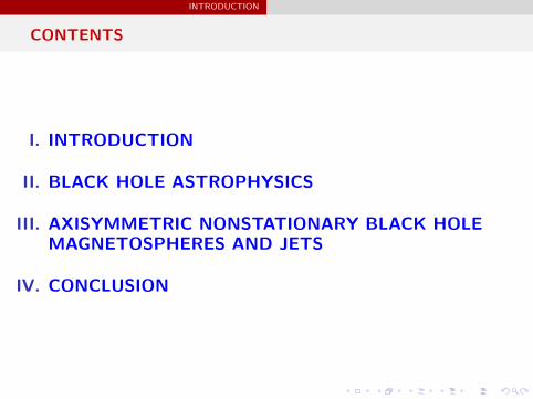
INTRODUCTION
CONTENTS
I. INTRODUCTION
II. BLACK HOLE ASTROPHYSICS
III. AXISYMMETRIC NONSTATIONARY BLACK HOLEMAGNETOSPHERES AND JETS
IV. CONCLUSION

...
.
...
.
...
.
...
.
...
.
...
.
...
.
...
.
...
.
...
.
INTRODUCTION
IINTRODUCTION

...
.
...
.
...
.
...
.
...
.
...
.
...
.
...
.
...
.
...
.
INTRODUCTION
I. INTRODUCTION
Black Hole Astrophysics−→ Black Hole Thermodynamics−→ Black Hole Electrodynamics
−→ Black Hole Magnetospheres & Jets−→ Axisymmetric, Stationary Cases−→ Axisymmetric, Nonstationary Cases

...
.
...
.
...
.
...
.
...
.
...
.
...
.
...
.
...
.
...
.
BLACK HOLE ASTROPHYSICS
IIBLACK HOLE ASTROPHYSICS

...
.
...
.
...
.
...
.
...
.
...
.
...
.
...
.
...
.
...
.
BLACK HOLE ASTROPHYSICS
II. BLACK HOLE ASTROPHYSICS I
In cylindrical coordinates (ϖ,φ, z),
Electric Field : E = Eϖeϖ + Eφeφ + Ezez
Magnetic Field : B = Bϖeϖ +Bφeφ +Bzez
Toroidal Components : ET = Eφeφ and BT = Bφeφ
Poloidal Components : EP = Eϖeϖ + Ezez and BP = Bϖeϖ +Bzez
where ϖ is the perpendicular distance separating the symmetry axis of anarbitrary FIDO (Fiducial Observer) and (eϖ, eφ, ez) are orthonormal unitvectors. (In Newtonian case, ϖ → R)

...
.
...
.
...
.
...
.
...
.
...
.
...
.
...
.
...
.
...
.
BLACK HOLE ASTROPHYSICS
II. BLACK HOLE ASTROPHYSICS II
In cylindrical coordinates (ϖ,φ, z),
Axisymmetric Conditions : ∂f∂φ = 0 and ∂f
∂φ = 0
Stationary Conditions : ∂f∂t = 0 and ∂f
∂t = 0
Nonstationary Conditions : ∂f∂t = 0 and ∂f
∂t = 0
f and f : any scalar and vector, resp..

...
.
...
.
...
.
...
.
...
.
...
.
...
.
...
.
...
.
...
.
BLACK HOLE ASTROPHYSICS
II. BLACK HOLE ASTROPHYSICS III
We assume that the following highly conducting plasma condition issatisfied everywhere :
E +1
cvF × B ≃ 0 , (2.1)
while the force-free condition
ρeE +1
cj × B ≃ 0 (2.2)
is satisfied only in Region 1 (i.e., Relativistic).

...
.
...
.
...
.
...
.
...
.
...
.
...
.
...
.
...
.
...
.
BLACK HOLE ASTROPHYSICS
II. BLACK HOLE ASTROPHYSICS IV
The cross section of an active galactic nucleus (AGN).
...
.
...
.
...
.
...
.
...
.
...
.
...
.
...
.
...
.
...
.
BLACK HOLE ASTROPHYSICS
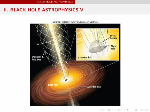
II. BLACK HOLE ASTROPHYSICS V
(Source: Internet Encyclopedia of Science)

...
.
...
.
...
.
...
.
...
.
...
.
...
.
...
.
...
.
...
.
BLACK HOLE ASTROPHYSICS
II. BLACK HOLE ASTROPHYSICS VI
Let us consider a FIDO (Fiducial Observer) that is fixed at a given pointnear a Kerr black hole. In this case, Maxwell’s equations, which satisfy theaxisymmetric condition, can be written as follows:
∇ · E = 4πρe, (2.3)∇ · B = 0, (2.4)
∇× (αE) = −1
c
[∂B∂t
− (B · ∇ω)m], (2.5)
and∇× (αB) =
1
c
[∂E∂t
− (E · ∇ω)m]+
4παjc
. (2.6)
...
.
...
.
...
.
...
.
...
.
...
.
...
.
...
.
...
.
...
.
BLACK HOLE ASTROPHYSICS
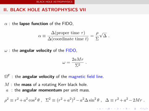
II. BLACK HOLE ASTROPHYSICS VII
α : the lapse function of the FIDO,
α ≡ ∆(proper time τ)
∆(coordinate time t)=
ρ
Σ
√∆ .
ω : the angular velocity of the FIDO,
ω =2aMr
Σ2.
ΩF : the angular velocity of the magnetic field line.M : the mass of a rotating Kerr black hole.a : the angular momentum per unit mass.
ρ2 ≡ r2+a2 cos2 θ , Σ2 ≡ (r2+a2)2−a2∆ sin2 θ , ∆ ≡ r2+a2−2Mr .

...
.
...
.
...
.
...
.
...
.
...
.
...
.
...
.
...
.
...
.
BLACK HOLE ASTROPHYSICS
II. BLACK HOLE ASTROPHYSICS VIII
Define an m-loop ∂A, and any surface A bounded by ∂A which is notintersecting the event horizon of the black hole.
We also define the outward normal vector dS of an infinitesimal area on A.
Define :I : the total electric current passing downward through A,Ψ : the total magnetic flux passing upward through AΦ : the total electric flux passing upward through A

...
.
...
.
...
.
...
.
...
.
...
.
...
.
...
.
...
.
...
.
BLACK HOLE ASTROPHYSICS
II. BLACK HOLE ASTROPHYSICS IX
Investigated by Macdonald & Thorne (1982, MT).

...
.
...
.
...
.
...
.
...
.
...
.
...
.
...
.
...
.
...
.
BLACK HOLE ASTROPHYSICS
II. BLACK HOLE ASTROPHYSICS X
Region 1The Stationary, Relativistic Grad-Shafranov Equation[Macdonald & Thorne 1982]
∇ ·
[α
ϖ2
1−
(ω − ΩF
αcϖ
)2∇Ψ
]− ω − ΩF
αc2∇ΩF · ∇Ψ
+16π2I
αc2ϖ2
dI
dΨ= 0 (2.7)
The Grad-Shafranov Equation : A second-order, non-linear partialdifferential equation that describes the relationship between the plasmaflow distribution and pressure in terms of magnetic flux function Ψ.

...
.
...
.
...
.
...
.
...
.
...
.
...
.
...
.
...
.
...
.
BLACK HOLE ASTROPHYSICS
II. BLACK HOLE ASTROPHYSICS XI
Investigated by Park & Vishniac (1989, PV).

...
.
...
.
...
.
...
.
...
.
...
.
...
.
...
.
...
.
...
.
BLACK HOLE ASTROPHYSICS
II. BLACK HOLE ASTROPHYSICS XII
Axisymmetric, Axisymmetric,Stationary Nonstationary
Electric Current I(r) ≡ −∫Aαj · dS I(t, r) ≡ −
∫Aαj · dS
Magnetic Flux Ψ(r) ≡∫A
B · dS Ψ(t, r) ≡∫A
B · dS
Electric Flux Φ(r) ≡∫A
E · dS Φ(t, r) ≡∫A
E · dS
Electric Field (Toroidal) ET = 0 ET = − 2αϖ
(Ψ4π
)eφ
Magnetic Field (Toroidal) BT = − 2Iαϖ
eφ BT = − 2αϖ
(I − Φ
4π
)eφ
Electric Field (Poloidal) EP =∇Φ×eφ
2πϖEP = EP
Magnetic Field (Poloidal) BP =∇Ψ×eφ
2πϖBP =
∇Ψ×eφ
2πϖ

...
.
...
.
...
.
...
.
...
.
...
.
...
.
...
.
...
.
...
.
BLACK HOLE ASTROPHYSICS
II. BLACK HOLE ASTROPHYSICS XIII
Region 1Based on PV model, Song & Park induced the nonstationary, relativisticGrad-Shafranov Equation. [Song & Park 2016]
∇ ·
[α
ϖ2
1−
(ω − ΩF
αcϖ
)2∇Ψ
]− ω − ΩF
αc2∇ΩF · ∇Ψ
+4πϖ
α2c3ϖ
(I − Φ
4π
)∂ΩF∂z
+4π
c3∂
∂z
[ϖ
αϖ
ω − ΩFα
(I − Φ
4π
)]
+1
αc2ϖ2
[(α
α+
ϖ
ϖ
)Ψ− Ψ
]+
φ
c2ϖ
ω − ΩFα
∂Ψ
∂ϖ
−16π2ξ
c2ϖ2
(I − Φ
4π
)= 0 (2.8)

...
.
...
.
...
.
...
.
...
.
...
.
...
.
...
.
...
.
...
.
BLACK HOLE ASTROPHYSICS
II. BLACK HOLE ASTROPHYSICS XIV
Region 2The Stationary, Newtonian Grad-Shafranov Equation(by setting α = 1, ω = 0, and ϖ = R in (2.7))[Goldreich & Julian 1969]
∇·
[1
R2
1−
(RΩFc
)2∇Ψ
]+ΩFc2
∇ΩF ·∇Ψ+16π2I
c2R2
dI
dΨ= 0 (2.9)
−→ The so-called “Pulsar Equation” investigated by Goldreich & Julian.
...
.
...
.
...
.
...
.
...
.
...
.
...
.
...
.
...
.
...
.
BLACK HOLE ASTROPHYSICS
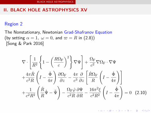
II. BLACK HOLE ASTROPHYSICS XV
Region 2The Nonstationary, Newtonian Grad-Shafranov Equation(by setting α = 1, ω = 0, and ϖ = R in (2.8))[Song & Park 2016]
∇ ·
[1
R2
1−
(RΩFc
)2∇Ψ
]+
ΩFc2
∇ΩF · ∇Ψ
+4πR
c3R
(I − Φ
4π
)∂ΩF∂z
− 4π
c3∂
∂z
[RΩFR
(I − Φ
4π
)]
+1
c2R2
(R
RΨ− Ψ
)− ΩFφ
c2R
∂Ψ
∂R− 16π2ξ
c2R2
(I − Φ
4π
)= 0 (2.10)
...
.
...
.
...
.
...
.
...
.
...
.
...
.
...
.
...
.
...
.
BLACK HOLE ASTROPHYSICS
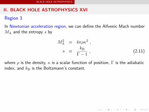
II. BLACK HOLE ASTROPHYSICS XVI
Region 3In Newtonian acceleration region, we can define the Alfvenic Mach numberMA and the entropy s by
M2A ≡ 4πρκ2 ,
s ≡ kBΓ− 1
, (2.11)
where ρ is the density, κ is a scalar function of position, Γ is the adiabaticindex, and kB is the Boltzmann’s constant.
...
.
...
.
...
.
...
.
...
.
...
.
...
.
...
.
...
.
...
.
BLACK HOLE ASTROPHYSICS
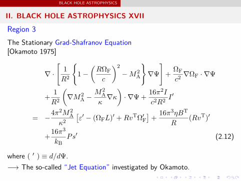
II. BLACK HOLE ASTROPHYSICS XVII
Region 3The Stationary Grad-Shafranov Equation[Okamoto 1975]
∇ ·
[1
R2
1−
(RΩFc
)2
−M2A
∇Ψ
]+
ΩFc2
∇ΩF · ∇Ψ
+1
R2
(∇M2
A −M2
Aκ
∇κ
)· ∇Ψ+
16π2I
c2R2I ′
= −4π2M2
Aκ2
[ε′ − (ΩFL)
′ +RvTΩ′F]+
16π3ηBT
R(RvT)′
+16π3
kBPs′ (2.12)
where ( ′ ) ≡ d/dΨ.−→ The so-called “Jet Equation” investigated by Okamoto.

...
.
...
.
...
.
...
.
...
.
...
.
...
.
...
.
...
.
...
.
BLACK HOLE ASTROPHYSICS
II. BLACK HOLE ASTROPHYSICS XVIII
Region 3The Nonstationary Grad-Shafranov Equation[Song & Park 2016]
∇ ·[
1
R2
1 −
(RΩF
c
)2
− M2A −
R2ΩFC
c2
∂Ψ
∂z
∇Ψ
]+
ΩF − C
c2∇ΩF · ∇Ψ
+1
R2
(∇M
2A −
M2Aκ
∇κ
)· ∇Ψ +
1
c2R2∇(R
2ΩFC
∂Ψ
∂z
)· ∇Ψ −
2ΩFC
c2R
∂Ψ
∂R
+1
c2R2
(R
RΨ − Ψ − RΩFφ
∂Ψ
∂R
)−
4π
c3R
(ΩF + C
) ∂
∂z
[R
(I −
Φ
4π
)]+
16π2
c2R2 |∇Ψ|2
(I −
Φ
4π
)∇I · ∇Ψ
= −4π2M2
Aκ2 |∇Ψ|2
[∇ε − ∇(ΩFL) + Rv
T∇ΩF +2κ
cR2
(I −
Φ
4π
)∇(Rv
T)
]· ∇Ψ
+4π2M2
AkBρκ2 |∇Ψ|2
[P ∇s + s ∇P −
kBP
ρ
(1 +
s
kB
)∇ρ
]· ∇Ψ
−4π2M2
Aκ2 |∇Ψ|2
[1
ρ(vR − v
Tφ)
∂Ψ
∂R+
vz
ρ
∂Ψ
∂z+ |∇Ψ| H
](2.13)
...
.
...
.
...
.
...
.
...
.
...
.
...
.
...
.
...
.
...
.
BLACK HOLE ASTROPHYSICS
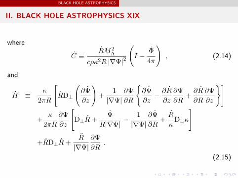
II. BLACK HOLE ASTROPHYSICS XIX
where
C ≡RM2
Acρκ2R |∇Ψ|2
(I − Φ
4π
), (2.14)
and
H ≡ κ
2πR
[RD⊥
(∂Ψ
∂z
)+
1
|∇Ψ|∂Ψ
∂R
∂Ψ
∂z− ∂R
∂z
∂Ψ
∂R+
∂R
∂R
∂Ψ
∂z
]
+κ
2πR
∂Ψ
∂z
[D⊥R+
Ψ
R|∇Ψ|− 1
|∇Ψ|∂Ψ
∂R+
R
κD⊥κ
]
+RD⊥R+R
|∇Ψ|∂Ψ
∂R.
(2.15)

...
.
...
.
...
.
...
.
...
.
...
.
...
.
...
.
...
.
...
.
BLACK HOLE ASTROPHYSICS
II. BLACK HOLE ASTROPHYSICS XVI
The TheRegions Physics Stationary Nonstationary
GSEs GSEs0 < α < 1,
Region 1 0 < ω < ΩH, (2.7) (2.8)M2
A = 0, s = 0
ϖ = RRegion 2 α = 1, ω = 0, (2.9) (2.10)
M2A = 0, s = 0
ϖ = RRegion 3 α = 1, ω = 0, (2.12) (2.13)
M2A = 0, s = 0
Table: The Grad-Shafranov Equations (GSEs)

...
.
...
.
...
.
...
.
...
.
...
.
...
.
...
.
...
.
...
.
CONCLUSION
IVCONCLUSION

...
.
...
.
...
.
...
.
...
.
...
.
...
.
...
.
...
.
...
.
CONCLUSION
IV. CONCLUSION I
Evidently, there are many nonstationary phenomena beyond the scope ofmy paper that can play important roles in a reallistic picture of a blackhole magnetosphere.
It is unfortunate that the GSEs for the nonstationary case in Regions 1, 2,and 3, (2.8), (2.10), and (2.13), seem to be too complicated to solvedirectly via analytic methods. If we can solve these GSEs numerically, thenwe will understand the axisymmetric, nonstationary black holemagnetosphere in more rigorous ways.
My future work may include the luminosity variability, the precession of thecentral black holes, the formation of the nodes in the middle of theastrophysical jets, and so on.

...
.
...
.
...
.
...
.
...
.
...
.
...
.
...
.
...
.
...
.
CONCLUSION
Goldreich, P., & Julian, W. H. 1969, ApJ, 157, 869
Lovelace, R. V. E., Mehanian, C., Mobarry, C. M., & Sulkanen, M. E.1986, ApJS, 62, 1Macdonald, D. A., & Thorne, K. S. 1982, MNRAS, 198, 345
Okamoto, I. 1975, MNRAS, 173, 357
Song, Y. G., & Park, S. J. 2016, ApJ, in press.

...
.
...
.
...
.
...
.
...
.
...
.
...
.
...
.
...
.
...
.
CONCLUSION
Thank You!

...
.
...
.
...
.
...
.
...
.
...
.
...
.
...
.
...
.
...
.
CONCLUSION
The Lapse Function
For non-inertial observers, and in general relativity, coordinate systems canbe chosen more freely. For a clock whose spatial coordinates are constant,the relationship between proper time τ and coordinate time t, i.e. therate of time dilation, is given by
dτ
dt=
√−g00
where g00 is a component of the metric tensor, which incorporatesgravitational time dilation (under the convention that the zerothcomponent is timelike).
...
.
...
.
...
.
...
.
...
.
...
.
...
.
...
.
...
.
...
.
CONCLUSION
Coordinate Time
In the theory of relativity, it is convenient to express results in terms of aspacetime coordinate system relative to an implied observer. In many (butnot all) coordinate systems, an event is specified by one time coordinateand three spatial coordinates. The time specified by the time coordinate isreferred to as coordinate time to distinguish it from proper time.

...
.
...
.
...
.
...
.
...
.
...
.
...
.
...
.
...
.
...
.
CONCLUSION
Proper Time
In relativity, proper time along a timelike world line is defined as the timeas measured by a clock following that line. It is thus independent ofcoordinates, and a Lorentz scalar. This is the quantity of interest, sinceproper time itself is fixed only up to an arbitrary additive constant, namelythe setting of the clock at some event along the world line. The propertime between two events depends not only on the events but also theworld line connecting them, and hence on the motion of the clock betweenthe events. It is expressed as an integral over the world line. Anaccelerated clock will measure a smaller elapsed time between two eventsthan that measured by a non-accelerated (inertial) clock between the sametwo events. The twin paradox is an example of this effect.

...
.
...
.
...
.
...
.
...
.
...
.
...
.
...
.
...
.
...
.
CONCLUSION
Force Free Condition
A force-free magnetic field is a magnetic field that arises when the plasmapressure is so small, relative to the magnetic pressure, that the plasmapressure may be ignored, and so only the magnetic pressure is considered.For a force free field, the electric current density is either zero or parallel tothe magnetic field. The name ”force-free” comes from being able toneglect the force from the plasma.