The Government and Fiscal Policy 9 - pogodzinski.netpogodzinski.net/Macro/ECON_1A_Chapter_9.pdf · aggregate expenditure function is the new ... function up by 50. As Y rises in response,

1 of 40 © 2014 Pearson Education, Inc.

CHAPTER OUTLINE 9 The Government and

Fiscal Policy Government in the Economy Government Purchases (G), Net Taxes (T), and Disposable Income (Yd) The Determination of Equilibrium Output (Income)

Fiscal Policy at Work: Multiplier Effects The Government Spending Multiplier The Tax Multiplier The Balanced-Budget Multiplier

The Federal Budget The Budget in 2012 Fiscal Policy Since 1993: The Clinton, Bush, and Obama Administrations The Federal Government Debt

The Economy’s Influence on the Government Budget Automatic Stabilizers and Destabilizers Full-Employment Budget

Looking Ahead

Appendix A: Deriving the Fiscal Policy Multipliers

Appendix B: The Case in Which Tax Revenues Depend on Income


fiscal policy The government’s spending and taxing policies.

monetary policy The behavior of the Federal Reserve concerning the nation’s money supply.


discretionary fiscal policy Changes in taxes or spending that are the result of deliberate changes in government policy.

net taxes (T) Taxes paid by firms and households to the government minus transfer payments made to households by the government.

disposable, or after-tax, income (Yd) Total income minus net taxes: Y − T.

disposable income ≡ total income − net taxes

Yd ≡ Y − T

Government in the Economy

Government Purchases (G), Net Taxes (T), and Disposable Income (Yd)


� FIGURE 9.1 Adding Net Taxes (T) and Government Purchases (G) to the Circular Flow of Income


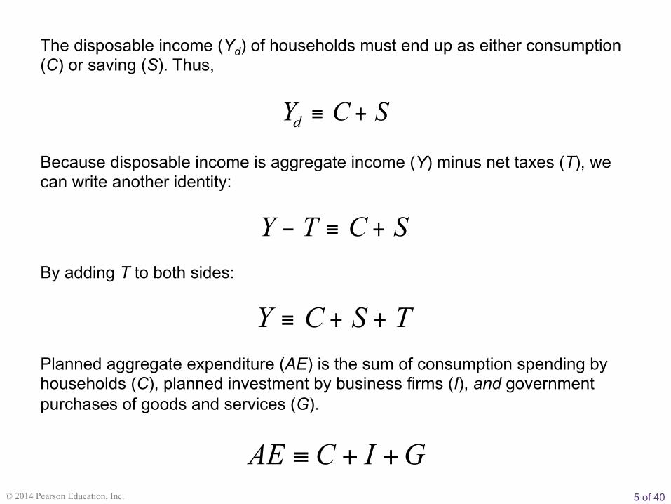
The disposable income (Yd) of households must end up as either consumption (C) or saving (S). Thus,

Y C Sd ≡ +

Y T C S− ≡ +

Y C S T≡ + +

Because disposable income is aggregate income (Y) minus net taxes (T), we can write another identity:

By adding T to both sides:

Planned aggregate expenditure (AE) is the sum of consumption spending by households (C), planned investment by business firms (I), and government purchases of goods and services (G).

GICAE ++≡


budget deficit The difference between what a government spends and what it collects in taxes in a given period: G − T.

budget deficit ≡ G − T

To modify our aggregate consumption function to incorporate disposable income instead of before-tax income, instead of C = a + bY, we write

C = a + bYd or

C = a + b(Y − T)

Our consumption function now has consumption depending on disposable income instead of before-tax income.

Adding Taxes to the Consumption Function


The government can affect investment behavior through its tax treatment of depreciation and other tax policies.

Planned investment depends on the interest rate, both of which we continue to assume are fixed for purposes of this chapter.

Planned Investment


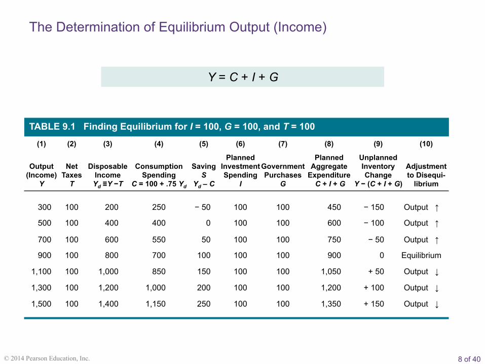
Y = C + I + G

TABLE 9.1 Finding Equilibrium for I = 100, G = 100, and T = 100

(1) (2) (3) (4) (5) (6) (7) (8) (9) (10)

Output

(Income) Y

Net

Taxes T

Disposable

Income Yd ≡Y −T

Consumption

Spending C = 100 + .75 Yd

Saving

S Yd – C

Planned Investment Spending

I

Government Purchases

G

Planned Aggregate

Expenditure C + I + G

Unplanned Inventory Change

Y − (C + I + G)

Adjustment to Disequi-

librium

300 100 200 250 − 50 100 100 450 − 150 Output ↑

500 100 400 400 0 100 100 600 − 100 Output ↑

700 100 600 550 50 100 100 750 − 50 Output ↑

900 100 800 700 100 100 100 900 0 Equilibrium

1,100 100 1,000 850 150 100 100 1,050 + 50 Output ↓

1,300 100 1,200 1,000 200 100 100 1,200 + 100 Output ↓

1,500 100 1,400 1,150 250 100 100 1,350 + 150 Output ↓

The Determination of Equilibrium Output (Income)


� FIGURE 9.2 Finding Equilibrium Output/Income Graphically

Because G and I are both fixed at 100, the aggregate expenditure function is the new consumption function displaced upward by I + G = 200.

Equilibrium occurs at Y = C + I + G = 900.


saving/investment approach to equilibrium:

S + T = I + G

To derive this, we know that in equilibrium, aggregate output (income) (Y) equals planned aggregate expenditure (AE). By definition, AE equals C + I + G, and by definition, Y equals C + S + T. Therefore, at equilibrium:

C + S + T = C + I + G

Subtracting C from both sides leaves:

S + T = I + G

The Saving/Investment Approach to Equilibrium


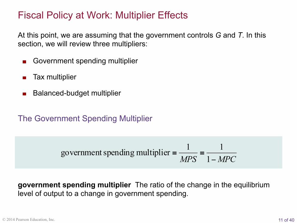
At this point, we are assuming that the government controls G and T. In this section, we will review three multipliers: ! Government spending multiplier

! Tax multiplier

! Balanced-budget multiplier

Fiscal Policy at Work: Multiplier Effects

government spending multiplier The ratio of the change in the equilibrium level of output to a change in government spending.

The Government Spending Multiplier

MPCMPS −≡≡

111multiplier spending government


TABLE 9.2 Finding Equilibrium after a Government Spending Increase of 50 (G Has Increased from 100 in Table 9.1 to 150 Here)

(1) (2) (3) (4) (5) (6) (7) (8) (9) (10)

Output

(Income) Y

Net

Taxes T

Disposable

Income Yd ≡Y −T

Consumption


Saving

S Yd – C


I


G

Planned Aggregate



Y − (C + I + G)

Adjustment

to Disequilibrium

300 100 200 250 - 50 100 150 500 - 200 Output ↑

500 100 400 400 0 100 150 650 - 150 Output ↑

700 100 600 550 50 100 150 800 - 100 Output ↑

900 100 800 700 100 100 150 950 - 50 Output ↑

1,100 100 1,000 850 150 100 150 1,100 0 Equilibrium

1,300 100 1,200 1,000 200 100 150 1,250 + 50 Output ↓


� FIGURE 9.3 The Government Spending Multiplier

Increasing government spending by 50 shifts the AE function up by 50.

As Y rises in response, additional consumption is generated.

Overall, the equilibrium level of Y increases by 200, from 900 to 1,100.


tax multiplier The ratio of change in the equilibrium level of output to a change in taxes.

( )tax multiplier MPC

MPS≡ −

ΔYMPS

= ×⎛⎝⎜

⎞⎠⎟ (initial increase in aggregate expenditure)

1

1( )

MPCY T MPC T

MPS MPSΔ = − Δ × × = −Δ ×⎛ ⎞ ⎛ ⎞

⎜ ⎟ ⎜ ⎟⎝ ⎠ ⎝ ⎠

The Tax Multiplier

Because the initial change in aggregate expenditure caused by a tax change of ∆T is (−∆T × MPC), we can solve for the tax multiplier by substitution:

Because a tax cut will cause an increase in consumption expenditures and output and a tax increase will cause a reduction in consumption expenditures and output, the tax multiplier is a negative multiplier:


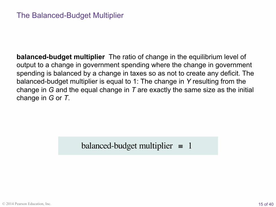
balanced-budget multiplier The ratio of change in the equilibrium level of output to a change in government spending where the change in government spending is balanced by a change in taxes so as not to create any deficit. The balanced-budget multiplier is equal to 1: The change in Y resulting from the change in G and the equal change in T are exactly the same size as the initial change in G or T.

1balanced-budget multiplier ≡

The Balanced-Budget Multiplier


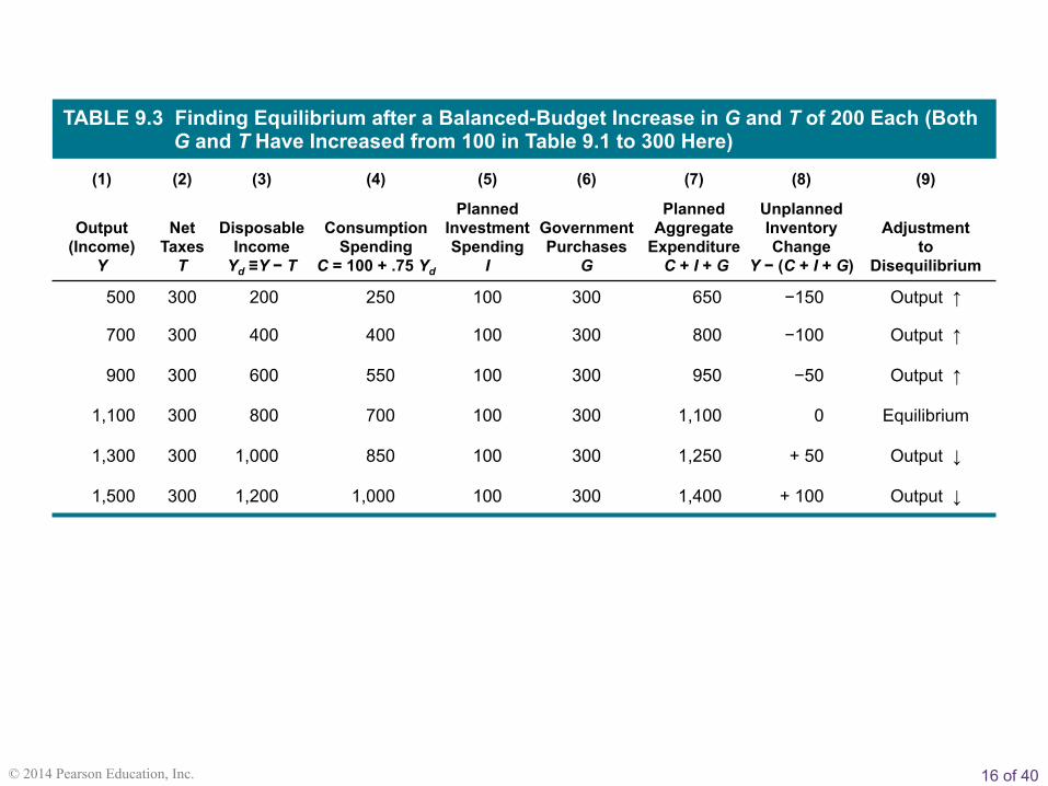
TABLE 9.3 Finding Equilibrium after a Balanced-Budget Increase in G and T of 200 Each (Both G and T Have Increased from 100 in Table 9.1 to 300 Here)

(1) (2) (3) (4) (5) (6) (7) (8) (9)

Output

(Income) Y

Net

Taxes T

Disposable

Income Yd ≡Y − T

Consumption



I


G

Planned Aggregate



Y − (C + I + G)

Adjustment

to Disequilibrium

500 300 200 250 100 300 650 −150 Output ↑

700 300 400 400 100 300 800 −100 Output ↑

900 300 600 550 100 300 950 −50 Output ↑

1,100 300 800 700 100 300 1,100 0 Equilibrium

1,300 300 1,000 850 100 300 1,250 + 50 Output ↓

1,500 300 1,200 1,000 100 300 1,400 + 100 Output ↓


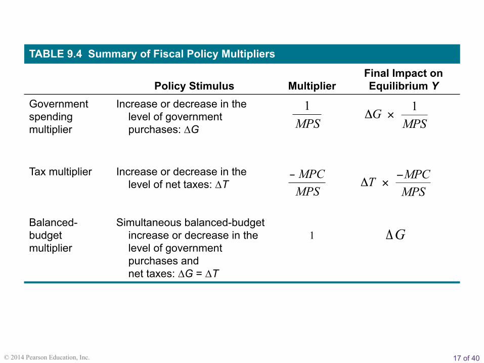
TABLE 9.4 Summary of Fiscal Policy Multipliers

Policy Stimulus

Multiplier

Final Impact on Equilibrium Y

Government spending multiplier

Increase or decrease in the level of government purchases: ∆G

Tax multiplier Increase or decrease in the level of net taxes: ∆T

Balanced-budget multiplier

Simultaneous balanced-budget increase or decrease in the level of government purchases and net taxes: ∆G = ∆T

1

1MPS

− MPCMPS

1 GMPS

Δ ×

MPCTMPS−

Δ ×

ΔG


A Warning

Although we have added government, the story told about the multiplier is still incomplete and oversimplified.

We have been treating net taxes (T) as a lump-sum, fixed amount, whereas in practice, taxes depend on income.

Appendix B to this chapter shows that the size of the multiplier is reduced when we make the more realistic assumption that taxes depend on income.

We continue to add more realism and difficulty to our analysis in the chapters that follow.


federal budget The budget of the federal government.

The Federal Budget

Because fiscal policy is the manipulation of items in the federal budget, that budget is relevant to our study of macroeconomics.

An enormously complicated document up to thousands of pages each year, the federal budget lists in detail all the things the government plans to spend money on and all the sources of government revenues for the coming year.

It is the product of a complex interplay of social, political, and economic forces.


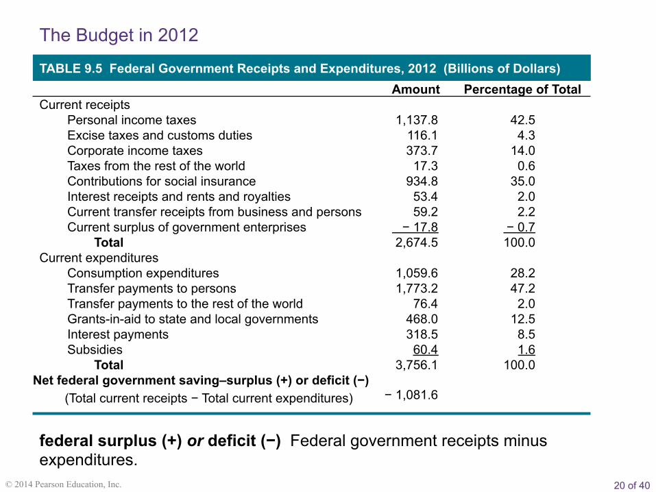
TABLE 9.5 Federal Government Receipts and Expenditures, 2012 (Billions of Dollars) Amount Percentage of Total

Current receipts Personal income taxes 1,137.8 42.5 Excise taxes and customs duties 116.1 4.3 Corporate income taxes 373.7 14.0 Taxes from the rest of the world 17.3 0.6 Contributions for social insurance 934.8 35.0 Interest receipts and rents and royalties 53.4 2.0 Current transfer receipts from business and persons 59.2 2.2 Current surplus of government enterprises − 17.8 − 0.7

Total 2,674.5 100.0 Current expenditures

Consumption expenditures 1,059.6 28.2 Transfer payments to persons 1,773.2 47.2 Transfer payments to the rest of the world 76.4 2.0 Grants-in-aid to state and local governments 468.0 12.5 Interest payments 318.5 8.5 Subsidies 60.4 1.6

Total 3,756.1 100.0 Net federal government saving–surplus (+) or deficit (−) (Total current receipts − Total current expenditures)

− 1,081.6

The Budget in 2012

federal surplus (+) or deficit (−) Federal government receipts minus expenditures.


� FIGURE 9.4 Federal Personal Income Taxes as a Percentage of Taxable Income, 1993 I–2012 IV

Fiscal Policy Since 1993: The Clinton, Bush, and Obama Administrations


� FIGURE 9.5 Federal Government Consumption Expenditures as a Percentage of GDP and Federal Transfer Payments and Grants-in-Aid as a Percentage of GDP, 1993 I–2012 IV


� FIGURE 9.6 The Federal Government Surplus (+) or Deficit (−) as a Percentage of GDP, 1993 I–2012 IV


federal debt The total amount owed by the federal government.

privately held federal debt The privately held (non-government-owned) debt of the U.S. government.

The Federal Government Debt


� FIGURE 9.7 The Federal Government Debt as a Percentage of GDP, 1993 I–2012 IV


automatic stabilizers Revenue and expenditure items in the federal budget that automatically change with the state of the economy in such a way as to stabilize GDP.

fiscal drag The negative effect on the economy that occurs when average tax rates increase because taxpayers have moved into higher income brackets during an expansion.

The Economy’s Influence on the Government Budget

Automatic Stabilizers and Destabilizers

automatic destabilizer Revenue and expenditure items in the federal budget that automatically change with the state of the economy in such a way as to destabilize GDP.


full-employment budget What the federal budget would be if the economy were producing at the full-employment level of output.

structural deficit The deficit that remains at full employment.

cyclical deficit The deficit that occurs because of a downturn in the business cycle.

Full-Employment Budget


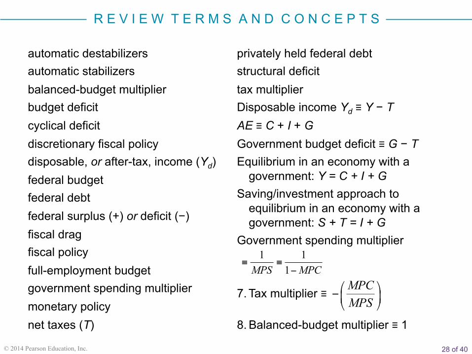
automatic destabilizers automatic stabilizers balanced-budget multiplier budget deficit cyclical deficit discretionary fiscal policy disposable, or after-tax, income (Yd) federal budget federal debt federal surplus (+) or deficit (−) fiscal drag fiscal policy full-employment budget government spending multiplier monetary policy net taxes (T)

privately held federal debt structural deficit tax multiplier Disposable income Yd ≡ Y − T AE ≡ C + I + G Government budget deficit ≡ G − T Equilibrium in an economy with a

government: Y = C + I + G Saving/investment approach to

equilibrium in an economy with a government: S + T = I + G

Government spending multiplier

7. Tax multiplier ≡

8. Balanced-budget multiplier ≡ 1

MPCMPS

⎛ ⎞−⎜ ⎟⎝ ⎠

MPCMPS −≡≡111

R E V I E W T E R M S A N D C O N C E P T S


Y C I G= + +

C a b Y T= + −( )

Y a b Y T I G= + − + +( )Y a bY bT I G= + − + +

Y bY a I G bT− = + + −Y b a I G bT( )1− = + + −

( ))(

11 bTGIa

b Y −++

−=

CHAPTER 9 APPENDIX A Deriving the Fiscal Policy Multipliers The Government Spending and Tax Multipliers

We can derive the multiplier algebraically using our hypothetical consumption function:

The equilibrium condition is

By substituting for C, we get

This equation can be rearranged to yield

Now solve for Y by dividing through by (1 − b):


It is easy to show formally that the balanced-budget multiplier = 1.

GΔinitial increase in spending: ( )C T MPCΔ = Δ− initial decrease in spending: ( )G T MPCΔ −Δ= net initial increase in spending

In a balanced-budget increase, ∆G = ∆T; so in the above equation for the net initial increase in spending we can substitute ∆G for ∆T.

∆G − ∆G (MPC) = ∆G (1 − MPC)

The Balanced-Budget Multiplier


1( )Y G MPS GMPS

⎛ ⎞Δ = Δ = Δ⎜ ⎟⎝ ⎠

Because MPS = (1 − MPC), the net initial increase in spending is:

∆G (MPS)

We can now apply the expenditure multiplier to this net initial increase in spending:

⎟⎠

⎞⎜⎝

⎛MPS1

Thus, the final total increase in the equilibrium level of Y is just equal to the initial balanced increase in G and T.


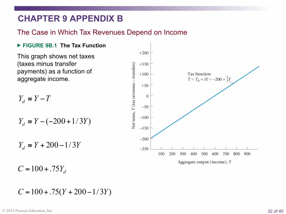
TYYd −≡

)3/1200( YYYd +−−≡

YYYd 3/1200−+≡

dYC 75.100+=

)3/1200(75.100 YYC −++=

� FIGURE 9B.1 The Tax Function

CHAPTER 9 APPENDIX B The Case in Which Tax Revenues Depend on Income

This graph shows net taxes (taxes minus transfer payments) as a function of aggregate income.


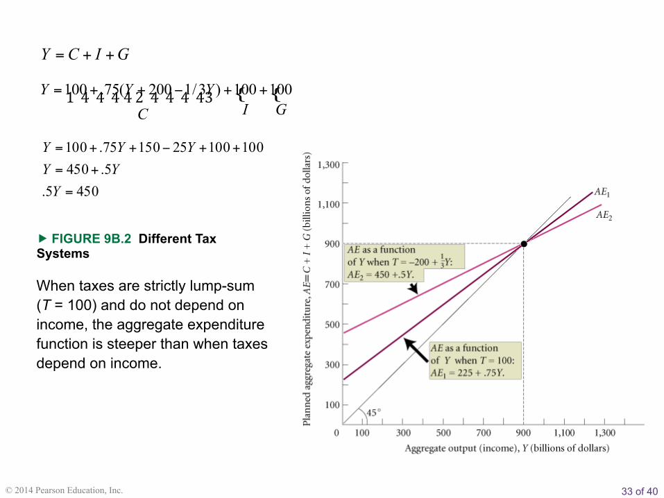
When taxes are strictly lump-sum (T = 100) and do not depend on income, the aggregate expenditure function is steeper than when taxes depend on income.

� FIGURE 9B.2 Different Tax Systems

GICY ++=

{ {100 .75( 200 1/3 ) 100 100Y Y YI GC

= + + − + +1 4 4 4 4 2 4 4 4 43

4505.5.450

1001002515075.100

=

+=

++−++=

YYY

YYY


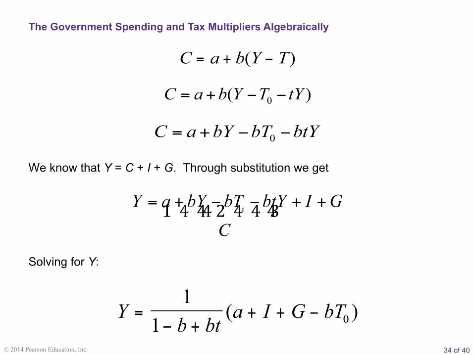
C a b Y T= + −( )

0C a bY bT btY= + − −

0( )C a b Y T tY= + − −

0Y a bY bT btY I G

C= + − − + +1 4 44 2 4 4 43

Yb bt

a I G bT=− +

+ + −1

1 0( )

The Government Spending and Tax Multipliers Algebraically

We know that Y = C + I + G. Through substitution we get

Solving for Y:


11 b bt− +

This means that a $1 increase in G or I (holding a and T0 constant) will increase the equilibrium level of Y by

Holding a, I, and G constant, a fixed or lump-sum tax cut (a cut in T0) will increase the equilibrium level of income by

btbb+−1

Documents

The Government and Fiscal Policy 9 - pogodzinski.netpogodzinski.net/Macro/ECON_1A_Chapter_9.pdf · aggregate expenditure function is the new ... function up by 50. As Y rises in response,