Embed Size (px)
Citation preview
MPIDR WORKING PAPER WP 2012-008FEBRUARY 2012
Adam Lenart ([email protected])
The Gompertz distribution and Maximum Likelihood Estimation of its parameters - a revision
Max-Planck-Institut für demografi sche ForschungMax Planck Institute for Demographic ResearchKonrad-Zuse-Strasse 1 · D-18057 Rostock · GERMANYTel +49 (0) 3 81 20 81 - 0; Fax +49 (0) 3 81 20 81 - 202; http://www.demogr.mpg.de
This working paper has been approved for release by: James W. Vaupel ([email protected]),Head of the Laboratory of Survival and Longevity and Head of the Laboratory of Evolutionary Biodemography.
© Copyright is held by the authors.
Working papers of the Max Planck Institute for Demographic Research receive only limited review.Views or opinions expressed in working papers are attributable to the authors and do not necessarily refl ect those of the Institute.
The Gompertz distribution and Maximum LikelihoodEstimation of its parameters - a revision
Adam Lenart
November 28, 2011
Abstract
The Gompertz distribution is widely used to describe the distribution of adultdeaths. Previous works concentrated on formulating approximate relationships to char-acterize it. However, using the generalized integro-exponential function Milgram (1985)exact formulas can be derived for its moment-generating function and central moments.Based on the exact central moments, higher accuracy approximations can be definedfor them. In demographic or actuarial applications, maximum-likelihood estimation isoften used to determine the parameters of the Gompertz distribution. By solving themaximum-likelihood estimates analytically, the dimension of the optimization problemcan be reduced to one both in the case of discrete and continuous data.
Keywords: Gompertz distribution, moment-generating function,expected value, variance, skewness, kurtosis, maximum-likelihoodestimation
1 Introduction
The Gompertz distribution is important in describing the pattern of adult deaths (Wet-terstrand 1981; Gavrilov and Gavrilova 1991). For low levels of infant (and young adult)mortality, the Gompertz force of mortality extends to the whole life span (Vaupel 1986) ofpopulations with no observed mortality deceleration.
The Gompertz distribution has received considerable attention from demographers and ac-tuaries. Pollard and Valkovics (1992) were the first to study the Gompertz distributionthoroughly. However, their results are true only in the case when the initial level of mortal-ity is very close to 0. Kunimura (1998) arrived at similar conclusions. They both definedthe moment generating function of the Gompertz distribution in terms of the incompleteor complete gamma function and their results are either approximate or left in an integralform. Willemse and Koppelaar (2000) reformulated the Gompertz force of mortality andderived relationships for this new formulation. Later, Marshall and Olkin (2007) describedthe negative Gompertz distribution; a Gompertz distribution with a negative rate of agingparameter. Willekens (2002) provided connections between the Gompertz, the Weibull andother Type I extreme value distributions. In this paper, I will keep the most often used
1
formulation of the Gompertz’ law of mortality (Gompertz 1825) in demography (Prestonet al. 2001:9.1). The Gompertz force of mortality at age x, x ≥ 0, is
µ(x) = aebx a, b > 0 , (1)
where a denotes the level of the force of mortality at age 0 and b the rate of aging. Themoments of the Gompertz distribution can be explicitly given by the generalized integro-exponential function (Milgram 1985), that offers exact power series representation of them.
2 The Gompertz distribution
The Gompertz distribution has a continuous probability density function with location pa-rameter a and shape parameter b,
f(x) = aebx−ab (ebx−1) , (2)
with support on (−∞,∞). In actuarial or demographic applications, x usually denotes agewhich cannot be negative, leading to bounded support on [0,∞). The truncated distributionyields a proper density function by rescaling the a parameter to correspond to x = 0 (Garget al. 1970). The distribution function is
F (x) = 1− e−ab (ebx−1) .
The moment generating function of the Gompertz distribution is given by its Laplace trans-form.
Proposition 1. The Laplace transform of the Gompertz distribution is
L(s) =a
be
abE s
b
(ab
)a, b > 0 , (3)
where En(z) =∞∫1
e−zt
tndt (Abramowitz and Stegun 1965:5.1.4).
Proof. The Laplace transform of the Gompetz pdf of (2) is
L(s) =
∞∫0
aebx−ab (ebx−1)e−sx dx . (4)
By substituting q = ebx in (4)
L(s) =a
be
ab
∞∫1
e−abqq−
sb dq
2
Note that the exponential integral, En(z), is defined as (Abramowitz and Stegun 1965:5.1.4)
En(z) =
∞∫1
e−zt
tndt n > 0, Re(z) > 0 ,
therefore
L(s) =a
be
abE s
b
(ab
)
The moments of the Gompertz distribution are expressed as the derivatives of its Laplacetransform that can be expressed in a general formula by using the generalized integro-exponential function (Milgram 1985).
Proposition 2. The nth moment of a Gompertz distributed random variable X is
E [Xn] =n!
bne
abEn−1
1
(ab
), (5)
where Ens (z) = 1
n!
∞∫1
(lnx)nx−se−zx dz is the generalized integro-exponential function (Milgram
1985).
Proof. The moments of random variable X of a Gompertz distribution can be calculatedwith the aid of the Laplace transform. From (3),
E [X] = − d
dsL(s)
∣∣∣∣s=0
=a
be
ab
∞∫1
1
be−
abx ln(x) dx
E[X2]
=d2
ds2L(s)
∣∣∣∣s=0
=a
be
ab
∞∫1
1
b2e−
abx[ln(x)]2 dx
...
E [Xn] = (−1)n+1 dn
dsnL(s)
∣∣∣∣s=0
=a
be
ab
∞∫1
1
bne−
abx[ln(x)]n dx
By integration by parts
E [Xn] = eab
∞∫1
n
bnx−1e−
abx[ln(x)]n−1 dx
3
Note that the intergral representation of the generalized integro-exponential function (Mil-gram 1985) is
Ejs(z) =
1
Γ(j + 1)
∞∫1
[lnx]jx−se−zx dx
or by definition:
Ejs(z) =
(−1)j
j!
∂j
∂sjEs(z) , (6)
and
E0s (z) ≡ Es(z).
Therefore, E [Xn] can be represented by (6):
E [Xn] =n!
bne
abEn−1
1
(ab
)or by the more widely used Meijer G-function (Milgram 1985):
E [Xn] =n!
bne
abGn+1,0
n,n+1
(a
b
∣∣∣∣ ; 1, . . . , 10, . . . , 0;
), (7)
where the Meijer G-function is a generalized hypergeometric function. It is defined by thecontour integral
Gm,np,q
[z
∣∣∣∣ a1, . . . , an; an+1, . . . , apb1, . . . , bm; bm+1, . . . , bq
]=
1
2πi
∫C
m∏j=1
Γ(bj − s)n∏j=1
Γ (1− aj + s)
q∏j=m+1
Γ(1− bj + s)
p∏j=n+1
Γ (aj − s)zs ds
along contour C (Erdelyi 1953).
Series expansion of the integral form offers a simpler, but lengthier, representation of the mo-ments of the Gompertz distribution. The power series expansion of the generalized integro-exponential function (Milgram 1985:2.10) in the Gompertz case, ie. for s = 1 and z = a
b
is,
En−11
(ab
)=
[∞∑j=1
1
(−j)n(−a
b)j
j!
]+
(−1)n
n!
n∑j=0
(n
j
)ln(ab
)n−jΨj , (8)
where
Ψj = limt→0
dj
dtjΓ(1− t) . (9)
4
For j ∈ (0, 1, 2, 3, 4)
Ψ0 = 1 ;
Ψ1 = γ ;
Ψ2 = γ2 +π2
6;
Ψ3 = γ3 + γπ2
2+ 2ζ(3) ;
Ψ4 = γ4 + γ2π2 + 8γζ(3) +3
20π4 ,
where γ ≈ 0.57722 is the Euler-Mascheroni constant and ζ(s) =∞∑n=1
n−s is the Riemann
zeta function (Abramowitz and Stegun 1965:23.2.18). Note that π2
6= ζ(2) and π4
90= ζ(4).
Also note that ζ(3) ≈ 1.2021 is known as Apery’s constant (Apery 1979). Please refer toAppendix A.1 for derivation of the values of the Ψ function.
2.1 Expected value, variance, skewness and kurtosis
Corollary 1. The expected value of random variable X of a Gompertz distribution is
E [X] =1
be
abE1
(ab
)(10)
≈ 1
be
ab
(ab− ln
(ab
)− γ).
The precision of the approximate result depends on the ratio of a to b. For low values of
1be
ab
(ab )
2
4, the approximation is precise.
Proof.
Exact From (5), the expected value of random variable X of a Gompertz distribution, orlife expectancy, is given by
E [X] =1
be
ab
∞∫1
x−1e−abx dx
=1
be
abE1
(ab
)This result has already been shown by Missov and Lenart (2011).
5
Approximate The approximate result for the expected value in a Gompertz model is alsowell-known, when a is close to 0, by Abramowitz and Stegun (1965:5.1.11) the exponentialintegral, E1(z), can be approximated by −γ − ln(z), and (10) appears as 1
be
ab
(−γ − ln a
b
),
where γ = 0.57722 denotes the Euler-Mascheroni constant (see e.g. Pollard and Valkovics1992; Kunimura 1998; Missov and Lenart 2011). However, the precision of the previousapproximations can be improved by adding new terms to it.
From (8) the power series expansion of the expected value is
E [X] =1
be
ab
(−∞∑j=1
(−ab)j
j!−
1∑j=0
(1
j
)ln(ab
)1−jΨj
),
and by (24)
E [X] =1
be
ab
(−∞∑j=1
(−ab)j
j!− ln
(ab
)− γ
).
As a is usually close to 0, ab≈ −
∞∑j=1
(−ab)j
j!and
E [X] ≈ 1
be
ab
(ab− ln
(ab
)− γ). (11)
Note that because the sign of −∞∑j=1
(−ab)j
j!changes, (11) will be slightly overestimated for
relatively large a but by adding new terms of the sum, the expected value, or life expectancyat birth, can be approximated by arbitrary precision. For the error of the approximation,please see Fig. 5 in the Appendix.
Corollary 2. The variance of random variable X of a Gompertz distribution is
V ar [X] =2
b2e
ab
{−ab
3F3
[1, 1, 12, 2, 2;
;a
b
]+
1
2
[π2
6+(γ + ln
(ab
))2]}−[
1
be
abE1
(ab
)]2
(12)
≈ 1
b2π2
6− 2
a
b3.
The approximate result holds for a ≈ 0. pFq
[a1, . . . , apb1, . . . , bq;
; z
]denotes the generalized hyper-
geometric function (e.g. Askey and Daalhuis 2010).
Proof.
Exact The variance of a random variable X is
V ar [X] = E[X2]− E [X]2 .
6
Concentrating on E [X2], if X is Gompertz distributed, from (5):
E[X2]
=2
b2e
abE1
1
(ab
)(13)
An exact representation of (13) can be reached by the G function by (7):
E[X2]
=2
b2e
abG3,0
2,3
(a
b
∣∣∣∣ ; 1, 10, 0, 0;
).
Power series expansion of Ejs yields (Milgram 1985:2.10),
Ej1(z) =
∞∑l=1
1
(−l)j+1
(−z)l
l!+
(−1)j+1
(j + 1)!
j+1∑l=0
(j + 1
l
)ln(z)1+j−lΨl , (14)
where
Ψl = limt→0
dl
dtlΓ(1− t) .
Note that
∞∑l=1
1
(−l)j+1
(−z)l
l!= (−1)jz j+2Fj+2
[11, . . . , 1j+2
21, . . . , 2j+2;; z
],
where pFq
[a1, . . . , apb1, . . . , bq;
; z
]=∞∑k=0
(a1)k···(ap)k
(b1)k···(bp)k
zk
k!denotes the generalized hypergeometric func-
tion (Askey and Daalhuis 2010).
Therefore
E[X2]
=2
b2
{−ab
3F3
[1, 1, 12, 2, 2;
;a
b
]+
1
2
[π2
6+(γ + ln
(ab
))2]}
(15)
and
V ar[X] =2
b2e
ab
{−ab
3F3
[1, 1, 12, 2, 2;
;a
b
]+
1
2
[π2
6+(γ + ln
(ab
))2]}−[
1
be
abE1
(ab
)]2
Approximate By juxtaposing (11) with (15), it is easy to see possible approximations.Pollard and Valkovics (1992) derived that the variance of the Gompertz distribution is 1
b2π2
6.
This result only holds when a is very close to 0. However, from (12), it is clear that thevariance depends on the parameter a, i.e. for fixed b, as a increases, the variance decreases.
When a ≈ 0, by (11)
E[X2]≈ 1
b2e
abπ2
6− e−
abE [X]2
7
and for eab = 1
V ar (X) ≈ 1
b2π2
6. (16)
Note that (16) crudely overestimates the variance for relatively larger a. The value of
3F3
[1, 1, 12, 2, 2;
; ab
]for a ≈ 0 is 1 and for any higher likely values for human force of mortality
(ie. a ≈ 0.1 about age 90), it is equal to about 0.9, or approximately 1. However, −2 ab3
canbe significantly large and is the only term that reduces the overestimated variance of (16) in(12). Therefore,
V ar (X) ≈ 1
b2π2
6− 2
a
b3
always gives a better approximation to the variance than (16). For the error of the approxi-mation, please see Fig. 5 in the Appendix.
Corollary 3. The skewness, γ1 of the probability distribution of random variable X of aGompertz distribution is
γ1 =
6b3e
abG4,0
3,4
(ab
∣∣∣∣ ; 1, 1, 10, 0, 0, 0;
)− 3m1
2b2e
abG3,0
2,3
(ab
∣∣∣∣ ; 1, 10, 0, 0;
)+ 2(m1)
3
(2b2e
ab
{−ab 3F3
[1, 1, 12, 2, 2;
; ab
]+ 1
2
[π2
6+(γ + ln
(ab
))2]}− [1be
abE1
(ab
)]2) 32
≈
{4.15a0.3 − 5b0.49 − 1.48a+ 4.31b− 4.96ab, if a > 0−12√
6π3 ζ(3), if a ≈ 0
,
where m1 denotes the expected value of the distribution.
Proof.
Exact Skewness is given as the third standardized moment,
γ1 =E [X3]− 3E [X]E [X2] + 2E [X]3
V ar [X]32
.
From (7) and (12) the exact result is immediately given. An equivalent power series repre-sentation can be easily acquired from (8) and (9).
Approximate The approximate result is given by the limit of the power series expansionof the third central moment, m3, when a goes to 0
m3|a=0 = lima→0
m3 = − 2
b3ζ(3)
8
and from (16)
γ1|a=0 = lima→0
m3
V ar [X]32
=−12√
6
π3ζ(3) (17)
and for the other cases in the 0 < a, b ≤ 0.2 surface, the approximation is the result of fittingthe
γ1|a>0 ≈ c1ac2 + c3b
c4 + c5a+ c6b+ c7ab
expression by using (unweighted) non-linear least squares. For the error of the approxima-tion, please see Fig. 5 in the Appendix.
Note that (17) also yields the lowest value, γ1 = −1.13955 for the skewness of the Gompertzdistribution.
Corollary 4. The excess kurtosis, γ2 of the probability distribution of random variable X ofa Gompertz distribution is
γ2 =
{24
b4e
abG5,0
4,5
(a
b
∣∣∣∣ ; 1, 1, 1, 10, 0, 0, 0, 0;
)− 4m1
6
b3e
abG4,0
3,4
(a
b
∣∣∣∣ ; 1, 1, 10, 0, 0, 0;
)+6(m1)
2 2
b2e
abG3,0
2,3
(a
b
∣∣∣∣ ; 1, 10, 0, 0;
)+ 3(m1)
4
}/{2
b2e
ab
{−ab
3F3
[1, 1, 12, 2, 2;
;a
b
]+
1
2
[π2
6+(γ + ln
(ab
))2]}−[
1
be
abE1
(ab
)]2}2
− 3
≈
{−0.75 + 34.13a0.253 + 20b0.311 − 53.51(ab)0.14, if a > 0125, if a ≈ 0
,
Proof.
Exact Excess kurtosis is given as the difference between the fourth standardized momentand the kurtosis of the normal distribution; 3,
γ2 =E [X4]− 4E [X]E [X3] + 6E [X]2E [X2]− 3E [X]4
V ar [X]2− 3 .
From (7) and (12) the exact result is immediately given. An equivalent power series repre-sentation can be easily acquired from (8) and (9). Note that the excess kurtosis reaches aminimal value about -0.75.
9
Approximate The approximate result is given by the limit of the power series expansionof the fourth central moment, m4, when a goes to 0
m4|a=0 = lima→0
m4 =3π4
20b4
and from (16)
γ2|a=0 = lima→0
m4
V ar [X]2− 3 =
12
5.
and for the other cases in the 0 < a, b ≤ 0.2 surface, the approximation is the result of fittingthe
γ2|a>0 ≈ −0.75 + c1ac2 + c3b
c4 + c5(ab)c6
expression by using (unweighted) non-linear least squares. For the error of the approxima-tion, please see Fig. 5 in the Appendix.
a
b
0.06
0.08
0.10
0.12
0.14
0.16
0.18
0.20
0.00 0.05 0.10 0.15 0.20
Expected value
75+
50−75
30−50
15−30
10−15
6−10
4−6
2−4
a
b
0.06
0.08
0.10
0.12
0.14
0.16
0.18
0.20
0.00 0.05 0.10 0.15 0.20
Variance
400+
200−400
100−200
50−100
25−50
15−25
10−15
7−10
4−7
a
b
0.06
0.08
0.10
0.12
0.14
0.16
0.18
0.20
0.00 0.05 0.10 0.15 0.20
Skewness
(−1.14)−(−0.5)
(−0.5)−0
0−0.3
0.3−0.5
0.5−0.6
0.6−0.75
0.75−0.85
0.85−1
1+
a
b
0.06
0.08
0.10
0.12
0.14
0.16
0.18
0.20
0.00 0.05 0.10 0.15 0.20
Kurtosis
(−0.75)−(−0.6)
(−0.6)−(−0.3)
(−0.3)−0
0−0.3
0.3−1.5
1.5+
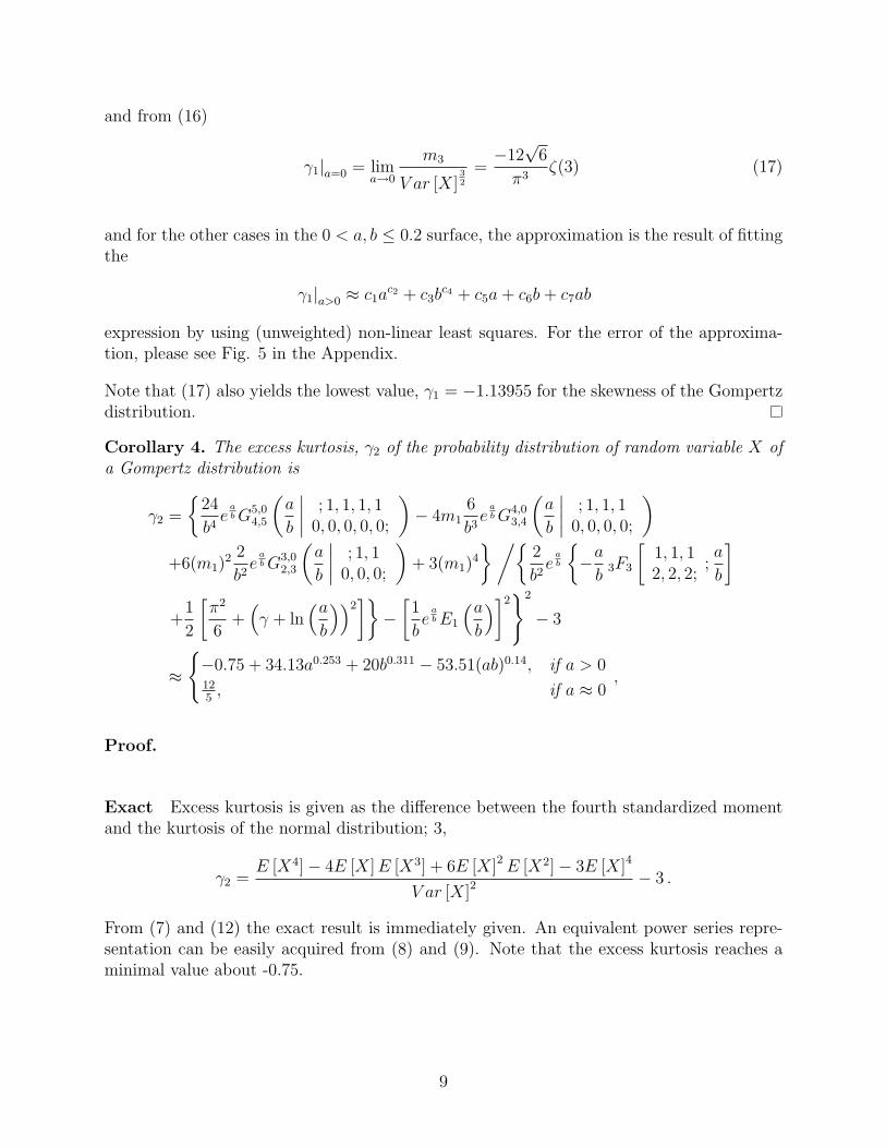
Figure 1: Expected value, variance, skewness and kurtosis of the Gompertz distribution
The Gompertz probability density function can be reformulated into a distribution withlocation and scale parameters. By noting that the mode, M
M =1
bln
(b
a
),
10
(2) can be expressed as
f(x) = bee−bM−eb(x−M)+b(x−M)
3 Maximum Likelihood Estimation
3.1 Discrete age
Often, only discrete data is available and (1) cannot be directly estimated. However, ifthe number of deaths and the number of person-years exposed to the risk of dying can beobserved, we can assume that the number of deaths in a given age interval follows a Poissondistribution.
Let D denote the number of deaths and λ the rate parameter of the Poisson distribution
f(D;λ) =1
D!θDe−λ . (18)
The rate parameter, λ, of the Poisson distribution is consistent with µ(x) as both λ, µ(x) > 0.The rate of occurrence of a Poisson process assumes equal observation window for each unitof observation. When applying the Poisson distribution to death-exposure data, the unitof observation is the number of deaths at each age group, Dx and the observation windowis the number of people (or person-years) who are exposed to the risk of death. Clearly,the number of people at the risk of dying differs from age group to age group. Therefore,θ has to be weighted by the number of person-years exposed to death, Ex at age x. Aftersubstituting λ = λEx in (18) and taking the log of it and eliminating the additive constants,the log-likelihood function of deaths D will be
l(θ|D) ∝∑x
Dx ln θ − Exθ . (19)
If we substitute µ(x) for θ, we assume that we have n independent draws (for each age) froma Poisson distribution with a rate parameter that sheds light on the previously hidden (in(19)) functional relationship between rate λ and age x.
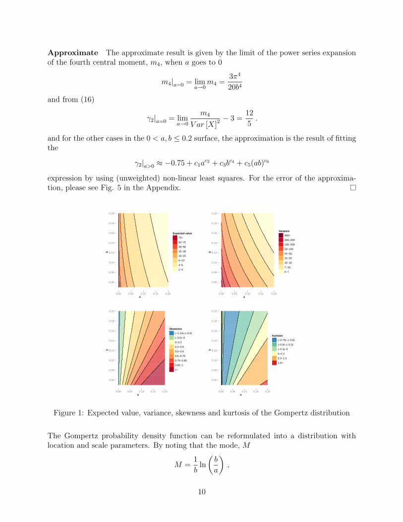
Using data for US females in 2007, aged 35-100 from the Human Mortality Database, pa-rameters a and b can be readily estimated.
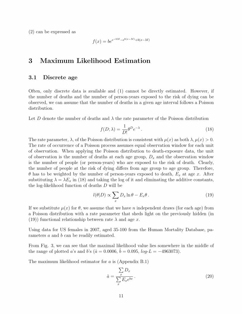
From Fig. 3, we can see that the maximal likelihood value lies somewhere in the middle ofthe range of plotted a’s and b’s (a = 0.0006, b = 0.095, log-L = −4963073).
The maximum likelihood estimator for a is (Appendix B.1)
a =
∑x
Dx∑x
Exebx. (20)
11
−7
−6
−5
−4
−3
−2
−1
Age
log(
µ)
35 40 45 50 55 60 65 70 75 80 85 90 95 100
Figure 2: Observed force of mortality.USA 2007, ages 35-100, females.
ab
logL
Figure 3: Log-likelihood values of a and bfor USA 2007, ages 35-100 data
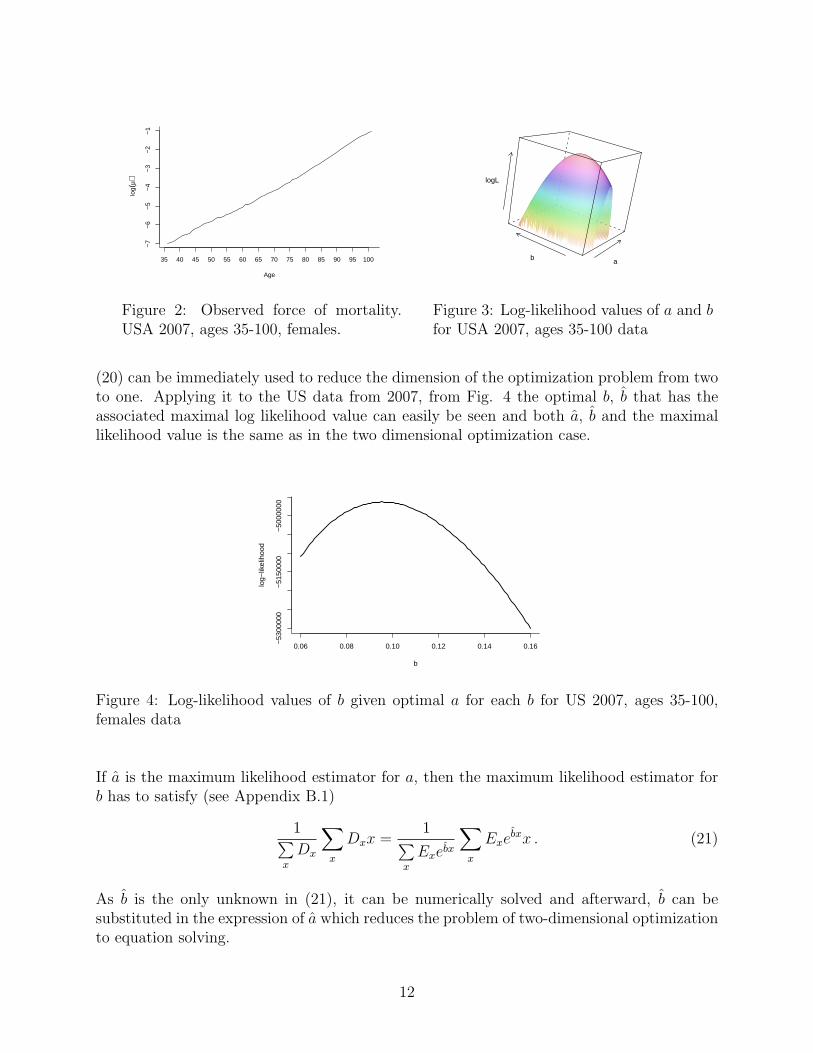
(20) can be immediately used to reduce the dimension of the optimization problem from twoto one. Applying it to the US data from 2007, from Fig. 4 the optimal b, b that has theassociated maximal log likelihood value can easily be seen and both a, b and the maximallikelihood value is the same as in the two dimensional optimization case.
0.06 0.08 0.10 0.12 0.14 0.16
−53
0000
0−
5150
000
−50
0000
0
b
log−
likel
ihoo
d
Figure 4: Log-likelihood values of b given optimal a for each b for US 2007, ages 35-100,females data
If a is the maximum likelihood estimator for a, then the maximum likelihood estimator forb has to satisfy (see Appendix B.1)
1∑x
Dx
∑x
Dxx =1∑
x
Exebx
∑x
Exebxx . (21)
As b is the only unknown in (21), it can be numerically solved and afterward, b can besubstituted in the expression of a which reduces the problem of two-dimensional optimizationto equation solving.
12
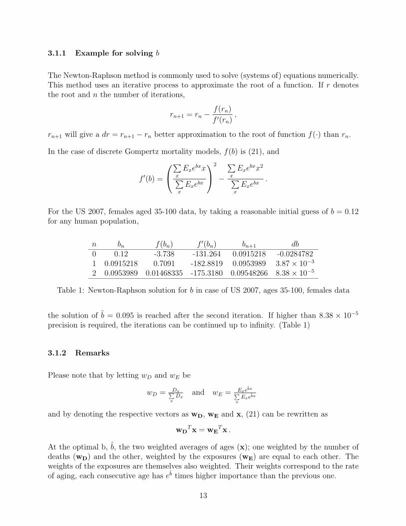
3.1.1 Example for solving b
The Newton-Raphson method is commonly used to solve (systems of) equations numerically.This method uses an iterative process to approximate the root of a function. If r denotesthe root and n the number of iterations,
rn+1 = rn −f(rn)
f ′(rn),
rn+1 will give a dr = rn+1 − rn better approximation to the root of function f(·) than rn.
In the case of discrete Gompertz mortality models, f(b) is (21), and
f ′(b) =
∑x
Exebxx∑
x
Exebx
2
−
∑x
Exebxx2∑
x
Exebx.
For the US 2007, females aged 35-100 data, by taking a reasonable initial guess of b = 0.12for any human population,
n bn f(bn) f ′(bn) bn+1 db0 0.12 -3.738 -131.264 0.0915218 -0.02847821 0.0915218 0.7091 -182.8819 0.0953989 3.87× 10⁻³
2 0.0953989 0.01468335 -175.3180 0.09548266 8.38× 10⁻⁵
Table 1: Newton-Raphson solution for b in case of US 2007, ages 35-100, females data
the solution of b = 0.095 is reached after the second iteration. If higher than 8.38 × 10⁻⁵
precision is required, the iterations can be continued up to infinity. (Table 1)
3.1.2 Remarks
Please note that by letting wD and wE be
wD = Dx∑xDx
and wE = Exebx∑xExebx
and by denoting the respective vectors as wD, wE and x, (21) can be rewritten as
wDTx = wE
Tx .
At the optimal b, b, the two weighted averages of ages (x); one weighted by the number ofdeaths (wD) and the other, weighted by the exposures (wE) are equal to each other. Theweights of the exposures are themselves also weighted. Their weights correspond to the rateof aging, each consecutive age has eb times higher importance than the previous one.
13
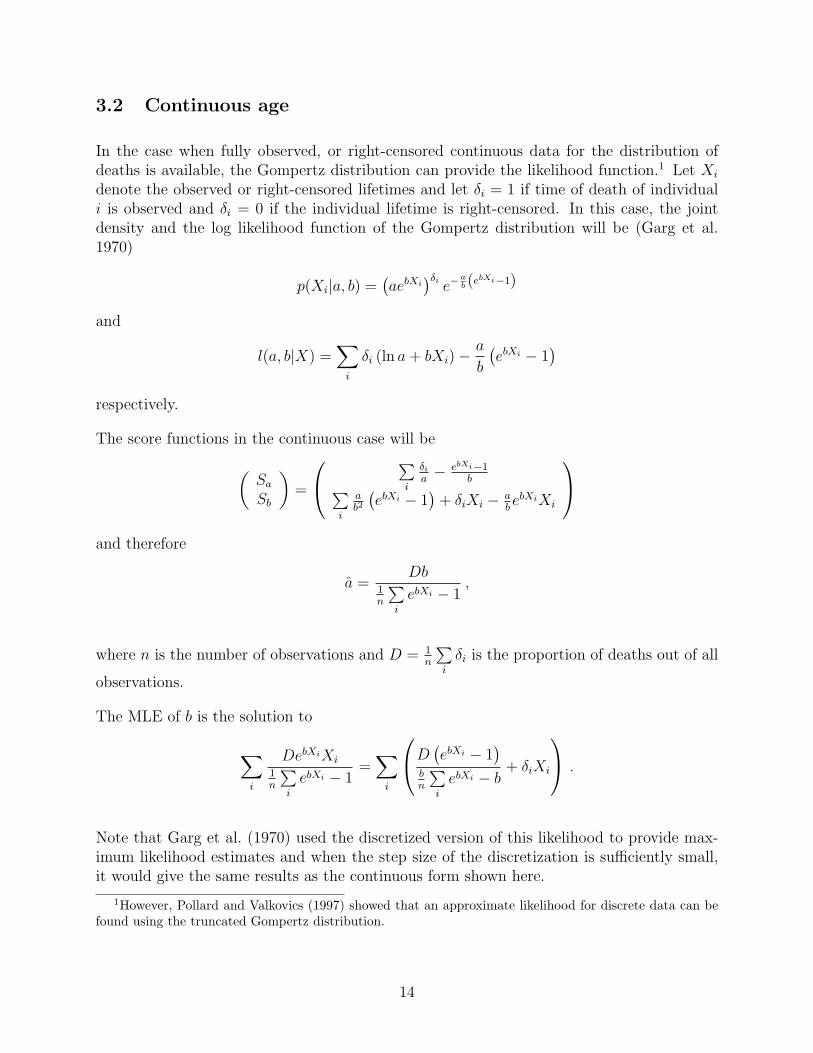
3.2 Continuous age
In the case when fully observed, or right-censored continuous data for the distribution ofdeaths is available, the Gompertz distribution can provide the likelihood function.1 Let Xi
denote the observed or right-censored lifetimes and let δi = 1 if time of death of individuali is observed and δi = 0 if the individual lifetime is right-censored. In this case, the jointdensity and the log likelihood function of the Gompertz distribution will be (Garg et al.1970)
p(Xi|a, b) =(aebXi
)δie−
ab (ebXi−1)
and
l(a, b|X) =∑i
δi (ln a+ bXi)−a
b
(ebXi − 1
)respectively.
The score functions in the continuous case will be(SaSb
)=
∑i
δia− ebXi−1
b∑i
ab2
(ebXi − 1
)+ δiXi − a
bebXiXi
and therefore
a =Db
1n
∑i
ebXi − 1,
where n is the number of observations and D = 1n
∑i
δi is the proportion of deaths out of all
observations.
The MLE of b is the solution to
∑i
DebXiXi
1n
∑i
ebXi − 1=∑i
D (ebXi − 1)
bn
∑i
ebXi − b+ δiXi
.
Note that Garg et al. (1970) used the discretized version of this likelihood to provide max-imum likelihood estimates and when the step size of the discretization is sufficiently small,it would give the same results as the continuous form shown here.
1However, Pollard and Valkovics (1997) showed that an approximate likelihood for discrete data can befound using the truncated Gompertz distribution.
14
3.2.1 Remarks
If all Xi are observed times of death, by denoting the average force of mortality of thepopulation by µ and noting that µ =
∑i
anebXi :
µ = a+ b .
If b = b and the data come from a Gompertz distribution, the observed average force ofmortality is equal to a+ b.
References
Abramowitz, M. and I. Stegun. 1965. Handbook of Mathematical Functions. Washington, DC: USGovernment Printing Office.
Apery, R. 1979. “Irrationalite de ζ (2) et ζ (3).” Asterisque 61:11–13.
Askey, R. A. and A. B. O. Daalhuis. 2010. “Generalized Hypergeometric Functions and Mei-jer G-Function.” In NIST handbook of mathematical functions, edited by F. Olver, D. Lozier,R. Boisvert and C. Clark, Cambridge University Press.
Erdelyi, A. 1953. Higher transcendental functions, vol. 1. New York-Toronto-London: McGraw-Hill.
Garg, M., B. Rao and C. Redmond. 1970. “Maximum-likelihood estimation of the parameters ofthe Gompertz survival function.” Journal of the Royal Statistical Society. Series C (AppliedStatistics) 19(2):152–159.
Gavrilov, L. and N. Gavrilova. 1991. The biology of Life Span: A Quantitative Approach. Chur:Harwood.
Gompertz, B. 1825. “On the Nature of the Function Expressive of the Law of Human Mortality,and on a New Mode of Determining the Value of Life Contingencies.” Philosophical Transactionsof the Royal Society of London 115:513–583.
Gussmann, E. 1967. “Modifizierung der Gewichtsfunktionenmethode zur Berechnung der Fraun-hoferlinien in Sonnen-und Sternspektren.” Zeitschrift fur Astrophysik 65:456–497.
Kunimura, D. 1998. “The Gompertz Distribution-Estimation of Parameters.” Actuarial ResearchClearing House 2:65–76.
Marshall, A. and I. Olkin. 2007. Life Distributions. Springer.
Milgram, M. 1985. “The generalized integro-exponential function.” Mathematics of computation44(170):443–458.
Missov, T. and A. Lenart. 2011. “Linking period and cohort life-expectancy linear increases inGompertz proportional hazards models.” Demographic Research 24(19):455–468.
15
Pollard, J. and E. Valkovics. 1992. “The Gompertz distribution and its applications.” Genus 48(3-4):15–29.
———. 1997. “On the use of the truncated Gompertz distribution and other models to representthe parity progression functions of high fertility populations.” Mathematical Population Studies6(4):291–305.
Preston, S., P. Heuveline and M. Guillot. 2001. Demography: measuring and modeling populationprocesses. Wiley-Blackwell.
Vaupel, J. 1986. “How change in age-specific mortality affects life expectancy.” Population Studies40(1):147–157.
Wetterstrand, W. 1981. “Parametric models for life insurance mortality data: Gompertz’s law overtime.” Transactions of the Society of Actuaries 33:159–175.
Willekens, F. 2002. “Gompertz in context: the Gompertz and related distributions.” In ForecastingMortality in Developed Countries - Insights from a Statistical, Demographic and EpidemiologicalPerspective, European Studies of Population, vol. 9, edited by E. Tabeau, A. van den Berg Jethsand C. Heathcote, pp. 105–126, Springer.
Willemse, W. and H. Koppelaar. 2000. “Knowledge Elicitation of Gompertz’ Law of Morality.”Scandinavian Actuarial Journal pp. 168–180.
A Appendix
A.1 Values of the Ψ function
Note that (Abramowitz and Stegun 1965:6.3.1,6.3.2)
∞∫0
e−u lnu du = ψ(1) = −γ , (22)
where ψ(z) = ddz
ln Γ(z) denotes the digamma function and let ψ(n)(z) = dn
dznψ(z) denote thepolygamma function (Abramowitz and Stegun 1965:6.4.1).
As a special case of ψ(n)(z), when z = 1 (Abramowitz and Stegun 1965:6.4.2),
ψ(n)(1) = (−1)n+1n!ζ(n+ 1) . (23)
16
From (9), (22) and (23),
Ψ0 = limt→0−Γ(1− t) = 1 ;
Ψ1 = limt→0−Γ(1− t)ψ(1− t) = −ψ(1) = γ ;
Ψ2 = limt→0−Γ(1− t) [ψ(1− t)]2 + Γ(1− t)ψ(1)(1− t) = γ2 + ζ(2) ;
...
Ψn = limt→0
dn−1
dtn−1[−Γ(1− t)ψ(1− t)] = lim
t→0
n−1∑k=0
(n− 1
k
)Γ(1− t)(n−1−k)ψ(n−1)(1− t)
(24)
Any values of Ψn can be derived by using relationships (22), (23), ddz
Γ(z) = ψ(z)Γ(z) andΓ(1) = 1.2
A.2 Central moments as Meijer-G functions
Meijer-G functions offer the most succinct way to represent the central moments of theGompertz distribution. The nth order central moment, mn is given as
mn =n∑j=0
(n
j
)(−1)n−jE
[Xj]E [X]n−j
and from (7)
m1 =1
be
abG2,0
1,2
(a
b
∣∣∣∣ ; 10, 0;
)m2 =
2
b2e
abG3,0
2,3
(a
b
∣∣∣∣ ; 1, 10, 0, 0;
)− (m1)
2
m3 =6
b3e
abG4,0
3,4
(a
b
∣∣∣∣ ; 1, 1, 10, 0, 0, 0;
)− 3m1
2
b2e
abG3,0
2,3
(a
b
∣∣∣∣ ; 1, 10, 0, 0;
)+ 2(m1)
3
m4 =24
b4e
abG5,0
4,5
(a
b
∣∣∣∣ ; 1, 1, 1, 10, 0, 0, 0, 0;
)− 4m1
6
b3e
abG4,0
3,4
(a
b
∣∣∣∣ ; 1, 1, 10, 0, 0, 0;
)+ 6(m1)
2 2
b2e
abG3,0
2,3
(a
b
∣∣∣∣ ; 1, 10, 0, 0;
)+ 3(m1)
4 .
2For an alternative derivation (and also for alternative power series expansion of En1 (z)) please see the
Appendix of Gussmann (1967), especially equations (A.39)− (A.41).
17
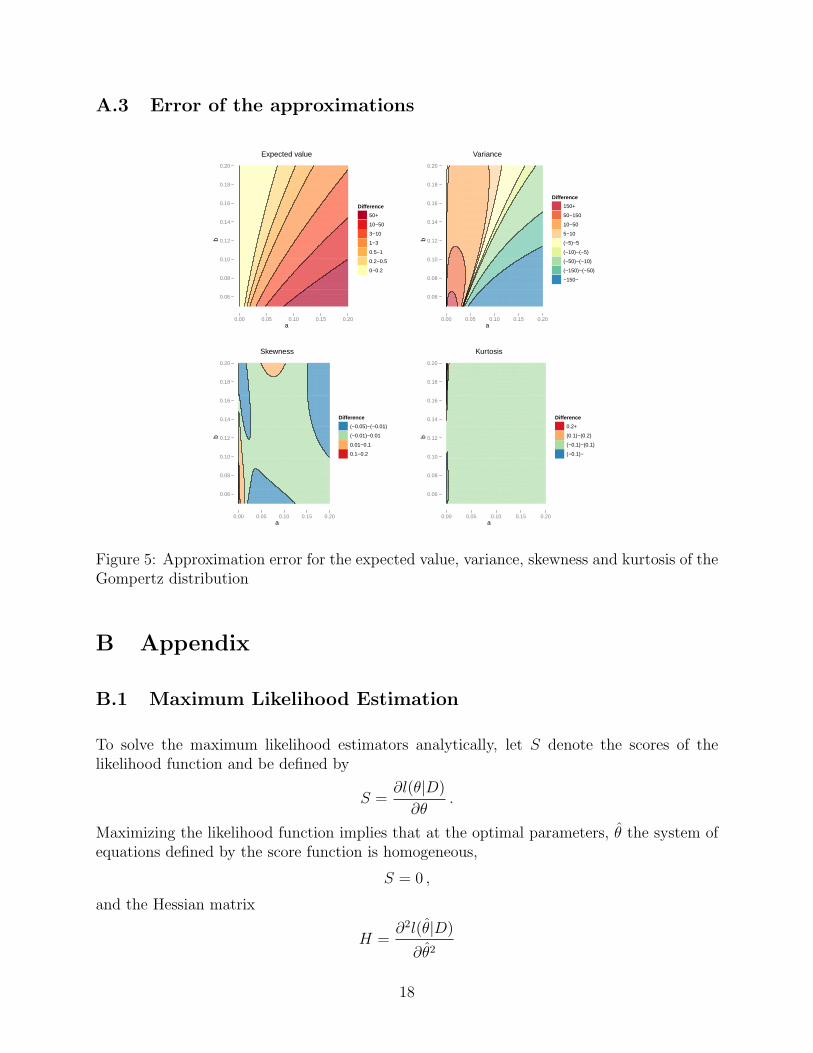
A.3 Error of the approximations
Expected value
a
b
0.06
0.08
0.10
0.12
0.14
0.16
0.18
0.20
0.00 0.05 0.10 0.15 0.20
Difference
50+
10−50
3−10
1−3
0.5−1
0.2−0.5
0−0.2
Variance
a
b
0.06
0.08
0.10
0.12
0.14
0.16
0.18
0.20
0.00 0.05 0.10 0.15 0.20
Difference
150+
50−150
10−50
5−10
(−5)−5
(−10)−(−5)
(−50)−(−10)
(−150)−(−50)
−150−
Skewness
a
b
0.06
0.08
0.10
0.12
0.14
0.16
0.18
0.20
0.00 0.05 0.10 0.15 0.20
Difference
(−0.05)−(−0.01)
(−0.01)−0.01
0.01−0.1
0.1−0.2
Kurtosis
a
b
0.06
0.08
0.10
0.12
0.14
0.16
0.18
0.20
0.00 0.05 0.10 0.15 0.20
Difference
0.2+
(0.1)−(0.2)
(−0.1)−(0.1)
(−0.1)−
Figure 5: Approximation error for the expected value, variance, skewness and kurtosis of theGompertz distribution
B Appendix
B.1 Maximum Likelihood Estimation
To solve the maximum likelihood estimators analytically, let S denote the scores of thelikelihood function and be defined by
S =∂l(θ|D)
∂θ.
Maximizing the likelihood function implies that at the optimal parameters, θ the system ofequations defined by the score function is homogeneous,
S = 0 ,
and the Hessian matrix
H =∂2l(θ|D)
∂θ2
18
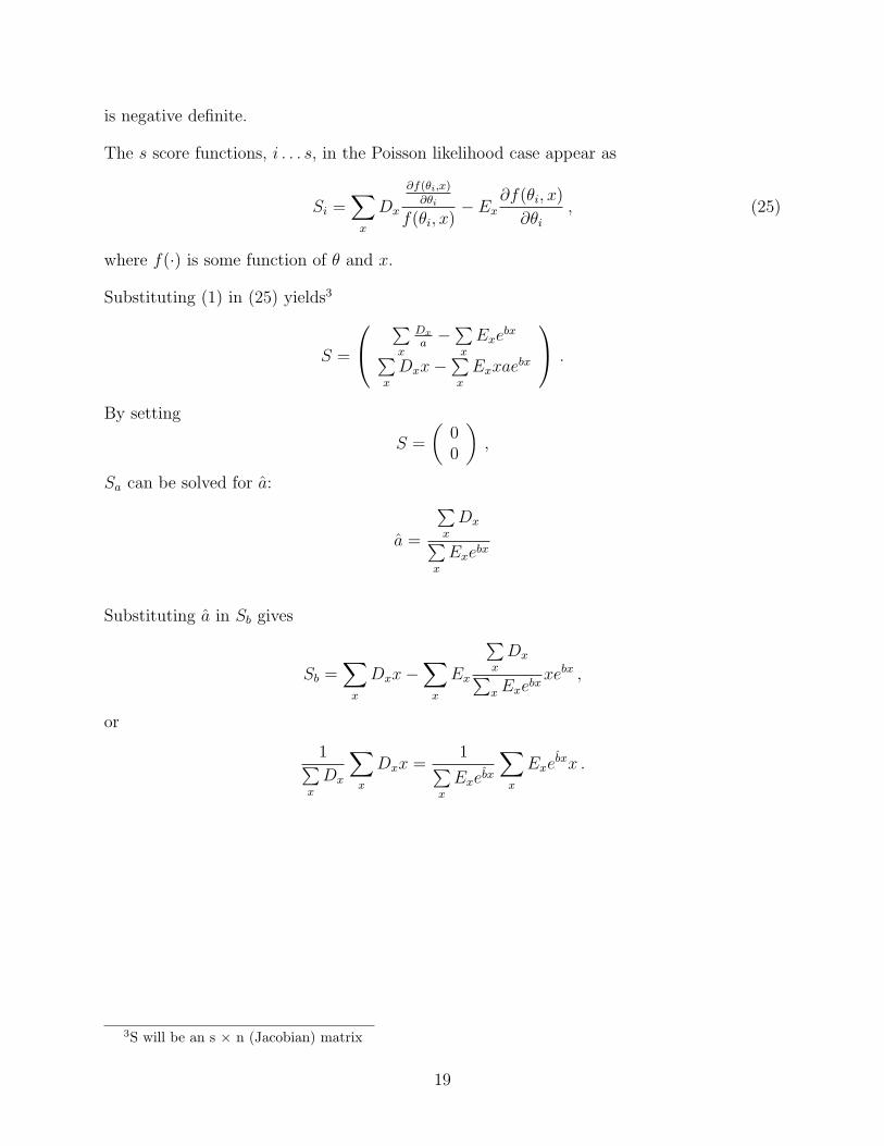
is negative definite.
The s score functions, i . . . s, in the Poisson likelihood case appear as
Si =∑x
Dx
∂f(θi,x)∂θi
f(θi, x)− Ex
∂f(θi, x)
∂θi, (25)
where f(·) is some function of θ and x.
Substituting (1) in (25) yields3
S =
∑x
Dx
a−∑x
Exebx∑
x
Dxx−∑x
Exxaebx
.
By setting
S =
(00
),
Sa can be solved for a:
a =
∑x
Dx∑x
Exebx
Substituting a in Sb gives
Sb =∑x
Dxx−∑x
Ex
∑x
Dx∑xExe
bxxebx ,
or
1∑x
Dx
∑x
Dxx =1∑
x
Exebx
∑x
Exebxx .
3S will be an s × n (Jacobian) matrix
19