The Geography of Development: Evaluating Migration Restrictions and …pubdocs.worldbank.org/en/495511455906842739/The... · The Geography of Development: Evaluating Migration Restrictions

The Geography of Development:Evaluating Migration Restrictions and Coastal Flooding

Klaus DesmetSMU

David Krisztian NagyPrinceton University

Esteban Rossi-HansbergPrinceton University

World Bank, February 2016

Desmet, Nagy and Rossi-Hansberg Geography of Development World Bank, February 2016 1 / 27

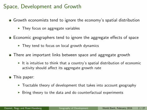
Space, Development and Growth

Growth economists tend to ignore the economy’s spatial distribution

I They focus on aggregate variables

Economic geographers tend to ignore the aggregate effects of space

I They tend to focus on local growth dynamics

There are important links between space and aggregate growth

I It is intuitive to think that a country’s spatial distribution of economicactivity should affect its aggregate growth rate

This paper:

I Tractable theory of development that takes into account geography

I Bring theory to the data and do counterfactual experiments


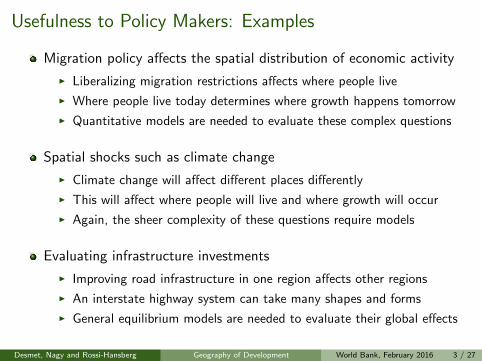
Usefulness to Policy Makers: Examples

Migration policy affects the spatial distribution of economic activity

I Liberalizing migration restrictions affects where people live

I Where people live today determines where growth happens tomorrow

I Quantitative models are needed to evaluate these complex questions

Spatial shocks such as climate change

I Climate change will affect different places differently

I This will affect where people will live and where growth will occur

I Again, the sheer complexity of these questions require models

Evaluating infrastructure investments

I Improving road infrastructure in one region affects other regions

I An interstate highway system can take many shapes and forms

I General equilibrium models are needed to evaluate their global effects


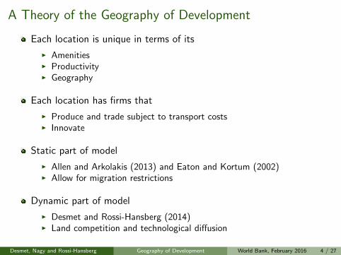
A Theory of the Geography of Development

Each location is unique in terms of its

I AmenitiesI ProductivityI Geography

Each location has firms that

I Produce and trade subject to transport costsI Innovate

Static part of model

I Allen and Arkolakis (2013) and Eaton and Kortum (2002)I Allow for migration restrictions

Dynamic part of model

I Desmet and Rossi-Hansberg (2014)I Land competition and technological diffusion


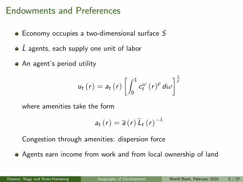
Endowments and Preferences

Economy occupies a two-dimensional surface S

L agents, each supply one unit of labor

An agent’s period utility

ut (r) = at (r)

[∫ 1

0cωt (r)ρ dω

] 1ρ

where amenities take the form

at (r) = a (r) Lt (r)−λ

Congestion through amenities: dispersion force

Agents earn income from work and from local ownership of land


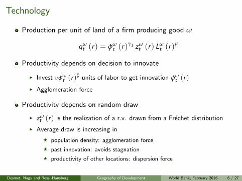
Technology

Production per unit of land of a firm producing good ω

qωt (r) = φω

t (r)γ1 zωt (r) Lω

t (r)µ

Productivity depends on decision to innovate

I Invest νφωt (r)ξ units of labor to get innovation φω

t (r)

I Agglomeration force

Productivity depends on random draw

I zωt (r) is the realization of a r.v. drawn from a Frechet distribution

I Average draw is increasing in

F population density: agglomeration force

F past innovation: avoids stagnation

F productivity of other locations: dispersion force


Productivity Draws and Competition

Productivity draws are i.i.d. across goods, but correlated across space(with perfect correlation as distance goes to zero)

Firms face perfect local competition and innovate

I Firms bid for land up to point of making zero profits after coveringinvestment in technology

Next period all potential entrants have access to same technology

I Dynamic profit maximization simplifies to sequence of static problems

Because of perfect competition, many of the results of EK apply

I The probability that a good produced in r is sold in s is the same asthe share of goods of r sold in s

Firms trade subject to transport costs


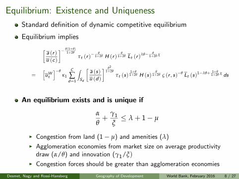
Equilibrium: Existence and Uniqueness

Standard definition of dynamic competitive equilibrium

Equilibrium implies

[a (r )

u (c)

]− θ(1+θ)1+2θ

τt (r )− θ

1+2θ H (r )θ

1+2θ Lt (r )λθ− θ

1+2θ χ

=[uWt

]−θκ1

C

∑d=1

∫Sd

[a (s)

u (d)

] θ2

1+2θ

τt (s)1+θ

1+2θ H (s)θ

1+2θ ς (r , s)−θ Lt (s)1−λθ+ 1+θ

1+2θ χ ds

An equilibrium exists and is unique if

α

θ+

γ1

ξ≤ λ + 1 − µ

I Congestion from land (1 − µ) and amenities (λ)

I Agglomeration economies from market size on average productivitydraw (α/θ) and innovation (γ1/ξ)

I Congestion forces should be greater than agglomeration economies


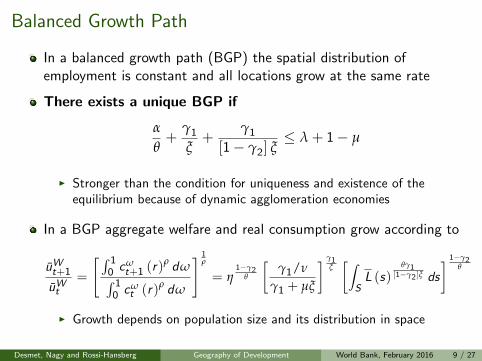
Balanced Growth Path

In a balanced growth path (BGP) the spatial distribution ofemployment is constant and all locations grow at the same rate

There exists a unique BGP if

α

θ+

γ1

ξ+

γ1

[1 − γ2] ξ≤ λ + 1 − µ

I Stronger than the condition for uniqueness and existence of theequilibrium because of dynamic agglomeration economies

In a BGP aggregate welfare and real consumption grow according to

uWt+1

uWt=

[∫ 10 cω

t+1 (r)ρ dω∫ 1

0 cωt (r)ρ dω

] 1ρ

= η1−γ2

θ

[γ1/ν

γ1 + µξ

] γ1ξ[∫

SL (s)

θγ1[1−γ2 ]ξ ds

] 1−γ2θ

I Growth depends on population size and its distribution in space


Calibration: Parameter Values

Use relation between geographic distribution of population andaggregate growth across countries to estimate technology parameters

Use relationship between productivity and amenities in the U.S. toestimate congestion costs

Transport costs use evidence on seas, rivers, lakes, highways, trains,and geographic characteristics

I 64,800 by 64,800 bilateral transport cost matrix

Other parameter values come from the literature


Simulation: Amenities and Productivity

Discretize the world into 1◦ by 1◦ cells (64,800 in total)

Use data on land, population and wages from G-Econ and data onbilateral transport costs to derive spatial distribution of productivityand a (r) /u (c)

Does not separately identify a (r) and u (c)

I Not a problem in models with free mobility (Roback, 1982)

I Not reasonable here: Congo would have very attractive amenities

We need additional data on utility: subjective well-beingMap subjective well-being

I Correlates well with log of income (Kahneman and Deaton, 2010)

I Transform subjective well-being into utility measure that is linear in thelevel of income


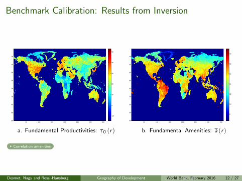
Benchmark Calibration: Results from Inversion

50 100 150 200 250 300 350

20

40

60

80

100

120

140

160

180

-10

0

10

20

30

40

50

50 100 150 200 250 300 350

20

40

60

80

100

120

140

160

180

8

10

12

14

16

18

20

a. Fundamental Productivities: τ0 (r) b. Fundamental Amenities: a (r)

Correlation amenities


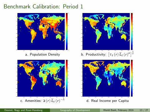
Benchmark Calibration: Period 1

50 100 150 200 250 300 350

20

40

60

80

100

120

140

160

180 -10

-5

0

5

10

15

20

50 100 150 200 250 300 350

20

40

60

80

100

120

140

160

180-2

-1

0

1

2

3

4

5

6

7

8

a. Population Density b. Productivity:[τt (r) Lt (r)

α] 1θ

50 100 150 200 250 300 350

20

40

60

80

100

120

140

160

180 6

7

8

9

10

11

12

13

14

15

16

50 100 150 200 250 300 350

20

40

60

80

100

120

140

160

180

-5

-4

-3

-2

-1

0

1

2

3

c. Amenities: a (r) Lt (r)−λ d. Real Income per Capita


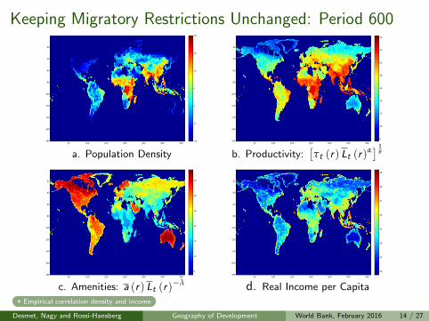
Keeping Migratory Restrictions Unchanged: Period 600

50 100 150 200 250 300 350

20

40

60

80

100

120

140

160

180 -10

-5

0

5

10

15

20

50 100 150 200 250 300 350

20

40

60

80

100

120

140

160

1808

10

12

14

16

18

20

22

24


α] 1θ

50 100 150 200 250 300 350

20

40

60

80

100

120

140

160

1808

10

12

14

16

18

20

50 100 150 200 250 300 350

20

40

60

80

100

120

140

160

18012

13

14

15

16

17

18

19


Empirical correlation density and income


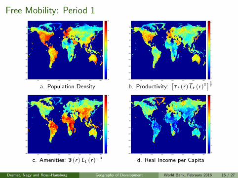
Free Mobility: Period 1

50 100 150 200 250 300 350

20

40

60

80

100

120

140

160

180 -10

-5

0

5

10

15

20

50 100 150 200 250 300 350

20

40

60

80

100

120

140

160

180-2

-1

0

1

2

3

4

5

6

7

8


α] 1θ

50 100 150 200 250 300 350

20

40

60

80

100

120

140

160

180 8

9

10

11

12

13

14

15

16

50 100 150 200 250 300 350

20

40

60

80

100

120

140

160

180-4

-3

-2

-1

0

1

2

3

4



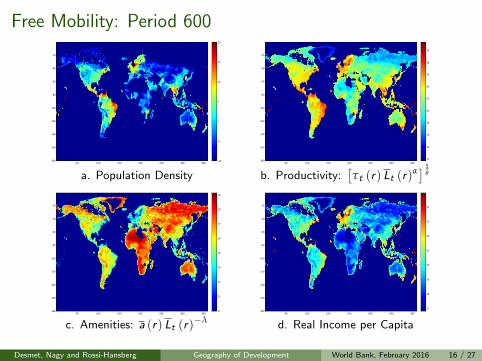
Free Mobility: Period 600

50 100 150 200 250 300 350

20

40

60

80

100

120

140

160

180 -10

-5

0

5

10

15

20

50 100 150 200 250 300 350

20

40

60

80

100

120

140

160

18012

14

16

18

20

22

24

26

28

30


α] 1θ

50 100 150 200 250 300 350

20

40

60

80

100

120

140

160

180 11

12

13

14

15

16

17

18

19

50 100 150 200 250 300 350

20

40

60

80

100

120

140

160

18017

18

19

20

21

22

23

24



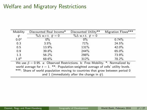
Welfare and Migratory Restrictions

Mobility Discounted Real Income* Discounted Utility** Migration Flows***ψ %∆ w.r.t. ψ = 0 %∆ w.r.t. ψ = 0

0.0a 0% 0% 0.74%0.3 3.5% 71% 24.5%0.5 13.9% 131% 42.0%0.9 39.8% 244% 65.0%1.3 56.2% 298% 73.9%1.8b 68.6% 312% 78.2%We use β = 0.95. a: Observed Restrictions. b: Free Mobility. *: Normalized byworld average for t = 1. **: Population-weighted average of cells’ utility levels.***: Share of world population moving to countries that grow between period 0

and 1 (immediately after the change in ψ).


Rise in Sea Levels

The rise in sea level is a major consequence of global warming

I Thermal expansion of the oceans

I Melting of glaciers and depletion of ice sheetsI Next millennium expected rise by 7 meters

F Likely increase by 0.5 to 1 meter by 2100 (IPCC)

Disproportionate part of the world’s population lives in coastal areas

Existing literature

I Accounting exercises based on current data (Dasgupta et al., 2007)

I Studies contemplating different future scenarios (Nicholls, 2004)

Here: dynamic analysis of rise in sea level by 6 meters


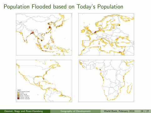
Population Flooded based on Today’s Population

LegendNo Population Flooded0- 50.00050.000 - 500.000500.000 - 1.000.0001.000.000 - 3.000.0003.000.000 - 25.000.000


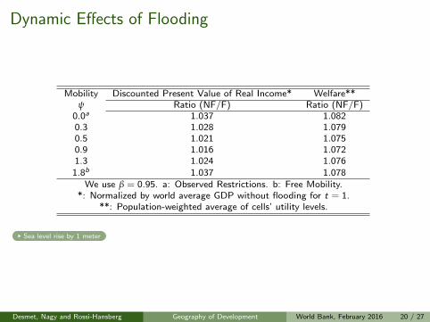
Dynamic Effects of Flooding

Mobility Discounted Present Value of Real Income* Welfare**ψ Ratio (NF/F) Ratio (NF/F)

0.0a 1.037 1.0820.3 1.028 1.0790.5 1.021 1.0750.9 1.016 1.0721.3 1.024 1.0761.8b 1.037 1.078

We use β = 0.95. a: Observed Restrictions. b: Free Mobility.*: Normalized by world average GDP without flooding for t = 1.

**: Population-weighted average of cells’ utility levels.

Sea level rise by 1 meter


Dynamic Effects of Flooding

Flooding reduces real income by 1.6% – 3.7%

It reduces welfare by 7.2% – 8.2%

I Loss in amenities due to flooding are large

In PDV mobility has little effect on the welfare impact of flooding

We would have expected mobility to mitigate negative effects

I Mobility moves more people to coastal areas

I People move to places that are individually, not socially, beneficial

I Local migration argument no longer works with complex geography


Conclusion

Interaction between geography and economic development throughtrade, technology diffusion and migration

Connect to real geography of the world at fine detail

Relaxing migration restrictions can lead to very large welfare gains

Level of migration restrictions will have important effect on whichregions of the world will be the productivity leaders of the future

Coastal flooding will have important welfare effects

I Mobility has little effect on the welfare effect of flooding


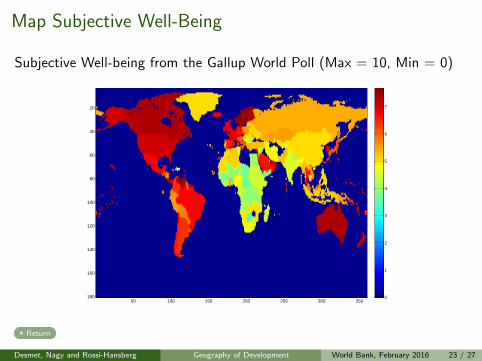
Map Subjective Well-Being

Subjective Well-being from the Gallup World Poll (Max = 10, Min = 0)

50 100 150 200 250 300 350

20

40

60

80

100

120

140

160

180 0

1

2

3

4

5

6

7

Return


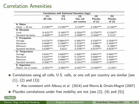
Correlation AmenitiesCorrelations with Estimated Amenities (logs)

(1) (2) (3) (4) (5)All cells U.S. One cell Placebo Placebo

per country of (1) of (3)A. WaterWater < 50 km 0.2198*** 0.1286*** 0.1232** 0.1064*** -0.1363**B. ElevationLevel -0.4152*** -0.1493*** -0.2816*** -0.2793*** 0.1283**Standard deviation -0.4599*** -0.2573*** -0.3099*** -0.3285*** 0.1121*C. PrecipationAverage 0.4176*** 0.08643*** 0.3851*** 0.3185*** 0.1830***Maximum 0.4408*** 0.1068*** 0.3128*** 0.4286*** 0.3200***Minimum 0.2035*** 0.2136*** 0.2108*** -0.0096 -0.1965**Standard deviation 0.4160*** 0.0212 0.2746*** 0.4715*** 0.4535***D. TemperatureAverage 0.6241*** 0.6928*** 0.3087*** 0.6914*** 0.5692***Maximum 0.5447*** 0.7388*** 0.1276*** 0.6589*** 0.4635***Minimum 0.6128*** 0.6060*** 0.2931*** 0.6565*** 0.5389***Standard deviation -0.5587*** -0.3112*** -0.3313*** -0.5539*** -0.3679***E. VegetationDesert, ice or tundra -0.3201*** -0.3993*** -0.1827*** -0.2440*** -0.1291*

Correlations using all cells, U.S. cells, or one cell per country are similar (see

(1), (2) and (3))

I Also consistent with Albouy et al. (2014) and Morris & Ortalo-Magne (2007)

Placebo correlations under free mobility are not (see (2), (4) and (5))

Return


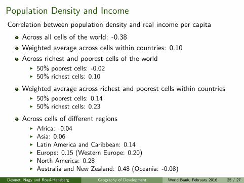
Population Density and Income

Correlation between population density and real income per capita

Across all cells of the world: -0.38

Weighted average across cells within countries: 0.10

Across richest and poorest cells of the worldI 50% poorest cells: -0.02I 50% richest cells: 0.10

Weighted average across richest and poorest cells within countriesI 50% poorest cells: 0.14I 50% richest cells: 0.23

Across cells of different regionsI Africa: -0.04I Asia: 0.06I Latin America and Caribbean: 0.14I Europe: 0.15 (Western Europe: 0.20)I North America: 0.28I Australia and New Zealand: 0.48 (Oceania: -0.08)


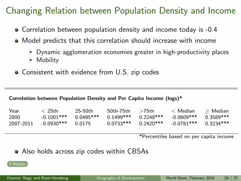
Changing Relation between Population Density and Income

Correlation between population density and income today is -0.4

Model predicts that this correlation should increase with income

I Dynamic agglomeration economies greater in high-productivity placesI Mobility

Consistent with evidence from U.S. zip codes

Correlation between Population Density and Per Capita Income (logs)*

Year < 25th 25-50th 50th-75th >75th < Median ≥ Median2000 -0.1001*** 0.0495*** 0.1499*** 0.2248*** -0.0609*** 0.3589***2007-2011 -0.0930*** 0.0175 0.0733*** 0.2420*** -0.0781*** 0.3234***

*Percentiles based on per capita income

Also holds across zip codes within CBSAs

Return


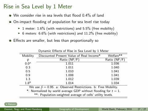
Rise in Sea Level by 1 Meter

We consider rise in sea levels that flood 0.4% of land

On-impact flooding of population for sea level rise today

I 1 meter: 1.6% (with restrictions) and 5.5% (free mobility)I 6 meters: 6.6% (with restrictions) and 11.2% (free mobility)

Effects are smaller, but less than proportionally so

Dynamic Effects of Rise in Sea Level by 1 Meter

Mobility Discounted Present Value of Real Income* Welfare**ψ Ratio (NF/F) Ratio (NF/F)

0.0a 1.011 1.0360.3 1.011 1.0400.5 1.010 1.0410.9 1.008 1.0411.3 1.012 1.0391.8b 1.014 1.034

We use β = 0.95. a: Observed Restrictions. b: Free Mobility.*: Normalized by world average GDP without flooding for t = 1.

**: Population-weighted average of cells’ utility levels.

Return


Documents

The Geography of Development: Evaluating Migration Restrictions and …pubdocs.worldbank.org/en/495511455906842739/The... · The Geography of Development: Evaluating Migration Restrictions