The geography of agriculture participation and food

RESEARCH Open Access

The geography of agriculture participationand food security in a small and a medium-sized city in GhanaHayford Mensah Ayerakwa1*, Fred Mawunyo Dzanku2 and Daniel Bruce Sarpong3

* Correspondence: [email protected]; [email protected] of Ghana LearningCentres, School of Continuing andDistance Education, University ofGhana, Accra, GhanaFull list of author information isavailable at the end of the article

Abstract

The debate about the contribution of urban agriculture to urban household foodsecurity has not considered the possible differential effects by geography ofproduction activities, focusing either on urban household’s participation inagriculture irrespective of where the activity takes place, or restricting participation toproduction within urban and peri-urban areas, or more narrowly, production withinbuild-up urban spaces. Using a sample of 2004 households in a small and amedium-sized city in Ghana, this article contributes by disentangling urbanhousehold’s participation in agriculture by geography of production activities andthe implications for the food security of urban households. We find no evidencefrom our sample that participation in agriculture in general matters for the foodsecurity of urban households. However, urbanites who produced food in both urbanand rural areas had better food security in the medium-sized city.

Keywords: Urban agriculture, Food production, Food security, Techiman, Tamale,Ghana

IntroductionSeveral benefits of urban agriculture (UA) have been mentioned in the literature,

including ecosystem services provisioning, social values, and health benefits (Clin-

ton et al. 2018; Weidner et al. 2019). In this article, however, we focus on the

contribution of UA to urban household food security (FS). UA has received con-

siderable attention over the last decade for its actual and potential contribution to

reducing food insecurity and poverty among urban households (Gerstl et al. 2002;

Rogerson 2003; Mougeot 2005; Shifa and Borel-Saladin 2019). UA has been pro-

moted by some civil society organizations, researchers, government agencies, and

development agencies as a pro-poor initiative in developing countries (Mougeot

2006; Lee-Smith 2010; Clinton et al. 2018). Proponents argue that UA is an im-

portant source of food in most developing countries and is a critical food and nu-

trition security strategy among the urban poor (Armar-Klemesu 2000; Mougeot

2000; Nugent 2000; Maxwell 2001).

© The Author(s). 2020 Open Access This article is licensed under a Creative Commons Attribution 4.0 International License, whichpermits use, sharing, adaptation, distribution and reproduction in any medium or format, as long as you give appropriate credit to theoriginal author(s) and the source, provide a link to the Creative Commons licence, and indicate if changes were made. The images orother third party material in this article are included in the article's Creative Commons licence, unless indicated otherwise in a creditline to the material. If material is not included in the article's Creative Commons licence and your intended use is not permitted bystatutory regulation or exceeds the permitted use, you will need to obtain permission directly from the copyright holder. To view acopy of this licence, visit http://creativecommons.org/licenses/by/4.0/.

Agricultural and FoodEconomics

Ayerakwa et al. Agricultural and Food Economics (2020) 8:10 https://doi.org/10.1186/s40100-020-00155-3

http://crossmark.crossref.org/dialog/?doi=10.1186/s40100-020-00155-3&domain=pdf

mailto:[email protected]



http://creativecommons.org/licenses/by/4.0/

The above notwithstanding, there is a continuing debate about the actual con-

tribution of UA to urban food supply as a whole and to the food and nutrition

security of participating urbanites in particular. Many authors (Ellis and Sum-

berg 1998; Zezza and Tasciotti 2010; Crush et al. 2011; Lee-Smith 2013; Stewart

et al. 2013; Frayne et al. 2014) argue that the importance of UA for urban

household FS has been overstated. For example, using nationally representative

data for 15 countries including four from Africa, Zezza and Tasciotti (2010)

found a positive association between participation in UA and FS in two of the

African countries (Ghana and Nigeria) included in their sample. However, they

cautioned that the positive relationship should not be overstated because of the

minimal contribution of UA to the income of participating households; Ellis and

Sumberg (1998) provided similar caution. Based on results of their study of 19

countries (including six from Africa), Badami and Ramankutty (2015) are even

more doubtful about the contribution of UA to FS. They conclude as follows:

“UA can only make a limited contribution to urban FS, let alone FS generally, in

low-income countries” (p. 14).

As could be expected how UA is defined and measured matters for the con-

clusions one might reach, both with respect to the magnitude of participation

and the association between UA and FS (Warren et al. 2015). The three most

common definitions of UA in the literature are (a) crop and livestock production

by urbanites irrespective of where the activity takes place (e.g., Zezza and Tas-

ciotti 2010), (b) crop and livestock production within urban and peri-urban

spaces irrespective of who is involved (e.g., Lee-Smith 2010), and (c) the growing

of crops in cities (e.g., Clinton et al. 2018). Some authors (e.g., Badami and

Ramankutty 2015) define UA more narrowly as primary vegetable production in

“built-up” urban areas. Clearly, the association between UA and FS would de-

pend on which of these definitions is applied. As an empirical point of departure

from the received literature, the present article applies the first definition of UA

mutatis mutandis as explained below.

Policies and institutions play a role in either promoting or inhibiting UA and

its poverty and food insecurity reducing potential (Bryld 2003; Smit 2016). In

Ghana for example, one of the six components of the Medium Term Agriculture

Development Plan for the period 2011–2015 (METASIP I) was termed “Support

to Urban and Peri-Urban Agriculture” (MoFA 2010). The program acknowledged

urban and peri-urban agriculture as major contributors to national FS. Thus, the

government of Ghana, unlike their counterparts in most African countries,

viewed UA as important for FS and therefore sorts to promote it through an

agricultural policy. However, it must be noted that the policy did not consider

the interplay between agricultural production by urbanites in urban and rural

spaces and urban household FS. In this sense, the policy did not contextualize

UA in small and medium-sized cities (Ayerakwa 2017). It is worth noting that

when the METASIP was revised in 2014, leading to the formulation of the

METASIP II for the period 2014–2017, UA was mentioned only once in the en-

tire policy document and was in relation to food safety, not an advocacy for

promoting UA. This probably reflects a change in policy emphasis as pressure

on urban lands continues to rise.

Ayerakwa et al. Agricultural and Food Economics (2020) 8:10 Page 2 of 21

It can be argued that the main concern of policy makers, practitioners, and

urbanites within the context of increasing urbanization and rising urban pov-

erty in Africa should be how UA as a livelihood activity contributes to poverty

and food insecurity reduction rather than where the activity takes place per

se. At the same time, however, the availability of land—the most important re-

source required for UA in Africa—could depend on proximity to peri-urban

and rural areas. Yet, as observed by Abu Hatab et al. (2019b), the available

UA literature has neglected interactions between urban and rural areas in

urban food systems. For example, the UA literature has not considered the

differential FS outcomes of food production by urbanites beyond urban and

peri-urban boundaries.

Another important research issue that remains unaddressed, which is directly

related to the gap identified in the UA literature by Abu Hatab et al. (2019b),

is whether the opportunity for agricultural production by urbanites in both

urban and rural areas matter for the FS of urban households. Living in an

urban area and yet producing food in rural areas could be an important way of

overcoming the land constraint to agricultural production within built-up urban

areas.

Another gap in the literature relates to the paucity of knowledge on UA and

FS in rapidly urbanizing secondary cities, which is partly due to the overcon-

centration of UA research on primary cities—Accra and Kumasi in the case of

Ghana—although secondary cities tend to face the most pressing challenges

and vulnerabilities to poverty and food insecurity (Battersby and Watson

2019). Zezza and Tasciotti (2010) also called for detailed and rigorous

country-specific case studies to aid understanding of the precise magnitude

and effects of UA.

Based on the gaps in the literature outlined above, the main objective of this

article is to examine urban households’ participation in agricultural production

in both urban and rural areas and the implications for urban household FS. Ad-

dressing this objective contributes to the UA and FS literature in two major

ways: first, by examining the household FS implications of food production by

urbanites in both urban and rural areas rather than focusing on production in

either urban or peri-urban spaces and second, we contribute by breaking away

from the “large city” bias to provide evidence from the perspective of a small

and a medium-sized city.

By employing statistically representative samples of households in two of

Ghana’s fastest growing urban areas—rather than a sample of UA participants

as most studies have done (Poulsen et al. 2015)—we provide further and bet-

ter understanding of the association between the geography of urban house-

holds’ food provisioning arrangements and their FS. This approach is more

relevant for unraveling important policy implications for UA, FS, and urban

planning in general. The relevance of our approach could also be viewed

within the context of increasing urbanization, which is associated with rising

urban land values and thus makes the opportunity cost of putting such lands

under agriculture prohibitively high. Such opportunity cost could be moder-

ated by proximity to rural areas where pressure on land is lower, which is


why it is important to differentiate between the FS effects of urban house-

holds’ engagement in agriculture in urban areas on the one hand and rural

areas on the other.

The rest of the paper is structured as follows. The next section describes the method-

ology by first providing a contextual background that informed the sampling strategy

within the cities. The “Methodology” section also provides and analytical framework,

describes the key variables employed, and presents the empirical econometric models.

The results from the analyses are presented and discussed in the fourth section; the

final section concludes.

MethodologyThe cities and sampling

The data for this study comes from the Ghana component of the African Urban Agri-

culture Project. Techiman (in the Bono East regional capital) and Tamale (in the

Northern regional capital)1 were purposively selected to break away from the large city

bias that has characterized UA research in Ghana and other African countries. Table 1

presents selected characteristics of the two cities based on the most current census data

that was collected in 2010 (Ghana Statistical Service 2014b; 2014a). We classified the

cities as small and medium based on their relative population sizes. Whereas Techiman

is classified as a municipal assembly, Tamale is classified as a metropolitan assembly.

According to the 2010 census, the population of the Techiman Municipality was 147,

788, but only about 64% lived in urban localities. Thus, the population of Techiman

“city” was about 95,323. On the other hand, about 81% of the 233,252 inhabitants of

the Tamale Metropolis lived in urban localities, meaning that the population of Tamale

“city” was about 188,468. The population density is higher in Tamale than Techiman

(Table 1).

To address the objective of this article, we carried out a survey that aimed at

a representative random sample of households in each city. Based on the esti-

mates in Table 1, the population of households at the time of the survey was

25,404 and 31,257 for Techiman and Tamale, respectively. According to Yamane

(1967), the minimum sample size based on a random draw in this case can be

determined by:

n ¼ N1þN e2ð Þ ;

where n is the sample size, N is the population of interest (i.e., number of households),

and e is the margin of error. With 5% margin of error (i.e., e = 0.05), we needed a mini-

mum of 400 households in each city. However, in order to increase the reliability of

our results with higher precision and given that the sample frame was old (based on

the 2010 population census), we randomly sampled 1000 households from each city. In

addition to increasing the reliability and precision of our estimates, a larger sample pro-

vides adequate data that allows for the kind of rigorous statistical analysis that is

1At the time of the survey in 2013, Ghana was divided into 10 administrative regions. Techiman was locatedin the Brong-Ahafo Region while Tamale was in the Northern Region. In 2019, some of the 10 regions weresub-divided. The Bono East Region was carved out of the Brong-Ahafo Region, with Techiman as the new re-gional capital—a testament to its rapid growth.2https://www.afsun.org/


https://www.afsun.org/

lacking in most of the UA literature as pointed out in a recent systematic review by

Abu Hatab et al. (2019b).

The survey questionnaire was based on that developed by African Food Secur-

ity Urban Network (AFSUN).2 The questionnaire captured information on

household structure, housing characteristics, household cash income from all

sources, household food access, dietary diversity, months of adequate food pro-

visioning, food price changes, food sources, agricultural activities, food transfers,

and food aid. The household survey data was complemented by qualitative in-

terviews in August 2015 with opinion leaders in the two cities. In all, we con-

ducted 11 and 10 key informant interviews in Techiman and Tamale,

respectively. The reason for the qualitative interviews was to provide additional

insights into institutional arrangements governing ownership and use of land in

the two cities, and implications for urban food security, if any. It also provided

the opportunity to seek contextual explanations for key findings from the sur-

vey. The qualitative interviews focused on motivations for engagement in agri-

culture, access to land for UA, and the general land holding arrangements in

the cities.

Analytical framework and key indicators

Food security (FS) is a multidimensional phenomenon, which has four arms or pillars,

namely food availability, access, utilization, and stability (FAO 2009). This article essen-

tially focuses on the availability and access dimensions of FS. At the household level, FS

can be achieved through at least three pathways: own production, food markets, and

food transfers (Dzanku 2019). Conceptually, we can represent FS as a function of these

pathways as:

FS ¼ f own production;market; food transferð Þ: ð1Þ

This means that own food production may not be necessary for the attainment of FS

among urban households in particular. Urbanites could allocate household resources

towards activities that yield the highest return, subject to factor market constrains, and

then use the income gained from such activities to purchase food thus achieving FS via

the food market arm. Analytically therefore, the question of whether or not urbanites

who are engaged in food production have better FS than those who do not engage in

the activity is undetermined, and the answer must be found in specific empirical

contexts.

Table 1 Selected characteristics of the two cities

Indicators Urban Techiman Urban Tamale

2010 census population 95,323 188,468

Estimated annual population growth rate (%) 2.6 2.2

Population density (persons per km2) 227.7 360.6

Number of households 23,566 29,322

Mean household size 4.0 6.3

Percent of households engaged in agriculture 33.0 26.1

Source: Ghana Statistical Service (2014a and 2014b)


The outcome variable of interest in this article is a measure of household FS.

Following Coates et al. (2007), we use the Household Food Insecurity Access

Scale (HFIAS) to classify households as food secure or not based on a set of

nine questions. The questions take into account a reflection on several food in-

security experiences including hunger, anxiety about household food access and

preferences, and worrying about food adequacy (Headey and Ecker, 2013). The

information generated by the HFIAS is used to assess the prevalence of house-

hold food insecurity (Coates et al. 2007).

Respondents were asked each of the HFIAS questions with a recall period of 4

weeks. This allowed them to assess, first, the occurrence of food insecurity, and

then the frequency of different types of food insecurity occurrences. This allows

a determination of whether food insecurity occurred rarely (once or twice),

sometimes (three to ten times), or often (more than ten times) over a 4-week

period (Coates et al. 2007; Headey and Ecker 2013).

Following Coates et al. (2007), we use HFIAS to classify households into four categor-

ies of household food insecurity access prevalence (HFIAP) status: (a) food secure, (b)

mildly food insecure, (c) moderately food insecure, and (d) severely food insecure. In

this article, we recast all the food insecurity indicators in the “positive scale” so that we

can refer to them as FS indicators rather than food insecurity measures. Thus, we let

FSi denote the category—severely food insecure (FS = 0), moderately food insecure (FS

= 1), mildly food insecure (FS = 2), and food secure (FS = 3)—to which household i be-

longs. These four categories present a measure of logically ordered household FS status

of households in the two cities. We also define a binary food security indicator, FSD,

simply as

FSD ¼ 1 if FS ¼ 30 otherwise

�ð2Þ

Lastly, rather than use the above categorical variables constructed from the HFIAS,

which could lead to information loss, we simply use the HFIAS score, which ranges be-

tween 0 and 27. As before, we recast the food insecurity score into FS score, which we

refer to as Household Food Security Access Scale Score (HFSASS) by simply subtract-

ing the HFIAS score from 27 so that the larger the value of the score the more food se-

cure a household is.

The validity of the HFIAS indicator has been tested comprehensively and

found to have several advantages including the ability of the scale to capture

psychological dimensions of food insecurity. It has been widely acknowledged as

a valid and internally consistent tool for measuring the access component of FS

(Becquey et al. 2010; Salarkia et al. 2014; Gebreyesus et al. 2015). Nonetheless,

Headey and Ecker (2013) argue that the indicator lacks comparability across

wealth and education groups in some contexts and has the tendency to under-

estimate food insecurity due to feelings of shame associated with admission of

hunger.

Our main research question is whether the association between UA and FS de-

pends on where agricultural production takes place—that is, whether in urban

spaces (including peri-urban spaces) only, rural spaces only, or both. Thus, the

main explanatory variable of interest is the location of crop and livestock


production by urban households. Let prodloc denotes the category—nonpartici-

pation in agriculture (prodloc = 1), production in urban space only (prodloc =

2), production in rural space only (prodloc = 3), and production in both urban

and rural spaces (prodloc = 3)—to which urban household i belongs. Differences

in FS between the four groups of households are undetermined a priori because,

as our conceptual model in equation (1) shows, urban households could achieve

FS without food self-provisioning.

Empirical econometric model

We first model the association between FS and urban household participation in

agriculture using the FS score (HFSASS) as the dependent variable. We use the

Tobit estimator because nearly 47% of households did not experience food inse-

curity and therefore have the maximum score of 27. The model can be written

as:

hfsass�i ¼ αþ δ1Nonpi þ δ2Uonlyi þ δ3Ronlyþ β0Xi þ εi;where εi∼Normal 0; σ2ε

� �hfsass ¼ max hfsass�i ; 27

� �ð3Þ

where Nonp, Uonly, and Ronly are the urban agriculture participation categories,

meaning that UandR is the base category;. Xi is the vector of control variables; and εi is

the random error term.

Second, we use the probit estimator when the dependent variable is the binary FS

indicator:

FSD�i ¼ αþ γ1Nonpi þ γ2Uonlyi þ γ3Ronlyþ β

0Xi þ εi; ð4Þ

where FSD�i is the latent unobserved level of FS for household i, which is related to

the binary outcome FSDi by

FSDi ¼ 1 if FSD�i > 0

0 otherwise

�

Finally, since the household food security access prevalence (hfsap) status indicator is

ordinal, we specify an ordered probit model. The probability of observing a given hfsap

status is estimated as:

hfsap�i ¼ αþ φ1Nonpi þ φ2Uonlyi þ φ3Ronlyþ β0Xi þ εi; hfsapi ¼ j if μ j−1

< hfsap�i < μi ð5Þ

where μ is the threshold parameter (or the number of possible outcomes, which in this

case is four); ε is assumed to be normally distributed; and all other variables and pa-

rameters are as defined earlier.

Our choice of control variables in the vector X of Eqs. (3)–(5) was informed

by the conceptual model in Eq. (1), which is based on the food security litera-

ture (e.g., Burchi and De Muro 2016; Frelat et al. 2016). These include house-

hold demographic characteristics, human capital indicators, income, nonfarm

employment, stock of wealth in the form of livestock and other assets, and so-

cial network capital that could manifest in the form of private cash and kind

transfers. An idiosyncratic shock could render an otherwise food secure


household insecure. Therefore, we include indicators such as chronic illness,

unemployment, and indebtedness as control variables. Finally, the full sample

regressions contain a city dummy as an explanatory variable to capture city-

specific effects.

Results and discussionDescriptive analysis

Our survey data shows that about 44% of households in the two cities produced

crops and/or raised livestock, whether in urban or rural spaces or both—some

estimates in the literature (Zezza and Tasciotti 2010) reported participation rates

between 11% and 69%. Participation in agriculture does not differ significantly

across the two cities—about 44% in Techiman and 43% in Tamale (p value =

0.506). For those involved in agriculture, production in only urban spaces

(Uonly) was more common than production in rural spaces only (Ronly)—about

48% versus 41%. Only about 12% of those engaged in agriculture produced in

both urban and rural areas (UandR).

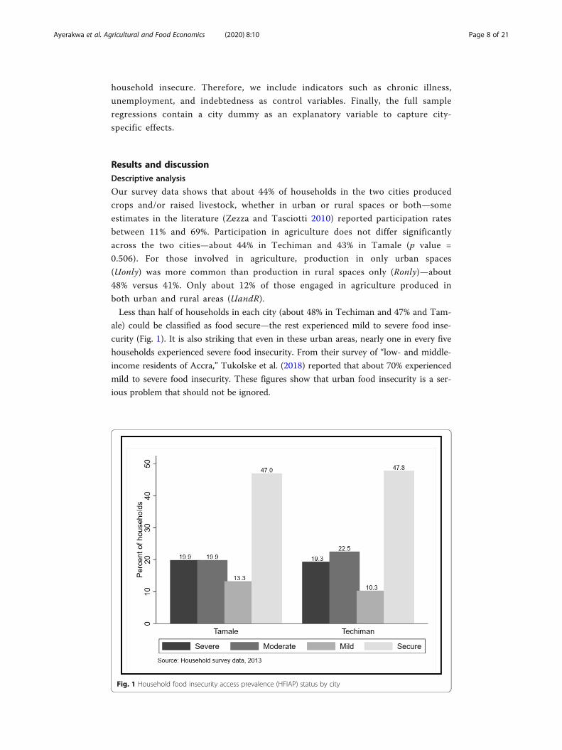
Less than half of households in each city (about 48% in Techiman and 47% and Tam-

ale) could be classified as food secure—the rest experienced mild to severe food inse-

curity (Fig. 1). It is also striking that even in these urban areas, nearly one in every five

households experienced severe food insecurity. From their survey of “low- and middle-

income residents of Accra,” Tukolske et al. (2018) reported that about 70% experienced

mild to severe food insecurity. These figures show that urban food insecurity is a ser-

ious problem that should not be ignored.

Fig. 1 Household food insecurity access prevalence (HFIAP) status by city


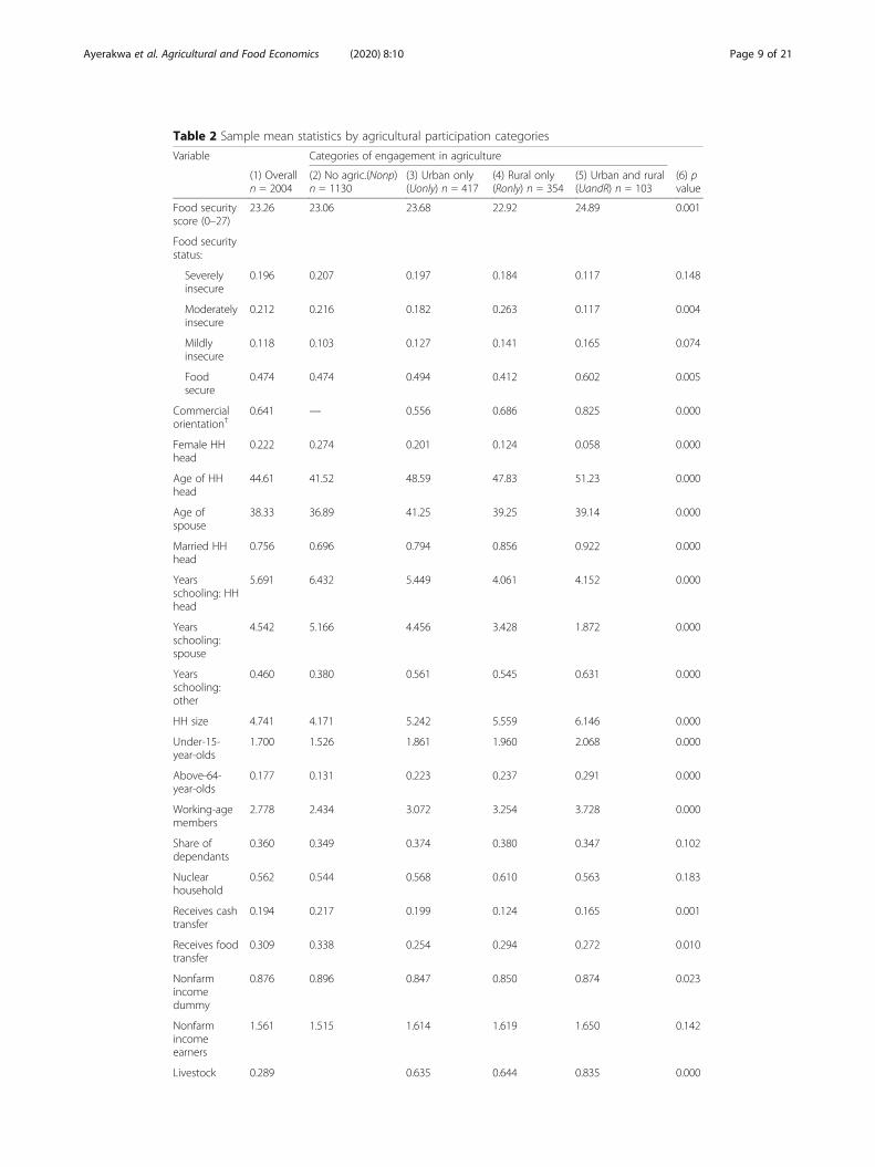
Table 2 Sample mean statistics by agricultural participation categories

Variable Categories of engagement in agriculture

(1) Overalln = 2004

(2) No agric.(Nonp)n = 1130

(3) Urban only(Uonly) n = 417

(4) Rural only(Ronly) n = 354

(5) Urban and rural(UandR) n = 103

(6) pvalue

Food securityscore (0–27)

23.26 23.06 23.68 22.92 24.89 0.001

Food securitystatus:

Severelyinsecure

0.196 0.207 0.197 0.184 0.117 0.148

Moderatelyinsecure

0.212 0.216 0.182 0.263 0.117 0.004

Mildlyinsecure

0.118 0.103 0.127 0.141 0.165 0.074

Foodsecure

0.474 0.474 0.494 0.412 0.602 0.005

Commercialorientation†

0.641 — 0.556 0.686 0.825 0.000

Female HHhead

0.222 0.274 0.201 0.124 0.058 0.000

Age of HHhead

44.61 41.52 48.59 47.83 51.23 0.000

Age ofspouse

38.33 36.89 41.25 39.25 39.14 0.000

Married HHhead

0.756 0.696 0.794 0.856 0.922 0.000

Yearsschooling: HHhead

5.691 6.432 5.449 4.061 4.152 0.000

Yearsschooling:spouse

4.542 5.166 4.456 3.428 1.872 0.000

Yearsschooling:other

0.460 0.380 0.561 0.545 0.631 0.000

HH size 4.741 4.171 5.242 5.559 6.146 0.000

Under-15-year-olds

1.700 1.526 1.861 1.960 2.068 0.000

Above-64-year-olds

0.177 0.131 0.223 0.237 0.291 0.000

Working-agemembers

2.778 2.434 3.072 3.254 3.728 0.000

Share ofdependants

0.360 0.349 0.374 0.380 0.347 0.102

Nuclearhousehold

0.562 0.544 0.568 0.610 0.563 0.183

Receives cashtransfer

0.194 0.217 0.199 0.124 0.165 0.001

Receives foodtransfer

0.309 0.338 0.254 0.294 0.272 0.010

Nonfarmincomedummy

0.876 0.896 0.847 0.850 0.874 0.023

Nonfarmincomeearners

1.561 1.515 1.614 1.619 1.650 0.142

Livestock 0.289 0.635 0.644 0.835 0.000


Table 2 presents mean summary statistics of variables employed in the regression

analyses by the four agriculture engagement categories (i.e., Nonp, Uonly, Ronly, and

UandR). The average household food security access scale score is about 23 out of a

maximum score of 27; the scores are not statistically identical across the four groups of

urban households, as the p value in column (6) shows. Urban households who pro-

duced food in both urban and rural areas have a higher mean FS score than the other

groups. The Household Food Insecurity Access Prevalence (HFIAP) status indicator

shows that severe food insecurity is least common among UandR households. Similarly,

a higher proportion (60%) UandR households were food secure compared with only

47% in the overall sample.

The descriptive analytical results thus show that the opportunity for agricultural pro-

duction in both urban and rural spaces could enhance urban household FS. This is

probably because such an opportunity helps relax the land constraint to production in

urban areas.

As the majority of studies in SSA have shown (Poulsen et al. 2015), semi-

subsistence is the main motive for UA participation in our sample. In the overall

sample, about 64% of UA participating households sold some of their output;

about 35% produced for home consumption only—which is contrary to the con-

clusion reached by Zezza and Tasciotti (2010) that the most common motivation

for UA is subsistence. Producing solely for sale is rare in our sample (only 10

households produced for the market only), which is consistent with findings in

the UA literature for low-income countries (Poulsen et al. 2015). What is unique

about our study is the finding that the magnitude of commercial orientation

Table 2 Sample mean statistics by agricultural participation categories (Continued)

Variable Categories of engagement in agriculture

(1) Overalln = 2004

(2) No agric.(Nonp)n = 1130

(3) Urban only(Uonly) n = 417

(4) Rural only(Ronly) n = 354

(5) Urban and rural(UandR) n = 103

(6) pvalue

producer

Monthly pcincome (US$)

80.41 86.17 77.92 65.85 77.28 0.024

Own house 0.312 0.275 0.393 0.308 0.398 0.000

Chronicallysick HH head

0.158 0.156 0.163 0.161 0.155 0.984

Chronicallysick partner

0.095 0.073 0.120 0.127 0.117 0.003

Chronicallysick member

0.130 0.111 0.129 0.175 0.184 0.005

Indebted 0.107 0.091 0.144 0.096 0.165 0.005

UnemployedHH head

0.055 0.080 0.026 0.020 0.019 0.000

Unemployedspouse

0.076 0.087 0.062 0.054 0.087 0.128

Unemployedadult

0.163 0.142 0.177 0.215 0.146 0.010

The p values are based on joint F-statistics for the hypothesis that the value of a given variable is identical across thefour categories of urban household engagement in agriculture†Commercial orientation is defined as the share of UA participating households that produced and sold some oftheir output


differs significantly across the three groups of participating households, with the

UandR group being the most commercially oriented, probably due to access to

more resources.

Most of the other variables (22 out of 27) reported in Table 2 also show significant

differences across the four UA participation categories. For example, while women are

key actors in the UA value chain, their participation as primary producers is lower than

that of men (30% versus 47%). Females tend to be underrepresented in the UandR

group in particular. Level of education is highest among nonparticipating household

(Nonp) and so is participation in nonfarm employment, as could be expected; Nonp

households are also the smallest in size, and they have the highest mean per capita

income.

We note that the relatively higher per capita incomes received by UA non-

participating households in the two cities did not necessarily translate into

better FS. This suggests that as others (Korth et al. 2014) have cautioned, rely-

ing on food markets alone may not guarantee household FS. This result is not

overly surprising because, besides income, food access by urban households is

also conditioned by food prices and spatial proximity to markets (Crush and

Frayne 2011).

Regression results and discussion

Fitting one model for all observations across the two cities assumes that the

coefficients do not vary significantly between the cities. This is a strong assump-

tion given the differing characteristics of the two cities such as size, land owner-

ship structure, and agroecology. More formally, a likelihood-ratio test for the

null hypothesis that the coefficients of the models do not differ significantly

across the two cities is rejected at the 1% level. Therefore, we report results

from the overall and city-specific samples.

Before presenting our main results, it is worth testing the more general hypothesis

that UA participants and nonparticipants have the same food security status, on aver-

age. The results (available from the authors) show that, irrespective of FS indicator,

there is insufficient evidence to reject the null hypothesis, meaning that participating

and non-participating households have the same average level of FS in the full sample

and for each city.

Our main results, which are from estimating Eqs. (3)–(5) are presented in

Tables 3, 4, 5, and 6. If the finding in the descriptive analysis that urban house-

holds who produced food in both urban and rural spaces were more food

secure than other urban households is to be sustained, then the estimates of δk,

γk, and φk for k = 1, 2, 3 in Eqs. (3)–(5) should all be negative and statistically

different from zero at conventional levels. The full sample Tobit and Probit

average marginal effects (columns 1 and 4 of Table 3) show negative signs on

the main parameters of interest and are all statistically significant at the 1% or

5% levels. The estimated full sample results thus support the descriptive result

that, on average, households who had the opportunity of agricultural production

in both urban and rural spaces (UandR) attained significantly higher FS than all

other groups of urban households. For example, the largest gap in FS score


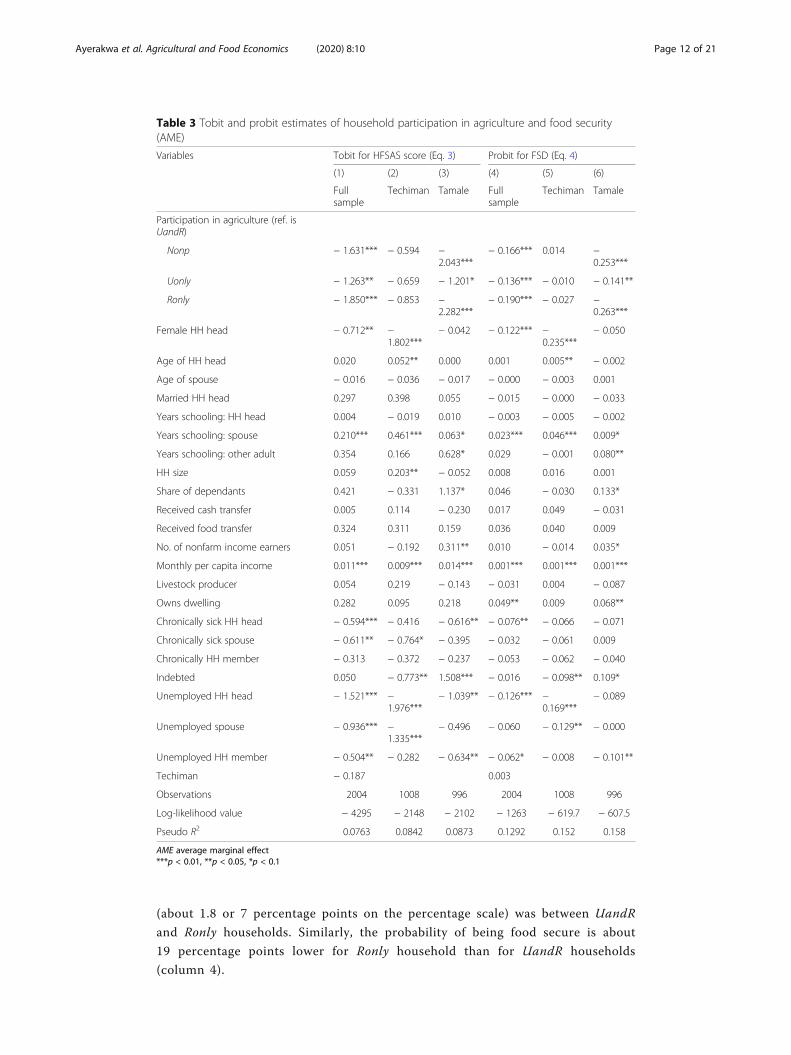
(about 1.8 or 7 percentage points on the percentage scale) was between UandR

and Ronly households. Similarly, the probability of being food secure is about

19 percentage points lower for Ronly household than for UandR households

(column 4).

Table 3 Tobit and probit estimates of household participation in agriculture and food security(AME)

Variables Tobit for HFSAS score (Eq. 3) Probit for FSD (Eq. 4)

(1) (2) (3) (4) (5) (6)

Fullsample

Techiman Tamale Fullsample

Techiman Tamale

Participation in agriculture (ref. isUandR)

Nonp − 1.631*** − 0.594 −2.043***

− 0.166*** 0.014 −0.253***

Uonly − 1.263** − 0.659 − 1.201* − 0.136*** − 0.010 − 0.141**

Ronly − 1.850*** − 0.853 −2.282***

− 0.190*** − 0.027 −0.263***

Female HH head − 0.712** −1.802***

− 0.042 − 0.122*** −0.235***

− 0.050

Age of HH head 0.020 0.052** 0.000 0.001 0.005** − 0.002

Age of spouse − 0.016 − 0.036 − 0.017 − 0.000 − 0.003 0.001

Married HH head 0.297 0.398 0.055 − 0.015 − 0.000 − 0.033

Years schooling: HH head 0.004 − 0.019 0.010 − 0.003 − 0.005 − 0.002

Years schooling: spouse 0.210*** 0.461*** 0.063* 0.023*** 0.046*** 0.009*

Years schooling: other adult 0.354 0.166 0.628* 0.029 − 0.001 0.080**

HH size 0.059 0.203** − 0.052 0.008 0.016 0.001

Share of dependants 0.421 − 0.331 1.137* 0.046 − 0.030 0.133*

Received cash transfer 0.005 0.114 − 0.230 0.017 0.049 − 0.031

Received food transfer 0.324 0.311 0.159 0.036 0.040 0.009

No. of nonfarm income earners 0.051 − 0.192 0.311** 0.010 − 0.014 0.035*

Monthly per capita income 0.011*** 0.009*** 0.014*** 0.001*** 0.001*** 0.001***

Livestock producer 0.054 0.219 − 0.143 − 0.031 0.004 − 0.087

Owns dwelling 0.282 0.095 0.218 0.049** 0.009 0.068**

Chronically sick HH head − 0.594*** − 0.416 − 0.616** − 0.076** − 0.066 − 0.071

Chronically sick spouse − 0.611** − 0.764* − 0.395 − 0.032 − 0.061 0.009

Chronically HH member − 0.313 − 0.372 − 0.237 − 0.053 − 0.062 − 0.040

Indebted 0.050 − 0.773** 1.508*** − 0.016 − 0.098** 0.109*

Unemployed HH head − 1.521*** −1.976***

− 1.039** − 0.126*** −0.169***

− 0.089

Unemployed spouse − 0.936*** −1.335***

− 0.496 − 0.060 − 0.129** − 0.000

Unemployed HH member − 0.504** − 0.282 − 0.634** − 0.062* − 0.008 − 0.101**

Techiman − 0.187 0.003

Observations 2004 1008 996 2004 1008 996

Log-likelihood value − 4295 − 2148 − 2102 − 1263 − 619.7 − 607.5

Pseudo R2 0.0763 0.0842 0.0873 0.1292 0.152 0.158

AME average marginal effect***p < 0.01, **p < 0.05, *p < 0.1


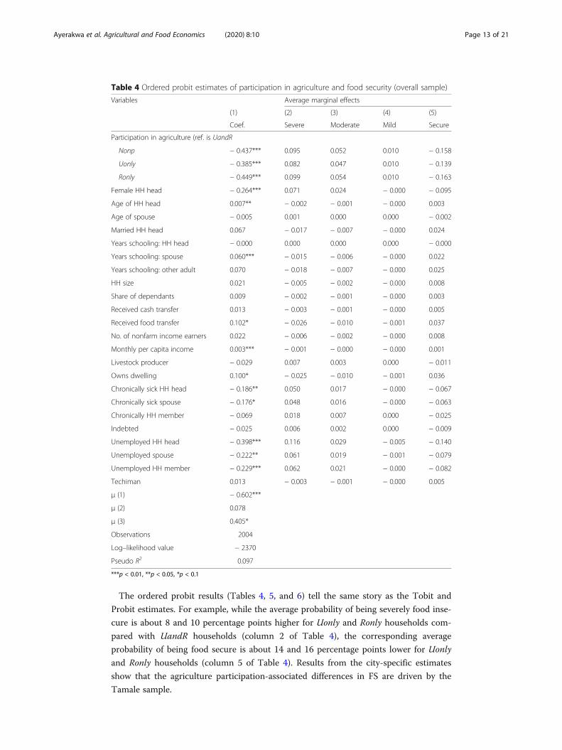
The ordered probit results (Tables 4, 5, and 6) tell the same story as the Tobit and

Probit estimates. For example, while the average probability of being severely food inse-

cure is about 8 and 10 percentage points higher for Uonly and Ronly households com-

pared with UandR households (column 2 of Table 4), the corresponding average

probability of being food secure is about 14 and 16 percentage points lower for Uonly

and Ronly households (column 5 of Table 4). Results from the city-specific estimates

show that the agriculture participation-associated differences in FS are driven by the

Tamale sample.

Table 4 Ordered probit estimates of participation in agriculture and food security (overall sample)

Variables Average marginal effects

(1) (2) (3) (4) (5)

Coef. Severe Moderate Mild Secure

Participation in agriculture (ref. is UandR

Nonp − 0.437*** 0.095 0.052 0.010 − 0.158

Uonly − 0.385*** 0.082 0.047 0.010 − 0.139

Ronly − 0.449*** 0.099 0.054 0.010 − 0.163

Female HH head − 0.264*** 0.071 0.024 − 0.000 − 0.095

Age of HH head 0.007** − 0.002 − 0.001 − 0.000 0.003

Age of spouse − 0.005 0.001 0.000 0.000 − 0.002

Married HH head 0.067 − 0.017 − 0.007 − 0.000 0.024

Years schooling: HH head − 0.000 0.000 0.000 0.000 − 0.000

Years schooling: spouse 0.060*** − 0.015 − 0.006 − 0.000 0.022

Years schooling: other adult 0.070 − 0.018 − 0.007 − 0.000 0.025

HH size 0.021 − 0.005 − 0.002 − 0.000 0.008

Share of dependants 0.009 − 0.002 − 0.001 − 0.000 0.003

Received cash transfer 0.013 − 0.003 − 0.001 − 0.000 0.005

Received food transfer 0.102* − 0.026 − 0.010 − 0.001 0.037

No. of nonfarm income earners 0.022 − 0.006 − 0.002 − 0.000 0.008

Monthly per capita income 0.003*** − 0.001 − 0.000 − 0.000 0.001

Livestock producer − 0.029 0.007 0.003 0.000 − 0.011

Owns dwelling 0.100* − 0.025 − 0.010 − 0.001 0.036

Chronically sick HH head − 0.186** 0.050 0.017 − 0.000 − 0.067

Chronically sick spouse − 0.176* 0.048 0.016 − 0.000 − 0.063

Chronically HH member − 0.069 0.018 0.007 0.000 − 0.025

Indebted − 0.025 0.006 0.002 0.000 − 0.009

Unemployed HH head − 0.398*** 0.116 0.029 − 0.005 − 0.140

Unemployed spouse − 0.222** 0.061 0.019 − 0.001 − 0.079

Unemployed HH member − 0.229*** 0.062 0.021 − 0.000 − 0.082

Techiman 0.013 − 0.003 − 0.001 − 0.000 0.005

μ (1) − 0.602***

μ (2) 0.078

μ (3) 0.405*

Observations 2004

Log–likelihood value − 2370

Pseudo R2 0.097

***p < 0.01, **p < 0.05, *p < 0.1


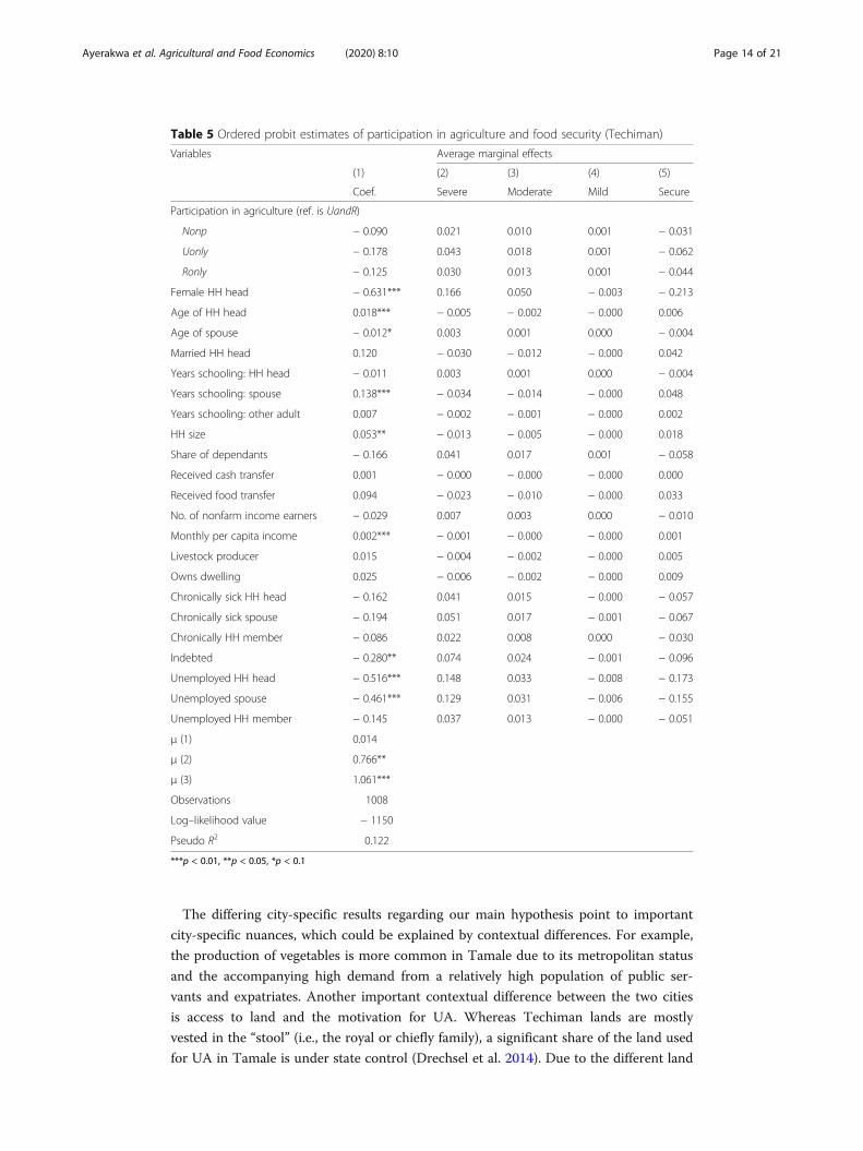
The differing city-specific results regarding our main hypothesis point to important

city-specific nuances, which could be explained by contextual differences. For example,

the production of vegetables is more common in Tamale due to its metropolitan status

and the accompanying high demand from a relatively high population of public ser-

vants and expatriates. Another important contextual difference between the two cities

is access to land and the motivation for UA. Whereas Techiman lands are mostly

vested in the “stool” (i.e., the royal or chiefly family), a significant share of the land used

for UA in Tamale is under state control (Drechsel et al. 2014). Due to the different land

Table 5 Ordered probit estimates of participation in agriculture and food security (Techiman)


(1) (2) (3) (4) (5)


Participation in agriculture (ref. is UandR)

Nonp − 0.090 0.021 0.010 0.001 − 0.031

Uonly − 0.178 0.043 0.018 0.001 − 0.062

Ronly − 0.125 0.030 0.013 0.001 − 0.044

Female HH head − 0.631*** 0.166 0.050 − 0.003 − 0.213

Age of HH head 0.018*** − 0.005 − 0.002 − 0.000 0.006

Age of spouse − 0.012* 0.003 0.001 0.000 − 0.004

Married HH head 0.120 − 0.030 − 0.012 − 0.000 0.042

Years schooling: HH head − 0.011 0.003 0.001 0.000 − 0.004

Years schooling: spouse 0.138*** − 0.034 − 0.014 − 0.000 0.048

Years schooling: other adult 0.007 − 0.002 − 0.001 − 0.000 0.002

HH size 0.053** − 0.013 − 0.005 − 0.000 0.018

Share of dependants − 0.166 0.041 0.017 0.001 − 0.058

Received cash transfer 0.001 − 0.000 − 0.000 − 0.000 0.000

Received food transfer 0.094 − 0.023 − 0.010 − 0.000 0.033

No. of nonfarm income earners − 0.029 0.007 0.003 0.000 − 0.010


Livestock producer 0.015 − 0.004 − 0.002 − 0.000 0.005

Owns dwelling 0.025 − 0.006 − 0.002 − 0.000 0.009

Chronically sick HH head − 0.162 0.041 0.015 − 0.000 − 0.057

Chronically sick spouse − 0.194 0.051 0.017 − 0.001 − 0.067


Indebted − 0.280** 0.074 0.024 − 0.001 − 0.096

Unemployed HH head − 0.516*** 0.148 0.033 − 0.008 − 0.173

Unemployed spouse − 0.461*** 0.129 0.031 − 0.006 − 0.155

Unemployed HH member − 0.145 0.037 0.013 − 0.000 − 0.051

μ (1) 0.014

μ (2) 0.766**

μ (3) 1.061***

Observations 1008


Pseudo R2 0.122

***p < 0.01, **p < 0.05, *p < 0.1


ownership arrangements, the motivation for UA in the two cities also differs. Farming

in urban Techiman is seen essentially as a strategy for ensuring land tenure security

while UA in Tamale is motivated more by the commercial motive as households devote

substantial amounts of resources to the production of vegetables for consumption and

sale to other urbanites.

The qualitative interviews also show that crop production by women, particu-

larly vegetables used in the preparation of local dishes, is encouraged around

homes in Tamale. This provides women the opportunity to work on the farm

Table 6 Ordered probit estimates of participation in agriculture and food security (Tamale)


(1) (2) (3) (4) (5)


Participation in agriculture (ref. is UandR)

Nonp − 0.609*** 0.128 0.069 0.018 − 0.216

Uonly − 0.388** 0.073 0.048 0.016 − 0.137

Ronly − 0.612*** 0.129 0.070 0.018 − 0.217

Female HH head − 0.053 0.014 0.005 0.000 − 0.019

Age of HH head 0.000 − 0.000 − 0.000 − 0.000 0.000

Age of spouse − 0.004 0.001 0.000 0.000 − 0.001

Married HH head − 0.032 0.008 0.003 0.000 − 0.011

Years schooling: HH head 0.004 − 0.001 − 0.000 − 0.000 0.002

Years schooling: spouse 0.017 − 0.004 − 0.002 − 0.000 0.006

Years schooling: other adult 0.177* − 0.045 − 0.017 − 0.001 0.063

HH size − 0.004 0.001 0.000 0.000 − 0.002

Share of dependants 0.217 − 0.055 − 0.020 − 0.001 0.077

Received cash transfer − 0.037 0.009 0.003 0.000 − 0.013

Received food transfer 0.052 − 0.013 − 0.005 − 0.000 0.018

No. of nonfarm income earners 0.092** − 0.023 − 0.009 − 0.001 0.033


Livestock producer − 0.106 0.027 0.010 0.000 − 0.037

Owns dwelling 0.114 − 0.029 − 0.011 − 0.001 0.041

Chronically sick HH head − 0.173 0.046 0.015 − 0.000 − 0.061

Chronically sick spouse − 0.139 0.037 0.012 0.000 − 0.049


Indebted 0.365** − 0.082 − 0.040 − 0.009 0.130

Unemployed HH head − 0.305* 0.085 0.023 − 0.003 − 0.106

Unemployed spouse − 0.014 0.004 0.001 0.000 − 0.005

Unemployed HH member − 0.304*** 0.083 0.025 − 0.001 − 0.107

μ (1) − 1.013***

μ (2) − 0.362

μ (3) 0.015

Observations 996


Pseudo R2 0.109

***p < 0.01, **p < 0.05, *p < 0.1


while carrying out reproductive activities (cooking and caring for children),

allowing men to commute to rural areas to farm. This result corroborates with

the finding of Maxwell (1995) that UA allowed women to combine productive

and child caregiving roles in Kampala. Indeed, according to our in-depth inter-

views, men in Tamale sometimes migrate temporarily to rural areas during the

rainy reason to access more land for the production of staple crops while

women and children cultivate the home gardens in the city.

We find other important predictors of urban household food security. In the interest of

brevity, we focus the discussion on results in Table 3. The significant predictors in the full

sample are sex of household head, women’s education, income, and idiosyncratic shocks

such as chronic illness and unemployment. Our results support findings in some of the

existing FS literature that female-headed households are less likely to be food secure than

male-headed households (Dzanku and Sarpong 2010; Bashir et al. 2012).

The significant gender difference, however, pertains to Techiman. For example, the esti-

mated average probability of being food secure is about 23 percentage points lower for

those living in female-headed households in Techiman compared with those living in

male-headed households in that city. Women are key influencers in meeting household

food and nutrition needs (Quisumbing et al. 1996; Rosegrant and Cline 2003). Mother’s

education level is particularly highly correlated with household FS in Techiman—an extra

year of schooling by a mother is estimated to raise the average probability of being food

secure by approximately 5 percentage points in Techiman; household head’s educational

level does not have a similar effect, however.

Income is important for achieving FS though the market arm as shown in the concep-

tual model. This is particularly important for urban households who are expected to rely

more on food markets for meeting their food needs. As expected, income is positively cor-

related with FS in both cities. In the full sample, increasing per capita income by an extra

$10 monthly is estimated to increase the probability of being food secure by 1% point.

Nonfarm employment seems more important for household food security in Tamale

where an extra household member employed in a nonfarm activity is estimated to raise

the probability of being food secure by approximately 3 percentage points. Owusu et al.

(2011) provides similar evidence for rural communities in northern Ghana.

We find household-specific health and unemployment events to have very negative

food security implications. For example, the presence of a chronically ill household

head is estimated to reduce household average FS score by about 2 percentage points

in the full sample; the presence of a chronically ill spouse carries an identical average

FS reducing effect. Being indebted has contrasting FS effects in the two cities—a nega-

tive effect in Techiman but a positive effect in Tamale. In theory, borrowing is not ne-

cessarily a negative thing, it depends on how the borrowed funds are utilized.

Robustness checksOne could worry about whether the result that urban households who participated in

agriculture in both urban and rural areas are more food secure is driven by endogeneity

bias, not least as a result of omitted variable bias and/or reverse causality. First, omitted

variable bias could arise through unobserved heterogeneity for which we need panel

data to address and as such is a weakness of this study, as it is for all cross-sectional ob-

servational data.


In the case of reverse causality, the key question is whether UandR households are more

food secure because they produce in rural and urban areas or they are so because their in-

dividual characteristics that allows them to participate in both spaces make them less

likely to be food insecure. This proposition is possible but unlikely for these urban house-

holds. First, as we have seen through the conceptual model, urban households do not

need to engage in agriculture to be food secure ex ante. Second, Table 2 shows that

UandR households are not the richest in terms of money matric indicators of welfare.

They also have the least access to financial services, which is very low in the sample. The

key endowments that are greater among UandR households than Nonp and Uonly house-

holds are household labor and livestock, which are control variables in the FS regressions.

However, as an econometric robustness check, we account for the possibility of en-

dogenous selection as follows. We first estimate a multinomial logit model to predict the

geography of agriculture participation. That is, we obtain Inverse Mills Ratios (IMRs) from

regressing prodloc, which is the nominal agriculture participation indicator, on all exogen-

ous variables, including identification variables or instruments. We then enter the IMRs

into the FS equations to correct for potential endogeneity bias in the spirit of Heckman

(1979).3 We use birthplace and parents occupation (full time farmer) as identifying vari-

ables. Being an indigene increases the likelihood of access to land for farming while par-

ents’ engagement in agriculture predicts current participation strongly in our data. We

bootstrap the standard errors due the two-step nature of the procedure. Test for joint sig-

nificance of the IMRs in the FS equations provides a test for endogeneity bias.

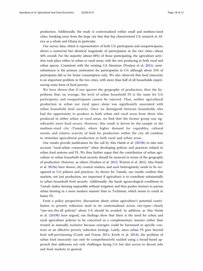
In the interest of brevity, we present the endogeneity corrected results for Eqs.

(3) and (4) in Appendix Table 7. First, we note that none of the IMRs are indi-

vidually significantly different from zero at even the 10% level. Second, the joint F

tests all yield p values that are larger than 0.10. With respect to the substantive re-

sults, we see that while our conclusions remain generally valid, correcting for po-

tential endogeneity leads to slightly imprecise point estimates. For example, UandR

households are only significantly more food secure than Nonp households at the

10% level (Appendix Table 7, column 3). Our results should thus be interpreted

with these issues in mind.

ConclusionThe received literature on the association between UA and FS has either focused on

urban household’s participation in agriculture irrespective of where the activity takes

place, or restricted participation to production within urban and peri-urban areas, or

more narrowly, production within build-up urban spaces. A recent systematic review of

the UA literature (Abu Hatab et al. 2019b) pointed to the need to fill an important gap

in the literature related to the role of rural-urban linkages, inter alia, in our understand-

ing of urban food systems and urban FS. This article is, in part, a response to this call

as it contributes to the UA literature by distinguishing between urban households’ agri-

cultural production activities in urban and rural areas and the implications for urban

household FS. By disentangling urban household’s participation in agriculture by geog-

raphy of production activities, we have been able to pick up food security implications

that would have been lost through an aggregation that ignores the geography of

3See Harou et al. (2016) for a more recent application of our approach.


production. Additionally, the study is contextualized within small and medium-sized

cities, breaking away from the large city bias that has characterized UA research in Af-

rica as a whole and Ghana in particular.

Our survey data, which is representative of both UA participants and nonparticipants,

shows a nontrivial but identical magnitude of participation in the two cities—about

44% overall. For the majority (about 88%) of those participating, the agriculture activ-

ities took place either in urban or rural areas, with the rest producing in both rural and

urban spaces. Consistent with the existing UA literature (Poulsen et al. 2015), semi-

subsistence is the primary motivation for participation in UA although about 35% of

participants did so for home consumption only. We also observed that food insecurity

is an important problem in the two cities, with more than half of all households experi-

encing some form of food poverty.

We have shown that if one ignores the geography of production, then the hy-

pothesis that, on average, the level of urban household FS is the same for UA

participants, and nonparticipants cannot be rejected. Thus, neither agricultural

production in urban nor rural space alone was significantly associated with

urban household food security. Once we distinguish between households who

had the opportunity to produce in both urban and rural areas from those who

produced in either urban or rural areas, we find that the former group was sig-

nificantly more food secure. However, this result is driven by the sample in the

medium-sized city (Tamale), where higher demand for vegetables, cultural

norms, and relative scarcity of land for production within the city all combine

to stimulate agricultural production in both rural and urban areas.

Our results provide justification for the call by Abu Hatab et al. (2019b) to take into

account “rural-urban connectivity” when developing policies and practices related to

urban food systems and FS. We thus further argue that the contribution of urban agri-

culture to urban household food security should be nuanced in terms of the geography

of production. However, as others (Poulsen et al. 2015; Warren et al. 2015; Abu Hatab

et al. 2019a) have shown, city context matters, and such heterogeneity needs to be rec-

ognized in UA policies and practices. As shown for Tamale, our results confirm that

markets, not just production, are important if agriculture is to contribute substantially

to urban household food security. Additionally, the harsh agroecological conditions in

Tamale makes farming impossible without irrigation and thus pushes farmers to pursue

urban farming in a more modern manner than in Techiman, which seems to result in

better FS.

From a policy perspective, discussions about urban agriculture’s potential contri-

bution to poverty reduction need to be contextualized across city-types—clearly

“one-size-fits-all policies” about UA should be avoided. In addition, as Abu Hatab

et al. (2019b) have argued, our findings show that there is the need for urban and

rural agriculture policies to be conceived in a complementary manner rather than

treated as mutually exclusive because synergies could be harnessed in specific con-

texts as an effective poverty reduction strategy. Lastly, since urban FS goes beyond

food self-provisioning (Crush and Frayne 2011; Korth et al. 2014), the problem of

urban food insecurity can only be comprehensively tackled using a broad-based ap-

proach that addresses not only challenges facing UA but also access to decent jobs

and food markets in general.


AcknowledgementsThe authors would like to thank AFSUN for permission to use portions of the AFSUN Household Food SecurityBaseline Survey instrument for the research. Special thanks to Professors Agnes Andersson Djurfeldt and MagnusJirström for their useful comments on the initial draft of the manuscript. We thank the two anonymous reviewers andthe editor who also provided very useful comments and suggestions that have helped improve the final output.

AppendixTable 7 Endogeneity corrected estimates of household participation in agriculture and FS (AME)

Variables Tobit for HFSAS score (Eq. 3) Probit for FSD (Eq. 4)

(1) (2) (3) (4) (5) (6)

Overall Techiman Tamale Full sample Techiman Tamale

Participation in agriculture(ref. is UandR)

Nonp − 1.474** − 0.756 − 1.635* − 0.177*** − 0.015 − 0.257***

Uonly − 1.135** − 0.675 − 0.742* − 0.136** − 0.011 − 0.121**

Ronly − 1.756*** − 0.830 − 2.058*** − 0.191*** − 0.028 − 0.258***

Female HH head − 1.732 − 2.282*** 0.351 − 0.258 − 0.300*** − 0.030

Age of HH head − 0.023 0.044 0.001 − 0.003 0.005 − 0.002

Age of spouse 0.003 − 0.034 − 0.007 0.002 − 0.002 0.002

Married HH head − 0.043 0.458 0.088 − 0.043 0.025 − 0.016

Years schooling: HH head − 0.116 − 0.041 0.014 − 0.015 − 0.006 − 0.001

Years schooling: spouse 0.382* 0.517*** 0.120 0.043 0.053*** 0.016

Years schooling: adult 0.157 0.461 0.655 0.013 0.038 0.085

HH size − 0.037 0.189* − 0.140* − 0.004 0.012 − 0.009

Share of dependants 1.681 0.513 1.904** 0.172 0.036 0.205**

Received cash transfer − 0.643 − 0.019 − 0.401 − 0.056 0.025 − 0.077

Received food transfer 0.663 0.366 − 0.015 0.072 0.050 − 0.005

No. of nonfarm income earners 0.293 − 0.273 0.373 0.036 − 0.026 0.044

Monthly per capita income 0.009** 0.009*** 0.014*** 0.001 0.001*** 0.001***

Livestock producer − 0.743 0.252 − 0.073 − 0.105 0.018 − 0.061

Owns dwelling − 0.164 − 0.449 0.261 0.003 − 0.048 0.071*

Chronically sick HH head − 0.359 − 0.432 − 0.569 − 0.057 − 0.069 − 0.075

Chronically sick spouse − 0.535* − 0.879** − 0.354 − 0.029 − 0.080 0.009

Chronically HH member − 0.392 − 0.075 − 0.102 − 0.063* − 0.019 − 0.021

Indebted − 0.818 − 0.891** 1.743 − 0.111 − 0.100 0.122

Unemployed HH head − 1.568*** − 2.234 − 1.093* − 0.133*** − 0.416 − 0.093

Unemployed spouse − 1.474* − 1.931 − 0.445 − 0.142 − 0.416 0.002

Unemployed HH member 0.881 0.055 − 0.329 0.077 0.011 − 0.070

Techiman 0.119 0.034

Correction terms

IMR1 0.123 0.223 − 0.170 0.011 0.025 − 0.019

IMR2 − 0.518 − 0.210 0.003 − 0.056 − 0.023 − 0.004

IMR3 0.376 − 0.015 0.113 0.039 − 0.006 0.012

Joint F-stat for IMRs 0.630 0.261 1.994 0.615 0.310 1.784

P-value of F-test 0.595 0.854 0.113 0.605 0.818 0.149

Observations 2004 1008 996 2004 1008 996

Log-likelihood value − 4295 − 2148 − 2102 − 1263 − 619.7 − 607.5

Pseudo R2 0.081 0.087 0.089 0.128 0.161 0.163

AME average marginal effect***p < 0.01, **p < 0.05, *p < 0.1


Authors’ contributionsHMA conceived the main research question addressed in the article. He also participated in data collection,contributed to data analysis, and produced the initial draft of the manuscript. FMD was a co-principal investigator ofthe project in Ghana and led the data collection. He developed the analytical framework for the current article andcarried out the statistical and econometric analyses and interpretation of results. He also produced the final draft ofthe manuscript. DBS was a co-principal investigator of the project in Ghana. He provided comments on an initial draftof the paper that led to the development of the initial manuscript. All authors approved the final manuscript.

FundingFunding for the Urban Agriculture Project was provided by the Swedish Research Council for Environment,Agricultural Sciences and Spatial Planning. This funding was provided under the Swedish African Urban AgricultureProject.

Availability of data and materialsThe data used for this article is currently not available publicly but could be made available upon request, withpermission from the project team leaders.

Competing interestsThe author(s) declare that they have no competing interests.

Author details1University of Ghana Learning Centres, School of Continuing and Distance Education, University of Ghana, Accra,Ghana. 2Institute of Statistical, Social and Economic Research (ISSER), University of Ghana, Accra, Ghana. 3Departmentof Agricultural Economics and Agribusiness, University of Ghana, Accra, Ghana.

Received: 29 July 2018 Accepted: 17 March 2020

ReferencesAbu Hatab A, Cavinato MER, Lagerkvist CJ (2019a) Urbanization, livestock systems and food security in developing countries:

a systematic review of the literature. Food Security 11(2):279–299Abu Hatab A, Cavinato MER, Lindemer A, Lagerkvist C-J (2019b) Urban sprawl, food security and agricultural systems in

developing countries: a systematic review of the literature. Cities 94:129–142Armar-Klemesu M (2000) Urban agriculture and food security, nutrition and health. In: Bakker N, Dubbeling M, Gundel S,

Sabel-Koschella U, de Zeeuw H (eds) Growing Cities, Growing Food, Urban Agriculture on the Policy Agenda. DSEFeldafing, Feldafing, Germany

Ayerakwa HM (2017) Urban households’ engagement in agriculture: implications for household food security in Ghana’smedium sized cities. Geographical Research 55(2):217–230

Badami MG, Ramankutty N (2015) Urban agriculture and food security: a critique based on an assessment of urban landconstraints. Global Food Security 4:8–15

Bashir, M. K., Schilizzi, S. & Pandit, R. (2012). The determinants of rural household food security in the Punjab, Pakistan: aneconometric analysis. Available:

Battersby J, Watson V (2019) Urban food systems governance and poverty in African cities. Routledge, London & New YorkBecquey E, Martin-Prevel Y, Traissac P, Dembélé B, Bambara A, Delpeuch F (2010) The household food insecurity access scale

and an index-member dietary diversity score contribute valid and complementary information on household foodinsecurity in an urban West-African setting. The Journal of nutrition 140(12):2233–2240

Bryld E (2003) Potentials, problems, and policy implications for urban agriculture in developing countries. Agric Human Values20(1):79–86

Burchi F, De Muro P (2016) From food availability to nutritional capabilities: advancing food security analysis. Food Policy 60:10–19

Clinton N, Stuhlmacher M, Miles A, Uludere Aragon N, Wagner M, Georgescu M, Herwig C, Gong P (2018) A global geospatialecosystem services estimate of urban agriculture. Earth's Future 6(1):40–60

Coates, J., Swindale, A. & Bilinsky, P. (2007). Household Food Insecurity Access Scale (HFIAS) for measurement of food access:indicator guide. Food and Nutrition Technical Assistance III Project (FANTA). Washington, DC. Available:

Crush J, Frayne B (2011) Supermarket expansion and the informal food economy in Southern African cities: implications forurban food security. J Southern Afr Studies 37(4):781–807

Crush J, Hovorka A, Tevera D (2011) Food security in southern African cities: the place of urban agriculture. Progress DevStudies 11(4):285–305

Drechsel P, Adam-Bradford A, Raschid-Sally L (2014) Irrigated urban vegetable production in Ghana: a farming systembetween challenges and resilience. In: Drechsel P, Keraita B (eds) Irrigated urban vegetable production in Ghana:characteristics, benefits and risk mitigation. International Water Management Institute (IWMI), Colombo, Sri Lanka, p 247

Dzanku F, Sarpong D (2010) Agricultural diversification, food self-sufficiency and food security in Ghana–the role ofinfrastructure and institutions. African Smallholder. Food Crops, Markets and Policy, CABI, Wallingford, UK, pp 189–213

Dzanku FM (2019) Food security in rural sub-Saharan Africa: exploring the nexus between gender, geography and off-farmemployment. World Dev 113:26–43

Ellis F, Sumberg J (1998) Food production, urban areas and policy responses. World Dev 26(2):213–225FAO (2009) Declaration of the World Food Summit on Food Security. Food and Agriculture Organization of the United Nations,

RomeFrayne B, McCordic C, Shilomboleni H (2014) Growing Out of Poverty: Does urban agriculture contribute to household food

security in Southern African cities? Urban Forum 25:177–189


Frelat R, Lopez-Ridaura S, Giller KE, Herrero M, Douxchamps S, Djurfeldt AA, Erenstein O, Henderson B, Kassie M, Paul BK,Rigolot C, Ritzema RS, Rodriguez D, van Asten PJA, van Wijk MT (2016) Drivers of household food availability in sub-Saharan Africa based on big data from small farms. Proc Natl Acad Sci 113(2):458–463

Gebreyesus SH, Lunde T, Mariam DH, Woldehanna T, Lindtjørn B (2015) Is the adapted Household Food Insecurity AccessScale (HFIAS) developed internationally to measure food insecurity valid in urban and rural households of Ethiopia? BMCNutrition 1(1):1

Gerstl S, Cissé G, Tanner M (2002) The economic impact of urban agriculture on home gardeners in Ouagadougou. UrbanAgric Magazine 7:12–15

Ghana Statistical Service (2014a) 2010 population and housing census: district analytical report: Tamale Metropolis. GhanaStatistical Service, Accra, Ghana

Ghana Statistical Service (2014b) 2010 population and housing census: district analytical report: Techiman Municipality. GhanaStatistical Service, Accra, Ghana

Harou AP, Walker TF, Barrett CB (2016) Is late really better than never? The farmer welfare effects of pineapple adoption inGhana. Agric Econ:1–12

Headey D, Ecker O (2013) Rethinking the measurement of food security: from first principles to best practice. Food Security5(3):327–343

Heckman JJ (1979) Sample selection bias as a specification error. Econometrica 47(1):153–161Korth M, Stewart R, Langer L, Madinga N, Da Silva NR, Zaranyika H, van Rooyen C, de Wet T (2014) What are the impacts of

urban agriculture programs on food security in low and middle-income countries: a systematic review. Environ Evidence3(1):21

Lee-Smith D (2010) Cities feeding people: an update on urban agriculture in equatorial Africa. Environ Urbanization 22(2):483–499

Lee-Smith D (2013) Which way for UPA in Africa? City 17(1):69–84Maxwell D (2001) The importance of urban agriculture to food and nutrition. Annotated biography, ETC-RUAF. CTA

publishers, Leusden, NetherlandsMaxwell DG (1995) Alternative food security strategy: a household analysis of urban agriculture in Kampala. World Dev 23(10):

1669–1681MoFA (2010). Medium Term Agriculture Sector Investment Plan (METASIP): 2011-2015. Ministry of Food and Agriculture.Mougeot L (2000) Achieving urban food and nutrition security in developing countries: the hidden significance of urban

agriculture. IFPRI, Brief paper 6Mougeot, L. J. (2005). Agropolis: the social, political, and environmental dimensions of urban agriculture. IDRC.Mougeot LJ (2006) Growing better cities: urban agriculture for sustainable development. IDRC, OttawaNugent R (2000) The impact of urban agriculture on the household and local economies. In: Bakker N, Dubbeling M, Gündel

S, Sabel-Koshella U, de Zeeuw H (eds) Growing cities, growing food. Urban agriculture on the policy agenda. Zentralstelle fürErnährung und Landwirtschaft (ZEL), Feldafing, Germany, pp 67–95

Owusu V, Abdulai A, Abdul-Rahman S (2011) Non-farm work and food security among farm households in Northern Ghana.Food Policy 36(2):108–118

Poulsen MN, McNab PR, Clayton ML, Neff RA (2015) A systematic review of urban agriculture and food security impacts inlow-income countries. Food Policy 55:131–146

Quisumbing AR, Brown LR, Feldstein HS, Haddad L, Peña C (1996) Women: the key to food security. Food Nutr Bull 17(1):1–2Rogerson CM (2003) Towards “pro-poor” urban development in South Africa: the case of urban agriculture. Acta Academica 1:

130–158Rosegrant MW, Cline SA (2003) Global food security: challenges and policies. Science 302(5652):1917–1919Salarkia N, Abdollahi M, Amini M, Neyestani TR (2014) An adapted Household Food Insecurity Access Scale is a valid tool as a

proxy measure of food access for use in urban Iran. Food Security 6(2):275–282Shifa M, Borel-Saladin J (2019) African urbanisation and poverty. In: Battersby J, Watson V (eds) Urban Food Systems

Governance and Poverty in African Cities. Routledge, London & New YorkSmit W (2016) Urban governance and urban food systems in Africa: examining the linkages. Cities 58:80–86Stewart R, Korth M, Langer L, Rafferty S, Da Silva N, van Rooyen C (2013) What are the impacts of urban agriculture programs

on food security in low and middle–income countries? Environ Evidence 2(7):1–13Tukolske C, Andam KS, Blekking J, Evans T, Caylor K (2018) Measures and determinants of urban food security: evidence from

Accra, Ghana. GSSP Working Paper 50. International Food Policy Research Institute, Washington, D.C. Available: http://ebrary.ifpri.org/cdm/ref/collection/p15738coll2/id/132944

Warren E, Hawkesworth S, Knai C (2015) Investigating the association between urban agriculture and food security, dietarydiversity, and nutritional status: a systematic literature review. Food Policy 53:54–66

Weidner T, Yang A, Hamm MW (2019) Consolidating the current knowledge on urban agriculture in productive urban foodsystems: learnings, gaps and outlook. J Cleaner Production 209:1637–1655

Yamane, T. (1967). Problems to accompany “Statistics, an introductory analysis”, 2nd edition. Harper & Row.Zezza A, Tasciotti L (2010) Urban agriculture, poverty, and food security: empirical evidence from a sample of developing

countries. Food Policy 35(4):265–273

Publisher’s NoteSpringer Nature remains neutral with regard to jurisdictional claims in published maps and institutional affiliations.


http://ebrary.ifpri.org/cdm/ref/collection/p15738coll2/id/132944

http://ebrary.ifpri.org/cdm/ref/collection/p15738coll2/id/132944

Documents

The geography of agriculture participation and food