The geographic scaling of biotic interactions - PeerJ · 1" " 1" The geographic scaling of 2" biotic interactions 3" Miguel B. Araújo1,2,3,4* & Alejandro Rozenfeld3* 4" 1Imperial

1

The geographic scaling of 1

biotic interactions 2

Miguel B. Araújo1,2,3,4* & Alejandro Rozenfeld3* 3 1Imperial College London, Silwood Park Campus, Buckhurst Road, Ascot SL5 7PY, Berks, United Kingdom 4 ([email protected]) 5 2Department of Biogeography and Global Change, National Museum of Natural Sciences, CSIC, Calle José Gutiérrez 6 Abascal, 2, 28006, Madrid, Spain 7 3‘Rui Nabeiro’ Biodiversity Chair, CIBIO, University of Évora, Largo dos Colegiais, 7000 Évora, Portugal 8 4Center for Macroecology, Evolution and Climate, University of Copenhagen, 2100 Copenhagen, Universitetsparken 9 15, 2100, Denmark 10 * Authors contributed equally 11

12

Abstract: A central tenet of ecology and biogeography is that the broad outlines of 13

species ranges are determined by climate, whereas the effects of biotic interactions are 14

manifested at local scales. While the first proposition is supported by ample evidence, 15

the second is still a matter of controversy. To address this question, we develop a 16

mathematical model that predicts the spatial overlap, i.e., co-occurrence, between pairs 17

of species subject to all possible types of interactions. We then identify the scale in 18

which predicted range overlaps are lost. We found that co-occurrence arising from 19

positive interactions, such as mutualism (+/+) and commensalism (+/0), are manifested 20

across scales of resolution. Negative interactions, such as competition (-/-) and 21

amensalism (-/0), generate checkerboard-type co-occurrence patterns that are 22

discernible at finer resolutions. Scale dependence in consumer-resource interactions (+/-23

) depends on the strength of positive dependencies between species. Our results 24

challenge the widely held view that climate alone is sufficient to characterize species 25

distributions at broad scales, but also demonstrate that the spatial signature of 26

competition is unlikely to be discernible beyond local and regional scales. 27

28

29

30

31

32 PeerJ PrePrints | https://peerj.com/preprints/82v1/ | v1 received: 17 Oct 2013, published: 17 Oct 2013, doi: 10.7287/peerj.preprints.82v1

PrePrin

ts

2

Introduction 33

The question of whether the geographical ranges of species are determined by their 34

ecological requirements and the physical characteristics of individual sites, or by 35

assembly rules reflecting interactions between species, has long been a central issue in 36

ecology (e.g., Andrewartha and Birch 1954, Diamond 1975, Gotelli and Graves 1996, 37

Chase and Leibold 2003, Peterson et al. 2011). Evidence is compelling that the limits of 38

species ranges often match combinations of climate variables, especially at high 39

latitudes and altitudes (e.g., Grinnell 1917, Andrewartha and Birch 1954, Hutchinson 40

1957, Woodward 1987, Root 1988), and that these limits shift through time in 41

synchrony with changes in climate (e.g., Walther et al. 2005, Hickling et al. 2006, 42

Lenoir et al. 2008). However, recent evidence suggests that the thermal component of 43

species climatic niches is more similar among terrestrial organisms than typically 44

expected (Araújo et al. 2013), leading to the conclusion that spatial turnover among 45

distributions of species might often result from non-climatic factors (see also for 46

discussion Baselga et al. 2012a). The degree to which non-climatic factors shape the 47

distributions of species has been focus of discussion in community ecology and 48

biogeography for over a century, with several authors proposing that climate exerts 49

limited influence at lower latitudes and altitudes (e.g., Wallace 1878, Dobzhansky 1950, 50

Loehle 1998, Svenning and Skov 2004, Colwell et al. 2008, Baselga et al. 2012b). 51

Specifically, much interest exists regarding the extent to which occurrences of species 52

are constrained by the distributions of other species at broad scales of resolution and 53

extent (e.g., Gravel et al. 2011). It has been argued that biotic interactions determine 54

whether species thrives or withers in a given environment, but that the spatial effects 55

associated with these interactions are lost at broad scales (e.g., Whittaker et al. 2001, 56

Pearson and Dawson 2003, McGill 2010). In contrast, modelling studies have hinted 57

that biotic interactions could leave broad-scale imprints on coexistence and, therefore, 58

on species distributions (e.g., Araújo and Luoto 2007, Heikkinen et al. 2007, Meier et 59

al. 2010, Bateman et al. 2012). But empirical evidence for the broad scale effects of 60

biotic interactions is limited. A study has shown that with scales of few hundred 61

kilometres the effects of competition on geographical ranges can still be discernible 62

(Gotelli et al. 2010), but at scales of biomes such effects are often diluted (Russell et al. 63

2006, Veech 2006). How general are these patterns? 64

65

PeerJ PrePrints | https://peerj.com/preprints/82v1/ | v1 received: 17 Oct 2013, published: 17 Oct 2013, doi: 10.7287/peerj.preprints.82v1

PrePrin

ts

3

Empirical studies of the effects of biotic interactions on species distributions have 66

historically focused on competition (e.g., Gause 1934, Hardin 1960, MacArthur 1972, 67

Schoener 1982, Amarasekare 2003). However, several authors have pointed out that a 68

greater variety of interactions can control for spatial patterns of overlap between species 69

(e.g., Hairston et al. 1960, Connell 1975, Ricklefs 1987, Callaway et al. 2002, Bruno et 70

al. 2003, Travis et al. 2005, Ricklefs 2010). Competition is a specific case involving two 71

species that are worse off interacting with one another (which we annotate as: -/-). In its 72

extreme form, competition leads to co-exclusion of the interacting species (MacArthur 73

1972). The reverse of competition is mutualism, whereby two species display mutual 74

dependency (+/+). Different combinations of positive, negative, and neutral 75

relationships exist and they generate consumer-resource interactions such as predation, 76

herbivory, parasitism and disease (+/-), or amensalism (-/0) and commensalism (+/0). 77

78

The spatial effects of the different biotic interactions have rarely, if ever, been 79

investigated. Differences in patterns of co-occurrence arising from alternative biotic 80

interactions are seldom stated and focus has been on identifying non-random patterns of 81

co-occurrence between pairs of species (e.g., Gotelli and McCabe 2002, Horner-Devine 82

et al. 2007, Gotelli et al. 2010). Substantial controversy exists regarding the appropriate 83

null models in such analyses (for review and discussion see Gotelli and Graves 1996), 84

but the more fundamental question of whether departures from randomness in co-85

occurrence patterns provide interpretable information regarding the underlying biotic 86

interactions remains unanswered. 87

88

In practice, several biotic and abiotic factors can simultaneously affect the distributions 89

of species (e.g., Soberón 2010, Peterson et al. 2011) and, therefore, co-occurrence (e.g., 90

Cohen 1971, Leibold 1997, Amarasekare et al. 2004, Ovaskainen et al. 2010, Araújo et 91

al. 2011). One approach to disentangle the relative importance of factors causing 92

changes in species co-occurrence is through simulations (Urban 2005). Here, we 93

develop a novel ‘point-process’ model that infers co-occurrence of species across the 94

full space of potential biotic interactions between pairs of species: i.e., given all biotic 95

interaction types (+/+, +/-, -/-, +/0, -/0) and all possible combinations of biotic 96

interaction strength (0 ≤ 𝐼! ≤ 1) (for more details see material and methods). Dynamic 97

Lotka-Volterra-type models could also be used as they explicitly simulate the effects of 98

different biotic interactions on population dynamics (e.g., predation, competition, 99 PeerJ PrePrints | https://peerj.com/preprints/82v1/ | v1 received: 17 Oct 2013, published: 17 Oct 2013, doi: 10.7287/peerj.preprints.82v1

PrePrin

ts

4

mutualism, see for review Kot 2001). However, Lotka-Volterra models require detailed 100

parameterization of mortality and colonization rates that are highly contingent and are 101

usually impossible to obtain. Furthermore, models predicting the spatial effects of 102

repulsive and attractive interactions at steady state would be particularly useful if the 103

goal is to examine these spatial effects rather than the underlying population dynamics 104

that generate them (see also Dieckmann et al. 2000, Law and Dieckmann 2000). The 105

critical issue is whether a simple point-process model, such as ours, simulates spatial 106

patterns of co-occurrence comparable with dynamic Lotka-Volterra models at 107

equilibrium. Preliminary analysis comparing our model with Markov-chain formulation 108

of Lotka-Volterra models by Cohen (1970) supports this view and is being prepared for 109

publication elsewhere (Rozenfeld & Araújo, unpublished). 110

111

In the current implantation of the proposed point-process model, and to control for the 112

effects of species range sizes and environmental clustering on species distributions, 113

simulations were replicated for species ranges with varying prevalence and spatial 114

autocorrelation. Once co-occurrence between two species was estimated, we sampled 115

ranges at increasingly coarser scales of resolution (i.e., by increasing grid-cell size) and 116

identified the scale at which the original patterns of co-occurrences lost the signature of 117

the biotic interactions effects. When the effects of biotic interactions on patterns of co-118

occurrence of species were maintained across scales of resolution we interpreted the 119

pattern as providing evidence for scale independence. In contrast, biotic interactions 120

generating patterns of co-occurrence that were lost at increasing scales of resolutions 121

were interpreted as being strongly dependent on the scale. 122

123

Material and methods 124

The model 125

The primary assumption of our point-process model is that the signal of biotic 126

interactions drives spatial attraction (for +) or repulsion (for -). It follows that if no 127

interactions are present (0/0), co-occurrence between species ranges is dependent on 128

their prevalence (ρ=fraction of the sites where the species is present). Formally, if 129

species probabilities of occurrence are equal to their respective prevalence, i.e., 130

𝑃 𝐴 = 𝜌! and 𝑃 𝐵 = 𝜌!, then the probability of co-occurrence between ranges of 131

two non-interacting species is given by 132

𝑃!"## 𝐴 ∩ 𝐵 = 𝜌!𝜌! (1) 133 PeerJ PrePrints | https://peerj.com/preprints/82v1/ | v1 received: 17 Oct 2013, published: 17 Oct 2013, doi: 10.7287/peerj.preprints.82v1

PrePrin

ts

5

The probability of co-occurrence is the expected fraction of sites where species co-134

occur. If species A and B interact, then their overlap is a function of both their 135

prevalence and the strength of their interactions 𝐼! and 𝐼! 136

𝑃 𝐴 ∩ 𝐵 = 𝑓 𝜌!,𝜌! , 𝐼!, 𝐼! (2) 137

138

Interactions can be either attractive 𝐼!! or repulsive 𝐼!!, with 0 ≤ 𝐼! !" !! !" ! ≤ 1. It follows 139

that 𝐼!! stands for the intensity with which species A is attracted by B, and 𝐼!! is the 140

intensity with which species B is attracted by A. Likewise, 𝐼!! stands for the intensity 141

with which species A repulses B, and 𝐼!! is the intensity with which species B repulses 142

A. 143

144

In the particular case of mutualism (+/+), positive interactions will cause species to co-145

occur more often than expected under the null model 146

𝑃 !/! 𝐴 ∩ 𝐵 = 𝜌!𝜌! +max 𝐼!!, 𝐼!! ×[min (𝜌!,𝜌!)− 𝜌!𝜌!] (3) 147

Where the second term in equation 3 estimates the excess of co-occurrence due to 148

positive (+/+) interactions. The maximum fraction of sites where species co-occur is 149

limited by the prevalence of the species with the most restricted range, i.e., min (𝜌!,𝜌!). 150

So that [min (𝜌!,𝜌!)− 𝜌!𝜌!] refers to the maximum excess of co-occurrence over the 151

null model. With interactions (+/+), the species with the greatest positive dependence is 152

the one that constrains co-occurrence between the two interacting species. That is, the 153

maximum excess of co-occurrence is modulated by the maximum attracting index 154

(max 𝐼!!, 𝐼!! ). 155

So, 156

𝑃(!/!) 𝐴 ∩ 𝐵 = 𝜌!𝜌! 𝐼!! = 0 𝑎𝑛𝑑 𝐼!! = 0 min(𝜌!,𝜌!) 𝐼!! = 1 𝑜𝑟 𝐼!! = 1

When both interaction strengths are 0 we recover the null expectation, and when one of 157

the species is fully dependent on the other the co-occurrence range is maximal. 158

159

In the case of competition (-/-), negative interactions will cause the species to co-occur 160

less often than expected under the null model 161

𝑃(!/!) 𝐴 ∩ 𝐵 = 𝜌!𝜌!×[1−max 𝐼!!, 𝐼!! ] (4) 162

Co-occurrence will tend to zero as the interaction strength of at least one of the 163

interacting species approaches 1. With interactions (-/-), the species with the greatest 164


PrePrin

ts

6

negative (repulsive) interaction is the one that constrains co-occurrence between the two 165

interacting species. That is, co-occurrence decreases below the null expectation 166

proportionally to the maximum repulsion strength (max 𝐼!!, 𝐼!! ). 167

So, 168

𝑃(!/!) 𝐴 ∩ 𝐵 = 𝜌!𝜌! 𝐼!! = 0 𝑎𝑛𝑑 𝐼!! = 00 𝐼!! = 1 𝑜𝑟 𝐼!! = 1

When both interaction strengths are 0 we recover the null expectation and, when one of 169

the species is fully excluded by the other, co-occurrence is zero. 170

171

In the case of consumer-resource interactions (+/-) with A being the consumer and B the 172

resource, both positive and negative interactions will cause co-occurrence to deviates 173

from the null expectation 174

𝑃(!/!) 𝐴 ∩ 𝐵 = [𝜌!𝜌! + 𝐼!!× min (𝜌!,𝜌!)− 𝜌!𝜌! ]×(1− 𝐼!!) (5) 175

The equation 5 is a combination of equations 3 and 4. The first factor [𝜌!𝜌! +176

min (𝜌!,𝜌!)− 𝜌!𝜌! 𝐼!!] corresponds to equation 3 with 𝐼!! = 0, and it shows how co-177

occurrence is increased due to the positive dependence of species A on B. The second 178

factor (1− 𝐼!!) reduces co-occurrence proportionally to the repulsive strength (𝐼!!) . 179

So, 180

𝑃(!/!) 𝐴 ∩ 𝐵 =𝜌!𝜌! 𝐼!! = 0 𝑎𝑛𝑑 𝐼!! = 0

min (𝜌!,𝜌!) 𝐼!! = 1 𝑎𝑛𝑑 𝐼!! = 00 𝐼!! = 1

When both interaction strengths are 0 we recover the null expectation. When species A 181

is fully dependent on B and species B does not repulse A then the co-occurrence reaches 182

its maximum. Finally, when species B repulses A with maximum intensity co-183

occurrence is forbidden. 184

185

Notice that commensalism is a special case of mutualism (with 𝐼!! = 0) or predation, 186

parasitism and disease (with 𝐼!! = 0), while amensalism is a special case of competition 187

(with 𝐼!! = 0). By varying the sign (+, -) and the strength 𝐼! (0 ≤ 𝑥 ≤ 1), our model 188

predicts range overlaps across the full biotic interaction space. 189

190

Simulations 191

The general formulation of our point-process model defines rules of attraction and 192

repulsion among species subject to different biotic interaction types and strengths, but 193


PrePrin

ts

7

these interactions take place in non-heterogeneous landscapes where multiple drivers, in 194

addition to interactions, can affect species ranges and, therefore, co-occurrence. 195

Constraints to the general model can be added to take these drivers into account, such as 196

varying the ecological niches of species (both in the sense of species affecting and being 197

affected by the environment, e.g., Chase and Leibold 2003, Peterson et al. 2011), or 198

dispersal (both in the sense of species having the ability to disperse and being prevented 199

from it due to external barriers, e.g., Levin 1974, Pulliam 1988, Hanski 1998, 200

Humphries and Parenti 1999). Here, we explore two features of species ranges that we 201

deem relevant for studying the geographical scaling of biotic interactions. The first is 202

prevalence (ρ). In one implementation of the model, the prevalence of species is 203

relatively low: each species occupies 10% of the studied region (ρ=0.1). In the other 204

implementation of the model species occupy 30% (ρ=0.3) of the studied region. 205

206

The second feature explored is the placement of ranges. In one implementation of the 207

model, species B is randomly located and species A is constrained by species B. Under 208

this model, environmental conditions are assumed to be homogenous across the studied 209

area as it would be expected if range overlaps were measured within a given habitat 210

type. In such a scenario, species B can be found anywhere in geographical space and 211

range overlaps between species A and B are solely determined by prevalence and the 212

attractive and repulsive effects of interactions. In the modified model, the distribution of 213

species B is spatially structured while species A is a function of species B. This 214

implementation of the model simulates range overlaps when the distribution of one of 215

the species is highly autocorrelated (e.g., Legendre 1993, Dormann et al. 2007). Such 216

autocorrelation can arise because strong environmental gradients exist and act to 217

constrain species ranges (as might often occur at biogeographical extents) and/or when 218

dispersal, demographic or behavioural factors cause individuals to aggregate in specific 219

portions of geographical space (as might often occur at local and landscape extents). All 220

simulations were performed in lattices of 100x100 pixels. In order to account for 221

stochastic differences in the placement of the ranges, simulations were repeated 1000 222

times. Details on the generation of random and spatially autocorrelated distributions are 223

provided in the supporting online material, together with the Mat Lab computer code 224

written by AR and used to generate the species ranges (see supporting online material). 225

226


PrePrin

ts

8

Measuring spatial dependencies in biotic interactions 227

To address the question of how co-occurrences emerging from different biotic 228

interactions affect species distributions at different spatial resolutions we used a 229

hierarchical framework (Allen and Starr 1982). We compared co-occurrence scores 230

(measured as the ratio of the number of geographical cells where species A and B co-231

occur to the total number of occupied cells) at the original resolution used to fit all of 232

our models (the cell in our lattice landscape) with co-occurrences measured at 233

progressively larger scales of resolution. This hierarchical framework for scaling was 234

achieved by increasing the size of the blocks where individuals occur, and then 235

quantifying the resulting co-occurrence. The quantification of co-occurrence was done 236

using two approaches. The first seeks to preserve information about the ‘true’ co-237

occurrence of species that exists within geographical blocks and counts species as co-238

occurring if, and only if, they co-occur within one or more cell within the larger block. 239

The second emulates the traditional approach of ‘sampling’ species occurrences’ data in 240

macroecology (e.g., Rahbek and Graves 2001, McPherson et al. 2006, Nogués-Bravo 241

and Araújo 2006), and counts species as co-occurring if both species are present 242

somewhere in the block regardless of whether they co-exist in the cells. 243

244

The ‘true’ and ‘sampled’ co-occurrence scores measured at the cell level are then 245

plotted against progressively larger block sizes. The area between the curves 246

representing the ‘true’ and ‘sampled’ co-occurrence percentages between species A and 247

B, across the range of block sizes, provides a measure of scale dependence of co-248

occurrence patterns (see Figure 1). The greater the area between the two curves the 249

more the effects of given biotic interaction on species’ distributions depend on spatial 250

resolution, and vice versa (see Figure 1). The area between the ‘true’ and the ‘sampled’ 251

co-occurrences is calculated for the full set of possible biotic interactions that can arise 252

from combining interactions of varying signs (+, -) and strengths 𝐼! (0 ≤ 𝑥 ≤ 1). 253


PrePrin

ts

9

254

Figure 1 – Scale dependence of biotic interactions. Right (squared landscape): after the range 255

of species A and B have been simulated, co-occurrence between the two species is calculated. 256

Black squares indicate occurrence of species A but not species B, gray squares indicate 257

occurrence of B but not A, and red squares indicate co-occurrence of A and B. Left (diagram): 258

by progressively increasing the size of the squares, ‘sampling’ would lead to classifying species 259

has co-occurring if both occurred somewhere in the square (black line indicates ‘resampled’ co-260

occurrence), while species would only co-occur if species overlapped within the square (red line 261

indicates ‘true’ co-occurrence). The greater the area between the red and black lines the greater 262

the scale dependence of biotic interactions. 263

264

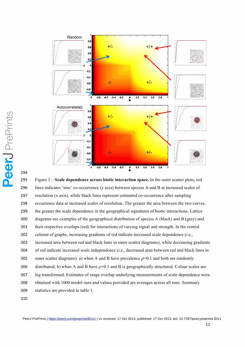
Results 265

Although positive interactions generate range overlaps and negative interactions 266

generate non-overlaps, equivalent degrees of overlap were recorded for species exposed 267

to different types of biotic interactions (Figure 2). For example, the spatial patterns of 268

range overlap for commensalism (𝐼!!, 𝐼!!) can be identical to range overlaps arising 269

from mutualistic interactions (𝐼!!, 𝐼!!) (Figure 1). Range overlaps from amensalism 270

(𝐼!!, 𝐼!!) can also mach range overlaps from competition (𝐼!!, 𝐼!!). Patterns of range 271

overlap from consumer-resource interactions (𝐼!!, 𝐼!!) can be like that of any type of 272

biotic interaction. 273


PrePrin

ts

10

274

Figure 2 – Expected range overlap in biotic-interaction space. Colours on the top graph 275

indicate the intensity of the predicted range overlaps between species A (y axis) and B (x axis), 276

where increasing gradients of red indicate increased range overlap while increasing gradients of 277

blue indicate increased non-overlap. The light gray line indicates the portion of biotic-278

interaction space where range overlaps between species are no different from the null model. 279

The numbers on the y and x axes represent interactions (I) of varying signal (+, -, 0) and 280

strength (≥0 ≤1). The lower scatter diagrams provide examples of simulated distributions of 281

species A (black) and B (gray), with their respective overlap (red), for interactions of varying 282

sign and strength. Both species have prevalence ρ=0.1. 283

284

When data are sampled from the cell to progressively larger blocks, estimated co-285

occurrence between species increases until an asymptote of complete overlap is reached 286

(Figure 3). The difference between ‘sampled’ and ‘true’ co-occurrence (our metric of 287

scale independence, see Figure 1) varies with the spatial resolution, but also with the 288

signal and the strength of the biotic interactions (Figure 3). The stronger the negative 289

interactions, the more scale dependent local patterns of co-occurrence are; in contrast, 290

the stronger the positive interactions the greater the scale independence. In the extreme 291

case of obligate positive dependencies between species pairs, i.e., strong mutualism, no 292

difference exists between ‘sampled’ and ‘true’ co-occurrence across spatial scales. 293

+/- +/+

-/- +/-


PrePrin

ts

11

294

Figure 3 – Scale dependence across biotic interaction space. In the outer scatter plots, red 295

lines indicates ‘true’ co-occurrence (y axis) between species A and B at increased scales of 296

resolution (x axis), while black lines represent estimated co-occurrence after sampling 297

occurrence data at increased scales of resolution. The greater the area between the two curves, 298

the greater the scale dependence in the geographical signatures of biotic interactions. Lattice 299

diagrams are examples of the geographical distribution of species A (black) and B (grey) and 300

their respective overlaps (red) for interactions of varying signal and strength. In the central 301

column of graphs, increasing gradients of red indicate increased scale dependence (i.e., 302

increased area between red and black lines in outer scatter diagrams), while decreasing gradients 303

of red indicate increased scale independence (i.e., decreased area between red and black lines in 304

outer scatter diagrams): a) when A and B have prevalence ρ=0.1 and both are randomly 305

distributed; b) when A and B have ρ=0.1 and B is geographically structured. Colour scales are 306

log transformed. Estimates of range overlap underlying measurements of scale dependence were 307

obtained with 1000 model runs and values provided are averages across all runs. Summary 308

statistics are provided in table 1. 309

310

0 10 20 30 40 50 60 70 80 90 1000

0.1

0.2

0.3

0.4

0.5

0.6

0.7

0.8

0.9

1

0 10 20 30 40 50 60 70 80 90 1000

0.1

0.2

0.3

0.4

0.5

0.6

0.7

0.8

0.9

1

0 10 20 30 40 50 60 70 80 90 1000

0.1

0.2

0.3

0.4

0.5

0.6

0.7

0.8

0.9

1

0 10 20 30 40 50 60 70 80 90 100

0.4

0.5

0.6

0.7

0.8

0.9

1

0 10 20 30 40 50 60 70 80 90 1000

0.1

0.2

0.3

0.4

0.5

0.6

0.7

0.8

0.9

1

0 10 20 30 40 50 60 70 80 90 1000

0.1

0.2

0.3

0.4

0.5

0.6

0.7

0.8

0.9

1

0 10 20 30 40 50 60 70 80 90 1000

0.1

0.2

0.3

0.4

0.5

0.6

0.7

0.8

0.9

1

0 10 20 30 40 50 60 70 80 90 100

0.4

0.5

0.6

0.7

0.8

0.9

1

+/- +/+

-/- +/-

+/- +/+

-/- +/-

Random

Autocorrelated


PrePrin

ts

12

Co-occurrence patterns generated by consumer-resource interactions are also discernible 311

across spatial scales, when at least one of the interacting species has strong positive 312

dependency on the other. The same qualitative trend is maintained when species 313

prevalence and autocorrelation increases (Table 1). However, scale independence tends 314

to increase when interacting species have higher prevalence and ranges have weak 315

spatial autocorrelation structure (Table 1). Spatially autocorrelated ranges also generate 316

higher variance in patterns of scale dependence, chiefly across competitive interaction 317

space (Table 1, Figure S1). 318

319

Table 1 – Mean and SD (after 1000 repetitions) of scale dependence values across sections of 320

biotic interaction space for mutualism (+/+), competition (-/-), consumer-resource interactions 321

(+/-), commensalism (+/0), amensalism (-/0). The greater the mean values, the greater the scale 322

dependence of co-occurrence patterns generated by biotic interactions (large SDs indicate large 323

uncertainties). Results are provided for two different prevalence (10% and 30%) and for two 324

types of distributions (random and autocorrelated). See figure S1 for a visual representation of 325

these results. 326

Prevalence 10% 30%

Distributio

n

random autocorrelated random autocorrelated

+/+ Mean 0.3414 1.0758 0.1000 0.1203

SD 0.5188 1.3736 0.1390 0.1627

-/- Mean 29.5011 35.4663 21.7188 21.9117

SD 32.9402 29.0701 36.9765 36.9117

+/- Mean 12.5640 15.6700 11.0573 11.1537

SD 28.1500 26.6214 28.9997 28.7860

+/0 Mean 0.8284 2.2766 0.2235 0.2634

SD 0.9412 2.2639 0.2295 0.2646

-/0 Mean 19.5134 26.1670 12.3791 12.5908

SD 26.2082 23.5428 28.5864 28.3371

327

Discussion 328

Inferring process from pattern across scales is a critical challenge for ecology, 329

biogeography, as well as for other branches of science (Levin 1992). Our point-process 330

models offer a novel and general framework for studying the signature of any type of 331


PrePrin

ts

13

biotic interactions across scales. The results illustrate how relatively simple 332

mathematical models can make testable predictions about species co-occurrence across 333

spatial scales, thus enhancing understanding of community patterns in ecology. 334

Specifically, our findings shed light onto the long-standing controversy of whether the 335

geographical signature of biotic interactions is maintained across spatial scales (Wiens 336

1989, Schneider 2001). It is typically assumed that the geographical signature of biotic 337

interactions is scale dependent, with climate structuring the broad outlines of species 338

ranges and biotic interactions affecting patterns of local abundances (e.g, Whittaker et 339

al. 2001, Pearson and Dawson 2003). Competition is often given as an example of the 340

localized effects of biotic interactions (Connor and Bowers 1987, Whittaker et al. 2001, 341

Pearson and Dawson 2003). Our extensive model simulations support the view that the 342

spatial signature of negative interactions is sensitive to scale, i.e., exclusion by 343

competitors or predators at local scales tends not manifest at coarser scales. In contrast, 344

we also demonstrate that interactions involving positive dependencies between species, 345

such as mutualism (+/+) and commensalism (+/0), are more likely to be manifested 346

across scales. Consumer-resource interactions, such as predation, herbivory, parasitism, 347

or disease (+/-) can also generate scale-independent patterns of coexistence providing 348

that the dependency of the consumer on the resource is higher than the repulsion of the 349

resource on the consumer. 350

351

Previous studies have suggested that consumer-resource interactions could modify the 352

regional composition of species pools (Ricklefs 1987) and control for species range 353

limits (Hochberg and Ives 1999) and diversity (Jabot and Bascompte 2012). Recent 354

findings also highlighted the disproportionate effects of consumers in shaping local 355

responses of resources to climate change (Post 2012). Our results generalize and extend 356

these inferences. Specifically, we identify circumstances in which biotic interactions are 357

likely to generate scale-invariant patterns of co-occurrence among species thus enabling 358

us to propose a new scaling law: the degree to which the signatures of biotic interactions 359

on local co-occurrences scale up depends on the strength of the positive dependencies 360

between species. 361

362

Even though our simulations suggest that competitive interactions generate patterns of 363

co-occurrence that tend not to scale up (for recent empirical evidence of the same 364

pattern see also Segurado et al. 2012), there are circumstances in which the 365 PeerJ PrePrints | https://peerj.com/preprints/82v1/ | v1 received: 17 Oct 2013, published: 17 Oct 2013, doi: 10.7287/peerj.preprints.82v1

PrePrin

ts

14

consequences of competition are expected to be manifested at wide geographical extents 366

and resolutions. Such is the case when competitive exclusion leads to splitting of 367

species ranges at biogeographical scales (Hardin 1960, Horn and MacArthur 1972, 368

Connor and Bowers 1987). To explore this exceptional circumstance we repeated our 369

simulations for the extreme case of repulsion 𝐼!! = 1 and 𝐼!! = 1 (i.e., competition being 370

such that species never co-occur), with highly spatially autocorrelated ranges and 371

subject to varying degrees of range exclusion (0≤ 𝜇!"#$ ≤ 1.5, see supporting online 372

material). With the extremes: 0 representing no enforced range exclusion, potentially 373

leading to checkerboard distributions when ranges are not spatially autocorrelated (the 374

rule used in all previous simulations); and 1.5 representing fully enforced range 375

exclusion leading to range splitting with not edge contact (see supporting online 376

material for more details). We find, as expected, that the greater the degree of exclusion 377

(𝜇!"#$) between the ranges of two competing species the greater the degree of scale 378

independence of the resulting geographical patterns (Figure 4). For example, the area 379

between the curves of the ‘sampled’ and ‘true’ co-occurrences when no range exclusion 380

is enforced (𝜇!"#$=0) is 77, while when full range exclusion is enforced (𝜇!"#$=1.5) the 381

area between the curves is 82. These areas between curves are, however, well above 382

mean values across biotic interaction space (Table 1) thus supporting our conclusions 383

regarding strong scale-dependence of the co-occurrence patterns with competition. 384

Whether strong forms of range exclusion have an impact in structuring of regional 385

species pools partly depends on the degree to which they are a common feature at 386

biogeographical scales; this question is beyond the scope of our discussion (but see 387

Connor and Bowers 1987). 388


PrePrin

ts

15

389

Figure 4 – Variation in scale dependence of species distributional patterns arising from 390

varying levels of competitive exclusion. With extreme -/- interactions involving 𝐼!! = 1 and 391

𝐼!! = 1, populations of species A and B never co-occur. So, ‘true’ co-occurrence is zero 392

(coincident with the x axis) independently of the size of blocks. By progressively increasing the 393

size of the blocks, sampling leads to classifying species has co-occurring if both species 394

occurred somewhere in the block (black lines). The greater the area between black lines and the 395

horizontal x axis line the greater the scale dependence of distributional patterns arising from 396

competition. 397

398

Our results have important implications for predictions of the effects of environmental 399

changes on species distributions. For example, microcosms experiments have 400

demonstrated that models of species responses to climate change that ignore 401

competition and parasitoid-host interactions could lead to serious errors (Davis et al. 402

1998). However, our results suggest that errors arising from discounting the effects of 403

competition would unlikely scale up to biogeographical scales (see also Hodkinson 404

1999). In contrast, models failing to account for strong positive dependencies between 405

species would likely exclude mechanisms affecting species ranges across scales. 406

Consistent with our prediction, studies have shown that mutualism (Callaway et al. 407

2002), commensalism (Heikkinen et al. 2007), predation (Wilmers and Getz 2005), 408

herbivory (Post 2012) and parasitism (Araújo and Luoto 2007) could significantly affect 409

species responses to climate change (see also Fordham et al. 2013). If predictions from 410

μ_excl=0

μ_excl=0.9

μ_excl=1.5


PrePrin

ts

16

our models are correct, the bad news is that accurate predictions of climate change 411

effects on species distributions would require the development of more complex models 412

that include biotic interactions. The good news is that only a subset of all conceivable 413

biotic interactions would likely matter. Since, most interactions between species are 414

weak and non-obligate (Bascompte 2007, Araújo et al. 2011), and species with strong 415

positive interactions are a subset of a relatively small number of species with strong 416

interactions, the critical question would then be to identify the species with properties 417

that are capable of affecting distributions and coexistence across scales. The task of 418

identifying such species is of daunting magnitude, but is less so than documenting and 419

modelling the full web of interactions among species. 420

421

Outlook 422

We are aware that our models can raise scepticism among empirical and theoretical 423

community ecologists. The standard practice is to predict spatial-population processes 424

from models that explicitly and dynamically account for consumer-resource 425

interactions. Here, assumptions about these processes are implicit rather than explicit 426

(arguably because they are impossible to parameterize in nature meaning that we need 427

simplified models and assumptions to make progress). Instead, we characterize the 428

spatial effects on coexistence of biotic interactions based on the expected attractive and 429

repulsive consequences of these processes. The next step is to test our model predictions 430

through extensive model-model (Rozenfeld & Araújo, unpublished) and model-data 431

comparisons. By assuming distributions at steady-state the first comparison that 432

becomes necessary is between expected co-occurrence of species achieved with 433

dynamic Lotka-Volterra models and with static ‘point-process’ models like the ones 434

proposed here. The problem with such comparisons is that consistency with predictions 435

from alternative models lends to conditionally supporting them, but inconsistency leads 436

to inconclusive results as we have no objective way to validate them unless we compare 437

results with data (e.g., Araújo and Guisan 2006). Comparing model results with data is 438

more powerful. However, such tests are difficult to undertake because fully-controlled 439

and fully-replicated experiments at a variety of spatial scales are difficult to undertake 440

and they are extremely costly (Marschall and Roche 1998). Furthermore, our 441

predictions span a full spectrum of biotic interactions rather than focusing on specific 442

types of interaction, thus adding an extra degree of difficulty to experimentation. A 443

possible way forward is to compare predictions from models with smaller scale 444 PeerJ PrePrints | https://peerj.com/preprints/82v1/ | v1 received: 17 Oct 2013, published: 17 Oct 2013, doi: 10.7287/peerj.preprints.82v1

PrePrin

ts

17

experiments. They too have their limitations (Lawton 1998), but a pluralistic approach 445

for testing models is likely the only possible way forward. 446

447

Acknowledgements 448

We thank François Guilhaumon and Michael Krabbe Borregaard for discussion, and 449

Regan Early, Raquel Garcia, and François Guilhaumon for comments on the 450

manuscript. MBA acknowledges the Integrated Program of IC&DT Call No 451

1/SAESCTN/ALENT-07-0224-FEDER-001755, and the Danish NSF for support of his 452

research. AR is funded through a Portuguese FCT post-doctoral fellowship 453

(SFRH/BPD/ 75133/2010). 454

455

References 456

Allen, T. F. H. and T. B. Starr. 1982. Hierarchy: perspectives for ecological complexity. 457

University of Chicago Press, Illinois, USA. 458

Amarasekare, P. 2003. Competitive coexistence in spatially structured environments: a 459

synthesis. Ecology Letters 6:1109-‐1122. 460

Amarasekare, P., Martha F. Hoopes, N. Mouquet, and M. Holyoak. 2004. Mechanisms of 461

coexistence in competitive metacommunities. The American Naturalist 164:310-‐326. 462

Andrewartha, H. G. and L. C. Birch. 1954. The distribution and abundance of animals. 463

University of Chicago Press. 464

Araújo, M. B., F. Ferri-‐Yáñez, F. Bozinovic, P. A. Marquet, F. Valladares, and S. L. Chown. 2013. 465

Heat freezes niche evolution. Ecology Letters 16:1206-‐1219. 466

Araújo, M. B. and A. Guisan. 2006. Five (or so) challenges for species distribution modelling. 467

Journal of Biogeography 33:1677-‐1688. 468

Araújo, M. B. and M. Luoto. 2007. The importance of biotic interactions for modelling species 469

distributions under climate change. Global Ecology and Biogeography 16:743-‐753. 470

Araújo, M. B., A. Rozenfeld, C. Rahbek, and P. A. Marquet. 2011. Using species co-‐occurrence 471

networks to assess the impacts of climate change. Ecography 34:897-‐908. 472

Bascompte, J. 2007. Plant-‐animal mutualistic networks: the arquitecture of biodiversity. 473

Annual Review of Ecology and Systematics 38:567-‐593. 474

Baselga, A., J. Lobo, J.-‐C. Svenning, and M. B. Araújo. 2012a. Global patterns in the shape of 475

species geographical ranges reveal range determinants. Journal of Biogeography 476

39:760–771. 477


PrePrin

ts

18

Baselga, A., J. M. Lobo, J.-‐C. Svenning, P. Aragón, and M. B. Araújo. 2012b. Dispersal ability 478

modulates the strength of the latitudinal richness gradient in European beetles. Global 479

Ecology and Biogeography 11: 1106–1113 480

Bateman, B. L., J. VanDerWal, S. E. Williams, and C. N. Johnson. 2012. Biotic interactions 481

influence the projected distribution of a specialist mammal under climate change. 482

Diversity and Distributions 18:861-‐872. 483

Bruno, J. F., J. J. Stachowicz, and M. D. Bertness. 2003. Inclusion of facilitation into ecological 484

theory. Trends in Ecology and Evolution 18:119-‐125. 485

Callaway, R. M., R. W. Brooker, P. Choler, Z. Kikvidze, C. J. Lortie, R. Michalet, L. Paolini, F. I. 486

Pugnaire, B. Newingham, E. T. Aschehoug, C. Armas, D. Kikodze, and B. J. Cook. 2002. 487

Positive interactions among alpine plants increase with stress. Nature 417:844-‐848. 488

Chase, J. M. and M. A. Leibold. 2003. Ecological niches -‐ Linking classical and contemporary 489

approaches. The University of Chicago Press, Chicago. 490

Cohen, J. E. 1970. A Markov contingency-‐table model for replicated Lotka-‐Volterra systems 491

near equilibrium. The American Naturalist 104:547-‐560. 492

Cohen, J. E. 1971. Estimation and interaction in censored 2 x 2 x 2 contingency table. 493

Biometrics 27:379-‐386. 494

Colwell, R. K., G. Brehm, C. L. Cardelús, A. C. Gilman, and J. T. Longino. 2008. Global warming, 495

elevational range shifts, and lowland biotic attrition in the wet tropics. Science 496

322:258-‐261. 497

Connell, J. H. 1975. Some mechanisms producing structure in natural communities: a model 498

and evidence from field experiments.in M. L. Cody and J. M. Diamond, editors. Ecology 499

and Evolution of Communities. Harvard University Press, Cambridge. 500

Connor, E. F. and M. A. Bowers. 1987. The spatial consequences of interspecific competition. 501

Annales of Zoological Fenneci 24:213-‐226. 502

Davis, A. J., L. S. Jenkinson, J. H. Lawton, B. Shorrocks, and S. Wood. 1998. Making mistakes 503

when predicting shifts in species range in response to global warming. Nature 391:783-‐504

786. 505

Diamond, J. M. 1975. Assembly of species communities.in M. L. Cody and J. M. Diamond, 506

editors. Ecology and Evolution of Communities. Harvard University Press, Cambridge. 507

Dieckmann, U., R. Law, and J. A. J. Metz, editors. 2000. The geometry of ecological interactions: 508

simplifying spatial complexity. Cambridge University Press, Cambridge. 509

Dobzhansky, T. 1950. Evolution in the tropics. American Scientist 38:209-‐221. 510

Dormann, C., J. McPherson, M. B. Araújo, R. Bivand, J. Bolliger, G. Carl, R. G. Davies, A. Hirzel, 511

W. Jetz, W. Daniel Kissling, I. Kühn, R. Ohlemüller, P. Peres-‐Neto, B. Reineking, B. 512 PeerJ PrePrints | https://peerj.com/preprints/82v1/ | v1 received: 17 Oct 2013, published: 17 Oct 2013, doi: 10.7287/peerj.preprints.82v1

PrePrin

ts

19

Schröder, F. Schurr, F., and R. Wilson. 2007. Methods to account for spatial 513

autocorrelation in the analysis of species distributional data: a review. Ecography 514

30:609-‐628. 515

Fordham, D. A., H. R. Akçakaya, B. W. Brook, M. J. Watts, A. Rodriguez, P. C. Alves, E. Civantos, 516

M. Triviño, and M. B. Araújo. 2013. Saving the Iberian lynx from extinction requires 517

climate adaptation. Nature Climate Change 3: 899–903.. 518

Gause, G. F. 1934. The struggle for existence. Willliams and Wilkins, Baltimore. 519

Gotelli, N. J. and G. R. Graves. 1996. Null models in ecology. Smithsonian Institution Press, 520

Washington, DC. 521

Gotelli, N. J., G. R. Graves, and C. Rahbek. 2010. Macroecological signals of species interactions 522

in the Danish avifauna. Proceedings of the National Academy of Sciences 107:5030-‐523

5035. 524

Gotelli, N. J. and D. J. McCabe. 2002. Species co-‐occurrence: a meta-‐analysis of J.M. Diamond's 525

assembly rules model. Ecology 83:2091-‐2096. 526

Gravel, D., F. Massol, E. Canard, D. Mouillot, and N. Mouquet. 2011. Trophic theory of island 527

biogeography. Ecology Letters 14:1010-‐1016. 528

Grinnell, J. 1917. Field tests of theories concerning distributional control. The American 529

Naturalist 51:115-‐128. 530

Hairston, N. G., F. E. Smith, and L. B. Slobodkin. 1960. Community Structure, Population 531

Control, and Competition. The American Naturalist 94:421-‐425. 532

Hanski, I. 1998. Metapopulation dynamics. Nature 396:41-‐49. 533

Hardin, G. 1960. The Competitive Exclusion Principle. Science 131:1292-‐1297. 534

Heikkinen, R., M. Luoto, R. Virkkala, R. G. Pearson, and J.-‐H. Körber. 2007. Biotic interactions 535

improve prediction of boreal bird distributions at macro-‐scales. Global Ecology and 536

Biogeography 16:754-‐763. 537

Hickling, R., D. B. Roy, J. K. Hill, R. Fox, and C. D. Thomas. 2006. The distributions of a wide 538

range of taxonomic groups are expanding polewards. Global Change Biology 12:450-‐539

455. 540

Hochberg, M. E. and A. R. Ives. 1999. Can natural enemies enforce geographical range limits? 541

Ecography 22:268-‐276. 542

Hodkinson, D. J. 1999. Species response to global environmental change or why 543

ecophysiological models are important: a reply to Davis et al. Journal of Animal 544

Ecology 68:1259-‐1262. 545

Horn, H. S. and R. H. MacArthur. 1972. Competition among Fugitive Species in a Harlequin 546

Environment. Ecology 53:749-‐752. 547 PeerJ PrePrints | https://peerj.com/preprints/82v1/ | v1 received: 17 Oct 2013, published: 17 Oct 2013, doi: 10.7287/peerj.preprints.82v1

PrePrin

ts

20

Horner-‐Devine, M. C., J. M. Silver, M. A. Leibold, B. J. M. Bohannan, R. K. Colwell, J. A. 548

Fuhrman, J. L. Green, C. R. Kuske, J. B. H. Martiny, G. Muyzer, L. Øvreås, A.-‐L. 549

Reysenbach, and V. H. Smith. 2007. A comparison of taxon co-‐occurrence patterns for 550

macro-‐ and microorganisms. Ecology 88:1345-‐1353. 551

Humphries, C. J. and L. R. Parenti. 1999. Cladistic biogeography, interpreting patterns of plant 552

and animal distributions. Oxford University Press, Oxford. 553

Hutchinson, G. E. 1957. Concluding remarks. Cold Spring Harbor Symposia on Quantitative 554

Biology 22:145-‐159. 555

Jabot, F. and J. Bascompte. 2012. Bitrophic interactions shape biodiversity in space. 556

Proceedings of the National Academy of Sciences 109:4521-‐4526. 557

Kot, M. 2001. Elements of mathematical ecology. Cambridge University Press, Cambridge. 558

Law, R. and U. Dieckmann. 2000. A dynamical system for neighborhoods in plant communities. 559

Ecology 81:2137-‐2148. 560

Lawton, J. H. 1998. Ecological experiments with model systems: The Ecotron facility in context. 561

Pages 170-‐182 in W. J. Resetarits Jr and J. Bernanrdo, editors. Experimental Ecology: 562

Issues and Perspectives. Oxford University Press, Oxford & New york. 563

Legendre, P. 1993. Spatial autocorrelation: trouble or new paradigm? Ecology 74:1659-‐1673. 564

Leibold, M. A. 1997. Similarity and local co-‐existence of species in regional biotas. Evolutionary 565

Ecology 12:95-‐110. 566

Lenoir, J., J. C. Gégout, P. A. Marquet, P. d. Ruffray, and H. Brisse. 2008. A significant upward 567

shift in plant species optimum elevation during the 20th century. Science 320:1768-‐568

1771. 569

Levin, S. A. 1974. Dispersion and Population Interactions. The American Naturalist 108:207-‐570

228. 571

Levin, S. A. 1992. The problem of pattern and scale in ecology: The Robert H. MacArthur Award 572

lecture. Ecology 73:1943-‐1967. 573

Loehle, C. 1998. Height growth rate tradeoffs determine northern and southern range limits 574

for trees. Journal of Biogeography 25:735-‐742. 575

MacArthur, R. H. 1972. Geographical ecology: patterns in the distribution of species. Harper & 576

Row, New York. 577

Marschall, E. A. and B. M. Roche. 1998. Using models to enhance the value of information from 578

observations and experiments. Pages 281-‐297 in W. J. Resetarits Jr and J. Bernardo, 579

editors. Experimental Ecology: Issues and Perspectives. Oxford University Press, Oxford 580

& New York. 581

McGill, B. J. 2010. Matters of scale. Science 328:575-‐576. 582 PeerJ PrePrints | https://peerj.com/preprints/82v1/ | v1 received: 17 Oct 2013, published: 17 Oct 2013, doi: 10.7287/peerj.preprints.82v1

PrePrin

ts

21

McPherson, J. M., W. Jetz, and D. J. Rogers. 2006. Using coarse-‐grained occurrence data to 583

predict species distributions at finer spatial resolutions-‐-‐possibilities and limitations. 584

Ecological Modelling 192:499-‐522. 585

Meier, E. S., F. Kienast, P. B. Pearman, J.-‐C. Svenning, W. Thuiller, M. B. Araújo, A. Guisan, and 586

N. E. Zimmermann. 2010. Biotic and abiotic variables show little redundancy in 587

explaining tree species distributions. Ecography 33:1038-‐1048. 588

Nogués-‐Bravo, D. and M. B. Araújo. 2006. Species richness, area and climate correlates. Global 589

Ecology and Biogeography 15:452-‐460. 590

Ovaskainen, O., J. Hottola, and J. Siitonen. 2010. Modeling species co-‐occurrence by 591

multivariate logistic regression generates new hypotheses on fungal interactions. 592

Ecology 91:2514-‐2521. 593

Pearson, R. G. and T. E. Dawson. 2003. Predicting the impacts of climate change on the 594

distribution of species: are bioclimate envelope models useful? Global Ecology and 595

Biogeography 12:361-‐371. 596

Peterson, A. T., J. Soberón, R. G. Pearson, R. P. Anderson, M. Nakamura, E. Martinez-‐Meyer, 597

and M. B. Araújo. 2011. Ecological Niches and Geographical Distributions. Princeton 598

University Press, New Jersey. 599

Post, E. 2012. Ecology of climate change. Princeton University Press, Princeton. 600

Pulliam, H. R. 1988. Sources, sinks, and population regulation. The American Naturalist 601

132:652-‐661. 602

Rahbek, C. and G. R. Graves. 2001. Multiscale assessment of patterns of avian species richness. 603

Proceedings of the National Academy of Sciences, USA 98:4534-‐4539. 604

Ricklefs, R. E. 1987. Community Diversity -‐ Relative Roles of Local and Regional Processes. 605

Science 235:167-‐171. 606

Ricklefs, R. E. 2010. Host–pathogen coevolution, secondary sympatry and species 607

diversification. Philosophical Transactions of the Royal Society B: Biological Sciences 608

365:1139-‐1147. 609

Root, T. L. 1988. Environmental factors associated with avian distributional boundaries. Journal 610

of Biogeography 15:489-‐505. 611

Russell, R., S. A. Wood, G. Allison, and B. A. Menge. 2006. Scale, environment, and trophic 612

status: The context dependency of community saturation in rocky intertidal 613

communities. American Naturalist 167:E158-‐E170. 614

Schneider, D. C. 2001. The rise of the concept of scale in ecology. BioScience 51:545-‐553. 615


PrePrin

ts

22

Schoener, T. W. 1982. The controversy over interspecific competition: despite spirited 616

criticism, competition continues to occupy a major domain in ecological thought. 617

American Scientist 70:586-‐595. 618

Segurado, P., W. E. Kunin, A. F. Filipe, and M. B. Araújo. 2012. Patterns of coexistence of two 619

species of freshwater turtles are affected by spatial scale. Basic and Applied Ecology 620

13:371-‐379. 621

Soberón, J. M. 2010. Niche and area of distribution modeling: a population ecology 622

perspective. Ecography 33:159-‐167. 623

Svenning, J.-‐C. and F. Skov. 2004. Limited filling of the potential range in European tree 624

species. Ecology Letters 7:565-‐573. 625

Travis, J. M. J., R. W. Brooker, and C. Dytham. 2005. The interplay of positive and negative 626

species interactions across an environmental gradient: insights from an individual-‐627

based simulation model. Biology Letters 1:5-‐8. 628

Urban, D. L. 2005. Modeling ecological processes across scales. Ecology 86:1996-‐2006. 629

Veech, J. A. 2006. A probability-‐based analysis of temporal and spatial co-‐occurrence in 630

grassland birds. Journal of Biogeography 33:2145-‐2153. 631

Wallace, A. R. 1878. Tropical nature and other essays. Macmillan and Co., London. 632

Walther, G.-‐R., S. Berger, and M. T. Sykes. 2005. An ecological 'footprint' of climate change. 633

Proceedings of the Royal Society London Series B 272:1427-‐1432. 634

Whittaker, R. J., K. J. Willis, and R. Field. 2001. Scale and species richness: towards a general, 635

hierarchical theory of species diversity. Journal of Biogeography 28:453-‐470. 636

Wiens, J. A. 1989. Spatial scaling in ecology. Functional Ecology 3:385-‐397. 637

Wilmers, C. C. and W. M. Getz. 2005. Gray wolves as climate change buffers in Yellowstone. 638

PLoS Biology 3:e92. 639

Woodward, F. I. 1987. Climate and plant distribution. Cambridge University Press, Cambridge. 640

641

642


PrePrin

ts

Documents

The geographic scaling of biotic interactions - PeerJ · 1" " 1" The geographic scaling of 2" biotic interactions 3" Miguel B. Araújo1,2,3,4* & Alejandro Rozenfeld3* 4" 1Imperial