Embed Size (px)
Citation preview
1
EDHEC RISK AND ASSET MANAGEMENT RESEARCH CENTEREdhec -1090 route des crêtes - 06560 Valbonne - Tel. +33 (0)4 92 96 89 50 - Fax. +33 (0)4 92 96 93 22
Email: [email protected] – Web: www.edhec-risk.com
The Generalized Treynor Ratio
HÜBNER GeorgesDepartment of Management, University of Liège
Associate Professor with Edhec
2
Abstract
This paper presents a generalization of the Treynor ratio in a multi-index setup. The solution
proposed in this paper is the simplest measure that keeps Treynor's original interpretation of the
ratio of abnormal excess return (Jensen's alpha) to systematic risk exposure (the beta) and preserves
the same key geometric and analytical properties as the original single index measure. The
Generalized Treynor ratio is defined as the abnormal return of a portfolio per unit of weighted-
average systematic risk, the weight of each risk loading being the value of the corresponding risk
premium. The empirical illustration uses a sample of funds with different styles. It tends to show
that this new portfolio performance measure, although it yields more dispersed values than Jensen's
alphas, is more robust to a change in asset pricing specification or a change in benchmark.
George Hübner, Department of Management, University of Liège and Limburgs Institute of Financial Economics,
Maastricht University.
I would like to thank Peter Schotman, Wayne Ferson, Pascal François and the participants of the 2003 International
AFFI Conference, Lyon, and the 2003 Annual Meeting of the Northern Finance Association, Québec, for helpful
comments. I wish to thank Deloitte and Touche (Luxemburg) for financial support. All errors are mine.
Edhec is one of the top five business schools in France owing to the high quality of its academic staff (90 permanentlecturers from France and abroad) and its privileged relationship with professionals that the school has been developingsince its establishment in 1906. Edhec Business School has decided to draw on its extensive knowledge of theprofessional environment and has therefore concentrated its research on themes that satisfy the needs of professionals.Edhec pursues an active research policy in the field of finance. Its “Risk and Asset Management Research Center”carries out numerous research programs in the areas of asset allocation and risk management in both the traditional andalternative investment universes.
Copyright © 2003 Edhec
3
The Generalized Treynor Ratio
After the publication of the Capital Asset Pricing Model developed by Treynor (1961), Sharpe
(1964), Lintner (1965) and Mossin (1966), the issue of the assessment of risk-adjusted performance
of portfolios was quickly recognized as a crucial extension of the model. It would provide adequate
tools to evaluate the ability of portfolio managers to realize returns in excess of a benchmark
portfolio with similar risk. Consequently, four simple measures were proposed and adopted in the
financial literature: The Sharpe (1966) ratio and the Treynor and Black (1973) “appraisal ratio”
both use the Capital Market Line as the risk-return referential, using variance or standard deviation
of portfolio returns as the measure of risk, whereas the Treynor (1966) ratio and Jensen's (1968)
alpha directly relate to the beta of the portfolio using the Security Market Line. The evolution of
quantitative performance assessment for single index models produced few new widely accepted
measures. Fama (1972) proposed a useful decomposition of performance between timing and
selection abilities, while Treynor and Mazuy (1966) and Henriksson and Merton (1981) designed
performance measures aiming at measuring market timing abilities. More recently, Modigliani and
Modigliani (1997) proposed an alternative measure of risk that also uses the volatility of returns in
the context of the CAPM.
There exist some extensions of these performance measures to multi-index model. In the context of
the Ross (1976) Arbitrage Pricing Theory, Connor and Korajczyk (1986) develop multi-factor
counterparts of the Jensen (1968) and Treynor and Black (1973) measures, while Sharpe (1992,
1994) provides conditions under which the Sharpe ratio can be extended to the presence of several
risk premia. Nowadays, most performance studies of multi-index asset pricing models use Jensen's
(1968) alpha. Its interpretation as the risk-adjusted abnormal return of a portfolio makes it flexible
enough to be used in most asset pricing specifications. As a matter of fact, in their comprehensive
4
study, Kothari and Warner (2001) only consider this measure for multi-index asset pricing models
in their empirical comparison of mutual funds performance measures. Obviously, the lack of a
multi-index counterpart of the Treynor ratio represents a gap in the financial literature and in
business practice, as it would enable analysts to relate the level of abnormal returns to the
systematic risk taken by the portfolio manager in order to achieve it.
This article aims at filling this gap. It presents a generalization of the Treynor ratio in a multi-index
setup. To be a proper generalized measure, it has to conserve the same key economic and
mathematical properties as the original single index measure, and also to ease comparison of
portfolios across asset pricing models. The solution proposed in this paper is the simplest measure
that meets these requirements while still keeping Treynor's original economic interpretation of the
ratio of abnormal excess return (Jensen's alpha) to systematic risk exposure (the beta). The second
part of this paper uses a sample of mutual funds to assess whether, beyond its higher level of
theoretical accuracy, the Generalized Treynor ratio can be considered as a more reliable measure
than Jensen's alpha, by evaluating the robustness of its performance ratings and rankings to a
change in the asset pricing specification or of benchmark portfolio.
The classical Treynor performance ratio
The Treynor ratio uses as the Security Market Line, that relates the expected total return of every
traded security or portfolio i to the one of the market portfolio m :
[ ]fmifi RRERRE −+= )()( β (1)
where )( iRE denotes the unconditional continuous expected return, Rf denotes the continuous
return on the risk-free security and )(
),cov(2
m
mii R
RRσ
β = is the beta of security i.
5
This equilibrium relationship corresponds to the market model:
itmtiiit rr εβα ++= (2)
where ri = Ri - Rf denotes the excess return on security i. If the CAPM holds and if markets are
efficient, αi should not be statistically different from 0.
When considered in the context of portfolio management, the econometric specification of equation
(2) translates into an ex-post measure of excess return:
miii rr βα += (3)
where ∑ ==
T
t itni rr1
1 is the average return of the security over the sample period (0,T) and the
econometric methodology leading from (2) to (3) ensures that 0=iε .
Equation (2) constitutes the source of two major performance measures of financial portfolios;
Jensen's alpha (1968) and the Treynor ratio (1966).
Jensen's alpha is just αi in equation (3): it is the percentage excess return earned by the portfolio in
addition to the required average return over the period. This is an absolute performance measure –
it is measured in the same units as the return itself – after controlling for risk.
The Treynor ratio can either be defined as the Total Treynor ratio (TT), as usually treated in the
literature, or the Excess Treynor ratio (ET) that is directly related to abnormal performance. The
equations for these two ratios are the following:
i
ii
rTT
β= (4)
6
mii
ii rTTET −==
βα
(5)
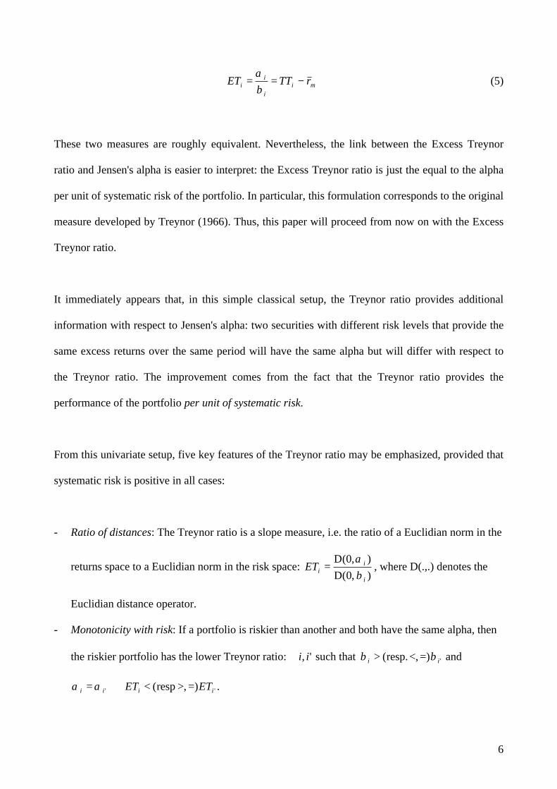
These two measures are roughly equivalent. Nevertheless, the link between the Excess Treynor
ratio and Jensen's alpha is easier to interpret: the Excess Treynor ratio is just the equal to the alpha
per unit of systematic risk of the portfolio. In particular, this formulation corresponds to the original
measure developed by Treynor (1966). Thus, this paper will proceed from now on with the Excess
Treynor ratio.
It immediately appears that, in this simple classical setup, the Treynor ratio provides additional
information with respect to Jensen's alpha: two securities with different risk levels that provide the
same excess returns over the same period will have the same alpha but will differ with respect to
the Treynor ratio. The improvement comes from the fact that the Treynor ratio provides the
performance of the portfolio per unit of systematic risk.
From this univariate setup, five key features of the Treynor ratio may be emphasized, provided that
systematic risk is positive in all cases:
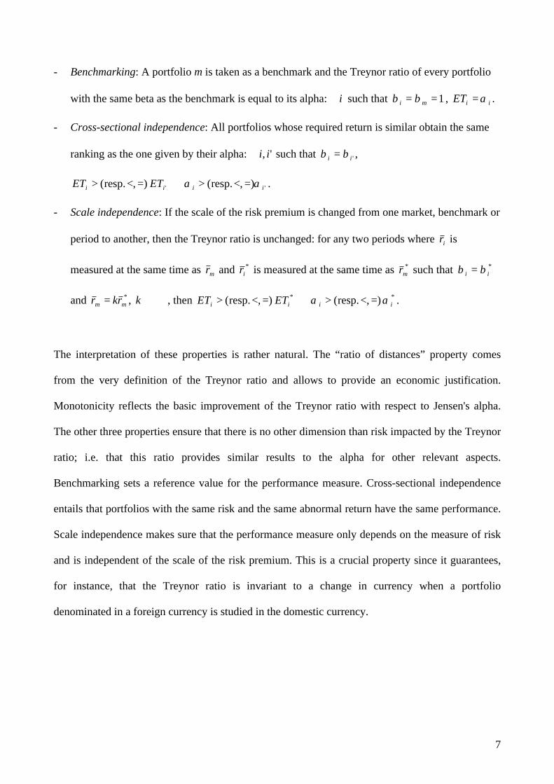
- Ratio of distances: The Treynor ratio is a slope measure, i.e. the ratio of a Euclidian norm in the
returns space to a Euclidian norm in the risk space: ),0(D),0(D
i
iiET
βα
= , where D(.,.) denotes the
Euclidian distance operator.
- Monotonicity with risk: If a portfolio is riskier than another and both have the same alpha, then
the riskier portfolio has the lower Treynor ratio: ', ii∀ such that '), resp.( ii ββ =<> and
'' ), resp( iiii ETET =><⇔= αα .
7
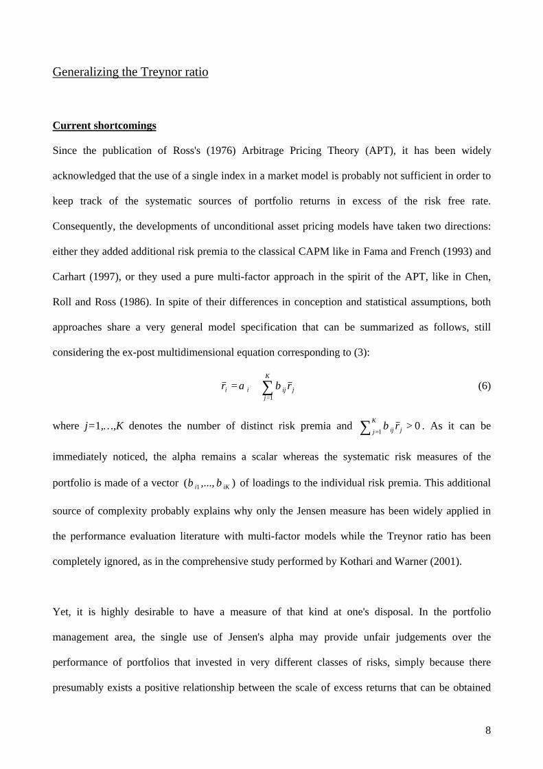
- Benchmarking: A portfolio m is taken as a benchmark and the Treynor ratio of every portfolio
with the same beta as the benchmark is equal to its alpha: i∀ such that 1== mi ββ , iiET α= .
- Cross-sectional independence: All portfolios whose required return is similar obtain the same
ranking as the one given by their alpha: ', ii∀ such that 'ii ββ = ,
'' ), resp.( ), resp.( iiii ETET αα =<>⇔=<> .
- Scale independence: If the scale of the risk premium is changed from one market, benchmark or
period to another, then the Treynor ratio is unchanged: for any two periods where ir is
measured at the same time as mr and *ir is measured at the same time as *
mr such that *ii ββ =
and *mm rkr = , +ℜ∈k , then ** ), resp.( ), resp.( iiii ETET αα =<>⇔=<> .
The interpretation of these properties is rather natural. The “ratio of distances” property comes
from the very definition of the Treynor ratio and allows to provide an economic justification.
Monotonicity reflects the basic improvement of the Treynor ratio with respect to Jensen's alpha.
The other three properties ensure that there is no other dimension than risk impacted by the Treynor
ratio; i.e. that this ratio provides similar results to the alpha for other relevant aspects.
Benchmarking sets a reference value for the performance measure. Cross-sectional independence
entails that portfolios with the same risk and the same abnormal return have the same performance.
Scale independence makes sure that the performance measure only depends on the measure of risk
and is independent of the scale of the risk premium. This is a crucial property since it guarantees,
for instance, that the Treynor ratio is invariant to a change in currency when a portfolio
denominated in a foreign currency is studied in the domestic currency.
8
Generalizing the Treynor ratio
Current shortcomings
Since the publication of Ross's (1976) Arbitrage Pricing Theory (APT), it has been widely
acknowledged that the use of a single index in a market model is probably not sufficient in order to
keep track of the systematic sources of portfolio returns in excess of the risk free rate.
Consequently, the developments of unconditional asset pricing models have taken two directions:
either they added additional risk premia to the classical CAPM like in Fama and French (1993) and
Carhart (1997), or they used a pure multi-factor approach in the spirit of the APT, like in Chen,
Roll and Ross (1986). In spite of their differences in conception and statistical assumptions, both
approaches share a very general model specification that can be summarized as follows, still
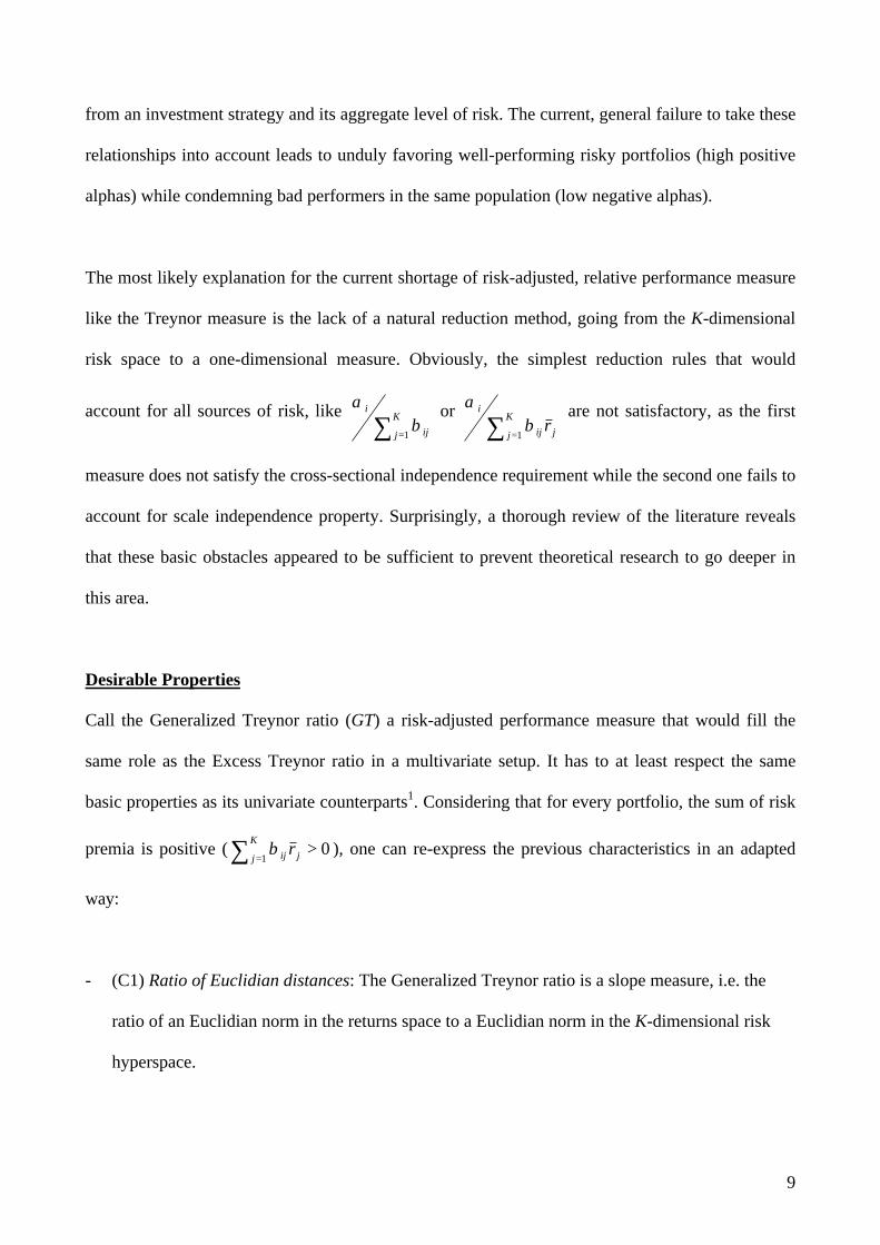
considering the ex-post multidimensional equation corresponding to (3):
∑=
+=K
jjijii rr
1
βα (6)
where j=1,…,K denotes the number of distinct risk premia and 01
>∑ =
K
j jij rβ . As it can be
immediately noticed, the alpha remains a scalar whereas the systematic risk measures of the
portfolio is made of a vector ),...,( 1 iKi ββ of loadings to the individual risk premia. This additional
source of complexity probably explains why only the Jensen measure has been widely applied in
the performance evaluation literature with multi-factor models while the Treynor ratio has been
completely ignored, as in the comprehensive study performed by Kothari and Warner (2001).
Yet, it is highly desirable to have a measure of that kind at one's disposal. In the portfolio
management area, the single use of Jensen's alpha may provide unfair judgements over the
performance of portfolios that invested in very different classes of risks, simply because there
presumably exists a positive relationship between the scale of excess returns that can be obtained
9
from an investment strategy and its aggregate level of risk. The current, general failure to take these
relationships into account leads to unduly favoring well-performing risky portfolios (high positive
alphas) while condemning bad performers in the same population (low negative alphas).
The most likely explanation for the current shortage of risk-adjusted, relative performance measure
like the Treynor measure is the lack of a natural reduction method, going from the K-dimensional
risk space to a one-dimensional measure. Obviously, the simplest reduction rules that would
account for all sources of risk, like ∑ =
K
j ij
i
1β
α or ∑ =
K
j jij
i
r1β
α are not satisfactory, as the first
measure does not satisfy the cross-sectional independence requirement while the second one fails to
account for scale independence property. Surprisingly, a thorough review of the literature reveals
that these basic obstacles appeared to be sufficient to prevent theoretical research to go deeper in
this area.
Desirable Properties
Call the Generalized Treynor ratio (GT) a risk-adjusted performance measure that would fill the
same role as the Excess Treynor ratio in a multivariate setup. It has to at least respect the same
basic properties as its univariate counterparts1. Considering that for every portfolio, the sum of risk
premia is positive ( 01
>∑ =
K
j jij rβ ), one can re-express the previous characteristics in an adapted
way:
- (C1) Ratio of Euclidian distances: The Generalized Treynor ratio is a slope measure, i.e. the
ratio of an Euclidian norm in the returns space to a Euclidian norm in the K-dimensional risk
hyperspace.
10
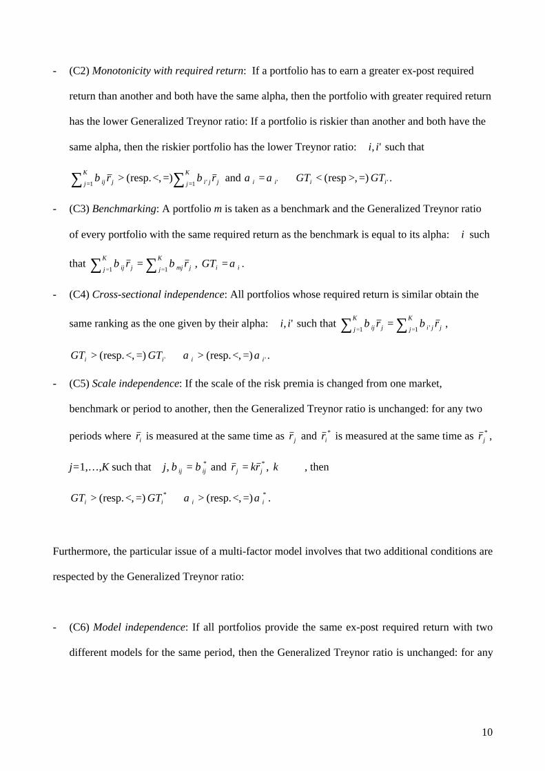
- (C2) Monotonicity with required return: If a portfolio has to earn a greater ex-post required
return than another and both have the same alpha, then the portfolio with greater required return
has the lower Generalized Treynor ratio: If a portfolio is riskier than another and both have the
same alpha, then the riskier portfolio has the lower Treynor ratio: ', ii∀ such that
∑∑ ===<>
K
j jjiK
j jij rr1 '1
), resp.( ββ and '' ), resp( iiii GTGT =><⇔= αα .
- (C3) Benchmarking: A portfolio m is taken as a benchmark and the Generalized Treynor ratio
of every portfolio with the same required return as the benchmark is equal to its alpha: i∀ such
that ∑∑ ===
K
j jmjK
j jij rr11ββ , iiGT α= .
- (C4) Cross-sectional independence: All portfolios whose required return is similar obtain the
same ranking as the one given by their alpha: ', ii∀ such that ∑∑ ===
K
j jjiK
j jij rr1 '1ββ ,
'' ), resp.( ), resp.( iiii GTGT αα =<>⇔=<> .
- (C5) Scale independence: If the scale of the risk premia is changed from one market,
benchmark or period to another, then the Generalized Treynor ratio is unchanged: for any two
periods where ir is measured at the same time as jr and *ir is measured at the same time as *
jr ,
j=1,…,K such that * , ijijj ββ =∀ and *jj rkr = , +ℜ∈k , then
** ), resp.( ), resp.( iiii GTGT αα =<>⇔=<> .
Furthermore, the particular issue of a multi-factor model involves that two additional conditions are
respected by the Generalized Treynor ratio:
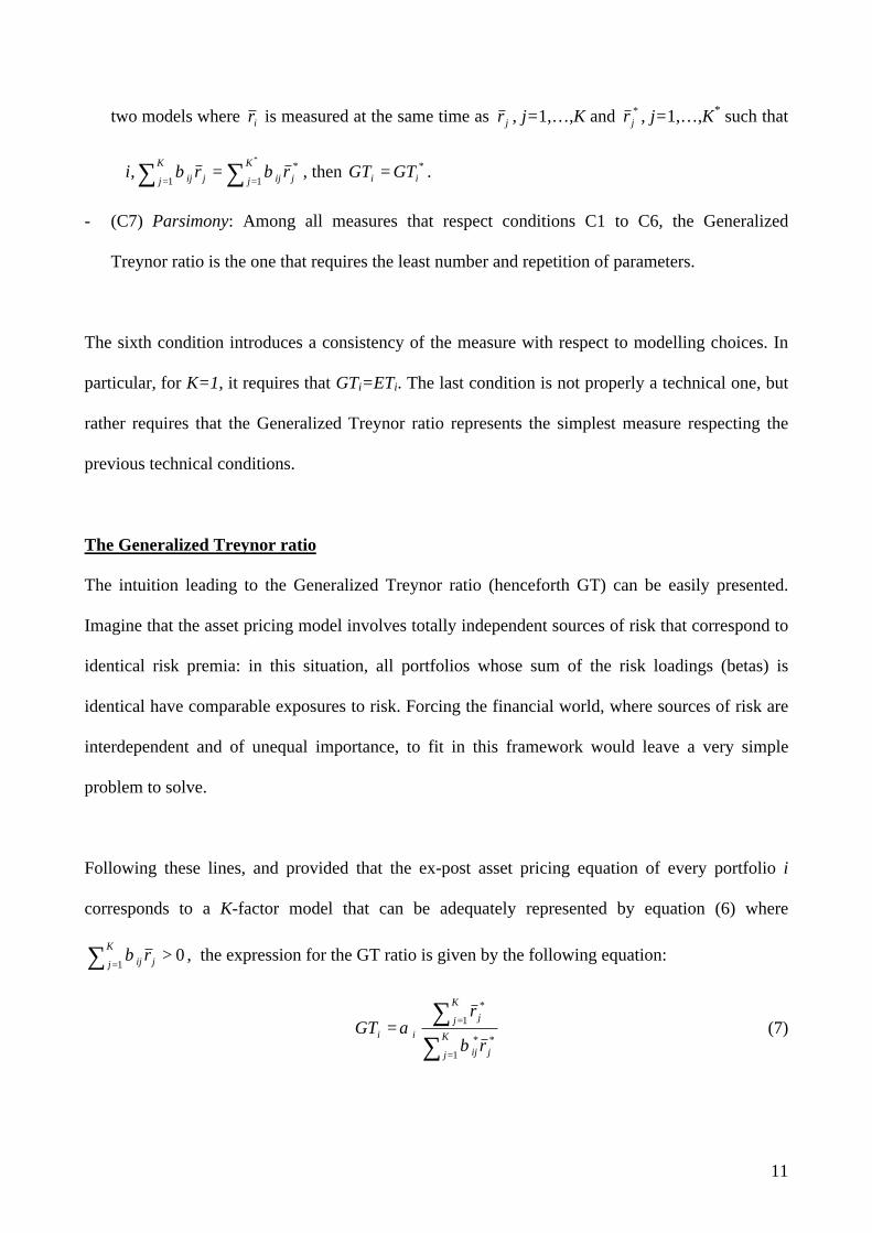
- (C6) Model independence: If all portfolios provide the same ex-post required return with two
different models for the same period, then the Generalized Treynor ratio is unchanged: for any
11
two models where ir is measured at the same time as jr , j=1,…,K and *jr , j=1,…,K* such that
∑∑ ===∀
*
1*
1,
K
j jijK
j jij rri ββ , then * ii GTGT = .
- (C7) Parsimony: Among all measures that respect conditions C1 to C6, the Generalized
Treynor ratio is the one that requires the least number and repetition of parameters.
The sixth condition introduces a consistency of the measure with respect to modelling choices. In
particular, for K=1, it requires that GTi=ETi. The last condition is not properly a technical one, but
rather requires that the Generalized Treynor ratio represents the simplest measure respecting the
previous technical conditions.
The Generalized Treynor ratio
The intuition leading to the Generalized Treynor ratio (henceforth GT) can be easily presented.
Imagine that the asset pricing model involves totally independent sources of risk that correspond to
identical risk premia: in this situation, all portfolios whose sum of the risk loadings (betas) is
identical have comparable exposures to risk. Forcing the financial world, where sources of risk are
interdependent and of unequal importance, to fit in this framework would leave a very simple
problem to solve.
Following these lines, and provided that the ex-post asset pricing equation of every portfolio i
corresponds to a K-factor model that can be adequately represented by equation (6) where
01
>∑ =
K
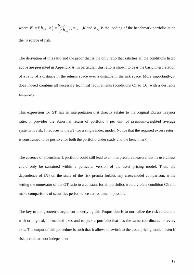
j jij rβ , the expression for the GT ratio is given by the following equation:
∑∑
=
==K
j jij
K
j j
iir
rGT
1**
1*
βα (7)
12
where mjjj rr β=* , mj
ijij β
ββ =* , j=1,…,K and mjβ is the loading of the benchmark portfolio m on
the j's source of risk.
The derivation of this ratio and the proof that is the only ratio that satisfies all the conditions listed
above are presented in Appendix A. In particular, this ratio is shown to bear the basic interpretation
of a ratio of a distance in the returns space over a distance in the risk space. More importantly, it
does indeed combine all necessary technical requirements (conditions C1 to C6) with a desirable
simplicity.
This expression for GTi has an interpretation that directly relates to the original Excess Treynor
ratio: it provides the abnormal return of portfolio i per unit of premium-weighted average
systematic risk. It reduces to the ETi for a single index model. Notice that the required excess return
is constrained to be positive for both the portfolio under study and the benchmark.
The absence of a benchmark portfolio could still lead to an interpretable measure, but its usefulness
could only be sustained within a particular version of the asset pricing model. Then, the
dependence of GTi on the scale of the risk premia forbids any cross-model comparison, while
setting the numerator of the GT ratio to a constant for all portfolios would violate condition C5 and
make comparisons of securities performance across time impossible.
The key to the geometric argument underlying this Proposition is to normalize the risk referential
with orthogonal, normalized axes and to pick a portfolio that has the same coordinates on every
axis. The output of this procedure is such that it allows to switch to the asset pricing model, even if
risk premia are not independent.
13
A crucial property of this ratio is the perfect independence of the measure with the choice of model
specification, provided the compared models are versions of each other, i.e. they provide exactly
the same required returns for all portfolios. This is verified because the numerator and denominator
of the ratio in equation (7) are both independent of the model parameterization provided that it
accounts for the same risk dimensions. A test of equalities of the GT ratio for all portfolios could be
more relevant to test the consistency of different asset pricing models than a direct test on the
Jensen's alphas, obviously less precise.
One may wonder why deriving such a simple formula, and especially why the financial literature
has never emphasized its usefulness. The reason probably lies in fact that such a formula proposed
without proper justification of its applicability would be useless for the financial community. Since
no performance measure is acceptable if it is not accepted by the whole funds industry, its isolate
adoption would just be taken as another episode in the self-promotion of funds managers.
Through its compliance with all listed basic conditions, the GT ratio is justified on geometrical as
well as analytical grounds. The reduction of a multi-dimensional space into one single distance
measure had not yet been performed, probably because it is not natural to consider that portfolios
with very different risk profiles but with the same overall exposure to the sources of risk priced by
the market could share a single unidimensional risk measure. Such a simplification might be
considered as arbitrary, as there are many ways to realize this projection. As a matter of fact, the
GT ratio is not the only measure satisfying all desirable technical conditions, but it is the simplest
and most parsimonious one, which is a valuable asset for practitioners.
An Empirical Example
14
The measure of risk-adjusted performance I propose has been shown to be of theoretical relevance,
i.e. it is the most parsimonious measure that respects a set of conditions that ensures its robustness
to various model, benchmark or scale specifications. This would remain at the stage of a probably
nice but irrelevant exercise if the qualities of the GT ratio could not be demonstrated in practice. In
particular, the very fundamental criticism of the design of this measure, even in the single factor
CAPM setup, is related to the usefulness of designing a performance measure per unit of systematic
risk. The underlying rationale is simple: as it is undoubtedly less intuitive than Jensen's alpha, it
should provide a clearly superior portfolio ranking ability as a compensation; if it fails to do so,
why bother with such a ratio ? Indeed, Jensen's alpha also respects conditions C3 to C6 and is
obviously superior to the Generalized Treynor ratio for condition C7; it only fails to respect
condition C2. This is a very important violation, though, because the availability of a riskless asset
and the use of homemade leverage (as illustrated in the classical textbook-example of lending and
borrowing that enables the investor to choose any location along the Capital Market Line) proves
the unequivocal superiority of the Treynor Ratio – and so of its generalized version – over the
alpha. But this remains a theoretical advantage; if portfolio rankings are barely different for both
ratios, then the simplicity of Jensen's alpha is practically superior.
The empirical illustration that I present in this paper is meant to address this criticism with the use
of real data. This brings a major difference with respect to the conceptual framework presented
above: for a given portfolio, a change in the benchmark, in the model specification or in the period
will almost automatically change its statistical levels of required returns and of excess return.
Therefore, it is highly likely that any such change will induce variations in performance measures
for all portfolios, and so changes in rankings. The goal of this section is therefore to assess whether
the claimed robustness of the GT ratio with respect to changes in benchmarks, that accounts for the
15
change in the alpha but also in the portfolio's and the benchmark's required returns, leaves of more
reliable picture of the performance rankings of mutual funds than if the alpha is used as an
alternative.
I use a sample of nine mutual funds, each of them being in the top ten performing fund, in absolute
terms, of their category over either a one-year or a five-year period ending April 1, 2003, with an
additional requirement that all funds should have a nine-year history of returns. Categories have
been defined as the classical Large/Midcap/Small and Growth/Blend/Value styles. Data has been
extracted from Yahoo! Finance.
The asset pricing model of reference is the four-factor specification put forward by Carhart (1997).
Monthly returns for the size (SMB), book-to-market (HML) and momentum (PR1YR) factors has
been extracted from Eugene Fama's website.The tested variations of this model are the Fama and
French (1993) 3-factor model and the single index CAPM. The same underlying risk premia are
used throughout.
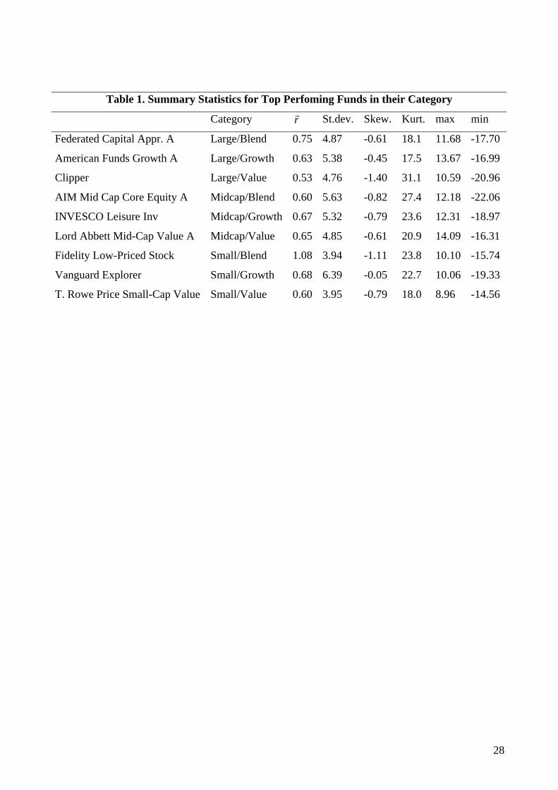
Insert Table 1 approximately here
Table 1 provides summary statistics of returns for these funds in excess of the three-months T-Bill
rate and adjusted for dividends over the January 94-December 2002 period. They all exhibit a total
rate of return ranging from 0.53% to 1.08%, corresponding to an equivalent yearly premium of
6.5% to 13.8%. Standard deviations and ranges of variation are fairly similar from one fund to
another. Their negative skewness and very high kurtosis suggest that their returns are highly
nonnormal2, with fat tails and negative asymmetry. Therefore, the use of a single index model, like
the CAPM, is not justified on distributional grounds.
16
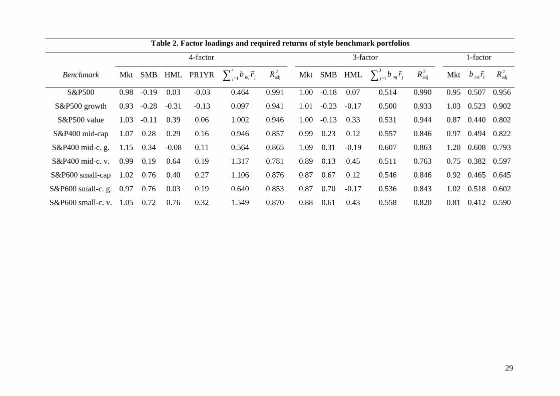
Insert Table 2 approximately here
Nine indices computed by Standard & Poors, each one corresponding to the underlying style of the
funds, are used as benchmarks. Table 2 reports the risk sensitivities and required returns of these
benchmarks for each asset pricing model. Not surprisingly, the momentum factor dramatically
alters the total risk premia.\ For the single model they range between 0.38% and 0.61%. The range
is narrowed to an interval of less than 11 b.p. (0.607%-0.500%) for the three-factor model, while it
explodes to more than 150 b.p. (1.549%-0.097%) when momentum is included. This shows the
extreme sensitivity of empirical results to the choice of asset pricing models. Such a finding
somehow contradicts, one the one hand, the hypothesis of equivalent asset pricing models
underlying the GT ratio; on the other hand, it clearly emphasizes the need for a performance ratio
that yields consistent rankings across asset pricing model specifications, and so provides a practical
justification to this empirical exercise.
The Fama-French specification significantly outperforms the one-factor CAPM, but the adjusted R2
for the four-factor regressions are slightly better. Thus, although the risk premia of the benchmarks
are more volatile with the latter model, I use it as the base case to assess the robustness of portfolio
performance measures with respect to changes in benchmark portfolios and in asset pricing models.
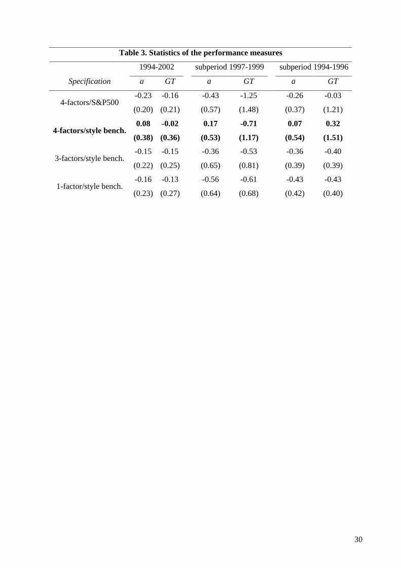
Insert Table 3 approximately here
The mean and standard deviations (between parentheses) of Jensen's alpha and of the Generalized
Treynor ratios for each asset pricing model are displayed in Table 3. To ensure that they correctly
capture the relative performance of the funds, the alphas of their respective benchmarks have been
17
substracted from their absolute value. For the four-factor specification, the Table reports
performance measures computed against style benchmarks as well as against the single S&P500
portfolio. The test has been performed for the whole 9-year period and for the 1994-1996 and 1997-
1999 subperiods. The 2000-2002 period could not be tested as the risk premia for all benchmark
portfolios were negative, making it impossible to compute economically significant performance
measures. Results suggest that the mean Generalized Treynor ratio is more consistently negative
that the alphas.3 At the same time, their dispersion is much greater, as indicated by higher standard
deviations than for the alphas. Not surprisingly, by accounting for the risk exposures of each
portfolio, the range of observed values of the GT ratios is much broader than the one of alphas,
indicating a superior ability to discriminate funds on a cardinal basis.
This dispersion can be a double-edged weapon if the values provided by the GT ratio are less
reliable than the classically used Jensen's alpha. It is therefore necessary to assess the robustness of
the competing performance measures for the nine selected funds, by checking their sensitivity to
changes in referential.
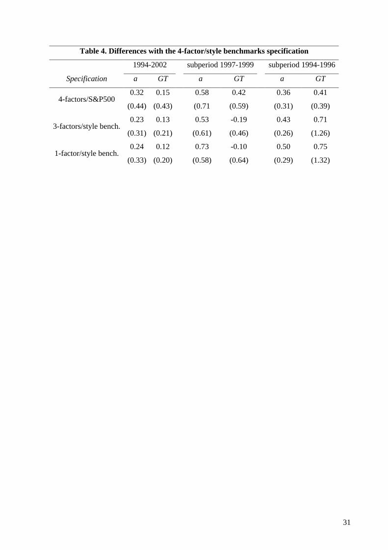
Insert Table 4 approximately here
Table 4 reports the mean and standard deviations of the differences between the values of the
alphas and of the Generalized Treynor Ratios under the base case and the alternative specifications.
For the whole nine-year period, results are strikingly in favor of the GT ratio. The mean difference
between values of this measure under the four-factor model with style benchmarks is
approximately half the one of the alphas, for every alternative specification. The lower standard
deviation of these differences also suggests that alphas are less stable from one model or
benchmark to another.
18
For the subperiods, the picture is different. The Generalized Treynor ratio still proves its superiority
over the alpha in the 1997-1999 period, with lower average differences and similar standard
deviations, but seems to perform poorly in the 1994-1996 period. The presence of a large outlier for
the GT of one mutual fund mostly explains this behavior.
Put altogether, this limited piece of parametric evidence indicates that the new performance
measure proposed in this article exhibits many desirable properties, as it provides a greater
dispersion among mutual funds than Jensen's alpha does but, at the same time, remains more robust
for a change in the model or the benchmark chosen. This superior performance looks very
convincing for a long horizon, but is more disputable over shorter time periods. Since this seems to
be mainly due to the presence of very large values of this ratio – remember that the GT ratio uses
the total required return of the portfolio in the numerator; if it is close to zero, the ratio is likely to
explode –, some nonparametric measures of reliability may provide a better picture of the
robustness of the performance measures under study.
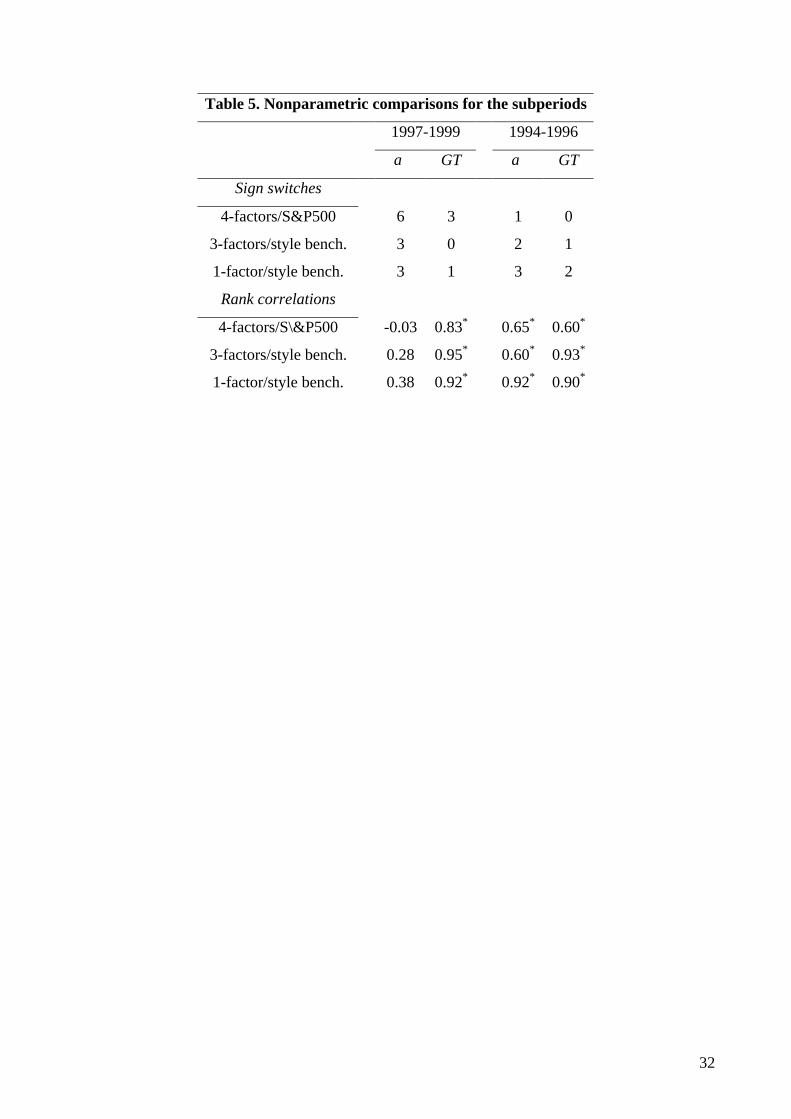
Insert Table 5 approximately here
Some insights regarding these matters are provided in Table 5. The relative performance of the
measures are examined for the two subperiods. The first indicator is the number of sign switches
for the nine mutual funds, i.e. the number of times a performance measure is positive (resp.
negative) for the base case and negative when the benchmark of the asset pricing model is
modified. The second indicator is Spearman's rank correlation coefficient between rankings made
under the alternative specifications. The asterisk means that the absence of correlation can be
rejected at the 5% level. Results confirm the hypothesis previously put forward: the GT Ratio
19
generates more extreme values, but appears to be superior to the alpha when the signs and rankings
are considered. Sign violations are consistently less numerous for the GT ratio, indicating that
positive or negative abnormal performances are more reliable when using this measure. On the
other hand, the ordering of funds remains more stable with this new measure, which contributes to
the making of rankings fairly independent of the model or the benchmark used.
Conclusion
This article proposed to generalize the Treynor ratio in a multi-index setup through the recourse to
a geometric argument: since the original measure represents a proportion of distances in the returns
and in the systematic risk referentials, a multi-dimensional counterpart can be justified in an
orthonormal risk referential. From that starting point, the proposed Generalized Treynor ratio
represents the simplest measure that bears this interpretation and, at the same time, manages to
conserve the key properties of its one-dimensional counterpart. For a given portfolio, its formula
simplifies to a simple ratio of Jensen's alpha over an average of the betas.
The empirical comparison of the Generalized Treynor ratio with Jensen's alpha, although very
preliminary, provides a promising set of results concerning the robustness of this new performance
measure. It appears to bear quite remarkably changes in asset pricing specification or in
benchmarks. This illustration is not meant to be exhaustive, but simply to justify the use of this
ratio as a credible alternative to Jensen's alpha, for instance for portfolio rankings or simple to
check the ability for a manager to obtain positive abnormal performance. It is naturally important to
assess whether the long-lasting debates over performance persistence of mutual funds or of relative
performance of hedge funds would benefit from the availability of this refined measure.
20
Unlike many academic articles, this paper has no ambition to be technically involved, but simply
aims at filling a strange gap in the performance evaluation literature. The lack of risk-normalized
performance measure for multi-factor models had increasingly become a painful anomaly in the
current blossoming of empirical studies focusing on mutual and hedge funds performance. By
allowing a safe comparability of performances across risk exposures but also across models and
units, the simple formula for the Generalized Treynor ratio has the potential to create more
objective classification procedures. The simple design of this measure, instead of being a hindrance
for its adoption, could be the best guarantee of a wide use in the financial communities, whether
academic or professional. It is up to them to decide.
21
References
Carhart, Mark M. 1997. “On persistence in mutual funds performance.” Journal of Finance, vol.
52, no. 1 (March): 57-82.
Chen, Nai-Fu, Richard Roll and Stephen A. Ross. 1986. “Economic forces and the stock market.”
Journal of Business, vol. 59, no. 3 (July): 383-403.
Connor, Gregory and Robert A. Korajczyk. 1986. “Performance measurement with the arbitrage
pricing theory. A new framework for analysis.” Journal of Financial Economics, vol. 15, 373-394.
Fama, Eugene F. 1972. “Components of investment performance.” Journal of Finance, vol. 27, no.
3 (June): 551-567.
Fama, Eugene. F. and Kenneth French. 1993. “Common risk factors in the returns of stocks and
bonds.” Journal of Financial Economics, vol. 33, no. 1 (February): 3-56.
Henriksson, Roy D. and Robert C. Merton. 1981. “On market timing and investment performance.
II. Statistical procedures for evaluating forecasting skills.” Journal of Business, vol. 54, no. 4
(October): 513-533.
Jensen, Michael J. 1968. “The Performance of Mutual Funds in the Period 1945-1964.” Journal of
Finance, vol. 23, no. 2 (May): 389-416.
Kothari, S.P. and Jerold B. Warner. 2001. “Evaluating mutual fund performance.” Journal of
Finance, vol. 56, no. 5 (October): 1985-2010.
Lintner, John. 1965. “The valuation of risk assets and the selection of risky investments in stock
portfolios and capital budgets.” Review of Economics and Statistics, vol 47, no. 1 (February): 13-
37.
Modigliani, Franco and Leah Modigliani. 1997. “Risk-adjusted performance.” Journal of Portfolio
Management, vol. 23, no. 2 (Winter): 45-54.
22
Mossin, Jan. 1966. “Equilibrium in capital asset market.” Econometrica, vol 34 (October): 768-
783.
Ross, Stephen A. 1976. “The arbitrage theory of capital asset pricing.” Journal of Economic
Theory, vol 13, no. 3 (December): 341-360.
Sharpe, William F. 1964. “Capital asset prices: A theory for market equilibrium under conditions of
risk.” Journal of Finance, vol 19, no. 3 (September): 425-442.
Sharpe, William F. 1966. “Mutual fund performance.” Journal of Business, vol 39, no. 1 (January):
119-138.
Sharpe, William F. 1992. “Asset allocation: Management style and performance measurement.”
Journal of Portfolio Management, vol. 18, no. 2 (Winter): 29-34.
Sharpe, William F. 1994. “The Sharpe ratio.” Journal of Portfolio Management, vol. 21, no.1
(Fall): 49-58.
Treynor, Jack L. 1961. “Toward a Theory of Market Value of Risky Assets.” Mimeo, subsequently
published in Korajczyk, Robert A. (1999), Asset Pricing and Portfolios Performance: Models,
Strategy and Performance Metrics. London: Risk Books.
Treynor, Jack L. 1966. “How to rate management investment funds.” Harvard Business Review,
vol 43, no. 1 (January-February): 63-75.
Treynor, Jack L., and Fisher Black. 1973. “How to use security analysis to improve portfolio
selection.” Journal of Business, vol 46, no. 1 (January): 66-86.
Treynor, Jack L. and Kay Mazuy. 1966. “Can mutual funds outguess the market ?” Harvard
Business Review, vol 44, no. 4 (July-August): 131-136.
23
Notes
1 It is worth mentioning that this section is not meant to propose an axiomatic approach of what
should be a measure of risk-adjusted portfolio performance, but rather to represent the key features
of the Treynor ratio in a multivariate setup.
2 This is supported by the Jarque-Bera statistics, available upon request.
3 The noticeable exception of the positive average Generalized Treynor ratio for the 4-factor, style
benchmark specification in the 1994-1996 subperiod is due to a portfolio with a very high loading
on the momentum factor that has a GT higher than 4.
24
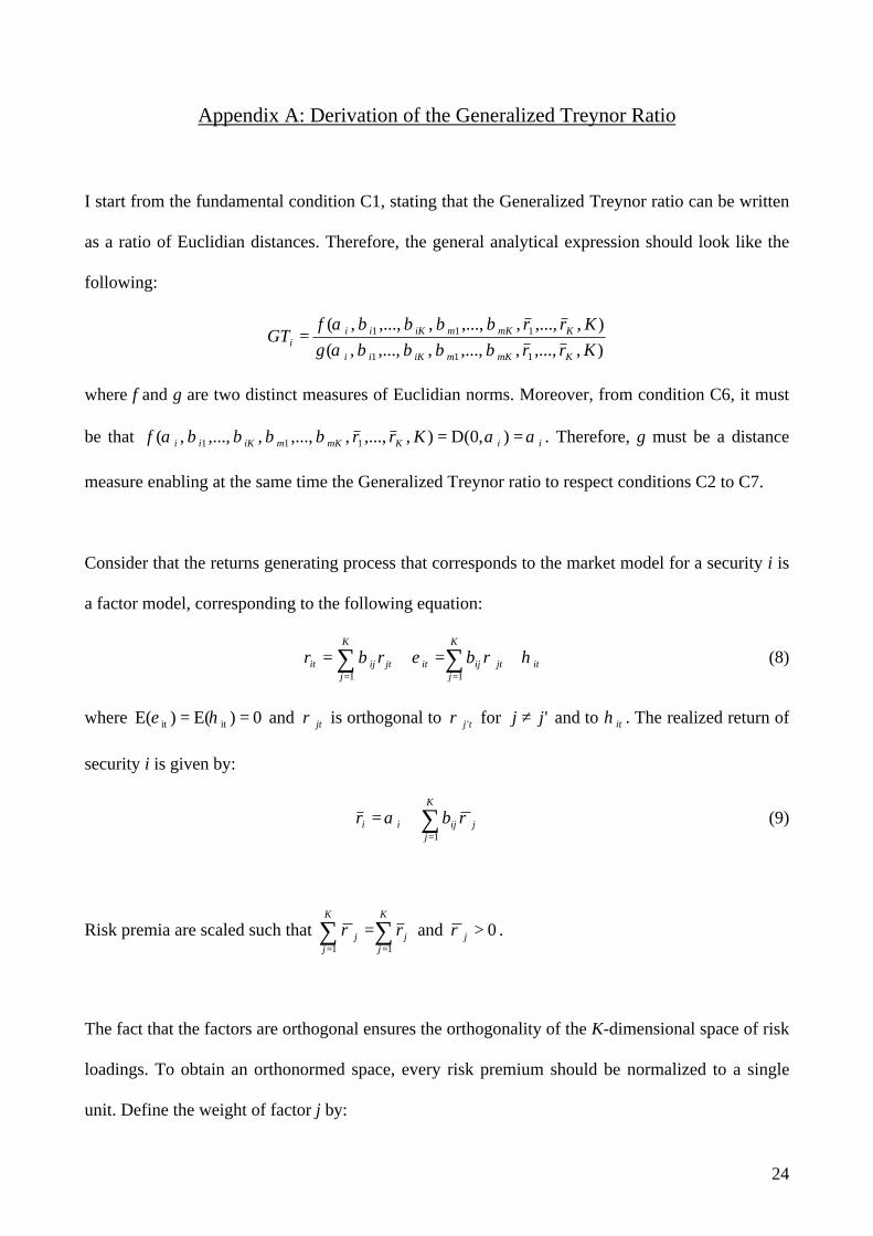
Appendix A: Derivation of the Generalized Treynor Ratio
I start from the fundamental condition C1, stating that the Generalized Treynor ratio can be written
as a ratio of Euclidian distances. Therefore, the general analytical expression should look like the
following:
),,...,,,...,,,...,,(),,...,,,...,,,...,,(
111
111
KrrgKrrf
GTKmKmiKii
KmKmiKiii ββββα
ββββα=
where f and g are two distinct measures of Euclidian norms. Moreover, from condition C6, it must
be that iiKmKmiKii Krrf ααββββα == ),0(D),,...,,,...,,,...,,( 111 . Therefore, g must be a distance
measure enabling at the same time the Generalized Treynor ratio to respect conditions C2 to C7.
Consider that the returns generating process that corresponds to the market model for a security i is
a factor model, corresponding to the following equation:
∑∑==
+=+=K
jitjtij
K
jitjtijit brr
11
ηρεβ (8)
where 0)E()E( itit == ηε and jtρ is orthogonal to tj 'ρ for 'jj ≠ and to itη . The realized return of
security i is given by:
∑=
+=K
jjijii br
1
ρα (9)
Risk premia are scaled such that ∑∑==
=K
jj
K
jj r
11
ρ and 0>jρ .
The fact that the factors are orthogonal ensures the orthogonality of the K-dimensional space of risk
loadings. To obtain an orthonormed space, every risk premium should be normalized to a single
unit. Define the weight of factor j by:
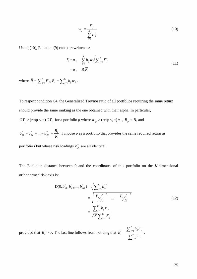
25
∑=
=K
jj
jjw
1
ρ
ρ(10)
Using (10), Equation (9) can be rewritten as:
( )RB
wbr
ii
K
j
K
j jjijii
+=
+= ∑ ∑=
=
α
ρα1
1 (11)
where ∑∑ ====
K
j jijiK
j j wbBR11
,ρ .
To respect condition C4, the Generalized Treynor ratio of all portfolios requiring the same return
should provide the same ranking as the one obtained with their alpha. In particular,
pi GTGT ), resp( =<> for a portfolio p where ip αα ), resp( =<> , ip BB = and
KB
bbb ipKpp ==== **
2*
1 ... . I choose p as a portfolio that provides the same required return as
portfolio i but whose risk loadings *pjb are all identical.
The Euclidian distance between 0 and the coordinates of this portfolio on the K-dimensional
orthonormed risk axis is:
∑∑
∑
=
=
=
=
++
=
=
K
j j
K
j jij
ii
K
j pjpKpp
K
b
KB
KB
bbbb
1
1
22
12***
2*
1
...
),...,,D(0,
ρ
ρ
(12)
provided that 0>iB . The last line follows from noticing that ∑
∑=
==K
j j
K
j jij
i
bB
1
1
ρ
ρ.
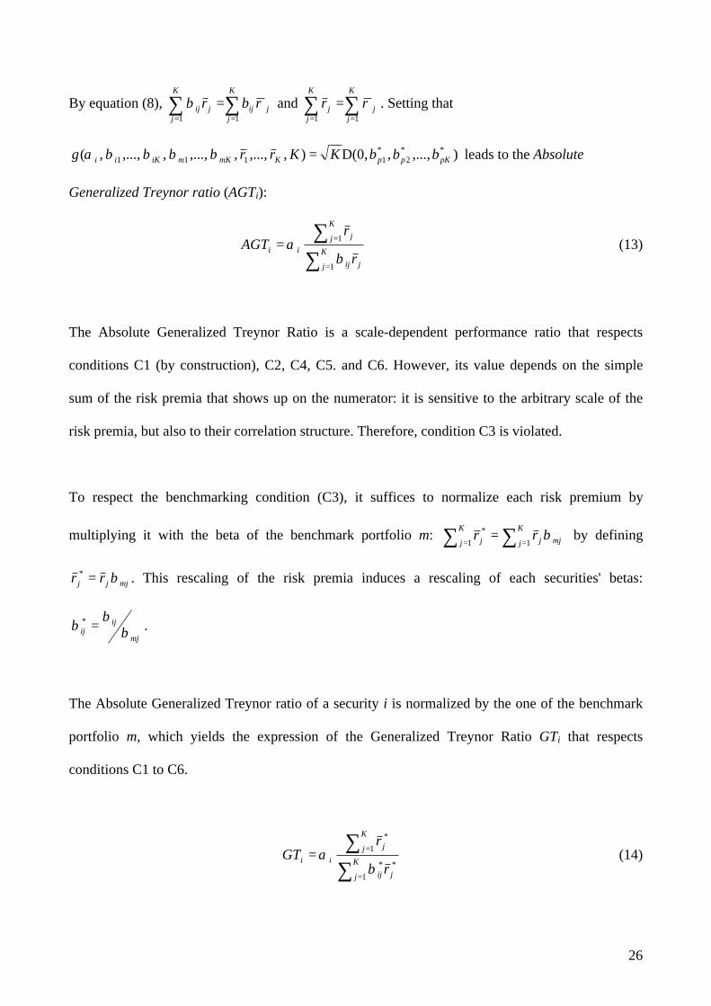
26
By equation (8), ∑∑==
=K
jjij
K
jjij br
11
ρβ and ∑∑==
=K
jj
K
jjr
11
ρ . Setting that
),...,,D(0,),,...,,,...,,,...,,( **2
*1111 pKppKmKmiKii bbbKKrrg =ββββα leads to the Absolute
Generalized Treynor ratio (AGTi):
∑∑
=
==K
j jij
K
j j
iir
rAGT
1
1
βα (13)
The Absolute Generalized Treynor Ratio is a scale-dependent performance ratio that respects
conditions C1 (by construction), C2, C4, C5. and C6. However, its value depends on the simple
sum of the risk premia that shows up on the numerator: it is sensitive to the arbitrary scale of the
risk premia, but also to their correlation structure. Therefore, condition C3 is violated.
To respect the benchmarking condition (C3), it suffices to normalize each risk premium by
multiplying it with the beta of the benchmark portfolio m: ∑∑ ===
K
j mjjK
j j rr11
* β by defining
mjjj rr β=* . This rescaling of the risk premia induces a rescaling of each securities' betas:
mj
ijij β
ββ =* .
The Absolute Generalized Treynor ratio of a security i is normalized by the one of the benchmark
portfolio m, which yields the expression of the Generalized Treynor Ratio GTi that respects
conditions C1 to C6.
∑∑
=
==K
j jij
K
j j
iir
rGT
1**
1*
βα (14)
27
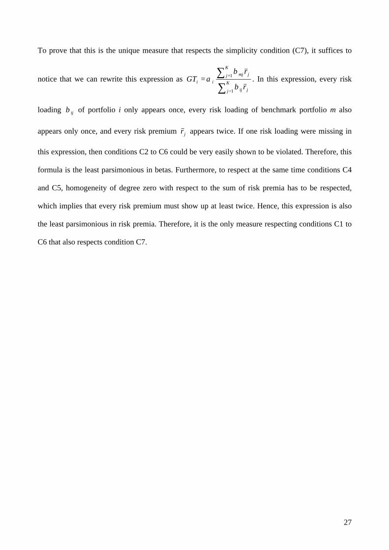
To prove that this is the unique measure that respects the simplicity condition (C7), it suffices to
notice that we can rewrite this expression as ∑∑
=
==K
j jij
K
j jmj
iir
rGT
1
1
β
βα . In this expression, every risk
loading ijβ of portfolio i only appears once, every risk loading of benchmark portfolio m also
appears only once, and every risk premium jr appears twice. If one risk loading were missing in
this expression, then conditions C2 to C6 could be very easily shown to be violated. Therefore, this
formula is the least parsimonious in betas. Furthermore, to respect at the same time conditions C4
and C5, homogeneity of degree zero with respect to the sum of risk premia has to be respected,
which implies that every risk premium must show up at least twice. Hence, this expression is also
the least parsimonious in risk premia. Therefore, it is the only measure respecting conditions C1 to
C6 that also respects condition C7.
28
Table 1. Summary Statistics for Top Perfoming Funds in their Category
Category r St.dev. Skew. Kurt. max min
Federated Capital Appr. A Large/Blend 0.75 4.87 -0.61 18.1 11.68 -17.70
American Funds Growth A Large/Growth 0.63 5.38 -0.45 17.5 13.67 -16.99
Clipper Large/Value 0.53 4.76 -1.40 31.1 10.59 -20.96
AIM Mid Cap Core Equity A Midcap/Blend 0.60 5.63 -0.82 27.4 12.18 -22.06
INVESCO Leisure Inv Midcap/Growth 0.67 5.32 -0.79 23.6 12.31 -18.97
Lord Abbett Mid-Cap Value A Midcap/Value 0.65 4.85 -0.61 20.9 14.09 -16.31
Fidelity Low-Priced Stock Small/Blend 1.08 3.94 -1.11 23.8 10.10 -15.74
Vanguard Explorer Small/Growth 0.68 6.39 -0.05 22.7 10.06 -19.33
T. Rowe Price Small-Cap Value Small/Value 0.60 3.95 -0.79 18.0 8.96 -14.56
29
Table 2. Factor loadings and required returns of style benchmark portfolios
4-factor 3-factor 1-factor
Benchmark Mkt SMB HML PR1YR ∑ =
4
1j jmj rβ 2adjR Mkt SMB HML ∑ =
3
1j jmj rβ 2adjR Mkt 11rmβ 2
adjR
S&P500 0.98 -0.19 0.03 -0.03 0.464 0.991 1.00 -0.18 0.07 0.514 0.990 0.95 0.507 0.956
S&P500 growth 0.93 -0.28 -0.31 -0.13 0.097 0.941 1.01 -0.23 -0.17 0.500 0.933 1.03 0.523 0.902
S&P500 value 1.03 -0.11 0.39 0.06 1.002 0.946 1.00 -0.13 0.33 0.531 0.944 0.87 0.440 0.802
S&P400 mid-cap 1.07 0.28 0.29 0.16 0.946 0.857 0.99 0.23 0.12 0.557 0.846 0.97 0.494 0.822
S&P400 mid-c. g. 1.15 0.34 -0.08 0.11 0.564 0.865 1.09 0.31 -0.19 0.607 0.863 1.20 0.608 0.793
S&P400 mid-c. v. 0.99 0.19 0.64 0.19 1.317 0.781 0.89 0.13 0.45 0.511 0.763 0.75 0.382 0.597
S&P600 small-cap 1.02 0.76 0.40 0.27 1.106 0.876 0.87 0.67 0.12 0.546 0.846 0.92 0.465 0.645
S&P600 small-c. g. 0.97 0.76 0.03 0.19 0.640 0.853 0.87 0.70 -0.17 0.536 0.843 1.02 0.518 0.602
S&P600 small-c. v. 1.05 0.72 0.76 0.32 1.549 0.870 0.88 0.61 0.43 0.558 0.820 0.81 0.412 0.590
30
Table 3. Statistics of the performance measures
1994-2002 subperiod 1997-1999 subperiod 1994-1996
Specification α GT α GT α GT
4-factors/S&P500-0.23
(0.20)
-0.16
(0.21)
-0.43
(0.57)
-1.25
(1.48)
-0.26
(0.37)
-0.03
(1.21)
4-factors/style bench.0.08
(0.38)
-0.02
(0.36)
0.17
(0.53)
-0.71
(1.17)
0.07
(0.54)
0.32
(1.51)
3-factors/style bench.-0.15
(0.22)
-0.15
(0.25)
-0.36
(0.65)
-0.53
(0.81)
-0.36
(0.39)
-0.40
(0.39)
1-factor/style bench.-0.16
(0.23)
-0.13
(0.27)
-0.56
(0.64)
-0.61
(0.68)
-0.43
(0.42)
-0.43
(0.40)
31
Table 4. Differences with the 4-factor/style benchmarks specification
1994-2002 subperiod 1997-1999 subperiod 1994-1996
Specification α GT α GT α GT
4-factors/S&P5000.32
(0.44)
0.15
(0.43)
0.58
(0.71
0.42
(0.59)
0.36
(0.31)
0.41
(0.39)
3-factors/style bench.0.23
(0.31)
0.13
(0.21)
0.53
(0.61)
-0.19
(0.46)
0.43
(0.26)
0.71
(1.26)
1-factor/style bench.0.24
(0.33)
0.12
(0.20)
0.73
(0.58)
-0.10
(0.64)
0.50
(0.29)
0.75
(1.32)
32
Table 5. Nonparametric comparisons for the subperiods
1997-1999 1994-1996
α GT α GT
Sign switches
4-factors/S&P500 6 3 1 0
3-factors/style bench. 3 0 2 1
1-factor/style bench. 3 1 3 2
Rank correlations
4-factors/S\&P500 -0.03 0.83* 0.65* 0.60*
3-factors/style bench. 0.28 0.95* 0.60* 0.93*
1-factor/style bench. 0.38 0.92* 0.92* 0.90*