Embed Size (px)
Citation preview


1
The gender gap in mathematics achievement:
Evidence from Italian data.
Dalit Contini1, Maria Laura Di Tommaso
2, Silvia Mendolia
3,
Abstract
Gender differences in the STEM (Science Technology Engineering and Mathematics) disciplines
are widespread in most OECD countries and mathematics is the only subject where typically girls
tend to underperform with respect to boys. This paper describes the gender gap in math test scores
in Italy, which is one of the countries displaying the largest differential between boys and girls
according to the Programme for International Student Assessment (PISA). We use data from an
Italian national level learning assessment, involving children in selected grades from second to
tenth. We first analyse the magnitude of the gender gap using OLS regression and school fixed-
effect models for each grade separately. Our results show that girls systematically underperform
boys, even after controlling for an array of individual and family background characteristics, and
that the average gap increases with children‟s age. We then study the gender gap throughout the test
scores distribution, using quantile regression and metric-free methods, and find that the differential
is small at the lowest percentiles of the grade distribution, but large among top performing children.
Finally, we estimate dynamic models relating math performance at two consecutive assessments.
Lacking longitudinal data, we use a pseudo panel technique and find that girls‟ average test scores
are consistently lower than those of boys at all school years, even conditional on previous scores.
JEL: J16; I24; C31.
Keywords Math gender gap, education, school achievement, inequalities, cross-sectional
data, pseudo panel estimation, quantile regression
1 Dept of Economics and Statistics Cognetti de Martiis, Lungo Dora Siena 100, Torino, Italy. [email protected] 2 Dept of Economics and Statistics Cognetti de Martiis, Lungo Dora Siena 100, Torino, Italy.
[email protected] and Collegio Carlo Alberto, Moncalieri, Italy. 3 School of Accounting, Economics, and Finance, University of Wollongong, Northfields Avenue, North Wollongong,
NSW 2522. [email protected]
2
1. Introduction
The traditional gender gap in educational outcomes advantaging boys has been completely filled up
in most industrialized countries, and has now reversed in favour of girls. Girls tend to do better than
boys in reading test scores, in grades completion and repetition at school, in the propensity to
choose academic educational programs in upper secondary school, in tertiary education attendance
and graduation rates. In this perspective, there is now an extensive literature addressing the
underperformance of boys (Department for Education and Skills 2007; Legewie and Di Prete 2012).
However, boys keep doing better than girls in math tests. According to the last available PISA
(Programme for International Students Assessment) data set, Italy is one of the countries with the
highest gender gap in mathematics for 15 years-old students. While the Italian mean test scores in
mathematics are similar to the OECD average, the gender differences in mathematics are much
higher in Italy than the OECD average (a 20 points difference in Italy against an average difference
of 9 points in the OECD). This difference is the second highest among OECD countries with only
Austria displaying a larger difference (OECD 2016). In addition, TIMMS 2015 (Trends in
International Mathematics and Science Study) shows that Italy has the highest gender gap in
mathematics for children in fourth grade among all the 57 countries included in the survey (Mullis
et al 2016). The presence of a substantial females‟ disadvantage in math is of particular importance,
because it is likely to be a cause of the critically low share of women choosing STEM (Science
Technology Engineering and Mathematics) disciplines at university, of gender segregation in the
labour market, and gender pay gaps (European Commission 2006, 2012, 2015; National Academy
of Science, 2007).
Several explanations have been proposed for the existence of the gender gap in mathematics. Some
scholars refer to biological factors (Baron-Cohen and Wheelwright 2004, Baron Cohen et al 2001).
However, as shown by international assessments (OECD 2016, Mullis et al, 2016) the gender gap in
math differs substantially across countries and some contributions (Guiso et al., 2008, De San
Roman and De La Rica, 2012; OECD 2015) provide evidence that the gender gap in math in the
PISA survey is negatively related to country level indexes of gender equality. The literature also
emphasizes the importance of parents and teachers‟ beliefs about boys and girls capacities (Fryer
and Levitt, 2010; Cornwell and Mustard, 2013; Robinson et al., 2014; Jacobs and Bleeker 2004;
Bhanot and Jovanovic 2009). Girls display less math self-efficacy (self-confidence in solving math
related problems) and math self-concept (beliefs in their own abilities), and more anxiety and stress
in doing math related activities (OECD 2015, Heckman and Kautz 2012, 2014; Lubienski et al
2013, Twenge and Campbell 2001). As demonstrated by the recent work by Heckman and

3
colleagues (e.g. Heckman and Kautz 2012, 2014; Heckman and Mosso, 2014), non-cognitive
abilities including motivation and self-esteem are important predictors of success in life and in the
labour market. There is also empirical evidence that girls with mothers working in math-related
occupations lag behind boys as much as those whose mothers are not in math-related occupations
(Fryer and Levitt, 2010; OECD 2015). Schools and educational methods and practices also seem to
matter. Problem solving, class-discussions and investigative work and cognitive activation
strategies have been found to improve girls‟ performances (Boaler 2002; Zohar and Sela 2003;
OECD 2015). In addition, Boaler et al. (2011) and Good, Woodzicka, and Wingfield (2010) show
that girls‟ proficiency increases by using counter-stereotypic pictures with female scientists.
From a policy perspective, it is important to describe when the gap first shows up. Tackling the
gender gap in mathematics at an early stage is more cost-efficient and it can re-address the
inequality when it is still at the beginning before girls choose high schools or university degrees.
Research about the evolution of the gender gap in mathematics from an early age is mainly based
on the US dataset “Early Childhood Longitudinal Study, Kindergarten Class of 1998– 1999”
(ECLS-K) following students from kindergarten through eighth grade. The main finding from these
data is that the math gender gap starts as early as in kindergarten and increases with the age of the
child (Robinson and Lubiensky, 2011; Fryer and Levitt, 2010; Penner and Paret, 2008). Another
relevant result is that the math gender gap is higher for top performing students. Initially boys
appear to do better than girls among well performers and worse at the bottom of the distribution;
however, by third grade, the gender gap, while still larger at the top, appears throughout the
distribution. Moreover, the male advantage among high performers is largest among families with
high parental education. Girls appear to lose ground in math over time in every family structure,
ethnic group, and level of the socio-economic distribution (Fryer and Levitt, 2010).
Differently from the US, in Europe there are not many studies about the evolution of the gender gap
in mathematics during childhood. Cross sectional data sets show that the gender gap in mathematics
exists in 4° and 8° grade (in TIMMS data4) and in 10° grade (in PISA data, OECD 2016) in many
European countries but not much has been done to study its evolution from an early stage. One
obvious reason is the lack of longitudinal data, but even where these data exists, not much research
has been done. Longitudinal studies in UK (LSYPE and the Millennium Cohort Study) report
limited evidence of a substantial gender gap in math (Department for Education and Skills 2007), and
the National Education Panel Study (NEPS) in Germany does not focus on gender inequalities
4 For a detailed description of the gender gap in Math and Science across OECD countries in TIMMS data, see Bedard and Cho (2010).

4
(Blossfeld et al. 2011). However, according to the PISA assessment (OECD, 2016), both countries
display a significant math gender gap in favour of boys at age 15.
This lack of attention to the study of the evolution of the gender gap in mathematics in European
countries is also mirrored by a lack of policies to re-address it at an early age. Many policies and
campaigns have focused on high school students, women and STEM subjects at university, or on
gender inequality in research and innovation5 but there has been a lack of policies at the lower
levels of the educational systems.
As for Italy, there are currently no systematic contributions on the evolution of the gender
differentials in mathematics over childhood. Many contributions have provided evidence about
inequalities in students‟ achievements across Italian regions, between migrant and native children,
and across different income and socio-economic groups (Montanaro, 2008; Checchi et al. 2013;
Mocetti, 2011; Carlana et al., 2016). Excluding international reports (OECD 2016, Mullis et al.,
2016) the only contribution that has been looking at the gender gap in mathematics in Italy (De
Simone, 2013) analyses inequalities in mathematics and science of Italian students at the end of the
lower secondary school, using TIMMS data for 4° and 8° grades. This paper investigates the
determinants of learning gaps in maths and science, including gender, socio-economic status and
country of birth, and uses a pseudo panel technique showing that the gender gap in math does not
widen between grades 4 and 8.
Our paper contributes to the existing literature in a number of ways. Firstly, it provides detailed
evidence on the gender gap in math test scores in Italy, one of the countries with the largest
differential favouring boys over girls at age 15 (OECD 2016; Mullis et al. 2016). We exploit the
data of the National Assessment carried out by INVALSI6 from 2010 until 2015, testing the entire
population of Italian children in school years 2, 5, 8 and 10, and analyse gender differences in math
achievement throughout childhood in different cohorts. Secondly, by focusing on differentials along
the entire test score distribution, we analyse the gender gap at different points of the test scores‟
distribution with quantile regression.
5Science It‟s a girl things (http://science-girl-thing.eu/en/splash).
Female Empowerment in Science and Technology, FESTA (http://www.festa-europa.eu/site-content/news).
Hypathia (http://www.expecteverything.eu/hypatia/).
Gendered Innovation in Science, Health & Medicine, Engeenering, Environment.
(http://ec.europa.eu/research/swafs/gendered-innovations/index_en.cfm?pg=home).
See also the Gender Summit 2016 on “Gender-based research, innovation and development for sustainable economies
and societal wellbeing” Brussels, 8-9 Nov 2016. 6 INVALSI stands for “Istituto nazionale per la valutazione del sistema educativo di istruzione e di formazione”
(National Institute for the evaluation of education and training).

5
Thirdly, we apply a metric free method to analyse the girls‟ disadvantage along the entire
performance distribution, but focusing on rankings rather than on the specific values of the test
scores. The advantage of this method is that it does not rely on stringent psychometric assumptions
and hence delivers robust findings also when comparing results across different assessments.
Lastly, we estimate dynamic models relating math performance at two consecutive assessments.
Since there is no suitable longitudinal dataset on Italian students, we use a pseudo-panel regression
technique, to identify the “new” gender effect operating between the two surveys and disentangling
it from carryover effects of previously established inequalities.
Altogether, this body of evidence confirms the general findings on gender inequalities in math test
scores observed in US data. In particular, that the math gender gap starts at an early age, is larger
among well performing than among low performing children and widens as children grow older.
2. Italian education system and data
The Italian education system is organised in three stages. Students attend primary school from the
age of 6 until the age of 11 years old. At the end of primary school, they enrol in middle school, and
remain within the same institution (and in the same class) from the age of 11 until the age of 14
years old. High school begins at the age of 14 and lasts for five years, but compulsory education
terminates at 16 years old, so a relevant share of children does not attain the upper secondary school
qualifications.
At the end of middle school, students choose among different kinds of high schools, with significant
differences in the curriculum. These educational programs are broadly classified into three main
types: the Lyceum, the Technical High School and the Vocational High School. The curriculum is
generally organised at national level and all high schools have to offer some compulsory subjects
(Italian, Mathematics, Sciences, History, one or two foreign languages and Physical Education).
However, there are significant differences in terms of the time allocated to each subject, and the
specialised field of studies. Lyceums generally provide higher-level academic education, with a
specialisation in the humanities, sciences, languages or arts. Technical institutes usually provide
students with both a general education and a qualified technical specialization in a particular field
(e.g.: business, accountancy, tourism, technology). Vocational institutes have specified structures
for technical activities, with the objective of preparing students to enter the workforce7.
This study uses data from the National Test INVALSI from 2010 until 2015, assessing the reading
and mathematical skills of Italian pupils. Since 2010, all Italian children have been tested by the
7 For a general account of the Italian education system, see Ichino and Tabellini (2014).

6
INVALSI during grades 2, 5, 6, 8 and 10. More than half a million students in each grade sit this
test each year. The tests for grade 6 were discontinued in year 2014. Therefore the last available
figure for 6° grade is in year 2013.
INVALSI assesses the overall population of students enrolled in Italian schools but a subsample of
schools and students takes the tests under the supervision of an external inspector. To ensure better
data quality in our analysis, we only use the subsample of children whose test was supervised by an
external inspector8.
We restrict the sample to native children, mostly because recent migrants may be enrolled in classes
that are not necessarily aligned with their age, depending on their level of fluency in Italian.
Further, immigrants experience grade repetition more frequently than native students.
In addition to test scores, INVALSI data includes information about parental characteristics and
family background, collected from a students‟ survey and from school board records. In selected
years, INVALSI provides a synthetic indicator of economic and socio-cultural status (ESCS)
similar to that the one available in PISA. The ESCS index is calculated by taking into consideration
parental educational background, employment and occupation, and home possessions. The
complete set of descriptive statistics for the variables used in the estimation is provided in table A1.
3. Modelling strategies
3.1 Cross-sectional regression models
Since test scores are not measured on the same scale at different school years, the gender gap on
original scores is not comparable across grades. For this reason, we use standardized scores and the
gender gap results show by how many standard deviations girls and boys differ.
First, we focus on the total effect of gender on average math achievement. We estimate an OLS
model with standardized test scores as dependent variables, gender as the independent variable of
interest, and a set of control variables describing maternal and paternal education, socio-economic
status of the family, and macro-area. Further, we include province fixed effects, in order to control
for the geographical area at a smaller scale.
Second, if school characteristics influence children‟ learning, the effect of gender might operate
both indirectly via school choices and directly net of school characteristics. The existence of an
indirect effect could play a role in particular after tracking into different educational programs has
8 For a detailed explanation of the problem of “cheating” in Invalsi data see Angrist et al (2015), Bertoni et al. (2013), Lucifora and Tonello (2015), Paccagnelli and Sestito (2014).

7
taken place (see section 2), but it might also apply at earlier stages of schooling. Students attending
the same school are exposed to a similar environment in the student body composition (in terms of
gender, socioeconomic status, and immigrant background), learning targets, educational practices,
and gender stereotypes, that might affect the performance of girls and boys differently. For these
reasons, we estimate the direct effect of gender on math achievement estimating a model including
school fixed effects, which exploit within-school variability, and deliver valid estimates of the
gender gap given individual controls and (observed and unobserved) school characteristics.
Third, we shift the focus from the expected value of test scores to the entire test score distributions
of girls and boys and analyse gender differentials at different points of the ability distribution. To
this aim, we estimate quantile regression models (Koenker and Basset, 1978). In essence, with these
models we inspect the gender gap at different percentiles of the grade distribution, and assess
whether female‟s disadvantage in math exists throughout the distribution, or instead is stronger
among low performing or top performing children. In the simplest case where gender is the only
explanatory variables, the quantile regression coefficient gives the difference between the score
corresponding to a specific percentile of the girls‟ distribution and the score corresponding to the
same percentile of the boys‟ distribution.
3.2 Metric-free analysis of the entire performance distribution
A weakness of the methods described so far is that test scores are measured on the interval scale.
The interval scale assumes that there is the same difference in cognitive ability between couples of
children with the same absolute difference in test scores (for example between children scoring +1.0
and +1.5 and between children scoring -1.5 and -1.0). However, this assumption implicitly relies on
stringent psychometric assumptions that are not likely to hold (see De Simone G. and A. Gavosto,
2013 and Jacob and Rothstein, 2016 for a similar discussion). This issue is particularly relevant
when comparing different surveys, because in this case we must also assume that a given difference
in test scores at the first assessment implies the same distance at later assessments.
To overcome this limitation we use metric-free methods that treat the test score as an ordinal
variable, analyzing rankings rather than on the specific values of the test scores. The focus is on the
entire test score distribution, by analyzing the relative position that girls and boys occupy in each
percentile within the overall ranking.
Following Robinson and Lubienski (2011), we analyze the gender gap throughout the performance
distribution by estimating at specific percentiles the following:

8
where ( ) and ( ) are the cumulative distribution functions of males and females at the th
percentile of the overall distribution. Values of for indicate the share of boys below
percentile , if girls and boys were equally represented in the sample, while values of for
indicate the share of girls above percentile . Hence, values of below 0.5 indicate a girls‟
disadvantage throughout the entire distribution.
For example, ( ) is the share of females below the 20th
percentile of the overall performance
distribution including both girls and boys and ( ) is the share of males below the overall 20th
percentile. If ( ) ( ), more girls than boys perform below the 20th
percentile and thus
<0.50. Instead, ( ) is the percentage of females above the 80th
percentile of the overall
distribution. So, if ( ) ( ), a lower share of girls perform above the 80th
percentile as compared to boys, and <0.50. The larger the distance of from 0.5, the stronger
the gender inequality in favor of boys.
3.3 Dynamic regression models
Cross-sectional analyses do not allow exploring the mechanisms underlying the development of
inequalities as children grow. Cross-sectional regression coefficients at age t represent the effects
accumulated up to age t and do not allow distinguishing between new effects operating between two
successive assessments and carryover effects of pre-existing achievement gaps between girls and
boys. Further, coefficients based on standardized test scores also depend on the achievement
variability at each assessment.9 Hence, if this variability increases between two surveys for reasons
not related to gender (for example, due to increasing differences across socioeconomic levels), we
might observe a diminishing gender gap even if there are no forces at work making girls catching
up the previous disadvantage (Contini and Grand, 2015).
In this perspective, we aim at estimating a simple dynamic model, relating achievement at a given
time point (t=2) to previous achievement (at t=1) and individual characteristics, including gender. In
the absence of longitudinal data, we use pseudo-panel techniques proposed by De Simone (2013)
and Contini and Grand (2015), allowing to estimate simple dynamic models with repeated cross-
9 Ignoring other control variables, the standardized gender gap at age/year j is: ( ̅ ̅ ) ⁄ . Clearly, the score
variability may vary over time as a result of multiple driving forces, including increasing differences across social
backgrounds or ethnic status.
=
𝑀 ( )
𝑀 ( )+ 𝐹( )𝑖𝑓 < 50
1 𝐹( )
2 ( 𝑀 ( )+ 𝐹( ))𝑖𝑓 50
(1)

9
sectional data10
. The basic idea is that the unobserved lagged dependent variable can be replaced by
a predicted value from an auxiliary regression using individuals observed in previous cross-
sections. This strategy delivers consistent estimates under quite restrictive conditions – for example,
if there are no time-varying exogenous variables or the time-varying exogenous variables are not
auto-correlated (Verbeek and Vella, 2005). Despite being restrictive, these do conditions apply to
our case study, because the explanatory variable of main interest is gender and the other control
variables are time-invariant sociodemographic variables.11
In this paper, we apply the method adopted in Contini and Grand (2015). To illustrate its rationale,
consider two cross sectional assessments using a single scale to measure achievement (i.e.
“vertically equated” scores). Subsequent scores follow the relation:
𝑦 = 𝑦 + 𝛿 (2)
where 𝛿 is achievement growth, that may vary across individuals and depend linearly on individual
characteristics 𝑥 and previous achievement:
𝛿 = ∆ + 𝛽𝑥 + 𝑦 + 휀 (3)
Under these assumptions, the dynamic model relating achievement at the two occasions is:
𝑦 = ∆ + ( + )𝑦 + 𝛽𝑥 + 휀 (4)
The parameter of interest is 𝛽, representing the difference between test scores at t=2 of a boy and a
girl with identical performance at t=1. Hence, 𝛽 captures gender inequalities developed between the
two surveys, whereas are carry-over effects of inequalities already existing at t=1. Notice that 𝛽 is
expressed in the scale of 𝑦 , so in this analysis there are no issues of metrics comparability.
When achievement scores are not equated, the relation between subsequent scores is:
𝑦 = �̃� + 𝛿 (5)
where �̃� represents achievement at t=1 in the measurement scale employed at t=2. Assuming that
�̃� = + 𝜏𝑦 (where and 𝜏 are not known and not identifiable), the dynamic model becomes:
𝑦 = ( + ) + ∆ + 𝜏( + )𝑦 + 𝛽𝑥 + 휀 (6)
If test scores are measured on different scales, is always unidentified. Instead, 𝛽 is identified and
can be estimated even with repeated cross-sectional data.
10
Recent applications of this methodology can be found in Choi et al. (2016a, 2016b). 11
Note that the inclusion of school characteristics in the model would invalidate the estimation, because school features
are typically correlated to the error term (that incorporates innate ability), because higher ability children usually choose
schools with more favorable characteristics (see Contini and Grand, 2015, pg. 14). Similar conclusion would apply if
we were to include other endogenous variables capturing behavior and attitudes.

10
The analysis is conducted in two steps. In the first step, we estimate the cross sectional model for
test scores at t=1:
𝑦 = + 𝑥 + 𝛿 + 휀 (7)
where w is an appropriate instrumental variable affecting achievement at t=1 but not affecting
achievement at t=2 given achievement at t=1
In the second step, we substitute 𝑦 with its OLS estimate �̂� and plug it in model (6). This
introduces measurement error �̂� 𝑦 in previous scores; however, due to properties of OLS
estimates, this measurement error (which enters the error term) will be uncorrelated to x and �̂� .The
final model is:
𝑦 = + �̂� + 𝛽𝑥 + (8)
Model (8) will deliver consistent estimates of 𝛽. The major drawback of this approach is that the
standard errors will be largely inflated, and therefore the sample size is critical in order to obtain
reliable estimation coefficients.
Following Contini and Grand (2015), as an instrumental variable we use the month of birth, since
there is widespread evidence that younger children generally underperform their older peers, in
particular at early school stages (see for example Crawford et al., 2007; Robertson, 2011; Crawford
et al., 2014 among many others). Further, younger children are also more likely to have negative
emotional and social experiences, such as, for example, being bullied on the playground (Ballatore
et al., 2015), that might also affect their schooling outcomes. However, these differences
substantially decrease over time. For example, Robertson (2011) showed that differences between
children born at the beginning and at the end of the academic year are eliminated by eighth grade
(age 12-13). Our data confirm these findings (see the coefficient of the month of birth in Table 4).
For these reasons, the underlying assumption in our model is that age of the child does not affect
achievement at one particular grade, given previous achievement, i.e. once we control for
differences in achievements early in life, the impact of month of birth on later achievements is not
relevant to later outcomes12
.
4. Results
12
The use of the season of birth as an instrumental variable to account for the endogeneity of children‟s age on later
outcomes has recently been questioned by Buckles and Hungerman (2013). They argue that, contrary to common
belief, the season of birth is not totally idiosyncratic; in fact in USA winter births are disproportionally represented by
teenagers and unmarried mothers. However, in this paper we use the month of birth (and not the season) to measure the
age of the child, as our assumption is that the age of the child affects earlier achievement, but does not affect later
achievement given earlier achievement. If this assumption is credible, we can consistently estimate the effects of socio-
demographic variables net of previous achievement.

11
4.1 Cross sectional regression results
As outlined in Section 2, we utilise INVALSI cross sectional data from 2010 until 2015 for children
in year 2, 5, 8, 10. Unfortunately, there are no longitudinal data available, therefore we analyse the
data by cohort relying on repeated assessments of the same cohort of students (although not the
same specific students). We are able to identify 8 cohorts of students who started school from
school year 2003-04 until school year 2010-11. Given that INVALSI data is available from 2010
until 2015, we only have data for some grades for each cohort.
Table 1 and Figure 1 show descriptive evidence of the average gender gap in standardised test
scores in mathematics by cohort, for all the available data for each grade by cohorts. Since tests at
different age are not equated (i.e. measured on the same scale), comparing the difference of raw
scores across school years is not meaningful, and therefore we use the standardized achievements.
Looking at each cohort, we see that the gap always increases as children age, with the exception of
the cohort in year 1 in 2007-08 , where the gap decreases between years 5 and 8.
The gender gap in favour of boys varies between -0.07 and -0.09 in grade 2, implying that girls
obtain test scores that are on average 0.07 and 0.09 standard deviations (s.d.) below those of boys.
In grade 5, the gap varies between 0.08 and 0.19 s.d. In grade 8, the gap varies between 0.12 and
0.18 s.d., while in grade 10, it varies between 0.19 and 0.34 s.d..
Table 1 – Average gender gaps (G-B) in Maths, standardised test scores, Invalsi data from
2010 to 2015, by cohorts of children starting school in different years.
2° 5° 8° 10°
Year 1 in 2003-04
-0.176 -0.298
Year 1 in 2004-05
-0.142 -0.189
Year 1 in 2005-06
-0.152 -0.181 -0.341
Year 1 in 2006-07
-0.079 -0.152
Year 1 in 2007-08
-0.172 -0.119
Year 1 in 2008-09 -0.088 -0.186
Year 1 in 2009-10 -0.070 -0.126
Year 1 in 2010-11 -0.095 -0.197

12
Figure 1 – Average gender gaps (G-B) in Maths, standardised test scores, Invalsi data from
2010 to 2015, by cohorts of children starting school in different years.
In the subsequent analysis, we focus on two cohorts of students. The first one is the cohort of
students who started school in year 2005-06 (from now on Cohort 1) and the second one is the
cohort of students who started school in year 2008-09 (from now on Cohort 2). We choose these
two specific cohorts because they are the closest in time from each other, they cover all school
grades from 2 to 10, and data is available for at least two grades for each cohort. 13
Table 2 shows the raw gender gaps in math achievements (including standard errors), as well as the
estimates of the gender gap calculated using OLS, OLS with school fixed effects, and OLS with
province fixed effects14
. Gender has a significant and sizable effect on test scores in mathematics at
all ages. The absolute values of the estimates are higher for higher grades, similarly to the raw
gender gaps. Results are very stable when we control for province or school fixed effects, implying
that there is no substantial indirect effect of gender via school (or province) characteristics, not even
at year 10, where schools differ markedly and the choice between school types is strongly related to
individual and family characteristics.
13
Analysis for the other cohorts are available from the authors upon request. 14
The descriptive statistics of all the variables used in the estimates and the full set of parameters for the OLS
estimation are reported in appendix A, Tables A1 and A2.
-0,4
-0,35
-0,3
-0,25
-0,2
-0,15
-0,1
-0,05
0
2° 5° 8° 10°
Year 1 in 2003-04
Year 1 in 2004-05
Year 1 in 2005-06
Year 1 in 2006-07
Year 1 in 2007-08
Year 1 in 2008-09
Year 1 in 2009-10
Year 1 in 2010-11

13
Table 2 – The gender gap (G-B) in math test scores for two selected cohorts.
COHORT 1 Year 2 Year 5 Year 8 Year 10
Raw gap -0.152
(0.011)***
-0.181
(0.013)***
-0.341
(0.012)***
OLS -0.152
(0.011)***
-0.184
(0.012)***
-0.322
(0.012)***
Province FE -0.153
(0.011)***
-0.184
(0.012)***
-0.311
(0.011)***
School FE -0.166
(0.009)***
-0.191
(0.011)***
-0.282
(0.011)***
N 31,134 25,111 22,943
COHORT 2
Raw gap -0.088
(0.011)***
-0.186
(0.013)***
OLS -0.088
(0.011)***
-0.186
(0.013)***
Province FE -0.090
(0.010)***
-0.184
(0.013)***
School FE -0.087
(0.009)***
-0.192
(0.012)***
N 31,330 21207
Note: Std errors are in brackets. * indicates that the underlying coefficient is significant at 5% level, ** at 1% and
***0.1%. All models include area of residence. Models for year 2, year 5, and year 8 also include maternal and paternal
education. Model for year 5, cohort 2 and model for year 10 include the ESCS index (not available for other years).
The size and significance of these findings is consistent with the evidence from other countries, and
in particular, with results presented in Fryer and Levitt (2010), who use American data and show
that the gender gap in mathematics reaches 0.226 standard deviations at the end of year 5. It is
worth noting that we do not control for school type in year 10, in order to avoid potential
endogeneity problems due to sorting into different types of high school. Therefore, our results show
the existence of a substantial gender gap in math test scores, which can be determined by several
different factors, including the fact that boys and girls could self-select into different high schools.
We further explored our results by analysing the gender gap in mathematics in different
subsamples, following Fryer and Levitt (2010). In particular, the results presented in Table 3 show
that the gender gap is persistent at all ages, in most geographical areas, as well as across different
socio-economic groups. These results also show that girls appear to fall further behind where their
mother is a university or high school graduate. All these results are consistent in terms of size and
significance with findings presented in Fryer and Levitt (2010), who show that girls lose grounds in
every subsample and, “if anything, the gap is greatest at the top of the SES/educational distribution”
(Fryer and Levitt, 2010, p. 224) .

14
Results presented in Table 3 do not show a clear path when we analyse differences in the gender
gap by macro geographical area. Some previous studies (Guiso et al 2008) have shown that there is
a positive correlation between gender equality (measured with indicators like, for instance, female
labour force participation) and the gender gap in math. In our data, we do not see a positive
correlation between areas with higher gender inequality (especially South of Italy) and the gender
gap in math test scores. Interestingly, results in Table 3 show that the South region is the one with
the lowest gender gap.

15
Table 3 – The gender gap (G-B) in math test scores. OLS by region, parental education and
ESCS.
Year 2 Year 5 Year 8 Year 10
By Region
North
Cohort 1 -0.195*** -0.247*** -0.345***
Cohort 2 -0.119*** -0.204***
Centre
Cohort 1 -0.207*** -0.241*** -0.395***
Cohort 2 -0.090*** -0.193***
South
Cohort 1 -0.093*** -0.101*** -0.262***
Cohort 2 -0.059*** -0.159***
By Maternal education
Middle school
Cohort 1 -0.128*** -0.153*** n.a.
Cohort 2 -0.079*** -0.136***
High school
Cohort 1 -0.177*** -0.222*** n.a.
Cohort 2 -0.069*** -0.214***
University
Cohort 1 -0.230*** -0.198*** n.a.
Cohort 2 -0.087*** -0.194***
By Paternal education
Middle school
Cohort 1 -0.141*** -0.147*** n.a.
Cohort 2 -0.066*** -0.161***
High school
Cohort 1 -0.210*** -0.211*** n.a.
Cohort 2 -0.097*** -0.213***
University
Cohort 1 -0.147*** -0.234*** n.a.
Cohort 2 -0.070** -0.193***
By ESCS
First quartile
Cohort 1 n.a. n.a. n.a. 0.400***
Cohort 2 -0.133***
Second quartile
Cohort 1 n.a. n.a. n.a. 0.305***
Cohort 2 -0.183***
Third quartile
Cohort 1 n.a. n.a. n.a. 0.300***
Cohort 2 -0.252***
Fourth quartile
Cohort 1 n.a. n.a. n.a. 0.285***
Cohort 2 -0.168***
Notes. * indicates that the underlying coefficient is significant at 5% level, ** at 1% and ***0.1%. Each regression is
performed by including area of residence, maternal and paternal education (only years 2, 5 and 8), ESCS (only year 10
and year 5-cohort 2), with the exception of the variable in the stratification.

16
Finally, we report the results of the quantile regression analysis, for the two cohorts analysed
(Figures 2 and 3). We see that the gap always increases at higher percentiles. For example, consider
year 2 in cohort 1. At the 10° percentile, there are no difference between girls and boys, whereas at
the 90° percentile the gender gap is 0.18 s.d. In other words, considering gender specific rankings
we find that girls at the 90° percentile score much less than boys at the 90° percentile. Moreover,
the difference between the performance of girls and boys increases substantially as we move from
year 2 to year 10. By year 10, girls at the first quartile underperform boys by 0.19 standard
deviations, whereas the gap between students in the top 10% of the distribution is 0.4 standard
deviations.15
Our results confirm the finding for the US that the girls disadvantage increases as
children age and is larger at the top of the distribution (Robinson and Lubiensky 2011; Fryer and
Levitt 2010).
Figure 2 – Quantile regression. Gender coefficient at different percentiles of the distribution.
Cohort 1
15
OECD 2015 reports similar results for Italian children in PISA data at age 15.
-0,45
-0,4
-0,35
-0,3
-0,25
-0,2
-0,15
-0,1
-0,05
0
10 25 50 75 90
Percentiles Year 2
Year 5

17
Figure 3 – Quantile regression. Gender coefficient at different percentiles of the distribution.
Cohort 2
4.2 Results of the metric-free analysis of the entire performance distribution
As described in Section 3.2, we compute the metric-free gender gap at different points in the
achievement distribution, in order to investigate whether the gap is higher (lower) for top (bottom)
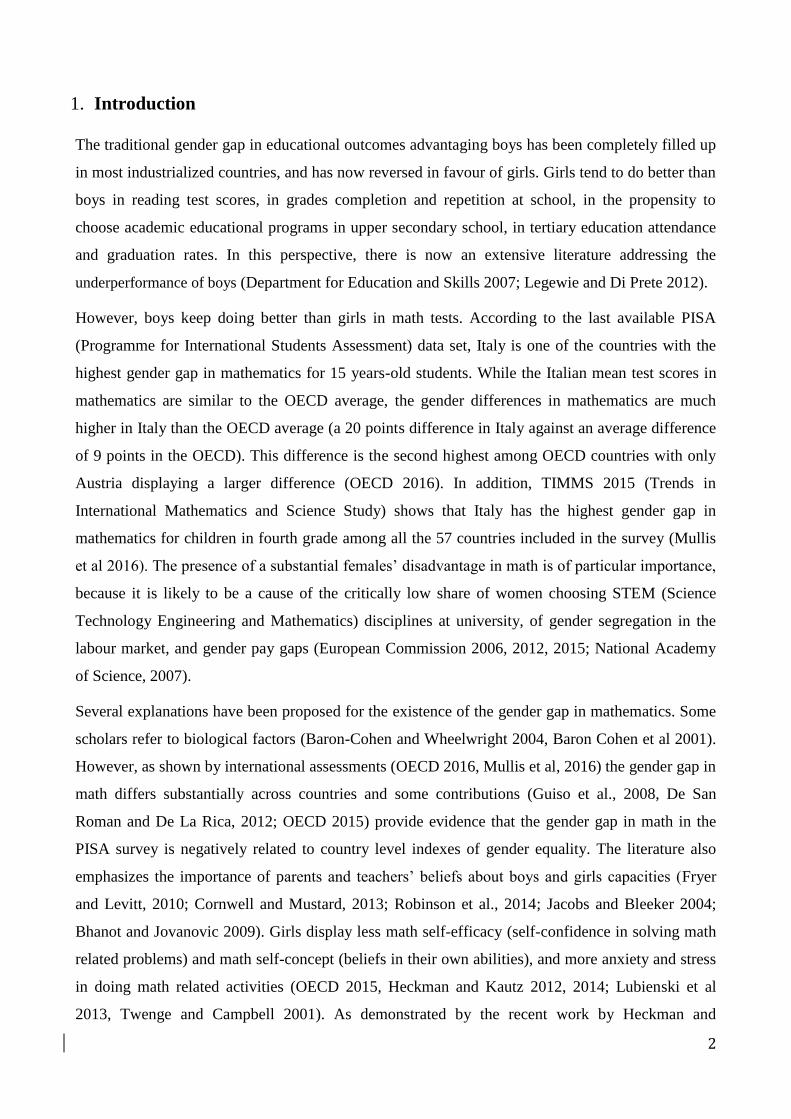
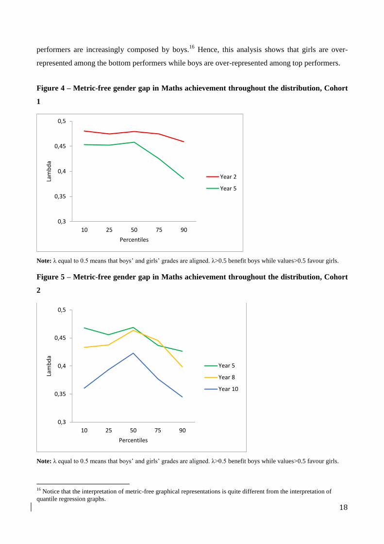
performing students relative to low performing students. Figures 4 and 5 present metric-free
measures of the math gender gap throughout the test scores distribution in years 2, 5, 8 and 10.
Values of below 0.5 indicate a boys‟ advantage, while values above 0.5 indicate a girl‟s
advantage. Figures 2 and 3 show that the gap favours males at all percentiles in all school years.
Girls are always over-represented at the bottom of the distribution and under-represented at the top
of the distribution. For instance, consider Cohort 1-year 5. 10 is equal to 0.45, meaning that if girls
and boys where equal in number, the bottom 10% of the distribution would be composed by 45% of
boys and 55% of girls. Instead, 90 is equal to 0.38: hence, with an equal share of boys and girls the
top 10% of the distribution would be composed by 38% of girls and 62% of boys.
In years 2 and 5 the girls‟ disadvantage is moderate at low percentiles and increases at high
percentiles (meaning that the better performing children are mostly boys). Instead, the difference is
very strong at both the bottom and the top of the distribution in years 8 and 10, indicating that as we
move further from the median, bottom performers are increasingly composed by girls, and top
-0,45
-0,4
-0,35
-0,3
-0,25
-0,2
-0,15
-0,1
-0,05
0
10 25 50 75 90
Percentiles Year 5
Year 8
Year 10
18
performers are increasingly composed by boys.16
Hence, this analysis shows that girls are over-
represented among the bottom performers while boys are over-represented among top performers.
Figure 4 – Metric-free gender gap in Maths achievement throughout the distribution, Cohort
1
Note: λ equal to 0.5 means that boys‟ and girls‟ grades are aligned. λ>0.5 benefit boys while values>0.5 favour girls.
Figure 5 – Metric-free gender gap in Maths achievement throughout the distribution, Cohort
2
Note: λ equal to 0.5 means that boys‟ and girls‟ grades are aligned. λ>0.5 benefit boys while values>0.5 favour girls.
16
Notice that the interpretation of metric-free graphical representations is quite different from the interpretation of
quantile regression graphs.
0,3
0,35
0,4
0,45
0,5
10 25 50 75 90
Lam
bd
a
Percentiles
Year 2
Year 5
0,3
0,35
0,4
0,45
0,5
10 25 50 75 90
Lam
bd
a
Percentiles
Year 5
Year 8
Year 10

19
How does the gender gap evolve as children grow older? The relative position of girls over boys
deteriorates substantially between years 2 and 5 (i.e. throughout elementary school). Instead, there
is only a small change between years 5 and 8 (middle school), while the girls‟ disadvantage sharply
increases again between years 8 and 10 (after tracking, in the first two years of high school). These
results are not dissimilar from the findings from the regression models on test scores, and as we will
see below, are highly consistent with the results of the dynamic model estimation.
4.3 Dynamic model estimation
As shown in Table 1, we only have data for a limited number of school years within each cohort.
For the estimation of the dynamic model with the pseudo-panel strategy described in section 3.3,
there is an additional limitation, because the month of birth – the instrumental variable necessary for
model identification – is not available for all assessments. Hence, we have little leeway in the
choice of the cohorts: (i) for the analysis of the evolution between years 2 and 5 we use the cohort
attending year 1 in 2010-11; (ii) for the analysis of the evolution between years 5 and 8 we use the
cohort attending year 1 in 2007-08; (iii) for the analysis of the evolution between years 8 and 10 we
use the cohort attending year 1 in 2005-06.
Table 4 summarizes the results for the gender coefficient17
. Columns labelled “CS” include the
estimates of the gender coefficient from cross-sectional models, while columns labelled “Dyn”
report the corresponding coefficients for dynamic models.
Table 4 – Results of the pseudo-panel estimation. Cross sectional and dynamic models
estimates
Between 2° and 5°
grade
Between 5° and 8°
grade
Between 8° and 10°
grade
Cohort year 1
in 2010-11
Cohort year 1
in 2007-08
Cohort year 1
in 2005-06
Y-2
CS
Y-5
CS
Y-5
Dyn
Y-5
CS
Y-8
CS
Y-8
Dyn
Y-8
CS Y-10
CS Y-10
Dyn Female -0.093
***
-0.194
***
-0.145
***
-0.180
***
-0.145
***
-0.029
ns
-0.222
***
-0.358
***
-0.151
***
Month of birth -0.031
***
-0.017
***
-0.016
***
-0.010
***
-0.005
**
-0.005
**
PredictedY1_lag 0.536
***
0.644
***
0.932
**
N 25752 18051 18051 24617 21586 21586 21149 18274 18274
Notes. Pseudo-panel estimates are grey-shadowed.
- CS=cross-sectional model. Dyn=dynamic model. Lag y# = lagged value is the predicted scores at year #.
- * indicates that the underlying coefficient is significant at 10% level, ** at 5% and ***1%.
- All models include macro-area of residence, maternal and paternal education.
17
Full estimates are in appendix A, table A4.

20
- Children anticipating enrolment before the regular grade and children enrolled in lower grades are not included.
- Month of birth measured as: January=1, February=2…December=12.
In the dynamic models, the coefficients represent the extent to which the achievement growth
between two consecutive assessments differs between girls and boys, given test scores at the
previous assessment (in other words, the difference between girls and boys in the second
assessment when comparing a girl and boy displaying the same performance in the previous
assessment).
We observe a widening gap between girls and boys between years 2 and 5. When comparing a boy
and a girl with the same individual characteristics and same performance in second grade, by the
end of fifth grade the boy will score on average 0.145 standard deviations more than the girl.
The gap keeps increasing between years 5 and 8 (the coefficient estimate is -0.029, implying that
the girls would lose on average an additional thirtieth of a standard deviation), but the estimate is
not statistically significant. Thus, we conclude that the gap does not evolve much in middle school.
Interestingly, if we had interpreted the evolution based on the comparison of the corresponding
cross-sectional coefficients (-0.180 in year 5 vs. -0.145 in year 8), we would have inferred a
reduction of the gender gap (see section 3,3 for a discussion on this point). Notice that this result is
consistent with the results shown by De Simone (2013) and based on the TIMSS assessment, who
finds that the gender gap in math in Italy does not widen between years 4 and 8.18
Once we analyse the evolution between years 8 and 10, we find another substantial deterioration of
girls‟ achievements (girls lose -0.151 points relative to equally performing boys in year 8).
However, the coefficient of the month of birth decreases substantially as children grow older, and
appears much lower at year 8 than in earlier grades. Since the reliability of the estimates depends on
the predictive power of the instrument, caution should be used when interpreting this estimate.19
Overall, dynamic modelling shows that the distance between girls and boys widens substantially in
elementary school, remains basically stable during middle school and starts widening again in high
school. Interestingly, these results are fully consistent with our robust findings from the metric-free
analyses.
5. Summary and conclusions
In this paper, we conduct a detailed analysis of the gender gap in math test scores in Italy, one of the
countries in the OECD displaying the largest differential between boys and girls in the PISA
18 Notice however that De Simone (2013) does not address the issue of the need of an instrumental variable to ensure identification, while in this paper we use the month of birth. 19
These considerations stem from the results of an extensive simulation study in Contini and Grand (2015), who study
the reliability of the estimates for different predictive power of the instrument and sample sizes.

21
assessment. We have employed cross sectional data from an Italian national learning assessment
from 2010 to 2015, testing children in selected grades from second to tenth grades. Given the lack
of longitudinal data, we analyse the data by cohort relying on repeated assessments of the same
cohort of students (although not the same specific students).
First, we describe the gender gap in standardised test scores for all the available cohorts and we see
that the gender gap is always in favour of boys. Second, we estimate the magnitude of the
standardized gender gap using OLS regression, and school and province fixed-effect models for two
of the longest available cohorts, separately. Our results show that girls systematically underperform
boys, even after controlling for individual and family background characteristics. We also find that
the gap is larger for those children whose mothers have a high school or university degree.
Third, we analyse the gap throughout the test scores distribution using quantile regression, and
show that the gap is generally larger at the top of the performance distribution.
Fourth, we re-analyse the gap throughout the test scores distribution using metric-free methods. As
expected, girls are over-represented among the bottom performers while boys are over-represented
among top performers. By comparing children in different school years, we observe very clearly
that the gender gap widens substantially as children progress in school. In particular, inequalities
rise sharply between grades 2 and 5 (elementary school), do not evolve much between grades 5 and
8 (middle school), and rise again after year 8, when students are in high school.
Finally, we estimate dynamic models relating the average math performance at two consecutive
assessments, allowing estimating genuine new gender inequalities developed between two
consecutive surveys. Lacking longitudinal data, we have used a pseudo-panel imputed regression
technique. Our findings point to the existence of mechanisms making girls losing ground relative to
boys between years 2 and 5 and between year 8 and 10, while we do not observe a widening gap
between years 5 and 8. These findings are fully consistent with the metric-free results.
Overall, our findings confirm previous results from the US data, that the gender gap exists at an
early age (in grade 2 for Italy) and it increases in older grades. Our paper represents the first
systematic account of gender inequalities in math achievement in Italy.
As highlighted in the introduction, gender related stereotypes are likely to play a major role in the
differences between girls and boys cognitive outcomes, both in maths and scientific subjects (where
girls are disadvantaged) and reading literacy (where boys are disadvantaged). The analysis of the
reasons why the gender gap in maths exists and how it can be reduced is beyond the scope of our
contribution. Nevertheless, even if Italy is one of the countries with worst performances in terms of

22
gender equality within the European union (EIGE 2015), gender equality is not explicitly expressed
as a goal for the school system and it is not incorporated into legal documents or official regulations
for education until 2015 (Eurydice 2010a, 2010b, Biemmi, 2015). The school reform of 2015
contains an article (Law n.107, 13 July 2015, art. 1, 16) that aimed to promote gender equality and
to prevent gendered violence but this article has not been implemented yet. Our paper, providing
extensive evidence of the existence of a gender gap since an early age and of its increase during
childhood, points to the need of the introduction of gender equality policies in the Italian
educational system. Given that the gap is smaller in primary school respect to older grades, the
policy intervention would be more cost efficient if it started addressing young children.
References
Angrist, J., E. Battistin, and D. Vuri (2015). In a Small Moment: Class Size and Moral Hazard in
the Mezzogiorno. IZA Discussion Paper No. 8959.
Ballatore, R., Paccagnella, M., Tonello, M. (2015) Bullied because younger than my mates?The
effect of age rank on victimization at school∗. Bank of Italy Working paper. Available at: https://www.bancaditalia.it/pubblicazioni/altri-atti-convegni/2016-human-capital/Ballatore_Paccagnella_Tonello.pdf
Baron-Cohen S, Wheelwright S, Skinner R, Martin J, Clubley E. (2001) The autism-spectrum
quotient (AQ): evidence from Asperger syndrome/high-functioning autism, males and
females, scientists and mathematicians. J Autism Dev Disord.; 31(1):5-17.
Bedard, K. & Cho, I. (2010) Early gender test score gaps across OECD countries, Economics of
Education Review 29, 348–363
Bertoni, M., G. Brunello, and L. Rocco (2013). When the cat is near the mice won‟t play: the effect
of external examiners in Italian schools. Journal of Public Economics 104, 65-77.
Bhanot, R. T., & Jovanovic, J. (2009). The links between parent behaviors and boys‟ and girls‟
science achievement beliefs. Applied Developmental Science, 13 (1), 42-59.
Biemmi I. (2015) Gender in schools and culture: taking stock of education in Italy, Gender and
Education, 27:7, 812-827, DOI: 10.1080/09540253.2015.1103841
Boaler, J. (2002). Paying the price for „sugar and spice‟: shifting the analytical lens in equity
research. Mathematical Thinking and Learning, 4(2&3), 127-144.
Boaler, J, Altendorff, L. & Kent, G. (2011). Mathematics and science inequalities in the United
Kingdom: when elitism, sexism and culture collide. Oxford Review of Education, 37(4),
457-484.
Blossfeld, H.-P., von Maurice, J. & Schneider, T. (2011). The National Educational Panel Study:
need, main features, and research potential. In H.-P. Blossfeld, H.-G. Roßbach & J. von
Maurice (Eds.), Education as a Lifelong Process - The German National Educational Panel
Study (NEPS). (Zeitschrift für Erziehungswissenschaft; Special Issue 14) (pp. 5-17).
Heidelberg: VS Verlag für Sozialwissenschaften.
Buckles K.S. and Hungerman D.M. (2013) Season of Birth and Later Outcomes: Old Questions,
New Answers. The Review of Economics and Statistics 95 (3), pp. 711-724

23
Carlana M. La Ferrara E. and Pinotti P. (2016) Shaping Educational Careers of Immigrant Children:
Aspirations, Cognitive Skills and Teachers‟ Beliefs, mimeo, Bocconi University
Checchi, D., Fiorio, C.V. and Leonardi, M. (2013), “Intergenerational Persistence of Educational
Attainment in Italy”, Economics Letters, 118, pp. 229-232.
Choi, Á, Gil, M. Mediavilla M. and Valbuena, J.(2016a), Double Toil and Trouble: Grade Retention
and Academic Performance (March 9, 2016). IEB Working Paper N. 2016/07. Available at
SSRN: https://ssrn.com/abstract=2745970
Choi, Á, Gil, M. Mediavilla M. and Valbuena, J.(2016b) The evolution of educational inequalities
in Spain: dynamic evidence from repeated cross-sections, IEB Working Paper N. 2016/25
Cornwell C., Mustard D. (2013) Non-cognitive Skills and the Gender Disparities in Test Scores and
Teacher Assessments: Evidence from Primary School. The Journal of Human Resources 48:
236-264.
Contini D. & Grand E. (2015). On Estimating Achievement Dynamic Models from Repeated Cross-
Sections. Sociological Methods and Research, doi: 10.1177/0049124115613773.
Crawford, C., Dearden, L. and Greaves, E. (2013) When you are born matters: evidence for
England. Report R80. Institute for Fiscal Studies, London.
Crawford, C., Dearden, L. and Meghir, C. (2007)When you are born matters: the impact of date of
birth on child cognitive outcomes in England. Report. Centre for the Economics of
Education, London.
Crawford, C., Dearden, L., Greaves, E. (2014) The drivers of month-of-birth differences in
children‟s cognitive and non-cognitive skills. Journal of Royal Statistical Society 177, 829-
860.
Department for Education and Skills (2007). Gender and education: the evidence on pupils in
England,http://webarchive.nationalarchives.gov.uk/20090108131525/http:/dcsf.gov.uk/researc
h/data/uploadfiles/rtp01-07.pdf
De San Román, A. G, & de La Rica Goiricelaya, S. (2012). Gender gaps in PISA test scores: the
impact of social norms and the mother‟s transmission of role attitudes. IZA Discussion
Paper 6338.‟
De Simone, G. (2013). Render unto primary the things which are primary's: Inherited and fresh
learning divides in Italian lower secondary education. Economics of Education Review,
35(C), 12-23.
De Simone G. and A. Gavosto (2013), “Patterns of Value-Added Creation in the Transition from
Primary to Lower Secondary Education in Italy”, FGA Working Paper n. 47/2013
EIGE (2015), Gender Equality Index 2015- Italy, European Institute for Gender Equality, Vilnius.
Eurydice. 2010a. Gender Differences in Educational Outcomes: A Study on the
Measures Taken and the Current Situation in Europe . Brussels: Education, Audiovisual and
Culture Executive Agency.
Eurydice. 2010b. Gender Differences in Educational Outcomes: A Study on the
Measures Taken and the Current Situation in Europe – Italy. Brussels: Education,
Audiovisual and Culture Executive Agency.
European Commission 2006, Women in Science and Technology- the Business Perspective,
Luxembourg: Office for Official Publication of the European Communities
European Commission 2012, Enhancing excellence, gender equality and efficiency in research and
innovation, Luxembourg: Office for Official Publication of the European Communities
European Commission 2015. Science is a girls‟ thing, Newsletter Nov. 2015 http://science-girl-

24
thing.eu/newsletters/november-2015.html
Fryer, Roland G., and Steven D. Levitt. 2010. "An Empirical Analysis of the Gender Gap in
Mathematics." American Economic Journal: Applied Economics, 2(2): 210-40.
Good, J. J., Woodzicka, J. A., & Wingfield, L. C. (2010). The effects of gender stereotypic and
counter-stereotypic textbook images on science performance. Journal of Social Psychology,
150 (2), 132-147.
Guiso L., Monte F., Sapienza P., & Zingales L. (2008). Culture, gender, and math. Science, 320
(5880), 1164–1165.
Heckman, J.J., Mosso, S. (2014). The Economics of Human Development and Social Mobility.
Annual Review of Economics 6, 689-733.
Heckman, J. J. & T. Kautz (2012). Hard evidence on soft skills. Labour Economics, 19, 451-464.
Heckman, J. J. & T. Kautz (2014). Fostering and measuring skills interventions that improve
character and cognition. In J. J. Heckman, J. E. Humphries, and T. Kautz (Eds.), The GED
Myth: Education, Achievement Tests, and the Role of Character in American Life, Chapter
9. Chicago, IL: University of Chicago Press.
Ichino A. Tabellini G. (2014) Freeing the Italian school system, Labour Economics, 30, 113–128.
Jacob, Brian and Jesse Rothstein. 2016. "The Measurement of Student Ability in Modern
Assessment Systems." Journal of Economic Perspectives, 30(3): 85-108.
Jacobs, J. E., & Bleeker, M. M. (2004). Girls‟ and boys‟ developing interests in math and science:
do parents matter? New Directions for Child and Adolescent Development, 106, 5-21.
Koenker , R., & Basset G. (1978) Regression Quantiles, Econometrica, Vol 46 (1), pp. 33-50.
Legewie, J., DiPrete, T. A. (2012). School Context and the Gender Gap in Educational
Achievement, American Sociological Review 77 (3): 463–85.
Lubienski, S., Robinson, J., Crane, C., Ganley, C. (2013) Girls' and Boys' Mathematics
Achievement, Affect, and Experiences: Findings from ECLS-K. Journal for Research in
Mathematics Education, 44, 634-645.
Lucifora, C.Tonello M. (2015), Cheating and social interactions. Evidence from a randomized
experiment in a national evaluation program, Journal of Economic Behavior &
Organization, 115, 45-66.
Mocetti, S. (2011). Educational choices and the selection process: Before and after compulsory
schooling. Education Economics, 20(2), 189–209.
Montanaro, P. (2008). Learning divides across the Italian regions: some evidence from national and
international surveys. Bank of Italy Questioni di Economia e Finanza (Occasional Papers)
No. 12.
Mullis, I. V. S., Martin, M. O., Foy, P., & Hooper, M. (2016). TIMSS 2015 International Results in
Mathematics. Retrieved from Boston College, TIMSS & PIRLS International Study Center
National Academy of Science (2007) Beyond Bias and Barriers: Fulfilling the Potential of Women
in Academic Science and Engineering (2007)
OECD. (2015). The ABC of Gender Equality in Education: Aptitude, Behavior, Confidence. PISA
Paris: OECD.

25
OECD (2016), PISA 2015 Results (Volume I): Excellence and Equity in Education, OECD
Publishing, Paris.
Paccagnella M., Sestito P. (2014), School Cheating and Social Capital, Education Economics,
22(4), 367-388
Penner, A.M., Parer M., (2008) Gender differences in mathematics achievement: Exploring the
early grades and the extremes Social Science Research 37 (1), 239-253
Pellizzari, A. and Billari, F. (2012) The younger, the better?: age-related differences in academic
performance at university. Journal of Population Economics, 25, 697–739.
Robertson, E. (2011) The effects of quarter of birth on academic outcomes at the elementary school
level. Economics of Education Review, 30, 300–31
Robinson Joseph P. and Lubiensky Sarah T. (2011) The Development of Gender Achievement
Gaps in Mathematics and Reading During Elementary and Middle School Examining Direct
Cognitive Assessments and Teacher Ratings. American Educational Resources Journal. 48,
2268-302
Robinson-Cimpian JP, Lubienski ST, Ganley CM, Copur-Gencturk Y (2014) Teachers' perceptions
of students' mathematics proficiency may exacerbate early gender gaps in achievement.
Development Psychology 50(4):1262-81. doi: 10.1037/a0035073.
Twenge, J. M., & W. K. Campbell. (2001). Age and birth cohort differences in self-esteem: a cross-
temporal meta-analysis. Personality and Social Psychology Review, 5(4), 735–748.
Verbeek, M. & Vella, F. (2005) Estimating dynamic models from repeated cross-sections, Journal
of Econometrics, 127, 83-102
Viteritti A (2009) A Cinderella or a Princess? The Italian School between Practices and Reforms.
Italian Journal of Sociology of Education, 3, 10-332
Zohar, A., & Sela, D. (2003). Her physics, his physics: gender issues in Israeli advanced placement
physics classes.” International Journal of Science Education, 25(2), 245-268.

26
Appendix
Table A1: Descriptive statistics (by cohort)
COHORT 1 COHORT 2
Gender
Male
Female
Missing
Year 5
0.51
0.49
Year 8
0.50
0.50
Year 10
0.50
0.50
Year 2
0.51
0.49
Year 5
0.50
0.50
ESCS index
Mean
Standard deviation
n.a.
n.a.
0.07
0.95
n.a.
0.06
1.01
Area of residence
North-West
North-East
Centre
South
Islands
0.18
0.20
0.21
0.22
0.19
0.19
0.20
0.19
0.23
0.19
0.27
0.27
0.30
0.22
0.13
0.08
0.18
0.21
0.21
0.21
0.19
0.17
0.20
0.17
0.26
0.20
Maternal education
Degree
High school
Middle school
Missing
0.13
0.32
0.38
0.17
0.13
0.30
0.35
0.22
n.a.
0.15
0.33
0.34
0.18
0.14
0.34
0.33
0.19
Paternal education
Degree
High school
Middle school
Missing
0.12
0.27
0.43
0.18
0.11
0.26
0.40
0.23
n.a.
0.12
0.28
0.40
0.20
0.11
0.29
0.40
0.20

27
Table A2 – Effect of other independent variables on achievements in Mathematics (OLS by cohorts)
COHORT 1 COHORT 2
Year 5 Year 8 Year10 Year 2 Year 5
Female -0.152 -0.184 -0.324 -0.088 -0.183
(0.011)*** (0.012)*** (0.012)*** (0.010)*** (0.013)***
Escs index n.a. n.a. 0.187 n.a. 0.136
(0.008)*** (0.011)***
Escs*Fem n.a. n.a. 0.042 n.a. -0.007
0.012)*** (0.013)
Region of residence
(ref NW)
NE -0.056 0.086 -0.009 -0.105 -0.031
(0.017)*** (0.019)*** (0.018) (0.017)*** (0.020)
Centre -0.125 -0.065 -0.416 -0.123 -0.139
(0.017)*** (0.019)*** (0.018)*** (0.016)*** (0.020)***
South -0.159 -0.215 -0.512 -0.106 -0.257
(0.016)*** (0.018)*** (0.017)*** (0.015)*** (0.018)***
Islands -0.305 -0.095 -0.555 -0.194 -0.388
(0.018)*** (0.019)*** (0.018)*** (0.017)*** (0.020)***
Maternal education
(ref University)
Middle school -0.369 -0.486 n.a. -0.301 -0.296
(0.021)*** (0.024)*** (0.020)*** (0.028)***
High school -0.132 -0.216 n.a. -0.088 -0.127
(0.020)*** (0.023)*** (0.018)*** (0.023)***
Missing -0.255 -0.277 n.a. -0.219 -0.150
(0.035)*** (0.035)*** (0.033)*** (0.039)***
Paternal education
(ref University)
Middle school -0.296 -0.334 n.a. -0.265 -0.132
(0.022)*** (0.025)*** (0.021)*** (0.028)***
High school -0.105 -0.090 n.a. -0.088 0.001
(0.021)*** (0.025)*** (0.020)*** (0.025)
Missing -0.336 -0.271 n.a. -0.290 -0.086
(0.034)*** (0.036)*** (0.033)*** (0.040)**
N 31,134 25,111 22,943 31,330 21,271
R2 0.068 0.081 0.156 0.048 0.102
Notes. Std errors are in brackets. * indicates that the underlying coefficient is significant at 5% level, ** at 1% and ***0.1%. Missing is a dummy variable equal 1 if the specific variable is missing; equal 0 otherwise.
Table A3 - The gender gap (G-B) in math test scores. OLS using raw % scores (by cohorts)
Year 2 Year 5 Year 8 Year 10
Cohort 1 n.a -0.028 -0.035 -0.079
(0.002)*** (0.002)*** (0.003)***
Cohort 2 -0.018 -0.035 n.a. n.a
(0.002)*** (0.002)*** Notes. Std errors are in brackets. * indicates that the underlying coefficient is significant at 5% level, ** at 1% and ***0.1%.

28
Table A4 Dynamic models estimation. Complete results.
Between 2° and 5°
grade
Between 5° and 8°
grade
Between 8° and 10°
grade
Cohort year 1
in 2010-11
Cohort year 1
in 2007-08
Cohort year 1
in 2005-06
Y-2
CS
Y-5
CS
Y-5
Dyn
Y-5
CS
Y-8
CS
Y-8
Dyn
Y-8
CS Y-10
CS Y-10
Dyn Female -0.093
(0.011)
***
-0.194
(0.014)
***
-0.145
(0.015)
***
-0180
(0.012)
***
-0.145
(0.013)
***
-0.029
(0.026)
-0.222
(0.013)
***
-0.358
(0.013)
***
-0.151
(0.091)
***
Month of birth -0.031
(0.002)
***
-0.017
(0.002)
***
-0.016
(0.002)
***
-0.010
(0.002)
***
-0.005
(0.002)
**
-0.005
(0.002)
**
PredictedY1_lag 0.536
(0.068)
***
0.644
(0.126)
***
0.932
(0.404)
**
Macro area
NW omitted
NE 0.004
(0.017)
0.053
(0.021)
**
0.051
(0.021)
**
0.031
(0.018)
*
-0.010
(0.019)
-0.030
(0.020)
0.081
(0.020)
***
0.020
(0.020)
-0.056
0.038)
Centre 0.043
(0.018)
**
-0.118
(0.021)
***
-0.141
(0.021)
***
-0.036
(0.018)
**
-0.159
(0.020)
***
-0.136
(0.020)
***
-0.102
(0.020)
***
-0.419
(0.020)
***
-0.323
(0.046)
***
South 0.081
(0.017)
***
-0.240
(0.020)
***
-0.283
(0.021)
***
-0.007
(0.017)
-0.279
(0.019)
***
-0.274
(0.019)
***
-0.255
(0.019)
***
-0.583
(0.019)
***
-0.345
(0.106)
***
Islands -0.022
(0.018)
-0.226
(0.023)
***
-0.214
(0.023)
***
-0.163
(0.018)
***
-0.237
(0.021)
***
-0.132
(0.030)
***
-0.121
(0.021)
***
-0.620
(0.021)
***
-0.508
(0.054)
***
Paternal educ
(University
omitted)
High school -0.125
(0.021)
***
-0.115
(0.024)
***
-0.048
(0.026)
*
-0.121
(0.023)
***
-0.149
(0.024)
***
0.071
(0.028)
**
-0.081
(0.026)
***
-0.033
(0.020)
0.042
(0.038)
Middle school -0.276
(0.022)
***
-0.296
(0.026)
***
-0.148
(0.032)
***
-0.327
(0.023)
***
-0.388
(0.025)
***
-0.178
0.048)
***
-0.319
(0.027)
***
-0.216
(0.021)
***
0.081
(0.130)
Missing -0.342
(0.038)
***
-0.254
(0.041)
***
-0.070
(0.047)
-0.325
(0.038)
***
-0.317
(0.036)
***
-0.107
(0.054)
**
-0.273
(0.039)
***
-0.359
(0.031)
***
-0.104
(0.114)
Maternal educ
(University
omitted)
High school -0.130
(0.019)
***
-0.179
(0.022)
***
-0.110
(0.024)
***
-0.140
(0.021)
***
-0.199
(0.022)
***
-0.108
(0.029)
***
-0.207
(0.025)
***
-0.101
(0.019)
***
0.092
(0.085)
Middle school -0.362
(0.021)
***
-0.444
(0.025)
***
-0.250
(0.034)
***
-0.401
(0.022)
***
-0.476
(0.024)
***
-0.218
(0.056)
***
-0.437
(0.026)
***
-0.275
(0.021)
***
0.133
(0.177)
Missing -0.168
(0.037)
***
0.206
(0.040)
***
-0.116
(0.042)
***
-0.243
(0.038)
***
-0.303
(0.036)
***
-0.147
(0.047)
***
-0.217
(0.039)
***
-0.278
(0.033)
***
-0.075
(0.093)
N 25752 18051 18051 24617 21586 21586 21149 18274 18274
R2 0.059 0.085 0.085 0.076 0.098 0.098 0.083 0.173 0.173
Notes. Std errors are in brackets. Pseudo-panel estimates are grey-shadowed.
- CS=cross-sectional model. Dyn=dynamic model. Lag y# = lagged value is the predicted scores at year #.
- * indicates that the underlying coefficient is significant at 10% level, ** at 5% and ***1%. - Children anticipating enrolment before the regular grade and children enrolled in lower grades are not included.
- Month of birth measured as: January=1, February=2…December=12.
- Missing is a dummy variable equal 1 if the specific variable is missing; equal 0 otherwise.


![Achievement Gap[1]](https://img.pdfslide.us/doc/110x75/55842058d8b42aa81e8b4931/achievement-gap1-5584b8761200b.jpg)