NASA Technical Memorandum 100746

The GEM-T2Gravitational Model

J.G. Marsh, E J. Lerch, B.H. Putney,T.L. Felsentreger, B.V. Sanchez,S.M. Klosko, G.B. Patel, J.W. Robbins,R.G. Williamson, T.E. Engelis, W.E Eddy,N.L. Chandler, D.S. Chinn, S. Kapoor,K.E. Rachlin, L.E. Braatz, and E.C. Pavlis

October 1989

N/ A(NASA-TM-lO0746_ THE G_M-T2 GRAVITATIONAL N90-1_984MO_:EL (NASA) 91 p CSCL 0BE

Uncl as

G3/46 0239Z69

https://ntrs.nasa.gov/search.jsp?R=19900003668 2018-05-26T23:33:16+00:00Z

NASA Technical Memorandum 100746"!

?

The GEM-T2Gravitational Model

•_ J.G. Marsh, F.J. Lerch, B.H. Pumey,

T.L. Felsentreger, B.V. Sanchez

Goddard Space Flight Center

Greenbelt, Maryland

S.M. Klosko, G.B. Patel, J.W. Robbins,

R.G. WiUiamson, T.E. Engelis, W.F. Eddy,N.L. Chandler, D.S. Chinn, S. Kapoor,

K.E. Rachlin, L.E. Braatz

ST Systems CorporationLanham, Maryland

E. C. Pavlis

University of MarylandCollege Park, Maryland

. National Aeronautics andSpace Administration

Goddard Space Flight Centeri Greenbelt, MD

1989

',i_: _, ABSTRACT

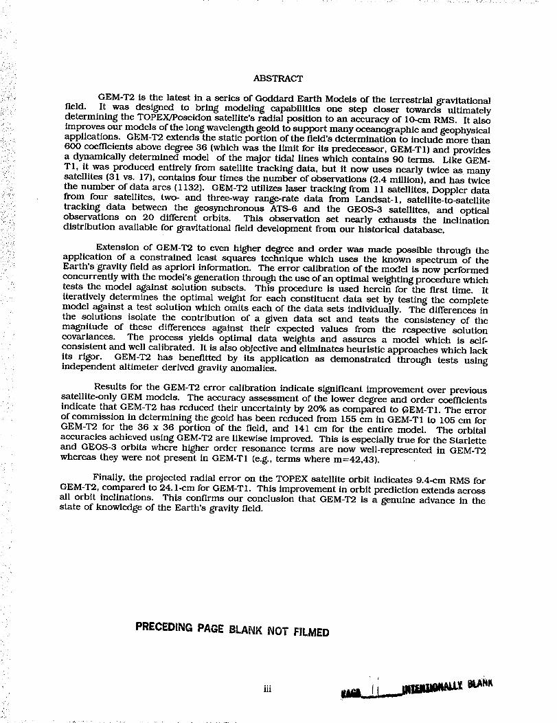
,_iii_,, GEM-T2 is the latest in a series of Goddard Earth Models of the terrestrial gravitational_, field. It was designed to bring modeling capabilities one step closer towards ultimately_' determining the TOPEX/Poseidon satelllte's radial position to an accuracy of 10-cm RMS. It also

: improves our models of the long wavelength geotd to support many oceanographic and geophysicali:_:: applications. GEM-T2 extends the static portion of the field's determination to include more than_ 600 coefficients above degree 36 (which was the limit for its predecessor, GEM-T1) and provides(_. :L

_ a dynamically determined model of the major tidal lines which contains 90 terms. Like GEM-;_ T1, it was produced entirely from satellite tracking data, but it now uses nearly twice as many"__ii_! satellites (31 vs. 17), contains four times the number of observations (2.4 million), and has twice

the number of data arcs (1132). GEM-T2 utilizes laser tracking from 11 satellites, Doppler data_'_ from four satellites, two- and three-way range-rate data from Landsat-1, satellite-to-satellite!iii_ tracking data between the geosynchronous ATS-6 and the GEOS-3 satellites, and optical

observations on 20 different orbits. This observation set nearly exhausts the inclination':'_: distribution available for gravitational field development from our historical database.

Extension of GEM-T2 to even higher degree and order was made possible through theapplication of a constrained least squares technique which uses the known spectrum of the

_ii!i/_ Earth's gravity field as aprlorl information. The error calibration of the model is now performed' concurrently with the model's generation through the use of an optimal weighting procedure which

tests the model against solution subsets. This procedure is used herein for the first time. Ititeratively determines the optimal weight for each constituent data set by testing the complete

• model against a test solution which omits each of the data sets individually. The differences inthe solutions isolate the contribution of a given data set and tests the consistency of themagnitude of these differences against their expected values from the respective solution

:: covariances. The process yields optimal data weights and assures a model which is self-consistent and well calibrated. It is also objective and eliminates heuristic approaches which lackits rigor. GEM-T2 has benefitted by its application as demonstrated through tests using

:, independent altimeter derived gravity anomalies.

Results for the GEM-T2 error calibration indicate significant improvement over previousi satellite'only GEM models. The accuracy assessment of the lower degree and order coefficients

indicate that GEM-T2 has reduced their uncertainty by 20% as compared to _EM-T1. The errori of commission in determining the geoid has been reduced from 155 cm in GEM-T1 to 105 cm for

GEM-T2 for the 36 x 36 portion of the field, and 141 cm for the entire model. The orbitalaccuracies achieved using GEM-T2 are likewise improved. This is especially true for the Starletteand GEOS-3 orbits where higher order resonance terms are now well-represented in GEM-T2whereas they were not present in GEM-T1 (e.g., terms where m=42,43).

• . Finally, the projected radial error on the TOPEX satellite orbit indicates 9.4-cm RMS forGEM-T2, compared to 24.1-cm for GEM-T1. This improvement in orbit prediction extends acrossall orbit inclinations. This confirms our conclusion that GEM-T2 is a genuine advance in thestate of knowledge of the Earth's gravity field.

PRECEDINGPAGEBLANKNOT FILMEDi:

• i Z

111 _[____lpl

)

SECTION 1. INTRODUCTION

" :_:i_

:_i::_ Goddard Earth Model (GEM) -T2 is the latest in a series of improved gravitational models_:,i developed at NASA/GOddard Space Flight Center using supercomputer capabilities, modern

geodetic constants and reference parameters, and a new optimum data weighting and error_:_ calibration technique (Lerch, 1989) for its determination. GSFC has undertaken an effort,

requiring both pre- and post-launch activities, to develop force models capable of supporting theorbital positioning and geoid accuracy required for the TOPEX/Poseidon mission. GEM-T2, likeits predecessor GEM-TI (Marsh et al., 1987, 1988), has been determined solely from satellite

_: tracking data. The solution for the Earth's geopotential field, both static and tidally induced,_il_._ ' has been extended to higher degree and order in GEM-T2. The static geopotential is complete

for many orders to degree 50 to better accommodate zonal, low-order and satellite orbital_ resonance effects. The gravitational model has increased in size by'more than 600 coefficients:..... beyond the 36 x 36 solution of GEM-T1. The GEM-T2 tidal model includes adjustment for 90

harmonics (as compared to 66 coefficients in GEM-TI) distributed over 12 major tides which aresolved in the presence of a comprehensive ocean tidal model containing long wavelengthinformation for 32 major and minor constituents. This ocean tidal model contains over 600coefficients and was developed to provide a much more complete description of the longwavelength ocean tides to improve the separation of static and temporally varyinggravitational effects. Such a model is needed as described in Christodoulidis et al., (1988).

In accordance with the plans described in Marsh et al., (1987), Goddard Space FlightCenter has been approaching the gravity modeling problem in progressive stages. Each of theavailable satellite tracking, surface gravimetric and altimeter observation subsets is beingevaluated and qualified for its inclusion within the GEM models. As a prelude tocombination models which contain mixed and subtly incompatible types of observations (i.e.

mixing large numbers of satellite tracking observations with those provided by surface,, gravimetry and satellite altimetry which have a different bandwidth of field sensitivity), we find

it desirable to develop preliminary models which are largely free of these concerns. These"$,_tellite-only" models, like GEM-T1 and now GEM-T'2, are then thoroughly evaluated, optimizedand calibrated (Lerch et al., 1988) to better understand their accuracies and limitations. Much

!• of the error calibration for GEM-T2 is built into the solution through our application of anIterative optimal data weighting technique. By design, this method yields a well calibrated result.

Satellite tracking data provides the most unambiguous available measure of the longwavelength geopotentlal. A large historical database spanning all of the major trackingtechnologies has been developed at GSFC. Altimetry and surface gravimetry are known to havemodeling inaccuracies and inadequacies when describing the long wavelength geoid, andthese two surface data types are not strictly compatible with the attenuated gravitationalsignal seen from an evaluation of perturbed orbital behavior within tracking data.

. Therefore, in our approach, larger comprehensive models using surface gravimetry and altimetry.... are based on these "satellite-only" fields. A 50 x 50 combination model called GEM-T3 is under

•development with a preliminary version, PGS-3337 now available (Marsh et al, 1989a).Altimetry and surface gravimetry will be contained within GEM-T3 and will provide anexcellent resource for directly mapping the short wavelength geopotential over regions wherethese data are available. Furthermore, by progressively developing more complete andcomplex fields in a systematic way based upon well-calibrated base models, fieldoptimization is more readily attained, data incompatibilities are more easily located and reliable

_: _ments of the solution's uncertainties are obtained.

When beginning our most recent GEM modeling activities in 1984, an improved set ofEarth constants and reference frame parameters were incorporated. The solutions are

••:_i based on the state-of-the-art in satellite geodesy in the 1984-5 tlmeframe. The constants:: described for use in the MERIT Campaign (Melbourne et al., 1983) provided the starting pointi•::, for this assessment. The adoption of these values (which will be reviewed in Section 2.) and_: their uniform application across all tracking technologies, laid the foundation in achieving

:i the higher accuracy found in our most recent GEM-T1 and -T2 solutions. Of equal or greater

I

importance was the development of the optimal data weighting algorithms, improved_ solution calibration/testing methods, and the overall extension of the models to higher degree_, and order.

• Extending the model to high degree and order has been a very importantdevelopment in our latest models. This reduces the errors resulting from spectral leakagecoming from the omitted portion of the gravitational field beyond the limits of the recovered

: : model. By necessity, all omitted terms are implicitly assumed to have zero values. The GEM-T2.... model has been solved to as high a degree and order as necessary to exhaust the attenuated

gravitational signal contained in the tracking data. A constrained least squares solution(Lerch et al., 1979) is used to stabilize the behavior of the solution at high degree and order

_: where correlation and small data sensitivities are a problem. The availability of the:, • Cyber-205 supercomputer greatly increased our capabilities for extending the field size

and developing solution optimization techniques.

The major advancements of GEM-T2 over "its predecessor, GEM-T1, include:

• (a) the near-doubling of the number of distinct orbits sampled to form themodel. GEM-T1 used tracking data from 17 satellites. GEM,T2 contains contributions

from 31. The major new observation subsets include TRANET Doppler data acquiredon the polar NOVA-1 satellite, Unified S-Band average range-rate tracking onLandsat-l, laser data on the Japanese Ajisai satellite, satellite-to-satellite range-ratedata taken from the geosynchronous ATS-6 to GEOS-3, nine additional optical

• satellites and TRANET Doppler data taken on GEOSAT.

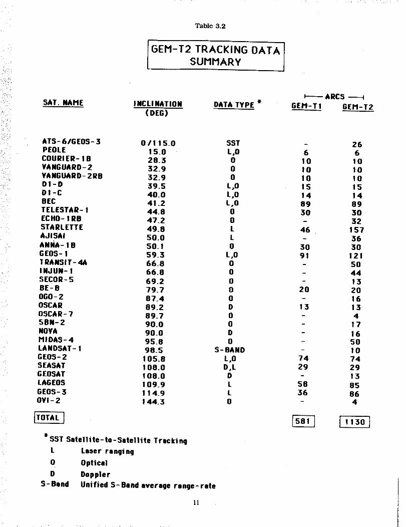
(b) the data set for GEM-T2 has also more than doubled. GEM-T1 was determinedusing 793,900 observations contained within 581 individual orbital arcs whereasGEM-T2 contains 2,386,000 observations from 1130 arcs.

(c) there has been a significant improvement in the laser data set utilized withinGEM-T2. Third-generation laser data from the 1980 and 1981 time periods has been

included from both GEOS-1 and GEOS-3. This represents a substantial upgrading ofthe information available from these satellites as compared to the 1975 to 1977data utilized in GEM-TI. These satellites are similar in inclination to that nominallyproposed for TOPEX/Poseidon and will strengthen the model when determiningprecise TOPEX/Poseidon ephemerides. LAGEOS ranging has been extended by nearly 3years to include the global data taken during 1984, 1985, 1986 and the first 2 months

of 1987. Likewise, ranging on Starlette has been extended to include data taken during1984 and 1986, and the 1500-km orbit of Ajisai is also included.

(d) there has been a major advance in our solution technique through theintroduction of an optimal data weighting and automatic error calibration approach. Theseproducts are now an integral part of the estimation procedure.

i (e) GEM-T2 is a significant improvement over GEM-TI both in terms of its geoidrepresen_tational accuracy and in its satellite orbit modeling uncertainties. This isespecially true in terms of its predicted performance on TOPEX/Poseidon's radialaccuracy using covariance propagations.

All of these issues, including in particular, a thorough error assessment of GEM-T2, willbe described in detail within this report.

i ¸

i SECTION 2. REFERENCE PARAMETERSi

A terrestrial gravity field solution must be defined within a well understood reference

: ii system. The dynamic satellite orbit computations are connected to ground-based observers• through these definitions. The orbital trajectories are integrated in the Conventional

Inertial Reference System (CIRS) which needs to be connected in time to theConventional Terrestrial Reference System (CTRS) which is realized by the global network of

..... Earth-fixed tracking stations. Application of terrestrial gravitational accelerations along thei_: i orbit are made using these same transformations.

Since 1979, the tracking data themselves have been sufficiently robust to allow a directadjustment of the geocentric station locations, the Earth's polar motion and the change in thelength of day {using 5-day averaging intervals) which provides a satellite-based definition of the

• CTRS. This system is dominated or exclusively based on the satellite laser ranging acquiredon the high-altitude LAGEOS satellite. Within GEM-T1 and GEM-T2, we have adjusted the Earth

_ i orientation parameters as part of the solution. This was desirable since we have moved ourdefinition of the CTRS to a new terrestrial origin {i.e., we are using a "zero-mean" definition for

_ polar motion based on LAGEOS and have transformed the historical Bureau International del'Heure (BIH) series which is referred to CIO into this new system; see Marsh et al., 1987, 1988).

i There is a near-singularity when simultaneously defining the satellite's right ascension of theascending node and UT1 using laser data given the weak sensitivity of the orbit to shortwavelength longitudinal gravity signals. The orbit can be rotated in longitude by 30-100m withlittle change in field performance. A change in UT1 of the same magnitude has the same effect.Thereby, the BIH definition of UT1 is adopted at the epoch of each 30-day LAGEOS orbit. Thelaser data then yields a well resolved measure of the change in length of day based on thisBIH origin. The adopted tidal variations in the Earth rotation (UT1) series are those of Yoder etel., {1981).

The laser station coordinates which are utilized are from the GSFC LAGEOS SL6(Christodoulidis et al., 1986) and SL7.1 {Smith et al., 1989 in press) solutions. The lasercoordinate network is rotated through a fixed angle {defined by the offset of CIO with respectto our new terrestrial origin) yielding a consistent definition of geodetic latitude for the siteswithin our new CTRS. We have tied non-laser tracking systems into this definition of CTRSusing a series of transformations and analyses as described in Marsh et al., {1987; Chapter6).

The J2000 Reference System with its associated DE200/LE200 planetary ephemeris formsthe basis for our CIRS definition. This connects the CTRS series in time using the nutationseries of the IAU 1980 provided by Wahr {1979) and the IAU 1976 precession series developedby Lieske (1976)

As the accuracy of tracking instruments has evolved, the requirements foraccurate reference frame definitions and consistent constants have become much more stringent.

, Physical models of increasing complexity are required to both exploit and explain these veryprecise satellite measurements. The advance of satellite geodesy has been oriented towardsamplifying the science yield from increasingly more accurate data, and in parallel, developing

,_'• newer tracking systems which permit more complex natural phenomena to be modelled. Forthe problem of determining a gravitational model, the solution output is a mathematical modelof a physical phenomenon whose empirical coefficients taken individually are not directly

• observed. Thereby, complex geophysical interpretations of the GEM gravitational models aredifficult unless strict attention is paid to these fundamental definitions. Errors in thesemodels or neglected effects cause problems in the definition and interpretation of these fields.

• For example, this is important in advanced analyses like those in physical oceanographywhere the GEM geoid is used to isolate non-gravitational signals exhibited by the oceantopography. For this reason we have taken great care in selecting the reference framedefinition and constants for the recent GEM solutions.

i

!

i' 3

:/

• :_ ,_.i¸¸

_: The following table lists the values adopted for the constants that enter into the models: used to create GEM-T2. 0nly the most important ones have been included. We have also

avoided repeating numbers which are implicitly embedded in well-known standard models

which are referenced and adopted in the whole (e.g., the constants describing the Wahrnutation model or Lieske's expressions for the precessional matrix).

2.1 Astronomical Constants

Speed of Light 299792458 m/sEquatorial radius of the Earth 6378137 mFlattening of the Earth 1/298.257Mean spin rate of Earth 0.00007292115 rad/sGeocentric Gravitational Constant 398600.436 km3/s 2Moon-Earth mass ratio 0.012300034Astronomical unit 149597870660 mSun-Earth mass ratio 332946.038

: _ 2.2 Dynamical Models

Static Geopotential Adjusting, GEM-T1 aprioriSolid Earth Tides Wahr (1979)Ocean Tides GEM-T1 apriori with 90

adjusting coefficientsRadiation pressure at I AU 0.0000045783 kg/m/s 2

o radiation pressure eoemcient adjustedAtmospheric Drag Jacchia (1971) with daily

values of F10.7 and Kp fluxo atmospheric drag coefficient adjusted; nominally once/day

i

' 2.3 Measurement Models

2.3. I Optical Data

parallactic refracti,on Hotter (1968)annual abberation "

i diurnal abberation "

precession/nutation of images Wahr/Lieske_ proper motions Hotter (1968)' i:' satellite clock corrections APL provided values

for active satellites

4

2.3.2 TRANET Doppler Data

Time tag correction from WWV O_I'oole (1976)Tropospheric refraction Modified Hopfleld Model of

Goad (Martin et al., 1987)Ionospheric refraction First-order correction

obtained from difference

of 150- and 400-MHz freq.Frequency bias correction pass-by-pass bias adjustment

2.3.3 Laser Range Data

Pre- and post-pass range Figgatte and Polesco (1982)calibrations

Tropospheric refraction Marinl and Murray (1973)

2.3.4 S-band Average Range-rateData

Tropospheric refraction Modified Hopfleld Model ofGoad (Martin et al., 1987)

Ionospheric refraction noneAntenna axis offset correction Gross (1968)/Martin et aL,

for non-az/el mounts (1987)

2.4 Reference System

CIRS J2000.0

Planetary Ephemeris JPL DE200Terrestrial time scale UTC (USNO)Precession IAU 1976 (Lieske, 1976)Nutation IAU 1980 (Wahr, 1979)

CTRS Lageos global solutionSL6 rotated to

"zero-mean" system

5

I

_,_ i_ _

SECTION 3. THE GEM-T2 OBSERVATIONS

The tracking observations available for gravitational modeling span 30-years of technologychange. These data contain a wide range of data precision and sophistication. The earliestobservations were taken at moments of opportunity when satellites or their rocket bodyfragments were illuminated by the sun, yet visible to a pre-dawn or alter-dusk shrouded Earthobserver. The satellite was photographed against the star background and positioned withina celestial system yielding a satellite right ascension and declination in the reference systemof the FK4 star catalogue. These images were capable of locating the sateIIite's direction

_' vis-a-vis the observer to a precision of one to two topocentric seconds of arc which for mostsatellite altitudes translated into positioning of approximately 10-meters.

Today's tracking technologies have advanced enormously, with active laser ranging systemstracking passive orbiting targets during day or night with single shot precision, which for the bestsystems, have sub-centimeter noise levels.

However, even for the extensive laser network now deployed to support theNASA/Crustal Dynamics Program and the European Wegener/Medlas activities, the fact remainsthat these data are obtained primarily for precision orbit determination. They are used forforce modeling improvements as they become available and are not part of a cohesive programdesigned to optimize gravity field recovery. Absent a dedicated gravitational mission, theseob_ervations will not significantly improve in global coverage. Furthermore, these trackingdata will remain limited in their ability to sense the terrestrial gravity model at shorterwavenumbers. Surface gravity observations and satellite altimetry help this situation in certainregions, but there remain large, geographically dependent gaps in data availability; there is alsoanother problem with surface gravimetry due to the large variation in the global quality of theseobservations themselves.

Therefore, even the most modern tracking technologies provide insufficient global coverageand adequate sensitivity for resolving the geoid at intermediate and short frequencies.Furthermore, all contemporary geopotentlal modeling solutions must still rely on older, lessprecise observation subsets to provide the orbital coverage needed to resolve the fields, even attheir present dimensions. Only a dedicated gravitational mission will likely have significantimpact on this situation for the foreseeable future.

While the foregoing limitations will be dramatically improved when future missionsplanned for the 1990s (e.g. Aristoteles) reach orbit, significant progress has been madein exploiting the historical observations to improve our knowledge of the long wavelengthgeopotential field. GEM-T1 and GEM-T2 heavily rely on the precise range measurementsacquired by a global network of satellite laser ranging systems. Many more laser observationsare now included in GEM-T2 than were used in GEM-T1.

Table 3. I gives the orbital characteristics of the satellites which provided tracking datawithin the GEM-T2 model. Figure 3.1 graphically displays these orbits and presents a comparisonof the inclination and altitude distribution of the satellites for both GEM-T1 and GEM-T2. Manyof the satellites selected for GEM-T2, especially the additional optical satellites, were used toimprove the distribution of orbital inclinations within the model, giving improved resolution ofespecially the zonal harmonics.

Table 3.2 compares the number of orbital arcs in GEM-T1 with the data set which is nowused in GEM-T2. There have been major new observation sets added to the gravitational fieldmodels with GEM-T2. Nearly all of the satellites previously used in models like GEM-9 (Lerchet al., 1979) and GEM-L2 (Lerch et al., 1982b) are now included within this most recent model.This section will briefly review these additional observation subsets. Marsh et al., (1987) containsa detailed discussion of the GEM-TI observations and the data reduction process. Herein, we

PRECEDING P_GE BLA,'_ NOT FILNED

:i

Table 3.1

......_ Satellite Orbital Characteristics for GEM-T2

_ i!:i Ordered by Inclination

_"' Satellite Semi-major Eccentricity Inclination Data*Name Axis (Km) (Degrees) Type

i : ii

A'PS-6 41867. ._ 1 0.9 _TPeole 7006. .016 15.0 L,O

:!if!! Courier IB 7469• .016 28.3 0

!:i'i:i Vanguard 2 8298. .164 32.9 OVanguard 2RB 8496. 183 32.9 O

_ii:::::i! D 1-D 7622. .085 39.5 L,ODI-C 7341. .053 40•0 L,O

_i_ BE-C 7507. .026 41.2 L,Oi:ii '' Telestar- 1 9669. .243 44.8 O

• Echo- IRB 7966. .012 47.2 O:::":: Starlette 7331. .020 49.8 L

::: Ajisai 7870. .001 50.0 LAnna- IB 750 I. .008 50.1 0

.... GEOS- 1 8075. .072 59.4• L,OTransit-4A 7322. .008 66.8 O

Injun- 1 7316. .008 66.8 0, Secor-5 815 I. .079 69.2 O

_ BE-B 7354. .014 79.7 O

: _ OGO-2 7341. .075 87.4 O,: OSCAR-7 7440. .002 89.2 O

_ •_ OSCAR- 14 7448. .004 89.2 D5BN-2 7462. .006 90.0 ONOVA 7559. .001 90.0 D

•:: Midas-4 9995. .011 95.8 OLandsat- 1 7286. .001 99.1 SGEOS-2 771 I. .033 105.8 L,O

_ Seasat 7171. .001 108.0 L,DGeosat 7169. .001 108.0 D

Lageos 12273. .001 109.9 L: _ GEOS-3 7226. .001 114.9 L

OVl-2 8317. .018 144.3 O

_'i * SST - Satellite-to-Satellite Tracking Range Rate:_ L -Laser

O - OpticalD - TRANET/OPNET DopplerS - S-Band Average Range Rate

, i

?

• ?

, i

' " 8'4

" : _4n 100 90 80"". -- 70

:: ::,: 120 60

1 50

.,:,. O_ _____L__ i_ _X//_ 40 30

:..:..... 160

':,: A i(°)

!: .': 170 10 T

/", # 180

: , Radialdistancefrom

: _'i geocan_ar(x 1000 km)?:"q

• i Figure 3. la Orbital Characteristics of the Satellites Used in Determining the GEM-T1 Gravity Model

r :

'" 100 90 80

::. 120 60

140 40

160

170 I0 I i(")

/180

7 8 9 10 11 12 13 14 15

Radialdistancefromgaocanter(x 1000 kin)

, Figure 3. lb Orbital Characteristics of the Satellites Used in Determining the GEM-T2 Gravity Model

'i

i

9

i

, %: :

r

, _ wish to augment this overview with the GEM-T2 complement of additional observations.

3.1 Laser Observations Added to GEM-T2

• ,d The major laser observation subsets which were added to GEM-T1 in forming GEM-T2_ include:

.... _: O Lageos monthly arcs from the end of the MERIT Campaign in September of:i..: 1984 through February of 1987. This is a major addition to the Lageos data complement"<!' providing improved global coverage.?

:•' O Starlette 5-day arcs for 1984 and 1986 were reduced, nearly quadrupling

the number of Starlette arcs being used. Again, these data benefitted from improved global: : coverage..i !

O 30 5-day arcs of GEOS-I laser data acquired during 1980 were added to thesolution. These data were of a much higher quality than the data previously used fromthe 1977 to 1978 timeframe. These earlier data were dominantly acquired by high noiseSmithsonian Astrophysical Observatory (SAO) laser systems. The SAO systems wereupgraded in 1979 with the installation of a pulse chopper and improved optical sensitivity.These improvements brought these systems from the 50-cm to the 10-cm level of tracking

!_ precision. Additionally, the NASA mobile systems operating at the few-cm level were firstdeployed in the fall of 1979. These new data were very important for improving theprediction of the GEM-T2 model at these middle inclinations in support ofTOPEX/Poseidon.

: O S0 S-day arcs of GEOS-3 laser observations acquired during 1980 were also: added to the solution. Like GEOS-3 discussed above, these data were found to be much

improved over earlier GEOS-3 subsets for the same reason. These GEOS-3 data providedthe single most important contribution when assessing GEM-T2's improvement over GEM-T1 for predicting TOPEX/Poseidon radial orbit performance. GEOS-3 is very close to the

• _. nominal inclination proposed for TOPEX/Poseidon.,!

O The Japanese launched the Ajisai satellite in the summer of 1986 to supportgeodynamics using both laser and optical systems. The satellite was quite large

' (approximately l-m radius), permitting both laser and optical tracking. However, thesatellite was placed into a high 1500-km orbit, so atmospheric drag effects were small.An excellent laser ranging data set has been acquired on Ajisal, and 36 5-day arcs havebeen utilized in GEM-T2. This satellite is important since it orbits at an altitude similarto that proposed for TOPEX/Poseidon. Table 3.3 summarizes these Ajisai orbital arcs.

3.2 Doppler Data in GEM-T2

There have been two additional •TRANET data sets used in GEM-T2 which were unavailablefor use with GEM-TI. The first was an extensive set of GEOSAT TRANET observations. These

data provide a complement to the unfortunately short SEASAT data set in an essentiallycomparable orbit. The U.S. Navy's GEOSAT satellite was launched on March 12, 1985. GEOSATis equipped with a radar altimeter and its orbit is tracked exclusively by the TRANET dualfrequency Doppler systems which have data precision at the 0.4- to 0.6-cm/s levels. On November8, 1986, the satellite completed its maneuvers placing it into a 17-day Exact Repeat Mission(ERM) where its groundtrack repeated that of SEASAT when it was deployed in a similargroundtrack repeat interval. GEOSAT's groundtracks overfly those of SEASAT within 1 km at theequator. GEOSAT is supplying altimeter data in a later time period and these data far surpassthose which were taken on SEASAT. SEASAT suffered a critical power failure 3 months into itsmission, whereas the ERM data on GEOSAT have now been obtained for nearly 20 months as of

I0

• Table 3.2

GEM-T2 TRACKING DATASUMMARY

ARC5

5AT. NAME INCLINATION DATA TYPE * GEM-TI GEM-T2

•_i (DEG)if; ,:

7;: ATS- 61GE05- 3 01115.0 55T - 26PEOLE 1 5.0 L,O 6 6COURIER- I B 28.3 0 ! 0 I 0VANGUARD- 2 32.9 0 I 0 I 0

"__ VANGUARD- 2RB 32.9 0 IO I0Ol-D 39.5 L,O 15 15DI-C 40.0 L,O 14 1 4

• BEC 41.2 L,O 89 89TELESTAR- I 44.8 0 30 30ECH0- IRB 47.2 0 - 325TARLETTE 49.8 L 46 157AJISAI 50.0 L - 36

i-' ANNA- I B 50. ! 0 30 30GEOS- I 59.3 L,O 91 121TRAN51T-4A 66.8 0 - 50

INJUN- I 66.8 0 - 44• 5ECOR- 5 69.2 0 - 1 3

BE-B 79.7 0 20 20• OGO- 2 87.4 0 - 16i 05CAR 89.2 D 13 13

05CAR- 7 89.7 0 - 45BN-2 90.0 0 - 17

" NOVA 90.0 D - 1 6HI DAS- 4 95.8 0 - 50LANDSAT- I 98.5 5- BAND - I 0GE05- 2 105.8 L,0 74 745EASAT I 08.0 D,L 29 29GEO5AT 108.0 D - 13LAGE05 109.9 L 58 85GEOS- 3 I 14.9 L 36 86OYl - 2 144.3 0 - 4

• I,OTLI I,'o I"55T 5etellite-te-Setellite Trecking

L Leser ranging

• 0 Opticel

D Doppler

5- Bend Unified 5- Bend averege renge- rete

, : _ this writing. Altimeter data from GEOS-3, SEASAT and GEOSAT will be Included in futurecombination gravity models with GEOSAT playing a dominant role in the contributions from thistype of data.

In total, we received 80 days worth of data from a global tracking network of 45 sites.'_,: i These data were reduced in the same approach as described in Marsh et al., (1987) for the

_ SEASAT TRANET data (also see Anderle, 1983). Orbit computations for the GEOSAT ERM data:! ii were performed using the GEM-T1 gravity and tide models. Overall, 13 6-day arcs of GEOSAT

TRANET data encompassing the time period of November 8, 1986 to January 25, 1987 were.......i included in GEM-T2. Because of orbital maneuvers which were needed to maintain the rigid

repeating groundtrack geometry, some arcs which were analyzed departed slightly from thenominal 6-day length.

i An overall average RMS of fit obtained apriorl from these data was 1.28 cm/s. Ourassessment of data noise was 0.98 cm/s. This somewhat degraded result is attributable to othereffects in the data like third-order ionospheric refraction errors which caused the performanceof these systems to degrade, especially at times of high solar activity. However, these data are

_ quite dense when 45 stations supported the GEOSAT Mission, so these data remain quite usefulfor gravitational modeling attempts. Within a 6-day time span, we found from 460 to nearly 900

: passes of data to be available after editing low elevation passes.

The second source of TRANET data was provided by the NOVA-I satellite. This U.S. Navynavigation satellite was placed in a circular polar orbit at 1180 krn altitude. In addition, NOVA-1 was equipped with a DISCOS single-axis drag compensation system which serves to correct the

' satellite trajectory along track for non-conservative force model effects such as atmospheric dragand solar radiation pressure. This satellite was unique in this aspect, for it had much smallerdrag perturbations than a typical satellite passively orbiting at the same altitude. On NOVA, onealong-track acceleration parameter per day was adjusted to accommodate the along-track radiationpressure from our radiative pressure model and any systematic bias in the drag compensation

: system. However, for a non-drag compensated satellite at this altitude, the drag effects would be: much larger. Non-conservative force model parameters are empirically adjusted along with the

i orbital state within GEM-T2 and can be confused with gravity coefficients having long period! orbital effects like satellite resonance terms when they are adjusted within a given arc. NOVA

observations provide a good sensing of the gravitational field and by being polar in inclination,the entire Earth was mapped by these data. Our NOVA data analysis efforts benefittedsubstantially from the work on the same satellite by Tepper (1987).

The NOVA-1 data used in our analysis was taken as part of the MERIT Campaign in aDoppler supported effort called MERITDOC. The data spanned 95 days from March 30 to July2, 1984. Sixteen globally distributed stations contributed tracking data to this campaign althoughdata was not available from each for the entire campaign interval. In total, 16 6-day NOVA-'1 arcswere orbitally reduced and included in the GEM-T2 solution. These orbital arcs are summarizedin Table 3.4.

3.3 Satellite-to-Satellite Tracking Range-Rate Measurements

A satellite-to-satellite tracking experiment was conducted to enhance the normal trackingdata sensitivity associated with localized geopotential mapping. This technique entailed the inter-

: satellite Doppler measurement between a high orbiting geosynchronous spacecraft ATS-6 and thelower orbiting GEOS-3. An earlier experiment, where a manned Apollo spacecraft served as thelower satellite, yielded very localized gravity anomaly recovery (see Kahn et al., 1982). This

: i_ Satellite-to-Satellite Tracking (SST) geometry is often referred to as the high/low configuration.The enhancement in sensitivity to geopotential signal is a result of the availability of a spaeeborne

::: Doppler system having high precision levels (.03 cm/s and .01 cm/s for the destruct and non-, destruct data respectively) and an inter-satellite visibility of over one-half of the lower satellite's

.... revolution.

As elaborated upon in VonBun et al., (1980) the basic SST range-rate measurement isf=

constructed from the link between a ground station, a geosynehronous satellite and a near-Earth

!

!_ 12

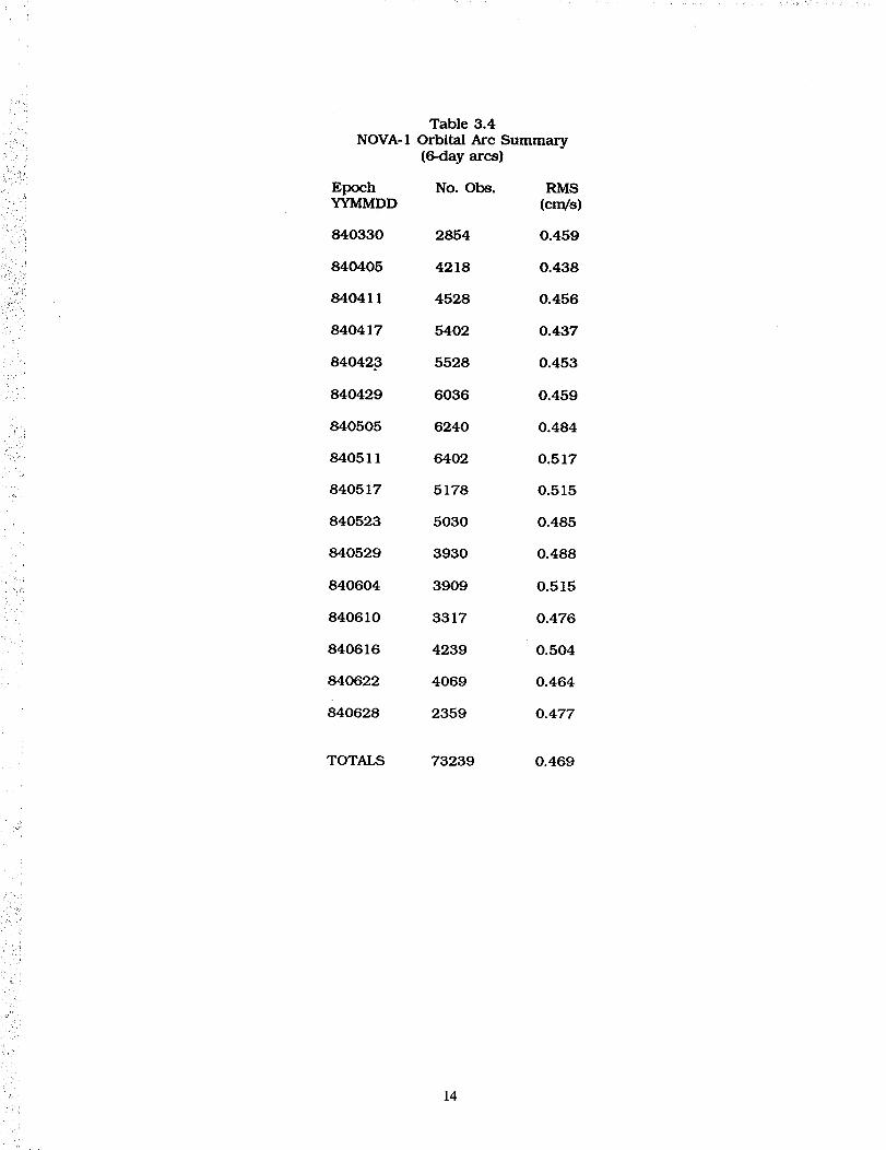
Table 3.4

NOVA-I Orbital Are Summary_, , (6-day arcs)

Epoch No. Obs. RMSi! __i YYMMDD (era/s)

' 840330 2854 0.459

_ ::_ 840405 4218 0.438

,_i 840411 4528 0.456

i_ i 840417 5402 0.437

. 840423 5528 0.453

840429 6036 0.459

_ii 840505 6240 0.484

840511 6402 0.517

840517 5178 0.515

840523 5030 0.485

840529 3930 0.488

_i I

:' 'i 840604 3909 0.515

_i 840610 3317 0.476

840616 4239 0.504

840622 4069 0.464

840628 2359 0.477

TOTALS 73239 0.469

• i__

14

Table 3.3

:_!:: Ajisal Orbital Arc Summary

_:_ _ Epoch No. Obs. RMS No.: : (YYMMDD) (cm) Stations

860818 5859 31.2 I0823 3416 29.4 12

.....:_ 828 2197 18.8 I0_i_:!i_ 901 5305 34.4 12

906 3803 22.8 12911 3281 22.6 12

860916 3471 21.2 II921 3663 27.7 9

ii!_:!_ 926 3003 24.9 9I001 3053 26.2 9

:i_:ii 1006 5480 21.6 I01011 3543 21.6 10

861016 3503 29.7 131021 3514 23.5 I01026 3039 24.4 I0II01 3280 26.4 II1106 3584 22.4 II1111 4306 21.0 12

861116 2538 18.7 II1121 4319 22.4 II1126 5425 23.1 111201 5605 25.5 111206 2854 24.0 91211 1678 21.8 6

!

861216 2876 24.4 81221 1208 23.9 71226 898 13.8 5

870106 6495 20.8 7III 7059 18.2 7116 4743 10.4 7

870121 4831 20.0 9126 9173 23.5 11201 7522 18.7 7206 6414 15.5 I0211 2705 10.4 8216 12558 17.8 9

.... 13

8L6I-gL6I s'4oea,l, ptmoIo g--SO_/D/9--SJN E'E o_ng!d

f O_

09

OL

2O8

i_iil Table 3.5i GEOS-3/ATS-6 ORBITAL ARC SUMMARY

SST LaserI

'" 'J ARC TIME NO. PASSES Rng-Rate Range_ START STOP SST Laser RMS NOBS RMS NOBS

YYMMDDHHMMSS (cm/s) (m)

_ :! 750425000000 750430000000 14 13 0.140 3007 0.441 445

:L: 750507000000 750508112320 3 5 0.134 590 0.228 129

750510000000 750514000000 9 13 0.104 1612 0.545 261

750518000000 750520194010 8 9 0.108 1549 0.727 298

750522000000 750526182500 16 I0 0.202 3069 0.311 219

750527000000 750531153850 15 13 0.174 3078 0.312 431

750617000000 750621000000 13 13 0.233 2116 0.452 444

ii 761219000000 761224033934 I0 18 0.251 2579 0.354 519

761226000000 761229164804 6 8 0.151 1474 0.420 363

770626000000 770630000000 2 19 0.073 223 0.644 772

770712000000 770716000000 2 8 0.077 173 0.423 378

770727000000 770731000000 5 17 0.177 568 0.658 795

770803000000 770807000000 6 18 0.116 534 0.961 783

770808000000 770812000000 5 25 0.137 691 0.745 1122

770813000000 770817000000 3 19 0.106 397 0.557 688

770818000000 770821000000 2 6 0.057 311 0.231 194

780921000000 780925000000 2 14 0.092 399 0.602 540

780926000000 781001170654 4 28 0.211 803 0.688 1287

:i! i.... : 781004000000 781008170424 4 21 0.168 882 0.660 802

781010000000 781014185044 2 37 0.050 382 0.700 1446

781018000000 781022000000 2 23 0.061 370 0.603 936

781025000000 781029215134 4 20 0.157 757 0.799 805

:: 781107000000 781112214700 4 22 0.200 734 0.696 732

790109000000 790116000000 2 23 0.049 409 1.551 955

790117000000 790121181500 3 18 0.047 353 1.626 863

790212000000 790216183454 2 17 0.050 338 0.650 820

i!

15

i

" satellite. The dominant portion of the range-rate signal is the inter-satellite range-rate between, :i: _ the geosynchronous satellite and the low orbiting satellite. The-ground-to-ATS-6 link in the:::_i measurement is made at S-Band frequencies while the inter-satellite link is made at C-Band.

Fortunately, this later link takes place above the atmosphere and only at the extremes involvingj : horizon tracking, does the inter-satellite signal penetrate the ionosphere. In such circumstances

(i.e., if the inter-satellite vector passes within 300 km of the Earth's surface) these data wereedited.

?,

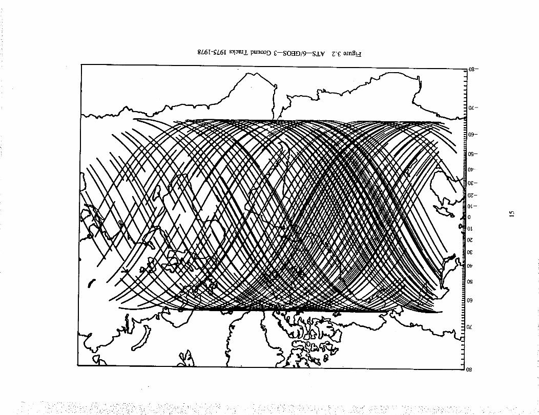
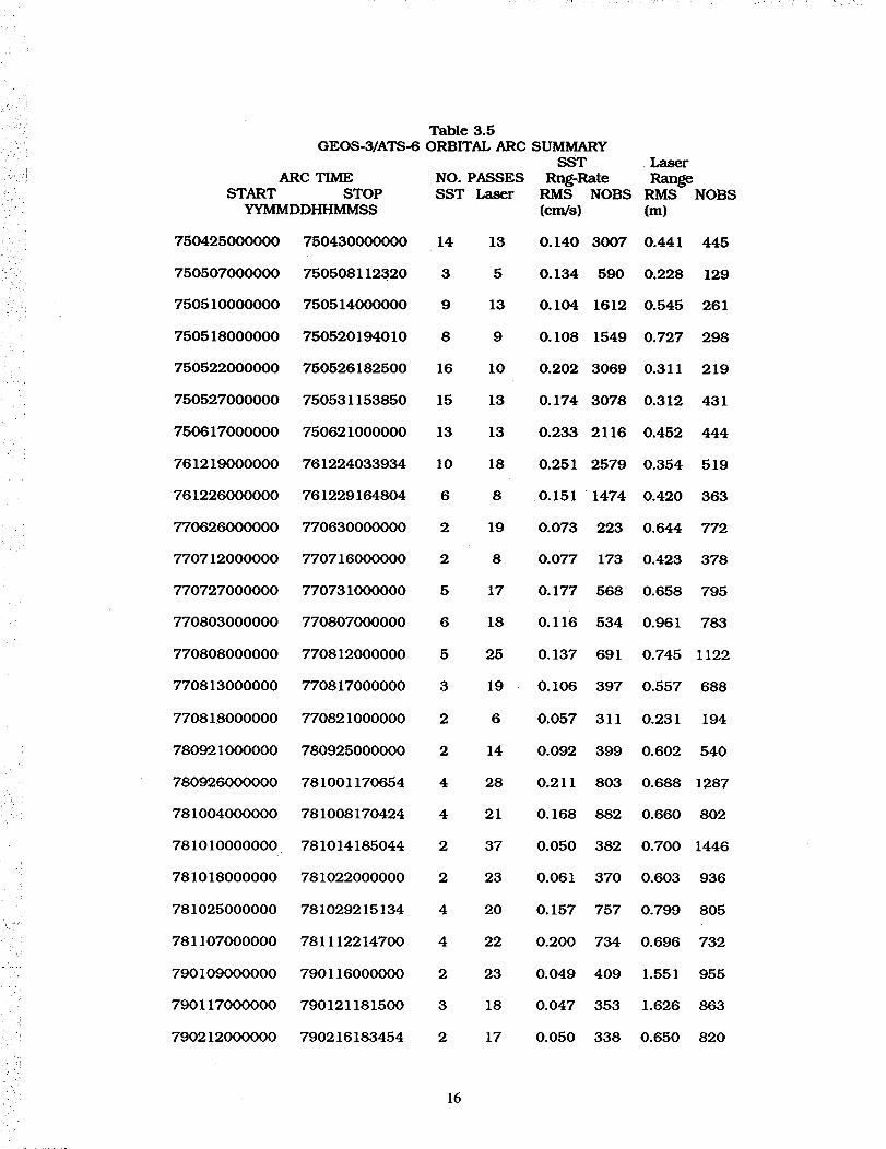
:,ii;i' The SST data available from GEOS-3/ATS-6 is presented in Figure 3.2. ATS-6 was atii_iii, 140°W longitude for most of the observations taken over the Pacific Ocean. The satellite was::_! moved to a position over Africa for the acquisition of the eastern hemisphere data. While ATS-_: :: 6 was in its drift phase between these locations, passes over South America and the Atlantic• Ocean were observed. Nearly two-thirds of these data -- 148 out of a possible 226 passes -- were

used (the others lacked suitable ground tracking support) for the 26 5-day arcs of SST utilizedin GEM-T2. This is the first time any of these data have been utilized within the GEM modeldevelopment. Table 3.5 summarizes these arcs and the initial observation statistics obtained in

forming the normal equations. GEM-TI was used as the apriori model for these computations.

3.4 Landsat-1 S-Band Radar Two-way and Three-way Average Range-Rate Observations

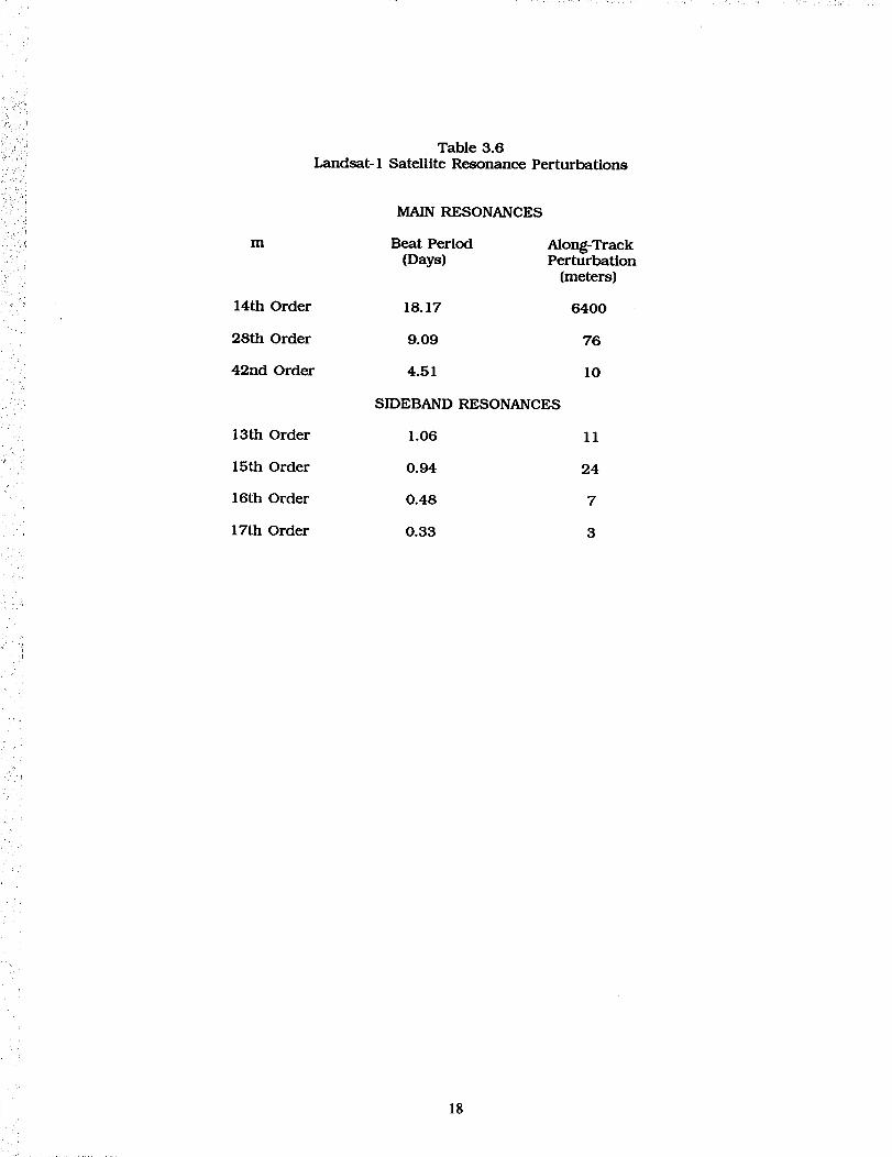
Landsat-1 is an Earth imaging satellite placed into a circular sun-synchronous orbit at analtitude of approximately 900 km. Being Earth imaging, Landsat required active attitudemaintenance throughout its entire mission. However, when the satellite was deactivated in 1974,two months of thrust-free data were acquired on this satellite to support geodetic modeling efforts.Landsat-1 observations are very important for geopotential field recovery for many satellites areplaced into orbit at this inclination for sun-synchronous mission requirements. SPOT-2, EOSand ERS-1 are future missions requiring precise orbits, and which are to be placed into orbitshaving very similar characteristics. Landsat-1 is also very interesting from a satellite geodesystandpoint given its very large, shallow resonance perturbations with the 14th, 28th and 42nd

order terms in the gravity spherical harmonic expansion. These resonance effects are given inTable 3.6 and represent some of the largest such effects seen within GEM-T2.

The Landsat data were acquired by the Unified S-Band Tracking Network which was theoperational network supporting NASA missions throughout the 1970's. Two-way (i.e., station tosatellite to station) average range-rate data were acquired by sites located at GSFC, Madrid(Spain), Guam, Goldstone (California), Ascension Island, Bermuda and Hawaii. Three-way datawere also acquired between several antennas located at GSFC and Goldstone where one station

transmitted while two widely separated stations received the satellite return signal. Unfortunately,these data lacked any correction for ionospheric refraction effects which for daytime passes duringhigh solar activity could produce measurement errors of 1 to 2 cm/s which is at the level of fitwe find for these observations. However, the data residuals were scrutinized and an elevationangle cutoff of 10 degrees was used (whereas these systems typically tracked to the horizon) toreduce problems resulting from this error source.

3.5 New Optical Data in GEM-T2

Table 3.7 summarizes the additional optical satellites which were added to GEM-T1 informing GEM-T2. Briefly stated therein is the reason these data were selected for the GEM-T2

solution. Figure 3.3 shows the SAO Baker-Nunn camera locations which provided the trackingfor these satellites whereas Table 3.8 shows the number of observations from each station

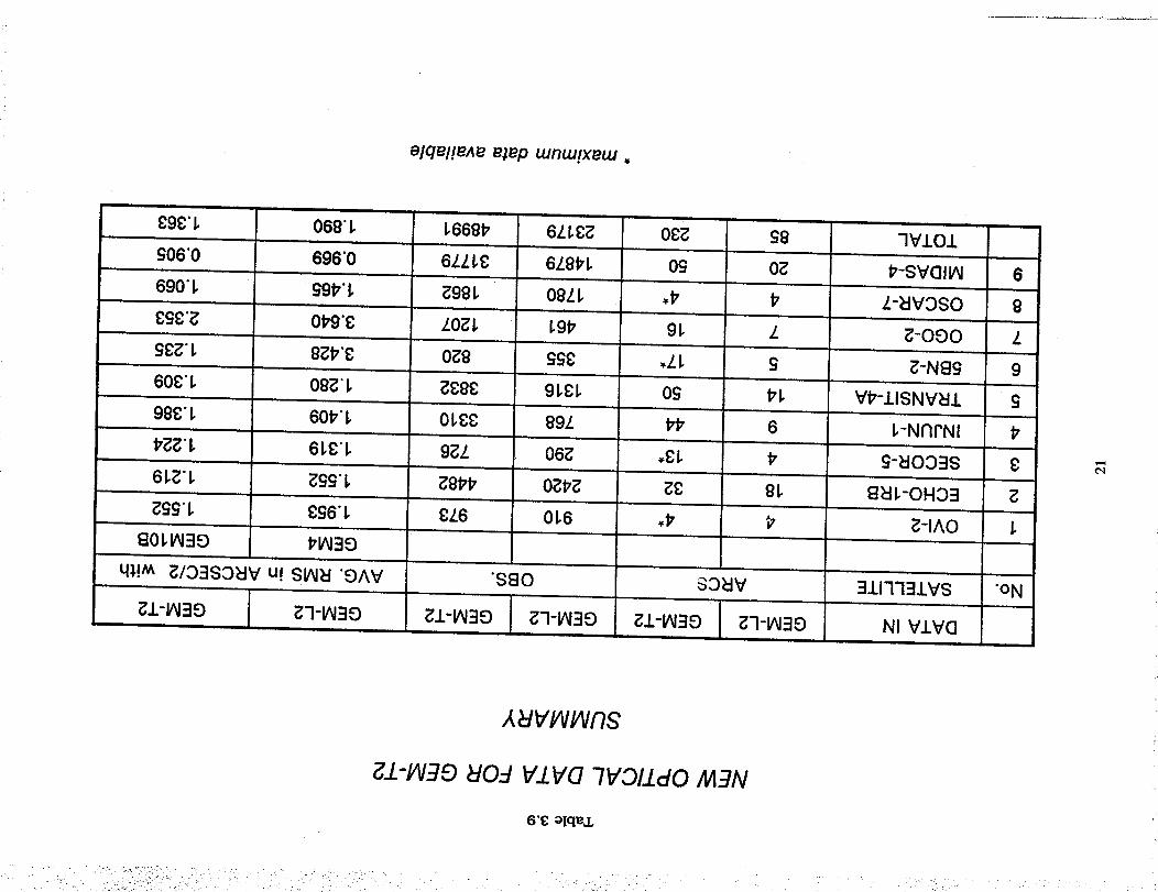
included in the field. The geographic distribution of the stations is good and all sites acquiredsignificant numbers of observations. Table 3.9 summarizes the number of 7-day ares and thenumber of observations utilized in GEM-T2. It also compares the current processing of theseobservations for inclusion in GEM-T2 versus that for GEM-7 in 1976 which was the last time

these data were reduced to form normal equations. Improved processing and apriori informationis evident. In total, 9 new optical data sets were added to GEM-T1 giving more than twice thenumber of these observations within the GEM-T2. Surprisingly, these data are important for thedefinition of the field, especially in the determination of the zonal and resonance orders in thegravity model.

: 17

' _ ' Table 3.6

:_: ! Landsat-I Satellite Resonance Perturbations

_i::"i MAIN RESONANCES

....._:,: m Beat Period Along-Track(Days) Perturbation

_ (meters)

_ 14th Order 18.17 6400

28th Order 9.09 76

42nd Order 4.51 10i i

SIDEBAND RESONANCES

13th Order 1.06 11

15th Order 0.94 24

16th Order 0.48 7

17th Order 0.33 3

18

.:i ¸¸,

k¸

_,_' Table 3.7

....,_::,_ NEW OPTICAL DATA FOR GEM-T2,P ,

i i:

No. SATELLITE INCLINATION MEAN MOTION REASON FOR SELECTIONDEGREE REV/DAY

1 OVl-2 144.27 11.45 Fill in inclination gap.

2 ECHO-1RB 47.21 12.21 Fill in inclination gap..l"

L

3 SECOR-5 69.22 11.79 Inclination near TOPEX.

_.; 4 INJUN 66.82 11.79 Inclination near TOPEX.i . . 1

5 TRANSIT-4A 66.82 13.85 Inclination near TOPEX.

6 5BN-2 89.95 13.46 Resonance close to TOPEX.7 OGO-2 87.37 13.79 Resonance close to TOPEX,.

8 OSCAR-7 89.70 13.60 Resonance close to TOPEX.

: 9 MIDAS-4 95.83 8.69 Unique resonance and inclination.

Table 3.8

DISTRIBUTION OF OBSERVATIONS FROM BAKER-NUNN STATIONS

f ,

SATELLITE SAO BAKER-NUNN STATIONS9001 9002 9003 9004 9005 9006 9007 9008 9009 9010 9011 9012

::i OVl-2 114 71 138 70 30 134 90 112 48 96 4 66ECHO-1RB 428 558 686 404 226 224 362 162 489 549 394SECOR-5 48 123 165 32 6 42 34 32 36 30 134 44

i INJUN-1 499 427 522 120 262 108 167 104 186 169 322 428TRANSIT-4A 595 546 787 246 267 54 134 116 146 196 310 435

5BN-2 150 74 58 44 16 104 20 62 54 76 58 104• OGO-2 135 154 115 98 36 87 102 54 32 81 86 156

OSCAR-7 63 118 246 80 380 194 102 94 34 186 365MIDAS-4 4056 843 766 2722 1306 2929 2550 2658 3146 2174 2243 2839

TOTAL 6088 2914 3483 3816 2149 3838 3515 3602 3904 3345 3892 4831

i

• ' 19

,o _-- |go,OOOOl

8 09006

20 - 0901_

09

0

40-

• PRINCIPAL SITES60-

801 I200 240 20o s2o o 40 so _2o _6o

Figure 3.3 SAO BAKER-NUNN Camera Stations

aiqel!RAe el_P wnuJ!xew.,

, |

g9g"1, 069"I, 1,6681;' 6/.1,8_ 08_ £8 7VIO.LJ

£06"0 696"0 6Z/.1,g 6/.8P1, 0£ O_ I;'-SV(311AI 6, • ,,,

690"1, £9P"!, _991, 08Z1, _,t7 t' /.-_:IVOSO 8i i

g£8"g 0l_9"8 /.0_1, 1,9t, 91, /. _-000 Z, ,,,, , , ,, ,, •

£g_"1, 8_P'g 0_9 ££g _,/.1, £ _-NI3£ 9

608"1, 08_"1, ;_888 91,81, 0cj 1;'1, V_-.i.ISNV_.L £

988"1, 60t'"1, 01,88 89/. 1;'17 6 1,-N17f'NI #

I;'_" 1, 61,8"1, 9;_Z 06;_ .81, # £-EIOO::IS 8

6I,_"I, ;_£cj"1, ;_8trP 0;_#;_ ;_8 81, BEi1,-OHO=l

_££"1, 8£6"1, 8/_6 01,6 ,,# # _-IAO 1,

801,W39 t,V_39

q_!,'_ g/O3S:3EIV u! SI/_EI"OAV "$80 S:3EIV 3117731V8 "ON

;_l-IAI30 g7-_30 ;_1-I/_30 ;_7-_30 _l-IAI30 _7-_30 NI VIVOi i

,4 V1411411"?S

I-IN=70 !09 V.LVQ -'lVOlldO /HEN

6"£ alqe3.

_f

? ]

i• /•,

'21::;_i

' SECTION 4. SOLUTION DESIGN:, ESTIMATION WITH OPTIMUM DATA WEIGHTING

.,.' ',

Our general method of weighted least squares with apriori signal constraints was. implemented for the estimation of the Goddard Earth Models in the late 1970's (Lerch et al.,i. 1979). This method has been modified in GEM-T2 to include a new optimum data weighting; ;' technique which automatically calibrates the errors for the estimated gravity field (Lerch, 1989).

, Some review is made herein of our general solution methodology. Our constrained least squares,: method is analogous to least squares collocation (Morltz,1980) and has permitted us to extend

_>,,:: the size of the adjusting model. The extension of the size of the solution to higher degree andorder allows us to more thoroughly exhaust the gravitational signal sensed by ever more precisetracking technologies. Stable solutions extending beyond 16x16 were possible using this method

' _ whereas correlation among high degree coefficients caused unreliable coemctent adjustments whenmodels were made lacking these constraints. As computer capabilities improved, satellite-onlymodels were extended to degree and order 36 (as In GEM-T1) and increased significantly to thepresent size of GEM-T2. This earlier method (which now has been extended to provide optimaldata weighting) is discussed in detail within Marsh et al., (1988) where it was shown to beanalogous to the work of Moritz (1980).

In our general estimation process of the GEM solutions the new weiglatlng technique hasbeen integrated into the solution design. The method determines the weights for the data subsetsacross the different satellite tracking systems on different orbits in order to automatically obtain

? an optimum least squares solution and an error calibration of the adjusted parameters. Theweighting system is designed to produce realistic error estimates. The data receive optimal

: weight in the solution according to their contribution to the model's accuracy. The methodemploys data subset solutions in comparison with the complete solution and uses an algorithmto adjust the data weights by requiring that the differences of the parameters between solutionsagree with their corresponding error estimates. With the adjusted weights, the process provides

/, for an automatic calibration of the solution's error estimates. The data weights which areobtained are generally much smaller than the weights associated with the accuracies of theobservations (noise-only) themselves.

.?

This algorithm is now an integral part of our general estimation technique. The weightingalgorithm has been applied to the least squares process of minimizing the weighted observation

' residuals with aprlorl constraints on the size of the signal obtained from the known power

; spectrum of the terrestrial gravity field. The main purpose of the apriori signal constraints is toprovide stability for the high degree terms, allowing the signal to be exhausted by the model.

_ The data weighting previously used in GEM-T1 and other earlier GEM models was basedon a series of tests using selected arcs of tracking data, independent gravity anomaly data, and

," orbital deep resonance predictions to test the characteristics, performance and sensitivity of< candidate fields. Models which were found to give better performance on these tests were studied,

and data weights were further refined until an optimal model was developed based upon thesecriteria. The new weighting system is an outgrowth of the process undertaken to evaluate in greatdetail, the accuracy of GEM-T1 (Lerch et al., 1989) and the overall means for calibrating modeluncertainties. The data weights selected for GEM-T1 have been specifically confirmed in these

i studies. However, when the complete data set for GEM-T2 Is assembled, even the weights for:_ GEM-TI's original data show some variation because of the increased data coverage In GEM-T2.

_ There are two major concerns in the proper weighting of least squares normal equations:

(a) weighting the individual observations corresponding to the expected accuracyof the observations within an aposterlorl context. Ideally, these are the so-called "noise-only"statistics; and

PRECEDING PAGE BLANK NOT FILMED 23 _ _;_ ....

i (b) accounting for the effects of unmodelled biases and forces on the solution byreweighting the normal equations to balance the solution for the non-uniform presence of theseeffects.

The normal least squares solution accounts for (a) but not for the effects of (b) without somespecial analysis and selection of an optimal data weighting algorithm.

i

:il. 'Within a least squares solution in the ideal case, the observation residuals approximatetheir noise-only distribution so that:

.... ((_r2/02)/num) = 1 (4.1)

=' where r is the observation residual, num is the number of observations and o corresponds to its_ noise-only observational uncertainty. This behavior is common in theory where observations are

unbiased, uncorrelated and where data noise is the dominant error source. However, theobservations available for gravitational field recovery and the ancillary force and measurementmodels which are required to isolate this gravitational signal depart markedly from this ideal ease.Our solution suffers from a great many sources of systematic error, imperfect environmental andmeasurement models, neglected small force modeling effects and a host of other problems whichneed to be addressed if an optimal gravitational modeling solution is to result. Ourunderstanding of these problems is presently limited to approximate estimates of the errormagnitudes in our models, and we unfortunately lack the observations and the resources toimprove everything which is part of our solution environment. The net result is that our solutionaposteriori can only fit our most precise data sets, such as the observations provided by advancedlaser systems, to a factor of 3 to 10 worse than their noise-only expectation of systemperformance. These problems cause optimization of data weighting and field calibration to bemajor undertakings if an improved solution with well understood and reliable error estimates isto result. Unfortunately, data noise has only a modest impact on the final data weights which are

• • obtained., i

Satellite orbital characteristics, area-to-mass ratios and the number/deployment ofcomponents comprising the satellite bus etc. are highly variable, which causes some satellites toexperience much larger and more difficult to model non-conservative force model effects.Atmospheric drag for lower altitude satellites presents a serious modeling problem with presentstate-of-the-art atmospheric density models yielding errors of 20 to 30% for satellites atgeodetically useful orbits of 800 to 1200 km altitude (Hedin, 1988). Adjustment of empiricalcoefficients scales the effective atmospheric density given by the drag models through a scalingof the drag acceleration over some temporal interval in an averaged sense. However, thesecoefficients do little to ameliorate problems associated with the nature and detailed structure ofthe fluctuations in density which exist but are presently unmodeled by contemporary densitymodels within these averaging intervals. Drag is by no means unique in its imperfectrepresentation.

The aposteriori RMS of fit to the observations gives some measure for determining theeffective data weights by reflecting, in a relative sense, these force model difficulties especiallywhen common tracking systems are used to acquire data on different orbits. Obviously, thisrelative comparison cannot be applied uniformly since few satellites are tracked by more than onetracking technology, and the tracking systems evolve over time. Nevertheless, the relative RMSof fit achieved from the solution is still used. However, assessment made across data sets can

only be approximated and is based on some broad characterization of system noise-onlycharacteristics when determining relative data weights.

However, when these systematic errors are present, they do not manifest themselves asrandom data residuals. This non-randomness (strongly seen within a pass of observationresiduals) must also be accommodated through data reweighting. Furthermore, this requirestaking into account the number of points in a typical pass of data so affected. This reweightingWj, must be optimized across all data subsets J, which are used in combination to form the

24

combined solution normal-equations whose inversion yields the gravitational solution. Wj asderived in Lerch, (1989) can be shown to approximate:

' i

:':'; (Nobsj)(RMSj)2(4.2)

where: (Since the assigned aprlori data noise uncertainty should represent the true noise in the: data although this is seldom the case, an additional adjustment to the data weights is commonly

_ needed.) RMS! is the aposterlorl rms of fit to the observation subset J, and Nobsj is a valuecorrespondin_ to a typical number of points in a pass of tracking data. In practice, the RMS! isscaled by a factor which changes with differing tracking technologies. Hence 8t indicates theerror showing the true value of a single observation of type J on the solution (see'Tables 4.1 and4.2).

The method for the solution requires the minimization of the sum Q which is ai combination of signal and noise as follows:

C2[, m + S2I, m

O =_ ................... -F _ Wj rj 2o21

(4.3)

where the signal is given by

CI,m and SI, m : which are the spherical harmonics composing the solution coefficients;.... and

a I : is a modified version of Kaula's rule which is the known power of theterrestrial gravitational field.

The noise is given by:

rj : which are the observation residuals of the respective tracking system; and

"•' Wj : which is the optimal weighting factor which compensates for unmodelederror effects (which should ideally equal the reciprocal variance of the noiseof the respective tracking system).

When minimizing Q using the least squares method, the normal metric equation and errorcovariance is obtained as follows:

Wl Nj x = Wl R1 are the original normal equations for the jth data subset (seeLerch, 1989).

:_ The solution is formed after summing each of the satellite data normal matrices Nj overthe entire range of data subsets giving a combined normal matrix for the solution by:

N = K "1 + _ % Nj (4.4)

25

The:

ii i

i.? C21m + S21m,.:: K = _ ..............

o21(4.51

!: ..... matrix is the diagonal signal matrix which is introduced to achieve improved stability for thegravitational model adjustment. This modified least squares method stabilizes the solution

: through the minimization of the size of the adjusting gravitational terms above a certain degreecutoff.

Letting j =0 denote the least squares subset normals for the apriori signal constraints forthe coefficients, K (as in 4.5), then the complete normals for minimizing Q in (4.31 is given by:

i "

7N x = R (4.61

where

N--_ WjNj1=0

: wjRj: j=o

: and

Vxx = N"1 Is the approximate form for the error covarlance matrixwhich should yield reliable parameter uncertainties if proper

weighting factors (Wj) are used.

The weight W 0 signifies the scale for the aprlorl signal constraints on the static gravityparameters. It is held fixed at unity since the power spectrum of the gravity field is well known.

On the other hand, the optimal weights Wj for the satellite tracking data are quite variable asshown in Tables 4.1 and 4.2, _md can depart from the nominal noise-only values by up to two

; orders of magnitude. Clearly, it is these weights which must be determined and optimized. Weview the automation of this process as a considerable advancement.

4.1 The Optimal Weighting Algorithm

• The automatic data weighting algorithm as developed by Lerch (19891 is given by the. following procedure:

Let the normals for data set t be defined as (w - W):

:_ wtN t = w tR t (4.7}

i .

26

where N is the normal matrix for data set t, R is the normal matrix of observation residuals, andw t is the weight in the iterative solution. The complete solution containing all data sets is givenas:

x = ( _ wjNj)_(_wjRj)j (4.8)

A subset solution which lacks data set t is given as:

xt = (_ %Nj)'1(_wjRj)j_t j_t

(4.9)

The covariances for solution x and x t are respectively:

V(x) = (_ wjNj)'I and V(x t) = (_ wj Nj)"1j j_t

(4.10)

The normal residuals for these solutions are:

R(x) = (X wjRj) and R(x t) = (X wjRj)j j_t

(4.11)

The difference between the subset and full solutions can be predicted by their respectivecovarianees. This is the principle behind this calibration and determination of optimal dataweighting technique. The difference between the two fields reflects the unmodeled errors in dataset t, since the error effects to first order, subtract out for the data sets common to bothsolutions. The difference is simply:

x t - x = V(x t) R(x t) - V(x) R(x)(4.12)

If E is used to express the expected value, then the differences in these models are predicted bythe error covariances of the solution differences given by:

E( x t - x)(x t x) T = V(x t) - V(x)

= V( xt - x)(4.13)

27

We can now introduce the calibration factor k t for the t data subset which is being: computed. If the trace of a matrix is denoted as TR and we restrict the analysis to only the gravity

: i coefficients, then k t is given as:

:' _,:i ( xt- x)T (xt- x) = ktTR [V(x t - x)]',_",i (4.14)

_i_ii__ and the adjusted weight as:

"Wt* _-- wt/k t

" (4.15)

_ Since the subset and complete solution alike change when the weight on a subset data set is_i__':,! altered, these weights require iteration. Several successive solutions are produced using improved_ weights until the calibration factor, k t, equals 1 for each data subset. Quite remarkably, the

...... weights converge in only a few iterations, as shown later in Table 6.1. Moreover, these calibratediweights largely follow the estimate based on the aposteriori RMS of fit and number of points ina typical pass as shown in equation (4.2).

Tables 4. la and 4. lb present the major data subsets comprising GEM-T2. Also shown isthe aposteriori RMS of fit (approximate) of the observations and the final weights computed. The

computation of the weights and the automatic error calibration which results is discussedthoroughly in Section 6.

Table 4.1a

•SATELLITE DATA IN GEM-T1SIGHA*

SEMI MAJOR INCL DATA # OF X OF RESID. WEIGHTS^

SATELLITE AXIS (km.| ECC DEG TYPE ARCS OBS o c oc

1 LAOEOS 12273. .0038 109.85 LASER 57 1_4527 10_m. 112cm.

2 STARLETTE 7331. .0204 49.80 LASER 46 57356 20cm. 224cm.

3 GEOS-3 7226. .0008 114.98 LASER 36 42407 70cm. 816cm.

4 PEOLE 7006. .0164 15.01 LASER 6 4113 90cm. 816cm.

5 BE-C 7507. .0257 41.19 LASER 39 64240 50cm. 577cm.

CAMERA 50 7501 2 ar©sec 5.6 arcsec

6 GEOS-1 8075. .0719 59.39 LASER 48 71287 70cm. 667cm.

CAMERA 43 60750 1 ircse¢ 8.9 arcsec

7 GEOS-2 7711. .0330 105.79 LASER 28 26613 80©m. 816cm.

CAI4ERA 46 61403 1 arcse¢ 8.9 arcsec

8 Dl-C 73_1. .0532 39.97 LASER 4 7455 150cm. 816cm.

CAMERA 10 2712 2 arcsec 7.3 arcsec

9 01-0 7622. .0848 39.46 LASER 6 11487 100cm. 816cm.

CAMERA 9 6111 2 arcsec 8.9 arcsec

10 SEASAT 7170. .0021 108.02 LASER 14 14923 70cm. 707cm.

DOPPLER 14 1380_2 .Scm/sec 7cm/sec

11 OSCAR-14 7_40. .0029 89.27 DOPPLER 13 63098 lcm/sec 8cm/sec

12 ANNA-1B 7501. .0082 50.12 CAMERA 30 4463 2 arcsec 4.5 arcsec

13 BE-B 7354. .0135 79.69 G/U4ERA 20 1739 2 ircsec 4.5 arcsec

14 COURIER-18 7469. .0161 28.31 CAMERA 10 2476 2 ercsec 4.5 arcsec

15 TELSTAR-1 9669. .2429 44.79 CANERA 30 3962 2 Ircsec 4.5 arcsec

16 VANGUARD-2RE 8496. .1832 32.92 CAMERA 10 686 2 $rcsec k.5 arcsec

17 VAHGUARO-2 6298. .1641 32.89 CAMERA 10 1299 2 srcsec 4.5 srcsec

1

* SIGMA(_) =(_)2

29

...." Table4.IB' i

NEW SATELLITEDATA IN GEM-T2 IN ADDITION TO GEM-T1

:_ SEMI MAJOR INCL DATA # OF # OF RVIS SIGMA; : ._,_._LT.ELLLT_AXIS t'km,) I.:::CC DEG. TYPE ARCS OBS. RESID. WEIGHTS

° t 8tLAGEOS 12273 .0038 109.85 LASER 29 134093 10om. 1120m.

'84,'85,'86,'87

STARLETTE 7331 .024 49.80 LASER 38 40041 20cm. 224cm.'83,'84

STARLETTE LASER 73 411102 20cm. 500cm!:_ '86

_ AJISAI 7870 .0006 50.0 LASER 36 156021 16cm. 316cm.

GEOS-1 °80 8075 .0719 59.39 LASER 30 54129 32cm. 258cm.

GEOS-3 '80 7226 .0008 114.98 LASER 50 54526 25cm. 224cm.

GEOS-3 LASER 26 17027 70cm. 816cm.GEOS-3:ATS 41867 .001 0.9 SST 9 19074 .4cm/sec 7.1cnVsec

'75,'76GEOS-3:ATS SST 17 8326 .2cm/sec 3.2cm/sec'77,'78,'79

NOVA 7559 .0011 89.96 _ 16 73238 .4cm/sec 2.6cm/sec

LANDSAT-1 7286 .0012 99.12 _ 10 26426 1.5cm/sec10.5cmlsec

GEOSAT 7169 .0008 108.0 DOPPLER 13 549141 1.3cm/sec 4.5cm/sec

OVI-2 8317 .0184 144.27 CAIVERA 4 973 2 arcsec 5.8 arcsec

ECHO-1RB 7966 .0118 47.21 CAt_RA 32 4482 2 arcsec 8.2 arcsec

SECOR-5 8151 .0793 69.22 C_ 13 726 2 arcsec 5.8 arcsec

INJUN-1 7316 .0079 66.82 CAMERA 44 3310 2 arcsec 8.2 arcsec

TRANSIT-4A 7322 .0076 66.82 CAMERA 50 3832 2 arcsec 8.2 arcsec

5BN-2 7462 .0058 89.95 CAIVERA 1 7 820 2 arcsec 8.2 arcsec

OGO-2 7341 .0752 87.37 CAMERA 1 6 1207 2 arcsec 8.2 arcsec

OSCAR-7 7411 .0224 89.70 CAtvERA 4 1862 2 arcsec 5.8 arcsec

MIDAS-4 9995 .0112 95.83 CAMERA 50 31779 2 arcsec 8.2 arcsec

: 30

i>

SECTION 5. THE GEM-T2 GRAVITATIONAL MODELING SOLUTION RESULTS

i :: i This section discusses the major products of the GEM-T2 solution which include:

O the static gravitational model,

O an expanded model for selected long wavelength ocean tidal terms,

_: O station coordinates for the 45 TRANET sites tracking GEOSAT, and

O the Earth polar motion and orientation series.i!

Where applicable, these models and their uncertainty estimates will be compared with othersolutions to provide a qualitative understanding of the accuracy of these results.

. 5.1 The GEM-T2 Gravitational Solution

Table 5. I presents the normalized spherical harmonic coemcients for GEM-T2. These

coefficients describe the static geopotential in classical spherical harmonic form given by:

GM f Imax l

U = [ I + _ _ (ae/r)l Pl,m (sin_b)*r I=2 m=0

( CI,m cos ITIA-b Sl, m sin m A ) lJ (5.1)

where:

G is the gravitational constant,M is the mass of the Earth,_b is the satellite geocentric latitude,k is the satellite cast longitude,Plm is the normalized associated Legendre function of the first kind; andClm,Slm are the normalized geopotential coemcients.

The geopotential forces are computed as the gradient of the potential U. The calibration of themodel uncertainties are discussed in Section 6.

•5.2 The GEM-T2 Ocean Tidal Solution

The GEM-T2 solution solves for temporal changes in the external gravitational attraction: of the Earth sensed by near-Earth orbiting objects at the major astronomical frequencies. These

tidal terms are not exactly equivalent with those measured on the ocean surface although they canbe similar in magnitude and of a comparable physical origin. Even when tides themselves arebeing sensed, a satellite experiences an attenuated signal from the solid Earth/oceans/atmospherewhich is a combined effect. An artificial satellite senses the mass redistribution associated with

the tides, but the tracking data taken on these objects has no way of discriminating between thetidal effects caused by deformation within the solid Earth apart from the oceans. We choose tosolve for terms in the space of ocean tides using a classical spherical harmonic representationas described in Christodoulidis et al., (1988), but this is merely a matter of convenience and notone of necessity. This approach is chosen since we believe that contemporary models of thefrequency-dependent solid Earth tidal response (Wahr, 1981) are better known at the-

i 31i

Table 5.1

GEM-T2 NORMALIZED COEFFICIENTS

UNITS OF 10sZONALS

INDEX VALUE INDEX VALUE INDEX VALUE INDEX VALUE INDEX VALUEN M N M N M N M N M

2 0 -484.1652998 3 0 0.9570331 4 0 0.5399078 5 0 0.0686883 6 0 -0.14960927 0 0.0900847 8 0 0.0483835 9 0 0.0284403 10 0 0.0549673 11 0 -0.0519374

12 0 0.0340918 13 0 0.0429873 14 0 -0.0208746 15 0 0.0008078 16 0 -0.006967417 0 0.0211398 18 0 0.0086686 19 0 -0.0048120 20 0 0.0199685 21 0 0.009575422 0 -0.0101581 23 0 -0.0241859 24 0 0.0010847 25 0 0.0069648 26 0 0.000948427 0 0.0027591 28 0 -0.0064182 29 0 -0,0008836 30 0 -0.0009634 31 0 0.007619332 0 -0.0027771 33 0 0.0051093 34 0 -0.0057588 35 0 0.0078141 36 0 -0.004791837 0 0.0022441 38 0 0.0013147 39 0 -0.0010497 40 0 0.0020610 41 0 0.001105142 0 0.0013010 43 0 0.0021499 44 0 0.0002269 45 0 0.0020158 46 0 -0.000821647 0 0.0008891 48 0 -0.0002987 49 0 0.0000776 50 0 0.0002472

SECTORIALS AND TESSERALS

INDEX VALUE INDEX VALUE INDEX VALUEN M C S N M C S N M C S

2 2 2.4390067 -1.4000870

3 1 2.0307524 0.2496027 3 2 0.9035391 -0.6189858 3 3 0.7215073 1.4137252

4 1 -0.5352557 -0.4741332 4 2 0.3482596 0.6640236 4 3 0.9913108 -0.20142884 4 -0.1893677 0.3089680

5 1 -0.0607595 -0.0950258 5 2 0.6560800 -0.3241298 5 3 -0.4518505 -0.21707115 4 -0.2950497 0.0513561 5 5 0.1719075 -0.6690593

6 1 -0.0771405 0.0253197 6 2 0.0524466 -0.3752434 6 3 0.0584154 0.00687826 4 -0.0868267 -0.4711255 6 5 -0,2660832 -0.5368830 6 6 0.0096978 -0.2369657

7 1 0.2818503 0.0962266 7 2 0.3209757 0.0956941 7 3 0,2523951 -0,20959987 4 -0.2742482 -0.1241968 7 5 -0.0001020 0.0196942 7 6 -0.3585523 0.15158787 7 -0.0014862 0.0252823

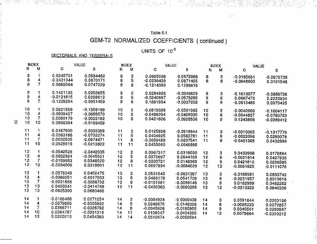
Table 5.1

GEM-T2 NORMALIZED COEFFICIENTS (continued)

UNITS OF 10.6SECTORIALS AN_ TESSERALS

INDEX VALUE INDEX VALUE INDEX VALUEN M C S N M C S N M C S

8 1 0.0245721 0.0584482 8 2 0.0695068 0.0672988 8 3 -0.0165651 -0.08707358 4 -0.2431044 0.0670171 8 5 -0.0236439 0.0871455 8 6 -0.0648602 0.31015488 7 0.0689064 0.0747229 8 8 -0.1214399 0.1206619

9 1 0.1421125 0.0253655 9 2 0.0284926 -0.0349829 9 3 -0.1613077 -0.08567369 4 -0.0121815 0.0258612 9 5 -0.0240867 -0.0575285 9 6 0.0667472 0.22336349 7 -0.1229254 -0.0951409 9 8 0.1881954 -0.0037058 9 9 -0.0613486 0.0970425

10 1 0.0831559 -0.1356199 10 2 -0.0819359 -0.0501065 10 3 -0.0040960 -0.160411710 4 -0.0939427 -0.0688070 10 5 -0.0489204 -0.0458035 10 6 -0.0344837 -0.078375310 7 0.0090179 -0.0022192 10 8 0.0421606 -0.0928536 10 9 0.1243856 -0.038941210 10 0.0966394 -0.0189409

11 1 0.0187900 -0.0302389 11 2 0.0125806 -0.0919944 11 3 -0.0310305 -0.131777911 4 -0.0363188 -0.0702274 11 5 0.0404925 0.0583781 11 6 -0.0022096 0.028007611 7 0.0032535 -0.0874471 11 8 -0.0059489 0.0237541 11 9 -0.0401308 0.043269611 10 -0.0529919 -0.0213622 11 11 0.0455060 ,0.0645895

12 1 -0.0542526 -0.0442035 12 2 0.0067317 0.0318030 12 3 0.0403968 0.017586412 4 -0.0632924 -0.0045521 12 5 0.0372697 0.0044109 12 6 -0.0021614 0.042793612 7 -0.0159953 0.0348520 12 8 -0.0233721 0.0148369 12 9 0.0421812 0.023658512 10 -0.0084006 0.0319901 12 11 0.0097894 -0.0084029 12 12 -0.0051825 -0.0111076

13 1 -0.0578349 0.0450475 13 2 0.0531545 -0.0631397 13 3 -0.0168961 0.083374313 4 -0.0089251 -0.0017503 13 5 0.0486179 0.0541729 13 6 -0.0231957 0.001061613 7 -0.0031866 -0.0056732 13 8 -0.0101581 -0.0099146 13 9 0.0182999 0.046225213 10 0.0400341 -0.0414749 13 11 -0.0430363 -0.0000298 13 12 -0.0310323 0.084030913 13 -0.0625300 0.0680460

14 1 -0.0165468 0.0271254 14 2 -0.0384924 -0.0000438 14 3 0.0391644 0.020310614 4 -0.0079895 -0.0005932 14 5 0.0245675 .0.0148326 14 6 -0.0095223 0.007285714 7 0.0366711 -0.0026792 14 8 -0.0345926 -0.0190955 14 9 0.0345501 0.029056714 10 0.0364787 -0.0031316 14 11 0.0138047 -0.0404306 14 12 0.0078664 -0.032021214 13 0.0320213 0.0454383 14 14 -0.0512674 -0.0050594

Table 5.1

GEM-T2 NORMALIZED COEFFICIENTS (continued)

UNITSOF 10.6SECTORIALS AND TESSERALS

INDEX VALUE INDEX VALUE INDEX VALUEN M C S N M C S N M C S

15 1 0.0122177 0.0111280 15 2 -0.0251562 -0.0288124 15 3 0.0401686 0.026259715 4 -0.0435169 0.0075971 15 5 0.0100013 0.0175705 15 6 0.0256916 -0.051539915 7 0.0607753 0.0152877 15 8 -0.0331076 0.0235607 15 9 0.0113370 0.044530115 10 0.0090273 0.0113802 15 11 0.0021578 0.0233866 15 12 -0.0321733 0.008724615 13 -0.0290699 -0.0041930 15 14 0.0067593 -0.0247259 15 15 -0.0189824 -0.0057180

16 1 0.0297624 0.0240565 16 2 -0.0140907 0.0248689 16 3 -0.0326144 -0.043991616 4 0.0396039 0.0473846 16 5 -0.0067956 0.0018428 16 6 0.0063436 -0.028497516 7 -0.0009530 -0.0126372 16 8 -0.0182064 0.0030949 16 9 -0.0188186 -0.038217116 10 -0.0127558 0.0083994 16 11 0.0183569 -0.0043302 16 12 0.0200031 0.005341716 13 0.0134693 0.0011027 16 14 -0.0194970 -0.0386309 16 15 -0.0161367 -0.031045016 16 -0.0341988 -0.0064019

17 1 -0.0286816 -0.0293496 17 2 -0.0042782 0.0141925 17 3 0.0119428 0.009326617 4 0.0116340 0.0224278 17 5 -0.0147210 -0.0050012 17 6 0.0050910 -0.017773117 7 0.0190439 -0.0103587 17 8 0.0393184 0.0073649 17 9 -0.0011019 -0.034798417 10 -0.0052074 0.0155743 17 11 -0.0123774 0.0154974 17 12 0.0296813 0.012986117 13 0.0170527 0.0208044 17 14 -0.0131460 0.0114902 17 15 0.0052124 0.005414317 16 -0.0315737 0.0022165 17 17 -0.0366559 -0.0215735

18 1 0.0020036 -0.0353441 18 2 0.0019658 0.0217675 18 3 -0.0026138 -0.005075318 4 0.0485785 0.0015282 18 5 0.0049920 0.0224950 18 6 0.0250848 -0.007257918 7 -0.0025170 0.0086473 18 8 0.0375154 -0.0047905 18 9 -0.0150018 0.030465118 10 0.0020478 -0.0109039 18 11 -0.0093050 0.0031534 i 8 12 -0.0271222 -0.018672518 13 -0.0063145 -0.0350284 18 14 -0.0089800 -0.0124657 18 15 -0.0417201 -0.018162818 16 0.0082039 0.0032907 18 17 0.0048942 0.0043880 18 18 -0,0003413 -0.0084223

19 1 -0.0132130 0.0009653 19 2 0.0072922 -0.0039028 19 3 -0.0027786 0.012157319 4 0.0047233 0.0075195 19 5 -0.0021981 0.0316768 19 6 -0.0069907 0.006687719 7 0.0032117 0.0075083 19 8 0.0266181 -0.0142467 19 9 0.0034732 0.016727419 10 -0.0364663 -0.0085933 19 11 0.0203631 0.0120152 19 12 -0.0024038 -0.000644119 13 -0.0060661 -0.0282432 19 14 -0.0045298 -0.0130308 19 15 -0.0172043 -0.012754519 16 -0.0219716 -0.0091235 19 17 0.0296710 -0.0134720 19 18 0.0301456 -0.007173919 19 0.0061595 0.0018905

Table 5.1

GEM-T2 NORMALIZED COEFFICIENTS (continued)

UNITS OF 10-8SECTORIALS AND TESSERAL$

INDEX VALUE INDEX VALUE INDEX VALUEN M C S N M C S N M C S

20 1 0.0157399 -0.0100026 20 2 0.0187443 0.0073043 20 3 0.0060908 0.017314420 4 0.0030529 -0.0036520 20 5 -0.0108465 0.0030199 20 6 0.0079275 0.006147120 7 -0.0118532 -0.0003759 20 8 -0.0056161 0.0006536 20 9 0.0237362 0.010847520 10 -0.0282901 -0.0114400 20 11 0.0155253 -0.0213370 20 12 -0.0061237 0.015782420 13 0.0276079 0.0059426 20 14 0.0110712 -0.0137433 20 15 -0.0267134 0.001551820 16 -0.0153321 -0.0020238 20 17 0.0067026 -0.0133355 20 18 0.0127771 -0.000231520 19 -0.0122968 0.0094362 20 20 0.0065287 -0,0031206

21 1 -0.0129057 0.0405056 21 2 0.0046612 0.0044867 21 3 0.0022573 0.022842321 4 -0.0044913 0.0116340 21 5 0.0118863 -0.0035430 21 6 -0.0072367 0.0019953

_ 21 7 -0.0123222 0.0001135 21 8 -0.0149498 0.0041740 21 9 0.0213432 -0.001764621 10 -0.0070501 -0.0018894 21 11 0.0139045 -0.0350282 21 12 -0.0027053 0.011322321 13 -0.0174796 0.0131394 21 14 0.0196161 0.0094325 21 15 0.0178718 0.013623621 16 0.0080497 -0.0076515 21 17 -0.0069162 -0.0022420 21 18 0.0232517 -0.008806921 19 -0.0238225 0.0135908 21 20 -0.0200855 0.0198500 21 21 0.0075325 -0.0082327

22 1 0.0099264 -0.0007388 22 2 -0.0200252 0.0082418 22 3 0.0071928 -0.005821022 4 -0.0101392 0.0105595 22 5 0.0035063 0.0014637 22 6 0.0091120 0.006654722 7 0.0101694 -0.0002510 22 8 -0.0095379 -0.0090097 22 9 0.0166858 -0.007771022 10 0.0022397 0.0178636 22 11 -0.0050223 -0.0130492 22 12 0.0067411 -0.010705322 13 -0.0168282 0.0196012 22 14 0.0094908 0.0081424 22 15 0.0250399 0.006075822 16 -0.0030291 -0.0080446 22 17 0.0115363 -0.0156888 22 18 0.0069583 -0.012320522 19 0.0066686 -0.0055346 22 20 -0.0160290 0.0213725 22 21 -0.0180893 0.018931522 22 -0.0029881 0.0063133 _

23 1 0.0037148 0.0123740 23 2 -0.0031104 0.0012627 23 3 -0.0101724 -0.006282623 4 -0.0155617 0.0035853 23 5 -0.0052477 -0.0015027 23 6 0.0015575 0.013956123 7 -0.0031648 -0.0021497 23 8 0.0039870 -0.0038722 23 9 -0.0047139 -0.004994623 10 0.0145802 -0.0073488 23 11 0.0107774 0.0175629 23 12 0.0171677 -0.023524023 13 -0.0107830 -0.0055874 23 14 0.0049840 -0.0041804 23 15 0.0178661 -0.002498423 16 0.0077297 0.0116023 23 17 -0.0047031 -0.0093385 23 18 0.0038581 -0.013057123 19 -0.0071011 0.0098609 23 20 0.0133809 -0.0056003 23 21 0.0125823 0.009577323 22 -0.0071855 -0.0041004 23 23 -0.0052198 -0.0055011

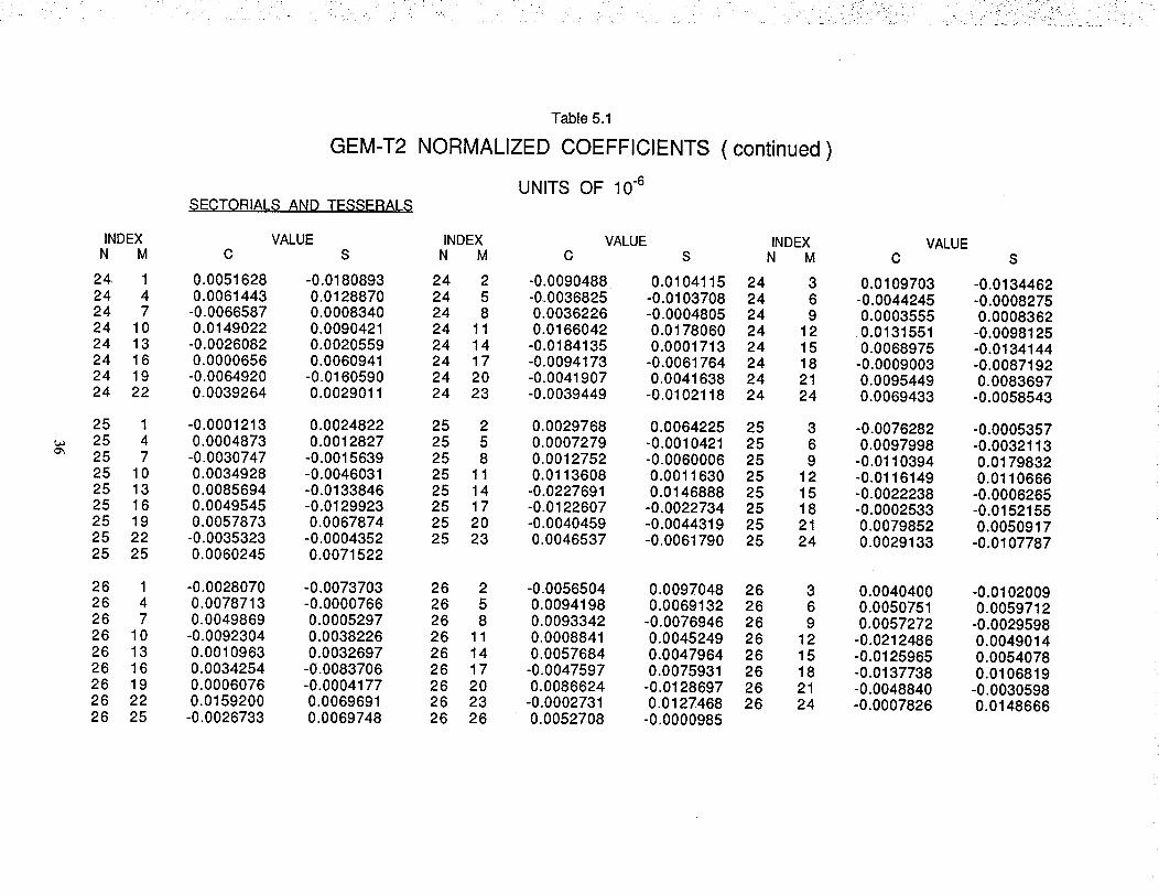
Table 5.1

GEM-T2 NORMALIZED COEFFICIENTS (continued)

UNITS OF 10 .6SECTORIALS AND TESSERAL$

INDEX VALUE INDEX VALUE INDEX VALUEN M C S N M C S N M C S

24 1 0.0051628 -0.0180893 24 2 -0.0090488 0.0104115 24 3 0.0109703 -0.013446224 4 0.0061443 0.0128870 24 5 -0.0036825 -0.0103708 24 6 -0.0044245 -0.000827524 7 -0.0066587 0.0008340 24 8 0.0036226 -0.0004805 24 9 0.0003555 0.000836224 10 0.0149022 0.0090421 24 11 0.0166042 0.0178060 24 12 0.0131551 -0.009812524 13 -0.0026082 0.0020559 24 14 -0.0184135 0.0001713 24 15 0.0068975 -0.013414424 16 0.0000656 0.0060941 24 17 -0.0094173 -0.0061764 24 18 -0.0009003 -0.008719224 19 -0.0064920 -0.0160590 24 20 -0.0041907 0.0041638 24 21 0.0095449 0.008369724 22 0.0039264 0.0029011 24 23 -0.0039449 -0.0102118 24 24 0.0069433 -0.0058543

25 1 -0.0001213 0.0024822 25 2 0.0029768 0.0064225 25 3 -0.0076282 -0.000535725 4 0.0004873 0.0012827 25 5 0.0007279 -0.0010421 25 6 0.0097998 -0.003211325 7 -0.0030747 -0.0015639 25 8 0.0012752 -0.0060006 25 9 -0.0110394 0.017983225 10 0.0034928 -0.0046031 25 11 0.0113608 0.0011630 25 12 -0.0116149 0.011066625 13 0.0085694 -0.0133846 25 14 -0.0227691 0.0146888 25 15 -0.0022238 -0.000626525 16 0.0049545 -0.0129923 25 17 -0.0122607 -0.0022734 25 18 -0.0002533 -0.015215525 19 0.0057873 0.0067874 25 20 -0.0040459 -0.0044319 25 21 0.0079852 0.005091725 22 -0.0035323 -0.0004352 25 23 0.0046537 -0.0061790 25 24 0.0029133 -0.010778725 25 0.0060245 0.0071522

26 1 -0.0028070 -0.0073703 26 2 -0.0056504 0.0097048 26 3 0.0040400 -0.010200926 4 0.0078713 -0.0000766 26 5 0.0094198 0.0069132 26 6 0.0050751 0.005971226 7 0.0049869 0.0005297 26 8 0.0093342 -0.0076946 26 9 0.0057272 -0.002959826 10 -0.0092304 0.0038226 26 11 0.0008841 0.0045249 26 12 -0.0212486 0.004901426 13 0.0010963 0.0032697 26 14 0.0057684 0.0047964 26 15 -0.0125965 0.005407826 16 0.0034254 -0.0083706 26 17 -0.0047597 0.0075931 26 18 -0.0137738 0.010681926 19 0.0006076 -0.0004177 26 20 0.0086624 -0.0128697 26 21 -0.0048840 -0.003059826 22 0.0159200 0.0069691 26 23 -0.0002731 0.0127468 26 24 -0.0007826 0.014866626 25 -0.0026733 0.0069748 26 26 0.0052708 -0.0000985

Table 5.1

GEM-T2 NORMALIZED COEFFICIENTS (continued)

UNITS OF 10-6SECTOR}AL$ AND TE$$ERAL$

INDEX VALUE INDEX VALUE INDEX VALUEN M C S N M C S N M C S

27 1 -0.0035303 0.0029610 27 2 0.0132584 -0.0027799 27 3 0.0010333 -0.004685827 4 -0.0041245 0.0009974 27 5 0.0054595 0.0011611 27 6 0.0112437 0.003230227 7 0.0003011 -0.0039260 27 8 -0.0029323 -0.0070659 27 9 -0.0007766 0.006810827 10 -0.0062129 0.0014086 27 11 0.0030759 -0.0026179 27 12 -0.0060021 -0.008235027 13 -0.0048427 -0.0044872 27 14 0.0117476 0.0039195 27 15 -0.0039800 0.001804027 16 0.0074675 -0.0024580 27 17 0.0008834 0.0015530 27 18 -0.0032588 0.008289527 19 0.0033212 -0.0064472 27 20 0.0036407 -0.0030400 27 21 0.0016848 -0.009569527 22 0.0025138 0.0072865 27 23 -0.0047462 -0.0019623 27 24 -0.0012730 -0.001115527 25 0.0146344 0.0043651 27 26 -0.0058949 0.0062190 27 27 0.0069877 0.0052110

28 1 0.0007985 -0.0001762 28 2 -0.0108103 -0.0035345 28 3 0.0032027 -0.003799128 4 0.0060301 -0.0043044 28 5 0.0032984 -0.0049939 28 6 -0.0121280 0.004757428 7 -0.0043293 0.0001170 28 8 0.0026980 -0.0036584 28 9 0.0055538 -0.005741928 10 -0.0045815 0.0020475 28 11 -0.0050948 0.0003167 28 12 0.0076502 0.003206928 13 0.0027151 0.0047829 28 14 -0.0026236 -0.0063300 28 15 -0.0086891 0.004800728 16 -0.0103802 -0.0091985 28 17 0.0108110 -0.0063308 28 18 -0.0002811 -0.001523028 19 0.0056672 0.0194739 28 20 -0.0033181 0.0058553 28 21 0.0052391 0.000920828 22 -0.0029075 -0.0024117 28 23 0.0024804 0.0085840 28 24 0.0038943 -0.012829928 25 0.0047364 -0.0081026 28 26 0.0066282 0.0051238 28 27 -0.0092538 0.001036128 28 0.0046014 0.0004890

29 1 -0.0024216 -0.0014721 29 2 0.0110462 -0.0040312 29 3 0.0057915 -0.003365929 4 -0.0087806 0.0021315 29 5 0.0046600 -0.0010136 29 6 0.0059052 0.001668729 7 -0.0038113 -0.0058313 29 8 -0.0076311 0.0002931 29 9 0.0032289 0.005053729 10 0.0036451 0.0027217 29 11 -0.0059549 0.0040286 29 12 -0.0014434 -0.007051329 13 0.0011914 -0.0033654 29 14 -0.0061923 0.0031900 29 15 -0.0029390 0.000977429 16 0.0005211 -0.0086891 29 17 0.0001709 -0.0018082 29 18 O.0023891 -0,002569329 19 -0.0072184 0.0025870 29 20 -0.0062694 0.0048432 29 21 -0,0063263 -0.005777329 22 0.0170347 0.0034640 29 23 -0.0031176 0.0014578 29 24 -0.0024439 0.001592429 25 0.0100794 0.0066976 29 26 0.0073942 -0.0057924 29 27 -0.0076838 -0.004154729 28 0.0053740 -0.0049759 29 29 0.0042149 -0.0078064

Table 5.1

GEM-T2 NORMALIZED COEFFICIENTS (continued)

UNITS OF 10.6SECTORIAL$ AND TESSERAL$

INDEX VALUE INDEX VALUE INDEX VALUEN M C S N M C S N M C S

30 1 -0.0028920 -0.0012918 30 2 -0.0099354 -0.0027621 30 3 0.0002142 -0.000817030 4 -0.0015860 -0.0038591 30 5 0.0022161 -0.0016302 30 6 -0.0044003 0.007263430 7 0.0007888 0.0042382 30 8 0.0043515 0.0003917 30 9 -0.0007850 -0.005264130 10 0.0050687 -0.0023911 30 11 -0.0064772 0.0046730 30 12 -0.0009621 -0.002512830 13 0.0139154 0.0021559 30 14 0.0023111 -0.0014279 30 15 0.0015724 -0.009438430 16 -0.0010943 0.0017714 30 17 0.0010171 0.0005329 30 18 -0.0007191 -0.000761730 19 -0.0056279 -0.0021906 30 20 -0.0041997 0.0055677 30 21 -0.0117710 -0.005953930 22 -0.0033343 -0.0028411 30 23 -0.0032034 -0.0012062 30 24 -0.0039237 -0.000497830 25 0.0054745 -0.0048253 30 26 -0.0035853 0.0091820 30 27 -0.0060251 0.011270730 28 -0.0012153 -0.0015664 30 29 0.0010564 0.0055391 30 30 0.0013675 0.0004697

31 1 0.0016404 -0.0018644 31 2 0.0048821 0.0017028 31 3 0.0026006 -0.003016131 4 -0.0027794 -0.0008999 31 5 -0.0029227 -0.0020585 31 6 -0.0002222 -0.000413831 7 -0.0013591 -0.0009187 31 8 -0.0018443 -0.0023340 31 9 0.0014198 -0.001838031 10 0.0036988 -0.0048314 31 11 0.0002831 0.0084056 31 12 0.0002142 0.002322231 13 0.0088911 0.0028272 31 14 -0.0115379 0.0025878 31 15 -0.0004972 -0.003671131 16 -0.0038187 0.0001522 31 17 -0.0082264 0.0061006 31 18 0.0005808 -0.001029031 19 0.0025791 0.0021631 31 20 -0.0002625 0.0026803 31 21 -0.0027361 0.005594531 22 -0.0072540 -0.0079895 31 23 0.0096422 0.0094387 31 24 -0.0038312 0.001409331 25 -0.0120197 -0.0031623 31 26 -0.0137464 -0.0039037 31 27 -0.0016461 0.006668031 28 0.0056474 0.0034777 31 29 -0.0027890 -0.0044736 31 30 0.0022103 0.003557531 31 -0.0033367 -0.0027473

32 1 -0.0090314 -0.0012789 32 2 -0.0029573 0.0040291 32 3 0.0004785 0.002334632 4 0.0024110 -0.0040056 32 5 -0.0003123 -0.0031440 32 6 -0.0045793 0.001356332 7 -0.0025447 0.0043308 32 8 0.0013932 0.0028456 32 9 -0.0009975 0.000064432 10 0.0010293 -0.0031557 32 11 -0.0046493 -0.0024290 32 12 -0.0043837 0.006177832 13 0.0094405 0.0023561 32 14 0.0043713 0.0094320 32 15 0.0050396 -0.004035932 16 0.0046018 0.0036467 32 17 -0.0104291 0.0039702 32 18 0.0048077 -0.001853532 19 0.0051995 -0.0033663 32 20 0.0007365 -0.0003261 32 21 -0.0017672 0.008741332 22 -0.0032033 -0.0021634 32 23 0.0017026 -0.0002988 32 24 -0.0038090 0.001415132 25 -0.0151375 0.0049203 32 26 -0.0011721 -0.0024842 32 27 -0.0034562 -0.0045753 i32 28 0.0061368 0.0013247 32 29 -0.0005561 0.0048120 32 30 0.0044686 -0.000951832 31 -0.0007472 0.0006465 32 32 0.0008406 -0.0009347

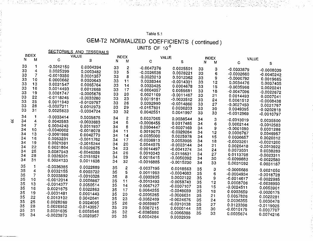
Table 5.1

GEM-T2 NORMALIZED COEFFICIENTS (continued)UNITS OF 10-6

SECTORIALS AND TE$SERALSINDEX VALUE INDEX VALUE INDEX VALUE

N M C S N M C S N M C S

33 1 -0.0012150 0.0004394 33 2 -0.0047376 0.0025501 33 3 -0.0033879 -0.000803933 4 0.0025399 0.0003482 33 5 -0,0026538 0.0028221 33 6 -0.0002660 -0.004024233 7 -0.0010350 0.0001357 33 8 -0.0023213 0:0012362 33 9 -0.0000792 0.001966533 10 0.0000662 0.0000643 33 11 0.0038344 -0.0014331 33 12 0.0034476 0.003740533 13 0,0031547 0.0065764 33 14 0.0033425 0.0004678 33 15 -0.0035966 0.002024133 16 0.0014493 0.0012668 33 17 -0.0004057 0.0055681 33 18 -0.0047096 -0.002267233 19 0.0061747 -0,0005676 33 20 0.0021109 -0.0011467 33 21 0.0014493 0.000704133 22 -0.0118245 -0.0033280 33 23 0.0019181 -0.0033512 33 24 0.0061512 -0.000843633 25 0.0011943 -0.0109797 33 26 0.0092990 -0.0014860 33 27 -0.0027450 0.002179733 28 -0.0027311 0.0012973 33 29 -0.0157601 0.0030203 33 30 0.0049395 -0.020281833 31 0.0025623 -0.0004724 33 32 0.0042551 0.0041997 33 33 -0.0012969 -0.0010797

34 1 -0.0033414 0.0005675 34 2 0.0037065 0.0038544 34 3 -0.0013019 0.003550034 4 0.0042593 -0.0033683 34 5 -0.0006455 0.0017485 34 6 0.0002144 -0.001258334 7 0.0034243 0.0011937 34 8 0.0004447 -0.0007169 34 9 -0.0001090 0.000128634 10 -0.0040002 -0.0018078 34 11 0.0019073 -0.0029264 34 12 0.0006767 0.004695734 13 -0.0061986 0.0042770 34 14 -0.0035000 0.0025978 34 15 0.0036657 0.002031234 16 0.0053231 -0.0011762 34 17 -0,0036913 0.0053905 34 18 -0.0023261 -0.002120034 19 0.0021381 -0.0015244 34 20 0.0044075 -0.0023144 34 21 0.0026418 -0.001392234 22 0.0031804 0.0029675 34 23 -0,0014497 -0.0041274 34 24 0.0073031 0.003828034 25 0.0087043 -0.0046268 34 26 0.0010343 70.0116631 34 27 0.0113708 -0.002331134 28 0.0026301 -0.0151921 34 29 0.0015415 -0.0050392 34 30 -0.0099883 -0.002258034 31 0.0024133 0.0011638 34 32 -0.0016885 -0.0015230 34 33 0.0031092 0.0031187

35 1 -0.0036385 0.0022889 35 2 -0.0037195 0.0018563 35 3 -0.0000686 0.002105035 4 0.0032155 0.0003722 35 5 0,0011993 -0.0004083 35 6 -0.0004934 -0.001872835 7 0.0003892 -0.0010328 35 8 -0.0003935 0.0002122 35 9 -0.0014617 -0.002298535 10 -0.0012014 0.0006867 35 11 -0.0013493 -0.0058743 35 12 0.0008706 -0.003695035 13 -0.0014377 0.0050514 35 14 -0.0067127 -0.0007107 35 15 -0.0024511 0.005390135 16 0.0021675 0.0022863 35 17 0.0064255 -0.0048059 35 18 0.0003659 -0.002017535 19 -0.0031481 0.0001443 35 20 -0.0005265 -0.0006631 35 21 0.0057826 0.002228135 22 0.0013102 0.0042641 35 23 -0.0052469 -0.0024676 35 24 0.0036355 0.003047635 25 0.0028269 0.0024095 35 26 -0.0059897 -0.0010138 35 27 0.0123398 -0.011902535 28 0.0026952 -0.0143957 35 29 0.0087215 0.0000144 35 30 -0.0010179 0.000770735 31 0.0031635 0.0058546 35 32 -0.0085880 -0.0066388 35 33 0.0035674 0.007421635 34 -0.0023873 -0.0020957 35 35 0.0004264 0.0002939

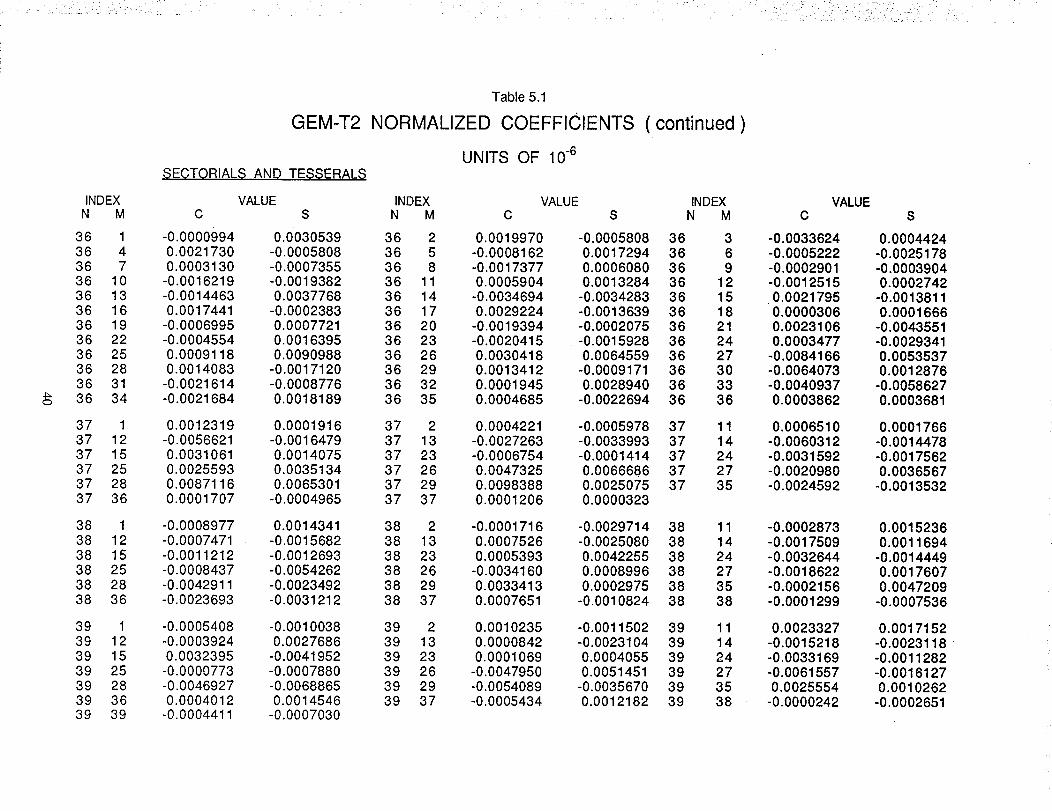
Table 5.1

GEM-T2 NORMALIZED COEFFICIENTS (continued)

UNITS OF 10-6$EOTORIALS AND TE$$ERAL$

INDEX VALUE INDEX VALUE INDEX VALUEN M C S N M C S N M C 8

36 1 -0.0000994 0.0030539 36 2 0.0019970 -0.0005808 36 3 -0.0033624 0.000442436 4 0.0021730 -0.0005808 36 5 -0.0008162 0.0017294 36 6 -0.0005222 -0.002517836 7 0.0003130 -0.0007355 36 8 -0.0017377 0.0006080 36 9 -0.0002901 -0.000390436 10 -0.0016219 -0.0019382 36 11 0.0005904 0.0013284 36 12 -0.0012515 0.000274236 13 -0.0014463 0.0037768 36 14 -0.0034694 -0.0034283 36 15 0.0021795 -0.001381136 16 0.0017441 -0.0002383 36 17 0.0029224 -0.0013639 36 18 0.0000306 0.000166636 19 -0.0006995 0.0007721 36 20 -0.0019394 -0.0002075 36 21 0.0023106 -0.004355136 22 -0.0004554 0.0016395 36 23 -0.0020415 -0.0015928 36 24 0.0003477 -0.002934136 25 0.0009118 0.0090988 36 26 0.0030418 0.0064559 36 27 -0.0084166 0.005353736 28 0.0014083 -0.0017120 36 29 0.0013412 -0.0009171 36 30 -0.0064073 0.001287636 31 -0.0021614 -0.0008776 36 32 0.0001945 0.0028940 36 33 -0.0040937 -0.005862736 34 -0.0021684 0.0018189 36 35 0.0004685 -0.0022694 36 36 0.0003862 0.0003681

37 1 0.0012319 0.0001916 37 2 0.0004221 -0.0005978 37 11 0.0006510 0.000176637 12 -0.0056621 -0.0016479 37 13 -0.0027263 -0.0033993 37 14 -0.0060312 -0.001447837 15 0.0031061 0.0014075 37 23 -0.0006754 -0.0001414 37 24 -0.0031592 -0.001756237 25 0.0025593 0.0035134 37 26 0.0047325 0.0066686 37 27 -0.0020980 0.003656737 28 0.0087116 0.0065301 37 29 0.0098388 0.0025075 37 35 -0.0024592 -0.001353237 36 0.0001707 -0.0004965 37 37 0.0001206 0.0000323

38 1 -0.0008977 0.0014341 38 2 -0.0001716 -0.0029714 38 11 -0.0002873 0.001523638 12 -0.0007471 -0.0015682 38 13 0.0007526 -0.0025080 38 14 -0.0017509 0.001169438 15 -0.0011212 -0.0012693 38 23 0.0005393 0.0042255 38 24 -0.0032644 -0.001444938 25 -0.0008437 -0.0054262 38 26 -0.0034160 0.0008996 38 27 -0.0018622 0.001760738 28 -0.0042911 -0.0023492 38 29 0.0033413 0.0002975 38 35 -0.0002156 0.004720938 36 -0.0023693 -0.0031212 38 37 0.0007651 -0.0010824 38 38 -0.0001299 -0.0007536

39 1 -0.0005408 -0.0010038 39 2 0.0010235 -0.0011502 39 11 0.0023327 0.001715239 12 -0.0003924 0.0027686 39 13 0.0000842 -0.0023104 39 14 -0.0015218 -0.002311839 15 0.0032395 -0.0041952 39 23 0.0001069 0.0004055 39 24 -0.0033169 -0.001128239 25 -0.0000773 -0.0007880 39 26 -0.0047950 0.0051451 39 27 -0.0061557 -0.001612739 28 -0.0046927 -0.0068865 39 29 -0.0054089 -0.0035670 39 35 0.0025554 0.001026239 36 0.0004012 0.0014546 39 37 -0.0005434 0.0012182 39 38 -0.0000242 -0.000265139 39 -0.0004411 -0.0007030

Table 5.1

GEM-T2 NORMALIZED COEFFICIENTS (continued)

UNITSOF 10"sSECTORIALS AND TESSERALS

INDEX VALUE INDEX VALUE INDEX VALUEN M C S N M C S N M C S

40 1 0.0003977 0.0011647 40 2 -0.0003638 -0.0015783 40 11 0.0006976 -0.000629440 12 0.0002103 0.0002648 40 13 -0.0023484 -0.0033431 40 14 0.0000423 0.001045240 15 0.0001404 0.0025006 40 23 0.0011245 -0.0014907 40 24 0.0004783 0.001883640 25 -0.0007236 -0.0024068 40 26 0.0050145 0.0015346 40 27 -0.0009711 -0.000262340 28 0.0017698 0.0040420 40 29 0.0010936 0.0002024 40 35 0.0009078 -0.002776040 36 0.0013914 0.0029042 40 37 -0.0016385 0.0016023 40 38 -0.0002456 0.000901440 39 0.0004278 -0.0008566 40 40 -0.0007832 0.0004286

41 1 -0.0012735 -0.0002474 41 2 -0.0003915 -0.0001628 41 11 0.0001253 0.000812541 12 0.0027148 0.0011758 41 13 0.0016950 0.0037141 41 14 0.0011678 0.003315041 15 0.0001752 -0.0021864 41 23 0.0001894 0.0006816 41 24 0.0017087 -0.000041341 25 -0.0018848 0.0011051 41 26 0.0047837 -0.0080686 41 27 -0.0011405 0.001450941 28 -0.0042768 -0.0009932 41 29 0.0002297 0.0023047 41 35 0.0005460 0.000461441 36 -0.0011322 -0.0010519 41 37 0.0005529 -0.0017954 41 38 -0.0000004 0,001034141 39 -0.0003088 -0.0005950 41 40 0.0004386 -0.0004779 41 41 0.0003718 0.0000932

42 1 0.0005314 -0.0005602 42 2 0.0006463 -0.0005361 42 11 0.0012176 -0.000367242 12 0.0014837 -0.0010948 42 13 -0.0001945 -0.0001583 42 14 -0.0004083 -0.001631042 15 -0.0014494 0.0009136 42 23 0.0003650 -0.0014766 42 24 0.0011082 -0.000296042 25 0.0007718 0.0029789 42 26 -0.0043012 -0.0032607 42 27 0.0026574 -0.001315242 28 -0.0001477 0.0038958 42 29 -0.0038343 0.0007940 42 35 -0.0011902 0.000285142 36 0.0020302 0.0001011 42 37 0.0000419 -0.0010701 42 38 0.0008246 -0.001310742 39 -0.0004072 0.0018459 42 40 0.0014332 -0.0007298 42 41 -0.0007583 0.001177342 42 -0.0003950 0.0006384

43 1 -0,0000801 0,0006980 43 2 -0.0009052 0.0002684 43 11 -0.0012732 -0.000321943 12 0,0006744 -0.0008274 43 13 0.0021243 0.0006238 43 14 -0.0015029 0.002786443 15 -0.0011884 0.0003396 43 23 0.0004332 -0.0001977 43 24 0.0009323 0.001051343 25 -0.0000106 -0.0000279 43 26 -0,0038657 0,0002359 43 27 0.0064481 0.004094143 28 -0.0009041 0.0088787 43 29 -0.0030416 -0.0001038 43 35 -0.0014784 -0.000816543 36 0.0009173 -0.0010471 43 37 0.0004137 0.0004758 43 38 0.0005844 -0.000762843 39 0.0000636 0.0009355 43 40 0.0006770 -0.0018402 43 41 0.0003727 0.000684343 42 -0.0000040 0.0014679 43 43 0.0005206 -0.0003446

900_LO0"O 89Z_000"0- 8_ Z# 9LO_O00"O- 9L9LO00"O _# L_LO_6_O0"O LOL_O0"O- L_ L_ _£98000"0 #_000"0- O_ Z# _Z6ZO00"O L99LO00"O 6_ L_999L000"0 LL89000"O 98 Z_ 6809000"0 0L6£000"0 L8 Z_ 99Z#000"0- _96_000"0 98 L_9_9_000"0- 9_£Z000"0 £8 Z_ 9_ZLO00"O- _L9_O0"O 6_ Z_ #_L900"O- L_LO0"O- 9_ Z_ZZO_O00"O- #_LLO00"O L_ Z# ZSL9000"O- 6L6£_00"0 9_ Z# 6#L£000"0- 0_£0000"0 £_ Z__SZ_O00"O- 99L_000"0- _ Z_ L_6_O00"O _998000"0- 8_ L_ _968000"0- L66#000"0- £L Z#_S_O0"O- L668000"0 #_ Z_ 0_6_000"0- 99L£000"0- 8L Z# 69Z0000"0- OL90000"O _ L_89_0000"0- 9LSLO00"O _ L_ SS90000"0- _0_8000"0 _ Z# _9L_O00"O- 9L9_000"0 L L_

£L_L900"O L966_00"0- 8_ 9_ LL_8000"O 99L9_00'0 _# 9_L66L_O0"O 9060L00"0 L_ 9_ 90L_O0"O- 9_#9L00"0 O_ 9_ _09LO00"O- _8_000"0 68 9_99_L000"0 9L9_000"0 98 9_ L999000"0- L_6000"O- L8 9_ 986_000"0- 8_LLO00"O- 98 9_69L6000"0 L9LO000"O 98 9_ 8LO_O00"O- _S6_LO0"O 6_ 9_ 9_LL900"O- _000"0- 9_ 9#L080_O0"O 6L9L_O0"O- L_ 9_ 9L06_00"0 06_6000"0 9_ 9_ _9_00"0- _80LO00"O 9_ 9_9_L_O00"O LLO_O00"O- _ 9_ 9998000"0 996L000"0- 8_ 9_ 9_LO00"O- #LSgO00"O- £L 9_9909000"0 909_000"0- _L 9_ LgL_O00"O- LgL_O00"O- EL 9_ 699L000"0- L99LO00"O- _L 9__9_8000"0 96L9000"0- LL 9_ 0968000"0 9_#000"0- _ 9_ 9_88000"0- £LO_O00"O _ 9_

999L000"0 _8_00"0- 8_ 9_ 9_L_O0"O- 9908000"0 _ 9_L_O_O0"O- 969_000"0- _ 9_ L6L_O00"O 69L0000"0 O# 9_ 99L_LO0"O- 96_000"0- 68 9_0998000"0- LZO_LO0"O- 88 9_ 9_6_000"0 9_96000"0- L8 9_ _LOgLO0"O 0_000"0- 98 £_9_99000"0 9L#9000"0- 98 9_ O0£_LO0"O- 9L99LO0"O- 6_ 9_ 9_99L00"0 988_00"0 9_ 9#_8L_800"0- Z£L9800"O- Z_ 9_ 866_L00"0 _L9LO00"O- 9_ 9_ 66#0000"0- 9L88000"0 9_ 9_L968000"0 L99_000"0- _ 9_ 99L8000"0- 9_9L000"0 8_ 9# 900_LO0"O _Z_O000"O £L 9__80L_O0"O- L6_O00"O _ 9_ 9999L00"0- 69LLO00"O- 8_ 9_ _99000"0- L998000"0- _ 9_0690000"0 _L_LO00"O LL 9_ 60_0000"0- 898_000"0 _ 9_ LS_O00"O 9869000"0 L 9#

9LL_800"O- 9_8800"0 8# #_ _#6LLO0"O- L9LLO00"O- _ _L8_8800"0- _8_9000"0 L_ #_ _96_00"0 89Z9_00"0- O# _ 990_000"0- _L£O00"O 68 _00_0000"0 L89LO00"O- 98 _ 8_9000"0 L_O_O0"O L8 #_ 8899000"0- 9L9_00"0- 98 _0_09000"0- _9_000"0 98 #_ _0_00"0 LO_O_O0"O- 6_ _ 8_L9000"0 OL09000"O- 8_ _6_ZOLO0"O" _LS_O0"O L_ #_ 88L_000"0 _69000"0 9_ _# 96_8000"0 0896000"0- 9_ _09_9000"0- Z860000"0- _ #_ 9_L8_00"0 9Lt9000"O- 8_ _ 800_000"0- 900_000"0 £L _999_L00"0- Lgzo000"O _L #_ 068_00"0 99L_00"0 EL #_ 6099000"0- OZS_O00"O _L _680_000"0 9LO_O00"O- LL _ 9_0_000"0 L_98000"0 _ #_ 6L98LO0"O- Z098000"0 _ _

S 0 _ N S O _ N S 0 _ N3_7VA X30NI 3nqvA X30NI 3_7VA XBONI

37V_39931 ONV 97VI801039

9.0L _0 S±IN_

(penu!;uoo) 3±N910199900 Q3ZIqVIAINON ±-1 139V9 alqe±

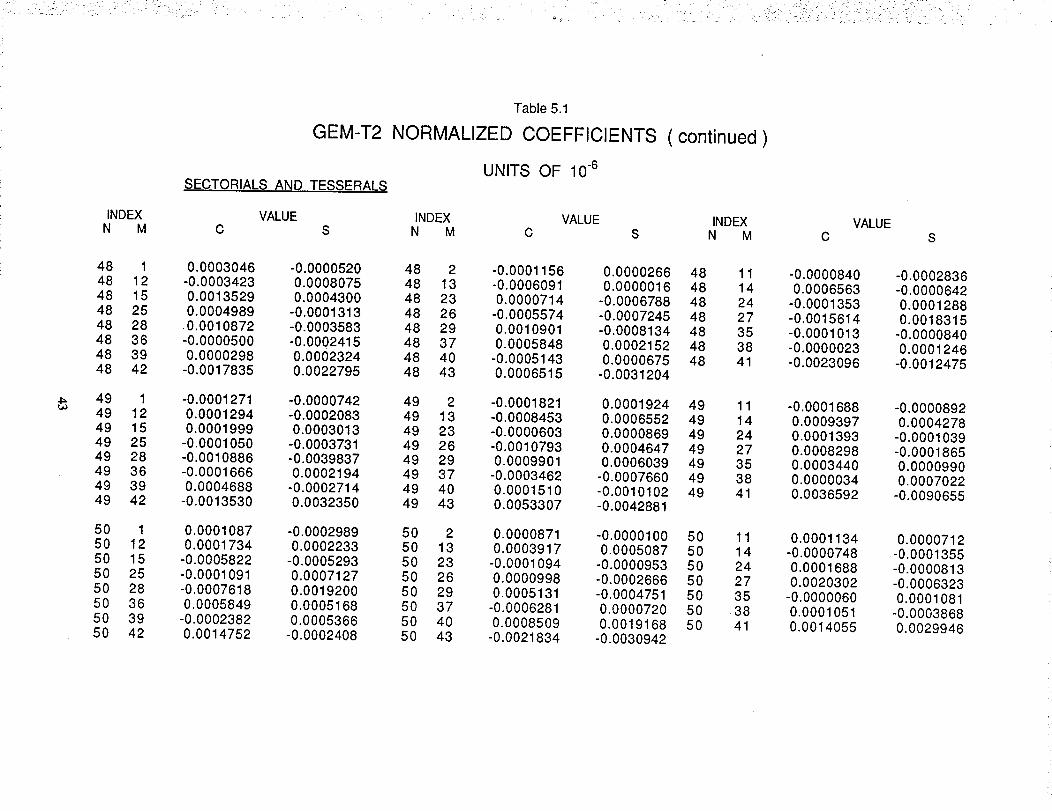
Table 5.1

GEM-T2 NORMALIZED COEFFICIENTS (continued)

UNITS OF 106SECTORIALS AND TESSERALS

INDEX VALUE INDEX VALUE INDEX VALUEN M C S N M C S N M C S

48 1 0.0003046 -0.0000520 48 2 -0.0001156 0.0000266 48 11 -0.0000840 -0.000283648 12 -0.0003423 0.0008075 48 13 -0.0006091 0.0000016 48 14 0.0006563 -0.000064248 15 0.0013529 0.0004300 48 23 0.0000714 -0.0006788 48 24 -0.0001353 0.000128848 25 0.0004989 -0.0001313 48 26 -0.0005574 -0.0007245 48 27 -0.0015614 0.001831548 28 •0.0010872 -0.0003583 48 29 0.0010901 -0.0008134 48 35 -0.0001013 -0.000084048 36 -0.0000500 -0.0002415 48 37 0.0005848 0.0002152 48 38 -0.0000023 0.000124648 39 0.0000298 0.0002324 48 40 -0.0005143 0.0000675 48 41 -0.0023096 -0.001247548 42 -0.0017835 0.0022795 48 43 0.0006515 -0.0031204

49 1 -0.0001271 -0.0000742 49 2 -0.0001821 0.0001924 49 11 -0.0001688 -0.000089249 12 0.0001294 -0.0002083 49 13 -0.0008453 0.0006552 49 14 0.0009397 0.000427849 15 0.0001999 0.0003013 49 23 -0.0000603 0.0000869 49 24 0.0001393 -0.000103949 25 -0.0001050 -0.0003731 49 26 -0.0010793 0.0004647 49 27 0.0008298 -0.000186549 28 -0.0010886 -0.0039837 49 29 0.0009901 0.0006039 49 35 0.0003440 0.000099049 36 -0.0001666 0.0002194 49 37 -0.0003462 -0.0007660 49 38 0.0000034 0.000702249 39 0.0004688 -0.0002714 49 40 0.0001510 -0.0010102 49 41 0.0036592 -0.009065549 42 -0.0013530 0.0032350 49 43 0.0053307 -0.0042881

50 1 0.0001087 -0.0002989 50 2 0.0000871 -0.0000100 50 11 0.0001134 0.000071250 12 0.0001734 0.0002233 50 13 0.0003917 0.0005087 50 14 -0.0000748 -0.000135550 15 -0.0005822 -0.0005293 50 23 -0.0001094 -0.0000953 50 24 0.0001688 -0.000081350 25 -0.0001091 0.0007127 50 26 0.0000998 -0.0002666 50 27 0.0020302 -0.000632350 28 -0.0007618 0.0019200 50 29 0.0005131 -0.0004751 50 35 -0.0000060 0.000108150 36 0.0005849 0.0005168 50 37 -0.0006281 0.0000720 50 38 0.0001051 -0.000386850 39 -0.0002382 0.0005366 50 40 0.0008509 0.0019168 50 41 0.0014055 0.002994650 42 0.0014752 -0.0002408 50 43 -0.0021834 -0.0030942

• L

' :: wavenumbers of interest for orbital computations than are the ocean tidal terms at the same_ wavenumbers.

However, one must exercise caution when comparing dynamic satellite solutions for ocean_: tidal terms with those obtained oceanographieally. Firstly, oceanographic measurements are

_ relative to a land or sea-bottom reference while the effects sensed by satellite data aregeocentrically referenced. More importantly, the satellite experiences a changing gravitationalattraction which results from all mass redistribution within the Earth/ocean/atmospheric system.Within the semi-diurnal and diurnal bands, clearly tidal effects are dominant and a comparisonbetween ocean models and satellite solutions is reasonably straightforward under the assumption

.... that the solid Earth tides have been well modeled. However, at monthly, semi-annual, annual andlonger periods, there are important climatological effects (e.g. Gutierrez and Wilson, 1988),changes in the hydrosphere pertaining to ground water retention cycles and the volume of waterstored in continental aquifers (e.g. Chao, 1988), in snow cover (e.g. Chao and O'Connor, 1988) andother sources of mass redistribution which are not "tidal" in origin, and certainly not isolated tochanges in the ocean surface at these periodicities. We believe that the large value we obtainedfor the Sa tide at third degree represents north to south hemispheric mass transport effects withan annual cycle which is not of a tidal origin. This coefficient is large, but at the same time, itseems well determined within our analysis. However, radial non-conservative force modeling errors

• ! may be accomodated by an adjustment of this term.

Although admitting to these limitations, we have in the past compared our tidal solutionswith both ocean models and other satellite solutions. These comparisons are found inChristodoulidis et al., (1988). While these comparisons will not be repeated herein, it is fair tosay that GEM-T2 compares equally well with the results given for GEM-T1 within this reference.

Table 5.2 presents the GEM-T2 tidal solution. It has been compared with the solution• developed in GEM-T1 (given in Marsh et al., 1988) and overall, the agreement is very good.

Principally, in GEM-T2 we were able to extend the solution for the m=0 long period tidal bandto include a third degree coefficient for the Sa, Ssa, Mfand Mm lines. In the diurnal band (m= I),the solution for O1, P1, and K1 has been extended to include the adjustment of terms of degree5. Further, within the semi-diurnal band, where m=2, a solution containing terms of degree 6has been performed for K2, $2, M2, N2, and T2 tide lines. In each case, an additional degreeabove GEM-TI's cutoff was accomplished with 90 adjusting coefficients in the GEM-T2 solution.

44

....:i•Table 5.2

GEM-T2 Dynamic Ocean Tidal Model

i_ Darwinian Name/

Constituent Values Uncertainties

,_ Tide Degree Order Amplitude Phase Amplitude Phase

• iii: (cm) (deg) (cm) (de_g)

: -- Long Period Band * --

Mm 2 0 0.740 256.318 0.317 23.973Mm 3 0 0.814 16.653 0.673 46.210

Sa 2 0 3.033 28.771 0.404 8.034.... Sa 3 0 6.472 320.140 0.574 5.210

: • Mf 2 0 2.069 237.076 0.312 8.662Mf 3 0 1.032 354.630 0.827 42.651

Ssa 2 0 1.276 249.472 0.415 17.933i Ssa 3 0 0.866 89.398 0.560 36.494

-- Diurnal Band --

K1 2 1 2.845 325.513 0.165 3.349K1 3 1 0.903 14.513 0.109 7.145K I 4 1 2.487 258.163 0.208 4.895

: K1 5 1 2.184 106.526 0.215 5.676

O 1 2 1 2.717 315.443 0.128 2.688O1 3 1 1.390 83.019 0.151 6.271O 1 4 1 1.904 279.743 0.2 I0 6.197Ol 5 1 1.520 118.638 0.210 7.830

P I 2 1 I. 105 313.188 0.167 8.650P 1 3 1 0.344 359.467 0.109 18.970P 1 4 1 0.837 262.941 0.212 14.419P 1 5 1 0.442 148.854 0.216 27.769

-- Semi-Diurnal Band --

K2 2 2 0.319 313.503 0.043 7.775K2 3 2 0.231 189.952 0.040 7.468K2 4 2 0.169 112.652 0.043 14.517K2 5 2 0.079 96.276 0.034 23.516

_ K2 6 2 0.043 203.524 0.045 59.854

M2 2 2 3.320 321.257 0.047 0.814M2 3 2 0.304 156.469 0.056 10.574M2 4 2 0.994 127.174 0.046 2.669M2 5 2 0.290 8.059 0.036 6.943

_ M2 6 2 0.403 320.819 0.049 6.946

.... • symmetries exist in the harmonic expansion of the m=0 tides so that the values represent thesums of the C + and C- (prograde and retrograde) terms (see Christodoulidis et al., 1988: AppendixA).

45

r_ " •

; -- Semi-Diurnal Band (continued) --

$2 2 2 0.831 300.412 0.044 3.017

ii _ $2 3 2 0.328 221.479 0.034 6.079$2 4 2 0.333 87.229 0.042 7.639$2 5 2 0.136 9.561 0.032 15.998

_ $2 6 2 0.215 284.419 0.044 12.013

N2 2 2 0.678 334.416 0.061 5.171N2 3 2 0.088 155.802 0.060 39.477N2 4 2 0.250 139.018 0.049 1 I. 169

: N2 5 2 0.094 341.627 0.037 22.892• N2 6 2 0.059 3.215 0.054 52.701

T2 2 2 0.046 273.217 0.044 55.890T2 3 2 0.005 119.652 0.034 420.136T2 4 2 0.036 242.628 0.045 72.181

_' T2 5 2 0.088 70.699 0.033 21.134T2 6 2 0.042 22 I. 127 0.047 63.835

i _

!_:!i

'.: 5.3 Tidal Braking in the Earth/Moon/Sun System Using Dynamic Tide Model of GEM-T2:_ : >,

!:>:' Modern satellite tracking systems allow us to monitor the orbital motion of near-Earthsatellites to unprecedented levels of accuracy. The GEM-T2 geopotential is a model which usesthese observations to deduce both the static and tidal potential fields. The complete GEM-T2

' ii_ tidal model containing both the adjusted and unadjusted terms has been used to estimate the! effects of the Earth's tides on the Earth/Moon/Sun system. The solid Earth tidal model which is

> ,: used has no phase angle (Wahr, 1981) so it is free of dissipation, but any residual phase due to:::.: anelastic properties of the solid Earth would be compensated for in the adjusting ocean tidal

coefficient set of GEM-T2 for the twelve major tidal frequencies which are allowed to adjust.Therefore, this model should accurately reflect the external tidal potential sensed on Earth

',= orbiting satellites and can be used directly to infer the tidal contribution to the exchange ofangular momentum within the Earth/Moon and Earth/Sun systems.

. Using the development given in Christodoulidis et el., (1988), we have calculated the...... secular change in the mean motion of the Moon and the tidal braking in the Earth's rotation

rate using GEM-T2. Table 5.3 presents a comparison of the GEM-T1 and GEM-T2 tidal

constituents when used to compute these two effects. The secular change in the lunar mean: _ motion estimated from GEM-T2 is -26.6 ± .5 arcsec century -2 which can be compared with GEM-

TI's implied value of-25.3 - .6. The major difference in the models is the change in the seconddegree value for the Mf tide (both in amplitude and phase) and a small change in second degree

:__ M2 which increased slightly in amplitude. These changes combine to move the GEM-T2 value forthe calculated secular change in the lunar mean motion further away from the value beingobtained from lunar laser ranging which is -24.9 _ 1.0 (Newhall et al., 1986).

The tidal braking of the rate of the Earth's rotation due to conservation of angularmomentum in the Earth/Moon/Sun system yields a value of -6.31 ± .16 x 10 "22 rad S "2. GEM-T1 yielded a value of -5.98 ± .22. Taking into account the effect of the secular change in thesecond degree zonal harmonic as given by Yoder et al., (1983) of 1.29 +--0.28 when mapped into

< the braking of the Earth's rotation rate (see Christodoulldis et al., 1988 and Bursa, 1986),artificial satellites give a combined value of 5.02 ± 0.32 and 4.69 ± 0.36 x 10 -22 rads "2 for GEM-

i' T2 and GEM-T1 respectively. These values are consistent with recent astronomic studies (e.g.Stephenson and Morrison, 1984) who find a value of 2.4 ms/century for eclipse records prior to1620 and 1.4 ms/century for telescopic data since 1620. The GEM-T2 and GEM-T1 valuescorrespond to 1.88 and 1.76 ms/century.

5.4 The GEM-T2 Earth Rotation and Polar Motion Series

The GEM-T2 solution is based on tracking data spanning the period from mid-1960 to: : mid-1987. The quality of the data is not uniform at all; it has therefore been decided that

the reference frame be adjusted only during the years when the data contains robust subsets': : : of high quality laser tracking on such satellites as Lageos, Starlette and Ajisai. This translates

to the period from 1980 onward.

" The definition of the adopted reference sYstem and its realization has been discussed•..... extensively in Marsh et al., (1988). The most important features which we will need for the

' present are the fact that the apriori series is based on a combination of BIH and Lageos SL6-.::: derived values. The series have been compared over a 6-year overlapping period and the resulting< ii

transformation applied to the BIH segment to put it in the SL6 frame. Finally, the average of the.... pole coordinates over the 6 years 1979-84 has been subtracted to create the apriori series in

_.: a coordinate system with an origin that is nearly coincident with the center of the wobble. This: : results in a systematic offset of the TOPEX/Poseidon solution reference frame to that of IERS(BIH)

: or SL7.1 of some 38 mas in the x component, and 280 mas in the y component.

i_ 47

.... ¢

Table 5.3 Comparison of GEMoT1 and GEM-T2 Dynamic Tide Models

:_-i, for Secular Change in the Mean Motion of the Moon (n)

: '_ and in the Rotational Velocity of the Earth (_)" 4

Tide • GEM-T 1 • GEM-T2

n o n n o n

• units: arcsec century "2

: 056.554 Sa 0.00 0.00 0.00 0.00

_, :,, 057.555 Ssa -0.00 0.00 -0.00 0.00058.554 0.00 0.00 0.00 0.00065.455 Mm -0.03 0.31 -0.13 0.12075.555 Mf -0.56 0.18 -1.18 0.16075.565 -0.10 0.06 -0.10 0.06

135.655 Q1 -0.18 0.04 -0.18 0.04145.545 Olf -0.10 0.02 -0.10 0.02145.555 Ol -2.92 0.25 -3.12 0.21155.455 Mlf 0.00 0.00 0.00 0.00155.655 M1 0.01 0.00 0.01 0.00162.556 rr i -0.00 0.00 -0.00 0.00163.555 P 1 -0.00 0.00 -0.00 0.00164.556 S 1 0.00 0.00 0.00 0.00165.545 Klf ................165.555 K1 moon ................165.555 K1 sun ................165.565 Kls ................166.554 xtr 1 0.00 0.00 0.00 0.00167.555 _b1 0.00 0.00 0.00 0.00175.455 J1 0.01 0.00 0.01 0.00185.555 OO 1 -0.00 0.00 -0.00 0.00

245.655 N2 -1.43 0.16 -1.39 0.14255.545 M2s 0.02 0.01 0.02 0.01255.555 M2 -20.00 0.40 -20.44 0.39265.455 L2 0.01 0.00 0.01 0.00

: 271.557 0.00 0.00 0.00 0.00272.556 T2 -0.00 0.00 -0.00 0.00273.555 $2 -0.00 0.00 -0.00 0.00274.554 R2 0.00 0.00 0.00 0.00275.555 K2 moon ................275.555 K2 sun ................285.455 0.00 0.00 0.00 0.00

_i 295.555 0.00 0.00 0.00 0.00

total -25.27 0.61 -26.61 0.51

_!

i_:i I

?,

_i!ii

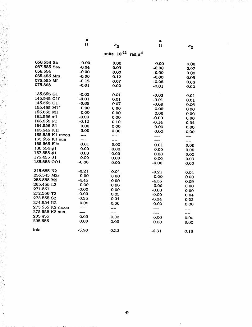
_,_ _ o_ _ o_

::: units: 10 "9+2 rad s "2

056.554 Sa 0.00 0.00 0.00 0.00:+ 057.555 Ssa -0.04 0.03 -0.08 0.07

058.554 -0.00 0.00 -0.00 0.00+i.+,i 065.455 Mm -0.00 O. 12 -0.00 0.05+ • _ 075.555 Mf -0.12 0.07 -0.26 0.06:: :" 075.565 -0.01 0.02 -0.01 0.02

135.655 Q 1 -0.03 0.01 -0.03 0.01

145.545 Olf -0.01 0.01 -0.01 0.01145.555 O1 -0.65 0.07 -0.69 0.06155.455 Mlf 0.00 0.00 0.00 0.00

: 155.655 M1 0.00 0.00 0.00 0.00162.556 Ir I -0.00 0.00 -0.00 0.00

,i: 163.555 P1 -0.12 0. I0 -0.14 0.04164.556 $1 0.00 0.00 0.00 0.00165.545 Klf 0.00 0.00 0.00 0.00165.555 K1 moon ................

_ 165.555 K1 sun ..... ..... ____ ____

165.565 Kls 0.01 0.00 0.01 0.00166.554 _1 0.00 0.00 0.00 0.00167.555 ¢ I 0.00 0.00 0.00 0.00175.455 J1 0.00 0.00 0.00 0.00185.555 OO 1 -0.00 0.00 -0.00 0.00

: 245.655 N2 -0.21 0.04 -0.21 0.04255.545 M2s 0.00 0.00 0.00 0.00255.555 M2 -4.45 0.09 -4.55 0.09

.... _ 265.455 L2 0.00 0.00 0.00 0.00• 271.557 -0.00 0.00 -0.00 0.00

272.556 T2 -0.00 0.05 -0.00 0.04• 273.555 S2 -0.35 0.04 -0.34 0.03

274.554 R2 0.00 0.00 0.00 0.00275.555 K2 moon ........275.555 K2 sun ........

: 285.455 0.00 0.00 0.00 0.00295.555 0.00 0.00 0.00 0.00

total -5.98 0.22 -6.31 O. 16

49

r

The estimated Earth Orientation Parameter (EOP) series are displayed in Figures 5.1through 5.4, their formal (unsealed) accuracies are shown in Figures 5.5, 5.6, and 5.7. Thedifferences of the estimated coordinates of the pole from the apriori values are plotted in Figures

_ 5.8, 5.9 and 5. I0. The results are remarkably close, within 0.5 mas, to those obtained withthe GEM-T1 solution. The systematic bias of some 17 mas in the y component is now well

i__! understood and its source is an erroneous transformation of part of the apriori series. Because- ..... the adjustment in the pole is free, the error only affects the display. The RMS about the meani!_/, for these corrections to the apriorl are 4.2 mas for the x component and 3.5 mas for the y_ii, I component. These values are nearly identical to those within the GEM-TI solution.

_ To further evaluate the solved EOPs we compared the common part of our solution tothat of the VLBI-based IRIS series. The overlapping period is 84/01/05 to 87/02/18.

_.... Transformation parameters estimated from this comparison are given in Table 5.4. Our origin,- is very consistent with that of IRIS once we have accounted for all the systematic differences

between frames. Of more interest, however is the agreement between the series when thesystematics are eliminated. The RMS differences in x and y are 2.2 mas and 2.5 masrespectively, and 0.4 msec and 0.16 msee for Earth rotation (A. 1-UTIR) and length of day (LODR)correspondingly. If we assume that the errors between the two series are random anduncorrelated, which is realistic since they come from independent techniques and data sets,then the above RMSs can be multiplied by 0.707 to give the individual series uncertainties.This results in realistic error estimates for polar motion at about 1.5 mas and length of dayvariations at 0.1 msec.

5.5 GEOSAT TRANET Station Coordinates

In general, the station positions were held fLxed in our GEM-T2 solution as was done for

GEM-T1. These aprlori station coordinates were predominantly based on the ultra-precisegeodetic positioning available from LAGEOS laser ranging analyses. Available geodetic surveyties were extensively used enabling older systems to be tied into the laser-described geocentricnetwork. Other methods were required to secure good coordinates for all of the differenthistorical tracking systems; this included using network analyses which were used to relateprevious Unified S-Band and TRANET Doppler station solutions into the TOPEX/Poseidonreference system.

For our GEOSAT analyses however, we only had DMA TRANET II positions available forGEM-T2. These stations required positioning within the TOPEX/Poseidon reference frame, buti

lacked suitable common stations with earlier solutions to effect these ties. This was not aproblem encountered with our TRANET analyses performed using SEASAT data because lasertracking was also available on SEASAT and the Doppler positions were derived from the satellite

positioning solutions directly. Even though approximately ten of the same geographic locationscommonly were occupied between the GEOSAT timeframe and that of SEASAT, the local station

eccentricity data linking the electronic centers of the instruments to their corresponding surveymarkers was not available. Instrument maintenance and system upgrades had occurred at allsites since the SEASAT era which precluded simple transformations to obtain appropriateGEOSAT tracking station coordinates. Consequently, we elected to adjust the GEOSAT TRANETII stations within GEM-T2.

Our 80-day set of GEOSAT tracking data starting at the beginning of the ERM repeatmission was utilized for this coordinate determination. This data set had representation fromthe complete TRANET Network of nearly 50 stations. These solved-for coordinatesare availablefrom the authors upon request.

Table 5.5 compares our adjusted GEOSAT station coordinates with the WGS-84 positionsavailable from DMA. The RMS of fit in the intercomparison is better than 0.5 m in each

coordinate after removal of a seven-parameter Wolf-Bursa transformation. Considering theDoppler coordinates are not likely to be derivable from this type of tracking data to better than

• about 30 cm in each coordinate, this level of agreement is considered quite good. The

50

Ear'-T_h Or'- [ enact [ on Pi_r'-arnel;,eps f'Pom GEM-T2

TOPEX GRFIVZTY FIELD 60LUTION t PG6-54qB

40_ .....................................................................................................................................................................................................................................................................................................................ii

i

J

7 _ ++': i i +:_ _+, i%. i i

2,_<_.............................................................i..............................................................E..................................._......*..............i'"'"+"""_.......................-_'"_-........:.............................................................iilt_ + + _ + " zz_ i ,=,,,_ . .+ _ + _ :

i _ *" + + i i: ' + + i+ 41:-t- • ,z_ i :. _-_ + + t+ + +_71 +._ j1oz .............................................................j......................._ ........................... .+...................+............+.............,."...._..........+..................,+,.........._....';..............._......t................................,oE i t'"t _ + + + i + + + "_. _ :i i

i # % _ _ + + i+ + + -I- + _ iI_ U i .it i _i + 4- + : + 4- _'3" t, "

.... + + ++'+7..............'> _t..........................................................._.........#......................._.i............¢............._.................+............i..+_..............+..............+................_..................................iz 1 -i. i- _ -'ll .,. + + i + + T- @ _ i

I IV V _++ +i+++ + + !I g ++ '+ - �"+_- ; ._ + + •n-

Jo t_- +I ++

iii + !i i

i- 5 I;_.l;_liTl=l 1 Cl8_1 1Cl_ I clB4 1CtB6 I I=l_l_

CF:IL,E NDI=IR YERI_

Figure 5.2

Ear-t.h Or lentmtlon P_r_meters from GEM-T2

TOPEX r-R_VITY FIELD SOLUTION t PGS-54q8

40_ I.........................................................................................................................................................................................i.........................................................................................................................................................................................,............................................................._...........................................................".........................................................e.............................................................1

! : :

Z _ i_ -_- -I- .: 4- 4- + -I- ii ,,_""J_ + + • + + Ehi _ + - i+ + + + .,.z

o i _, _ g + _. i .+ + + +. I J_ in I _t_ ............................................................._......................._f_ ............................,4-........,_..................................t............._.....t..........._ ..................4,,..........t....._,..............._......_r_................................: -- _ : T "I" i" i .#'-'_ _ t + + i+ + .+ +i I _o i _ _,. _ _- + + i+ + -i- "t. j

_ f _r_ _ + + + " + + ._" _i _i + i + + "

...........................................................•_..........._ ......................_ .............-_..i.............+.............._ ................+............i.................+ .............._..............._._..........._................._...........................z _ _ _, _ + + + i+ + _ _i ¢ '_ io _ti + t i++ ; + t !o i_Im _F i + + _- i+ + + -t. _-

+ + ! + + :+_ t +

° i

+i

i5 w1._::117B_ 198 _1 11::18::_ 1 limB4 1 qB6 1 ¢:11_

I

CRL, ENDI=IR YEI=IR

Figure 5.2

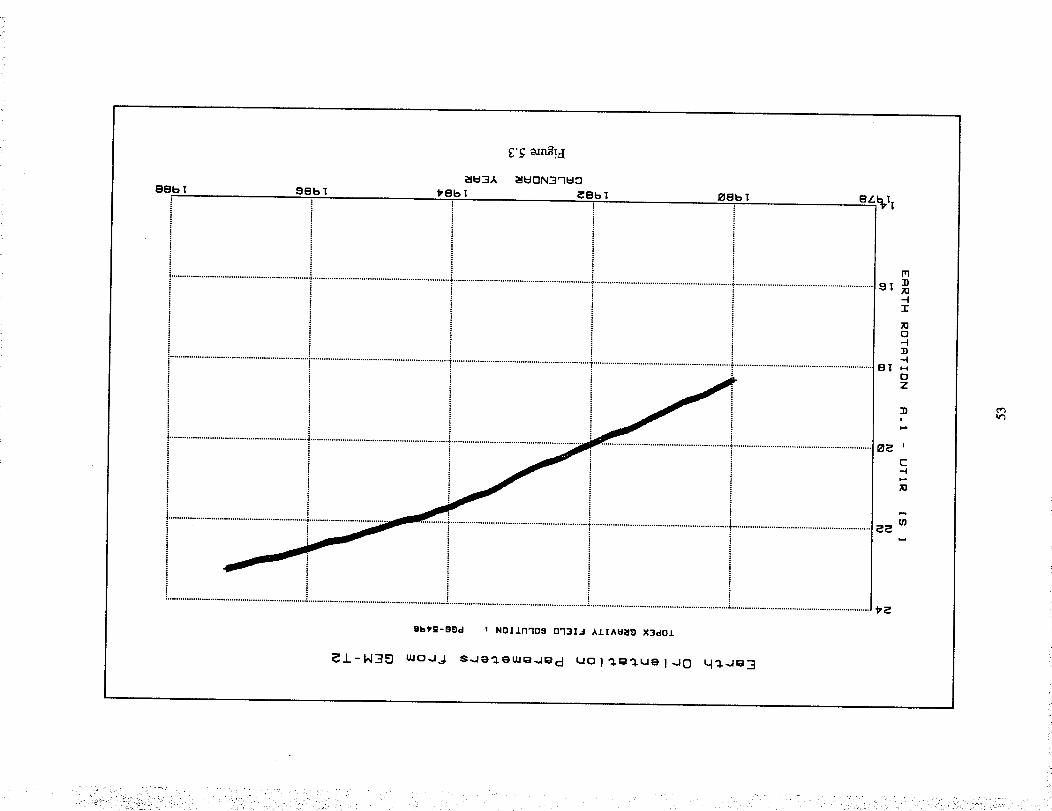
g'g mn_!_

88bT 986_ _86I _86I _861 8L_Iiv

i..............................................................................................................................................................................................._..................................................................................................................................8I _

I

Q

...................................................................................................................................................................................................._.................................................................................................................................81 _0Z

_ m

C

NN _

i !..................................................................:................................................................................................................................._................................................................................................................................._

EP, r-_h Or-lent, at, Ion Par-,,met, er-s f'r-om GEM-T2

TOPEX GRAVITY FIELD 80LUT[ON S PGE-54q@

500 ....................................................,....................................................._...............................................................................

, " i ii " " • " "' . " .' ..

E

• • _ i _.-- 200 ...........................:......-.................i....................:........ _.................._.........................."'....................................................

I-z . _. ."i" i "i ". ".hiZ . .i • .= _ _ • ".0 • . . : . :..,... ,. : -

0. 100 .........................;:................•........."................""":_:t:" .................."'_............................i: ...............:4...............................E

._ 0 • " " " . :" "'" :,. i ". •i" " " .._" " • .., i • . .':

X _, . ... _ ... . .4

Z • :. • "a •." . . .,0 • ". • :" _ • • i

• , .' ,:. • .

p , : . . : _ . • . :

0• . : • . . ... :

rv - 100 ........................:_.""'":...................!',........................i..................:......,".........:.....................................",...:.............................E ".:.- • i ".. .. i ." • • i .J

o i, • • _ i . i . "n

- 200 ..........................".............:..."........._........................._...................................................:i.....................................................• .i " • i . .." • • "

!' " "i'. • • i .

"5B-_300 -_00 -100 0 100 200 500 4B0

POLAR MOTION Y COMPONENT [MAS]

Figure 5.4

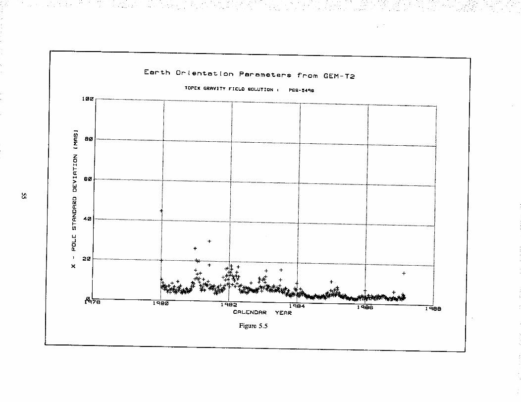
Emr_t.h Or _ t er_t.,mt:, [ or_ Pmr'-mmeC, er'-_ from GEH-T2

TOPEX GRRVITY I:'IEL, n @OI.,UTION t PG6-@4R@

100 ...............................................................................................................................................................................................................................................................................................................................

_" BO ..............................................................................................................................................................................................•.............................................................................................................................

" iZ

I---II

_ 60 .............................................................................................................................................................................................

t_ QNff 40Zff 40 ...............................................................................................................................................................................................-'...............................................................................................................................

gl

LdJ + i

a i' 20 ..............................................................Jr ............................._ ..........................................................................................._............................................................................................................................

x i + + _; + + + i +{ ++ + i

1"¢_178 19@0 1982 I qB4 1 '=186 I ct88

CAL, ENOAF_ YEAR

Figure 5.5

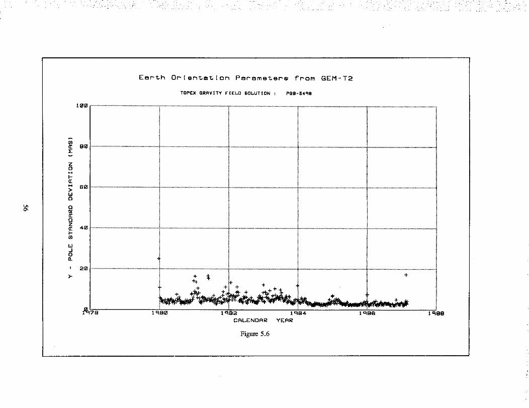
Ear_ch Or'[enZ._c[on Par'_me_cems fr-om GEM-T2

TOPEX GRRVITY FIELO BOLUTION : PGS-54qB

E 8_ ..........................................................................................................................................................................................................................................................................................................................

z i io i

$0 ................................................................:...............................................................................................................................:.............................................................................................................................>WO

Oo_ np

rrOZE 421 ...............................................................................................................................................................................................................................................................................................................................

W_I0n

' 20 ...........................................................................................................................................................................................................................................................................................................................

+ , �i+ +i + + 4- ":

4- 4- " 4" ++'E

_'I_178 IclSN I q82 Iq84 Iq86 Iq88

CF_L.ENDF_R YEFIR

Figure 5.6

Eer_h Orlen_m_lon ParBmeter8 £rom GEM-T2

TOPEX GRRVITY FIELO 80LUTION _ P86-54qB

I...................................................................................................................................................................................................................................................................i.................................................................Z0

M

_ 6 ................................................................................................................................................................................................................................................................. ° ......... , ......................... . ...........................

W0

M N

oZ

4 • • '

P

' I

d ................................................................ i

�i_+ +_, _ _,

.

l_7B lqBB lqB_ lqB4 lq:86 IqBBCALENDAR YEA_

Figu_ 5.7

Emr'lch Or-lenl;mt Ion Par_amelcer_s f'r-om GEM-T:>

TOPEX GRRVITY FIELD 60LUTION : PP_i_-54q@

E£

H

ivo _- + Eol_ --,- +_ -,-.+ _ . + i

,_..-_w-+....+.......... ±:_p..._.._....+...............+"_"z": ......................................................................._................................................................1

t++_ . i + + @+ • !W : + " +." ':_] - 10 ................................................................_.........±..................................................."...............................................................'=-..............................................................=-................................................................0 +nI

x .H-

.3bJ -_0 ...........................................................................................................................................................................................................................................................................................................................o +

CR_ENDRR YERR

Figu_ 5.8

886; 986I _e61 _86_ 886_ 8L__

0.......................................................................................................................................................................................................................................................................................................................... _ - IT]

[--

3)

-<!

"00

I'1

+. _ + : ,+ i_ _.+++,:.........................._'_L..........................-".............................._'........................:......._'"'_'_-_*.................................:"_""_"'"_+_................._":.............................................................._:

- + - , _ +4- i +

|

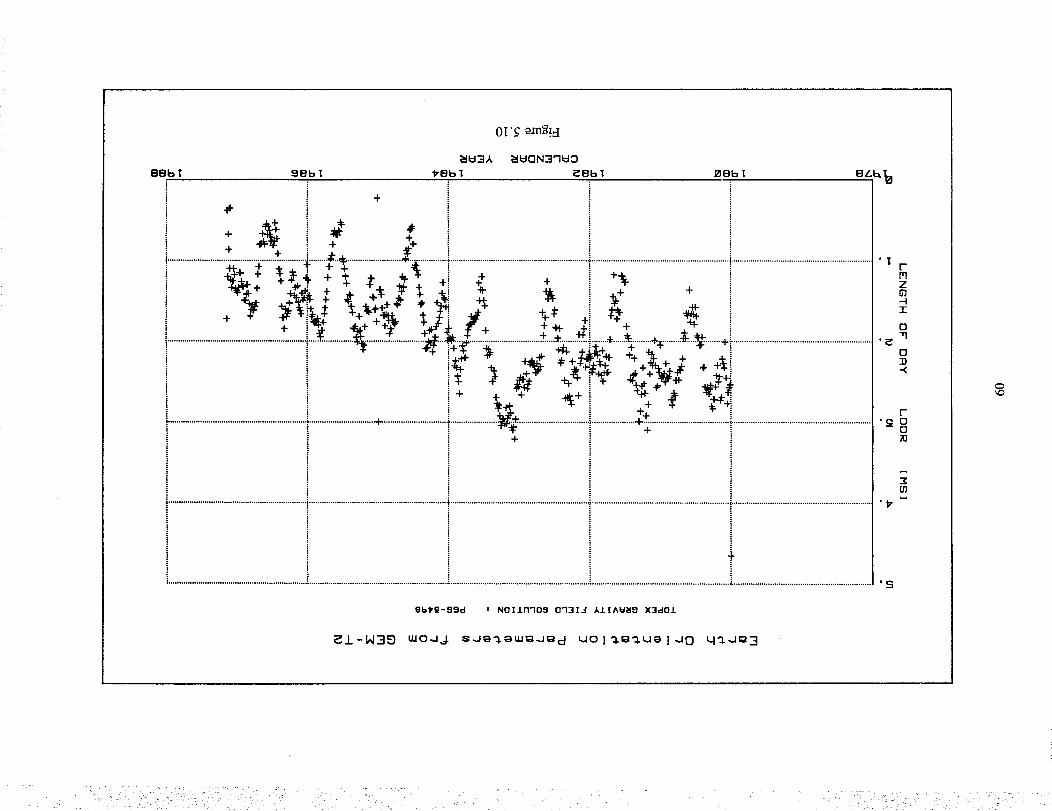
_II::I3A _II::I0 N3'-II::I 0

886 Z 886 _ 1,86 _ _86 "_ 886 _ 8L6,_

J +

+ "_ i + _i+

..................................................................i...._.............._........._.............._..4_..+...................................+......+........_i.......+......_.........+_......._..._.......+.................................................................g ,1€_ . +"4-_!¢,. _ _ i o

i _._ ++ _ __+.: [--

................................................................................................ �.............................._......................_ ................................_...................._._........................................................................................................_oo+ _0

U)

+

gb_g-88cl * NOI.Ln"IOS 0"1313 AIIA_I_IB X3c101

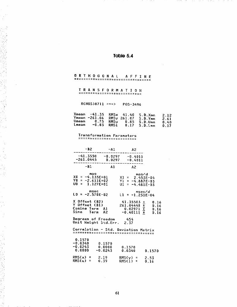
i_;ii̧

• Table 5.4

: ORTHOGONAL AFFI NE

TRANSFORMATION

R(NGS)8711 ===> PGS-3496

Xmean -41.35 RMSx 41.40 S.D.Xmn 2.12Ymean -261.06 RMSv 261.07 S.D.Ymn 2.61Umean 0.75 RMSu 0.85 S.D.Umn 0.40tmean -0.03 RMS1 0.17 S.D.Lmn 0.17

Transformation Parameters

-B2 -A1 A2

-41.3550 -0.0297 -0.4011-261.0445 0.0297 -0.4011

: -BI AI A2i

mas mas/dXO = -4.135E+01 XI = 2.453E-OqYO = -2.611E+02 Y1 = -4.887E-03UO = 1.127E+01 U1 = -4.q81E-03

msec msec/dLO = -2.570E-02 L1 = -1.251E-Oq

X Offset (B2) 41._550S + 0.16Y Offset (BI) 261.04448 ¥ 0.16Cosine Term A1 0.02971 + 0.16Sine Term A2 -0.40111 + 0.16

Degrees of Freedom _5_Unit Height _d. Err. 2.37

Correlation - Std. Deviation Matrix

0.1570-0.0340 0.1570-0.0243 0.0000 0.1570

0.0000 -0.0243 0.0340 0.1570

RMS(x) = 2.19 RMS(y) = 2.53RMS(u) = 0.39 RMS(1) = 0.16

61

transformation parameters indicated that there is no significant center of mass disagreementbetween these two modern reference frames; the orientation parameters which were estimated are

• _ as expected from the difference in polar motion and UTI origins between TOPEX/Poseidon "zero-mean" and BIH terrestrial origins. The center of mass offset in both x and y are significantly., s

..: _ different from zero, being around 30 em. It should be noted that the geocentricity of the Doppleri, Network is not guaranteed to correspond to that of the lasers; the lack of survey ties preclude

direct intercomparison. For example, any systematic effect on the network determination due to, ....., higher order ionospheric effects could manifest itself In the same way In both WGS-84 and the

_; GEM-T2 adjustments. However, we believe that these discrepancies are probably at the sub-meter level. Also of note, the earlier problems we have observed with DMA coordinates in the Zdirection have greatly diminished with these recent solutions.

Table 5.5COMPARISON OF GEOSAT GEM-T2 TRANET DOPPLER COORDINATES

'i WITH DMA/HTC SMTP WGS-84 COORDINATES

_: RMS OF FIT FOR 47 MATCHING STATIONS

!_ _ Earth Fixed: Geodetic Coordinates

, X 46 em Geodetic Latitude 0.014 arcsec

<

Y 42 cm Longitude 0.021 arcsee

Z 41 cm Spheroid Height 39 cm'i

TRANSFORMATION PARAMETERS

Center of Mass Rotation about Axis* Scale

X 30 ___8 cm X 0.266 - 0.03 arcsee 0 ± 12 partsper billion

Y -25 _ 8cm Y 0.046-+ 0.03 aresec

Z -5 ___8 cm Z 0.039 - 0.03 arcsec

* Expected Rotations from origin differences:

about X 0.280 arcsec

about Y 0.038 arcsec

63

• SECTION 6. THE DETERMINATION OF OPTIMAL DATA WEIGHTS" AND THE CALIBRATED ACCURACY OF GEM-T2

/

;: Determining optimum data weights and producing a reliable error model are now part ofan automated iterative procedure which has been employed in GEM-T2's development for the

, first time. This approach, as described in Lerch (1989), allows a new ease in the determinationof data weights and provides a calibrated error model as an integral part of the method. Prior

:i to the introduction of this approach, optimal data weighting was obtained from experimental:: solutions which were tested against orbital tracking data and independent gravity anomaly blocks

until no further improvement was seen in model tests. The top rated model was adopted and itsuncertainty was then calibrated after the fact to assure its reliability. Our experience has shownthat these models both performed well and were well calibrated although the method wasarduous. Calibration of model errors has historically been a complicated and time consumingundertaking. The techniques which were used to verify the models and calibrate theiruncertainties have evolved. The most recent attempts directly laid the foundation for thedevelopment of our new automated procedure. In general, they consisted of three types of tests

::: which are reviewed here since method Ca) is associated with the development of the optimal_: weighting algorithm presented in Section 4. The gravitational field calibrations which have been

:. used are:

(a) Calibration tests which compare the differences In the coefficients between twosolutions with the expected value of these differences using the solution error covariances. Thismethod has been extensively utilized with GEM-T1 tn comparison with versions of this modellacking specific data subsets.

(b) Calibration tests which compare the eigenvectors of these subset solutions in a fashionwhich parallels that used in method (a) but which is extended to include the off-diagonalcontributions in the error covariances.

(c) The oldest method (which has been used for over 15 years) is to compare the harmonic: gravitational models with independent gravity information. Since GEM-T1 and GEM-T2 are

"satellite-only" models, their results can be compared to the gravitational signal directly measured" by surface gravimetry or the gravity anomalies inferred from satellite altimetry. In the past, other

tests using satellite deep resonance passages, the longitudinal acceleration of synchronoussatellites, and tests on new sets of tracking data have provided the basis for these tests.

In method (a) the calibration test is essentially given in equation (4.14). This method hasbeen refined to separately test the spectral components of the gravitational models by segregatingthe results into constituents of a given degree, kt(1), and order, kt(m). Balanced solutions withproper data weights were found to calibrate well in general for any degree or order. Method (b)has not been employed as yet on GEM-T2 although it was found to give comparable results tomethod (a) for GEM-T1 (Lerch et al., 1988). Results for GEM-T2 are also given later in this

: section for method (c). Method (c) confirms that the calibrated error estimates of GEM-T2 as

obtained from our optimum weighting algorithm are highly reliable as demonstrated with testsagainst independent altimeter-derived gravity anomaly blocks.

:: PRECEDING PAGE BLANK NOT RIddED

,!

65 _.,,,IN II_Ntlgllllll,t,tl

6.1 Computations of Optimum Weights for GEM-T2',ij

_' Ji ,j

Using the weighting algorithm of Section 4.1 we show in Table 6.1 the preliminary subset,i _:! and complete solution calibrations based on the factors, k t, and weights I, W t obtained over• ! successive iterations. The subset solutions are obtained by deleting each of the major data sets

/ ,ii listed in the first column of this table from the complete solution. The first solution, PreliminaryGeopotential Solution (PGS)-3429 used initial data weights which were obtained in two ways.

....._'i • The apriori weights for PGS-3429 were based on the weights obtained in GEM-T1 as shown in• Table 4. la. For the data sets not included in GEM-TI (Table 4. lb}, initial weights were obtained

::_ by testing a solution which combined GEM-T1 with each of these new data sets individually:_ against GEM-TI itself, where in this case, GEM-T1 is the subset solution. We then applied the

weighting algorithm from equations (4.14) and (4.15) to converge on a set of weights for all of thei_ data which was previously not part of GEM-T1. This approach produced a set of apriori weights

i:_: for all of the major data sets of GEM-T2. This is the set of PGS-3429 data weights presented in: the third column of Table 6.1.

A set of subset solutions was computed for PGS-3429 where each of the major data setswas individually omitted from this preliminary version of GEM-T2. A set of calibration factors,

Kt, were obtained which are listed in the second column of Table 6.1. The initial calibration!,

factors indicated that these preliminary weights were quite reasonable. In Table 6.1 thecalibration factor (K t) scales the errors of the gravity parameters instead of the variances of theseerrors as given by k t, hence the values shown are:

K t = kt '/2

for the calibration factors in the table. The Kt calibration factor is more appropriate forexamining the convergence since its stability and sensitivity directly reflect the errors instead of

: their variances.

The weights on the data were then adjusted using equation (4.15) for the data sets wherei

Kt significantly differed from unity (shown as the underlined values) producing the values for thenext iteration of GEM-T2 which was PGS-3454. The procedure of computing subset solutions wasrepeated and a new set of calibration factors was obtained. These are shown in the fifth columnof Table 6.1 and they are noticeably closer to unity as compared to the factors obtained with PGS-3429. The process was again iterated, where new data weights were again computed and PGS-

' 3480 was solved using these values. The process of computing subset solutions was againrepeated and new calibration factors were derived. These are shown in the sixth column of Table6.1. Based on the calibration factors of PGS-3480, a new set of data weights for select data sets

: was determined which produced the GEM-T2 model. These Wt values are shown in the eighthi : column of this table. Subset solutions for GEM-T2 were computed and yielded the final set of

! calibration factors presented in the final column of Table 6. I. All of these values are acceptably

close to unity and the optimal weighting method has converged. It is desirable that Kt convergeto values slightly less than one in order to be conservative in the error estimation of thegeopotential field. For the case of the GEOS-3/ATS-6 data, the data weight was reduced givinga value of K t which was deliberately held at a conservative value because this data degraded the

_' model's performance when tested against independent data.

I The a's of unit weight are: 1 meter for range data, 1 cm/s for range-rate data and 2 seconds ofarc for camera data.

I

i!

i 66

? '

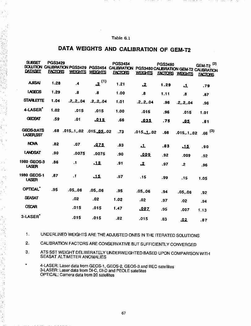
':" Table 6.1i

DATA WEIGHTS AND CALIBRATION OF GEM-T2

::::' i_ SUBSL=T PGS3429 PGS3454 PGS3480 GEM-T2 121. ,.;:_ _ CAUBRATIONPGS3429 PGS3454 CAMBRATION PGS3480 CAUBRATION GEM-T2 CALIBRATION:,il _TASSr _ WBGHm_ F.ecrc_s WEIGHTSF,_CrC__

• i AJISAI 1,28 .4 .3 (11 1.21 .2 1.29 .1 .79

.... _ 1.29 .8 .8 1.00 .8 1.11 .8 .87

• STA/:g.ETrE 1.04 .2,.2,.04 .2,.2,.04 1.01 .2,.2,.04 .96 .2o.2,.04 .96

4°LASER ° 1.02 .015 .015 1.00 .015 .96 .015 1.01

GBDI_T .59 .01 .015 .66 .035 .75 .05 .81

(3)GEOS_:ATS .68 .015,. 1,.02 .015,.05..02 .73 .015,J.,.02 .66 .015,.1 ,.02 .66

NOVA .82 .07 .075 .83 .1 .83 _15 .90

_T .90 .0075 .0075 .90 ,009 .92 .009 .92

1980 GEOS-3 .86 .1 .15 .91 .2 .97 .2 .96

,. 1980 GEOS-1 .87 .1 .15 .97 .15 .99 .15 1.05

OPTICAL* .95 .05,.06 .05,.06 .95 .05,.06 .94 .05,06 .92

SEASAT .02 .02 1.02 .02 .97 .02 .94

_ .015 .015 1.47 ,..007 .95 .007 f.13

:_ 3-LASER* .015 .015 .82 .015 .83 _ .87'i

1. UNDERLINED WEIGHTS ARE THE ADJUSTED ONES IN THE ITERATED SOLUTIONS

2. CALIBRATION FACTORS ARE CONSERVATIVE BUT SUFFICIENTLY CONVERGED

3. ATS SST WEIGHT DELIBERATELY UNDERWEIGHTED BASED UPON COMPARISON WITHSEASAT ALTIMETER ANOMALIES

, * 4-LASER: Laser data from GEOS-1, GEOS-2, GEOS-3 and BEC satellites. 3-LASER: Laser data from DI-C, DI-D and PEOLE satellites

..... OPTICAL: Camera data from 20 satellites

i

67

In general, the weights have converged for GEM-T2. One interesting fact about its subseti:i :::.i solutions is their good overall level of performance when tested against surface gravity anomalies

and test satellite orbital ares. Unlike GEM-T1, we find that the subset solutions for GEM-T2 all:ii perform nearly as well as the complete model itself on these independent tests. This is also true:,, ::: for the prediction of TOPEX/Poseidon's radial orbital accuracy. Hence this indicates that no

individual data set dominates the GEM-T2 solution which was not found to be the case to the_ :i same degree in GEM-TI.

' . This method assures a self-consistent set of data weights. This means that the model! changes predictably based on the solution error covariances given these weights when data is

:? removed from the solution. If this is so, then we are properly characterizing the data contributioni to the solution's accuracy and the resulting error covarlance should be calibrated and contain a: realistic estimate of solution uncertainty. This is tested in the next section where GEM-T2 is

calibrated with the independent global gravity information provided by altimeter-derived gravityi anomaly blocks.

• In practice, the gravitational models are also subjected to other tests using independentdata (method (c)). Weights on certain data sets may again be adjusted if a specific data setseems to produce results which conflict with independent data. In such a case, a data set maybe down weighted. As noted above, this was found to be the case and was used to downweight

• the contribution of the ATS-6/GEOS-3 SST observations in GEM-T2. These observations werei i

found to degrade the testing of the model against independently measured altimeter-deducedgravity anomalies. This calibration is discussed in the next subsection.

6.3 Calibration of GEM-T2 with 5° x 5° Mean Gravity Anomalies from Altimetry

Altimeter-derived gravity anomalies were also used to calibrate GEM-T2. Since theprevious methods indirectly test a field by comparing it internally to its data contributions, a

" possible concern is that both the full and subset solutions share a common systematic errorwhich would be untested using this method. The direct calibration of the model with independentand globally distributed altimeter gravity anomalies was undertaken to avoid this problem.

Mean 5° x 5 ° gravity anomalies are somewhat commensurate in field resolution with theharmonic model of GEM-T2. The values we are using here were computed from the 1° x 1° valuesdeveloped from the SEASAT and GEOS-3 Missions which were kindly provided to us by Rapp(1986). The gravity anomaly calibration was performed using the method given in Lerch et al.,

• (1988) for GEM-TI. Herein, we also corrected the altimeter anomalies using the high degree andorder gravitational field of Rapp and Cruz (1986) to remove contributions to the Ag values for allterms extending to degree 300 which are neglected from the GEM-T2 solution. The calibration

.... factor obtained from this comparison is given as:

k=( _ kt2 )V21066

:: (6.1)

where k I is an individual calibration factor computed for each of the 1066 5 ° blocks as:

]Ag -Age] lki -- .............................

[ o2(Ag) + o2(Age) ]'/2

{6.2)

68

and Ag and Age are the observed and GEM-T2 -computed gravity anomalies. When computing thegravity anomalies from GEM-T2 we used the spectral smoothing operator of Pellinen (Jekeli and

(!_ Rapp, 1980). The gravity anomaly uncertainties are obtained from the altimeter analysis of Rapp(1986) and GEM-T2 models respectively. The typical accuracy estimate for a 5° block predictedfrom GEM-T2 is 3.5 regals whereas those obtained from altimetry have accuracies in the 0.5 to

i 1 mgal range. Therefore, one can (in the extreme) assume that the altimeter anomalies areperfect, with little resulting change in the computed calibration factor for the tested gravity field.

i!_ As a consequence, this test is especially strong for it is insensitive to the accuracy assessment forthe independent data so long as o(Ag) << a(Agc). The global calibration factor obtained forGEM-T2 from this analysis is:

k = 0.98

ii i which indicated a high level of calibration consistency and gives an independent demonstrationof the values of the semiautomated calibration/data weighting approach.

Table 6.2 summarizes the GEM-T2 calibrations and demonstrates the performance of thesubset solutions when tested against these altimeter anomalies. Therein, one sees the RMS Agresidual between the gravitational field and the altimeter anomalies. Also shown is the covarianceprediction of global geoid error and the final calibration factors for the data subsets in GEM-T2.

: Quite encouragingly, each data subset made a positive contribution towards better resolving thegeoid through a statistical prediction (which is expected) as well as improving the agreement ofthe model when tested against altimetry.

, , , _ •' i ¸

i_ Table 6.2i

_:,_ Summary of Calibration Factors for GEM-T2 Using Subset Solutions_:, and Other Measures of Subset Field Performance

i i Data Subset Kt Estimated Comparison.... Omitted from (Overall Calib.) Geoid Ht. with Altim

GEM-T2 Factor Error (m) Grav. Anom.

(mgals**2)i I

ii none .... 140.5 12.5

!!i

i: Aj isai 0.79 141.3 12.6

' GEOSAT 0.81 145.8 12.9L:

NOVA- 1 0.90 146.2 12.9

Peole, D1D, D1C 0.87 159.0 12.8

Lageos 0.87 141.4 12.6

pre-1980 GEOS 1,2,3, 1.01 146.2 13.6BEC

.: i Oscar 1.13 141.1 12.6

Starlette 0.96 150.2 14.1

SEASAT 0.94 141.1 12.7

: Landsat 0.92 142.8 12.7

1980 GEOS-1 1.05 141.3 12.5

1980 GEOS-3 0.96 143.2 12.6

Optical Data 0.92 147.1 13.5

GEOS-3/ATS-6 SST 0.66 140.7 12.5• J

,ii

70

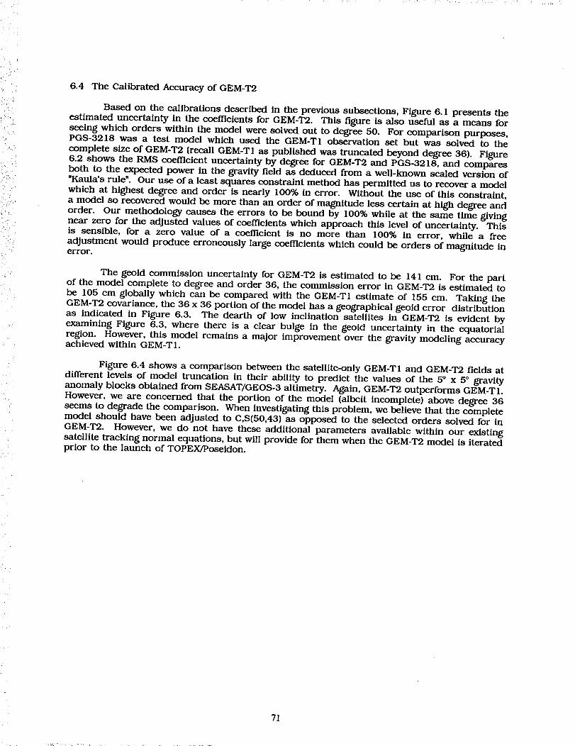
6.4 The Calibrated Accuracy of GEM-T2

Based on the calibrations described in the previous subsections, Figure 6.1 presents the_ _ estimated uncertainty in the coefficients for GEM-T2. This figure is also useful as a means for

_'_i: seeing which orders within the model were solved out to degree 50. For comparison purposes,PGS-3218 was a test model which used the GEM-T1 observation set but was solved to the

: complete size of GEM-T2 (recall GEM-T1 as published was truncated beyond degree 36). Figure6.2 shows the RMS coefficient uncertainty by degree for GEM-T2 and PGS-3218, and compares

:i : both to the expected power in the gravity field as deduced from a well-known scaled version of• "Kaula's rule". Our use of a least squares constraint method has permitted us to recover a model

, ; : which at highest degree and order is nearly 100% in error. Without the use of this constraint,a model so recovered would be more than an order of magnitude leas certain at high degree and

i:,::_,,: order. Our methodology causes the errors to be bound by 100% while at the same time givingnear zero for the adjusted values of coefficients which approach this level of uncertainty. Thisis sensible, for a zero value of a coefficient is no more than 100% in error, while a free

....: adjustment would produce erroneously large coefficients which could be orders of magnitude inerror.

The geoid commission uncertainty for GEM-T2 is estimated to be 141 cm. For the partof the model complete to degree and order 36, the commission error in GEM-T2 is estimated tobe 105 cm globally which can be compared with the GEM-T1 estimate of 155 cm. Taking theGEM-T2 covariance, the 36 x 36 portion of the model has a geographical geoid error distributionas indicated in Figure 6.3. The dearth of low inclination satellites in GEM-T2 is evident by

.... examining Figure 6.3, where there is a clear bulge in the geoid uncertainty in the equatorialregion. However, this model remains a major improvement over the gravity modeling accuracyachieved within GEM-T1.

• Figure 6.4 shows a comparison between the satellite-only GEM-T1 and GEM-T2 fields at• different levels of model truncation in their ability to predict the values of the 5 ° x 5° gravity

anomaly blocks obtained from SEASAT/GEOS-3 altimetry. Again, GEM-T2 outperforms GEM-TI.However, we are concerned that the portion of the model (albeit incomplete) above degree 36seems to degrade the comparison. When investigating this problem, we believe that the completemodel should have been adjusted to C,S(50,43) as opposed to the selected orders solved for inGEM-T2. However, we do not have these additional parameters available within our existingsatellite tracking normal equations, but will provide for them when the GEM-T2 model is iteratedprior to the launch of TOPEX/Poseidon.

71

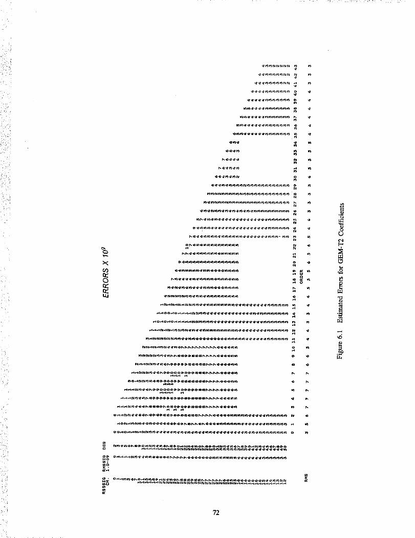
9ERRORX 10

8GEM-T1' .7 x KAULA

,

t

Ip..._

1 /

._ GEM-T1'= GEM-T1SOLVEDTOGEM-T2SIZE• . , I, I L, • • • I • • m • I ' • _ ' ' I • ' " _ I ' I • _ I • • • • I " • • • I " • " " I " I

0 5 10 15 20 25 30 35 40 45 50

Figure 6.2 RMS of Coefficient Errors Per Degree

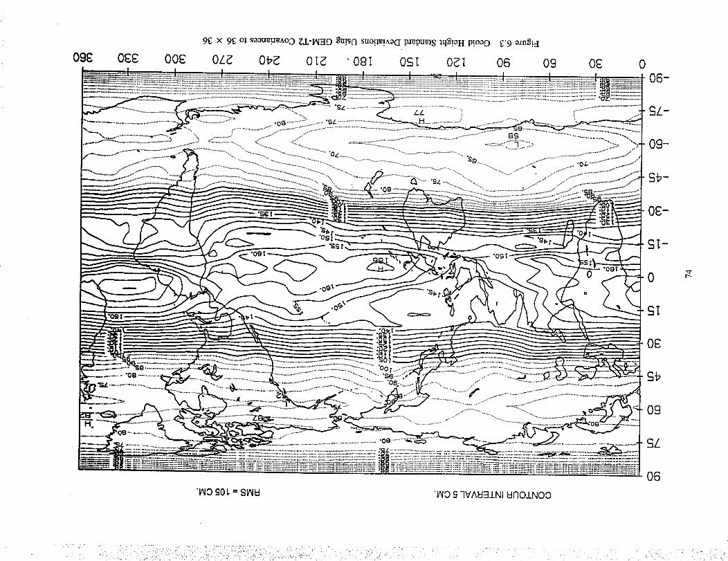
9E X 9£ O:1.SOoT.re.T_AO_) _,.L-I,_:';ID _'U.lSl'l SUO.EI.I_.IAO(Ip.I_pLmlS lq_.tOH pT.ogo t;'9 o.In_.t4

09_ OE£ OOE OL_ 0_'_ 0I_ '08I OS_ 0_I 06 og OE 0I:.............:_..........I L 06-

"_ .................7';...........................i SL-....................... '";-' "Og .............:_' ......"_/--" '--_[....... "

• - .......... ................. .................................................. _

..........................':......... :::........ '............'."::::::L...7 ,,::::::,:"7_"'i;:::.: Og"

...........................'................. ......................'............o,_....... '...................................................._; ........" ............. '............ ' .................. _ ...... oz, ............................

......,"',,_

._.......... i--..... S_-,., ......................... ...."

•_ Og-

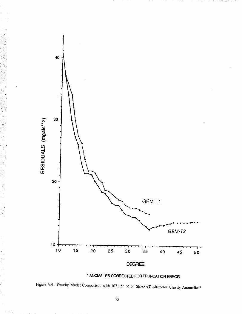
GEM-T2

10

10 15 20 25 30 35 40 45 50

DEGREE

° ANOMALIESCORRECTED FOR TRUNCATION ERROR

Figure 6.4 Gravity Model Comparison with 1071 5 ° × 5 ° SEASAT Altimeter Gravity Anomalies*

75

, :(

: -, SECTION 7. ORBIT ACCURACIES FOR GEM-T2i

i>,,i: One of the principal demands made of terrestrial gravitational models is to accuratelyi_ represent the conservative forces acting on Earth-orbiting satellites. The requirements for precise

orbit modeling are an important element in the success of many geodetic missions. This includes

..... satellites designed to monitor the Earth's tectonic motions like LAGEOS and those requiringaccurate radial positioning of an altimeter bearing satellite to locate the ocean surface in a

:; geocentric reference frame like SEASAT and TOPEX/Poseidon. GEM-T2 has been tested with<i_,.:! satellite tracking data acquired on a number of missions to assess its overall performance and:_:::, to compare it with other contemporary models.

• 7.1 Gravity Model Tests Using Tracking Observations

Table 7.1 displays a series of test orbital arcs spanning all of the satellites available forOur analysis which have modern precise laser and Doppler tracking. Compared therein, is theRMS of fit obtained on these test orbits for all of the recent "satellite-only" Goddard Earth Models

, produced over the last decade. Two important points are evident in these results. First, there< has been enormous progress in the accuracy by which we are able to model the conservative

forces arising from the static and tidal geopotential acting on near-Earth satellites, with GEM-T2' continuing this tradition. Second, there remains a significant gap in the accuracy by which we

are able to compute and thereby reconstruct an orbital history as compared to the inherentaccuracy of the data themselves. These test arcs were 5 to 6 days in length containing globallydistributed observations for all satellites with the exception of LAGEOS, where 30-day orbital arclengths were used.

Very significant improvement is seen in the modeling performance of Starlette and GEOS-.... :: 3 with GEM-T2. There are two factors which have contributed to these results. By extending the:, GEM-T2 model to include coefficients of 41st, 42nd and 43rd orders, GEM-T2 now models higher

order resonance effects which are especially significant on these two satellites. The general overallimprovement obtained with GEM-T2 is an additional contributing factor which is seen in the

• • overall orbit modeling improvement across these tests.

7.2 Radial Orbit Accuracy on SEASAT

The altimeter data taken by SEASAT enables us to isolate the radial modeling performanceof different gravitational fields on its orbit. This is possible by evaluating the difference in thealtimeter measured sea surface height at groundtraek crossover locations. Since the sea surfaceheight is approximately static given its conformance to the geoid (with small effects due tomesoscale sea surface variability and mis-modeled tides being present), the value of the seasurface height can be considered Ume-invariant. When the height of the sea surface above thereference ellipsoid at the same geographical point on the Earth's surface is measured by crossingaltimeter passes, the difference in the heights is a reasonably strong measure of the non-geographically correlated radial orbit error. This assessment of the radial error is not complete,for part of the gravity error contribution is geographically dependent yet it subtracts when formingthe crossover difference. Nevertheless, there remains the time-dependent radial error which iswell sensed by this method, although other errors can contribute to this difference at the 5- to

i, 20-cm level (i.e., mismodelled tidal and atmospheric refraction corrections, and mesoscalei_' oceanographic effects).

Table 7.2 shows a comparison on six test SEASAT ares, three of which were taken when' SEASAT was in a 17-day repeating groundtrack configuration, the others when SEASAT was in

a 3-day repeat. TRANET Doppler data from a global network of stations was the only data used: in the orbit adjustment process. These orbits were then passed through the independent altimetry

and an assessment of the crossover misclosure was obtained. Four fields are compared withinTable 7.2:

i

77

,) op,

Table 7.1

Orbit Accuracy Assessments ofSatellite Fields Using Test Arcs

(rms of fit)

GravityField LAGEOS AJISAI STRLT BE-C GEOS1 GEOS2 GEOS3 NOVA

(m) (m) (m) (m) (m) (m) (m) (cm/s)GEM-9 (1979) .333 .951 1.16 .873 1.26 1.18 1.72 0.95GEM-L2 (1981).199 .797 1.00 .893 1.07 1.09 1.87 0.79GEM-T1 (1987) .069 .181 .172 .396 .387 .655 .693 0.44GEM-T2 (1989) .066 .151" .102 .334 .316 .667 .249 0.37*

NOISE

FLOOR .038 .038 .040 .102 .206 .343 .101 .335

* Satellitenowin model

Ca) PGS-S4 (Lerch et al., 1982a) was a "tailored" gravity model which used SEASAT laser,_ S-Band range-rate and altimeter data which for its time, was the state-of-the-art for SEASAT

precise orbit determination. This gravity field was used for the Geophysical Data Records toproduce the orbital information for the distributed data. By using SEASAT altimetry, this modelwould be expected to perform quite well on SEASAT, and did reduce the radial modelinginaccuracies on this trajectory from the 2-4 meter level to that of _ 75-cm,

(b) GEM-TI (Marsh et al., 1988) was a "satellite-only" model which utilized SEASAT_i TRANET and laser observations. It contained no altimetry, but does contain the considerable

.... improvement which was accrued in our efforts to improve the models for TOPEX/Poseidon.

(c) GEM-T2 is the new GSFC "satellite-only" model described in this report whichcontained the same SEASAT observation set as that of GEM-TI. Any improvement in the SEASATperformance is therefore, a direct result of improving the general gravitational field.

: (d) PGS-3337 (Marsh et al., 1989) is a preliminary combination model complete to degreeand order 50 which utilizes GEM-TI's tracking data with surface gravlmetry and SEASATaltimetry. Unlike PGS-S4, this model now simultaneously solves for a harmonic model of the

i dynamic sea surface height which causes the sea surface to depart from the geoid at the 60-70-cm level.

.... Table 7.2 shows excellent results for GEM-T2 which exceed those found in GEM-T1 bya considerable amount. These models are certainly superior to that achieved with PGS-S4although this latter model used the SEASAT altimeter data directly. As a point of interest, theGEM-T2 error covariance matrix predicts 19 cm for the radial accuracy one should obtain fromthis field. The prediction for GEM-T1 is 44 cm.

7.3 Projected Orbit Errors Due to Static Gravitational Modeling Uncertainties

The error covarlance matrix can be used to project the gravitational modeling error ontoany orbital configuration. This projection uses the first-order analytical perturbation theorydeveloped by Kaula (1966) and gives a harmonic estimate of modeling error. This estimate doesnot take into account the distribution of tracking data nor does it consider the additional errorarising from the erroneous estimation of the orbital state (epoch) position which propagates with

• the well-known "once-per-revolution" orbit errors commonly seen in data analyses. However, withthe distribution of modern tracking networks and the typical performance of these trackingsystems in their support of numerous missions, we have found through comparisons withnumerical tests and data simulations, that these first-order projections are quite reliable inmapping a given gravity error into orbit error overall.

For these projections, we have developed an additional preliminary gravitational field.PGS-3520 (Marsh et al., 1989} is a combination model which is similar in design to that of PGS-3337. It is a model complete to degree and order 50 which utilizes tracking observations, surfacegravimetry and SEASAT altimetry. Unlike PGS-3337 which relied on the tracking data used informing GEM-T1, PGS-3520 is based on GEM-T2. Unlike GEM-T1 and GEM-T2, this combination

• model has not been extensively calibrated, and it is only Introduced herein to give some indicationof what a GEM-T3 model is likely to do in gravity modeling performance. GEM-T3 will use nearly

::_ all of the data available for gravity modeling improvement, and therefore PGS-3520 can give atleast a preliminary estimate of what the total yield from historical data is likely to be.

Table 7.3 presents the projected orbit uncertainties in the radial, along-track and cross-

_,:i_i_ track (normal} ballistic components for many existing and to-be-launched satellites. It comparesthe projected performance of GEM-T1, GEM-T2 and PGS-3520. For the TOPEX/Poseidon orbit

.... in specific, these estimates indicate that we are approaching the level of modeling required to

!i support this mission's radial error budget. Figure 7.1 presents a radial orbit uncertainty!_ projection for a satellite at the nominal altitude of TOPEX/Poseidon (1341 km) using the GEM-, T2 eovariances for different orbital inclinations. For comparison purposes, also shown are the

79

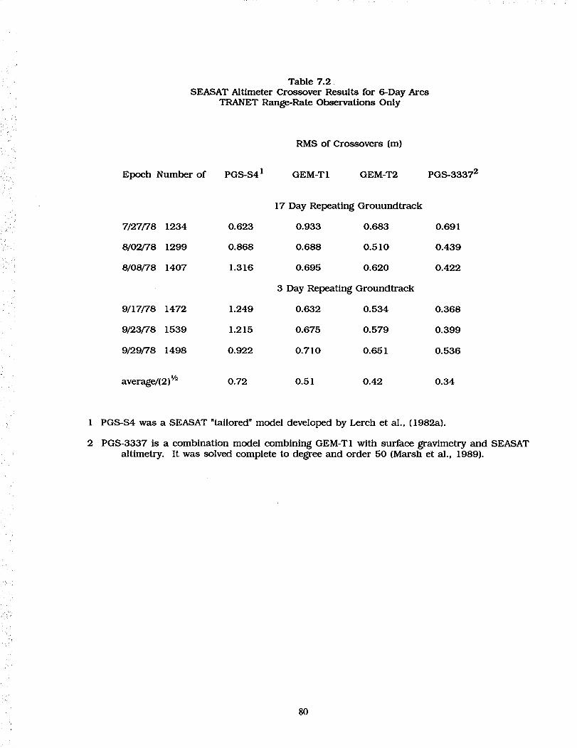
Table 7.2

SEASAT Altimeter Crossover Results for 6-Day ArcsTRANET Range-Rate Observations Only

•,

RMS of Crossovers (m)

Epoch Number of PGS-S41 GEM-TI GEM-T2 PGS-33372

17 Day Repeating Grouundtrack. ! '

ii!i 7/27/78 1234 0.623 0.933 0.683 0.691

_ i 8/02/78 1299 0.868 0.688 0.510 0.439

8/08/78 1407 1.316 0.695 0.620 0.422

3 Day Repeating Groundtrack

9/17/78 1472 1.249 0.632 0.534 0.368

9/23/78 1539 1.215 0.675 0.579 0.399

9/29/78 1498 0.922 0.710 0.651 0.536

i

average/(2) I/2 0.72 0.51 0.42 0.34

_ I PGS-S4 was a SEASAT "tailored" model developed by Lerch et al., (1982a).

2 PGS-3337 is a combination model combining GEM-T1 with surface gravimetry and SEASATaltimetry. It was solved complete to degree and order 50 (Marsh et al., 1989).

8O

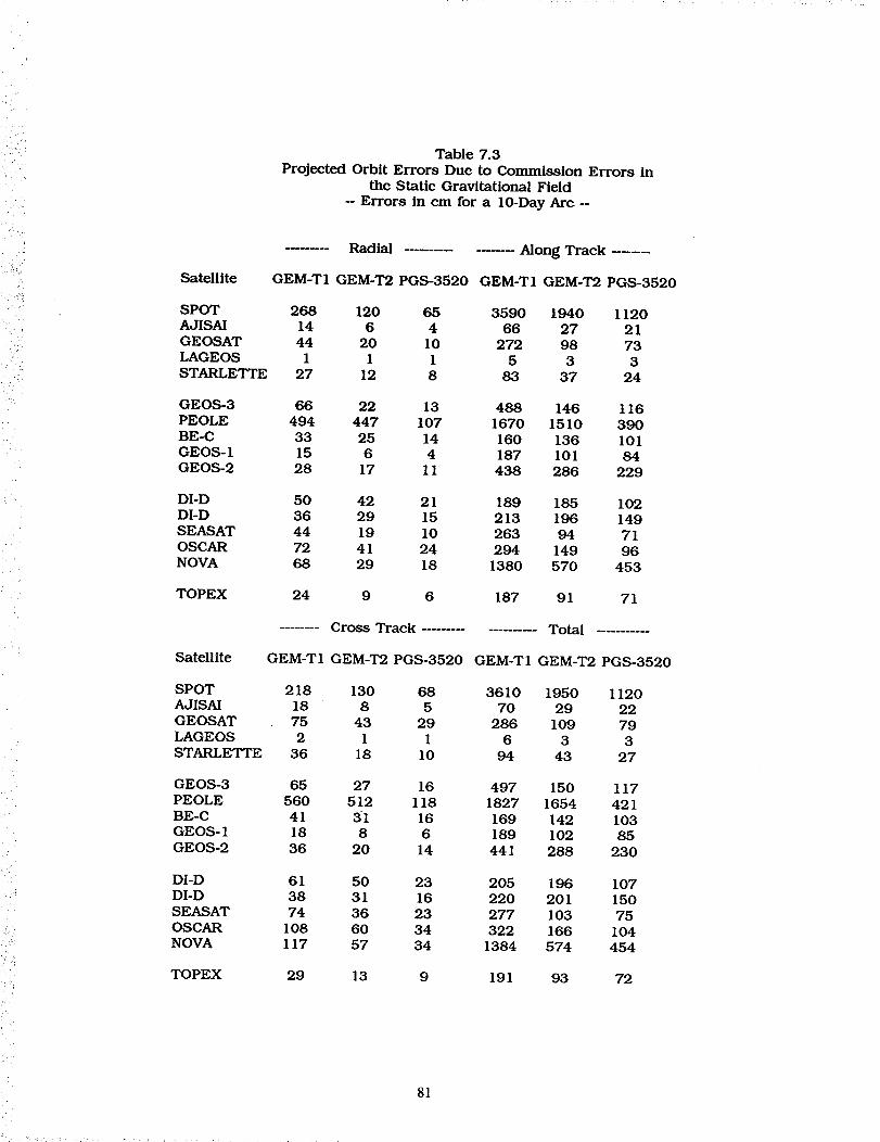
Table 7.3Projected Orbit Errors Due to Commission Errors in

the Static Gravitational Field

-- Errors in em for a 10-Day Are--

......... Radial ................. Along Track ........

_ Satellite GEM-T1 GEM-T2 PGS-3520 GEM-TI GEM-T2 PGS-3520

SPOT 268 120 65 3590 1940 1120AJISAI 14 6 4 66 27 21

• GEOSAT 44 20 10 272 98 73'i_! LAGEOS 1 I I 5 3 3

_ STARLETTE 27 12 8 83 37 24

GEOS-3 66 22 13 488 146 116PEOLE 494 447 107 1670 1510 390BE-C 33 25 14 160 136 101GEOS-I 15 6 4 187 I01 84GEOS-2 28 17 11 438 286 229

DI-D 50 42 21 189 185 102DI-D 36 29 15 213 196 149SEASAT 44 19 I0 263 94 71OSCAR 72 41 24 294 149 96NOVA 68 29 18 1380 570 453

TOPEX 24 9 6 187 91 71

........ Cross Track ................... Total ...........

Satellite GEM-T1 GEM-T2 PGS-3520 GEM-T1 GEM-T2 PGS-3520

SPOT 218 130 68 3610 1950 1120AJISAI 18 8 5 70 29 22GEOSAT 75 43 29 286 109 79LAGEOS 2 1 1 6 3 3STARLETTE 36 18 I0 94 43 27

GEOS-3 65 27 16 497 150 117PEOLE 560 512 118 1827 1654 421BE-C 41 31 16 169 142 103GEOS-1 18 8 6 189 102 85GEOS-2 36 20 14 441 288 230

DI-D 61 50 23 205 196 107i DI-D 38 31 16 220 201 150

SEASAT 74 36 23 277 103 75OSCAR 108 60 34 322 166 104NOVA 117 57 34 1384 574 454

TOPEX 29 13 9 191 93 72

81

projections for GEM-T1 and PGS-3520. The large improvement seen at 65.5 ° inclination betweenGEM-T1 and GEM-T2 is largely a result of the additional high-precision GEOS-3 observations

...... i added to GEM-T2 which are at this inclination. The satellite-only solutions are highly dependenton the inclination distribution of the data which is used to compute the model. Weak lowinclination data sets result in poor projected field performance for a satellite orbiting at an

::':! inclination of less than 35 ° (or greater than 145 °) when either GEM-T1 or GEM-T2 are used. The' sensitivity of the model uncertainties to orbital inclination are significantly reduced with the

introduction of altimeter and surface gravimetry into combination models. PGS-3520 showssignificantly flatter uncertainties than either of the satellite models. Figures 7.2 and 7.3 show the

i:i:iil gravitational modeling uncertainty of GEM-T1 and GEM-T2 projected on the radial component of: :_ the TOPEX/Poseidon orbit for terms grouped by degree and order respectively. Both of these_i:: figures indicate a broad general improvement in GEM-T2 which is found across the perturbation

spectrum of TOPEX/Poseidon's orbit. Of special interest is the improved modeling of thei i

::: resonance and m= 1 orders found with GEM-T2.

7.4 Discussion of the SEASAT Altimeter Crossover Results

An explanation is warranted to reconcile our prediction of GEM-T2's SEASAT radial orbit errorshown in Table 7.3 and the 59-cm (= 42 x 2 V2) RMS altimeter misclosure error shown in Table7.2. The first topic to address is the relationship of the 19-cm estimate to the crossovermeasurement. It is well known that altimeter crossover tests only detect part of the radial orbiterror--that part which is time varying and not the geographically correlated error. The 19-cmestimate in Table 7.3 is a combined value containing the total radial error. It has also been foundthat the error is approximately equally distributed between the geographically correlated error andthe time varying error globally. Therefore, one would expect only 14 cm coming from thecontribution of each are to the crossover discrepancy. We have performed a numerical simulationon SEASAT using GEM-T2 and a gravitational field ("clone") which is one standard deviation awayfrom GEM-T2. This experiment showed a 19.4 cm RMS radial orbit difference (which agrees verywell with our analytical prediction of 19 cm) in the orbits predicted by the two models; moreoverit was found that 14 cm was the time varying error which would be sensed in the crossoverresults, with the geographically correlated error contributing 14 cm. Rosborough (1986) hasshown that the time varying radial error maps by a factor of 2 into the crossover residuals giventhe changing sign of the geopotential error propagation into the ascending vs. descending track.Therefore, one would expect a 28 cm contribution from GEM-T2's errors in the crossovermisclosure. There are numerous other errors which enter into the crossover computation whichare described in Table 7.4. The total contribution from these errors accounts for an additional

24 cm in the crossover RMS. What remains to explain the 59-cm value obtained experimentallyfrom the real data are other sources of orbit error including the modeling of atmospheric drag,solar pressure, Earth albedo and the contribution of data systematics arising from the TRANETII tracking systems used to compute these orbits. Our analyses show that drag and solarradiation pressure errors on SEASAT are typically 15 cm over a 6-day arc. Therefore, solving

i the following equation and ignoring the small contribution from Earth albedo, we get:

592 = 282 + 242 + (15x2V2) 2 + X 2

where X = 41 cm and it represents the error in the orbit due to TRANET II being the onlytracking data used in the orbit's determination. The question which remains: Is this valuereasonable? Confirmation of this estimate can be found in Marsh et al., (1989a; Table 9) wherethe crossover RMS for PGS-3337 using Doppler data alone was 47 cm and 31 cm when altimetrytreated as tracking data was added to the solution. (472 - 312 )1/2= 35 cm which shows theimprovement obtained with the introduction of altimeter data. It is also clear to us that the useof altimetry has not eliminated all of the systematic errors (e.g., neglect of third-order ionospheric

.... refraction modeling, oscillator errors, station position errors, etc.) introduced in the orbitcomputation from the TRANET data, for these data are still being used. Also, the introductionof altimetry has its own error sources. Furthermore, from Table 4.1 it is shown that the "true"

value of the TRANET II observations in the gravitational field determination is represented by anoise estimate of 7cm/s as obtained in our optimal data weighting method. If one were to takethe noise-only uncertainty for the SEASAT orbit's radial component assuming 7cm/s Doppler data

t

82

20O

* PGS3520 = PGS3496 + S.G. + SEASAT ALTIMETERO

n" 150On"n"uJ_..I,,<a

oo <n-

100

PGS3496(GEM-T2)

GEM-TI

,o \

PGS3520"

• I I ' I ' I ' I ' I ' I ' I ' "' i ' ' I ' I " I • '1 '' ' I " I " I " I ' " I

0 10 20 30 40 50 60 70 80 90 100 110 120 130 140 150 160 170 180

INCLINATION (DEG.)Figure 7.1 Predicted Radial Error From Gravity Covariances 1341 Kin. Altitude

RMS PER ORDER

, 10-DAY ARCIIIIIII10 ,,IIIIIIIIII

II!I

P\ _ GEM-T1(TOTALRMS=24.1)8 '

I

I

_ \ ,mu_l , ,

6 i i\ ,z , __'_ l _I' ',,,,ii, I

I + ", 1I I !

, N 1 'I ! J

GEM-T2 ( TOTAL RMS = g.4 ) I

'I I I II I I III I I II I I II I I II I l II I I I

' ' iA';'I I I

I I t

_I II I _'_. ..¢I I ,II t,] "'----< I X'_

00 5 10 15 20 25 30 35 40 45 50

Figure 7.3 TOPEX Projected Radial Error

i. ¸

noise, the noise contribution would exceed 45 cm for each of the tested arcs._i

_ Nevertheless, the original estimate for GEM-T2's performance on SEASAT shown in Table.......,_ 7.3 assumed perfect orbit tracking information in all components; in this experiment with PGS-'J 3337, a 35-cm improvement is obtained through the introduction of restricted high-quality orbital.( _ radial information over the oceans. Our estimate of 35 to 40 cm is a realistic assessment of the...._ radial orbit error contribution coming from the exclusive use of Doppler tracking to produce the_ii results in Table 7.2. Therefore, we conclude that our overall error estimate for the gravitational

field's contribution to SEASAT shown in Table 7.3 is confirmed to be realistic and consistent with_ : other contributing error sources.

_..

. jl

Table 7.4i

Error Sources Contributing to Altimeter Crossover Misclosures on SEASAT'>'i

Error Source Approximate Magnitudei (cm)

...., Ocean/solid Earth I0tides

EM Bias 5

Data Noise (altimeter) 10

Media 5

Spatial Interpolation 2

Altimeter pointing/timing 2

Root Sum of Squares: 16

TOTAL: Two observations involved 241in crossover computation

1 Obtained by: 16 x 2 '/2, i

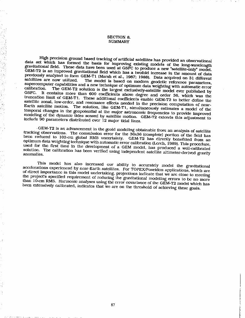
SECTION 8.SUMMARY

' L •

High precision ground based tracking of artificial satellites has provided an observationaldata set which has formed the basis for improving existing models of the long-wavelength

'_'_, gravitational field. These data have been used at GSFC to produce a new "satellite-only" model.'_ ii__ GEM-T2 is an improved gravitational field which has a twofold increase in the amount of data;_:_._ previously analyzed to form GEM-T1 (Marsh et al., 1987; 1988). Data acquired on 31 different

satellites are now utilized. The model is based on modern geodetic reference parameters,: ' supercomputer capabilities and a new technique of optimum data weighting with automatic error

calibration. The GEM-T2 solution is the largest exclusively-satellite model ever published by: GSFC. It contains more than 600 coefficients above degree and order 36, which was the:_i( truncation limit of GEM-T1. These additional coefficients enable GEM-T2 to better define the

satellite zonal, low-order, and resonance effects needed in the precision computation of near-_ Earth satellite motion. The solution, like GEM-TI, simultaneously estimates a model of the!': temporal changes in the geopotentlal at the major astronomic frequencies to provide Improved

modeling of the dynamic tides sensed by satellite motion. GEM-T2 extends this adjustment toinclude 90 parameters distributed over 12 major tidal lines.

•GEM-T2 is an advancement in the geold modeling obtainable from an analysis of satellitetracking observations. The commission error for the 36x36 (complete) portion of the field hasbeen reduced to 102-em global RMS uncertainty. GEM-T2 has directly benefitted from anoptimum data weighting technique with automatic error calibration (Lerch, 1989). This procedure,used for the first time in the development of a GEM model, has produced a well-calibratedsolution. The calibration has been verified using independent satellite altimeter-derived gravityanomalies.

This model has also increased our ability to accurately model the gravitationalaccelerations experienced by near-Earth satellites. For TOPEX/Poseidon applications, which areof direct importance in this model undertaking, projections indicate that we are close to meetingthe project's specified requirement of reducing the gravitational modeling errors to be no morethan 10-cm RMS. Harmonic analyses using the error covariance of the GEM-T2 model which hasbeen extensively calibrated, indicates that we are on the threshold of achieving these goals.

87

ACKNOWLEDGEMENTS

The authors would like to acknowledge the TOPEX/Poseidon Project at JPL for its support!,_ of our gravity modeling improvement activity. We also are thankful for the support this work is

: :_: receiving from NASA's Geodynamics Program.

Many individuals have provided valuable information and help in the development of

GEM-T2. Richard Rapp and Nick Pavlis of Ohio State University are to be thanked for their: _,_ analysis and evaluation of the surface gravlmetry. George Born and George Rosborough of the

_: University of Colorado have assisted us in improving our methods for calibrating the model. The:._ ,/ University of Texas' Center for Space Research under the direction of Byron Tapley has also:_/: played an important role as a sounding board for our activities.

" 88

:. REFERENCES

_': :

Anderle, R.J., "Doppler Satellite Data Characteristics," Naval Surface Weapons Center Document

;,:: TR 83-353, October 1983.2"

Bursa, M., "Geodynamcis Due to the Varying Second Zonal Geopotential Harmonic," paper: presented at the 26th COSPAR Conference, Toulouse, France, 1986.

Chao, B.F., W.P. O'Connor, A.T. Chang, D.K. Hall, and J.L. Foster, "Snow Load Effect on theii_ Earth's Rotation and Gravitational Field, 1979-1985," J. Geophys. Res., 92, B9, pp. 9415-

12

9422, 1987.

!_;i Chao, B.F. and W.P. O'Connor, "Global Surface-Water-Induced Seasonal Variations in the Earth'sRotation and Gravitational Field," Geophys. J., 94, pp. 263-270, 1988.

Chao, B.F., "Excitation of the Earth's Polar Motion due to Mass Variations in Major Hydrological,'_,: Reservoirs," J. Geophys. Res., 93, Bll, pp. 13811-13819, 1988.

• Christodoulidis, D.C., R.G. Williamson, D. Chinn, and R. Estes, " On the Prediction of OceanTides for Minor Constituents," Proceedings of the 10th International Symposium on EarthTides, edited by R. Vieira, pp. 659-678, Conseja Superior de Investigaciones, Madrid,Spain, 1986.

Christodoulidis, D.C., D.E. Smith, R.G. Williamson, and S.M. Klosko, "Observed Tidal Brakingin the Earth/Moon/Sun System," J. Geophys. Res., 93, B6, pp. 6216-6236, 1988.

Figgatte, C. and A. Polesco, "Laser Preprocessor Program User's Guide," Contract Report 5-24300, Task 769, Computer Science Corporation, June, 1982.

Goad, C., "A Modified Hopfleld Tropospheric Refraction Correction Model," paper presented atthe Fall Meeting of the American Geophysical Union, December 1974.

' Gross, J.E., "Preprocessing Electronic Satellite Observations," Ohio State Contractor's Report,NASA CR 1183, November 1968.

Gutierrez, R. and C.R. Wilson, "Seasonal Air and Water Mass Redistribution Effects on LAGEOSand Starlette," paper in press, 1988.

Hedin, A.E., "High Altitude Atmospheric Modeling," NASA Tech. Memo. 100707, Greenbelt, MD,October 1988.

Hotter, F., "Preprocessing Optical Satellite Observations," Ohio State Report 82, Columbus, OH,May 1968.

Jacchia, L.G., "Revised Static Model of the Thermosphere and Exosphere with EmpiricalTemperature Profiles," Special Report 332, Smithsonian Astrophysical Observ., Cambridge,MA, 1971.

Jekeli, C. and R.H. Rapp, "Accuracy of the Determination of Mean Anomalies and Mean GeoidUndulations from a Satellite Gravity Field Mapping Mission," Report No. 307, Departmentof Geodetic Science, Ohio State University, Columbus, Ohio, August, 1980.

,j

, Kahn, W.D., S.M. Klosko, W.T. Wells, "Mean Gravity Anomalies from a Combination of ApolIo/ATS6 and GEOS-3/ATS 6 SST Tracking Campaigns," J. Geophys. Res., 87, B4, pp. 2904-2918,1982.

Kaula, W.M., Theory of Satellite Geodesy, Blaisdell, Waltham, MA, 1966.

89

'iI : _/

i _i__!

:: Lereh, F.J., S.M. Klosko, R.E. Laubscher, C.A. Wagner, "Gravity Model Improvement Using GEOS-3 (GEM-9 and 10)," J. Geophys. Res., 84, 3897-3915, 1979.

_'!r,i

i:!_:i Lereh, F.J., J.G. Marsh, S.M. Klosko, and R.G. Wllltamson, "Gravity Model Improvement fori::_,_ SEASAT," J. Geophys. Res., 87, C5, pp. 3281-3296, 1982a.

: .... : Lerch, F.J., S.M. Klosko, G.B. Patel, "Gravity Model Development from LAGEOS," Geophys. Res._,_ _

, Letters, 9, pp. 1263-1266, 1982b.J

_, Lerch, F.J., "Error Spectrum of Goddard Satellite Models for the Gravity Field," GeodynamicsBranch Annual Report-1984, NASA Tech. Memo. 86223, Greenbelt, MD, August 1985.

__i_: Lerch, F.J., J.G. Marsh, S.M. Klosko, E.C. Pavlis, G.B. Patel, D.S. Chinn, and C.A. Wagner, "An_-_'_ Improved Error Assessment for the GEM-T1 Gravitational Model," NASA Tech. Memo

100713, Greenbelt, MD, November 1988.

%1! Lerch, F.J., "Optimum Data Weighting and Error Calibration for Estimation of Gravitational._ Parameters," to be published in Manuscpt. Geodetica, 1989.

::_:: Lieske, J.H., "Precessional Matrix Based on IAU(1976) System of Astronomical Constants, Astron.': Astrophys., 73, 282, 1976.

_ Marini, J.W. and C.W. Murray, "Correction of Laser Range Tracking Data for AtmosphericRefraction at Elevations Above 10 Degrees," GSFC Report X-591-73-351, Greenbelt, MD,November 1973.

r Marsh, J.G., F.J. Lerch, B.H. Putney, D.C. Christodoulidis, D.E. Smith, T.L. Felsentreger, B.V.Sanchez, S. M. Klosko, E.C. Pavlis, T.V. Martin, J.W. Robbins, R.G. Williamson, O.L.

_,:i::! Colombo, D.D. Rowlands, W.F. Eddy, N.L. Chandler, K.E. Rachlin, G.B. Patel, S. Bhati,...._ and D.S. Chinn, "An Improved Model of the Earth's Gravitational Field," NASA Tech.

Memo. 4019, Greenbelt, MD, July 1987.

_ Marsh, J.G., F.J. Lerch, B.H. Putney, D.C. Christodoulidis, D.E. Smith, T.L. Felsentreger, B.V.Sanchez, S. M. Klosko, E.C. Pavlis, T.V. Martin, J.W. Robbins, R.G. Williamson, O.L.

'_ Colombo, D.D. Rowlands, W.F. Eddy, N.L. Chandler, K.E. Rachlin, G.B. Patel, S. Bhati,

and D.S. Chinn, "A New Gravitational Model for the Earth from Satellite Tracking Data:GEM-TI," J. Geophys. Res., 93, B6, pp. 6169-6215, 1988.

• : Marsh, J.G., F.J. Lerch, C.J. Koblinsky, S.M. Klosko, J.W. Robbins, R.G. Williamson, G.B. Patel,"Dynamic Sea Surface Topography, Gravity, and Improved Orbit Accuracies from the DirectEvaluation of SEASAT Altimeter Data," NASA TM in press, Greenbelt, Md, 1989.

Marsh, J.G.I F.J. Lerch and the GSFC Gravity Modeling Team, "Earth Gravity Model Computationat Goddard Space Flight Center," paper presented at the Spring Meeting of the AmericanGeophysical Union, Baltimore, MD, 1989.

: Martin, T.V., W.F. Eddy, D.D. Rowlands, and D.E. Pavlis, "GEODYN II System Description," Vol.:_ 1 through 5, EG&G Contractor Report, Lanham, MD, 1987.

: Melbourne, W. et al., "Project MERIT Standards," Circ. 167, U.S. Naval Observatory, Washington,D.C., 1983.

:' /i

!:_:i Moritz, H., Advanced Physical Geodesy, Abacus, Tunbridge Wells Kent, Kent, England, 1980.

Newhall, X.X., J.G. Williams, and J.O. Dickey, "Earth Rotation From Lunar Laser Ranging," JPL:' Geod. Geophys. Preprint 153, Jet. Prolpul. Lab., Dec. 1986.

,ii' ¸

O_roole, J., "CELEST Computer Program for Computing Satellite Orbits," Naval Surface Weapons: Center/DL TR-3565, October 1976.

Rapp, R.H. and J.Y. Cruz, "Spherical Harmonic Expansion of the Earth's Gravitational Potential• to Degree 360 Using 30' Mean Anomalies," The Ohio State University Department of: Geodetic Science Report No. 376, Columbus, OH, 1986.

Rapp, R.H., "Gravity Anomalies and Sea Surface Heights Derived from a CombinedGEOS-3/SEASAT Altimeter Data Set," J. Geophys. Res., 91, E5, pp. 4867-4876, 1986.

•!

Rosborough, G.W., "Satellite Orbit Perturbations Due to the Geopotential," University of Texas,Center for Space Research Report CSR-86-1, January, 1986.

Stephenson, F.R. and L.V. Morrison, ,Long-Term Changes in the Rotation of the Earth: 700 B.C.: to A.D. 1980," Philos. Trans. R. Soc. London, Set. A., 313, 47, 1984.

....... Tepper, W.D., "Orbit Analysis of a Drag Compensated Satellite Using Doppler Data," Center forSpace Research Report TM-87-02, Univ. of Texas, Austin, TX, October, 1987.

..... Yoder, C.F., J.G. Williams, M.E. Parke, "Tidal Variations of Earth Rotation," J. Geophys. Res.,( 86, B2, pp. 881-891, 1981.

Yoder, C.F. et al., "Secular Variation of the Earth's Gravitational Harmonic J2 Coefficient fromLAGEOS and Nontidal Acceleration of the Earth Rotation," Nature, 303, p. 757, 1983.

VonBun, F.O., W.D. Kahn, W.T. Wells, and T.D. Conrad, "Determination of 5 x 5 Degree GravityAnomalies Using Satellite-to-Satellite Tracking Between ATS-6 and Apollo," Geophys. J. R.

• Astron. Soc., 61, pp. 645-658, 1980.

:' Wahr, J.M., "The Tidal Motions of a Rotating, Elliptical, Elastic and Oceanless Earth," PhD Thesis,Univ. Of Colorado, Boulder, 1979.

Wahr, J.M., "Body Tides on an Elliptical Rotating, Elastic and Oceanless Earth," Geophys. J. R.Astron. Soc., 64,677, 1981.

:i

Report Documentation Page_ ! :. Space/_:lm,_slrallon

1. Report No. 2. Government Accession No. 3. Recipient's Catalog No.i

, NASA TM-I00746

, , 4. Title and Subtitle 5. Report Date

October 1989i

The GEM-T2 Gravitational Model' 6. Performing Organization Code

J 626.0

....' 7.Author(s) J.G. Marsh, F.J. Lerch, B.H Putney, T.L. Fel- 8. PerformingOrganizationReportNo.

sentreger, B.V. Sanchez, S.M. Klosko, G.B. Patel

J.W. Robbins, R.G. Williamson, T.E. Engelis, 89B00244

W.F. Eddy, N.L. Chandler, D.S. Chinn, S Kapoor, 10.WorkUnitNo!; iK.E. Rachlin, L.E. Braatz, and E.C. Pavlis9. Performing Organization Name and Address -- 626-414-70-75-25

Goddard Space Flight Center 11.Contractor Grant No.

: Greenbelt, Maryland 20771, and

ST Systems Corporation

i Lanham, Maryland 20706 13. Type of Report and Period Covered12. Sponsoring Agency Name and Address

i"

Technical Memorandum

National Aeronautics and Space Administration 14. Sponsoring Agency Code' Washington, D.C. 20546-0001

15. Supplementa_ Notes

Authors Marsh through Sanchez are affiliated with the Space Geodesy Branch,

NASA-Goddard Space Flight Center, Greenbelt, Maryland;

Authors Klosko through Braatz are affiliated with ST Systems Corporation,Lanham, Maryland.

16.Abstract GEM-T2 is the latest in a series of Goddard Earth Models of the terrestrial

field. It was designed to bring modeling capabilities one step closer towards ulti-

mately determining the TOPEX/Poseidon satellite's radial position to an accuracy of

10-cm RMS. It also improves our models of the long wavelength geoid to support many

oceanographic and geophysical applications. GEM-T2 extends the spherical harmonic

field to include more then 600 coefficients above degree 36 (which was the limit for

its predecessor, GEM-T1). Like GEM-T1, it was produced entirely from satellite

tracking data, but it now uses nearly twice as many satellites (31 vs. 17), contains

four times the number of observations (2.4 million), has twice the number of data

: arcs (i132), and utilizes precise laser tracking from ii satellites. The estimation

technique for the solution has been augmented to include an optimum data weighting

procedure with automatic error calibration for the gravitational parameters. Results

for the GEM-T2 error calibration indicate significant improvement over previous

Satellite-only models The error of commission in determining the geoid has been

reduced from 155 cm in GEM-T1 to 105 cm for GEM-T2 for the 36 x 36 portion of the

field, and 141 cm for the entire model. The orbital accuracies achieved using GEM-

T2 are likewise improved. Also, the projected radial error on the TOPEX satellite

orbit indicates 9.4 cm RMS for GEM-T2, compared to 24.1 cm for GEM-T1.17. Key Words(SuggestedbyAuthor(s)) 18. Distribution Statement

Gravitational Models, Geopotential, Unclassified - Unlimited

satellite Geodesy, Satellite Data

Analysis, Satellite Laser Ranging

Subject Category 46:!

_,!_i 19. Securi_ Cla_if.(ofthisreport) 20. Securi_ Cla_if.(ofthispage) 21. No. ofpages _.Price

Unclassified Unclassified

NASA FORM I_OCT