Embed Size (px)
Citation preview
THE GAINS FROM INPUT TRADE WITH
HETEROGENEOUS IMPORTERS
Joaquin Blaum, Claire Lelarge, Michael Peters

INTRODUCTION
I Large fraction of world trade is accounted for by firms sourcingintermediate inputs from abroad
I Trade in inputs benefits domestic consumers:I Better quality / new inputs reduce firms’ production costsI This lowers price of domestically produced goods
I Question: by how much?
1
INTRODUCTION (CTD)
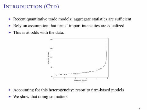
I Recent quantitative trade models: aggregate statistics are sufficientI Rely on assumption that firms’ import intensities are equalizedI This is at odds with the data:
0
.02
.04
.06
.08
Fra
ctio
n of
firm
s
0 .2 .4 .6 .8 1Domestic shares
I Accounting for this heterogeneity: resort to firm-based modelsI We show that doing so matters
2
OUR APPROACH (I): MICRO SUFFICIENCY
0
.02
.04
.06
.08
Fra
ctio
n of
firm
s
0 .2 .4 .6 .8 1Domestic shares
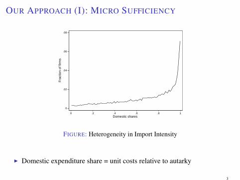
FIGURE: Heterogeneity in Import Intensity
I Domestic expenditure share = unit costs relative to autarky
3

OUR APPROACH (II): MACRO SUFFICIENCY
0
.02
.04
.06
.08
Fra
ctio
n of
firm
s
-10 -5 0 5 10log value added
Importers Non importers
.4.6
.81
Dom
estic
sha
re
1 2 3 4 5 6 7 8 9 10 11 12 13 14 15 16 17 18 19 20Quantiles of value added
25th to 75th percentiles Mean
FIGURE: Import Intensity and Firm Size in France
I Data on value added and domestic shares is sufficient for change inconsumer prices
I Holds in class of models where demand is CESI Arbitrary extensive margin of trade
4
RELATED LITERATURE
I Trade and Consumer Prices:I Feenstra (1994), Broda and Weinstein (2006), Arkolakis, Costinot and
Rodriguez-Clare (2012)
I Aggregate models with input trade:I Eaton, Kortum and Kramarz (2011), Caliendo and Parro (2014), Costinot
and Rodriguez-Clare (2014)
I Models of importing with firm heterogeneity:I Halpern, Koren and Szeidl (2015), Gopinath and Neiman (2014),
Ramanarayanan (2015)I Antras, Fort and Tintelnot (2014), Lu, Asier and Mejia (2015)
I Reduced-form analysis of trade reforms:I Amiti and Konings (2007), Goldberg, Khandelwal, Pavcnik and Topalova
(2010), Amiti, Dai, Feenstra and Romalis (2016),
5
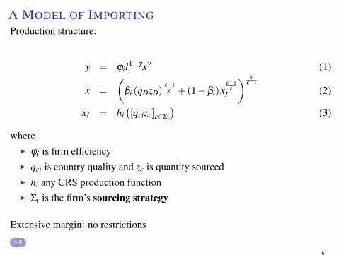
A MODEL OF IMPORTINGProduction structure:
y = ϕil1−γxγ (1)
x =
(βi (qDzD)
ε−1ε +(1−βi)x
ε−1ε
I
) ε
ε−1
(2)
xI = hi([qcizc]c∈Σi
)(3)
whereI ϕi is firm efficiencyI qci is country quality and zc is quantity sourcedI hi any CRS production functionI Σi is the firm’s sourcing strategy
Extensive margin: no restrictions
MP
6
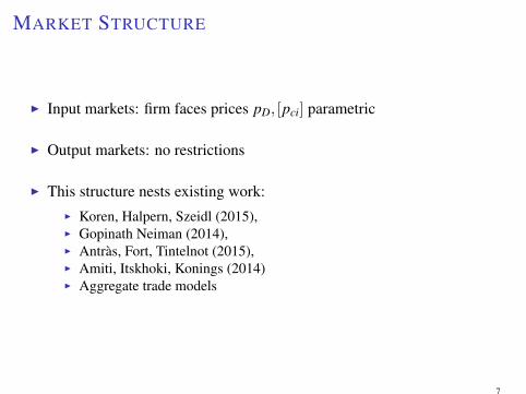
MARKET STRUCTURE
I Input markets: firm faces prices pD, [pci] parametric
I Output markets: no restrictions
I This structure nests existing work:I Koren, Halpern, Szeidl (2015),I Gopinath Neiman (2014),I Antràs, Fort, Tintelnot (2015),I Amiti, Itskhoki, Konings (2014)I Aggregate trade models
7

IMPORT DEMAND
Unit cost is given by
ui =1ϕi
w1−γQi (Σi)γ
where
Qi (Σi) =(
βεi (pD/qD)
1−ε +(1−βi)ε Ai (Σi)
1−ε) 1
1−ε
and Ai (Σi) is the price index of the foreign bundle
8
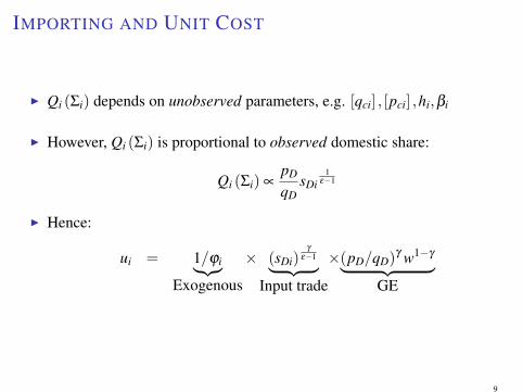
IMPORTING AND UNIT COST
I Qi (Σi) depends on unobserved parameters, e.g. [qci] , [pci] ,hi,βi
I However, Qi (Σi) is proportional to observed domestic share:
Qi (Σi) ∝pD
qDsDi
1ε−1
I Hence:
ui = 1/ϕi︸︷︷︸Exogenous
× (sDi)γ
ε−1︸ ︷︷ ︸Input trade
×(pD/qD)γ w1−γ︸ ︷︷ ︸
GE
9
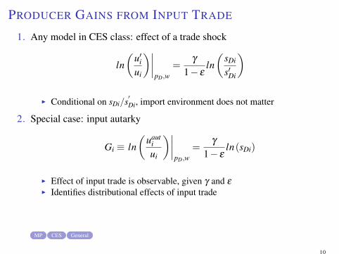
PRODUCER GAINS FROM INPUT TRADE
1. Any model in CES class: effect of a trade shock
ln(
u′iui
)∣∣∣∣pD,w
=γ
1− εln(
sDi
s′Di
)
I Conditional on sDi/s′Di, import environment does not matter
2. Special case: input autarky
Gi ≡ ln(
uautiui
)∣∣∣∣pD,w
=γ
1− εln(sDi)
I Effect of input trade is observable, given γ and ε
I Identifies distributional effects of input trade
MP CES General
10

FROM MICRO TO MACRO
I So far: distribution of unit cost changes across firms
I Now: quantify effect of input trade on consumer prices
I Need to take a stand on:
1. Consumer demand and output market structure
2. Linkages across producers
11

THE MACRO MODEL
I Multi-sector CES monopolistic competition structureI Consumers:
U =S
∏s=1
Cαss (4)
Cs =
(∫ Ns
0c
σs−1σs
is di) σs
σs−1
(5)
I Firm i in sector s:
yi = ϕil1−γsxγs
x =
(βi (qDszDs)
εs−1εs +(1−βi)x
εs−1εs
I
) εsεs−1
I Domestic bundle:
zDs =S
∏j=1
Yζ s
jj
where Yj is akin to (5)12

INPUT TRADE AND CONSUMER PRICES
PROPOSITIONLet P be the consumer price index. For any trade shock,
ln(
P′/P)= α
′(
Γ(I−Ξ×Γ)−1Ξ+ I
)×Λ
where Ξ≡ ζ sj , Γ = diag(γ) , and
Λs =1
1−σsln
(∫ Ns
0
vai∫vaidi
(sDi
s′Di
) γsεs−1 (σs−1)
di
).
I Change in consumer prices fully determined from[vai,
sDis′Di
]i
I Special case of autarky:
ΛAuts =
11−σs
ln(∫ Ns
0
vai∫vaidi
sγs
εs−1 (σs−1)Di di
).
Single Sector Proof Markups
13

METHODOLOGY
I Structural approach to evaluate trade shocks (e.g. Halpern, Koren andSzeidl (2015)):
I Specify extensive margin, e.g. fixed costs FC Model
I Specify import environment [pci,qci, fci,hi,βi]
I Estimate model: deal with computational complexityI Evaluate Qi (Σi)
I We measure unit cost changes by relying on domestic shares:
I Robustness: do not need to specify the import environment.
I Flexibility: easily incorporate multiple sectors with rich I/O structure,general equilibrium and strategic pricing.
I Limitation: requires domestic shares (past policies).
14
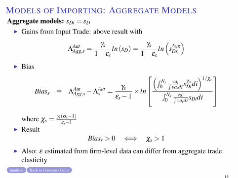
MODELS OF IMPORTING: AGGREGATE MODELSAggregate models: sDi = sD
I Gains from Input Trade: above result with
ΛAutAgg,s =
γs
1− εsln(sD) =
γs
1− εsln(
sAggDs
)I Bias
Biass ≡ ΛAutAgg,s−Λ
Auts =
γs
εs−1× ln
(∫ Ns
0vai∫vaidi s
χsDidi
)1/χs
∫ Ns0
vai∫vaidi sDidi
where χs =
γs(σs−1)εs−1
I ResultBiass > 0 ⇐⇒ χs > 1
I Also: ε estimated from firm-level data can differ from aggregate tradeelasticity
Intuition Back to Consumer Gains
15
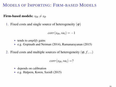
MODELS OF IMPORTING: FIRM-BASED MODELS
Firm-based models: sDi 6= sD
1. Fixed costs and single source of heterogeneity (ϕ)
corr (sDi,vai) =−1
I tends to amplify gainsI e.g. Gopinath and Neiman (2014), Ramanarayanan (2015)
2. Fixed costs and multiple sources of heterogeneity (ϕ, f , ...)
corr (sDi,vai) =?
I depends on calibrationI e.g. Halpern, Koren, Szeidl (2015)
16

QUANTIFYING THE GAINS
I Gains from Input Trade: Consumer prices relative to autarky
I Application to French micro dataI Population of manufacturing firmsI Customs data matched to fiscal data at firm-level
I Need to estimate parameters:
I Estimate (Ξ,α) from aggregate dataI Can be read off Input-Output matrix
I Estimate (ε,γ,σ) from micro dataI σ : from profit margins, σs ∈ [1.8,6]I (ε,γ): see below
Standard Parameters
17
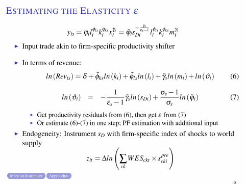
ESTIMATING THE ELASTICITY ε
yis = ϕilφlsi kφks
i xγsi = ϕ̃is
− γsεs−1
Di lφlsi kφks
i mγsi
I Input trade akin to firm-specific productivity shifter
I In terms of revenue:
ln(Revis) = δ + φ̃ksln(ki)+ φ̃lsln(li)+ γ̃sln(mi)+ ln(ϑi) (6)
ln(ϑi) = − 1εs−1
γ̃sln(sDi)+σs−1
σsln(ϕ̃i) (7)
I Get productivity residuals from (6), then get ε from (7)I Or estimate (6)-(7) in one step; PF estimation with additional input
I Endogeneity: Instrument sD with firm-specific index of shocks to worldsupply
zit = ∆ln
(∑ck
WESckt × sprecki
)More on Instrument Approaches
18
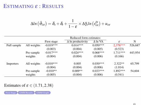
ESTIMATING ε : RESULTS
∆ln(ϑ̂ist)= δs +δt +
11− ε
×∆γ̃sln(sD
ist)+uist
Reduced form estimates:First stage ∆ ln productivity ∆ ln VA ε N
Full sample All weights -0.019*** 0.014*** 0.050*** 2.378*** 526,687(0.003) (0.004) (0.005) (0.523)
Pre-sample -0.017*** 0.024*** 0.068*** 1.711*** 443,954weights (0.004) (0.004) (0.006) (0.166)
Importers All weights -0.010*** 0.005 0.030*** 2.322** 65,799(0.004) (0.004) (0.006) (1.014)
Pre-sample -0.010** 0.009** 0.033*** 1.892*** 54,604weights (0.005) (0.004) (0.006) (0.541)
Estimates of ε ∈ (1.71,2.38)
First Stage GMM Results GMM Graph
19
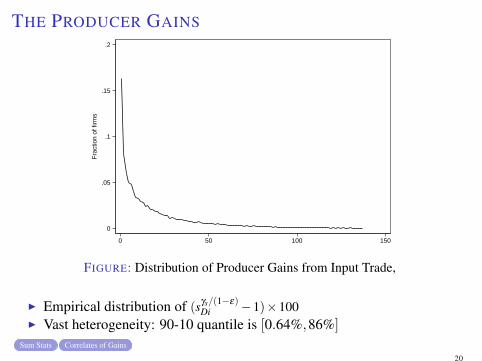
THE PRODUCER GAINS
0
.05
.1
.15
.2
Fra
ctio
n of
firm
s
0 50 100 150
FIGURE: Distribution of Producer Gains from Input Trade,
I Empirical distribution of (sγs/(1−ε)Di −1)×100
I Vast heterogeneity: 90-10 quantile is [0.64%,86%]
Sum Stats Correlates of Gains
20
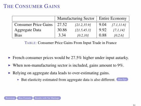
THE CONSUMER GAINS
Manufacturing Sector Entire EconomyConsumer Price Gains 27.52 [21.2,35.9] 9.04 [7.1,11.6]
Aggregate Data 30.86 [21.5,45.3] 9.92 [7.1,14]
Bias 3.34 [0.2,10] 0.88 [0,2.6]
TABLE: Consumer Price Gains From Input Trade in France
I French consumer prices would be 27.5% higher under input autarky.
I When non-manufacturing sector is included, gains amount to 9%.
I Relying on aggregate data leads to over-estimating gains.I But elasticity estimated from aggregate data is also different. Bias Eps
Bootstrap Bias Formula Results with Var Markups
21
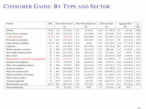
CONSUMER GAINS: BY TYPE AND SECTOR
Industry ISIC Sectoral Price Gains Direct Price Reductions Domestic Inputs Aggregate Data χs
(1) (2) (3) (4) (5)Mining 10-14 7.8 [5.2,10.3] 3.0 [1.8,4.2] 14.9 [11.1,19.2] 2.5 [1.6,3.6] 0.38
Food, tobacco, beverages 15-16 17.8 [12.4,23.4] 11.1 [7.5,14.6] 8.4 [6.2,10.6] 12.6 [7.8,18.2] 1.50
Textiles and leather 17-19 55.6 [42.4,74] 31.1 [24.2,39.9] 31.4 [24.3,40.3] 31.9 [22.4,46.9] 1.07
Wood and wood products 20 14.4 [11.1,18.2] 8.2 [6.4,10.5] 9.6 [7.4,12.1] 9.6 [6.7,13.7] 1.59
Paper, printing, publishing 21-22 20.1 [14.7,26.5] 12.2 [9,16] 14.5 [10.9,18.7] 11.0 [7.7,15.4] 0.64
Chemicals 24 45.1 [32.7,60.7] 27.2 [20.1,36.4] 21.6 [16.1,28.2] 28.1 [18.7,41.8] 1.11
Rubber and plastics products 25 38.4 [27.5,50.9] 20.1 [14.3,26.5] 27.3 [20.2,36] 21.5 [13.9,31] 1.30
Non-metallic mineral products 26 20.8 [15.3,27.4] 13.4 [9.6,17.9] 12.7 [9.7,16.3] 13.3 [9,19] 0.95
Basic metals 27 38.9 [28.2,50.2] 21.8 [16.3,27.7] 21.5 [16.4,27.3] 28.8 [19,41.6] 2.42
Metal products (ex machinery and equipment) 28 18.3 [13.8,23.5] 8.2 [6.2,10.5] 20.5 [15.5,26.2] 7.7 [5.5,10.8] 0.79
Machinery and equipment 29 31.7 [23,41.6] 17.6 [12.8,23.2] 20.0 [15,25.7] 18.2 [12.2,26.2] 1.13
Office and computing machinery 30 44.6 [31.9,57] 20.4 [15.4,25.5] 25.2 [18.3,32.1] 37.0 [22.4,60.3] 3.76
Electrical machinery 31 36.1 [26.4,46.6] 19.8 [14.6,25.6] 23.9 [17.7,30.6] 21.6 [14.8,30.7] 1.51
Radio and communication 32 38.5 [23.5,54.8] 21.5 [13.1,31.1] 23.3 [16.6,30.5] 22.1 [12.5,36.1] 1.11
Medical and optical instruments 33 29.2 [21.1,38.3] 17.9 [12.8,23.4] 20.4 [15.1,26.2] 15.9 [10.7,22.5] 0.70
Motor vehicles, trailers 34 23.3 [17.4,39] 6.2 [3.2,16.4] 21.7 [17,29.3] 11.2 [6.1,24.3] 3.22
Transport equipment 35 22.9 [16,33.2] 15.3 [10.5,22] 19.9 [14.5,27.2] 11.8 [7.9,18.2] 0.22
Manufacturing, recycling 36-37 26.0 [19.2,33.4] 12.9 [9.7,16.3] 19.0 [14.5,24] 14.1 [9.5,20.4] 1.35
Non-manufacturing 3.0 [2.3,3.8] 0.0 [0,0] 7.5 [5.7,9.4] 0.0 [0,0]
22
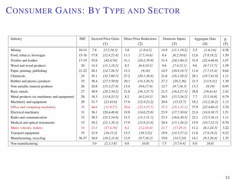
CONSUMER GAINS: BY TYPE AND SECTOR
Industry ISIC Sectoral Price Gains Direct Price Reductions Domestic Inputs Aggregate Data χs
(1) (2) (3) (4) (5)Mining 10-14 7.8 [5.2,10.3] 3.0 [1.8,4.2] 14.9 [11.1,19.2] 2.5 [1.6,3.6] 0.38
Food, tobacco, beverages 15-16 17.8 [12.4,23.4] 11.1 [7.5,14.6] 8.4 [6.2,10.6] 12.6 [7.8,18.2] 1.50
Textiles and leather 17-19 55.6 [42.4,74] 31.1 [24.2,39.9] 31.4 [24.3,40.3] 31.9 [22.4,46.9] 1.07
Wood and wood products 20 14.4 [11.1,18.2] 8.2 [6.4,10.5] 9.6 [7.4,12.1] 9.6 [6.7,13.7] 1.59
Paper, printing, publishing 21-22 20.1 [14.7,26.5] 12.2 [9,16] 14.5 [10.9,18.7] 11.0 [7.7,15.4] 0.64
Chemicals 24 45.1 [32.7,60.7] 27.2 [20.1,36.4] 21.6 [16.1,28.2] 28.1 [18.7,41.8] 1.11
Rubber and plastics products 25 38.4 [27.5,50.9] 20.1 [14.3,26.5] 27.3 [20.2,36] 21.5 [13.9,31] 1.30
Non-metallic mineral products 26 20.8 [15.3,27.4] 13.4 [9.6,17.9] 12.7 [9.7,16.3] 13.3 [9,19] 0.95
Basic metals 27 38.9 [28.2,50.2] 21.8 [16.3,27.7] 21.5 [16.4,27.3] 28.8 [19,41.6] 2.42
Metal products (ex machinery and equipment) 28 18.3 [13.8,23.5] 8.2 [6.2,10.5] 20.5 [15.5,26.2] 7.7 [5.5,10.8] 0.79
Machinery and equipment 29 31.7 [23,41.6] 17.6 [12.8,23.2] 20.0 [15,25.7] 18.2 [12.2,26.2] 1.13
Office and computing machinery 30 44.6 [31.9,57] 20.4 [15.4,25.5] 25.2 [18.3,32.1] 37.0 [22.4,60.3] 3.76
Electrical machinery 31 36.1 [26.4,46.6] 19.8 [14.6,25.6] 23.9 [17.7,30.6] 21.6 [14.8,30.7] 1.51
Radio and communication 32 38.5 [23.5,54.8] 21.5 [13.1,31.1] 23.3 [16.6,30.5] 22.1 [12.5,36.1] 1.11
Medical and optical instruments 33 29.2 [21.1,38.3] 17.9 [12.8,23.4] 20.4 [15.1,26.2] 15.9 [10.7,22.5] 0.70
Motor vehicles, trailers 34 23.3 [17.4,39] 6.2 [3.2,16.4] 21.7 [17,29.3] 11.2 [6.1,24.3] 3.22
Transport equipment 35 22.9 [16,33.2] 15.3 [10.5,22] 19.9 [14.5,27.2] 11.8 [7.9,18.2] 0.22
Manufacturing, recycling 36-37 26.0 [19.2,33.4] 12.9 [9.7,16.3] 19.0 [14.5,24] 14.1 [9.5,20.4] 1.35
Non-manufacturing 3.0 [2.3,3.8] 0.0 [0,0] 7.5 [5.7,9.4] 0.0 [0,0]
23
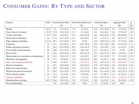
CONSUMER GAINS: BY TYPE AND SECTOR
Industry ISIC Sectoral Price Gains Direct Price Reductions Domestic Inputs Aggregate Data χs
(1) (2) (3) (4) (5)Mining 10-14 7.8 [5.2,10.3] 3.0 [1.8,4.2] 14.9 [11.1,19.2] 2.5 [1.6,3.6] 0.38
Food, tobacco, beverages 15-16 17.8 [12.4,23.4] 11.1 [7.5,14.6] 8.4 [6.2,10.6] 12.6 [7.8,18.2] 1.50
Textiles and leather 17-19 55.6 [42.4,74] 31.1 [24.2,39.9] 31.4 [24.3,40.3] 31.9 [22.4,46.9] 1.07
Wood and wood products 20 14.4 [11.1,18.2] 8.2 [6.4,10.5] 9.6 [7.4,12.1] 9.6 [6.7,13.7] 1.59
Paper, printing, publishing 21-22 20.1 [14.7,26.5] 12.2 [9,16] 14.5 [10.9,18.7] 11.0 [7.7,15.4] 0.64
Chemicals 24 45.1 [32.7,60.7] 27.2 [20.1,36.4] 21.6 [16.1,28.2] 28.1 [18.7,41.8] 1.11
Rubber and plastics products 25 38.4 [27.5,50.9] 20.1 [14.3,26.5] 27.3 [20.2,36] 21.5 [13.9,31] 1.30
Non-metallic mineral products 26 20.8 [15.3,27.4] 13.4 [9.6,17.9] 12.7 [9.7,16.3] 13.3 [9,19] 0.95
Basic metals 27 38.9 [28.2,50.2] 21.8 [16.3,27.7] 21.5 [16.4,27.3] 28.8 [19,41.6] 2.42
Metal products (ex machinery and equipment) 28 18.3 [13.8,23.5] 8.2 [6.2,10.5] 20.5 [15.5,26.2] 7.7 [5.5,10.8] 0.79
Machinery and equipment 29 31.7 [23,41.6] 17.6 [12.8,23.2] 20.0 [15,25.7] 18.2 [12.2,26.2] 1.13
Office and computing machinery 30 44.6 [31.9,57] 20.4 [15.4,25.5] 25.2 [18.3,32.1] 37.0 [22.4,60.3] 3.76
Electrical machinery 31 36.1 [26.4,46.6] 19.8 [14.6,25.6] 23.9 [17.7,30.6] 21.6 [14.8,30.7] 1.51
Radio and communication 32 38.5 [23.5,54.8] 21.5 [13.1,31.1] 23.3 [16.6,30.5] 22.1 [12.5,36.1] 1.11
Medical and optical instruments 33 29.2 [21.1,38.3] 17.9 [12.8,23.4] 20.4 [15.1,26.2] 15.9 [10.7,22.5] 0.70
Motor vehicles, trailers 34 23.3 [17.4,39] 6.2 [3.2,16.4] 21.7 [17,29.3] 11.2 [6.1,24.3] 3.22
Transport equipment 35 22.9 [16,33.2] 15.3 [10.5,22] 19.9 [14.5,27.2] 11.8 [7.9,18.2] 0.22
Manufacturing, recycling 36-37 26.0 [19.2,33.4] 12.9 [9.7,16.3] 19.0 [14.5,24] 14.1 [9.5,20.4] 1.35
Non-manufacturing 3.0 [2.3,3.8] 0.0 [0,0] 7.5 [5.7,9.4] 0.0 [0,0]
24

BEYOND AUTARKY AND CONSUMER PRICES
I So far, change in consumer prices relative to autarkyI using observed distribution of (sD,va)
I Now:I Currency devaluation: (finite) increase in the price of foreign varietiesI Welfare: take into account resources lost through extensive margin
WW aut =
Paut
P×
(L−
∫ Ni lΣidiL
)
I Need a theory of domestic shares:I Take a stand on extensive margin: fixed costs Details
I Impose functional form assumptions on [pc,qc, fc], form for hiI Balanced trade Closing
I One-sector model
I Calibrate the model25
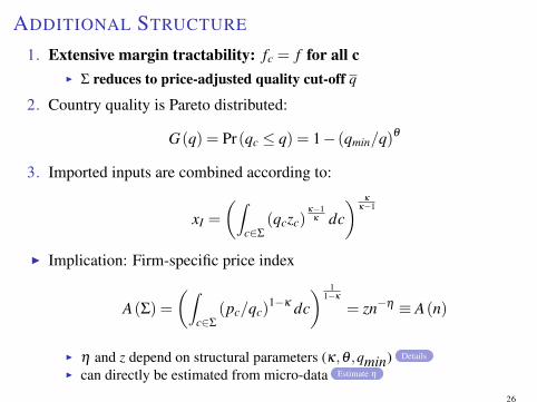
ADDITIONAL STRUCTURE
1. Extensive margin tractability: fc = f for all cI Σ reduces to price-adjusted quality cut-off q
2. Country quality is Pareto distributed:
G(q) = Pr(qc ≤ q) = 1− (qmin/q)θ
3. Imported inputs are combined according to:
xI =
(∫c∈Σ
(qczc)κ−1
κ dc) κ
κ−1
I Implication: Firm-specific price index
A(Σ) =
(∫c∈Σ
(pc/qc)1−κ dc
) 11−κ
= zn−η ≡ A(n)
I η and z depend on structural parameters (κ,θ ,qmin) Details
I can directly be estimated from micro-data Estimate η
26
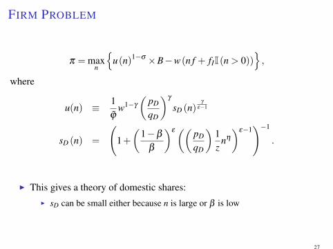
FIRM PROBLEM
π = maxn
{u(n)1−σ ×B−w(n f + fII(n > 0))
},
where
u(n) ≡ 1ϕ̃
w1−γ
(pD
qD
)γ
sD (n)γ
ε−1
sD (n) =
(1+(
1−β
β
)ε(( pD
qD
)1z
nη
)ε−1)−1
.
I This gives a theory of domestic shares:I sD can be small either because n is large or β is low
27
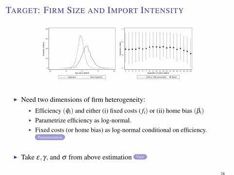
TARGET: FIRM SIZE AND IMPORT INTENSITY
0
.02
.04
.06
.08
Fra
ctio
n of
firm
s
-10 -5 0 5 10log value added
Importers Non importers
.4.6
.81
Dom
estic
sha
re
1 2 3 4 5 6 7 8 9 10 11 12 13 14 15 16 17 18 19 20Quantiles of value added
25th to 75th percentiles Mean
I Need two dimensions of firm heterogeneity:I Efficiency (ϕ̃i) and either (i) fixed costs ( fi) or (ii) home bias (βi)
I Parametrize efficiency as log-normal.I Fixed costs (or home bias) as log-normal conditional on efficiency.
Parametrization
I Take ε,γ, and σ from above estimation View
28
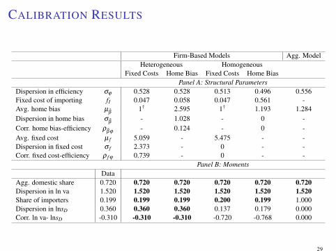
CALIBRATION RESULTS
Firm-Based Models Agg. ModelHeterogeneous Homogeneous
Fixed Costs Home Bias Fixed Costs Home BiasPanel A: Structural Parameters
Dispersion in efficiency σϕ 0.528 0.528 0.513 0.496 0.556Fixed cost of importing fI 0.047 0.058 0.047 0.561 -Avg. home bias µ
β̃1† 2.595 1† 1.193 1.284
Dispersion in home bias σβ̃
- 1.028 - 0 -Corr. home bias-efficiency ρ
β̃ϕ- 0.124 - 0 -
Avg. fixed cost µ f 5.059 - 5.475 - -Dispersion in fixed cost σ f 2.373 - 0 - -Corr. fixed cost-efficiency ρ f ϕ 0.739 - 0 - -
Panel B: MomentsData
Agg. domestic share 0.720 0.720 0.720 0.720 0.720 0.720Dispersion in ln va 1.520 1.520 1.520 1.520 1.520 1.520Share of importers 0.199 0.199 0.199 0.200 0.199 1.000Dispersion in lnsD 0.360 0.360 0.360 0.137 0.179 0.000Corr. ln va- lnsD -0.310 -0.310 -0.310 -0.720 -0.768 0.000
29
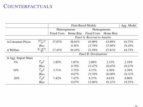
COUNTERFACTUALS
Firm-Based Models Agg. ModelHeterogeneous Homogeneous
Fixed Costs Home Bias Fixed Costs Home BiasPanel A: Reversal to Autarky
∆ Consumer Prices PAut−PP 37.87% 38.01% 43.09% 43.89% 44.73%
Bias 0.36% 13.78% 15.90% 18.10%∆ Welfare W−W Aut
W 17.43% 36.42% 21.59% 27.81% 44.73%Panel B: Devaluations
∆ Agg. Import Share5% P′−P
P 1.85% 1.87% 2.08% 2.15% 2.19%Bias 0.79% 12.47% 16.05% 18.21%
10% P′−PP 3.71% 3.73% 4.17% 4.30% 4.39%
Bias 0.67% 12.58% 16.08% 18.31%20% P′−P
P 7.42% 7.47% 8.37% 8.63% 8.80%Bias 0.67% 12.86% 16.31% 18.55%
30
COUNTERFACTUALS: RESULT #1
Firm-Based Models Agg. ModelHeterogeneous Homogeneous
Fixed Costs Home Bias Fixed Costs Home BiasPanel A: Reversal to Autarky
∆ Consumer Prices PAut−PP 37.87% 38.01% 43.09% 43.89% 44.73%
Bias 0.36% 13.78% 15.90% 18.10%∆ Welfare W−W Aut
W 17.43% 36.42% 21.59% 27.81% 44.73%Panel B: Devaluations
∆ Agg. Import Share5% P′−P
P 1.85% 1.87% 2.08% 2.15% 2.19%Bias 0.79% 12.47% 16.05% 18.21%
10% P′−PP 3.71% 3.73% 4.17% 4.30% 4.39%
Bias 0.67% 12.58% 16.08% 18.31%20% P′−P
P 7.42% 7.47% 8.37% 8.63% 8.80%Bias 0.67% 12.86% 16.31% 18.55%
31
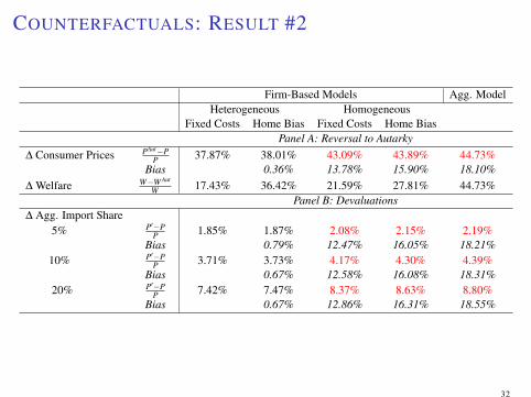
COUNTERFACTUALS: RESULT #2
Firm-Based Models Agg. ModelHeterogeneous Homogeneous
Fixed Costs Home Bias Fixed Costs Home BiasPanel A: Reversal to Autarky
∆ Consumer Prices PAut−PP 37.87% 38.01% 43.09% 43.89% 44.73%
Bias 0.36% 13.78% 15.90% 18.10%∆ Welfare W−W Aut
W 17.43% 36.42% 21.59% 27.81% 44.73%Panel B: Devaluations
∆ Agg. Import Share5% P′−P
P 1.85% 1.87% 2.08% 2.15% 2.19%Bias 0.79% 12.47% 16.05% 18.21%
10% P′−PP 3.71% 3.73% 4.17% 4.30% 4.39%
Bias 0.67% 12.58% 16.08% 18.31%20% P′−P
P 7.42% 7.47% 8.37% 8.63% 8.80%Bias 0.67% 12.86% 16.31% 18.55%
32
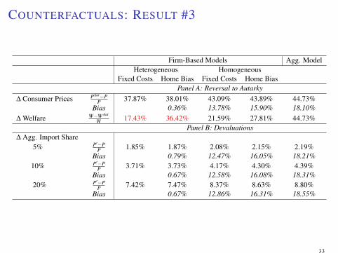
COUNTERFACTUALS: RESULT #3
Firm-Based Models Agg. ModelHeterogeneous Homogeneous
Fixed Costs Home Bias Fixed Costs Home BiasPanel A: Reversal to Autarky
∆ Consumer Prices PAut−PP 37.87% 38.01% 43.09% 43.89% 44.73%
Bias 0.36% 13.78% 15.90% 18.10%∆ Welfare W−W Aut
W 17.43% 36.42% 21.59% 27.81% 44.73%Panel B: Devaluations
∆ Agg. Import Share5% P′−P
P 1.85% 1.87% 2.08% 2.15% 2.19%Bias 0.79% 12.47% 16.05% 18.21%
10% P′−PP 3.71% 3.73% 4.17% 4.30% 4.39%
Bias 0.67% 12.58% 16.08% 18.31%20% P′−P
P 7.42% 7.47% 8.37% 8.63% 8.80%Bias 0.67% 12.86% 16.31% 18.55%
33

COUNTERFACTUALS: SUMMARY
1. Models that match data on size and dom shares predict very similarchanges in consumer prices.
2. Models that do not match data on size and dom shares yieldquantitatively meaningful biases.
I Changes in consumer prices are 14-18% too high.
3. Welfare implications vary substantially across models, even conditionalon matching micro data.
34

CONCLUSIONS
I Input trade is wide-spread but normative implications can be difficult tocharacterize.
I Spending patterns at the firm level are crucial for our understanding ofinput trade:
I Capture unit cost changesI Agnostic about details of import environment
I If micro data on value added is also available, can measure consumerprice gains:
I For reversal to autarky, data is sufficientI For other counterfactuals, data is informativeI Aggregate data gives biased answers
35

Supplementary Material
36

MULTIPLE PRODUCTSBack
I If product aggregator is nested in country aggregator,
qcizc ≡ ψci([qkcizkc]k∈Kci
), (8)
then our analysis goes through unchanged.
I Otherwise, if:
x =
(K
∑k=1
(ηkxk)ι−1
ι
) ι
ι−1
(9)
xk =
(βki (qkDzkD)
εk−1εk +(1−βki)x
εk−1εk
kI
) εkεk−1
(10)
xkI = hki
([qkcizkc]c∈Σki
), (11)
the analysis can be extended but requires domestic shares by product.37
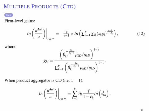
MULTIPLE PRODUCTS (CTD)Back
Firm-level gains:
ln(
uAut
u
)∣∣∣∣pD,w
= γ
ι−1 × ln(
∑Kk=1 χki (skDi)
ι−11−εk
), (12)
where
χki ≡
(β− εk
εk−1
ki pkD/qkD
)1−ι
∑Kk=1
(β− εk
εk−1
ki pkD/qkD
)1−ι.
When product aggregator is CD (i.e. ι = 1):
ln(
uAut
u
)∣∣∣∣pD,w
=K
∑k=1
ηkγ
1− εkln(
skDi
).
38

CES UPPER TIERBack
Suppose that:
y = ϕ
((1− γ) l
ζ−1ζ + γx
ζ−1ζ
) ζ
ζ−1
.
Then:
u =1ϕ
s1
ζ−1M
(1γ
) ζ
ζ−1
s1
ε−1D
(1β
) ε
ε−1(
pD
qD
)∝ s
1ζ−1M s
1ε−1D , (13)
Because sAutM is not observed, we can compute as:
sAutM =
(γ
1−γ
)ζ
β− ε
ε−1 (1−ζ )(
pD/qD
w
)1−ζ
1+(
γ
1−γ
)ζ
β− ε
ε−1 (1−ζ )(
pD/qD
w
)1−ζ. (14)
so that
ln(
uAut
u
)∣∣∣∣pD,w
= ln
1+(
γ
1−γ
)ζ
β− ε
ε−1 (1−ζ )(
pD/qDw
)1−ζ
s1−ζ
ε−1D
1+(
γ
1−γ
)ζ
β− ε
ε−1 (1−ζ )(
pD/qDw
)1−ζ
1ζ−1
(15)
39
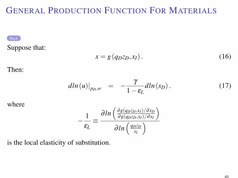
GENERAL PRODUCTION FUNCTION FOR MATERIALS
Back
Suppose that:x = g(qDzD,xI) . (16)
Then:
dln(u)|pD,w = − γ
1− εLdln(sD) . (17)
where
− 1εL≡
∂ ln(
∂g(qDzD,xI)/∂xD∂g(qDzD,xI)/∂xI
)∂ ln(
qDzDxI
)is the local elasticity of substitution.
40
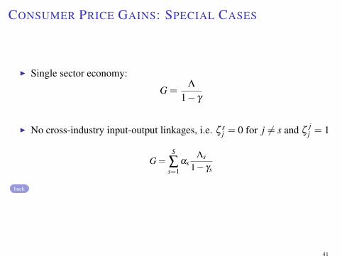
CONSUMER PRICE GAINS: SPECIAL CASES
I Single sector economy:
G =Λ
1− γ
I No cross-industry input-output linkages, i.e. ζ sj = 0 for j 6= s and ζ
jj = 1
G =S
∑s=1
αsΛs
1− γs
back
41

SKETCH OF PROOF
Back
1. Prices are given by
Ps =σs
σs−1
(pDs
qDs
)γs
×
(∫ Ns
0
(1ϕ̃i
sγs/(εs−1)Di
)1−σs
di
) 11−σs
2. Efficiency ϕ̃i is unknown but:
vai = κsϕ̃σs−1i s
γs1−εs
(σs−1)Di
3. Hence
ln(
PAuts
Ps
)= γsln
(pAut
DspDs
)+
11−σs
ln(∫ Ns
0
vai∫vaidi
sγs
εs−1 (σs−1)Di di
)︸ ︷︷ ︸
=ΛAuts
42

VARIABLE MARKUPSBack
I Allow distribution of markups to respond to changes in tradingenvironment.
I As in Edmond, Midrigan and Xu (2012), use setting of Atkeson-Burstein(2008).
I Demand structure:
Cs =
(∫ Ns
0c
σs−1σs
js d j) σs
σs−1
,
c js =
(N js
∑i=1
cθs−1
θsi js
) θsθs−1
,
where θs ≥ σs.
I Firms compete with other firms in their variety j, but take decisions inother sectors as given. Assume Cournot competition.
43
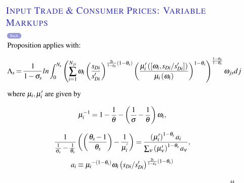
INPUT TRADE & CONSUMER PRICES: VARIABLE
MARKUPSBack
Proposition applies with:
Λs =1
1−σsln∫ Ns
0
(N js
∑i=1
ωi
(sDi
s′Di
) γs1−εs
(1−θs)(µ ′i ([ωi,sDi/s′Di])
µi (ωi)
)1−θs) 1−σs
1−θs
ω jsd j
where µi,µ′i are given by
µ−1i = 1− 1
θ−(
1σ− 1
θ
)ωi,
11σs− 1
θs
((θs−1
θs
)− 1
µ′i
)=
(µ ′i )1−θs ai
∑ν (µ′ν)
1−θs aν
,
ai ≡ µi−(1−θs)ωi
(sDi/s′Di
) γs1−εs
(1−θs)
44
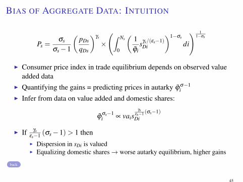
BIAS OF AGGREGATE DATA: INTUITION
Ps =σs
σs−1
(pDs
qDs
)γs
×
(∫ Ns
0
(1ϕ̃i
sγs/(εs−1)Di
)1−σs
di
) 11−σs
I Consumer price index in trade equilibrium depends on observed valueadded data
I Quantifying the gains = predicting prices in autarky ϕ̃σ−1i
I Infer from data on value added and domestic shares:
ϕ̃σs−1i ∝ vais
γsεs−1 (σs−1)Di
I If γsεs−1 (σs−1)> 1 thenI Dispersion in sDi is valuedI Equalizing domestic shares→ worse autarky equilibrium, higher gains
back
45
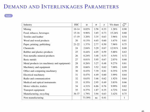
DEMAND AND INTERLINKAGES PARAMETERS
back
Industry ISIC α σ γ VA share sAggD
Mining 10-14 0.02% 2.58 0.33 1.28% 0.90
Food, tobacco, beverages 15-16 9.90% 3.85 0.73 15.24% 0.80
Textiles and leather 17-19 3.20% 3.35 0.63 3.96% 0.54
Wood and wood products 20 0.13% 4.65 0.60 1.67% 0.81
Paper, printing, publishing 21-22 1.37% 2.77 0.50 7.96% 0.75
Chemicals 24 2.04% 3.29 0.67 12.91% 0.60
Rubber and plastics products 25 0.44% 4.05 0.59 5.88% 0.63
Non-metallic mineral products 26 0.24% 3.48 0.53 4.54% 0.72
Basic metals 27 0.01% 5.95 0.67 2.07% 0.60
Metal products (ex machinery and equipment) 28 0.26% 3.27 0.48 9.27% 0.81
Machinery and equipment 29 0.66% 3.52 0.62 7.00% 0.69
Office and computing machinery 30 0.43% 7.39 0.81 0.35% 0.59
Electrical machinery 31 0.47% 4.49 0.60 3.99% 0.64
Radio and communication 32 0.63% 3.46 0.62 1.92% 0.64
Medical and optical instruments 33 0.35% 2.95 0.49 3.83% 0.66
Motor vehicles, trailers 34 4.31% 6.86 0.76 9.99% 0.82
Transport equipment 35 0.37% 1.87 0.35 4.72% 0.64
Manufacturing, recycling 36-37 1.79% 3.94 0.63 3.42% 0.75
Non-manufacturing 73.39% na 0.41 1
46
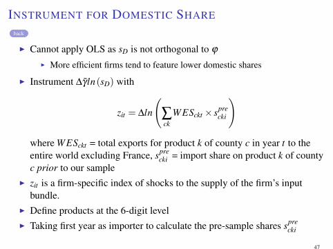
INSTRUMENT FOR DOMESTIC SHARE
back
I Cannot apply OLS as sD is not orthogonal to ϕ
I More efficient firms tend to feature lower domestic shares
I Instrument ∆γ̃ln(sD) with
zit = ∆ln
(∑ck
WESckt × sprecki
)
where WESckt = total exports for product k of county c in year t to theentire world excluding France, spre
cki = import share on product k of countyc prior to our sample
I zit is a firm-specific index of shocks to the supply of the firm’s inputbundle.
I Define products at the 6-digit levelI Taking first year as importer to calculate the pre-sample shares spre
cki
47
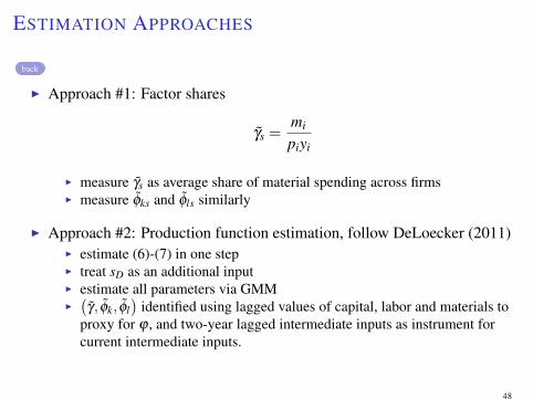
ESTIMATION APPROACHES
back
I Approach #1: Factor shares
γ̃s =mi
piyi
I measure γ̃s as average share of material spending across firmsI measure φ̃ks and φ̃ls similarly
I Approach #2: Production function estimation, follow DeLoecker (2011)I estimate (6)-(7) in one stepI treat sD as an additional inputI estimate all parameters via GMMI(γ̃, φ̃k, φ̃l
)identified using lagged values of capital, labor and materials to
proxy for ϕ , and two-year lagged intermediate inputs as instrument forcurrent intermediate inputs.
48
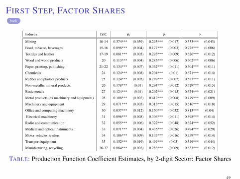
FIRST STEP, FACTOR SHARESback
Industry ISIC φk φl γ
Mining 10-14 0.374*** (0.039) 0.293*** (0.017) 0.333*** (0.043)
Food, tobacco, beverages 15-16 0.098*** (0.004) 0.177*** (0.003) 0.725*** (0.006)
Textiles and leather 17-19 0.081*** (0.003) 0.293*** (0.009) 0.626*** (0.012)
Wood and wood products 20 0.113*** (0.004) 0.285*** (0.006) 0.602*** (0.006)
Paper, printing, publishing 21-22 0.134*** (0.007) 0.362*** (0.011) 0.504*** (0.011)
Chemicals 24 0.124*** (0.008) 0.204*** (0.01) 0.671*** (0.014)
Rubber and plastics products 25 0.124*** (0.005) 0.289*** (0.007) 0.587*** (0.011)
Non-metallic mineral products 26 0.178*** (0.01) 0.294*** (0.012) 0.529*** (0.015)
Basic metals 27 0.124*** (0.01) 0.202*** (0.015) 0.674*** (0.021)
Metal products (ex machinery and equipment) 28 0.108*** (0.002) 0.412*** (0.008) 0.479*** (0.009)
Machinery and equipment 29 0.071*** (0.003) 0.313*** (0.015) 0.616*** (0.018)
Office and computing machinery 30 0.037*** (0.012) 0.150*** (0.032) 0.813*** (0.04)
Electrical machinery 31 0.096*** (0.008) 0.306*** (0.011) 0.598*** (0.014)
Radio and communication 32 0.055*** (0.006) 0.322*** (0.048) 0.624*** (0.052)
Medical and optical instruments 33 0.071*** (0.004) 0.435*** (0.026) 0.494*** (0.029)
Motor vehicles, trailers 34 0.106*** (0.009) 0.135*** (0.016) 0.759*** (0.014)
Transport equipment 35 0.152*** (0.019) 0.499*** (0.03) 0.349*** (0.044)
Manufacturing, recycling 36-37 0.084*** (0.003) 0.283*** (0.009) 0.633*** (0.012)
TABLE: Production Function Coefficient Estimates, by 2-digit Sector: Factor Shares
49
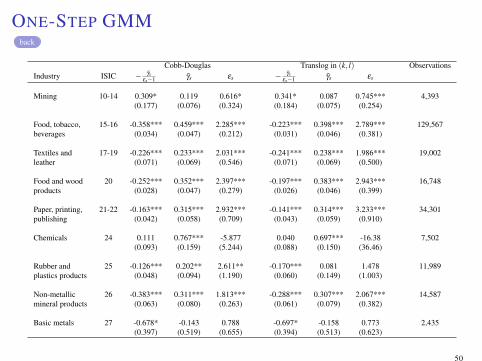
ONE-STEP GMMback
Cobb-Douglas Translog in (k, l) ObservationsIndustry ISIC − γ̃s
εs−1 γ̃s εs − γ̃sεs−1 γ̃s εs
Mining 10-14 0.309* 0.119 0.616* 0.341* 0.087 0.745*** 4,393(0.177) (0.076) (0.324) (0.184) (0.075) (0.254)
Food, tobacco, 15-16 -0.358*** 0.459*** 2.285*** -0.223*** 0.398*** 2.789*** 129,567beverages (0.034) (0.047) (0.212) (0.031) (0.046) (0.381)
Textiles and 17-19 -0.226*** 0.233*** 2.031*** -0.241*** 0.238*** 1.986*** 19,002leather (0.071) (0.069) (0.546) (0.071) (0.069) (0.500)
Food and wood 20 -0.252*** 0.352*** 2.397*** -0.197*** 0.383*** 2.943*** 16,748products (0.028) (0.047) (0.279) (0.026) (0.046) (0.399)
Paper, printing, 21-22 -0.163*** 0.315*** 2.932*** -0.141*** 0.314*** 3.233*** 34,301publishing (0.042) (0.058) (0.709) (0.043) (0.059) (0.910)
Chemicals 24 0.111 0.767*** -5.877 0.040 0.697*** -16.38 7,502(0.093) (0.159) (5.244) (0.088) (0.150) (36.46)
Rubber and 25 -0.126*** 0.202** 2.611** -0.170*** 0.081 1.478 11,989plastics products (0.048) (0.094) (1.190) (0.060) (0.149) (1.003)
Non-metallic 26 -0.383*** 0.311*** 1.813*** -0.288*** 0.307*** 2.067*** 14,587mineral products (0.063) (0.080) (0.263) (0.061) (0.079) (0.382)
Basic metals 27 -0.678* -0.143 0.788 -0.697* -0.158 0.773 2,435(0.397) (0.519) (0.655) (0.394) (0.513) (0.623)
50
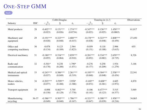
ONE-STEP GMMback
Cobb-Douglas Translog in (k, l) ObservationsIndustry ISIC − γ̃s
εs−1 γ̃s εs − γ̃sεs−1 γ̃s εs
Metal products 28 -0.402*** 0.151*** 1.374*** -0.347*** 0.156*** 1.450*** 61,017(0.023) (0.026) (0.0734) (0.023) (0.025) (0.0865)
Machinery and 29 -0.191*** 0.323*** 2.688*** -0.178*** 0.323*** 2.808*** 27,450equipment (0.028) (0.048) (0.415) (0.028) (0.048) (0.459)
Office and 30 -0.078 0.123 2.564 -0.059 0.118 2.996 655computing machinery (0.134) (0.189) (3.823) (0.131) (0.188) (5.615)
Electrical machinery 31 -0.180*** 0.334*** 2.859*** -0.201*** 0.334*** 2.659*** 8,326(0.055) (0.084) (0.910) (0.052) (0.082) (0.735)
Radio and 32 -0.301* 0.238 1.790* -0.276 0.258 1.934 3,146communication (0.170) (0.208) (1.071) (0.177) (0.209) (1.279)
Medical and optical 33 -0.243*** 0.306*** 2.261*** -0.195*** 0.304*** 2.558*** 22,541instruments (0.037) (0.049) (0.319) (0.040) (0.048) (0.454)
Motor vehicles, 34 -0.203*** 0.599** 3.958* -0.169** 0.608** 4.605 4,870trailers (0.077) (0.288) (2.388) (0.072) (0.281) (2.972)
Transport equipment 35 -0.098 0.462*** 5.705 -0.106 0.477*** 5.515 3,949(0.150) (0.129) (7.770) (0.141) (0.123) (6.577)
Manufacturing, 36-37 -0.386*** 0.303*** 1.786*** -0.321*** 0.308*** 1.958*** 34,863recycling (0.049) (0.040) (0.167) (0.047) (0.039) (0.216)
51
ONE-STEP GMM: RESULTSback
-20
-10
010
20e
Min
ing
Foo
d, to
bacc
o,be
vera
ges
Tex
tiles
and
leat
her
Woo
d pr
oduc
ts
Pap
er, p
rintin
g,pu
blis
hing
Che
mic
als
Rub
ber
and
plas
tics
Non
met
allic
min
eral
pro
duct
s
Bas
ic m
etal
s
Met
al p
rodu
cts
Mac
hine
ry a
ndeq
uipm
ent
Com
putin
gm
achi
nery
Ele
ctric
alm
achi
nery
Rad
io a
ndco
mm
unic
atio
n
Med
ical
inst
rum
ents
Mot
or v
ehic
les
Tra
nspo
rteq
uipm
ent
Rec
yclin
g, n
ec.
Cobb Douglas Translog
52
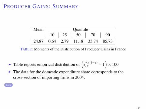
PRODUCER GAINS: SUMMARY
Mean Quantile10 25 50 70 90
24.87 0.64 2.79 11.18 33.74 85.73
TABLE: Moments of the Distribution of Producer Gains in France
I Table reports empirical distribution of(
sγs/(1−ε)Di −1
)×100
I The data for the domestic expenditure share corresponds to thecross-section of importing firms in 2004.
Back
53
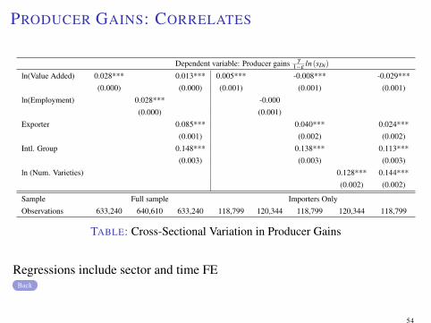
PRODUCER GAINS: CORRELATES
Dependent variable: Producer gains γ
1−εln(sDi)
ln(Value Added) 0.028*** 0.013*** 0.005*** -0.008*** -0.029***
(0.000) (0.000) (0.001) (0.001) (0.001)
ln(Employment) 0.028*** -0.000
(0.000) (0.001)
Exporter 0.085*** 0.040*** 0.024***
(0.001) (0.002) (0.002)
Intl. Group 0.148*** 0.138*** 0.113***
(0.003) (0.003) (0.003)
ln (Num. Varieties) 0.128*** 0.144***
(0.002) (0.002)
Sample Full sample Importers Only
Observations 633,240 640,610 633,240 118,799 120,344 118,799 120,344 118,799
TABLE: Cross-Sectional Variation in Producer Gains
Regressions include sector and time FEBack
54
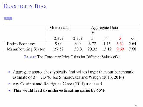
ELASTICITY BIAS
Back
Micro-data Aggregate Dataε
2.378 2.378 3 4 5 6Entire Economy 9.04 9.9 6.72 4.43 3.31 2.64Manufacturing Sector 27.52 30.8 20.32 13.12 9.69 7.68
TABLE: The Consumer Price Gains for Different Values of ε
I Aggregate approaches typically find values larger than our benchmarkestimate of ε = 2.378, see Simonovska and Waugh (2013, 2014)
I e.g. Costinot and Rodriguez-Clare (2014) use ε = 5I This would lead to under-estimating gains by 65%
55
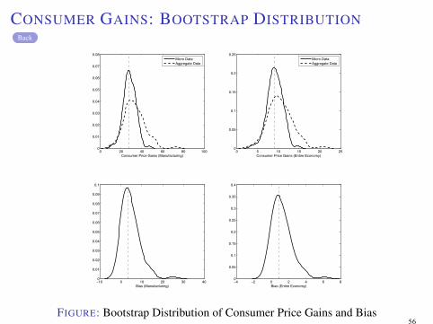
CONSUMER GAINS: BOOTSTRAP DISTRIBUTIONBack
0 5 10 15 20 250
0.05
0.1
0.15
0.2
0.25
Consumer Price Gains (Entire Economy)
Micro DataAggregate Data
0 20 40 60 80 1000
0.01
0.02
0.03
0.04
0.05
0.06
0.07
0.08
Consumer Price Gains (Manufacturing)
Micro DataAggregate Data
−4 −2 0 2 4 6 80
0.05
0.1
0.15
0.2
0.25
0.3
0.35
0.4
Bias (Entire Economy)−10 0 10 20 30 400
0.01
0.02
0.03
0.04
0.05
0.06
0.07
0.08
0.09
0.1
Bias (Manufacturing)
FIGURE: Bootstrap Distribution of Consumer Price Gains and Bias56
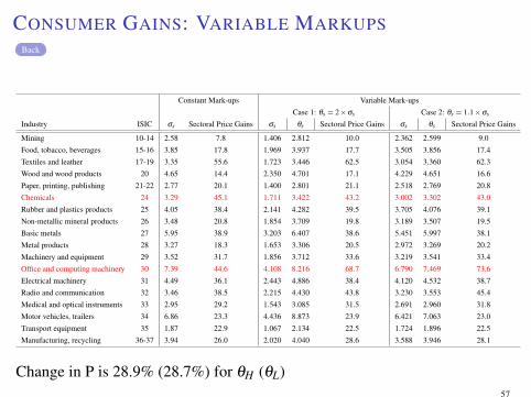
CONSUMER GAINS: VARIABLE MARKUPSBack
Constant Mark-ups Variable Mark-ups
Case 1: θs = 2×σs Case 2: θs = 1.1×σs
Industry ISIC σs Sectoral Price Gains σs θs Sectoral Price Gains σs θs Sectoral Price Gains
Mining 10-14 2.58 7.8 1.406 2.812 10.0 2.362 2.599 9.0
Food, tobacco, beverages 15-16 3.85 17.8 1.969 3.937 17.7 3.505 3.856 17.4
Textiles and leather 17-19 3.35 55.6 1.723 3.446 62.5 3.054 3.360 62.3
Wood and wood products 20 4.65 14.4 2.350 4.701 17.1 4.229 4.651 16.6
Paper, printing, publishing 21-22 2.77 20.1 1.400 2.801 21.1 2.518 2.769 20.8
Chemicals 24 3.29 45.1 1.711 3.422 43.2 3.002 3.302 43.0
Rubber and plastics products 25 4.05 38.4 2.141 4.282 39.5 3.705 4.076 39.1
Non-metallic mineral products 26 3.48 20.8 1.854 3.709 19.8 3.189 3.507 19.5
Basic metals 27 5.95 38.9 3.203 6.407 38.6 5.451 5.997 38.1
Metal products 28 3.27 18.3 1.653 3.306 20.5 2.972 3.269 20.2
Machinery and equipment 29 3.52 31.7 1.856 3.712 33.6 3.219 3.541 33.4
Office and computing machinery 30 7.39 44.6 4.108 8.216 68.7 6.790 7.469 73.6
Electrical machinery 31 4.49 36.1 2.443 4.886 38.4 4.120 4.532 38.7
Radio and communication 32 3.46 38.5 2.215 4.430 43.8 3.230 3.553 45.4
Medical and optical instruments 33 2.95 29.2 1.543 3.085 31.5 2.691 2.960 31.8
Motor vehicles, trailers 34 6.86 23.3 4.436 8.873 23.9 6.421 7.063 23.0
Transport equipment 35 1.87 22.9 1.067 2.134 22.5 1.724 1.896 22.5
Manufacturing, recycling 36-37 3.94 26.0 2.020 4.040 28.6 3.588 3.946 28.1
Change in P is 28.9% (28.7%) for θH (θL)57
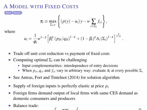
A MODEL WITH FIXED COSTSBack Back2
πi ≡maxΣi,y
{(p(y)−ui)y−w ∑
c∈Σi
fci
},
where
ui =1ϕi
w1−γ
[β
εi (pD/qD)
1−ε +(1−βi)εAi (Σi)
1−ε] γ
1−ε
.
I Trade off unit cost reduction vs payment of fixed costsI Computing optimal Σi can be challenging
I Input complementarities: interdependece of entry decisionsI When pci,qci and fci vary in arbitrary way: evaluate πi at every possible Σi
I See Antras, Fort and Tintelnot (2014) for solution algorithm
I Supply of foreign inputs is perfectly elastic at price pc
I Foreign firms demand output of local firms with same CES demand asdomestic consumers and producers
I Balance trade: ∫ipiyROW
i =∫
i(1− sDi)midi,
where yROWi is foreign demand for firm i’s production.
I Labor market clearing:
L =∫
i
(li + lF
i)
di
Back
58
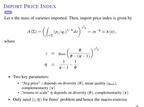
IMPORT PRICE INDEXback
Let n the mass of varieties imported. Then, import price index is given by
A(Σ) =
(∫c∈Σ
(pc/qc)1−κ dc
) 11−κ
= zn−η ≡ A(n) ,
where
z ≡ qmin
(θ
θ − (κ−1)
) 11−κ
η ≡ 1κ−1
− 1θ.
I Two key parameters:I “Avg price” z depends on diversity (θ), mean quality (qmin),
complementarity (κ)I “returns to scale” η depends on diversity (θ), complementarity (κ)
I Only need (z,η) for firms’ problem and hence the macro-exercise59
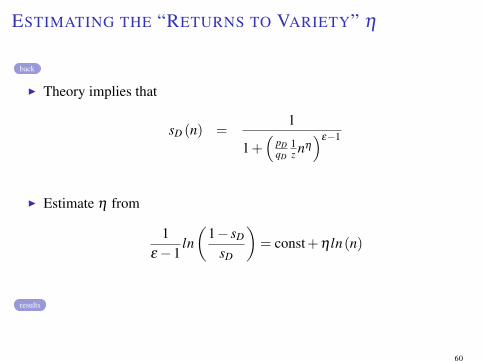
ESTIMATING THE “RETURNS TO VARIETY” η
back
I Theory implies that
sD (n) =1
1+(
pDqD
1z nη
)ε−1
I Estimate η from
1ε−1
ln(
1− sD
sD
)= const+η ln(n)
results
60
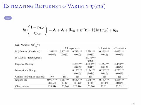
ESTIMATING RETURNS TO VARIETY η(ctd)
back
ln(
1− sDist
sDist
)= δs +δt +δNK +η (ε−1) ln(nist)+uist
Dep. Variable: ln(1−sDsD
)
All Importers > 1 variety > 2 varietiesln (Number of Varieties) 1.308*** 0.707*** 0.733*** 0.739*** 0.526*** 0.463***
(0.009) (0.010) (0.010) (0.010) (0.011) (0.019)ln (Capital / Employment) -0.070***
(0.006)Exporter Dummy -0.395*** -0.388*** -0.254*** -0.198***
(0.013) (0.013) (0.017) (0.029)International Group 0.150*** 0.174*** 0.216*** 0.223***
(0.016) (0.016) (0.016) (0.019)Control for Num of products No Yes Yes Yes Yes YesImplied Eta 0.950*** 0.513*** 0.532*** 0.536*** 0.382*** 0.336***
(0.260) (0.142) (0.147) (0.148) (0.106) (0.096)Observations 120,344 120,344 120,344 120,344 73,651 35,751
61
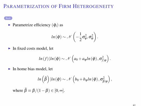
PARAMETRIZATION OF FIRM HETEROGENEITY
Back
I Parametrize efficiency (ϕ̃i) as
ln(ϕ̃)∼N
(−1
2σ
2ϕ ,σ
2ϕ
).
I In fixed costs model, let
ln( f ) |ln(ϕ̃)∼N(
a0 +aϕ ln(ϕ̃) ,σ2f |ϕ
).
I In home bias model, let
ln(
β̃
)|ln(ϕ̃)∼N
(b0 +bϕ ln(ϕ̃) ,σ2
β̃ |ϕ
),
where β̃ ≡ β/(1−β ) ∈ [0,∞].
62
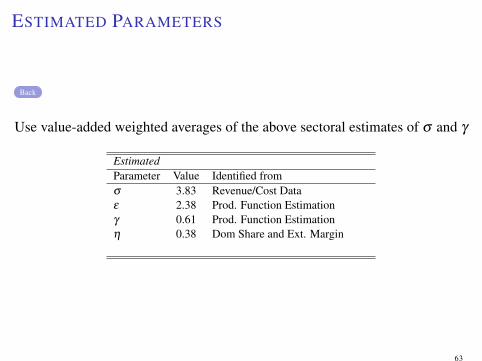
ESTIMATED PARAMETERS
Back
Use value-added weighted averages of the above sectoral estimates of σ and γ
EstimatedParameter Value Identified fromσ 3.83 Revenue/Cost Dataε 2.38 Prod. Function Estimationγ 0.61 Prod. Function Estimationη 0.38 Dom Share and Ext. Margin
63