The g-formula for competing risks - kupublicifsv.sund.ku.dk/~tag/download/ulm-presentation-2017.pdf · The g-formula for competing risks Brice Ozenne & Thomas Alexander Gerds Biostatistics,

The g-formula for competing risks

Brice Ozenne & Thomas Alexander Gerds

Biostatistics, University of Copenhagen

April 21, 2017

1 / 30

Outline

Appetizer

Example 1

Average treatment e�ects

Asymptotics

Software

2 / 30

Appetizer

3 / 30

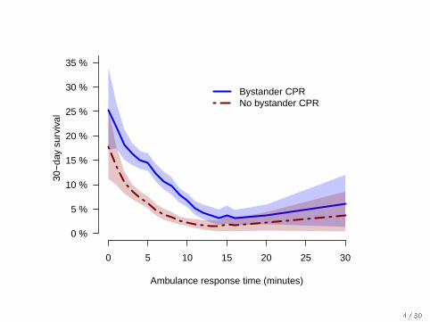
0 5 10 15 20 25 30

0 %

5 %

10 %

15 %

20 %

25 %

30 %

35 %30

−da

y su

rviv

al

Ambulance response time (minutes)

Bystander CPRNo bystander CPR

4 / 30

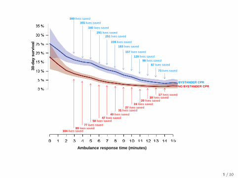
380 lives saved

355 lives saved

340 lives saved

291 lives saved

251 lives saved

228 lives saved

183 lives saved

157 lives saved

120 lives saved

98 lives saved

87 lives saved

NO BYSTANDER CPR

BYSTANDER CPR

89 lives saved 77 lives saved

58 lives saved


18 lives saved



104 lives saved

17 lives saved

73 lives saved

Ambulance response time (minutes)

30

-day s

urv

iva

l

5 / 30

Robin's g-formula and competing risks1

1Robins JM. (1986). A new approach to causal inference in mortalitystudies with sustained exposure periods � Application to control of the healthyworker survivor e�ect. Mathematical Modelling, 7:1393-1512, with 1987 Erratato "A new approach to causal inference in mortality studies with sustainedexposure periods � Application to control of the healthy worker survivor e�ect."Computers and Mathematics with Applications, 14:917-921;

6 / 30

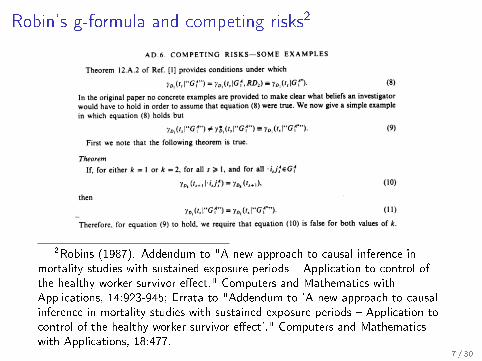
Robin's g-formula and competing risks2

2Robins (1987). Addendum to "A new approach to causal inference inmortality studies with sustained exposure periods � Application to control ofthe healthy worker survivor e�ect." Computers and Mathematics withApplications, 14:923-945; Errata to "Addendum to 'A new approach to causalinference in mortality studies with sustained exposure periods � Application tocontrol of the healthy worker survivor e�ect'." Computers and Mathematicswith Applications, 18:477.

7 / 30

Example 1

8 / 30

9 / 30

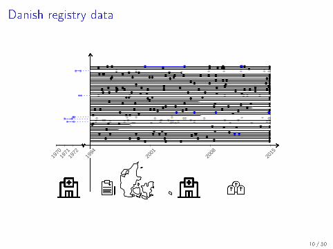
Danish registry data

●

●

●

●

●

●

●

●

●

●

●

●

●

●

●

●

●

●

●

●

●

●

●

●

●

●

1970

1971

1972

1994

2001

2008

2015

● ● ●●

● ● ●● ● ●●

●● ● ● ● ● ● ●●

●● ● ●

●● ●

● ●●● ● ● ●● ● ● ● ● ●

● ● ● ● ●● ● ● ●●● ● ● ● ● ● ●

● ● ●● ● ●● ● ● ● ●

● ● ●● ●

●● ● ●

● ● ● ● ● ● ●● ●

● ● ● ●●

● ● ● ● ●●

●● ●

● ● ● ●● ● ● ● ● ●

● ● ● ●● ● ● ● ●

● ● ●● ● ● ● ● ● ● ● ●

● ● ● ● ● ● ●● ● ●

● ●● ● ●

●● ● ●

● ● ●● ● ● ● ●

● ● ● ● ● ● ●● ●● ●

● ● ● ●● ● ● ● ● ● ●

●● ● ● ● ●●

● ● ● ● ●

●

●

●

●

●

●

● ●

● ● ● ●

● ● ●●

10 / 30

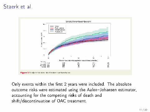
Staerk et al.

Only events within the �rst 2 years were included. The absoluteoutcome risks were estimated using the Aalen�Johansen estimator,accounting for the competing risks of death andshift/discontinuation of OAC treatment.

11 / 30

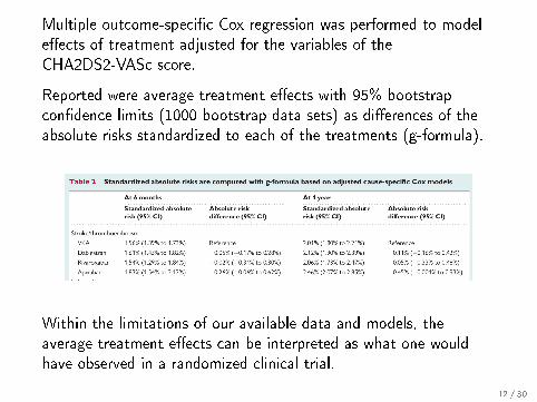
Multiple outcome-speci�c Cox regression was performed to modele�ects of treatment adjusted for the variables of theCHA2DS2-VASc score.

Reported were average treatment e�ects with 95% bootstrapcon�dence limits (1000 bootstrap data sets) as di�erences of theabsolute risks standardized to each of the treatments (g-formula).

Within the limitations of our available data and models, theaverage treatment e�ects can be interpreted as what one wouldhave observed in a randomized clinical trial.

12 / 30

Average treatment e�ects

13 / 30

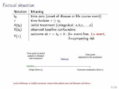
Factual situation

Notation Meaning

t0 time zero (onset of disease or life course event)τ time horizon τ ≥ t0A(t0) initial treatment (categorical: a,b,c,. . . ,o)X(t0) observed baseline confounders

Y(τ)outcome at τ = t0 + h : 0= event-free, 1= event,

2=competing risk

Time point at whichpatient is initiated

with treatment

Time pointattached to the prediction

baseline

followup

Origin (time t0) Outcome evaluation (time τ)

Lost to followup, or (right) censored, means that patient was not followed until time τ.

14 / 30

Parameter of interest

Potential outcomes3:

Yi (τ ; x) = outcome of patient i under initial treatment x

Average treatment e�ect

ATE(τ ; a, b) = P(Y (τ ; a) = 1)− P(Y (τ ; b) = 1)

The ATE is generally understood as a causal parameter (i.e., an

estimate or property of a population) that a researcher desires to

know, de�ned without reference to the study design.

3Rosenbaum and Rubin (1983)15 / 30

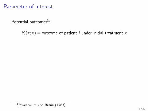
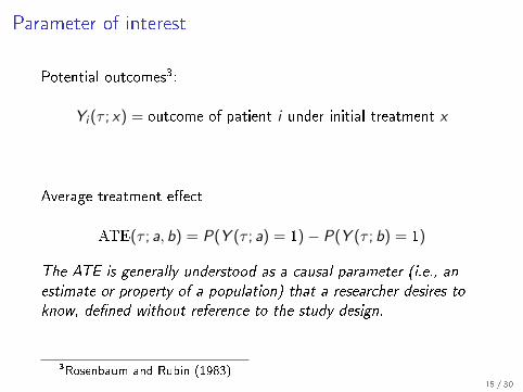
Parameter of interest

Potential outcomes3:

Yi (τ ; x) = outcome of patient i under initial treatment x

Average treatment e�ect

ATE(τ ; a, b) = P(Y (τ ; a) = 1)− P(Y (τ ; b) = 1)

The ATE is generally understood as a causal parameter (i.e., an

estimate or property of a population) that a researcher desires to

know, de�ned without reference to the study design.

3Rosenbaum and Rubin (1983)15 / 30

Substantive model

Observational studies with random treatment assignment mayenable one to estimate ATE in various ways4

An alternative to inverse probability weighting is standardization:

P(Y (τ ; a) = 1) = E[P(Y (τ) = 1|A(t0) = a,X (t0))

]Under exchangeability, consistency etc., g-estimation is often basedon a semiparametric structural nested mean model:

Y ∼ A + X + AX

4Hernan & Robins (book): Ideally, we would estimate the conditional meansnonparametrically . . . but we need to resort to modeling

16 / 30

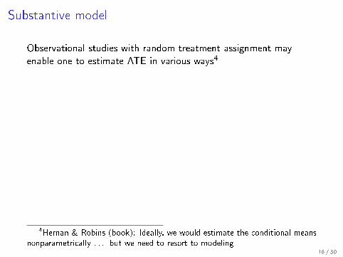
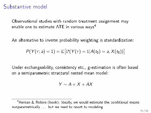
Substantive model

Observational studies with random treatment assignment mayenable one to estimate ATE in various ways4

An alternative to inverse probability weighting is standardization:

P(Y (τ ; a) = 1) = E[P(Y (τ) = 1|A(t0) = a,X (t0))

]Under exchangeability, consistency etc., g-estimation is often basedon a semiparametric structural nested mean model:

Y ∼ A + X + AX

4Hernan & Robins (book): Ideally, we would estimate the conditional meansnonparametrically . . . but we need to resort to modeling

16 / 30

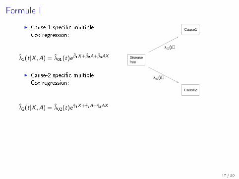
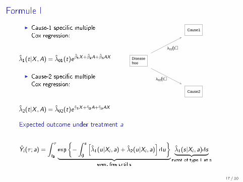
Formule I

I Cause-1 speci�c multipleCox regression:

λ1(t|X ,A) = λ01(t)e β1X+β2A+β3AX


λ2(t|X ,A) = λ02(t)e γ1X+γ2A+γ3AX

Diseasefree

Cause1

Cause2

λ01(t)

λ02(t)

Expected outcome under treatment a

Yi (τ ; a) =

∫ τ

t0

exp

{−∫ s

0

[λ1(u|Xi , a) + λ2(u|Xi , a)

]du

}︸︷︷︸

event-free until s

λ1(s|Xi , a)ds︸︷︷︸event of type 1 at s

17 / 30

Formule I


λ1(t|X ,A) = λ01(t)e β1X+β2A+β3AX


λ2(t|X ,A) = λ02(t)e γ1X+γ2A+γ3AX

Diseasefree

Cause1

Cause2

λ01(t)

λ02(t)

Expected outcome under treatment a

Yi (τ ; a) =

∫ τ

t0

exp

{−∫ s

0

[λ1(u|Xi , a) + λ2(u|Xi , a)

]du

}︸︷︷︸

event-free until s

λ1(s|Xi , a)ds︸︷︷︸event of type 1 at s

17 / 30

Regression method to estimate average e�ects

Backdoor adjustment (Pearl, 1995) aka g-estimation (Robins,1986):

ATE(a, b; τ) =1

n

n∑i=1

[Yi (τ ; a)− Yi (τ ; b)]

Glynn & Quinn5:Further, many versions of the regression estimator for ATE tend to

be quite sensitive to small amounts of misspeci�cation. Given these

de�ciencies, many researchers have opted for methods of estimation

that utilize models for treatment assignment instead of regression

models for the outcome.

5An introduction to the augmented inverse propensity weighted estimator.Political Analysis, 18(1):pp. 36�56, 2010.

18 / 30

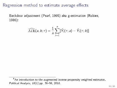
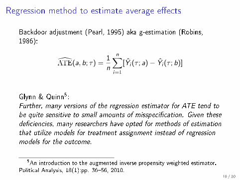
Regression method to estimate average e�ects

Backdoor adjustment (Pearl, 1995) aka g-estimation (Robins,1986):

ATE(a, b; τ) =1

n

n∑i=1

[Yi (τ ; a)− Yi (τ ; b)]

Glynn & Quinn5:Further, many versions of the regression estimator for ATE tend to

be quite sensitive to small amounts of misspeci�cation. Given these

de�ciencies, many researchers have opted for methods of estimation

that utilize models for treatment assignment instead of regression

models for the outcome.

5An introduction to the augmented inverse propensity weighted estimator.Political Analysis, 18(1):pp. 36�56, 2010.

18 / 30

Asymptotics

19 / 30

Notation

Symbol Meaning

T Time to what comes �rst: event or competing riskD Cause of eventC Time of end of followup

T min(T ,C )

D 1{T ≤ C}D

We assume a sample (Xi )i∈{1,...,n} of n independent and identicallydistributed replications of

X = (T , D,X ,A)

Note: under the Cox models, the potential outcome of subject iunder treatment a:

Yi (a; τ) ≈ {cumulative incidence at time τ} = F1(τ |Xi ,A = a)

20 / 30

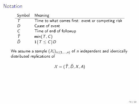
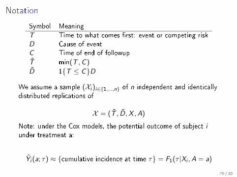
Notation

Symbol Meaning

T Time to what comes �rst: event or competing riskD Cause of eventC Time of end of followup

T min(T ,C )

D 1{T ≤ C}D

We assume a sample (Xi )i∈{1,...,n} of n independent and identicallydistributed replications of

X = (T , D,X ,A)

Note: under the Cox models, the potential outcome of subject iunder treatment a:

Yi (a; τ) ≈ {cumulative incidence at time τ} = F1(τ |Xi ,A = a)

20 / 30

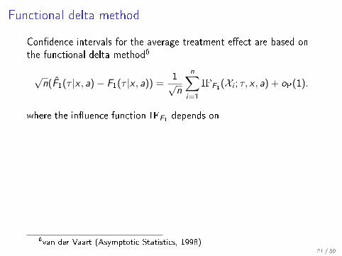
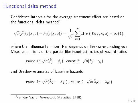
Functional delta method

Con�dence intervals for the average treatment e�ect are based onthe functional delta method6

√n(F1(τ |x , a)− F1(τ |x , a)) =

1√n

n∑i=1

IFF1(Xi ; τ, x , a) + oP(1).

where the in�uence function IFF1 depends on

the corresponding vonMises expansions of the partial likelihood estimates of hazard ratios

cause 1:√n(βj − βj), cause 2:

√n(γj − γj)

and Breslow estimates of baseline hazards

cause 1:√n(λ01 − λ01), cause 2:

√n(λ02 − λ02)

6van der Vaart (Asymptotic Statistics, 1998)21 / 30

Functional delta method

Con�dence intervals for the average treatment e�ect are based onthe functional delta method6

√n(F1(τ |x , a)− F1(τ |x , a)) =

1√n

n∑i=1

IFF1(Xi ; τ, x , a) + oP(1).

where the in�uence function IFF1 depends on the corresponding vonMises expansions of the partial likelihood estimates of hazard ratios

cause 1:√n(βj − βj), cause 2:

√n(γj − γj)

and Breslow estimates of baseline hazards

cause 1:√n(λ01 − λ01), cause 2:

√n(λ02 − λ02)

6van der Vaart (Asymptotic Statistics, 1998)21 / 30

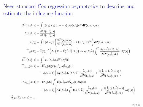
Need standard Cox regression asymptotics to describe and

estimate the in�uence function

S(r)(t, βj , a) =

∫1{t ≤ s ≤ τ,w = a} exp(vβj)v

⊗rdP(s, d , v ,w)

E (t, βj , a) =S(1)(t, βj , a)

S(0)(t, βj , a)

I(βj) =

∫1{d = j}

(S(2)(s, βl ,w)

S(0)(s, βj ,w)− E (s, βj ,w)⊗2

)dP(s, d , v ,w)

IFβj (Xi ) = I(βj)−1(

∆i

(Xi − E (Ti , βj ,Ai )

)− exp(Xi βj)

∫ Ti

0

Xi − E (s, βj ,Ai )

S(0)(s, βj ,Ai )dNa

j (s)

)S(r)(t, βj , a) =

∫ τ

0

exp(Xi βj)X⊗ri dNa

j (t)

IFλ0j,a(Xi ; t) = −IFβj (Xi )E (t, βj , a)λ0j ,a(t)

− 1{Ai = a}(exp(Xi βj)1{t ≤ Ti}

λ0j ,a(t)

S(0)(t, βj , a)+

1{Ti = t, Di = j}

S(0)(Ti , βj ,Ai )

)IFΛ0j,a

(Xi ; t) = −IFβj (Xi )

∫ t

0

E (s, βj , a)λ0j ,a(s)dNaj (s)

− 1{Ai = a}(exp(Xi βj)

∫ t

0

1{s ≤ Ti}λ0j ,a(s)

S(0)(s, βj , a)+

1{Ti ≤ t, Di = j}

S(0)(Ti , βj ,Ai )dNa

j (s)

)IFF1(Xi ; t, x , a) = . . .

22 / 30

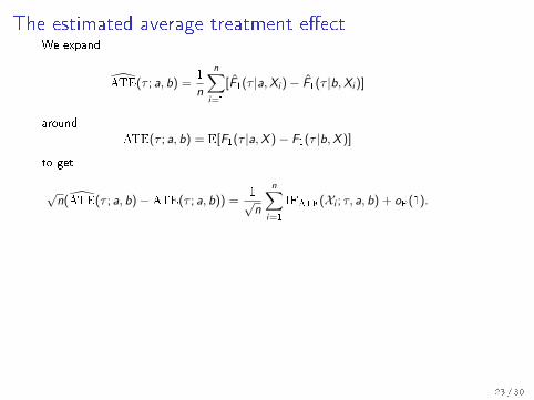
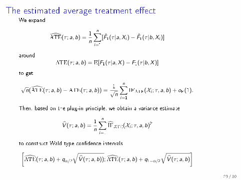
The estimated average treatment e�ectWe expand

ATE(τ ; a, b) =1

n

n∑i=1

[F1(τ |a,Xi )− F1(τ |b,Xi )]

aroundATE(τ ; a, b) = E[F1(τ |a,X )− F1(τ |b,X )]

to get

√n(ATE(τ ; a, b)−ATE(τ ; a, b)) =

1√n

n∑i=1

IFATE(Xi ; τ, a, b) + oP(1).

Then, based on the plug-in principle, we obtain a variance estimate

V (τ ; a, b) =1

n

n∑i=1

IFATE(Xi ; τ, a, b)2

to construct Wald type con�dence intervals[ATE(τ ; a, b) + qα/2

√V (τ ; a, b)); ATE(τ ; a, b) + q1−α/2

√V (τ ; a, b)

]

23 / 30

The estimated average treatment e�ectWe expand

ATE(τ ; a, b) =1

n

n∑i=1

[F1(τ |a,Xi )− F1(τ |b,Xi )]

aroundATE(τ ; a, b) = E[F1(τ |a,X )− F1(τ |b,X )]

to get

√n(ATE(τ ; a, b)−ATE(τ ; a, b)) =

1√n

n∑i=1

IFATE(Xi ; τ, a, b) + oP(1).

Then, based on the plug-in principle, we obtain a variance estimate

V (τ ; a, b) =1

n

n∑i=1

IFATE(Xi ; τ, a, b)2

to construct Wald type con�dence intervals[ATE(τ ; a, b) + qα/2

√V (τ ; a, b)); ATE(τ ; a, b) + q1−α/2

√V (τ ; a, b)

]23 / 30

Software

24 / 30

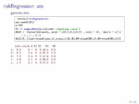
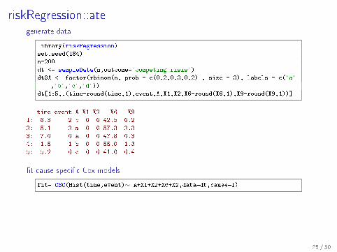
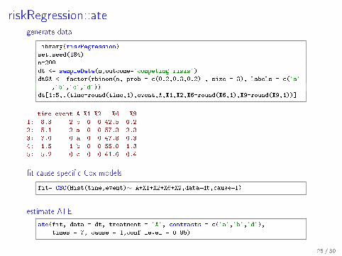
riskRegression::ategenerate data

library(riskRegression)

set.seed(184)

n=200

dt <- sampleData(n,outcome="competing.risks")

dt$A <- factor(rbinom(n, prob = c(0.2,0.3,0.2) , size = 3), labels = c("a"

,"b","c","d"))

dt[1:5,.(time=round(time,1),event,A,X1,X2,X6=round(X6,1),X9=round(X9,1))]

time event A X1 X2 X6 X9

1: 8.3 2 b 0 0 42.5 0.2

2: 5.1 2 a 0 0 57.3 2.3

3: 7.0 0 a 0 0 47.8 0.3

4: 1.5 1 b 0 0 55.0 -1.3

5: 5.2 0 c 0 0 41.6 0.4

�t cause-speci�c Cox models

fit= CSC(Hist(time,event)∼ A+X1+X2+X6+X9,data=dt,cause=1)

estimate ATE

ate(fit, data = dt, treatment = "A", contrasts = c("a","b","d"),

times = 7, cause = 1,conf.level = 0.95)

25 / 30



set.seed(184)

n=200



,"b","c","d"))



1: 8.3 2 b 0 0 42.5 0.2

2: 5.1 2 a 0 0 57.3 2.3

3: 7.0 0 a 0 0 47.8 0.3

4: 1.5 1 b 0 0 55.0 -1.3

5: 5.2 0 c 0 0 41.6 0.4



estimate ATE



25 / 30



set.seed(184)

n=200



,"b","c","d"))



1: 8.3 2 b 0 0 42.5 0.2

2: 5.1 2 a 0 0 57.3 2.3

3: 7.0 0 a 0 0 47.8 0.3

4: 1.5 1 b 0 0 55.0 -1.3

5: 5.2 0 c 0 0 41.6 0.4



estimate ATE



25 / 30

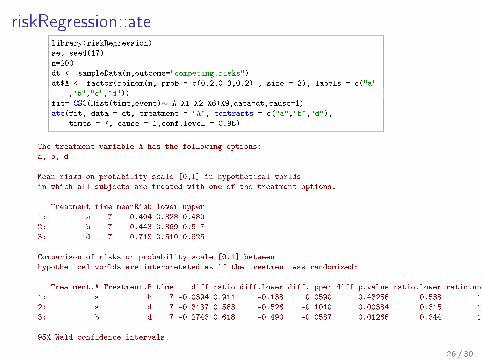
riskRegression::atelibrary(riskRegression)

set.seed(17)

n=200



,"b","c","d"))




The treatment variable A has the following options:

a, b, d

Mean risks on probability scale [0,1] in hypothetical worlds

in which all subjects are treated with one of the treatment options:

Treatment time meanRisk lower upper

1: a 7 0.404 0.328 0.480

2: b 7 0.443 0.369 0.517

3: d 7 0.718 0.510 0.925

Comparison of risks on probability scale [0,1] between

hypothetical worlds are interpretated as if the treatment was randomized:

Treatment.A Treatment.B time diff ratio diff.lower diff.upper diff.p.value ratio.lower ratio.upper ratio.p.value

1: a b 7 -0.0394 0.911 -0.138 0.0590 0.43256 0.538 1.54 0.7294

2: a d 7 -0.3137 0.563 -0.526 -0.1010 0.00384 0.315 1.01 0.0521

3: b d 7 -0.2743 0.618 -0.490 -0.0587 0.01266 0.344 1.11 0.1059

95% Wald confidence intervals.

26 / 30

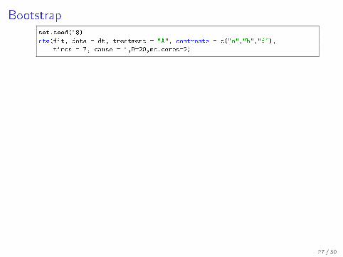
Bootstrapset.seed(18)


times = 7, cause = 1,B=20,mc.cores=2)

27 / 30

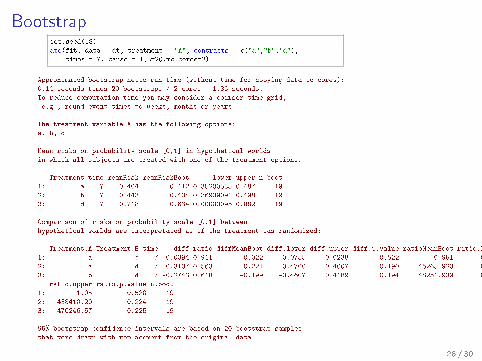
Bootstrapset.seed(18)


times = 7, cause = 1,B=20,mc.cores=2)

Approximated bootstrap netto run time (without time for copying data to cores):

0.14 seconds times 20 bootstraps / 2 cores = 1.36 seconds.

To reduce computation time you may consider a coarser time grid,

e.g., round event times to weeks, months or years.

The treatment variable A has the following options:

a, b, d

Mean risks on probability scale [0,1] in hypothetical worlds

in which all subjects are treated with one of the treatment options:

Treatment time meanRisk meanRiskBoot lower upper n.boot

1: a 7 0.404 0.412 0.35200585 0.487 19

2: b 7 0.443 0.434 0.36939091 0.498 19

3: d 7 0.718 0.634 0.00000095 0.882 19

Comparison of risks on probability scale [0,1] between

hypothetical worlds are interpretated as if the treatment was randomized:

Treatment.A Treatment.B time diff ratio diffMeanBoot diff.lower diff.upper diff.p.value ratioMeanBoot ratio.lower

1: a b 7 -0.0394 0.911 -0.022 -0.0755 0.0238 0.522 0.951 0.834

2: a d 7 -0.3137 0.563 -0.221 -0.4700 0.4007 0.190 45265.923 0.462

3: b d 7 -0.2743 0.618 -0.199 -0.4607 0.4189 0.194 48251.939 0.478

ratio.upper ratio.p.value n.boot

1: 1.05 0.520 19

2: 438410.20 0.224 19

3: 470246.57 0.225 19

95% bootstrap confidence intervals are based on 20 bootstrap samples

that were drawn with replacement from the original data.

28 / 30

Discussion

I Causal inference is still 'sexy' in many research groups

I It is important that one can imagine a randomized trial

I The hype has reached pharmacoepidemiologists who oftenhave large data sets, issues with time, and interesting problems

I Absolute risks can be estimated using cause-speci�c Coxregression 7

Modelling issues

I choice of τ

I compliance/intention to treat

I strati�ed baseline hazards

I interactions

7Benichou & Gail (1990)29 / 30

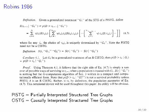
Robins 1986

PISTG = Partially Interpreted Structured Tree GraphsCISTG = Causally Interpreted Structured Tree Graphs

30 / 30

Documents

The g-formula for competing risks - kupublicifsv.sund.ku.dk/~tag/download/ulm-presentation-2017.pdf · The g-formula for competing risks Brice Ozenne & Thomas Alexander Gerds Biostatistics,