The Future of Automotive Localization Algorithms: Available, reliable, and scalable

localization: Anywhere and anytime

Rickard Karlsson and Fredrik Gustafsson

Journal Article

N.B.: When citing this work, cite the original article.

©2016 IEEE. Personal use of this material is permitted. However, permission to reprint/republish this material for advertising or promotional purposes or for creating new collective works for resale or redistribution to servers or lists, or to reuse any copyrighted component of this work in other works must be obtained from the IEEE.

Rickard Karlsson and Fredrik Gustafsson, The Future of Automotive Localization Algorithms: Available, reliable, and scalable localization: Anywhere and anytime, IEEE signal processing magazine (Print), 2017. 34(2), pp.60-69. http://dx.doi.org/10.1109/MSP.2016.2637418 Postprint available at: Linköping University Electronic Press

http://urn.kb.se/resolve?urn=urn:nbn:se:liu:diva-135786

1

The Future of Automotive Localization AlgorithmsRickard Karlsson and Fredrik Gustafsson

Department of Electrical EngineeringLinkoping University, Linkoping Sweden

E-mail: {rickard, fredrik}@isy.liu.se

Abstract—Most navigation systems today rely on global navi-gation satellite systems (GNSS), including navigation in cars. Withsupport from odometry and inertial sensors, this is a sufficientlyaccurate and robust solution, but there are future demands.Autonomous cars require higher accuracy and integrity. Using thecar as a sensor probe for road conditions in cloud-based servicesalso sets other kind of requirements. The Internet of Thingsconcept require stand-alone solutions without access to vehicledata. Our vision is a future with both in-vehicle localizationalgorithms and after market products, where the position iscomputed with high accuracy in GNSS-denied environments. Wepresent a localization approach based on a prior that vehiclesspend most time on the road, with odometer as the primaryinput. When wheel speeds are not available, we present anapproach solely based on inertial sensors, which also can beused as a speedometer. The map information is included in aBayesian setting using the particle filter, rather than standardmap matching. In extensive experiments the performance withoutGNSS is shown to have basically the same quality as utilizing aGNSS sensor. Several topics are treated: virtual measurements,dead reckoning, inertial sensor information, indoor-positioning,off-road driving, and multi-level positioning.

Index Terms—Localization, map-aided positioning, particlefilter, velocity estimation.

I. INTRODUCTION

Today’s positioning systems are intended for humansrather than machines. The position is presented

and used for instructions innavigation systems, or forreporting vehicle data, alsoincluding emergency acci-dent location. We refer tothe area as localization al-gorithms for several rea-sons. First, the word al-gorithm indicates softwaredevelopment. Already todaythere is sufficient informa-tion at hand, in terms of sen-sors and databases to makea leap in performance com-pared to GNSS-based solu-tions. Second, localization

is not a system, it is rather a service required by many systems.Third, the term navigation is avoided since this is only oneapplication of localization algorithms. Fourth, localization issometimes a more appropriate term than positioning, sincea true longitude and latitude position is of no value unless

the map and situational awareness have the same absoluteaccuracy.

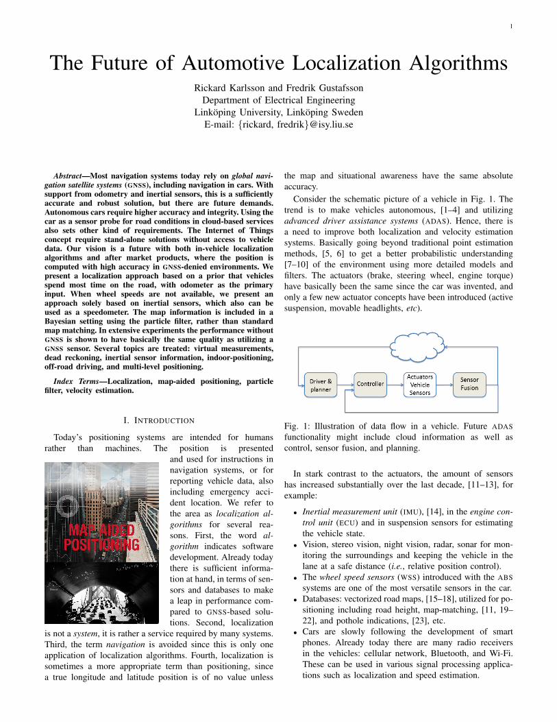
Consider the schematic picture of a vehicle in Fig. 1. Thetrend is to make vehicles autonomous, [1–4] and utilizingadvanced driver assistance systems (ADAS). Hence, there isa need to improve both localization and velocity estimationsystems. Basically going beyond traditional point estimationmethods, [5, 6] to get a better probabilistic understanding[7–10] of the environment using more detailed models andfilters. The actuators (brake, steering wheel, engine torque)have basically been the same since the car was invented, andonly a few new actuator concepts have been introduced (activesuspension, movable headlights, etc).

Fig. 1: Illustration of data flow in a vehicle. Future ADASfunctionality might include cloud information as well ascontrol, sensor fusion, and planning.

In stark contrast to the actuators, the amount of sensorshas increased substantially over the last decade, [11–13], forexample:

• Inertial measurement unit (IMU), [14], in the engine con-trol unit (ECU) and in suspension sensors for estimatingthe vehicle state.

• Vision, stereo vision, night vision, radar, sonar for mon-itoring the surroundings and keeping the vehicle in thelane at a safe distance (i.e., relative position control).

• The wheel speed sensors (WSS) introduced with the ABSsystems are one of the most versatile sensors in the car.

• Databases: vectorized road maps, [15–18], utilized for po-sitioning including road height, map-matching, [11, 19–22], and pothole indications, [23], etc.

• Cars are slowly following the development of smartphones. Already today there are many radio receiversin the vehicles: cellular network, Bluetooth, and Wi-Fi.These can be used in various signal processing applica-tions such as localization and speed estimation.

2

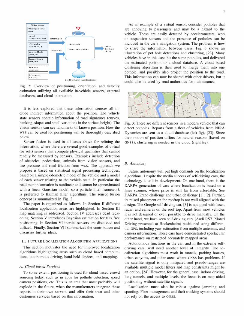
Fig. 2: Overview of positioning, orientation, and velocityestimation utilizing all available in-vehicle sensors, externaldatabases, and cloud interaction.

It is less explored that these information sources all in-clude indirect information about the position. The vehiclestate sensors contain information of road signatures (curves,banking, slopes and small variations in the surface height). Thevision sensors can see landmarks of known position. How theWSS can be used for positioning will be thoroughly describedbelow.

Sensor fusion is used in all cases above for refining theinformation, where there are several good examples of virtual(or soft) sensors that compute physical quantities that cannotreadily be measured by sensors. Examples include detectionof obstacles, pedestrians, animals from vision sensors, andtire pressure and road friction from WSS. The approach wepropose is based on statistical signal processing techniques,based on a simple odometric model of the vehicle and a modelof each sensor relating to the vehicle state. In particular theroad map information is nonlinear and cannot be approximatedwith a linear Gaussian model, so a particle filter frameworkis preferred to Kalman filter algorithms. The sensor fusionconcept is summarized in Fig. 2.

The paper is organized as follows. In Section II differentlocalization application areas are highlighted. In Section IIImap matching is addressed. Section IV addresses dead reck-oning. Section V introduces Bayesian estimation for GPS freepositioning. In Section VI inertial sensors are discussed andutilized. Finally, Section VII summarizes the contribution anddiscusses further ideas.

II. FUTURE LOCALIZATION ALGORITHM APPLICATIONS

This section motivates the need for improved localizationalgorithms highlighting areas such as cloud based computa-tions, autonomous driving, hand-held devices, and mapping.

A. Cloud-based Services

To some extent, positioning is used for cloud based crowdsourcing today, such as in apps for pothole detection, speedcamera positions, etc. This is an area that most probably willexplode in the future, when the manufacturers integrate thesereports in their own servers, and offer their own and othercustomers services based on this information.

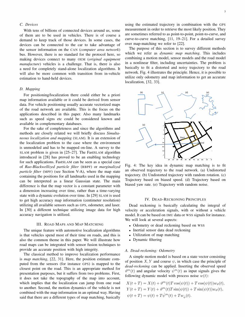
As an example of a virtual sensor, consider potholes thatare annoying to passengers and may be a hazard to thevehicle. These are easily detected by accelerometers, WSSor suspension sensors and the presence of potholes can beincluded in the car’s navigation system. The problem is howto share the information between users. Fig. 3 shows anillustration of pot hole detections and clustering, [23]. Manyvehicles have in this case hit the same potholes, and deliveredthe estimated position to a cloud database. A cloud basedclustering algorithm is then used to merge them into onepothole, and possibly also project the position to the road.This information can now be shared with other drivers, but itcould also be used by road authorities for maintenance.

Fig. 3: There are different sensors in a modern vehicle that candetect potholes. Reports from a fleet of vehicles from NIRADynamics are sent to a cloud database (left fig), [23]. Sincetheir notion of position differs for natural reasons (based onGNSS), clustering is needed in the cloud (right fig).

B. Autonomy

Future autonomy will put high demands on the localizationalgorithms. Despite the media success of self-driving cars, thetechnology is still in development. On one hand, there is theDARPA generation of cars where localization is based on alaser scanner, whose price is still far from affordable, SeeDARPA Grand challenge and urban challenge [1], [2]. Further,its raised placement on the rooftop is not well aligned with thedesign. The Google self-driving car, [3] is equipped with laser,radar, and cameras on the roof top. Apart from most vehiclesit is not designed or even possible to drive manually. On theother hand, we have seen self-driving cars (Audi RS7 PilotedDriving presented at Hockenheim) positioned using differen-tial GPS, including yaw estimation from multiple antennas, andcamera information. These cars have demonstrated spectacularperformance on restricted accurately mapped areas.

Autonomous functions in the car, and in the extreme self-driving cars, will need another level of integrity. The lo-calization algorithms must work in tunnels, parking houses,urban canyons, and other areas where GNSS has problems. Ifthe satellite signal is only mitigated and pseudo-ranges areavailable multiple model filters and map constraints might bean option, [24]. However, for the general case: indoor driving,long tunnels, and multiple levels, the focus is on map aidedpositioning without satellite signals.

Localization must also be robust against jamming andspoofing. Fleet management and theft tracking systems shouldnot rely on the access to GNSS.

3

C. Devices

With tens of billions of connected devices around us, someof them are to be used in vehicles. There is of course ademand to keep track of those devices. In some cases, thedevices can be connected to the car to take advantage ofthe sensor information on the CAN (computer area network)bus. However, there is no standard for the protocol here, somaking devices connect to many OEM (original equipmentmanufacture) vehicles is a challenge. That is, there is alsoa need for completely stand-alone localization algorithms. Itwill also be more common with transition from in-vehicleestimation to hand-held devices.

D. Mapping

For positioning/localization there could either be a priorimap information available or it could be derived from sensordata. For vehicle positioning usually accurate vectorized mapsof the road network are available. This is the focus on theapplications described in this paper. Also many landmarkssuch as speed signs etc could be considered known andavailable in complementary databases.

For the sake of completeness and since the algorithms andmethods are closely related we will briefly discuss Simulta-neous localization and mapping (SLAM). It is an extension ofthe localization problem to the case where the environmentis unmodeled and has to be mapped on-line. A survey to theSLAM problem is given in [25–27]. The FastSLAM algorithmintroduced in [28] has proved to be an enabling technologyfor such applications. FastSLAM can be seen as a special caseof Rao-Blackwellized particle filter (RBPF) or marginalizedparticle filter (MPF) (see Section V-A), where the map statecontaining the positions for all landmarks used in the mappingcan be interpreted as a linear Gaussian state. The maindifference is that the map vector is a constant parameter witha dimension increasing over time, rather than a time-varyingstate with a dynamic evolution over time. In [29] SLAM is usedto get high accuracy map information (centimeter resolution)utilizing all available sensors such as GPS, odometer, and laser.In [30] a different technique utilizing image data for highaccuracy navigation is utilized.

III. ROAD MAPS AND MAP MATCHING

The unique feature with automotive localization algorithmsis that vehicles spend most of their time on roads, and this isalso the common theme in this paper. We will illustrate howroad maps can be integrated with sensor fusion techniques toprovide an accurate position with high integrity.

The classical method to improve localization performanceis map matching, [22, 31]. Here, the position estimate com-puted from the sensors (for instance GPS) is mapped to theclosest point on the road. This is an appropriate method forpresentation purposes, but it suffers from two problems. First,it does not take the topography of the map into account,which implies that the localization can jump from one roadto another. Second, the motion dynamics of the vehicle is notcombined with the map information in an optimal way. Havingsaid that there are a different types of map matching, basically

using the estimated trajectory in combination with the GPSmeasurement in order to retrieve the most likely position. Theyare sometimes referred to as point-to-point, point-to-curve, andcurve-to-curve matching, [11, 19–21]. For a detailed surveyover map-matching we refer to [22].

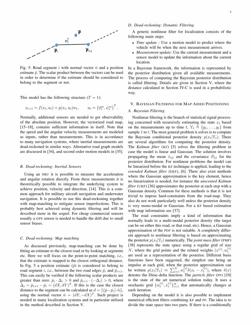
The purpose of this section is to survey different methodswhich we refer as dynamic map matching. This includescombining a motion model, sensor models and the road modelin a nonlinear filter, including uncertainties. The problem isbasically to fit a distorted and noisy trajectory to the roadnetwork. Fig. 4 illustrates the principle. Hence, it is possible toutilize only odometry and map information to get an accuratelocalization, [32, 33].

Start

End

(b) (c) (d) (e)

(a)

Fig. 4: The key idea in dynamic map matching is to fitan observed trajectory to the road network. (a) Undistortedtrajectory. (b) Undistorted trajectory with random rotation. (c)Trajectory based on biased speed. (d) Trajectory based onbiased yaw rate. (e) Trajectory with random noise.

IV. DEAD-RECKONING PRINCIPLES

Dead reckoning is basically calculating the integral ofvelocity or acceleration signals, with or without a vehiclemodel. It can be based on IMU data or WSS signals for instance.We will look at several aspects:• Odometry or dead reckoning based on WSS• Inertial sensor data dead reckoning• Utilization of map matching• Dynamic filtering

A. Dead-reckoning: Odometry

A simple motion model is based on a state vector consistingof position X,Y and course ψ, in which case the principle ofdead-reckoning can be applied. Inserting the observed speedϑm(t) and angular velocity ψm(t) as input signals gives thefollowing dynamic model with process noise w(t):

X(t+ T ) = X(t) + ϑm(t)T cos(ψ(t)) + T cos(ψ(t))wϑ(t),

Y (t+ T ) = Y (t) + ϑm(t)T sin(ψ(t)) + T sin(ψ(t))wϑ(t),

ψ(t+ T ) = ψ(t) + T ψm(t) + Twψ(t).

4

Fig. 5: Road segment i with normal vector n and a positionestimate p. The scalar product between the vectors can be usedin order to determine if the estimate should be considered tobelong to the segment or not.

This model has the following structure (T = 1):

xt+1 = f(xt, ut) + g(xt, ut)wt, ut =(ϑmt , ψ

mt

)T.

Normally, additional sensors are needed to get observabilityof the absolute position. However, the vectorized road map,[15–18], contains sufficient information in itself. Note thatthe speed and the angular velocity measurements are modeledas inputs, rather than measurements. This is in accordanceto many navigation systems, where inertial measurements aredead-reckoned in similar ways. Alternative road graph modelsare discussed in [34], and second order motion models in [35].

B. Dead-reckoning: Inertial Sensors

Using an IMU it is possible to measure the accelerationand angular rotation directly. From these measurements it istheoretically possible to integrate the underlying system toachieve position, velocity and direction, [14]. This is a com-mon approach for military aircraft navigation and underwaternavigation. It is possible to use this dead-reckoning togetherwith map-matching to mitigate sensor imperfections. This isprobably best achieved using dynamic filtering and will bedescribed more in the sequel. For cheap commercial sensorsusually a GPS sensor is needed to handle the drift due to smallsensor biases.

C. Dead-reckoning: Map matching

As discussed previously, map-matching can be done byfitting an estimate to the closest road or by looking at segmentsetc. Here we will focus on the point-to-point matching, i.e.,that the estimate is mapped to the closest orthogonal distance.In Fig. 5 a position estimate (p) is considered to belong toroad segment i, i.e., between the two road edges pi and pi+1.This can easily be verified if the following scalar products aregreater than zero: pi · ∆i > 0 and pi+1 · (−∆i) > 0, where∆i = pi+1 − pi = (dX, dY )T . If this is the case the closestdistance to the segment can be calculated as d = ||(p−pi)·n||,using the normal vector n = (dY,−dX)T . Such project isneeded in many localization systems and in particular utilizedin the method described in Section V.

D. Dead-reckoning: Dynamic Filtering

A generic nonlinear filter for localization consists of thefollowing main steps:• Time update : Use a motion model to predict where the

vehicle will be when the next measurement arrives.• Measurement update: Use the current measurement and a

sensor model to update the information about the currentlocation.

In a Bayesian framework, the information is represented bythe posterior distribution given all available measurements.The process of computing the Bayesian posterior distributionis called filtering. Details are given in Section V, where thedistance calculated in Section IV-C is used in a probabilisticway.

V. BAYESIAN FILTERING FOR MAP AIDED POSITIONING

A. Bayesian Filtering

Nonlinear filtering is the branch of statistical signal process-ing concerned with recursively estimating the state xt basedon the measurements up to time t, Yt , {y1, . . . , yt} fromsample 1 to t. The most general problem it solves is to computethe Bayesian conditional posterior density p(xt|Yt). Thereare several algorithms for computing the posterior density.The Kalman filter (KF) [5] solves the filtering problem incase the model is linear and Gaussian. The solution involvespropagating the mean xt|t and the covariance Pt|t for theposterior distribution. For nonlinear problems the model canbe linearized before the KF technique is applied, leading to theextended Kalman filter (EKF), [6]. There also exist methodswhere the Gaussian approximation is the key element, henceno linearization is needed, for instance the unscented Kalmanfilter (UKF) [36] approximates the posterior at each step with aGaussian density. Common for these methods is that it is nottrivial to impose hard-constraints from the road-map. Theyalso do not work particularly well unless the posterior densityis very mono-modal or Gaussian. For a KF based estimationwith map information see [37].

The road constraints imply a kind of information thatnormally leads to a multi-modal posterior density (the targetcan be on either this road, or that road, etc). Hence, a Gaussianapproximation of the PDF is not suitable. A completely differ-ent approach to nonlinear filtering is based on approximatingthe posterior p(xt|Yt) numerically. The point mass filter (PMF)[38] represents the state space using a regular grid of sizeN , where the grid points and the related weights (x(i), w

(i)t

are used as a representation of the posterior. Different basisfunctions have been suggested, the simplest one being animpulse at each grid, when the posterior approximation canbe written p(xt|Yt) ≈

∑Ni=1 w

(i)t δ(xt − x

(i)t ), where δ(x)

denotes the Dirac-delta function. The particle filter (PF) [10]is the state of the art numerical solution today. It uses astochastic grid {w(i)

t , x(i)t }Ni=1 that automatically changes at

each iteration.Depending on the model it is also possible to implement

numerical efficient filters combining KF and PF. The idea is todivide the state space into two parts. If there is a conditionally

5

linear Gaussian substructure with this partition, the KF can beutilized for that part and the PF for the other part. This isreferred to as the Rao-Blackwellized particle filter (RBPF) orthe marginalized particle filter (MPF), [7–9, 39–41] The RBPFimproves the performance when a linear Gaussian substructureis present, e.g., in various map based positioning applicationsand target tracking applications as shown in [41].

The map aided positioning algorithm based on the particlefilter is summarized in Alg. 1.

Algorithm 1 Particle Filter for Map Aided PositioningGiven the system

xt+1 = f(xt) + wt

yt = h(xt) + et

1: Initialization: For i = 1, . . . , N , x0|−1 ∼ px(i)0

(x0) andset t = 0.

2: PF measurement update: For i = 1, . . . , N , evaluate theimportance weights ω(i)

t = p(yt|x(i)t|t ,Yt−1), and normal-

ize ω(i)t = ω

(i)t /

∑j ω

(j)t using map information.

3: Resample N particles with replacement:Pr(x

(i)t|t = x

(j)t|t−1) = ω

(j)t .

3: PF time update: For i = 1, . . . , N predict new particlesx(i)t+1|t ∼ p(xt+1|t|X

(i)t ,Yt).

4: Increase time and repeat from step 2.

B. Particle Filter Based Map Aided Positioning

In this section the map aided positioning (MAP) method isfirst illustrated on experimental data. After that the crucial mapbased observation is described in detail. Finally, the algorithmperformance is presented on 10 experiments conducted in thesame driving scenario (see Fig. 7).

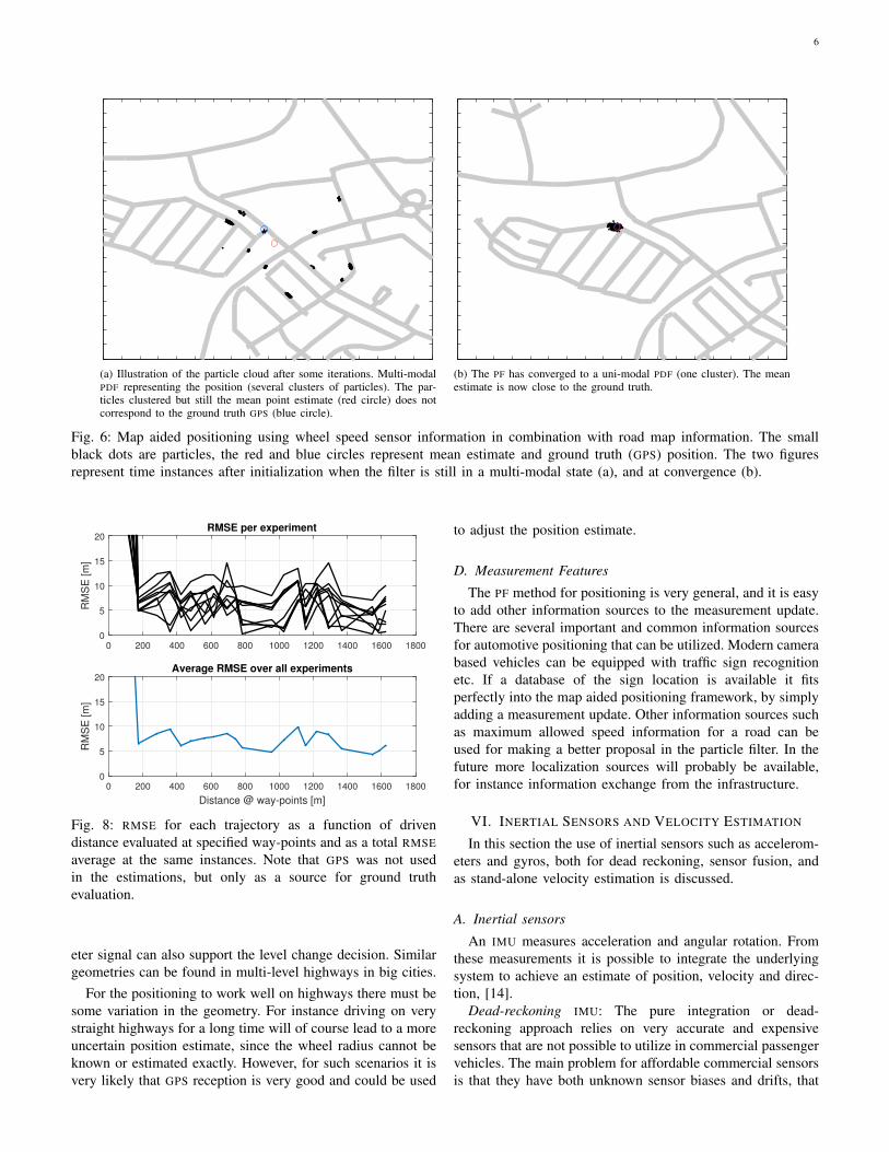
1) MAP illustrations: In Fig. 6 the map aided positioningusing wheel speed information and road map information isdemonstrated, where GPS information is used as a ground truthreference only. For other map aided positioning applicationssee for instance [42–48]. First the PF is initialized in thevicinity of the GPS position. The initial distribution is chosenuniformly on road segments in a region around the GPSfix. Particles are allowed slightly off-road to handle off-roadsituations and small map errors. In Fig. 6 (a) the algorithm hasbeen active for some time. As seen, the PDF is highly multi-modal (several clusters of particles). Note that the PF algorithmuses only wheel speeds from the CAN-bus and that the GPSis only used to evaluate the ground truth. In Fig. 6 (b), afteryet some turns, the filter has converged and the mean estimate(red circle) is close to the true position (blue circle).

2) MAP algorithm: As discussed in Section IV-C mapmatching can be used to fit an estimate to the closest roadsegment. In this section we will focus on the PF implemen-tation, so for each particle it is crucial to find the closestroad segment. The generic PF algorithm is used for mapaided positioning. The road map is used as a virtual sensor,so there is not an actual measurement function. Instead theclosest distance to every road segment is evaluated for each

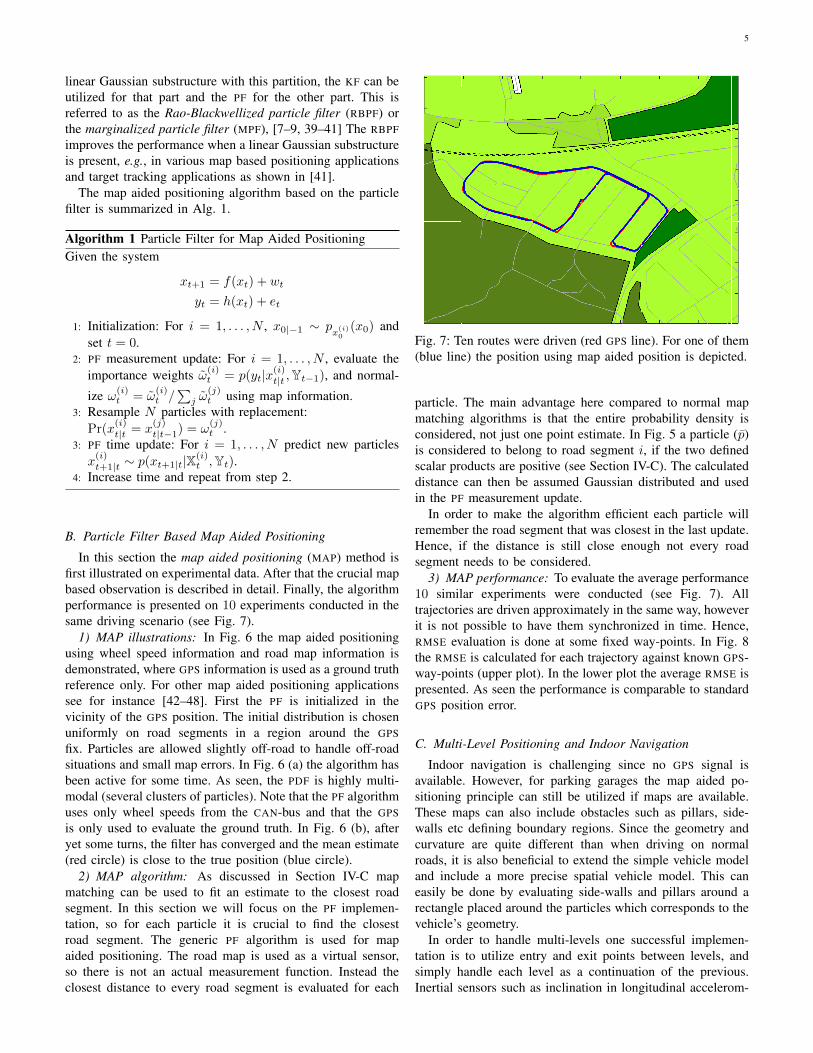
Fig. 7: Ten routes were driven (red GPS line). For one of them(blue line) the position using map aided position is depicted.

particle. The main advantage here compared to normal mapmatching algorithms is that the entire probability density isconsidered, not just one point estimate. In Fig. 5 a particle (p)is considered to belong to road segment i, if the two definedscalar products are positive (see Section IV-C). The calculateddistance can then be assumed Gaussian distributed and usedin the PF measurement update.

In order to make the algorithm efficient each particle willremember the road segment that was closest in the last update.Hence, if the distance is still close enough not every roadsegment needs to be considered.

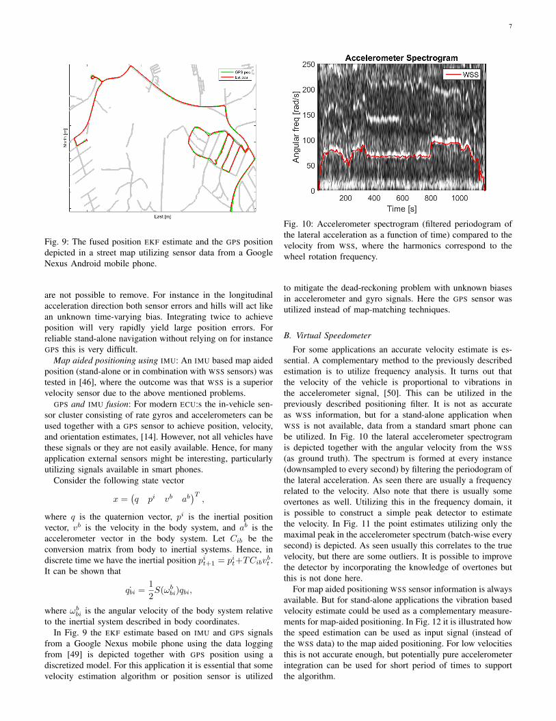
3) MAP performance: To evaluate the average performance10 similar experiments were conducted (see Fig. 7). Alltrajectories are driven approximately in the same way, howeverit is not possible to have them synchronized in time. Hence,RMSE evaluation is done at some fixed way-points. In Fig. 8the RMSE is calculated for each trajectory against known GPS-way-points (upper plot). In the lower plot the average RMSE ispresented. As seen the performance is comparable to standardGPS position error.

C. Multi-Level Positioning and Indoor Navigation

Indoor navigation is challenging since no GPS signal isavailable. However, for parking garages the map aided po-sitioning principle can still be utilized if maps are available.These maps can also include obstacles such as pillars, side-walls etc defining boundary regions. Since the geometry andcurvature are quite different than when driving on normalroads, it is also beneficial to extend the simple vehicle modeland include a more precise spatial vehicle model. This caneasily be done by evaluating side-walls and pillars around arectangle placed around the particles which corresponds to thevehicle’s geometry.

In order to handle multi-levels one successful implemen-tation is to utilize entry and exit points between levels, andsimply handle each level as a continuation of the previous.Inertial sensors such as inclination in longitudinal accelerom-

6

(a) Illustration of the particle cloud after some iterations. Multi-modalPDF representing the position (several clusters of particles). The par-ticles clustered but still the mean point estimate (red circle) does notcorrespond to the ground truth GPS (blue circle).

(b) The PF has converged to a uni-modal PDF (one cluster). The meanestimate is now close to the ground truth.

Fig. 6: Map aided positioning using wheel speed sensor information in combination with road map information. The smallblack dots are particles, the red and blue circles represent mean estimate and ground truth (GPS) position. The two figuresrepresent time instances after initialization when the filter is still in a multi-modal state (a), and at convergence (b).

0 200 400 600 800 1000 1200 1400 1600 1800

RM

SE

[m

]

0

5

10

15

20RMSE per experiment

Distance @ way-points [m]

0 200 400 600 800 1000 1200 1400 1600 1800

RM

SE

[m

]

0

5

10

15

20Average RMSE over all experiments

Fig. 8: RMSE for each trajectory as a function of drivendistance evaluated at specified way-points and as a total RMSEaverage at the same instances. Note that GPS was not usedin the estimations, but only as a source for ground truthevaluation.

eter signal can also support the level change decision. Similargeometries can be found in multi-level highways in big cities.

For the positioning to work well on highways there must besome variation in the geometry. For instance driving on verystraight highways for a long time will of course lead to a moreuncertain position estimate, since the wheel radius cannot beknown or estimated exactly. However, for such scenarios it isvery likely that GPS reception is very good and could be used

to adjust the position estimate.

D. Measurement Features

The PF method for positioning is very general, and it is easyto add other information sources to the measurement update.There are several important and common information sourcesfor automotive positioning that can be utilized. Modern camerabased vehicles can be equipped with traffic sign recognitionetc. If a database of the sign location is available it fitsperfectly into the map aided positioning framework, by simplyadding a measurement update. Other information sources suchas maximum allowed speed information for a road can beused for making a better proposal in the particle filter. In thefuture more localization sources will probably be available,for instance information exchange from the infrastructure.

VI. INERTIAL SENSORS AND VELOCITY ESTIMATION

In this section the use of inertial sensors such as accelerom-eters and gyros, both for dead reckoning, sensor fusion, andas stand-alone velocity estimation is discussed.

A. Inertial sensors

An IMU measures acceleration and angular rotation. Fromthese measurements it is possible to integrate the underlyingsystem to achieve an estimate of position, velocity and direc-tion, [14].

Dead-reckoning IMU: The pure integration or dead-reckoning approach relies on very accurate and expensivesensors that are not possible to utilize in commercial passengervehicles. The main problem for affordable commercial sensorsis that they have both unknown sensor biases and drifts, that

7

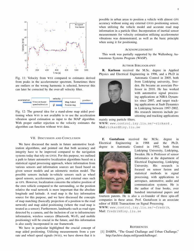
Fig. 9: The fused position EKF estimate and the GPS positiondepicted in a street map utilizing sensor data from a GoogleNexus Android mobile phone.

are not possible to remove. For instance in the longitudinalacceleration direction both sensor errors and hills will act likean unknown time-varying bias. Integrating twice to achieveposition will very rapidly yield large position errors. Forreliable stand-alone navigation without relying on for instanceGPS this is very difficult.

Map aided positioning using IMU: An IMU based map aidedposition (stand-alone or in combination with WSS sensors) wastested in [46], where the outcome was that WSS is a superiorvelocity sensor due to the above mentioned problems.

GPS and IMU fusion: For modern ECU:s the in-vehicle sen-sor cluster consisting of rate gyros and accelerometers can beused together with a GPS sensor to achieve position, velocity,and orientation estimates, [14]. However, not all vehicles havethese signals or they are not easily available. Hence, for manyapplication external sensors might be interesting, particularlyutilizing signals available in smart phones.

Consider the following state vector

x =(q pi vb ab

)T,

where q is the quaternion vector, pi is the inertial positionvector, vb is the velocity in the body system, and ab is theaccelerometer vector in the body system. Let Cib be theconversion matrix from body to inertial systems. Hence, indiscrete time we have the inertial position pit+1 = pit+TCibv

bt .

It can be shown that

˙qbi =1

2S(ωbbi)qbi,

where ωbbi is the angular velocity of the body system relativeto the inertial system described in body coordinates.

In Fig. 9 the EKF estimate based on IMU and GPS signalsfrom a Google Nexus mobile phone using the data loggingfrom [49] is depicted together with GPS position using adiscretized model. For this application it is essential that somevelocity estimation algorithm or position sensor is utilized

Fig. 10: Accelerometer spectrogram (filtered periodogram ofthe lateral acceleration as a function of time) compared to thevelocity from WSS, where the harmonics correspond to thewheel rotation frequency.

to mitigate the dead-reckoning problem with unknown biasesin accelerometer and gyro signals. Here the GPS sensor wasutilized instead of map-matching techniques.

B. Virtual Speedometer

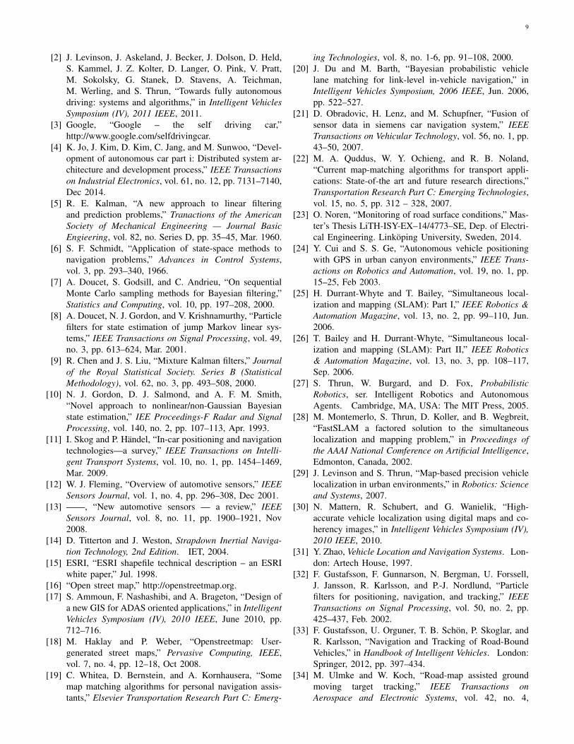
For some applications an accurate velocity estimate is es-sential. A complementary method to the previously describedestimation is to utilize frequency analysis. It turns out thatthe velocity of the vehicle is proportional to vibrations inthe accelerometer signal, [50]. This can be utilized in thepreviously described positioning filter. It is not as accurateas WSS information, but for a stand-alone application whenWSS is not available, data from a standard smart phone canbe utilized. In Fig. 10 the lateral accelerometer spectrogramis depicted together with the angular velocity from the WSS(as ground truth). The spectrum is formed at every instance(downsampled to every second) by filtering the periodogram ofthe lateral acceleration. As seen there are usually a frequencyrelated to the velocity. Also note that there is usually someovertones as well. Utilizing this in the frequency domain, itis possible to construct a simple peak detector to estimatethe velocity. In Fig. 11 the point estimates utilizing only themaximal peak in the accelerometer spectrum (batch-wise everysecond) is depicted. As seen usually this correlates to the truevelocity, but there are some outliers. It is possible to improvethe detector by incorporating the knowledge of overtones butthis is not done here.

For map aided positioning WSS sensor information is alwaysavailable. But for stand-alone applications the vibration basedvelocity estimate could be used as a complementary measure-ments for map-aided positioning. In Fig. 12 it is illustrated howthe speed estimation can be used as input signal (instead ofthe WSS data) to the map aided positioning. For low velocitiesthis is not accurate enough, but potentially pure accelerometerintegration can be used for short period of times to supportthe algorithm.

8

Fig. 11: Velocity from WSS compared to estimates derivedfrom peaks in the accelerometer spectrum. Sometimes thereare outliers or the wrong harmonic is selected, however thiscan later be corrected by the over-all velocity filter.

Fig. 12: The general idea for a stand-alone map aided posi-tioning when WSS is not available is to use the accelerationvibration speed estimation as input to the MAP algorithm.With proper outlier rejection to the velocity estimates thealgorithm can function without WSS data.

VII. DISCUSSION AND CONCLUSION

We have discussed the needs in future automotive local-ization algorithms, and pointed out that both accuracy andintegrity have to be improved compared to the navigationsystems today that rely on GNSS. For this purpose, we outlineda path to future automotive localization algorithms based on astatistical signal processing approach, where information fromvarious sensors and information sources are fused based ongiven sensor models and an odometric motion model. Thepossible sensors include in-vehicle sensors such as wheelspeed sensors, accelerometers, gyros, and external ones suchas GPS. However, localization concerns the relative position ofthe own vehicle compared to the surrounding, so the positionrelative the road network is more important that the absolutelongitude and latitude. A road map is the key informationsource for this purpose, and we have discussed the conceptsof map matching (basically projection of a position to the roadnetwork) and map aided positioning (where the road map istreated as a sensor). Furthermore, landmarks such as road signsdetected by a camera, and the inclusion of car to infrastructureinformation, wireless sources (Bluetooth, Wi-Fi, and mobilepositioning) will be crucial in the future, and this informationis also easily incorporated in our framework.

We have in particular highlighted the crucial concept ofmap aided positioning. Utilizing measurements from a yawrate and wheel speed signals (WSS), we have shown that it is

possible in urban areas to position a vehicle with almost GPSaccuracy without using any external GNSS positioning sensor,when utilizing the vehicle model and accurate road mapinformation in a particle filter. Incorporation of inertial sensormeasurements for velocity estimation utilizing accelerometervibrations was demonstrated, as well as the basic principlewhen using it for positioning.

ACKNOWLEDGMENT

This work was partially supported by the Wallenberg Au-tonomous Systems Program (WASP).

AUTHOR BIBLIOGRAPHY

R. Karlsson received the M.Sc. degree in AppliedPhysics and Electrical Engineering in 1996, and a Ph.D in

Automatic Control in 2005, bothfrom Linkoping university, Swe-den. He became an associate Pro-fessor in 2010. He has workedwith automotive signal process-ing applications at NIRA Dynam-ics since 2007, and target track-ing applications at Saab Dynamicsin Linkoping between 1997-2002.His research interests include po-sitioning and tracking applications

mainly using particle filters.WWW: www.control.isy.liu.se/∼rickard ,Mail:rickard@isy.liu.se

F. Gustafsson received the M.Sc. degree inElectrical Engineering in 1988 and the Ph.D.degree in Automatic Control in 1992, both from

Linkoping University, Linkoping,Sweden. He is Professor of sensorinformatics at the department ofElectrical Engineering, LinkopingUniversity. His research isfocused on sensor fusion andstatistical methods in signalprocessing, with applications toaerospace, automotive, audio andcommunication systems. He isthe author of four books, overhundred international papers and

fourteen patents. He is also a co-founder of three spin-offcompanies in these areas. Prof. Gustafsson is an associateeditor of IEEE Transactions on Signal Processing.WWW: www.control.isy.liu.se/∼fredrik,Mail: fredrik@isy.liu.se

REFERENCES

[1] DARPA, “The Grand Challange and Urban Challange,”http://archive.darpa.mil/grandchallenge/.

9

[2] J. Levinson, J. Askeland, J. Becker, J. Dolson, D. Held,S. Kammel, J. Z. Kolter, D. Langer, O. Pink, V. Pratt,M. Sokolsky, G. Stanek, D. Stavens, A. Teichman,M. Werling, and S. Thrun, “Towards fully autonomousdriving: systems and algorithms,” in Intelligent VehiclesSymposium (IV), 2011 IEEE, 2011.

[3] Google, “Google – the self driving car,”http://www.google.com/selfdrivingcar.

[4] K. Jo, J. Kim, D. Kim, C. Jang, and M. Sunwoo, “Devel-opment of autonomous car part i: Distributed system ar-chitecture and development process,” IEEE Transactionson Industrial Electronics, vol. 61, no. 12, pp. 7131–7140,Dec 2014.

[5] R. E. Kalman, “A new approach to linear filteringand prediction problems,” Tranactions of the AmericanSociety of Mechanical Engineering — Journal BasicEngieering, vol. 82, no. Series D, pp. 35–45, Mar. 1960.

[6] S. F. Schmidt, “Application of state-space methods tonavigation problems,” Advances in Control Systems,vol. 3, pp. 293–340, 1966.

[7] A. Doucet, S. Godsill, and C. Andrieu, “On sequentialMonte Carlo sampling methods for Bayesian filtering,”Statistics and Computing, vol. 10, pp. 197–208, 2000.

[8] A. Doucet, N. J. Gordon, and V. Krishnamurthy, “Particlefilters for state estimation of jump Markov linear sys-tems,” IEEE Transactions on Signal Processing, vol. 49,no. 3, pp. 613–624, Mar. 2001.

[9] R. Chen and J. S. Liu, “Mixture Kalman filters,” Journalof the Royal Statistical Society. Series B (StatisticalMethodology), vol. 62, no. 3, pp. 493–508, 2000.

[10] N. J. Gordon, D. J. Salmond, and A. F. M. Smith,“Novel approach to nonlinear/non-Gaussian Bayesianstate estimation,” IEE Proceedings-F Radar and SignalProcessing, vol. 140, no. 2, pp. 107–113, Apr. 1993.

[11] I. Skog and P. Handel, “In-car positioning and navigationtechnologies—a survey,” IEEE Transactions on Intelli-gent Transport Systems, vol. 10, no. 1, pp. 1454–1469,Mar. 2009.

[12] W. J. Fleming, “Overview of automotive sensors,” IEEESensors Journal, vol. 1, no. 4, pp. 296–308, Dec 2001.

[13] ——, “New automotive sensors — a review,” IEEESensors Journal, vol. 8, no. 11, pp. 1900–1921, Nov2008.

[14] D. Titterton and J. Weston, Strapdown Inertial Naviga-tion Technology, 2nd Edition. IET, 2004.

[15] ESRI, “ESRI shapefile technical description – an ESRIwhite paper,” Jul. 1998.

[16] “Open street map,” http://openstreetmap.org.[17] S. Ammoun, F. Nashashibi, and A. Brageton, “Design of

a new GIS for ADAS oriented applications,” in IntelligentVehicles Symposium (IV), 2010 IEEE, June 2010, pp.712–716.

[18] M. Haklay and P. Weber, “Openstreetmap: User-generated street maps,” Pervasive Computing, IEEE,vol. 7, no. 4, pp. 12–18, Oct 2008.

[19] C. Whitea, D. Bernstein, and A. Kornhausera, “Somemap matching algorithms for personal navigation assis-tants,” Elsevier Transportation Research Part C: Emerg-

ing Technologies, vol. 8, no. 1-6, pp. 91–108, 2000.[20] J. Du and M. Barth, “Bayesian probabilistic vehicle

lane matching for link-level in-vehicle navigation,” inIntelligent Vehicles Symposium, 2006 IEEE, Jun. 2006,pp. 522–527.

[21] D. Obradovic, H. Lenz, and M. Schupfner, “Fusion ofsensor data in siemens car navigation system,” IEEETransactions on Vehicular Technology, vol. 56, no. 1, pp.43–50, 2007.

[22] M. A. Quddus, W. Y. Ochieng, and R. B. Noland,“Current map-matching algorithms for transport appli-cations: State-of-the art and future research directions,”Transportation Research Part C: Emerging Technologies,vol. 15, no. 5, pp. 312 – 328, 2007.

[23] O. Noren, “Monitoring of road surface conditions,” Mas-ter’s Thesis LiTH-ISY-EX–14/4773–SE, Dep. of Electri-cal Engineering. Linkoping University, Sweden, 2014.

[24] Y. Cui and S. S. Ge, “Autonomous vehicle positioningwith GPS in urban canyon environments,” IEEE Trans-actions on Robotics and Automation, vol. 19, no. 1, pp.15–25, Feb 2003.

[25] H. Durrant-Whyte and T. Bailey, “Simultaneous local-ization and mapping (SLAM): Part I,” IEEE Robotics &Automation Magazine, vol. 13, no. 2, pp. 99–110, Jun.2006.

[26] T. Bailey and H. Durrant-Whyte, “Simultaneous local-ization and mapping (SLAM): Part II,” IEEE Robotics& Automation Magazine, vol. 13, no. 3, pp. 108–117,Sep. 2006.

[27] S. Thrun, W. Burgard, and D. Fox, ProbabilisticRobotics, ser. Intelligent Robotics and AutonomousAgents. Cambridge, MA, USA: The MIT Press, 2005.

[28] M. Montemerlo, S. Thrun, D. Koller, and B. Wegbreit,“FastSLAM a factored solution to the simultaneouslocalization and mapping problem,” in Proceedings ofthe AAAI National Comference on Artificial Intelligence,Edmonton, Canada, 2002.

[29] J. Levinson and S. Thrun, “Map-based precision vehiclelocalization in urban environments,” in Robotics: Scienceand Systems, 2007.

[30] N. Mattern, R. Schubert, and G. Wanielik, “High-accurate vehicle localization using digital maps and co-herency images,” in Intelligent Vehicles Symposium (IV),2010 IEEE, 2010.

[31] Y. Zhao, Vehicle Location and Navigation Systems. Lon-don: Artech House, 1997.

[32] F. Gustafsson, F. Gunnarson, N. Bergman, U. Forssell,J. Jansson, R. Karlsson, and P.-J. Nordlund, “Particlefilters for positioning, navigation, and tracking,” IEEETransactions on Signal Processing, vol. 50, no. 2, pp.425–437, Feb. 2002.

[33] F. Gustafsson, U. Orguner, T. B. Schon, P. Skoglar, andR. Karlsson, “Navigation and Tracking of Road-BoundVehicles,” in Handbook of Intelligent Vehicles. London:Springer, 2012, pp. 397–434.

[34] M. Ulmke and W. Koch, “Road-map assisted groundmoving target tracking,” IEEE Transactions onAerospace and Electronic Systems, vol. 42, no. 4,

10

pp. 1264–1274, Oct. 2006.[35] D. Salmond, M. Clark, R. Vinter, and S. Godsill, “Ground

target modelling, tracking and prediction with road net-works,” in International Conference on Information Fu-sion, July 2007.

[36] S. J. Julier, J. K. Uhlmann, and H. F. Durrant-Whyte,“A new approach for filtering nonlinear systems,” inProceedings of American Control Conference, Seattle,WA, USA, Jun. 1995, pp. 1628–1632.

[37] K. Jerath and S. Brennan, “GPS-free terrain-based ve-hicle tracking on road networks,” in American ControlConference (ACC), 2012, June 2012, pp. 307–311.

[38] S. C. Kramer and H. W. Sorenson, “Recursive Bayesianestimation using pice-wise constant approximations,” Au-tomatica, vol. 24, no. 6, pp. 789–801, Nov. 1988.

[39] C. Andrieu and A. Doucet, “Particle filter for partiallyobserved Gaussian state space models,” Journal of theRoyal Statistical Society. Series B (Statistical Methodol-ogy), vol. 64, no. 4, pp. 827–836, 2002.

[40] T. Schon, F. Gustafsson, and P.-J. Nordlund, “Marginal-ized particle filters for mixed linear / nonlinear state-space models,” IEEE Transactions on Signal Processing,vol. 53, no. 7, pp. 2279–2289, Jul. 2005.

[41] T. B. Schon, R. Karlsson, and F. Gustafsson, “Themarginalized particle filter in practice,” in Proceedings ofIEEE Aerospace Conferance, Big Sky, MT, USA, Mar.2006.

[42] P. Hall, “A Bayesian approach to map-aided vehiclepositioning,” Master’s Thesis LiTH-ISY-EX-3102, Dep.of Electrical Engineering. Linkoping University, Sweden,2001.

[43] Y. Cheng and T. Singh, “Efficient particle filtering forroad-constrained target tracking.” IEEE Transactions onAerospace and Electronic Systems, vol. 43, no. 4, pp.1454 – 1469, Oct. 2007.

[44] N. Svenzen, “Real time map-aided positioning usinga Bayesian approach,” Master’s Thesis LiTH-ISY-EX-3297, Dep. of Electrical Engineering. Linkoping Univer-sity, Sweden, 2003.

[45] J. Kronander, “Robust vehicle positioning: Integrationof GPS and motion sensors,” Master’s Thesis LiTH-ISY-EX-3578, Dep. of Electrical Engineering. LinkopingUniversity, Sweden, 2004.

[46] G. Hedlund, “Map aided positioning using an inertialmeasurement unit,” Master’s Thesis LiTH-ISY-EX-4196,Dep. of Electrical Engineering. Linkoping University,Sweden, 2008.

[47] P. Davidson, J. Collin, J. Raquet, and J. Takala, “Applica-tion of particle filters for vehicle positioning using roadmaps,” in Proceedings of the 23rd International Tech-nical Meeting of The Satellite Division of the Instituteof Navigation (ION GNSS 2010), Sep. 2010, pp. 1653–1661.

[48] P. Davidson, J. Collin, and J. Takala, “Application ofparticle filters to a map-matching algorithm,” Gyroscopyand Navigation, vol. 2, no. 4, pp. 285–292, 2011.

[49] G. Hendeby and F. Gustafsson, “Sensor FusionApp: sensor fusion at Linkoping university.”

https://play.google.com/store/apps/details?id=com.hiq.sensor.[50] R. Karlsson and F. Gustafsson, “Velocity estimation

(n2515-028-wop00),” Patent application filed., Aug.2015.