This paper presents preliminary findings and is being distributed to economists and other interested readers solely to stimulate discussion and elicit comments. The views expressed in this paper are those of the authors and do not necessarily reflect the position of the Bank for International Settlements, the Swiss National Bank, the Federal Reserve Bank of New York, or the Federal Reserve System. Any errors or omissions are the responsibility of the authors.

Federal Reserve Bank of New York Staff Reports

The FRBNY Staff Underlying Inflation Gauge: UIG

Marlene Amstad Simon Potter Robert Rich

Staff Report No. 672 April 2014

The FRBNY Staff Underlying Inflation Gauge: UIG Marlene Amstad, Simon Potter, and Robert Rich Federal Reserve Bank of New York Staff Reports, no. 672 April 2014 JEL classification: C13, C33, C43, E31, E37

Abstract Monetary policymakers and long-term investors would benefit greatly from a measure of underlying inflation that uses all relevant information, is available in real time, and forecasts inflation better than traditional underlying inflation measures such as core inflation measures. This paper presents the “FRBNY Staff Underlying Inflation Gauge (UIG)” for CPI and PCE. Using a dynamic factor model approach, the UIG is derived from a broad data set that extends beyond price series to include a wide range of nominal, real, and financial variables. It also considers the specific and time-varying persistence of individual subcomponents of an inflation series. An attractive feature of the UIG is that it can be updated on a daily basis, which allows for a close monitoring of changes in underlying inflation. This capability can be very useful when large and sudden economic fluctuations occur, as at the end of 2008. In addition, the UIG displays greater forecast accuracy than traditional measures of core inflation. Key words: Inflation, Dynamic Factor Models, Core Inflation, Monetary Policy, Forecasting _________________

Amstad: Bank for International Settlements (e-mail: marlene.amstad@bis.org). Potter, Rich: Federal Reserve Bank of New York (e-mail: simon.potter@ny.frb.org, robert.rich@ny.frb.org).

The authors would like to acknowledge their use of software developed by Forni, Hallin, Lippi, and Reichlin (2000). Research assistance by Evan LeFlore, Ariel Zetlin-Jones, Joshua Abel, Christina Patterson, M. Henry Linder, and Ravi Bhalla is also gratefully acknowledged. For comments on earlier versions of the paper, the authors thank Jon McCarthy, Steve Cecchetti, Andreas Fischer, Domenico Giannone, Marvin Goodfriend, Lucrezia Reichlin, Ken Rogoff, members of the FRBNY Economic Advisory Panel, other staff in the Federal Reserve System, and seminar participants at the European Central Bank, Norges Bank, and the Reserve Bank of New Zealand. The views expressed in this paper are those of the authors and do not necessarily reflect the position of the Bank for International Settlements, the Swiss National Bank, the Federal Reserve Bank of New York, or the Federal Reserve System.

1

1. Introduction The Consumer Price Index (CPI) and Personal Consumption Expenditure (PCE)

deflator released each month are the two most widely followed measures of consumer

price inflation in the U.S. From a monetary policy and long-term bond investor

perspective, the "headline" measures of both series are too volatile to provide a

reliable measure of underlying inflation even after some averaging of the series. As an

extreme illustration of this volatility, the headline 12 month change in the CPI was

5.6% in July 2008, fell to zero in December of the same year, and then reached a low

of -2.1% in July 2009. Consequently there have been a number of efforts to extract

the underlying trend component from the monthly inflation data releases.

The most common technique for measuring underlying inflation is to construct

measures of “core” inflation that exclude or down-weight the most volatile prices.1

One approach excludes the prices of the same specific items. In the U.S., statistical

agencies publish core measures of the CPI and PCE that exclude food and energy

subcomponents.2 There is another approach that excludes those goods or services that

display the largest price movements (both increases and decreases) in each month,

which may differ from month to month. In the U.S., these trimmed mean and median

measures are calculated by the Cleveland and Dallas Federal Reserve Banks.3 There

are also strategies that weight inflation subcomponents inversely by their volatility

rather than exclude volatile components.

One drawback of these measures is that they do not take into account the time

dimension of the different, time-varying persistence of subcomponents of inflation.

1 Going forward, it is instructive to clarify some of the terminology in the analysis. We use the terms ‘traditional underlying inflation measures’, ‘core inflation measures’, and ‘exclusion based measures’ interchangeably (see section 2.2), while the term ‘underlying inflation measure’ denotes an overarching category that also includes ‘data rich-based approaches’ (see section 2.3). In terms of core inflation measures, we focus on the ex-food and energy measure, the trimmed mean, and the median. As noted above, we will refer to all three measures as exclusion-based measures, even though the trimmed mean and median are technically limited-influence estimators. We do this for ease of exposition as well as from the recognition that all three estimators involve the exclusion of inflation subcomponents, although they use different criterion to select the excluded subcomponents. 2 Bryan and Cecchetti (1999) provide an overview of different additional components excluded from the CPI by different central banks. In the 2009 comprehensive revisions of the national income and product accounts, the definition of core PCE was changed to incorporate restaurant prices. Meyer et al. (2013) evaluate different versions of trimmed mean measures and highlight the advantage of the median CPI. 3 See Bryan and Cecchetti (1994) for trimming based on fixed percentages and Bryan, Cecchetti, and Wiggins (1997) for time-varying percentages. Dolmas (2005) describes the construction of the trimmed mean PCE.

2

For example, energy prices are very volatile, but before excluding them from a

measure of underlying inflation it is important to examine the persistence of their

changes.4 Modern statistical techniques make it possible to simultaneously combine

information from both the cross-sectional distribution of prices as well as time-series

properties of individual prices in a unified framework. The statistical techniques,

known as large data factor models, are widely used to complement existing measures

of real activity and underlying inflation.5 In this paper we use the large data factor

approach of Forni et al. (2001) to develop underlying measures of CPI inflation and

PCE inflation that also take into account the aforementioned issue of persistence of

their subcomponents. We refer to the resulting series as the Federal Reserve Bank of

New York (FRBNY) staff underlying inflation gauge (UIG).6

Unlike many large data set approaches using US data, we include all of the non-

seasonally adjusted disaggregate price components for the overall CPI and PCE

deflator to construct the relevant UIG measure. Furthermore, the FRBNY UIG allows

for a broad range of additional nominal, real and financial variables – such as labour

market data and asset prices – to influence the measure of underlying inflation. There

is no objective criterion to judge which data should or should not be included in such

4 A temporary increase in oil prices is the classic example of a relative price movement to which monetary policy makers should not react. Because of the nature of their construction, traditional underlying inflation measures all suffer from the same shortcoming: what is temporary only becomes clear in retrospect, and not in advance. On several occasions, James Hamilton and Menzie Chinn have written blog posts on oil prices that illustrate this point. While it may have been reasonable to exclude the oil price increases in the 1970s from core inflation measures back then because they were temporary in nature, it makes much less sense to do so now because oil price increases appear to be more permanent due to limited supplies and growing demand for energy. Furthermore, Cecchetti (2007) points out that the exclusion of energy from this measurement has imparted a bias to medium-term measures of inflation. 5 For Euro Area GDP, the Centre for Economic Policy Research (CEPR) produces EuroCoin, which is publicly available on a monthly basis (see Altissimo et al. (2001)). For US GDP, there is the Chicago Fed National Activity Index that is based on the methodology of Stock and Watson (1999). For US inflation, Reis and Watson (2010) use a dynamic factor model to separate absolute from relative price changes. For Euro Area inflation, see Cristadoro et al. (2001). Altissimo et al. (2009) use a dynamic factor model to investigate the persistence in aggregate Euro Area inflation. For inflation in Switzerland, the Swiss National Bank (SNB) produces a gauge called dynamic factor inflation (DFI) which is evaluated daily (see Amstad and Fischer (2009a and b)). See Giannone and Matheson (2007) for a quarterly inflation measure in New Zealand. See Khan et al (2013) for a monthly inflation measure in Canada. 6 UIG is the outcome of a stay of Marlene Amstad as Resident Scholar in 2004/2005 at the Federal Reserve Bank of New York while then being with Swiss National Bank and regular follow up visits. An earlier version has been published in 2009 as FRBNY staff report No 402 under the title “Real Time Underlying Inflation Gauges for Monetary Policymakers”. It draws from earlier experience to develop a similar gauge (DFI, dynamic factor inflation) for Switzerland with Andreas Fischer (SNB, CEPR). The authors would like to acknowledge software developed by Forni, Hallin, Lippi, and Reichlin (2000).

3

a broad data set. Consequently, we rely on the experience gained by the FBRNY staff

in modelling inflation to determine which data to include. The data set includes the

series that FRBNY staff considers to be the most relevant and stable determinants of

future inflation. The data set has remained the same since the inception of the UIG in

2005.

Forecasting headline inflation

An extensive literature examining measures of underlying inflation concludes that

there is no single gauge that consistently outperforms the others based on a number of

criteria.7 However, the criteria of greatest interest to most policymakers and market

participants are the capability of an underlying inflation measure to track and forecast

inflation. We find that the UIG clearly outperforms traditional core inflation measures

in terms of tracking trend inflation as well as in forecasting inflation over different

time periods (before and during the recent financial crisis).

There is another extensive literature that examines whether measures of real activity

improve inflation forecasts. Stock and Watson (2008) find that a simple random walk

specification (i.e., using the most recently observed annual change in inflation to

forecast future inflation) is at least as accurate as most forecasting models that include

measures of real activity, confirming the earlier result of Atkeson and Ohanion

(2001). We find that the UIG outperforms a random walk specification in a pseudo

out-of-sample forecast exercise and in a genuine out-of-sample forecast exercise from

November 2006 to July 2012.8

Analysis of underlying inflation in real-time

For monetary policy makers and long term bond holders, a desirable property of a

measure of underlying inflation is that it should remain fairly stable in normal times,

but change quickly in times of crisis. We show that in past non-crisis periods, the UIG

changed very slowly and did not overly react to incoming news. However, in times of

turbulence, such as in 2008, the UIG was very responsive to the worsening of the

economy and offered a daily signal of the speed and scale of changes in underlying

7 See for example, Rich and Steindel (2007) and therein given references. More recently, Stock and Watson (2008) gave a comprehensive analysis supporting this assessment including a number of models that use output gaps. 8 This is a genuine forecast comparison exercise because the UIG forecasts were produced in real-time as part of the forecasting process at the FRBNY.

4

inflation. This contrasts with the monthly data releases of headline and traditional

underlying inflation measures, as well as the lag in the ability of traditional underlying

inflation measures to signal changes in inflation trends.

Aside from forecasting inflation, daily UIG updates can also be used to identify the

sources of a change in inflation forecasts by determining the impact of a particular

economic or financial news release (e.g., unemployment rate or ISM number) on

underlying inflation. Amstad and Fischer (2009a and b) provide an example of this

type of analysis using an event study approach for Swiss inflation.

The remainder of the paper is organized as follows. Section 2 discusses a suite of

measures of underlying inflation and relates them to the data rich approach of the

UIGs introduced in this paper. Section 3 describes the data environment used to

construct the real-time UIGs and provides a non-technical description of the

estimation procedure and a rationale for our chosen parameterization. In section 4, the

UIG is compared to traditional underlying inflation measures using descriptive

statistics as well as a forecasting exercise.

The UIG was first constructed during 2005 and has been updated since then usually at

a daily frequency. Throughout the paper, we add some discussion of the real-time

modelling experience with the UIG. Based on this real-time experience, we conclude

that the UIG adds value relative to traditional core inflation measures for monetary

policymakers and long-term bond holders.

2. Underlying inflation: concepts and methodology In this section we review the concept of underlying inflation. We emphasize the

difference between exclusion-based measures and data rich-based approaches. The

discussion motivates our definition of underlying inflation, choice of methodology,

data set, and parameterization of the selected factor model.

2.1. Defining underlying inflation The term "core inflation" is widely used by practitioners as well as in academia to

represent a measure of underlying inflation that is less volatile than a headline

5

measure. However, there is no exact and widely accepted definition of underlying

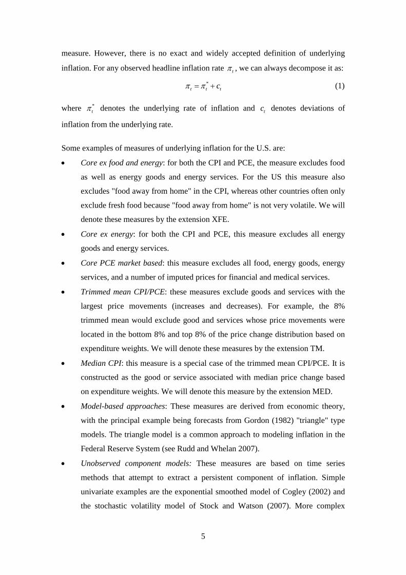
inflation. For any observed headline inflation rate tπ , we can always decompose it as:

*t t tcπ π= + (1)

where *

tπ denotes the underlying rate of inflation and tc denotes deviations of

inflation from the underlying rate.

Some examples of measures of underlying inflation for the U.S. are:

• Core ex food and energy: for both the CPI and PCE, the measure excludes food

as well as energy goods and energy services. For the US this measure also

excludes "food away from home" in the CPI, whereas other countries often only

exclude fresh food because "food away from home" is not very volatile. We will

denote these measures by the extension XFE.

• Core ex energy: for both the CPI and PCE, this measure excludes all energy

goods and energy services.

• Core PCE market based: this measure excludes all food, energy goods, energy

services, and a number of imputed prices for financial and medical services.

• Trimmed mean CPI/PCE: these measures exclude goods and services with the

largest price movements (increases and decreases). For example, the 8%

trimmed mean would exclude good and services whose price movements were

located in the bottom 8% and top 8% of the price change distribution based on

expenditure weights. We will denote these measures by the extension TM.

• Median CPI: this measure is a special case of the trimmed mean CPI/PCE. It is

constructed as the good or service associated with median price change based

on expenditure weights. We will denote this measure by the extension MED.

• Model-based approaches: These measures are derived from economic theory,

with the principal example being forecasts from Gordon (1982) "triangle" type

models. The triangle model is a common approach to modeling inflation in the

Federal Reserve System (see Rudd and Whelan 2007).

• Unobserved component models: These measures are based on time series

methods that attempt to extract a persistent component of inflation. Simple

univariate examples are the exponential smoothed model of Cogley (2002) and

the stochastic volatility model of Stock and Watson (2007). More complex

6

multivariate examples are the Chicago Fed National Activity Index for GDP and

the model for inflation used in this paper.

• Market or survey based approaches: These measures are derived from financial

markets (e.g. treasury implied securities or TIPS) or surveys of inflation

expectations (e.g. University of Michigan Consumer Inflation Expectations).

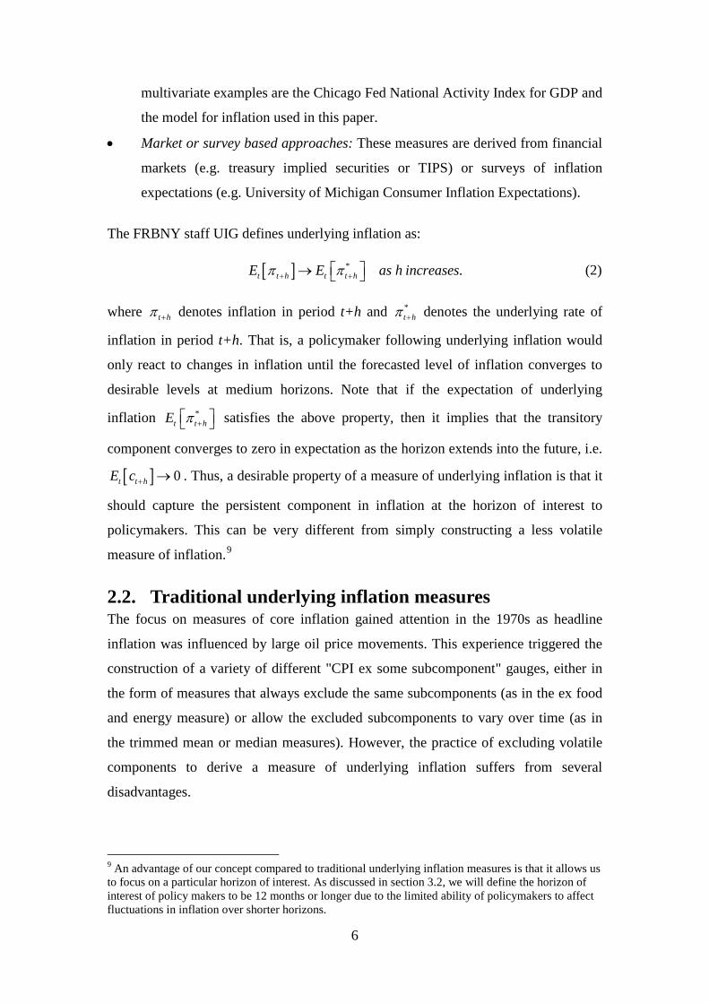
The FRBNY staff UIG defines underlying inflation as: [ ] * .t t h t t hE E as h increasesπ π+ + → (2) where t hπ + denotes inflation in period t+h and *

t hπ + denotes the underlying rate of

inflation in period t+h. That is, a policymaker following underlying inflation would

only react to changes in inflation until the forecasted level of inflation converges to

desirable levels at medium horizons. Note that if the expectation of underlying

inflation *t t hE π + satisfies the above property, then it implies that the transitory

component converges to zero in expectation as the horizon extends into the future, i.e.

[ ] 0t t hE c + → . Thus, a desirable property of a measure of underlying inflation is that it

should capture the persistent component in inflation at the horizon of interest to

policymakers. This can be very different from simply constructing a less volatile

measure of inflation.9

2.2. Traditional underlying inflation measures The focus on measures of core inflation gained attention in the 1970s as headline

inflation was influenced by large oil price movements. This experience triggered the

construction of a variety of different "CPI ex some subcomponent" gauges, either in

the form of measures that always exclude the same subcomponents (as in the ex food

and energy measure) or allow the excluded subcomponents to vary over time (as in

the trimmed mean or median measures). However, the practice of excluding volatile

components to derive a measure of underlying inflation suffers from several

disadvantages.

9 An advantage of our concept compared to traditional underlying inflation measures is that it allows us to focus on a particular horizon of interest. As discussed in section 3.2, we will define the horizon of interest of policy makers to be 12 months or longer due to the limited ability of policymakers to affect fluctuations in inflation over shorter horizons.

7

In the case of the ex food and energy measure, the specific subcomponents to be

removed are determined in a strictly backward looking manner based on the historical

behavior of the "noise" that has appeared in the inflation release. In their

comprehensive comparison of core inflation measures, Rich and Steindel’s (2007)

conclusion that no single core measure outperforms the others over different sample

periods is due to the fact that there is considerable variability in the nature and sources

of transitory price movements.

Additionally, in the case of the trimmed mean measure, the excluded subcomponents

are determined by a technical criterion. Usually the cut-off percentage (whether

symmetric or not) is fixed to the value that minimizes the errors in forecasting

underlying inflation (with the latter often defined as a centered 36-month moving

average of CPI inflation). However, by excluding components that display large price

changes (of either sign) and only including components that display more moderate

price changes, the reduced volatility may also remove any early signals of changes in

the inflation process that tend to show up in the tails of the price change distribution.

Therefore, even though the average forecast error might be low using an exclusion-

based approach, the core inflation measure might be a lagging indicator at turning

points.

Core inflation measures that exclude large price changes are subject to another

criticism. In particular, critics argue that excluding the largest price changes limits

movements in inflation by definition, and thereby narrows the range of possibly

reported outcomes. For example, many analysts argue that the sustained oil price

increase through mid-2008 should have been interpreted as a signal about the trend in

price changes and not as a series of temporary outliers. Their argument was based on

the view that oil price increases since 2000 were driven mostly by long-term supply

and demand considerations rather than short-term supply disruptions – the

traditionally cited reason to exclude oil prices. In this case, excluding the direct

effects of oil would be misleading or at least produce a lagged inflation signal. This

example demonstrates the need for underlying inflation measures to be able to smooth

short-term volatility in inflation without neglecting potentially informative price

changes.

8

2.3. Data rich models of underlying inflation Given the limitations of measures of underlying inflation that exclude volatile

variables, we look into measures based on data rich models.10

Characteristics of data rich models

One of the most prominent differences between exclusion-based measures of

underlying inflation and data rich models of underlying inflation is that the focus of

the latter is not limited to an inflation measure or its subcomponents. Simplicity is the

main advantage of the exclusion-based measure, and its performance, as shown by

Atkeson and Ohanion (2001), can be very similar or even better than more

complicated approaches. From a policy perspective as well as from a forecasting

perspective, however, there are several reasons why it is beneficial to add, rather than

exclude, information to measure underlying inflation. As argued in Bernanke and

Boivin (2003), monetary policymaking operates in a "data rich environment".

Furthermore, Stock and Watson (1999, 2008) show that a broad information set can

improve forecast accuracy in certain time periods. Therefore, several authors

(including Gali (2002)) argue that a policymaker would benefit from a comprehensive

measure that extracts and summarizes the relevant information for inflation from a

broader data set.

One popular approach that includes other variables than just inflation data is based on

Gordon (1982) and the estimation of a backward looking Phillips curve type model.

This approach considers labour market information along with price data and

additional covariates to capture exogenous pricing pressures such as those from

energy. Underlying inflation measures can then be derived by specifying the future

path of exogenous covariates and generating forecasts from the model.11 A criticism

of this particular approach is that it is very sensitive to the particular model

specification (see Stock and Watson 2008).

Factor models

Another class of data rich models are factor models, which aim to summarize the

information contained in many variables into a small number of variables – referred to 10 We refer to a ‘data rich model’ as a model that uses a broad data set that is larger than what a regression could accommodate without introducing multicollinearity and degrees of freedom issues. 11 For example, one could specify a path for energy prices based on futures market information.

9

as factors. We investigate the use of factor models, which has three main advantages:

a broad data approach, flexibility, and smoothness.

(a) broad representation of economic developments

First, factor models can be applied to a particularly broad information set and used to

summarize price pressures in a formal and systematic way. In the various exclusion-

based measures, some individual goods and service prices are omitted. Factor

techniques allow us to use all the information in the monthly US CPI inflation report.

Furthermore, there are many other time series that may be useful to measure

underlying inflation. Specifically, information about future price pressures is

incorporated in real and financial variables. For example, slack or tightness in product

and labour market are often cited as possible determinants of inflation. However, none

of this information is used to construct traditional underlying inflation measures.

(b) flexible weighting scheme

Second, standard Phillips curve models rely on one measure of slack and are

vulnerable to specification errors in this regard. The factor model approach allows

information to be extracted in a flexible manner from a very large data set. When

estimating the factors, the correlations between the variables are considered without

imposing any restriction on sign or magnitude. This differs from the strong

assumptions often made, for example, in structural VAR-models.

(c) smoothness

Third, the type of factor model used to construct the UIG – the dynamic factor model

– allows for an evaluation of whether a large movement in a particular price is likely

to persist over a specified period of time (e.g., 12 months or longer). If the price

movement is likely to persist, then it will influence the estimate of underlying

inflation. In contrast, traditional exclusion-based measures will initially ignore a large

price movement (e.g. in energy prices) and only incorporate it at a later date if and

when the price movement has passed-through to the prices of other items included in

the exclusion-based measure.

10

3. FRBNY Staff Underlying inflation gauge (UIG) The FRBNY Staff UIG examines a broad data set and uses up-to-date statistical

techniques in its derivation. In this section we describe the data set, the estimation

procedure as well as the parameterization of the model.

3.1. Data Sample range

Based on substantial evidence of structural breaks in the US inflation process (see

Clark (2004) and Stock and Watson (2008) for a comprehensive evaluation), we limit

our analysis to the period starting in January 1993. For similar reasons, the OECD

(2005) divides the sample for a multi-country study of inflation into the sub periods

1984-1995 and 1996-2004. In addition, there is a tension between our data rich

environment approach and the statistical methodology that requires a balanced data

set to start the estimation, requiring us to strike a balance between the length of the

time period of the study and the range/broadness of time series we can use. These

considerations reinforced the choice of January 1993 as the start date, as an earlier

time period would have limited significantly the number of times series that could be

considered for the analysis.

We use two data sets from the following broad categories: (i) goods and services

prices (CPI, PPI); (ii) labor market, money, producer surveys, and financial variables

(short and long term government interest rates, corporate and high yield bonds,

consumer credit volumes and real estate loans, stocks, commodity prices). We refrain

from including every available indicator that could have a possible impact on inflation

because research on factor models (see Boivin and Ng (2006)) shows this does not

come without risks.12 Our approach is to include the variables that were regularly

followed by the FRBNY staff in their assessment over several economic cycles. This

procedure has the benefit of drawing upon their long-term experience and maintains

some continuity in the set of variables on which the UIG is based. Ideally, the

variables considered to construct the UIG remain the same over several cycles, so as

to assure that a change in the UIG is not caused by changes in the data composition

through the addition or removal of series. The weighting of each series in the UIG 12 Their results suggest that factors estimated using more data do not necessarily lead to better forecasting results. The quality of the data must be taken into account, with the use of more data increasing the risk of ‘leakage of noise’ into the estimated factors.

11

changes over time and is determined by the factor model. Figures 1a and 1b provide

more information on the current data set used, while the Data Appendix provides a

detailed listing of the variables.

Stability of UIG when data are revised

In order to derive a signal of underlying inflation for monetary policymakers, stability

of the most current estimates becomes an important issue. Therefore, nearly all of the

data selected is not subject to revision. This implies that we must rely heavily on

survey data for measures of real activity and not use more traditional measures based

on the National Income and Product Accounts. Another advantage of survey data is

that it is usually released more quickly than expenditure and production data.

Additionally, we only use non-seasonally adjusted data and, following Amstad and

Fischer (2009a and b), apply filters within the estimation procedure to generate a

seasonally adjusted estimate of underlying inflation. The main reason for adopting

this approach is that it prevents revisions in our measure of underlying inflation from

being driven by concurrent seasonal adjustment procedures.

As is standard in the factor model literature, prior to estimation the data is

transformed to induce stationarity and each series is standardized so that it has zero

mean and unit variance. The standardization process requires us to assign an average

value for the measures of underlying inflation derived from the analysis. We use

2.25% for the CPI and 1.75% for the PCE. When we began the project at the end of

2004, these numbers were very close to the respective average inflation rates starting

from 1993.13

13 A growing number of countries establish their monetary policy more or less explicitly according to an inflation target. In these countries the information on the inflation targeting regime is useful for constructing the measure of underlying inflation. In particular, if the country has a point target, then the average of the underlying measure should be at this point target. A feature of the dynamic factor model technique we use is that it does not directly provide an estimate of the average of the underlying measure. Thus, in countries with inflation targets the target can be used as the average. When we started this analysis, the Federal Reserve had not stated a numerical inflation goal. In January 2012, the FOMC agreed to a longer-run goal of a 2 percent PCE inflation rate. This is higher than the value we have assumed for PCE inflation but, according to some estimates, is close to our assumption for CPI inflation.

12

Real-time updates

The UIG is designed as a model of monthly inflation that is updated daily as

suggested by Amstad and Fischer (2004, 2009) in their work using Swiss data. The

monthly dating of the UIG is motivated by the monthly frequency of inflation reports

in the U.S. The daily updates allow for a close monitoring of the inflation process and

also provide a basis for monetary policymakers to assess movements in underlying

inflation due to daily changes in financial markets between monthly inflation reports.

3.2. Estimation procedure We follow the dynamic factor model approach of Forni, Hallin Lippi and Reichlin

(2000), which draws upon the work of Brillinger (1981) and extends it for use with

large data sets. An econometric summary of the procedure is given in the Technical

Appendix of Amstad and Potter (2009). In this section, we motivate the choice of

important parameters of the model.14 In particular, we discuss the time horizon of

interest for the UIG, as well as the number of factors used to summarize the

information content of the whole data set.

Horizons of interest

We want the UIG to be useful for monetary policymakers and long-term investors.

Lags in the monetary transmission mechanism suggest that inflation at a horizon of

one year or less is relatively insensitive to changes in current monetary policy, and

therefore there is little that policymakers can do to affect these fluctuations in

inflation. Consequently, if monetary policy has been achieving its objective of price

stability with well anchored inflation expectations, then the effects of current

movements in monetary policy on expected inflation will be at horizons greater than

12 months. Thus, we focus on horizons of 12 months and longer to extract the

factors.15

14 Please note that the approach in this paper allows us to set these parameters exogenously. For FRBNY internal analysis different parameter settings are evaluated on a regular basis (e.g., different time horizons). 15 In practice, the estimation is done directly in the frequency domain, as described in the Technical Appendix of Amstad and Potter (2009)

13

Number of factors

Different papers find that much of the variance in U.S. macroeconomic variables is

explained by two factors. Giannone, Reichlin and Sala (2005) show this result using

hundreds of variables for the period 1970-2003, as well as Sims and Sargent (1977)

who examine a relatively small set of variables and use frequency domain factor

analysis for the period 1950-1970. Watson (2004) notes that the two-factor model

provides a good fit to U.S. data during the post-war period, and that this finding is

quite robust. Hence, in most large data factor model applications the number of

factors is set to two.

The factors in a data set can be interpreted as ‘drivers’ of the data set. It is often

claimed that one factor is associated with real variables (such as GDP or aggregate

demand), while the second factor is associated with nominal prices (such as the CPI).

Our choice of the number of factors is not based on this consideration. Rather, our

aim is to include the lowest number of factors needed to represent our data

environment properly, without any attempt to label the factors (as either real or

nominal) or to interpret them.

We start our examination of the UIG measure by presenting estimates based only on

price data from the CPI and PCE, respectively.16 One would expect these series to be

driven by one single factor. Figures 2a and 2b show, respectively, the estimates for

the UIG for CPI inflation and PCE inflation assuming 1 and 2 factors along with the

12 month change in the relevant price index. As shown, there is little difference

between the two estimates. Further, the movements in the estimates are generally very

smooth when we only consider frequencies of 12 months or longer, with the exception

of those observed during the 2008-2011 period.17

16 We refer to these as CPI_UIG_Prices Only and PCE_UIG_Prices Only, while CPI_UIG and PCE_UIG will refer to the UIG measures derived from using all the variables shown in Data Appendix. 17 We investigated the issue of smoothness during our initial work in the initial construction of the UIG in 2005 through the following experiment: take a monthly CPI release and scale up all of the 211 time series by a fixed amount. The result of the experiment was a big upward movement in the UIG indicating that the method could capture a common movement in all of the individual price series. Later, during the financial crisis in 2008/09, the smoothness of the UIG was revisited through a real world example. Again, as will be further illustrated in section 4, the UIG displayed a big change that reflected the large movements in the underlying data. It should be noted that if we were to include all frequencies in the estimation of the UIG, then as would be expected there would be a very close correspondence between the movements in total inflation and the UIG.

14

Figures 3a and 3b show the estimated UIG for a range of 1 through 8 total factors,

where we now add the non-price variables in our dataset through July 2012. Three

findings are noteworthy. First, the estimates now show larger cyclical fluctuations.

Second, starting in 2005 they correctly capture a broadly downward sloping trend

despite the temporary large increase in inflation in the first half of 2008. Third, there

is usually little difference between the estimates based on 2 or more factors, with the

exception of two episodes that occurred during the mid-1990s and from 2008 through

the end of 2011.

4. Comparing measures of underlying inflation This section compares well-known traditional underlying inflation measures (core

inflation measures) and the UIG measure for CPI and PCE inflation. First we

comment on general statistical differences. Next we turn to the time series features of

the various underlying inflation measures and compare their ability to track as well as

to forecast inflation.

4.1. General statistical properties We find that the general behaviour of the different measures of underlying inflation is

mainly driven by the choice of methodology (see section 2) and less by the choice of

the price index. This is illustrated by the time series plots in Figures 4a-c that depict

the same underlying inflation measure for different price indices. In Figures 5a and 5b

we show the various underlying inflation measures for each price index. We now

comment on three main statistical features of the underlying inflation measures:

smoothness, correlation with headline CPI inflation and headline PCE inflation, and

the correlation between the UIG for CPI inflation and the UIG for PCE inflation.

First, based on standard deviation metrics (see Table 1), the UIG (augmented by the

non-price variables) is less volatile than CPI / PCE inflation but more volatile than the

traditional underlying inflation measures. However, standard deviation metrics

consider volatility across all frequencies, from high to low. Figures 4a–c show that the

UIG displays the lowest short run volatility – that is, the UIG provides the smoothest

signal at high frequencies. This should not be surprising because the UIG focuses on

cycles of 12 months or longer. Thus, the ex-food and energy measure and, to a lesser

extent, the trimmed mean provide a signal that retains some high frequency volatility,

15

which then makes it more difficult for a policymaker to determine if a change in core

inflation measures merit a policy action.

Second, the UIG closely tracks headline CPI/PCE inflation and at the same time is

able to provide additional information to the policymaker that is not included in

traditional underlying inflation measures. Compared to popular core inflation

measures, the UIG displays the highest correlation with CPI inflation and PCE

inflation respectively (see Tables 2a and 2b). Meanwhile, the UIG is less correlated

with traditional underlying inflation measures, although this finding holds more for

the CPI than PCE. However, in both cases it is evident that the UIG is providing a

different signal than the traditional underlying inflation measures. This conclusion is

confirmed by a simple principal components analysis (PCA) on the CPI and

underlying inflation measures that include the UIG.18 As shown by the factor

loadings given in Table 3, the traditional underlying inflation measures are grouped in

the first principal component, while the UIG and CPI inflation are grouped in the

second principal component.

Third, although there are clear differences between the UIG for CPI inflation and the

UIG for PCE inflation, they are highly correlated with each other as can be seen in

Table 2c. This is also true if we restrict the data set for extracting factors to prices

only. Going forward, we will focus more on the CPI-based UIG to save space and

because it has the advantage that the CPI is only subject to very minor and rare

revisions whereas the PCE is subject to major revisions especially in the non-market

based prices.19

4.2. Forecast Performance A central reason for developing underlying measures of inflation is that they should

produce more accurate forecasts of inflation than those generated using only the

headline measure. For any evaluation, it is particularly important that the forecast

18 Principal component analysis arranges variables in groups (referred to as principal components) based on their statistical behaviour. This is done in a way to assure by construction that variables with similar behaviour are grouped in the same principal component, with each of the principal components uncorrelated with each other. 19 However, both underlying inflations gauge for CPI (CPI_UIG) and for PCE (PCE_UIG) are calculated by the FRBNY internally.

16

exercise reflects a realistic setting. Following Cogley (2002) and others, we initially

evaluate the within-sample performance of the various measures of underlying

inflation by estimating the following regression equation for horizon h:

( )t h t h h t mt t hπ π α β π π µ+ +− = + − + (3)

where mtπ denotes the relevant measure of underlying inflation. Two desirable

properties of an underlying measure of inflation are unbiasedness

( )0 1h handα β= = − and the capability to explain a substantial amount of the future

variation in inflation. If hβ were negative but less than one in absolute value, then the

deviation between headline inflation and the underlying inflation measure ( )t mtπ π−

would overstate the magnitude of subsequent changes in inflation, and thus would

also overstate the magnitude of the current transitory deviation in inflation. Similarly,

if hβ were negative but greater than one in absolute value, then the deviation between

headline inflation and the underlying inflation measure would understate the

magnitude of the current transitory deviation in inflation. This specification also nests

the random walk model of Atkeson and Ohanion (2001) when 0.h hα β= =

When equation (3) is estimated within sample, our main interest is testing for

unbiasedness and whether the transitory deviation in inflation displays the correct size

( )1hβ = − . Using a long sample period and examining traditional underlying inflation

measures, Rich and Steindel (2007) find that the property of unbiasedness can be

rejected, but there is less evidence against the hypothesis that the coefficient on the

deviation equals -1. In our shorter sample, we are unable to reject either hypothesis.

However, it should be noted that the test for unbiasedness of the UIG suffers from

pre-test bias as the UIG must be centered separately from the estimation of the

factors20. Further, while it is always possible to reject the model of Atkeson and

Ohanion based on within sample estimation, this is not informative about a model’s

out of sample performance, which we address in the following section.

20 As mentioned in section 3.1 and in footnote 13, the standardization of the variables requires us to assign an average value for the underlying inflation gauges for CPI inflation and PCE inflation.

17

Note of caution for forecasting exercises

We now investigate the relative performance of underlying inflation measures through

their ability to forecast inflation in real-time. It is often argued that a forecasting

exercise will be able to identify the best underlying inflation measure. However, there

are several aspects of these types of comparisons that require care, particularly when

it comes to producing underlying measures of inflation for use by policymakers.

Therefore we want to add some preliminary remarks and use them as a note of caution

before we undertake the usual forecasting exercise in the broadly accepted setting of

Rich and Steindel (2007).

The most difficult aspect – which should be considered in the interpretation of

forecasting results – is the appropriate loss function to measure forecast accuracy. The

standard approach is to use a quadratic loss function for the forecast errors. Consider

the following example:

• case 1: For total inflation between 1% and 3% the RMSE at 12 months for

underlying measure A is 1 percentage point, while for measure B it is 1.1

percentage points.

• case 2: For total inflation outside of 1% and 3% the RMSE at 12 months for

underlying measure A is 2 percentage points, while for measure B it is 1.2

percentage points.

If the policymaker uses measure A, then they will be slower to recognize a change in

the trend in underlying inflation compared to using measure B. Suppose the

policymaker successfully uses measure B to conduct monetary policy so that total

inflation is rarely outside of a range of 1-3%, then a forecast evaluation would favour

measure A if actual inflation was outside the 1-3% range less than 10 percent of the

time. Therefore, forecast accuracy may not be informative about the usefulness of an

underlying inflation measure for stabilization purposes.

Besides recognizing that the results may need to be interpreted with some caution,

another important issue for the exercise concerns the choice of the forecasting sample

period. Long time periods can be problematic because they might cover different

18

inflation regimes. Furthermore, because most industrialized countries successfully

stabilised their inflation rates before the financial crisis, the signal associated with the

least variation (e.g. a constant) might have had an advantage compared to signals

generated from earlier periods when there were more fluctuation in inflation. The

opposite result might hold for measures with more variability during the financial

crisis. Therefore it is important to run the exercise over a sample displaying

significant variation in inflation as well as over different sub-samples. The behaviour

of inflation in the US since 2000 displays these features as it is relative tranquil during

the pre-2008 period, but extremely volatile during the post-2008 period.

Finally, forecasting exercises are often undertaken in a "pseudo" real-time manner in

which estimation is conducted using a single vintage data set. In practice, the actual

data used might have been revised subsequently. In our case, the UIG is constructed

from data that is either not revised or only revised slightly (some PPI prices) but,

unlike more traditional exclusion-based measures, future data can lead to

reassessments of its previous values. Consequently, we will focus on the CPI because

its revisions are very minor (correction of small technical mistakes) and thus the

forecast target and the underlying measures used for comparison can be treated as if

they are real-time data.21

A“horse race”: UIG versus traditional underlying inflation measures (‘core

measures’)

We first consider the results of a forecasting exercise based on an estimated version of

equation (3):22

( )ˆˆˆt h t h h t mtπ π α β π π+ = + + − (4)

where , ,ˆˆ ,h t h tα β are the estimated regression coefficients using data through time t.

Estimation starts in 1994, while the forecasting range spans the period from 2000

through the middle of 2012. To account for possible sensitivity of the forecast

21 Because we focus on the 12 month horizon there is no meaningful difference between seasonally adjusted and non-seasonally adjusted measures. 22 To ensure comparability we use the same setting as in the paper of Rich and Steindel (2007), which compares forecast performance of traditional core measures. The same regression model has been used in studies such as Clark (2001), Hogan, Johnson and Laflèche (2001), Cutler (2001) and Cogley (2002).

19

comparisons to the selected sample periods, we consider two different sub-sample

periods. First, a pre-crisis sub-sample from 2000-2007, a time range that could be

considered a representative inflation cycle as it encompasses moderate cyclical phases

in CPI inflation. Second, a crisis sub-sample that captures the period from 2008 until

the middle of 2012. Finally, for comparison purposes we also consider a sample from

2001 to 2007 that exactly matches one considered in Stock and Watson (2008). We

compare the forecast performance of the UIG to the ex-food and energy, trimmed

mean, and median measures. We also include a prices only version of the UIG as well

as the prior 12 month change in CPI inflation in the forecast exercise.

The results in Table 4 show that the UIG clearly outperforms the traditional

underlying inflation measures in forecasting headline CPI before the crisis, during the

crisis, as well as over the whole sample range. This is evident from the lowest

reported RMSE over all samples. To analyse the UIG forecast performance further,

we apply the Diebold-Mariano (1995) testing procedure23. The results show that the

forecast errors from the UIG are lower than those from the traditional underlying

inflation measures at a 5% statistical significance level during the crisis, and mostly at

a 1% statistical significance level before the crisis as well as over the whole sample.

When we focus solely on the traditional underlying inflation measures, they do not

differ much in their forecasting performance, confirming the previous findings in Rich

and Steindel (2007). However, there are three notable observations for the traditional

underlying inflation measures. First, all underlying inflation measures do better than

the 12 month change in total CPI inflation – the random walk forecast – which, not

surprisingly, displays the highest forecast errors among the reported measures and

samples during the crisis.24 Secondly, the forecasting performance of the CPI trimmed

mean and CPI median are remarkably similar over all samples. Third, the forecasting

performance of the popular CPI ex-food and energy measure relative to the other

measures is better during the crisis than before the crisis25.

23 Diebold and Mariano (1995) propose and evaluate explicit tests of the null hypothesis of no difference in the forecast accuracy of two competing models. 24 The forecast from the random walk model is the current value of the variable, which would be expected to perform poorly during episodes when inflation is particularly volatile. 25 Before the crisis, the CPI ex-food and energy measure displayed the poorest forecast performance of the reported measures. During the crisis, the CPI ex-food and energy measure generated lower forecast errors than the CPI trimmed mean and the CPI median.

20

An important consideration in evaluating the results in Table 4 is that the UIG has the

advantage of being derived from a process that uses information from revised values

of the non-price components in the dataset. One approach to assess the significance of

this advantage is to re-estimate the UIG at each time period. However, such a

procedure would not be necessary if the revisions to past UIG estimates were small as

new data was added. We examine this issue in the next section.

UIG revisions historically and during the crisis period

The UIG is constructed using the most current information, with revisions to the UIG

resulting either from new observations of the input variables or from revisions to

previous values of the input variables. Revisions of an underlying inflation gauge can

be judged as either helpful or uninformative. An ideal measure should show only

modest revisions during normal economic times. On the other hand, such a measure is

expected to be highly responsive to changes in a volatile economy and to reflect this

through revisions that readily incorporate new information in the course of providing

updates of the past.

To examine whether the UIG behaves in a manner similar to that of the ideal measure

described above, we examine a 26-month period before the crisis from November

2005 to December 2007 and a 44-month period during the crisis from January 2008 to

August 2011. The first phase covers a time period with economic changes that were

very typical when judged on an historical basis, while the second phase covers a time

period of historically large economic changes. Given the events in the current crisis,

we think of the second sub-sample as a real world stress test that provides an

assessment of the maximal revision that can occur to the UIG.

We examined the daily revisions to each of the estimates of the monthly UIG

estimates over 240 workdays (approximately one year). The results of this exercise

are presented in Figures 6a and 6b for the absolute size of the change, where we plot

the mean and median of the change of the UIG estimate from the x-th workday

compared with the final estimate. We examine the absolute values to ensure that large

changes in one direction are not cancelled out by large changes in the opposite

direction. As shown, during a normal business cycle (November 2005 to December

2007) the largest changes in the estimate of the UIG for a month usually occur within

21

the first month (20 workdays). The maximal median and mean revision in UIG

amounts to a change of about 8 and 14 basis points, respectively (Figure 6.a). The

source of these changes is the publication of the monthly CPI report. After that the

mean and median revisions converge to zero.26 Since 2008, with the large decline in

CPI inflation and the deep recession in the US, the revisions in the input variables and

therefore also the UIG have been considerably larger. During this period of extremely

volatile news flows, the maximal mean and median revision in UIG amounted to 80

and 60 basis points, respectively (Figure 6.b).

The preceding evidence suggests two findings. First, the UIG appears to display the

desired behaviour of an ideal measure of underlying inflation in that it remains very

stable during normal economic times, but is able to adapt quickly in turbulent times.

Second, given the fast convergence of the revisions to zero, particularly after the first

month, and because the forecasting exercise uses only monthly data over several

years, we consider the impact of the revisions on the forecasting performance of the

UIG as limited.

A real-time out of sample forecast comparison

After observing that the UIG displays greater accuracy in a pseudo out-of-sample-

forecasting exercise and documenting the limited impact on its performance from

revisions, we now conduct a real-time out-of-sample forecasting comparison. Real-

time forecasts from the UIG have been produced each day starting in November 2005.

These forecasts are produced directly from the statistical factor model underpinning

the UIG rather than from prediction models based on equation (3). The original

motivation for the daily real-time updates was to compare any changes in these

forecasts with movements in inflation expectations from financial markets, which are

also available daily. The real-time forecasts were produced for a range of horizons (1,

2-3 and 3-5 years). The real-time out-of-sample forecasts at the one year horizon were

also used for comparisons to forecasts based on the prior 12 month change in the CPI

and core CPI. The target variables were both the CPI and the core CPI. The results are

presented in Table 5 for the sample period from November 2006 to April 2009. Using

26 The finding that the mean converges more slowly to zero than the median likely reflects the sustained period of CPI inflation over 3% in the evaluation period - an ex ante unlikely event given our decision to center the UIG at 2.25% and the volatility of the CPI from 1993-2005.

22

a real-time out-of sample exercise, we again find the UIG outperforms the traditional

underlying inflation measures.

CPI and the labour market as drivers of UIG

Finally, we examine in more detail the changes in the estimated path of the UIG since

1995 using data through the last two months of 2008 and the first month of 2009. For

each month we show the path of the UIG after the release of the CPI in the prior

month (i.e., the CPI for two months earlier), the release of the U.S. employment

situation for the prior month, and finally the release of the CPI for the prior month.

The results are presented in Figures 7.a through 7.c. The results for November

indicate little response to the CPI or the employment situation for October 2008. In

December 2008 it can be seen that the November CPI had a large effect on the current

value of the UIG and the estimates for the previous 24 months. Finally, the December

2008 employment situation produced a large change in the current estimate (i.e.,

January 2009) of the UIG and significantly altered its whole history.

5. Conclusions This paper presents some background and properties on the FRBNY staff underlying

inflation gauge. UIG adds to the existing literature on U.S. inflation and complements

the standard measures of core and underlying inflation available to monetary

policymakers and long-term investors in the following ways.

First, UIG summarises in a single number the information content in a broad data set

including asset prices and real variables like unemployment rate. Unlike traditional

core measures UIG does not restrict itself to price data in one point of time only, as

many economic variables may affect the inflation process and may do so in a time

varying manner. The carefully chosen data set reflects the information which is

considered as informative to forecast inflation by FRBNY staff economists.

Second, similar to inflation expectation derived from financial markets, UIG can be

evaluated daily and considers changing correlations in the data set.

23

Third, UIG is able to measure underlying inflation at a frequency of relevance to

policymakers and long-term investors. The smooth cyclical patterns of UIG give

policymakers and market participants a clear indication of which CPI movements and

developments are likely to be persistent and therefore could require a response from

monetary policy.

Fourth, while UIG is closely related to headline inflation, it at the same time adds

important additional information on underlying inflation over that contained in

traditional core measures. Therefore UIG can be used in addition to other core

measures more mainly in a complementary than a substitutive way.

Finally, in a competitive horse race setting of forecasting head line inflation UIG

significantly outperforms traditional core measures for different regimes of headline

inflation. These findings hold for a sample from 2000 to mid of 2012 as well as for a

sample focusing on an average economic regime before the crisis as well as an

extremely volatile sample during the crisis.

These features make UIG particularly useful for policy makers and market

participants.

24

References

Alesina, Alberto, Olivier Blanchard, Jordi Gali, Francesco Giavazzi and Harald Uhlig (2001), ‘Defining a Macroeconomic Framework for the Euro Area - Monitoring the European Central Bank, 3, CEPR 2001.

Altissimo, F.,A. Bassanetti, R. Cristadoro, M. Forni, M. Hallin, M. Lippi, L.Reichlin, and G. Veronese (2001), ‘EuroCOIN: A Real Time Coincident Indicator for the Euro Area Business Cycle’, CEPR discussion paper No. 3108.

Altissimo, Filippo, Benoit Mojon, and Paolo Zaffaroni (2009), ‘Can Aggregation Explain the Persistence of Inflation?’, Journal of Monetary Economics, 56(2): 231–41.

Amstad, Marlene and Andreas M. Fischer (2004), ‘Sequential Information Flow and Real-Time Diagnosis of Swiss Inflation: Intra-Monthly DCF Estimates for a Low-Inflation Environment’, CEPR Discussion Papers 4627.

Amstad, Marlene and Simon Potter (2009), ‘Real-time Underlying inflation gauge for Monetary Policy Makers’, FRBNY Staff Report, No 420.

Amstad, Marlene and Andreas M. Fischer (2009a), ‘Are Weekly Inflation Forecasts Informative?’, Oxford Bulletin of Economics and Statistics, April 2009a,71(2), pp. 236-52

Amstad, Marlene and Andreas M. Fischer (2009b), ‘Do Macroeconomic Announcements Move Inflation Forecasts?’, Review Federal Reserve Bank of St. Louis, pp. 507-518, September.

Amstad, Marlene and Andreas M. Fischer (2010), ‘Monthly pass-through ratios’, Journal of Economic Dynamics and Control, Elsevier, vol. 34(7), pp. 1202-1213, July.

Ang, Andrew, Geert Bekaert and Min Wei (2007), ‘Do macro variables, asset markets, or surveys forecast inflation better?’, Journal of Monetary Economics, Elsevier, vol. 54(4), pp. 1163-1212, May.

Aron, J. and J. Muellbauer (2013), ‘New Methods for Forecasting Inflation, Applied to the US’, Oxford Bulletin of Economics and Statistics, Department of Economics, University of Oxford, vol. 75(5), pp. 637-661, October

Atkeson, Andrew and Lee E. Ohanian. (2001), ‘Are Phillips Curves Useful for Forecasting Inflation?’ Federal Reserve Bank of Minneapolis Quarterly Review, 25:1, 2–11.

Balke, N. S. and M.A. Wynne (2000), ‘An equilibrium analysis of relative price changes and aggregate inflation’, Journal of Monetary Economics, Elsevier, vol. 45(2), pp. 269-292, April.

Bernanke, B.S. and Boivin, J. (2003) `Monetary policy in a data rich environment', Journal of Monetary Economics vol. 50(3), pp. 525-546, February.

Bowley, A. L. (1928), 'Notes on index numbers', Economic Journal, 38, 216-137.

Brillinger, D.R. (1981), 'Time Series: Data Analysis and Theory', Holden-Day, San Francisco

25

Bryan, Michael F., and Christopher J. Pike (1991), ‘Median price changes: an alternative approach to measuring current monetary inflation’, Federal Reserve Bank of Cleveland Economic Commentary, December 1.

Bryan, Michael F. and Stephen G. Cecchetti (1994), ‘Measuring Core Inflation’ in: N.G. Mankiw, Monetary Policy, pp. 195-215, Chicago: University of Chicago Press.

Bryan, Michael F. and Stephen G. Cecchetti (1999), ‘Inflation And The Distribution Of Price Changes’, The Review of Economics and Statistics, MIT Press, vol. 81(2), pp. 188-196, May.

Bryan, Michael F., Stephen G. Cecchetti and Rodney L. Wiggins (1997) `Efficient Inflation Estimation', NBER Working Paper Nr. 6183.

Boivin, Jean and Serena Ng (2006), ‘Are more data always better for factor analysis?’, Journal of Econometrics, Elsevier, vol. 132(1), pp. 169-194, May.

Castelnuovo, Efrem, Sergio Nicoletti-Altimari and Diego Rodriguez-Palenzuela (2003), ‘Definition of price stability, range and point inflation targets: the anchoring of long-term inflation expectations’, ECB working paper No. 273.

Cecchetti, Stephen G. (1995), ‘Inflation Indicators and Inflation Policy’, NBER Chapters, in: NBER Macroeconomics Annual 1995, Volume 10, pages 189-236 National Bureau of Economic Research, Inc.

Cecchetti, Stephen G.(1997), 'Measuring Short-Run Inflation for Central Bankers' Review, Federal Reserve Bank of St. Louis.

Clark, Todd E. (2001), 'Comparing Measures of Core Inflation', Federal Reserve Bank of Kansas City Economic Review, v. 86, No.2, pp.5-31.

Clark, Todd E. (2004), 'An Evaluation of the Decline in Goods Inflation', Federal Reserve Bank of Kansas City Economic Review, Economic Review.

Cogley, Timothy E. (2002), 'A Simple Adaptive Measure of Core Inflation', Journal of Money, Credit and Banking, Vol. 34. No.1 , pp. 94-113, February.

Crone, Theodor M., N. Neil K. Khettry, Loretta J. Mester and Jason A. Novak (2011),.’Core measures of inflation as predictors of total inflation’, Working Paper 11-24, Federal Reserve Bank of Philadelphia.

Cutler, Joanne (2001), 'Core inflation in the U.K.', Bank of England, External MPC Unit Discussion Paper No.3, March.

Cristadoro, R., M. Forni, L. Reichlin, and G. Veronese (2001), ‘A Core Inflation Index for the Euro Area’, CEPR Discussion Paper No. 3097.

Dolmas, Jim (2005), 'Trimmed Mean PCE Inflation', Federal Reserve Bank of Dallas, Working Paper 0506.

Forni, M., M. Hallin, M. Lippi and L. Reichlin (2000), ‘The Generalized Dynamic-Factor Model: Identification And Estimation’, The Review of Economics and Statistics, vol. 82(4), pp. 540-554, November.

Forni, M., M. Hallin, M. Lippi and L. Reichlin (2005). ‘The Generalized Dynamic Factor Model: One-Sided Estimation and Forecasting’, Journal of the American Statistical Association, vol. 100, pp. 830-840, September.

Gali, Jordi (2002), 'New Perspectives on Monetary Policy, Inflation and the Business Cycle', CEPR Discussion Paper No. 3210.

26

Gavin, William T. and Kevin L. Kliesen (2008). ‘Forecasting inflation and output: comparing data-rich models with simple rules’, Review, Federal Reserve Bank of St. Louis, issue May, pp. 175-192.

Giannone, D., L. Reichlin, and L. Sala (2005), ‘Monetary Policy in Real Time’, NBER Chapters, in: NBER Macroeconomics Annual 2004, Volume 19, pp. 161-224.

Giannone, D. and T. D. Matheson (2007), ‘A New Core Inflation Indicator for New Zealand’, International Journal of Central Banking, vol. 3(4), pp. 145-180, December.

Gordon, R.J. (1982), 'Price inertia and policy ineffectiveness in the United States, 1890-1980, Journal of Political Economy, 90, (6), December, pp.1087-1117.

Hobijn, B., S. Eusepi and A. Tambalotti (2010), ‘The housing drag on core inflation’, FRBSF Economic Letter, Federal Reserve Bank of San Francisco, issue April.

Hogan, Seamus, Marianne Johnson and Thérèse Laflèche (2001), 'Core Inflation', Technical Report 89, January, Bank of Canada.

Khan, Mikael, Louis Morel and Patrick Sabourin (2013), ‘The Common Component of CPI: An Alternative Measure of Underlying Inflation for Canada’, Bank of Canada Working Paper 2013-35.

Liu Z. and G. Rudebusch (2010), ‘Inflation: mind the gap’, FRBSF Economic Letter, Federal Reserve Bank of San Francisco, issue January.

Meyer, B., G. Venkatu and S. Zaman (2013), ‘Forecasting inflation? Target the middle’, Economic Commentary, Federal Reserve Bank of Cleveland, issue April.

Mishkin, Frederic S. and Klaus Schmidt-Hebbel (2001), ‘One Decade of Inflation Targeting in the World: What Do We Know and What Do We Need to Know?', NBER Working Paper No. W8397.

OECD(2005), Economic Outlook. Volume 2005 Issue 1, ‘Measuring and assessing underlying inflation’.

Quah, Danny and Shaun P. Vahey (1995), `Measuring Core Inflation', Economic Journal, vol. 105(432), pp. 1130-1144, September.

Peach R., R. Rich and A. Cororaton (2011), ‘How does slack influence inflation?”, Current Issues in Economics and Finance, Federal Reserve Bank of New York, vol. 17 (June).Rich, Robert, and Charles Steindel (2007), ‘A comparison of measures of core inflation’, Economic Policy Review, Federal Reserve Bank of New York, issue December, pp. 19-38.

Reis, Ricardo and Mark W. Watson (2010),’Relative Goods' Prices, Pure Inflation, and the Phillips Correlation’, American Economic Journal: Macroeconomics, American Economic Association, vol. 2(3), pages 128-57, July.

Rudd, Jeremy and Karl Whelan (2007), 'Modelling inflation dynamics: a critical review of recent research', Journal of Money, Credit and Banking, vol. 39(s1), pp. 155-170.

Sargent and Sims (1977), `Business Cycle Modeling Without Pretending to Have Too Much a Priori Economic Theory,' in: New Methods in Business Cycle Research: Proceedings From a Conference, Federal Reserve Bank of Minneapolis, October, 1977, pp. 45-109.

27

Stock, J.H. and M.W. Watson (1999),Forecasting Inflation', Journal of Monetary Economics, Elsevier, vol. 44(2), pp. 293-335, October.

Stock, J.H. and M.W. Watson (2002a), `Macroeconomic Forecasting Using Diffusion Indexes', Journal of Business and Economic Statistics vol. 20(2), pp. 147-162.

Stock, J.H. and M.W. Watson (2002b), `Forecasting using principal components from a large number of predictors', Journal of the American Statistical Association, vol. 97, pp. 1167-1179.

Stock, J.H. and M.W. Watson (2007), ‘Why Has U.S. Inflation Become Harder to Forecast?’, Journal of Money, Credit and Banking, Blackwell Publishing, vol. 39(1), pp. 3-33, 02.

Stock, J.H. and M.W. Watson (2008), ‘Phillips Curve Inflation Forecasts’, NBER Working Papers 14322.

Stock, J.H. and M.W. Watson (2010), ‘Modeling Inflation After the Crisis’, NBER Working Papers 16488, National Bureau of Economic Research, Inc.

Vega, J. L. and M.A. Wynne (2001), ‘An evaluation of some measures of core inflation for the euro area’, Working Paper Series 0053, European Central Bank.

Vining, Daniel R., Jr., and Thomas C. Elwertowski (1976), 'The relationship between relative prices and the general price level', American Economic Review, 66(4), pp. 699-708, September.

Watson (2004), `Comment on Giannone, Reichlin and Sala's 'Monetary Policy in Real-time', June 2004.

Wynne, M.A. (2008), ‘Core inflation: a review of some conceptual issues’, Review, Federal Reserve Bank of St. Louis, issue May, pp. 205-228.

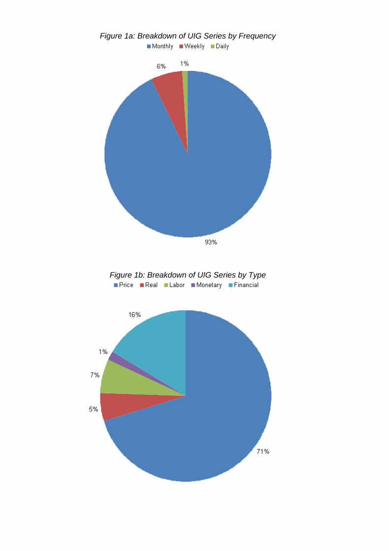
Figure 1a: Breakdown of UIG Series by Frequency

Figure 1b: Breakdown of UIG Series by Type

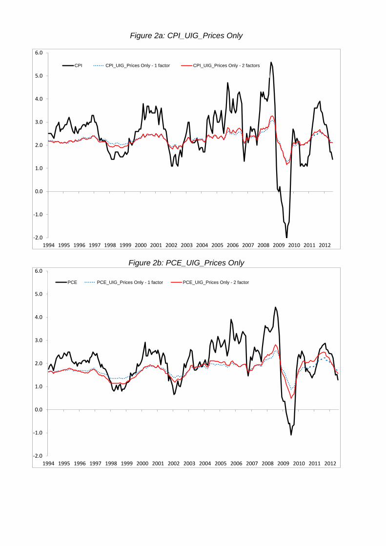
Figure 2a: CPI_UIG_Prices Only

-2.0

-1.0

0.0

1.0

2.0

3.0

4.0

5.0

6.0

1994 1995 1996 1997 1998 1999 2000 2001 2002 2003 2004 2005 2006 2007 2008 2009 2010 2011 2012

CPI CPI_UIG_Prices Only - 1 factor CPI_UIG_Prices Only - 2 factors

Figure 2b: PCE_UIG_Prices Only

-2.0

-1.0

0.0

1.0

2.0

3.0

4.0

5.0

6.0

1994 1995 1996 1997 1998 1999 2000 2001 2002 2003 2004 2005 2006 2007 2008 2009 2010 2011 2012

PCE PCE_UIG_Prices Only - 1 factor PCE_UIG_Prices Only - 2 factor

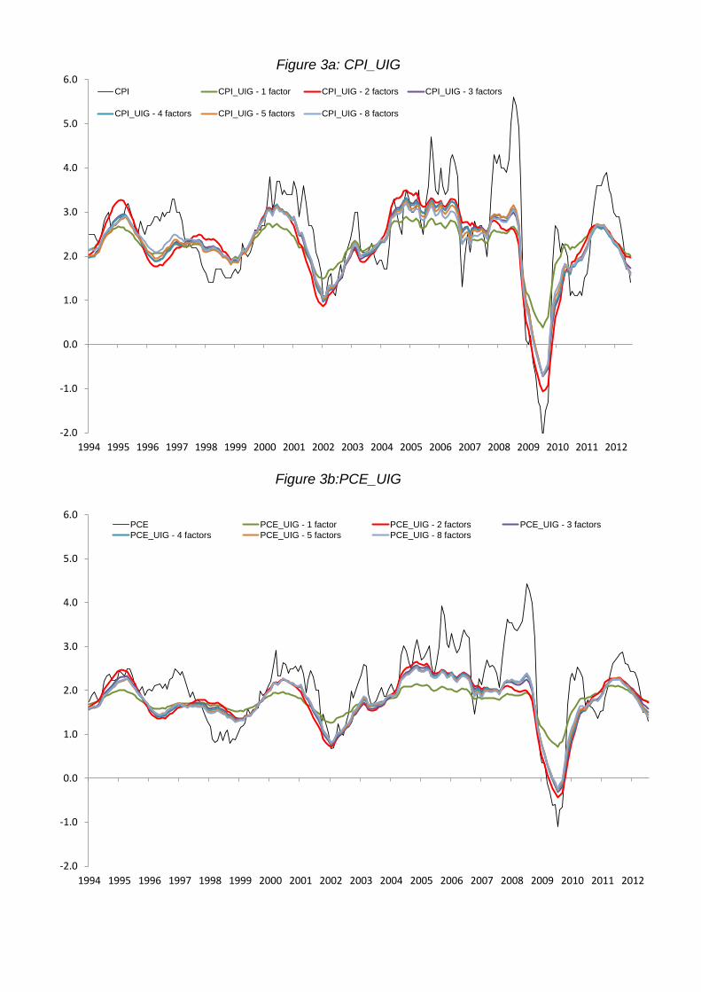
Figure 3a: CPI_UIG

-2.0

-1.0

0.0

1.0

2.0

3.0

4.0

5.0

6.0

1994 1995 1996 1997 1998 1999 2000 2001 2002 2003 2004 2005 2006 2007 2008 2009 2010 2011 2012

CPI CPI_UIG - 1 factor CPI_UIG - 2 factors CPI_UIG - 3 factors

CPI_UIG - 4 factors CPI_UIG - 5 factors CPI_UIG - 8 factors

Figure 3b:PCE_UIG

-2.0

-1.0

0.0

1.0

2.0

3.0

4.0

5.0

6.0

1994 1995 1996 1997 1998 1999 2000 2001 2002 2003 2004 2005 2006 2007 2008 2009 2010 2011 2012

PCE PCE_UIG - 1 factor PCE_UIG - 2 factors PCE_UIG - 3 factorsPCE_UIG - 4 factors PCE_UIG - 5 factors PCE_UIG - 8 factors

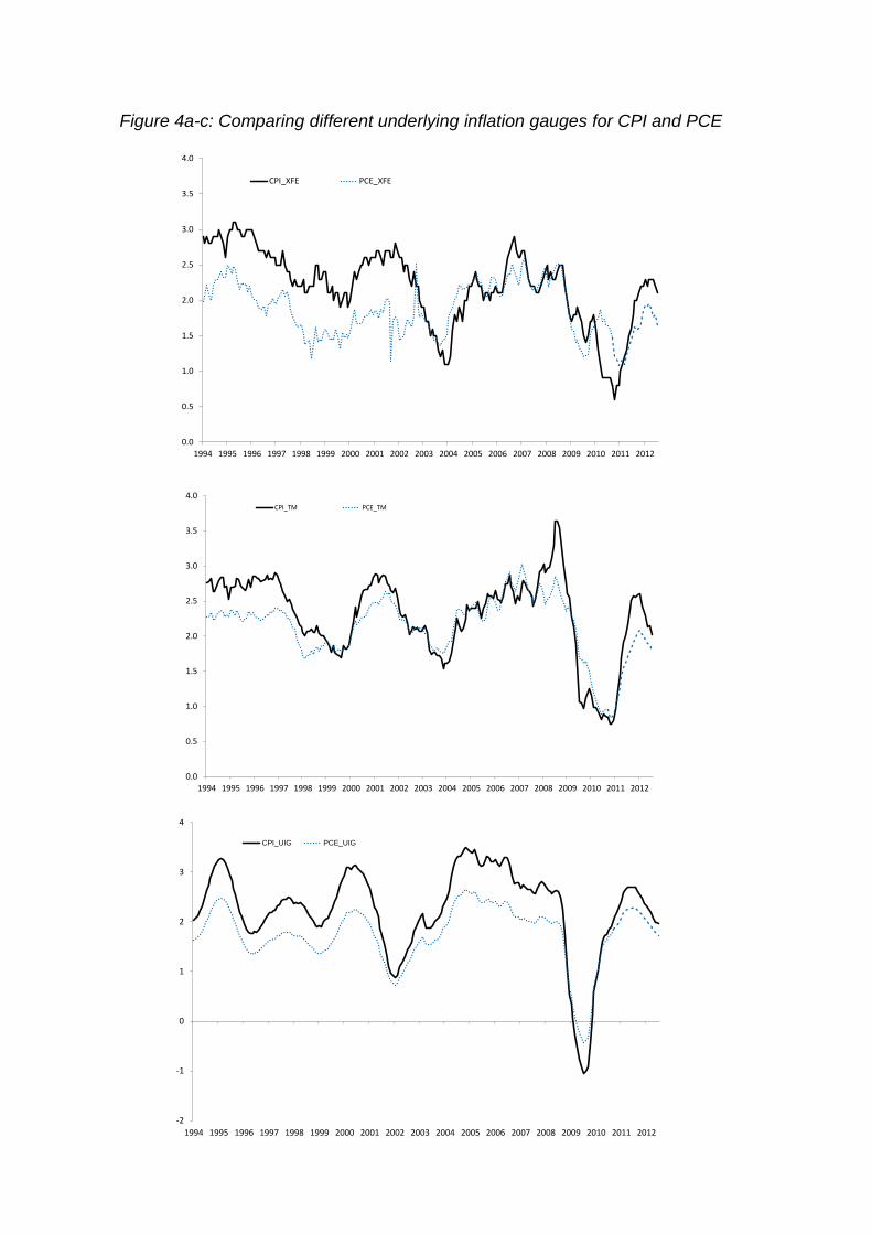
Figure 4a-c: Comparing different underlying inflation gauges for CPI and PCE

0.0

0.5

1.0

1.5

2.0

2.5

3.0

3.5

4.0

1994 1995 1996 1997 1998 1999 2000 2001 2002 2003 2004 2005 2006 2007 2008 2009 2010 2011 2012

CPI_XFE PCE_XFE

0.0

0.5

1.0

1.5

2.0

2.5

3.0

3.5

4.0

1994 1995 1996 1997 1998 1999 2000 2001 2002 2003 2004 2005 2006 2007 2008 2009 2010 2011 2012

CPI_TM PCE_TM

-2

-1

0

1

2

3

4

1994 1995 1996 1997 1998 1999 2000 2001 2002 2003 2004 2005 2006 2007 2008 2009 2010 2011 2012

CPI_UIG PCE_UIG

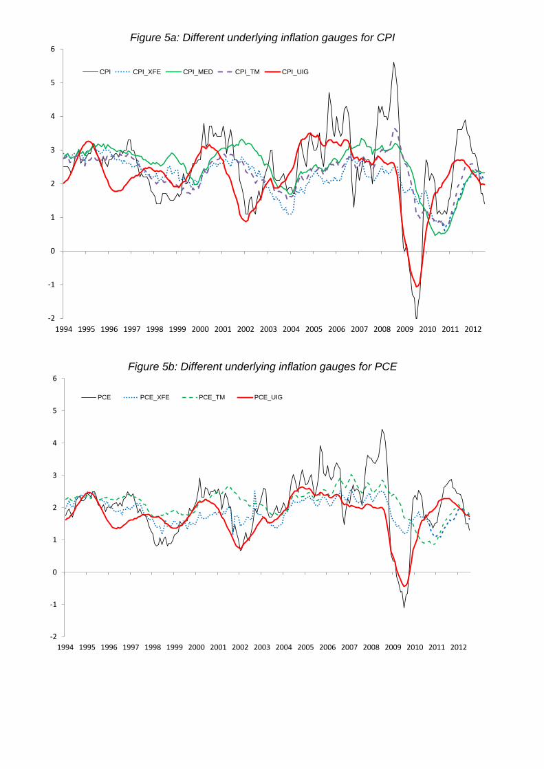
Figure 5a: Different underlying inflation gauges for CPI

-2

-1

0

1

2

3

4

5

6

1994 1995 1996 1997 1998 1999 2000 2001 2002 2003 2004 2005 2006 2007 2008 2009 2010 2011 2012

CPI CPI_XFE CPI_MED CPI_TM CPI_UIG

Figure 5b: Different underlying inflation gauges for PCE

-2

-1

0

1

2

3

4

5

6

1994 1995 1996 1997 1998 1999 2000 2001 2002 2003 2004 2005 2006 2007 2008 2009 2010 2011 2012

PCE PCE_XFE PCE_TM PCE_UIG

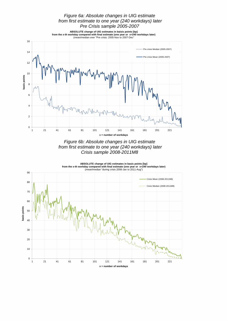
Figure 6a: Absolute changes in UIG estimate from first estimate to one year (240 workdays) later

Pre Crisis sample 2005-2007

0

2

4

6

8

10

12

14

16

1 21 41 61 81 101 121 141 161 181 201 221

basi

s po

ints

x = number of workdays

ABSOLUTE change of UIG estimates in baisis points [bp]from the x-th workday compared with final estimate (one year or x=240 workdays later)

(mean/median over "Pre crisis: 2005-Nov to 2007-Dec"

Pre crisis Median (2005-2007)

Pre crisis Mean (2005-2007)

Figure 6b: Absolute changes in UIG estimate

from first estimate to one year (240 workdays) later Crisis sample 2008-2011M8

0

10

20

30

40

50

60

70

80

90

1 21 41 61 81 101 121 141 161 181 201 221

basi

s po

ints

x = number of workdays

ABSOLUTE change of UIG estimates in basis points [bp]from the x-th workday compared with final estimate (one year or x=240 workdays later)

(mean/median "during crisis 2008-Jan to 2011-Aug")

Crisis Mean (2008-2011M8)

Crisis Median (2008-2011M8)

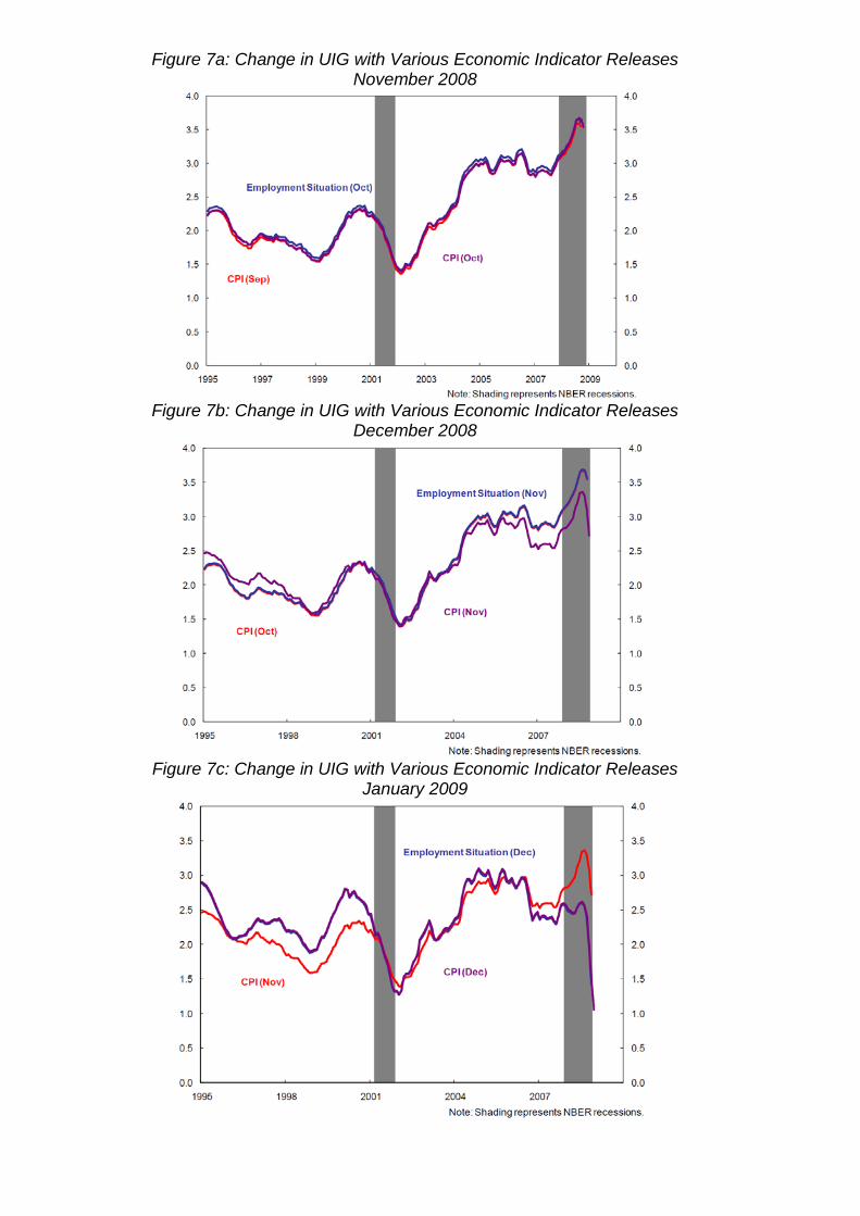
Figure 7a: Change in UIG with Various Economic Indicator Releases November 2008

Figure 7b: Change in UIG with Various Economic Indicator Releases

December 2008

Figure 7c: Change in UIG with Various Economic Indicator Releases

January 2009

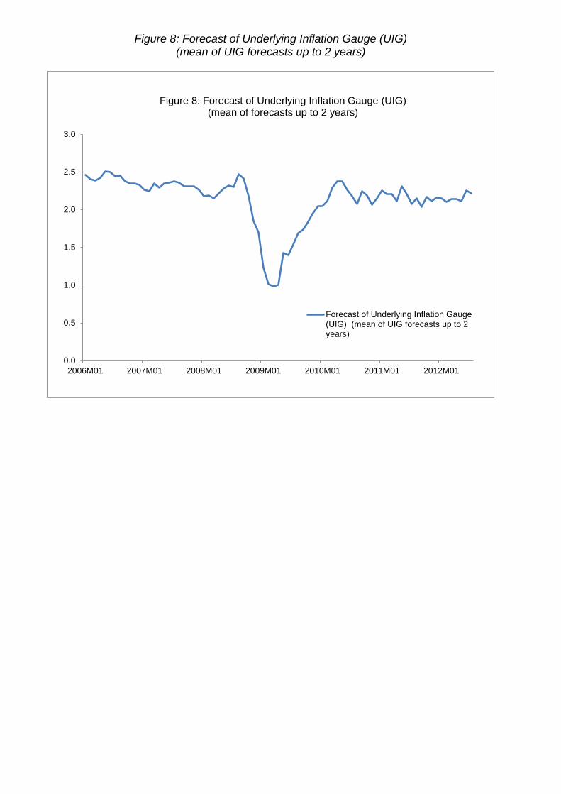
Figure 8: Forecast of Underlying Inflation Gauge (UIG) (mean of UIG forecasts up to 2 years)

0.0

0.5

1.0

1.5

2.0

2.5

3.0

2006M01 2007M01 2008M01 2009M01 2010M01 2011M01 2012M01

Figure 8: Forecast of Underlying Inflation Gauge (UIG) (mean of forecasts up to 2 years)

Forecast of Underlying Inflation Gauge(UIG) (mean of UIG forecasts up to 2years)

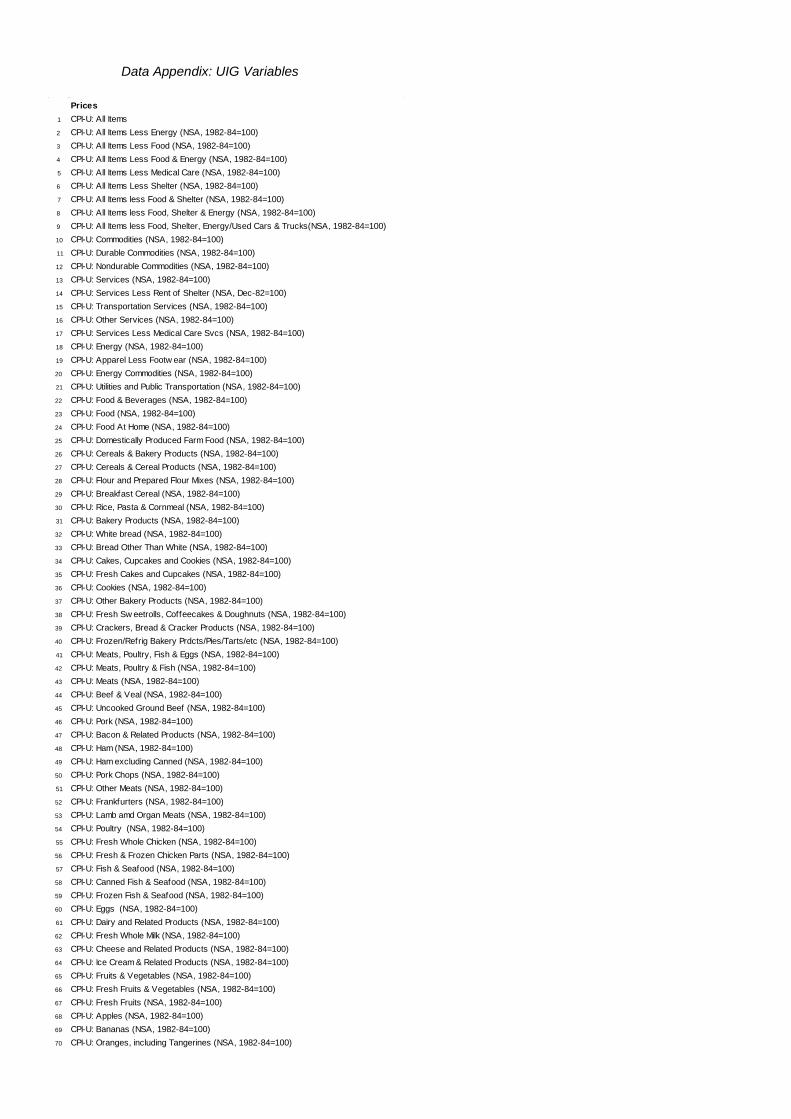
Data Appendix: UIG Variables

Prices1 CPI-U: All Items2 CPI-U: All Items Less Energy (NSA, 1982-84=100) 3 CPI-U: All Items Less Food (NSA, 1982-84=100) 4 CPI-U: All Items Less Food & Energy (NSA, 1982-84=100) 5 CPI-U: All Items Less Medical Care (NSA, 1982-84=100) 6 CPI-U: All Items Less Shelter (NSA, 1982-84=100) 7 CPI-U: All Items less Food & Shelter (NSA, 1982-84=100) 8 CPI-U: All Items less Food, Shelter & Energy (NSA, 1982-84=100) 9 CPI-U: All Items less Food, Shelter, Energy/Used Cars & Trucks(NSA, 1982-84=100) 10 CPI-U: Commodities (NSA, 1982-84=100) 11 CPI-U: Durable Commodities (NSA, 1982-84=100) 12 CPI-U: Nondurable Commodities (NSA, 1982-84=100) 13 CPI-U: Services (NSA, 1982-84=100) 14 CPI-U: Services Less Rent of Shelter (NSA, Dec-82=100) 15 CPI-U: Transportation Services (NSA, 1982-84=100) 16 CPI-U: Other Services (NSA, 1982-84=100) 17 CPI-U: Services Less Medical Care Svcs (NSA, 1982-84=100) 18 CPI-U: Energy (NSA, 1982-84=100) 19 CPI-U: Apparel Less Footw ear (NSA, 1982-84=100) 20 CPI-U: Energy Commodities (NSA, 1982-84=100) 21 CPI-U: Utilities and Public Transportation (NSA, 1982-84=100) 22 CPI-U: Food & Beverages (NSA, 1982-84=100) 23 CPI-U: Food (NSA, 1982-84=100) 24 CPI-U: Food At Home (NSA, 1982-84=100) 25 CPI-U: Domestically Produced Farm Food (NSA, 1982-84=100) 26 CPI-U: Cereals & Bakery Products (NSA, 1982-84=100) 27 CPI-U: Cereals & Cereal Products (NSA, 1982-84=100) 28 CPI-U: Flour and Prepared Flour Mixes (NSA, 1982-84=100) 29 CPI-U: Breakfast Cereal (NSA, 1982-84=100) 30 CPI-U: Rice, Pasta & Cornmeal (NSA, 1982-84=100) 31 CPI-U: Bakery Products (NSA, 1982-84=100) 32 CPI-U: White bread (NSA, 1982-84=100) 33 CPI-U: Bread Other Than White (NSA, 1982-84=100) 34 CPI-U: Cakes, Cupcakes and Cookies (NSA, 1982-84=100) 35 CPI-U: Fresh Cakes and Cupcakes (NSA, 1982-84=100) 36 CPI-U: Cookies (NSA, 1982-84=100) 37 CPI-U: Other Bakery Products (NSA, 1982-84=100) 38 CPI-U: Fresh Sw eetrolls, Coffeecakes & Doughnuts (NSA, 1982-84=100) 39 CPI-U: Crackers, Bread & Cracker Products (NSA, 1982-84=100) 40 CPI-U: Frozen/Refrig Bakery Prdcts/Pies/Tarts/etc (NSA, 1982-84=100) 41 CPI-U: Meats, Poultry, Fish & Eggs (NSA, 1982-84=100) 42 CPI-U: Meats, Poultry & Fish (NSA, 1982-84=100) 43 CPI-U: Meats (NSA, 1982-84=100) 44 CPI-U: Beef & Veal (NSA, 1982-84=100) 45 CPI-U: Uncooked Ground Beef (NSA, 1982-84=100) 46 CPI-U: Pork (NSA, 1982-84=100) 47 CPI-U: Bacon & Related Products (NSA, 1982-84=100) 48 CPI-U: Ham (NSA, 1982-84=100) 49 CPI-U: Ham excluding Canned (NSA, 1982-84=100) 50 CPI-U: Pork Chops (NSA, 1982-84=100) 51 CPI-U: Other Meats (NSA, 1982-84=100) 52 CPI-U: Frankfurters (NSA, 1982-84=100) 53 CPI-U: Lamb amd Organ Meats (NSA, 1982-84=100) 54 CPI-U: Poultry (NSA, 1982-84=100) 55 CPI-U: Fresh Whole Chicken (NSA, 1982-84=100) 56 CPI-U: Fresh & Frozen Chicken Parts (NSA, 1982-84=100) 57 CPI-U: Fish & Seafood (NSA, 1982-84=100) 58 CPI-U: Canned Fish & Seafood (NSA, 1982-84=100) 59 CPI-U: Frozen Fish & Seafood (NSA, 1982-84=100) 60 CPI-U: Eggs (NSA, 1982-84=100) 61 CPI-U: Dairy and Related Products (NSA, 1982-84=100) 62 CPI-U: Fresh Whole Milk (NSA, 1982-84=100) 63 CPI-U: Cheese and Related Products (NSA, 1982-84=100) 64 CPI-U: Ice Cream & Related Products (NSA, 1982-84=100) 65 CPI-U: Fruits & Vegetables (NSA, 1982-84=100) 66 CPI-U: Fresh Fruits & Vegetables (NSA, 1982-84=100) 67 CPI-U: Fresh Fruits (NSA, 1982-84=100) 68 CPI-U: Apples (NSA, 1982-84=100) 69 CPI-U: Bananas (NSA, 1982-84=100) 70 CPI-U: Oranges, including Tangerines (NSA, 1982-84=100)

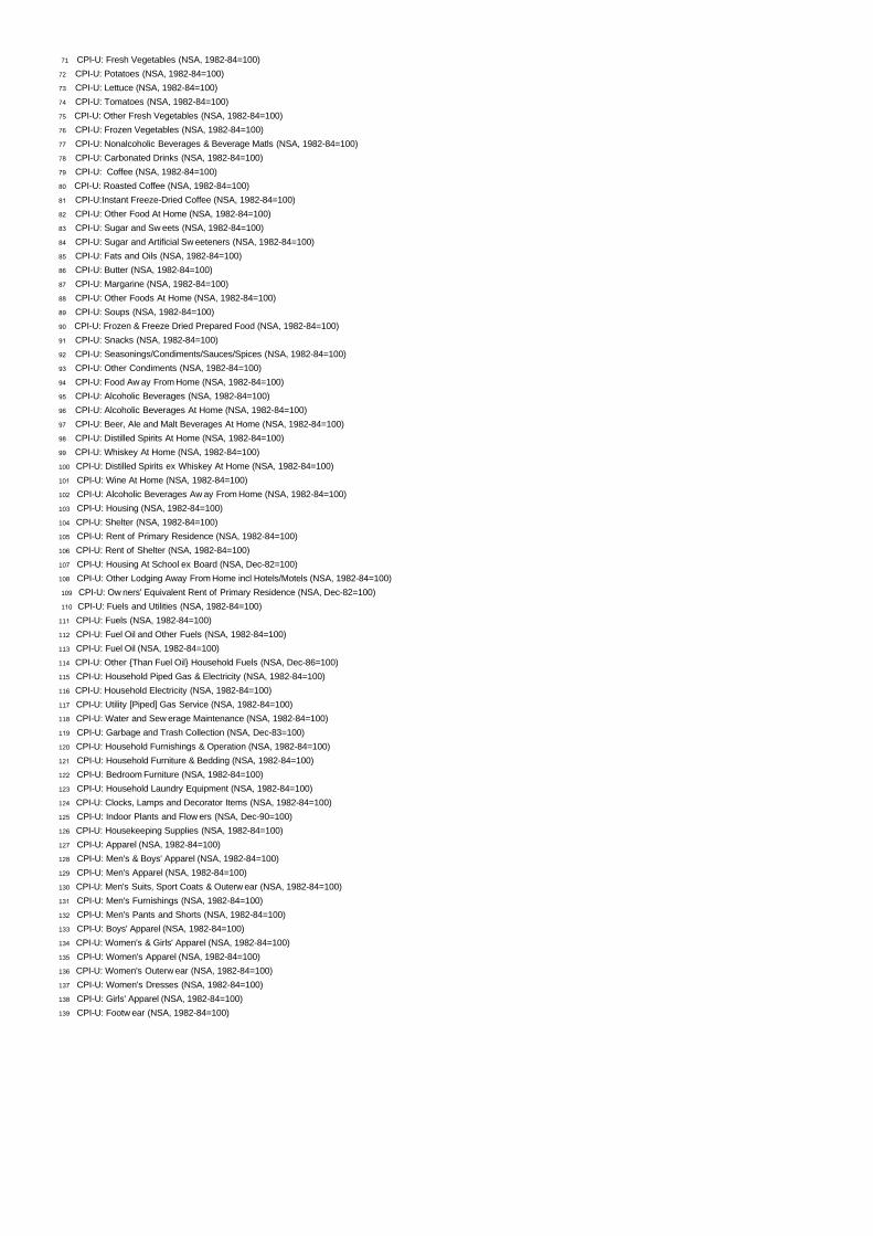
71 CPI-U: Fresh Vegetables (NSA, 1982-84=100) 72 CPI-U: Potatoes (NSA, 1982-84=100) 73 CPI-U: Lettuce (NSA, 1982-84=100) 74 CPI-U: Tomatoes (NSA, 1982-84=100) 75 CPI-U: Other Fresh Vegetables (NSA, 1982-84=100) 76 CPI-U: Frozen Vegetables (NSA, 1982-84=100) 77 CPI-U: Nonalcoholic Beverages & Beverage Matls (NSA, 1982-84=100) 78 CPI-U: Carbonated Drinks (NSA, 1982-84=100) 79 CPI-U: Coffee (NSA, 1982-84=100) 80 CPI-U: Roasted Coffee (NSA, 1982-84=100) 81 CPI-U:Instant Freeze-Dried Coffee (NSA, 1982-84=100) 82 CPI-U: Other Food At Home (NSA, 1982-84=100) 83 CPI-U: Sugar and Sw eets (NSA, 1982-84=100) 84 CPI-U: Sugar and Artificial Sw eeteners (NSA, 1982-84=100) 85 CPI-U: Fats and Oils (NSA, 1982-84=100) 86 CPI-U: Butter (NSA, 1982-84=100) 87 CPI-U: Margarine (NSA, 1982-84=100) 88 CPI-U: Other Foods At Home (NSA, 1982-84=100) 89 CPI-U: Soups (NSA, 1982-84=100) 90 CPI-U: Frozen & Freeze Dried Prepared Food (NSA, 1982-84=100) 91 CPI-U: Snacks (NSA, 1982-84=100) 92 CPI-U: Seasonings/Condiments/Sauces/Spices (NSA, 1982-84=100) 93 CPI-U: Other Condiments (NSA, 1982-84=100) 94 CPI-U: Food Aw ay From Home (NSA, 1982-84=100) 95 CPI-U: Alcoholic Beverages (NSA, 1982-84=100) 96 CPI-U: Alcoholic Beverages At Home (NSA, 1982-84=100) 97 CPI-U: Beer, Ale and Malt Beverages At Home (NSA, 1982-84=100) 98 CPI-U: Distilled Spirits At Home (NSA, 1982-84=100) 99 CPI-U: Whiskey At Home (NSA, 1982-84=100) 100 CPI-U: Distilled Spirits ex Whiskey At Home (NSA, 1982-84=100) 101 CPI-U: Wine At Home (NSA, 1982-84=100) 102 CPI-U: Alcoholic Beverages Aw ay From Home (NSA, 1982-84=100) 103 CPI-U: Housing (NSA, 1982-84=100) 104 CPI-U: Shelter (NSA, 1982-84=100) 105 CPI-U: Rent of Primary Residence (NSA, 1982-84=100) 106 CPI-U: Rent of Shelter (NSA, 1982-84=100) 107 CPI-U: Housing At School ex Board (NSA, Dec-82=100) 108 CPI-U: Other Lodging Away From Home incl Hotels/Motels (NSA, 1982-84=100) 109 CPI-U: Ow ners' Equivalent Rent of Primary Residence (NSA, Dec-82=100)110 CPI-U: Fuels and Utilities (NSA, 1982-84=100)

111 CPI-U: Fuels (NSA, 1982-84=100) 112 CPI-U: Fuel Oil and Other Fuels (NSA, 1982-84=100) 113 CPI-U: Fuel Oil (NSA, 1982-84=100) 114 CPI-U: Other {Than Fuel Oil} Household Fuels (NSA, Dec-86=100) 115 CPI-U: Household Piped Gas & Electricity (NSA, 1982-84=100) 116 CPI-U: Household Electricity (NSA, 1982-84=100) 117 CPI-U: Utility [Piped] Gas Service (NSA, 1982-84=100) 118 CPI-U: Water and Sew erage Maintenance (NSA, 1982-84=100) 119 CPI-U: Garbage and Trash Collection (NSA, Dec-83=100) 120 CPI-U: Household Furnishings & Operation (NSA, 1982-84=100) 121 CPI-U: Household Furniture & Bedding (NSA, 1982-84=100) 122 CPI-U: Bedroom Furniture (NSA, 1982-84=100) 123 CPI-U: Household Laundry Equipment (NSA, 1982-84=100) 124 CPI-U: Clocks, Lamps and Decorator Items (NSA, 1982-84=100) 125 CPI-U: Indoor Plants and Flow ers (NSA, Dec-90=100) 126 CPI-U: Housekeeping Supplies (NSA, 1982-84=100) 127 CPI-U: Apparel (NSA, 1982-84=100) 128 CPI-U: Men's & Boys' Apparel (NSA, 1982-84=100) 129 CPI-U: Men's Apparel (NSA, 1982-84=100) 130 CPI-U: Men's Suits, Sport Coats & Outerw ear (NSA, 1982-84=100) 131 CPI-U: Men's Furnishings (NSA, 1982-84=100) 132 CPI-U: Men's Pants and Shorts (NSA, 1982-84=100) 133 CPI-U: Boys' Apparel (NSA, 1982-84=100) 134 CPI-U: Women's & Girls' Apparel (NSA, 1982-84=100) 135 CPI-U: Women's Apparel (NSA, 1982-84=100) 136 CPI-U: Women's Outerw ear (NSA, 1982-84=100) 137 CPI-U: Women's Dresses (NSA, 1982-84=100) 138 CPI-U: Girls' Apparel (NSA, 1982-84=100) 139 CPI-U: Footw ear (NSA, 1982-84=100)

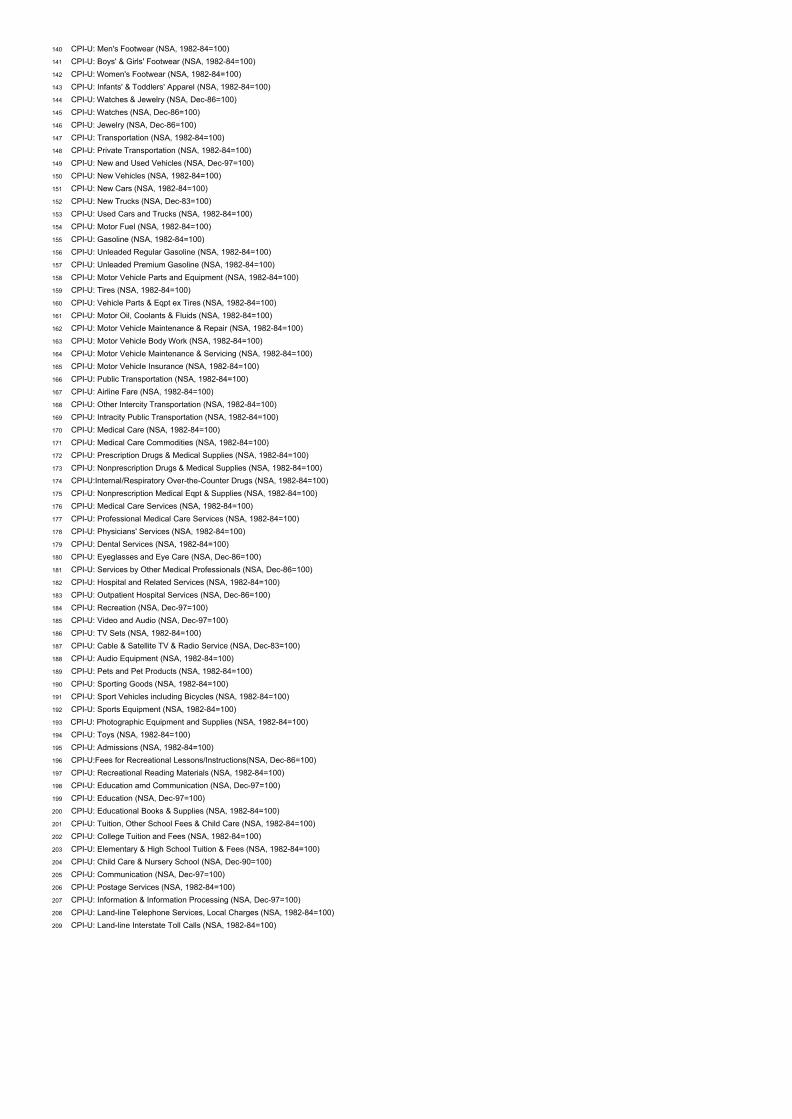
140 CPI-U: Men's Footwear (NSA, 1982-84=100)

141 CPI-U: Boys' & Girls' Footwear (NSA, 1982-84=100)

142 CPI-U: Women's Footwear (NSA, 1982-84=100)

143 CPI-U: Infants' & Toddlers' Apparel (NSA, 1982-84=100)

144 CPI-U: Watches & Jewelry (NSA, Dec-86=100)

145 CPI-U: Watches (NSA, Dec-86=100)

146 CPI-U: Jewelry (NSA, Dec-86=100)

147 CPI-U: Transportation (NSA, 1982-84=100)

148 CPI-U: Private Transportation (NSA, 1982-84=100)

149 CPI-U: New and Used Vehicles (NSA, Dec-97=100)

150 CPI-U: New Vehicles (NSA, 1982-84=100)

151 CPI-U: New Cars (NSA, 1982-84=100)

152 CPI-U: New Trucks (NSA, Dec-83=100)

153 CPI-U: Used Cars and Trucks (NSA, 1982-84=100)

154 CPI-U: Motor Fuel (NSA, 1982-84=100)

155 CPI-U: Gasoline (NSA, 1982-84=100)

156 CPI-U: Unleaded Regular Gasoline (NSA, 1982-84=100)

157 CPI-U: Unleaded Premium Gasoline (NSA, 1982-84=100)

158 CPI-U: Motor Vehicle Parts and Equipment (NSA, 1982-84=100)

159 CPI-U: Tires (NSA, 1982-84=100)

160 CPI-U: Vehicle Parts & Eqpt ex Tires (NSA, 1982-84=100)

161 CPI-U: Motor Oil, Coolants & Fluids (NSA, 1982-84=100)

162 CPI-U: Motor Vehicle Maintenance & Repair (NSA, 1982-84=100)

163 CPI-U: Motor Vehicle Body Work (NSA, 1982-84=100)

164 CPI-U: Motor Vehicle Maintenance & Servicing (NSA, 1982-84=100)

165 CPI-U: Motor Vehicle Insurance (NSA, 1982-84=100)

166 CPI-U: Public Transportation (NSA, 1982-84=100)

167 CPI-U: Airline Fare (NSA, 1982-84=100)

168 CPI-U: Other Intercity Transportation (NSA, 1982-84=100)

169 CPI-U: Intracity Public Transportation (NSA, 1982-84=100)

170 CPI-U: Medical Care (NSA, 1982-84=100)

171 CPI-U: Medical Care Commodities (NSA, 1982-84=100)

172 CPI-U: Prescription Drugs & Medical Supplies (NSA, 1982-84=100)

173 CPI-U: Nonprescription Drugs & Medical Supplies (NSA, 1982-84=100)

174 CPI-U:Internal/Respiratory Over-the-Counter Drugs (NSA, 1982-84=100)

175 CPI-U: Nonprescription Medical Eqpt & Supplies (NSA, 1982-84=100)

176 CPI-U: Medical Care Services (NSA, 1982-84=100)

177 CPI-U: Professional Medical Care Services (NSA, 1982-84=100)

178 CPI-U: Physicians' Services (NSA, 1982-84=100)

179 CPI-U: Dental Services (NSA, 1982-84=100)

180 CPI-U: Eyeglasses and Eye Care (NSA, Dec-86=100)

181 CPI-U: Services by Other Medical Professionals (NSA, Dec-86=100)

182 CPI-U: Hospital and Related Services (NSA, 1982-84=100)

183 CPI-U: Outpatient Hospital Services (NSA, Dec-86=100)

184 CPI-U: Recreation (NSA, Dec-97=100)

185 CPI-U: Video and Audio (NSA, Dec-97=100)

186 CPI-U: TV Sets (NSA, 1982-84=100)

187 CPI-U: Cable & Satellite TV & Radio Service (NSA, Dec-83=100)

188 CPI-U: Audio Equipment (NSA, 1982-84=100)

189 CPI-U: Pets and Pet Products (NSA, 1982-84=100)

190 CPI-U: Sporting Goods (NSA, 1982-84=100)

191 CPI-U: Sport Vehicles including Bicycles (NSA, 1982-84=100)

192 CPI-U: Sports Equipment (NSA, 1982-84=100)

193 CPI-U: Photographic Equipment and Supplies (NSA, 1982-84=100)

194 CPI-U: Toys (NSA, 1982-84=100)

195 CPI-U: Admissions (NSA, 1982-84=100)

196 CPI-U:Fees for Recreational Lessons/Instructions(NSA, Dec-86=100)

197 CPI-U: Recreational Reading Materials (NSA, 1982-84=100)

198 CPI-U: Education amd Communication (NSA, Dec-97=100)

199 CPI-U: Education (NSA, Dec-97=100)

200 CPI-U: Educational Books & Supplies (NSA, 1982-84=100)

201 CPI-U: Tuition, Other School Fees & Child Care (NSA, 1982-84=100)

202 CPI-U: College Tuition and Fees (NSA, 1982-84=100)

203 CPI-U: Elementary & High School Tuition & Fees (NSA, 1982-84=100)

204 CPI-U: Child Care & Nursery School (NSA, Dec-90=100)

205 CPI-U: Communication (NSA, Dec-97=100)

206 CPI-U: Postage Services (NSA, 1982-84=100)

207 CPI-U: Information & Information Processing (NSA, Dec-97=100)

208 CPI-U: Land-line Telephone Services, Local Charges (NSA, 1982-84=100)

209 CPI-U: Land-line Interstate Toll Calls (NSA, 1982-84=100)

210 CPI-U: Land-line Intrastate Toll Calls (NSA, 1982-84=100) 211 CPI-U: Information Technology, Hardw are, & Services (NSA, Dec 1988=100) 212 CPI-U: Other Goods & Services (NSA, 1982-84=100) 213 CPI-U: Tobacco & Smoking Products (NSA, 1982-84=100) 214 CPI-U: Personal Care (NSA, 1982-84=100) 215 CPI-U: Personal Care Products (NSA, 1982-84=100) 216 CPI-U: Cosmetics/Perfumes/Bath/Nail Preps & Impls(NSA, 1982-84=100) 217 CPI-U: Personal Care Services (NSA, 1982-84=100) 218 CPI-U: Miscellaneous Personal Services (NSA, 1982-84=100) 219 CPI-U: Legal Services (NSA, Dec-86=100) 220 CPI-U: Funeral Expenses (NSA, Dec-86=100) 221 CPI-U: Financial Services (NSA, Dec-86=100) 222 CPI-U: Stationery/Stationery Supplies/Gift Wrap (NSA, 1982-84=100) 223 PPI: Finished Consumer Goods (NSA, 1982=100)224 PPI: Finished Consumer Foods (NSA, 1982=100)225 PPI: Finished Consumer Foods: Unprocessed (NSA, 1982=100)226 PPI: Finished Consumer Foods; Processed (NSA, 1982=100)227 PPI: Finished Consumer Goods excluding Foods (NSA, 1982=100)228 PPI: Consumer Nondurable Goods Less Food (NSA,1982=100)229 PPI: Consumer Durable Goods (NSA, 1982=100)230 PPI: Finished Capital Equipment (NSA, 1982=100)231 PPI: Capital Equipment: Manufacturing Industries (NSA, 1982=100)232 PPI: Capital Equipment: Nonmanufacturing Industries (NSA, 1982=100) 233 PPI: Finished Goods [Including Foods & Fuel] (NSA, 1982=100)234 PPI: Intermediate Materials, Supplies & Components (NSA, 1982=100) 235 PPI: Crude Materials For Further Processing (NSA, 1982=100)236 PPI: Finished Goods excluding Foods (NSA, 1982=100)237 PPI: Offices of Physicians (Dec-96=100)238 PPI: Home Health Care Services (Dec-96=100)239 PPI: Commercial Natural Gas (NSA, Dec-90=100)240 Import Price Index: All Imports (NSA, 2000=100)241 Export Price Index: All Exports (NSA, 2000=100)242 FRB Dallas Trimmed-Mean 12-month PCE Inflation Rate (%)

Real Variables1 ISM: Mfg: New Orders Index (NSA, 50+ = Econ Expand)2 ISM: Mfg: Production Index (NSA, 50+ = Econ Expand)3 ISM: Mfg: Employment Index (NSA, 50+ = Econ Expand)4 ISM: Mfg: Vendor Deliveries Index (NSA, 50+ = Econ Expand)5 ISM: Mfg: Inventories Index (NSA, 50+ = Econ Expand)6 ISM: Mfg: Prices Index (NSA, 50+ = Econ Expand)7 ISM: Mfg: Backlog of Orders Index (NSA, 50+=Econ Expand)8 ISM: Mfg: New Export Orders Index(NSA, 50+ = Econ Expand)9 ISM: Mfg: Imports Index (NSA, 50+ = Econ Expand)10 ISM: Nonmfg: New Orders Index (NSA, 50+ = Econ Expand)11 ISM: Nonmfg: Business Activity Index (NSA, 50+ = Econ Expand)12 ISM: Nonmfg: Employment Index (NSA, 50+ = Econ Expand)13 ISM: Nonmfg: Supplier Deliveries Index (NSA, 50+ = Econ Expand)14 ISM: Nonmfg: Inventory Change Index (NSA, 50+ =Econ Expand)15 ISM: Nonmfg: Prices Index (NSA, 50+ = Econ Expand)16 ISM: Nonmfg: Orders Backlog Index (NSA, 50+ = Econ Expand)17 ISM: Nonmfg: New Export Orders Index (NSA, 50+=Econ Expand)18 ISM: Nonmfg: Imports Index (NSA, 50+ = Econ Expand)

Labor1 Unemployment Rate: 16-24 Yrs (NSA, %)2 Unemployment Rate: 25-34 Yrs (NSA, %)3 Unemployment Rate: 35-44 Yrs (NSA, %)4 Unemployment Rate: 45-54 Yrs (NSA, %)5 Unemployment Rate: 55 Yrs & Over (NSA, %)6 Civilian Employment-Population Ratio: 16-24 Yrs (NSA, Ratio)7 Civilian Employment-Population Ratio: 25 to 34 Yrs (NSA, Ratio)8 Civilian Employment-Population Ratio: 35 to 44 Yrs (NSA, Ratio)9 Civilian Employment-Population Ratio: 45 to 54 Yrs (NSA, Ratio)10 Civilian Employment-Population Ratio: 55 Yrs & Over (NSA, Ratio)11 Average Weeks Unemployed: 16-19 yrs (NSA)12 Average Weeks Unemployed: 20-24 yrs (NSA)13 Average Weeks Unemployed: 25-34 yrs (NSA)14 Average Weeks Unemployed: 35-44 yrs (NSA)15 Average Weeks Unemployed: 45-54 yrs (NSA)16 Average Weeks Unemployed: 55-64 yrs (NSA)17 Average Weeks Unemployed: 65 yrs & over (NSA)18 Unemployment (NSA, Thous)19 Number Unemployed for less than 5 Weeks (NSA, Thous)20 Number Unemployed for 5-14 Weeks (NSA, Thous)21 Number Unemployed for 15-26 Weeks (NSA, Thous)22 Number Unemployed for 15 Weeks & Over (NSA, Thous)23 Unemployment Insurance: Initial Claims (#, NSA)

Money1 Money Stock: M1 (NSA, Bil.$)2 Money Stock: M2 (NSA, Bil.$)3 Adjusted Monetary Base (NSA, Mil.$)4 Adjusted Reserves of Depository Institutions (NSA, Mil.$)5 Adjusted Nonborrow ed Reserves of Depository Institutions (NSA, Mil.$)

Financials1 Cash Price: Gold Bullion, London Commodity Price, PM Fix (US$/troy Oz)2 Gold: London PM Fix (US$/Troy Oz)3 Gold Spot ($/oz) NSA4 Spot commodity price - West Texas Intermediate crude oil, Cushing OK5 Federal funds effective rate6 3-month Treasury bill rate coupon equivalent7 6-month Treasury bill rate coupon equivalent8 1-Year Treasury Bill Yield at Constant Maturity (% p.a.)9 5-Year Treasury Note Yield at Constant Maturity (% p.a.)10 7-Year Treasury Note Yield at Constant Maturity (% p.a.)11 10-Year Treasury Note Yield at Constant Maturity (% p.a.)12 LIBOR Eurodollar 11 A.M. Fixing 1 Month13 LIBOR Eurodollar 11 A.M. Fixing 3 Month14 LIBOR Eurodollar 11 A.M. Fixing 6 Month15 LIBOR Eurodollar 11 A.M. Fixing 9 Month16 LIBOR Eurodollar 11 A.M. Fixing 1 Year17 Spot Price (Eur/$) (Revised Backw ards)18 Spot Price (GBP/$)19 Spot Price (Yen/$)20 Spot Price (Sw iss Franc/$)21 Board Narrow Nominal Effective Exchange Rate Index: U.S. (2000=100)22 Board Broad Nominal Effective Exchange Rate: United States (2000=100)23 Bank Credit: All Commercial Banks (NSA, Bil.$)24 Total Revolving U.S. Consumer Credit Outstanding25 Total Non-Revolving U.S. Consumer Credit Outstanding26 Securities in Bank Credit: All Commercial Banks (NSA, Bil.$)27 US Government Securities in Bank Credit:All Commercial Banks (NSA,Bil$)28 Real Estate Loans in Bank Credit: All Commercial Banks (NSA, Bil.$)29 C & I Loans in Bank Credit: All Commercial Banks (NSA, Bil.$)30 Consumer Loans in Bank Credit: All Commercial Banks (NSA, Bil.$)31 Moody's Seasoned Aaa Corporate Bond Yield (% p.a.)32 Moody's Seasoned Baa Corporate Bond Yield (% p.a.)33 Merrill Lynch High Yield Master II yield 34 New York Stock Exchange Composite Index35 New York Stock Exchange Total Volume36 Standard and Poor's 500 Price Earnings Ratio Index37 Dow Jones Industrial Average38 Dow Jones Wilshire 5000 Composite Index Full Cap39 Light Sw eet Crude Oil Futures Price: 1st Exp Contract Nearby Sttlmnt (EOP,$/bbl)40 Light Sw eet Crude Oil Futures Price: 3 Month Contract Settlement (EOP, $/bbl)41 Light Sw eet Crude Oil Futures Price: 6 Month Contract Settlement (EOP, $/bbl)42 No 2 Heating Oil Futures Price: 1st Exp Contract Nearby Settlement (EOP, $/gal)43 No 2 Heating Oil Futures Price: 3 Month Contract Settlement (EOP, $/gal)44 No 2 Heating Oil Futures Price: 6 Month Contract Settlement (EOP, $/gal)45 Unleaded Gasoline Futures Price: 1st Exp Contract Nearby Settlement (EOP, $/gal)46 Unleaded Gasoline Futures Price: 3 Month Contract Settlement (EOP, $/gal)47 New York Harbor Conventional Gasoline Regular Spot Price FOB (EOP Cents/Gallon) 48 Gas Oil Futures Price: 1st Exp Contract Nearby Settlement ($/metric tEOP, on)49 Unleaded Premium Gasoline Price, NY gal (EOP, $/gal)50 Unleaded Gas, Regular, Non-Oxygenated: NY (EOP, $/gal)51 Natural Gas Price, Henry Hub, LA ($/mmbtu)52 Dow Jones AIG Futures Price Index (Jan-2-91=100)53 Dow Jones AIG Spot Price Index (Jan-7-91=100)54 FIBER Industrial Materials Index: All Items (1990=100)55 Goldman Sachs Commodity Nearby Index (EOP, Dec-31-69=100)56 S&P 500 Futures Price: 1st Exp Contract Nearby Settlement (EOP, Index)57 S&P 400 Midcap Futures Price: 1st Exp Contract Nearby Settlement (EOP, Index)

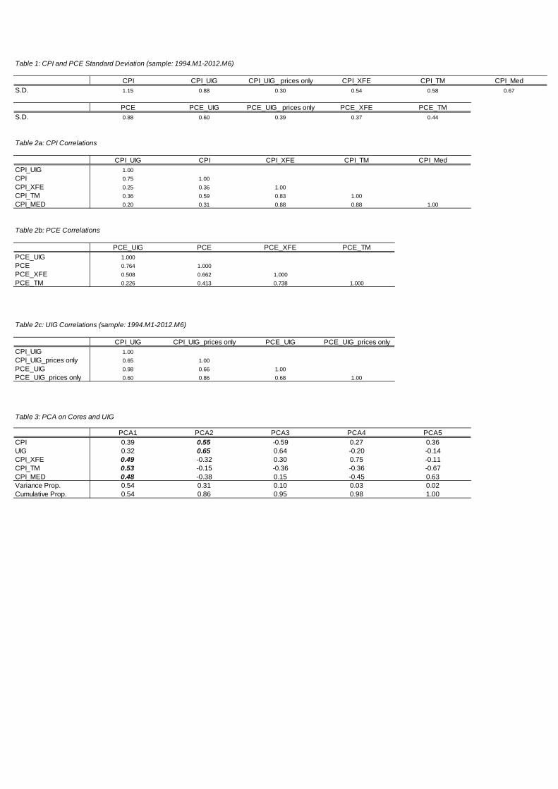
Table 1: CPI and PCE Standard Deviation (sample: 1994.M1-2012.M6)

CPI CPI_UIG CPI_UIG_ prices only CPI_XFE CPI_TM CPI_MedS.D. 1.15 0.88 0.30 0.54 0.58 0.67

PCE PCE_UIG PCE_UIG_ prices only PCE_XFE PCE_TMS.D. 0.88 0.60 0.39 0.37 0.44

Table 2a: CPI Correlations

CPI_UIG CPI CPI_XFE CPI_TM CPI_MedCPI_UIG 1.00CPI 0.75 1.00CPI_XFE 0.25 0.36 1.00CPI_TM 0.36 0.59 0.83 1.00CPI_MED 0.20 0.31 0.88 0.88 1.00

Table 2b: PCE Correlations

PCE_UIG PCE PCE_XFE PCE_TMPCE_UIG 1.000PCE 0.764 1.000PCE_XFE 0.508 0.662 1.000PCE_TM 0.226 0.413 0.738 1.000

Table 2c: UIG Correlations (sample: 1994.M1-2012.M6)

CPI_UIG CPI_UIG_prices only PCE_UIG PCE_UIG_prices onlyCPI_UIG 1.00CPI_UIG_prices only 0.65 1.00PCE_UIG 0.98 0.66 1.00PCE_UIG_prices only 0.60 0.86 0.68 1.00

Table 3: PCA on Cores and UIG

PCA1 PCA2 PCA3 PCA4 PCA5CPI 0.39 0.55 -0.59 0.27 0.36UIG 0.32 0.65 0.64 -0.20 -0.14CPI_XFE 0.49 -0.32 0.30 0.75 -0.11CPI_TM 0.53 -0.15 -0.36 -0.36 -0.67CPI_MED 0.48 -0.38 0.15 -0.45 0.63Variance Prop. 0.54 0.31 0.10 0.03 0.02Cumulative Prop. 0.54 0.86 0.95 0.98 1.00

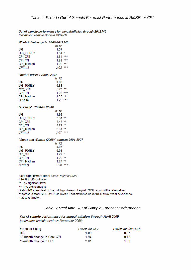
Table 4: Pseudo Out-of-Sample Forecast Performance in RMSE for CPI

Table 5: Real-time Out-of-Sample Forecast Performance