The fragile capital structure of hedge funds and the limits to

arbitrage�

Xuewen Liuy Antonio S. Mello

HKUST Wisconsin School of Business

Forthcoming in Journal of Financial Economics

Abstract

During a �nancial crisis, when investors are most in need of liquidity and accurate prices,

hedge funds cut their arbitrage positions and hoard cash. The paper explains this phenomenon.

We argue that the fragile nature of the capital structure of hedge funds, combined with low

market liquidity, creates a risk of coordination in redemptions among hedge fund investors that

severely limits hedge funds�arbitrage capabilities. We present a model of hedge funds�optimal

asset allocation in the presence of coordination risk among investors. We show that hedge

fund managers behave conservatively and even abstain from participating in the market once

coordination risk is factored into their investment decisions. The model suggests a new source

of limits to arbitrage

JEL classi�cation: G14; G24; D82

Keywords: Limits to arbitrage; Coordination risk; Fragile capital structure; Market liquidity

�We thank Sudipto Bhattacharya, Enrico Bi¢ s, Robert Kosowski, Tianxi Wang, seminar participants at the 2009

Imperial College hedge fund conference, and, in particular, Amil Dasgupa (the discussant) for helpful comments. We

are very grateful to the referee for detailed comments and suggestions that signi�cantly improved the paper.yCorresponding author. E-mail address: Xuewenliu@ust.hk (X. Liu).

1

�One fund-of-funds manager says he rushes to be the �rst out if he suspects that others may

desert a hedge fund. ... If managers [of hedge funds] worry that clients will bail out, they may try

to raise cash in anticipation.�

Economist, October 25, 2008, pp. 87�88.

1 Introduction

In the �nancial crisis of 2007�2009, hedge funds reduced their exposures to risky investments and

increased their cash holdings very quickly. The Economist estimates that between July and August

2008 alone, the industry�s cash holdings rose from $156 billion to a record $184 billion, equivalent

to 11% of assets under management.1 The reallocation toward cash seemed to be in anticipation of

unprecedented pressure for redemptions from investors. In fact, the hedge fund industry experienced

record levels of redemptions during the third and fourth quarters of 2008. In the �rst half of 2009,

investors continued to pull money out of hedge funds. Ironically, redemptions appear to have been

self-reinforcing. A report titled Hedge Funds 2009 by the International Financial Services London

Research (IFSL) says:

Hedge funds faced unprecedented pressure for redemptions in the latter part of 2008, with

investors withdrawing funds due to dissatisfaction with the performance or to cover for even greater

losses or cash calls elsewhere. This in turn led to forced selling and closures of positions by

hedge funds causing a cycle of further losses and redemptions. Some funds were not able to meet

withdrawal requests so were forced to suspend redemptions, as selling illiquid assets would have

damaged the investors that remained.

In this paper we ask why hedge funds, with a reputation for being aggressive investors seeking

high returns, hold signi�cant amounts of cash in their balance sheets. And, why do they quickly

increase their cash holdings (hoard liquidity) when a crisis strikes? One would think that it is

precisely during times of high uncertainty and high volatility that arbitrage opportunities are

greater.2 Why then do hedge funds become much less aggressive in exploiting price distortions and1�Hedge funds in trouble: the incredible shrinking funds,�Economist, October 25, 2008, pp. 87�88.2Mitchell and Pulvino (2011) and Krishnamurthy (2010) provide convincing evidence that, during the recent

liquidity crisis, arbitrage opportunities were pronounced in debt markets.

2

pass up pro�t opportunities?

In their quest for arbitrage gains, hedge funds also perform the important social role of enforcing

market e¢ ciency. From a social welfare point of view, it is not optimal that hedge funds allocate

large fractions of their portfolios to riskless securities, instead of pursuing arbitrage opportunities

in risky assets. Holding cash is synonymous with imposing limits on arbitrage. With insu¢ cient

arbitrage trading, �nancial markets can wander o¤ erratically and risk falling into a vicious cycle

that goes from lower price informativeness to less liquidity and back, a process of continued deteri-

oration that can prolong a �nancial crisis. Thus, to analyze a modern �nancial crisis it is necessary

to understand the reasons that hedge funds limit their arbitrage activities.

So far the �nance literature has associated the limits to arbitrage with investor uncertainty

about the fundamental value of the assets held by arbitrageurs. According to Shleifer and Vishny

(1997), when investors do not understand or observe perfectly arbitrageurs�trading positions, they

can react with their feet after observing poor performance. Understanding that poor performance

can cause redemptions, hedge fund managers refrain from making investments that might lose

money in the short term, even if a pro�t could be realized in the long run.3

In this paper, we o¤er an alternative explanation for the limits of arbitrage. We highlight

investors�concerns about coordination risk (i.e., the uncertainty about what other investors might

decide to do), instead of about fundamental risk. One key feature of the capital structure of hedge

funds is the fragile nature of their equity. Equity capital in hedge funds can be redeemed at investors�

discretion, a feature somewhat similar to demand deposit-debt in banks.4 The fragile equity capital

in hedge funds introduces the risk of coordination among hedge fund investors. The coordination

risk arises because investors suspect that other investors might redeem, and to meet redemptions

the hedge fund may be forced to liquidate positions at a loss. If investors suspect that, after

3Gromb and Vayanos (2002) build on the intuition of Shleifer and Vishny (1997) and show that margin constraints

have a similar e¤ect in limiting the ability of arbitrageurs to exploit price di¤erences. Abreu and Brunnermeier (2002,

2003) use synchronization risk to explain market ine¢ ciency.4 It might seem that, because of the lock-up period clause, the equity in hedge funds is not fragile. In practice,

however, hedge fund managers are reluctant to use lock-up periods and early-withdrawal penalties because these

might signal a lack of con�dence in their trading strategies. More problematic, hedge funds with lock-ups in place

often grant side deals to �special investors�(see Brunnermeier, 2009; and Stein, 2005). Indeed, evidence shows that

few hedge funds, only those with the strongest records, can lock money in for long periods.

3

liquidating positions to satisfy early redemptions, the hedge fund would be left with insu¢ cient

equity, a clear advantage exists to being a �rst mover. Then, even long-horizon investors could

decide to withdraw, resulting in a vicious cycle of redemptions and asset sales that can trigger a

disorderly collapse of the hedge fund. This risk of coordination must be taken into account by

prudent hedge fund managers, who limit their arbitrage activities and hoard cash both to honor

redemptions at little cost and to reassure concerned investors.

We use global game methods to model the asset allocation decision of a hedge fund that is

subject to the risk of a run by its investors. We start by considering the benchmark case with no

coordination problem. A random number of investors is assumed to redeem early for exogenous

reasons. The random amount of the early redemptions requires the hedge fund to decide how much

cash it needs to hold ex ante. The hedge fund�s trade-o¤ is between lower potential liquidation

costs if it holds more cash, and a higher return if it invests more in risky assets. This trade-o¤

gives an optimal level of cash holdings. In the presence of coordination risk, however, we show that

hedge funds choose to hold more (i.e., excess) cash. Coordination risk a¤ects the optimal level of

cash in a fund in two ways. First, the fear of a possible run makes a greater number of investors

redeem even if they do not face liquidity shocks. To satisfy redemptions at minimum cost, hedge

funds optimally choose to hold more cash. Second, cash holdings have a direct impact on investors�

decision to withdraw and, consequently, on the probability of a run. Naturally, the probability of

a run is decreasing in the cash holdings.

In sum, the source of the limits to arbitrage in our paper is market illiquidity and the unstable

nature of the equity capital in hedge funds. We emphasize the friction of investors�uncertainty

about the actions of other investors in the fund, i.e., the liability side of the balance sheet, while

in Shleifer and Vishny (1997) investors are uncertain about the asset side of the balance sheet,

i.e., asset quality. Limits to arbitrage due to coordination risk are particularly likely in �nancial

crises, when market liquidity is low and coordination problems are severe. We believe that a

fuller explanation for the limits to arbitrage requires that the two motives triggering investors�

redemptions be taken together.

It is interesting to contrast the behavior of hedge funds with that of banks before and during

the �nancial crisis of 2007�2009. Before the crisis, on average, hedge funds operated with much

4

lower leverage ratios than banks.5 During the crisis, hedge funds also reduced their exposures to

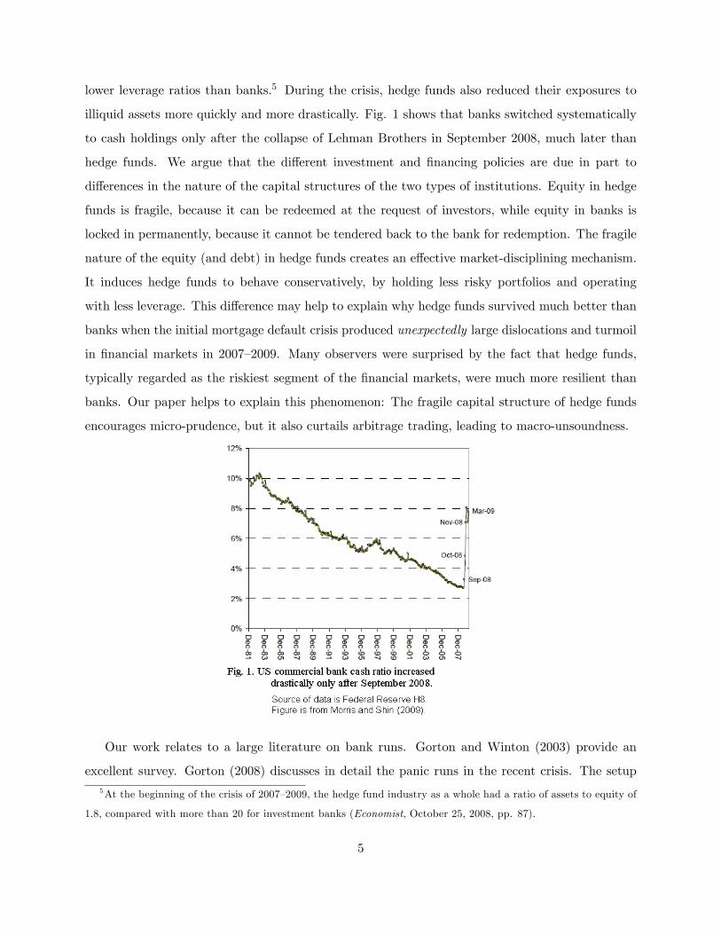
illiquid assets more quickly and more drastically. Fig. 1 shows that banks switched systematically

to cash holdings only after the collapse of Lehman Brothers in September 2008, much later than

hedge funds. We argue that the di¤erent investment and �nancing policies are due in part to

di¤erences in the nature of the capital structures of the two types of institutions. Equity in hedge

funds is fragile, because it can be redeemed at the request of investors, while equity in banks is

locked in permanently, because it cannot be tendered back to the bank for redemption. The fragile

nature of the equity (and debt) in hedge funds creates an e¤ective market-disciplining mechanism.

It induces hedge funds to behave conservatively, by holding less risky portfolios and operating

with less leverage. This di¤erence may help to explain why hedge funds survived much better than

banks when the initial mortgage default crisis produced unexpectedly large dislocations and turmoil

in �nancial markets in 2007�2009. Many observers were surprised by the fact that hedge funds,

typically regarded as the riskiest segment of the �nancial markets, were much more resilient than

banks. Our paper helps to explain this phenomenon: The fragile capital structure of hedge funds

encourages micro-prudence, but it also curtails arbitrage trading, leading to macro-unsoundness.

Our work relates to a large literature on bank runs. Gorton and Winton (2003) provide an

excellent survey. Gorton (2008) discusses in detail the panic runs in the recent crisis. The setup5At the beginning of the crisis of 2007�2009, the hedge fund industry as a whole had a ratio of assets to equity of

1.8, compared with more than 20 for investment banks (Economist, October 25, 2008, pp. 87).

5

in our model is similar to that in Diamond and Dybvig (1983). The di¤erence is that we assume

that the size of early withdrawals is ex ante random, and this allows us to study the optimal cash

holding problem of a hedge fund. In general, a bank-run game has multiple equilibria, but we

resort to global game methods to solve for the unique equilibrium. In this respect, our paper is

close to the work of Goldstein and Pauzner (2005), but the purpose and the scope of the two papers

di¤er.6 We study the optimal cash holdings in the balance sheets of hedge funds, while Goldstein

and Pauzner study the optimal liquidity provision of banks.

A panic run can be driven by liquidity concerns or by concerns about solvency (see the discussion

in Brunnermeier, 2009). In our model, the realization of large early withdrawals forces a hedge

fund to liquidate positions in illiquid markets at reduced prices, and this triggers a run. In contrast,

the run can be driven by fundamentals, as in Goldstein and Pauzner (2005). Bad fundamentals

leave little asset value for investors who withdraw late, and this causes an immediate run. In the

recent �nancial crisis, capital markets experienced many runs triggered for liquidity reasons, rather

than for fundamental reasons. There were runs on many �nancial institutions that appeared to

have adequate regulatory capital before they collapsed. Even so, investors ran, worried that the

�nancial institutions had insu¢ cient liquidity to meet massive early withdrawals and that assets

would have to be liquidated at a deep discount.

Our work also relates to Chen, Goldstein, and Jiang (2010). They �nd that mutual fund

out�ows are signi�cantly more sensitive to poor performance for funds that invest in illiquid assets.

This insight is similar to our result that market illiquidity potentially generates a panic run on

high-end �nancial intermediaries, such as hedge funds and mutual funds. Compared with their

work, we explicitly model how hedge fund managers factor into their ex ante investment and

�nancing decisions the ex post panic run. In the same vein as Shleifer and Vishny (1997), Stein

(2005) argues that open-ended funds, as a result of competition, could be suboptimal, because their

investments are limited by the occurrence of early withdrawals in response to poor performance.

Our emphasis is on the mechanisms that curtail arbitrage. Our focus on coordination risk di¤ers

6The global game methodology has been used in various contexts. For example, Rochet and Vives (2004) also use

global games to study bank runs. Other applications include currency crises (Morris and Shin, 1998; and Corsetti,

Dasgupta, Morris, and Shin, 2004), contagion of �nancial crises (Dasgupta, 2004; and Goldstein and Pauzner, 2004),

and market liquidity (Morris and Shin, 2004; Plantin, 2009; and Plantin, Sapra, and Shin, 2008).

6

from the arguments presented in these papers. In a banking context, Morris and Shin (2008) also

argue that cash held by a debtor bank can lower the threshold of coordination among creditors to

not withdraw. They do not formalize the argument, however, which we develop further by studying

the ex ante optimal asset allocation decision of hedge funds and the limits to arbitrage.

The paper is organized as follows. In Section 2, we �rst describe the model setup. Next, we solve

the optimal asset allocation for a hedge fund, without and with the coordination problem facing

the fund�s investors. After that we analyze the model�s implications and predictions. In Section

3, we generalize the model and discuss some broader issues of relevance to �nancial markets. In

Section 4, we provide remarks and conclusions.

2 The model

We present the model in this section.

2.1 The setup

We use a model with four dates: T0, T 12, T1, and T2. All agents are risk-neutral. There is no

discount factor between T1 and T2:

2.1.1 Hedge fund

Consider a simple setup of a hedge fund that depends on investors for funding. The investors are

the limited partners of the fund. The fund begins at T0 and ends at T2. Investors have the right to

redeem their investments at an intermediate date, T1. We assume that the total amount of assets

managed by the fund at T0 is 1, that there is a continuum of investors with measure 1, and that each

investor contributes 1 unit of capital. We model the liquidity risk of the hedge fund�s liabilities

as follows: Each investor in the hedge fund is either an early investor or a late investor. Early

investors are investors who, despite initially having the intention of staying for a long time with the

fund, end up redeeming their investments at T1 for reasons that we leave unspeci�ed but that could

be related to consumption, portfolio allocation, or other �nancial emergencies. The probability

that an investor is an early investor, depending on the state of the economy, is ex ante a random

7

variable, uniformly distributed with support � 2 [0; �], where 0 < � < 1. Then, in aggregate, the

ex ante proportion of investors who end up as early investors is given by the random variable �.

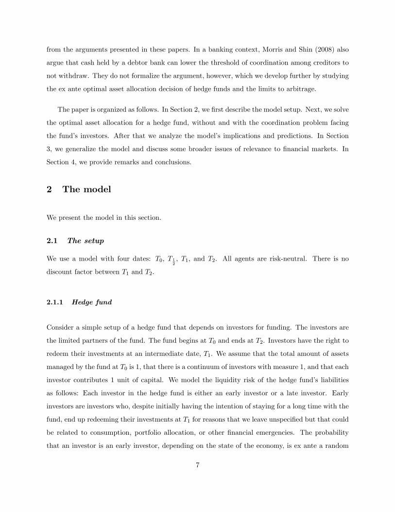
At T0, the hedge fund needs to make an asset allocation decision: How much capital X should

be invested in cash (C)? The remaining capital, 1 � X, is invested in illiquid assets (AL). The

cost of investment per unit of the illiquid assets at T0 is 1. We assume illiquid assets have a (gross)

return of R at T2, without any uncertainty, where R > 1. However, if illiquid assets are liquidated

early, at T1, they are sold at a discount, where the discounted price at �re sale is � (per unit), with

0 < � < 1. Fig. 2 shows the hedge fund�s balance sheet. Notice that there is no leverage, only

equity. We discuss a levered hedge fund later.

2.1.2 Investors

At T 12, uncertainty about the investors�status is resolved. At that time each investor knows whether

he is an early investor or not, but no investor knows the status of other investors. Nevertheless, late

investors receive signals about the state of the economy or the aggregate number of early investors

(�). More speci�cally, late investor i0s signal is �i = � + �i, where �i is a uniformly distributed

variable with support [��; �]. �i is independent from �j for i 6= j. In most of our analysis, " is

assumed to be arbitrarily small: � ! 0, which is a typical setup in applications of global games.

Further, at T 12, investors are perfectly informed about the cash position X as well as about the

market depth, �. The fund�s position in cash can be known either because the fund discloses this

in a regular letter to investors or because many investors in hedge funds are themselves professional

investors with access to the management of the fund. Usually, a hedge fund is very cautious about

8

disclosing trading strategies or positions in speci�c assets, but it does not object to disclosing

allocations in general asset classes.

At T 12, all investors need to decide whether to stay in the fund until T2 or to redeem their shares

at T1, in which case they inform the fund about their decisions. All early investors have to redeem.

A late investor might decide to redeem if he thinks that many other investors may redeem, because

too many withdrawals force the hedge fund to liquidate illiquid investments at a cost. It is the

coordination problem among late investors that we want to study in this paper.

Let us consider the payo¤s of an investor, whether an early or a late investor, from redemption

and nonredemption. Suppose that the aggregate number of investors that redeem at T1 is given by

s, where 0 � s � 1.

The payo¤ function of an investor that redeems is

wR(s) =

8<: 1 if 0 � s � X + (1�X)�X+(1�X)�

s if X + (1�X)� < s � 1(1)

Note that, in Eq. (1), investors withdrawing their shares at T1 receive a fraction of the hedge

fund�s net asset value. At T 12, when investors give the fund notice of their redemptions, the hedge

fund�s mark-to-market net asset value is 1, not the amount X+(1�X)� shown in Eq. (1). This is

because the hedge fund possesses cash reserves, and as long as it has not started to liquidate illiquid

assets, the mark-to-market value of the fund is 1.7 Investors that withdraw are paid based on a

proportion of this initial mark-to-market value of the fund, 1. However, if too many withdrawals

occur, the hedge fund must liquidate illiquid assets after it exhausts its cash balance, X. The

sale price of the illiquid assets is only �, less than 1. When this happens, the realized value of

an investor�s share of the assets is lower than his claim. To ful�ll early investors�claims, the fund

has to liquidate part of the late investors� shares of the assets. The fund might have to sell all

assets at T1, in which case late investors are left with nothing. This �rst-mover advantage of early

7We can assume that, when the hedge fund sells its illiquid assets, the fund faces a special downward-sloping

demand curve. Speci�cally, the market can absorb just a tiny amount of the assets at a price of 1. After absorbing

that amount, the price drops to � and the demand curve becomes perfectly elastic with constant price �. Therefore,

before the sale, the mark-to-market value of the fund is 1, but at liquidation it becomes X + (1�X)�.

9

withdrawals, due to discounted prices at �re sales and the �rst-come, �rst-served right to cash

�ows, is the fundamental reason for a run on hedge funds and on mutual funds (see the discussion

in Brunnermeier, 2009).

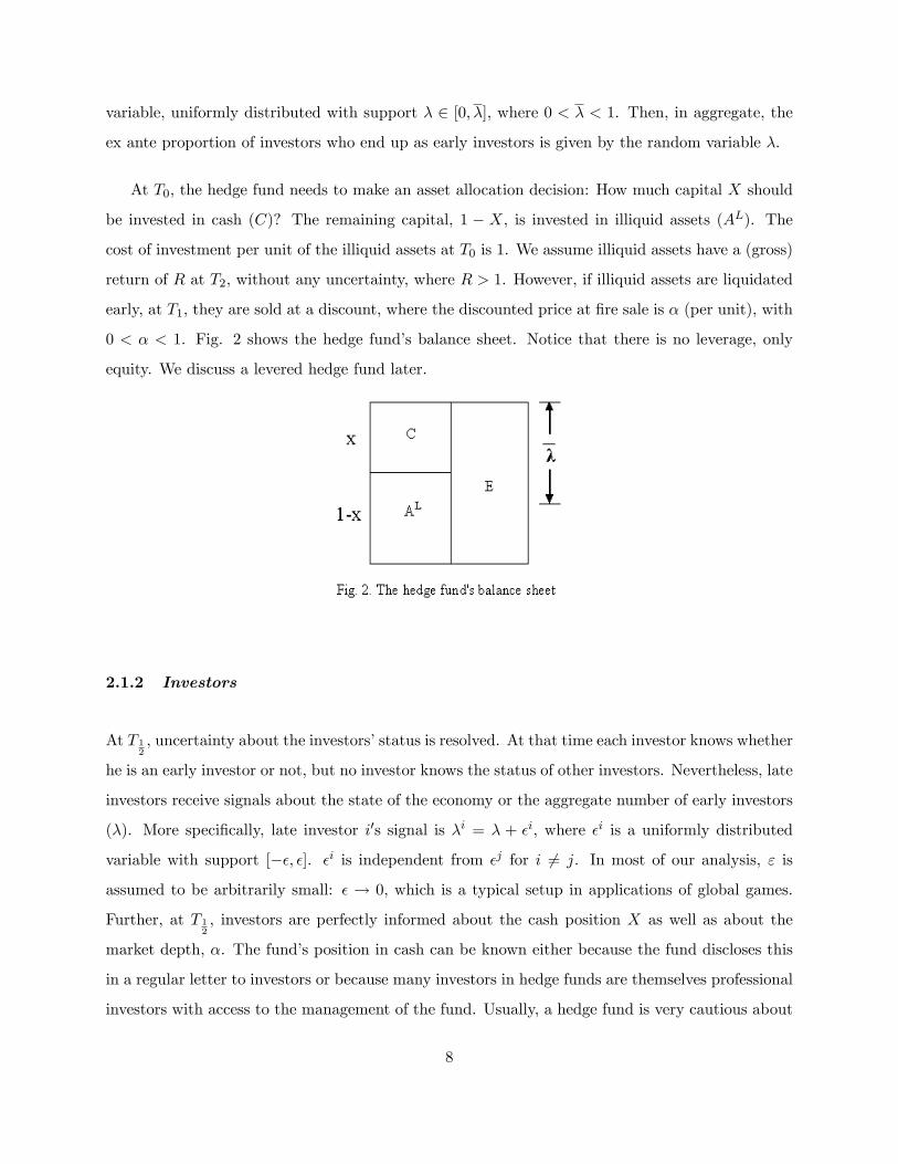
The payo¤ function of an investor that does not redeem at time T1 (but stays) is

wS(s) =

8>>><>>>:(X�s)+(1�X)R

1�s if 0 � s � X(1�X)� s�X

�1�s R if X < s � X + (1�X)�

0 if X + (1�X)� < s � 1

. (2)

In Eq. (2), when the aggregate number of investors that redeem at T1 is less than X, the

fund does not need to liquidate any long-term illiquid assets. Thus the value of the fund at T2 is

(X � s) + (1�X)R. However, if the aggregate number of investors withdrawing is higher than X,

the fund must sell some of its illiquid assets at T1. The number of units of the illiquid assets that

need to be sold is s�X� , where s � X is the amount of cash short to satisfy redemptions. If the

number of withdrawing investors exceeds the total liquidation value of the fund, X+(1�X)�, the

hedge fund is completely liquidated and nothing is left after T1, the third line in Eq. (2).

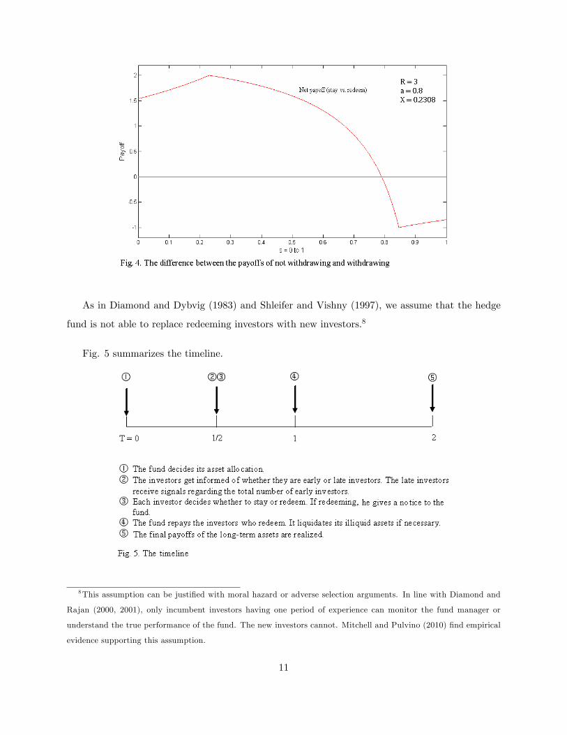
We de�ne the di¤erence between the payo¤s of not withdrawing at time T1 and withdrawing as

�w(s) � wS(s)� wR(s). Fig. 3 shows the payo¤s wS(s) and wR(s), and Fig. 4 shows �w(s).

10

As in Diamond and Dybvig (1983) and Shleifer and Vishny (1997), we assume that the hedge

fund is not able to replace redeeming investors with new investors.8

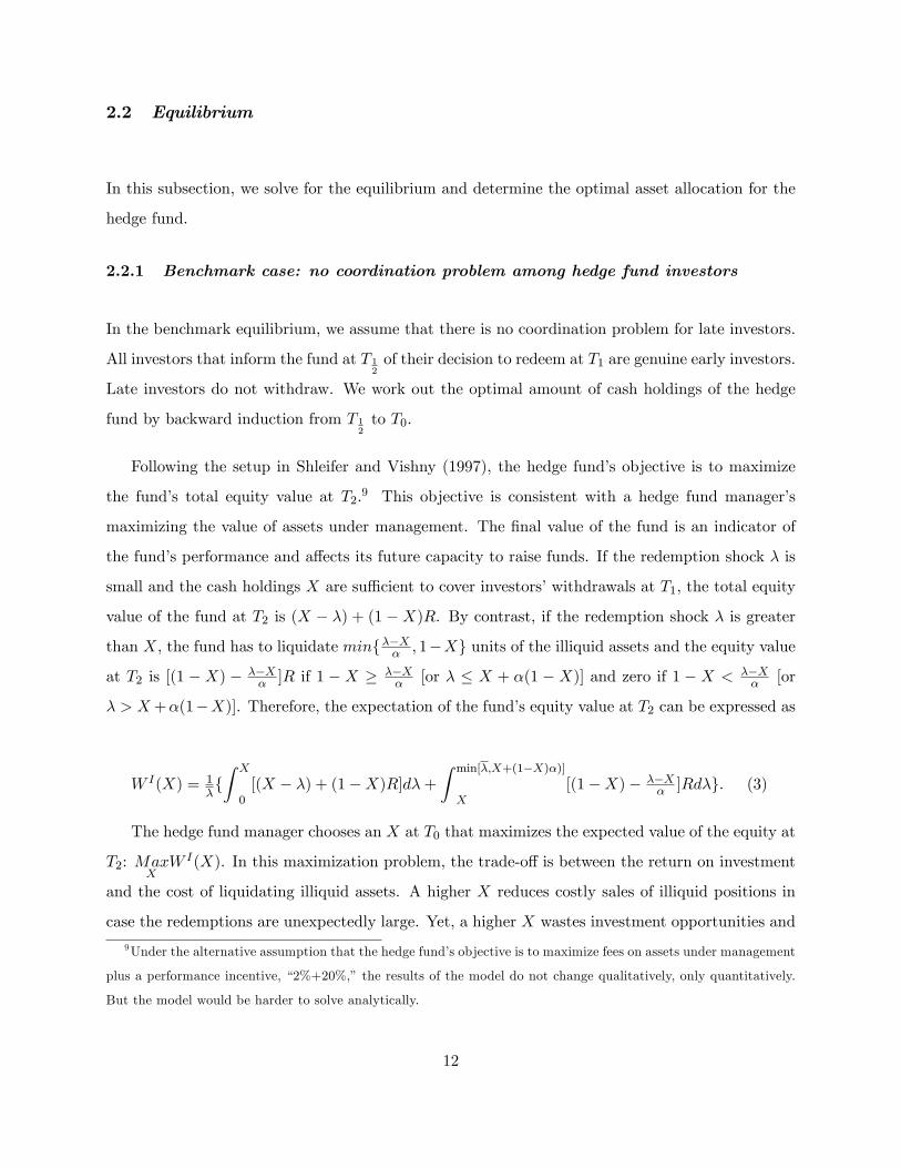
Fig. 5 summarizes the timeline.

8This assumption can be justi�ed with moral hazard or adverse selection arguments. In line with Diamond and

Rajan (2000, 2001), only incumbent investors having one period of experience can monitor the fund manager or

understand the true performance of the fund. The new investors cannot. Mitchell and Pulvino (2010) �nd empirical

evidence supporting this assumption.

11

2.2 Equilibrium

In this subsection, we solve for the equilibrium and determine the optimal asset allocation for the

hedge fund.

2.2.1 Benchmark case: no coordination problem among hedge fund investors

In the benchmark equilibrium, we assume that there is no coordination problem for late investors.

All investors that inform the fund at T 12of their decision to redeem at T1 are genuine early investors.

Late investors do not withdraw. We work out the optimal amount of cash holdings of the hedge

fund by backward induction from T 12to T0.

Following the setup in Shleifer and Vishny (1997), the hedge fund�s objective is to maximize

the fund�s total equity value at T2.9 This objective is consistent with a hedge fund manager�s

maximizing the value of assets under management. The �nal value of the fund is an indicator of

the fund�s performance and a¤ects its future capacity to raise funds. If the redemption shock � is

small and the cash holdings X are su¢ cient to cover investors�withdrawals at T1, the total equity

value of the fund at T2 is (X � �) + (1 �X)R. By contrast, if the redemption shock � is greater

than X, the fund has to liquidate minf��X� ; 1�Xg units of the illiquid assets and the equity value

at T2 is [(1 � X) � ��X� ]R if 1 � X � ��X

� [or � � X + �(1 � X)] and zero if 1 � X < ��X� [or

� > X+�(1�X)]. Therefore, the expectation of the fund�s equity value at T2 can be expressed as

W I(X) = 1�fZ X

0[(X � �) + (1�X)R]d�+

Z min[�;X+(1�X)�)]

X[(1�X)� ��X

� ]Rd�g. (3)

The hedge fund manager chooses an X at T0 that maximizes the expected value of the equity at

T2: MaxXW I(X). In this maximization problem, the trade-o¤ is between the return on investment

and the cost of liquidating illiquid assets. A higher X reduces costly sales of illiquid positions in

case the redemptions are unexpectedly large. Yet, a higher X wastes investment opportunities and

9Under the alternative assumption that the hedge fund�s objective is to maximize fees on assets under management

plus a performance incentive, �2%+20%,� the results of the model do not change qualitatively, only quantitatively.

But the model would be harder to solve analytically.

12

forgoes the high return R in case the redemption shock is small. The trade-o¤ leads to a unique

optimal value for the cash holdings, X�.

Theorem 1 If 0 < � � R��R(2��)�1 , the optimal amount of cash holdings is X

� = R�R�R�� �. The fund

survives any redemption shock � 2 [0; �], where � � X� + (1 � X�)�. If R��R(2��)�1 < � < 1, the

optimal amount of cash holdings is X� = R(1��)R(2��)�1 . The fund survives if the redemption shock lies

within � 2 [0; X� + (1�X�)�] � [0; �], where X� + (1�X�)� < �.

Proof: See the Appendix.

2.2.2 Equilibrium when there is a coordination problem among hedge fund investors

When the cash holdings, X, do not exceed the realized redemption shock, �, a costly sale of illiquid

assets is unavoidable. The �re sale depresses the fund�s net asset value and potentially causes a

run by investors. The fund manager anticipates this possibility of a run and rationally takes it into

account when deciding the fund�s cash balances.

Again, we solve the equilibrium by backward induction, from T 12to T0. In the �rst step, we

work out investors�decisions at T 12for a given cash balance X. In the second step, we go back to

T0 and solve for the fund�s optimal cash holdings X by taking into account the investors�responses.

2.2.2.1. Investors�decision at T 12given the cash holdings X

At T 12, late investor i�s decision rule can be characterized as a map: (�i, X) 7�! (Withdraw,

Stay), where (�i, X) is the information set of investor i and (Withdraw, Stay) is his choice set.

We need to work out investors�decision rules that form an equilibrium. We �rst examine late

investors�strategies when the state of economy � is extremely low or extremely high. We have the

following two extreme cases.

First, there exists a lower dominance region of � 2 [0; �L), in which staying in the fund is the

dominant strategy for late investors. To obtain the lower dominance region in the bank-run game,

we follow Goldstein and Pauzner (2005) and modify the technology for a very low �. Speci�cally, we

13

assume that when the proportion of early investors (the state of the economy) � falls within [0; �L)

(where �L is close to zero), there is no discount in the sale price of the illiquid assets, i.e., � = 1.10

With this modi�cation, we can conclude that if a late investor knows that � is in the region [0; �L),

he does not run, no matter his beliefs about other investors�actions. This is because if there is

no discount, early withdrawals do not erode the late investors�shares. Thus, late investors do not

su¤er any disadvantage if they wait until T2 to withdraw. In most of our analysis, " is taken to

be arbitrarily close to zero, so late investors are sure that � is in [0; �L). Staying is therefore their

dominant strategy.

Second, using the result that s� = X + (1 �X)�(R�1)R�� solves the equation wS(s) = wR(s), we

de�ne �U � s�. Then, an upper dominance region of � 2 (�U ; �] exists, in which withdrawing

is the dominant strategy for late investors. The reason is as follows: When � > �U , there are a

su¢ cient number of redemptions by early investors, and, consequently, even if all late investors

choose to stay, the payo¤ of a late investor if he decides to redeem early is higher than the payo¤

if he decides to stay on. If a late investor is sure that � > �U , he should redeem no matter his

beliefs about the actions of other late investors. As " is taken to be arbitrarily close to zero, late

investors are informed when � > �U . Therefore, if � is in the interval (�U ; �], withdrawing is the

dominant strategy for late investors. In our model, we show that it is not optimal for the hedge

fund to choose cash holdings X such that X+(1�X)�(R�1)R�� � �. Therefore, the condition � > �U

is always true in our model. That is, the upper dominance region (�U ; �] exists.

For the intermediate region of � 2 [�L; �U ], late investors�decisions depend on their beliefs about

the actions of other late investors. The signals regarding � form their beliefs. Our main interest is

in the threshold-strategy equilibrium in which a late investor�s strategy depends on the signal he re-

ceives. Speci�cally, the threshold-strategy equilibrium is the equilibrium in which every late investor

sets a threshold ��(X) and uses the threshold strategy (�i, X)7�!

8<: Withdraw �i > ��(X)

Stay �i � ��(X), such

10Using � to represent the state of the economy has the following meaning: A low � indicates that few investors are

in need of withdrawing (funding liquidity) because the economy is doing well. Presumably, these are also times when

the level of market liquidity is high and � is consequently high. Implicitly, we are assuming that funding liquidity and

market liquidity are positively correlated when the state of the economy is bad. This is consistent with the empirical

evidence.

14

that, given that all other late investors set the threshold as ��(X), it is optimal for a particular

late investor to do that. We prove that there is a unique threshold equilibrium for our model.

We use global game methods to solve for the unique threshold equilibrium. Note that we do

not consider equilibria other than the threshold strategy in this paper. With the assumptions made

before about the existence of the two extreme dominance regions of �, it is possible to provide a

proof, as in Goldstein and Pauzner (2005), that the threshold equilibrium is the only equilibrium.11

The equilibrium result is summarized in Theorem 2.

Theorem 2 The model has a unique threshold equilibrium. In the equilibrium, a late investor

redeems if, and only if, his signal is above the threshold ��(X).

We prove the theorem in several steps.

First, suppose that every late investor uses the threshold strategy and sets the threshold as

��(X). We want to determine the total number of investors (both early and late investors) that

decide to redeem at T1 for a given realization of �. Given the realized � and the threshold ��, the

proportion of late investors that run equals �+����

2� . Hence, the total number of investors redeeming,

denoted by s(�, ��(X)), is

s(�, ��(X)) =

8>>><>>>:� if � � ��(X)� �

�+ (1� �)�+����(X)

2� if ��(X)� � � � � ��(X) + �

1 if � � ��(X) + �

. (4)

When �� � � � � � �� + �, s(�, ��(X)) has two components. The �rst component represents

redemptions by early investors, and the second one represents redemptions by some late investors

who change their minds and decide instead to redeem early.

Second, after the late investor receives the signal �i his posterior distribution of � is uniform in

the interval [�i��; �i+�]. Therefore, the investor�s expected net payo¤ of staying versus redeeming

is11 In fact, it has become a standard result in the global game literature [see Morris and Shin (2003) for a discussion

of Goldstein and Pauzner�s result] that the threshold equilibrium is the only equilibrium for a bank-run game as long

as the noise of the signal is uniformly distributed.

15

�(�i; ��) = 12�

Z �i+�

�i���w(s(�; ��))d�. (5)

Third, the marginal late investor who receives the threshold signal �� is indi¤erent between

redeeming and staying. Therefore, �(��; ��) = 0. That is,

12�

Z ��+�

�����w(s(�; ��))d� = 0. (6)

As previously pointed out, in our model we focus on the case of an arbitrarily small �: � ! 0.

This assumption makes the model tractable and helps to highlight the main insights of the paper.

When � ! 0, fundamental uncertainty disappears, while strategic uncertainty remains unchanged

(see Morris and Shin, 1998). In our context, from the marginal late investor�s perspective, � falls

within [�� � �; �� + �]. When � ! 0, the uncertainty associated with the �rst element of s(�; ��)

disappears while the uncertainty related to the second element does not. As a whole, s(�; ��) is

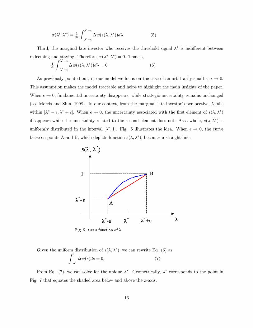
uniformly distributed in the interval [��; 1]. Fig. 6 illustrates the idea. When � ! 0, the curve

between points A and B, which depicts function s(�; ��), becomes a straight line.

Given the uniform distribution of s(�; ��), we can rewrite Eq. (6) asZ 1

���w(s)ds = 0. (7)

From Eq. (7), we can solve for the unique ��. Geometrically, �� corresponds to the point in

Fig. 7 that equates the shaded area below and above the x-axis.

16

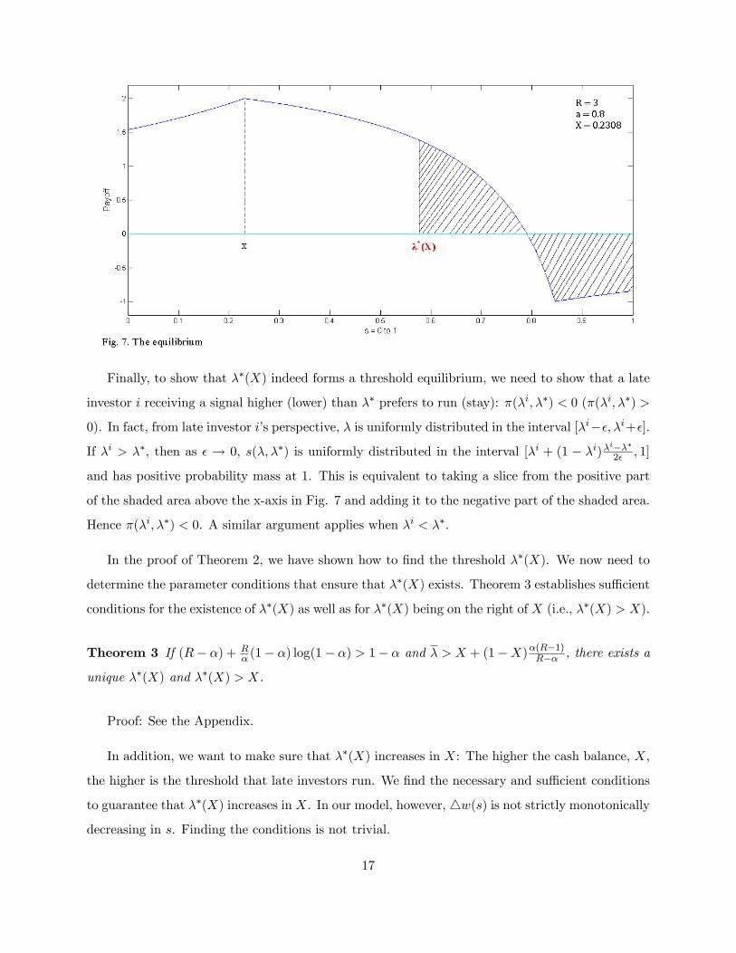
Finally, to show that ��(X) indeed forms a threshold equilibrium, we need to show that a late

investor i receiving a signal higher (lower) than �� prefers to run (stay): �(�i; ��) < 0 (�(�i; ��) >

0). In fact, from late investor i�s perspective, � is uniformly distributed in the interval [�i��; �i+�].

If �i > ��, then as � ! 0, s(�; ��) is uniformly distributed in the interval [�i + (1 � �i)�i���2� ; 1]

and has positive probability mass at 1. This is equivalent to taking a slice from the positive part

of the shaded area above the x-axis in Fig. 7 and adding it to the negative part of the shaded area.

Hence �(�i; ��) < 0. A similar argument applies when �i < ��.

In the proof of Theorem 2, we have shown how to �nd the threshold ��(X). We now need to

determine the parameter conditions that ensure that ��(X) exists. Theorem 3 establishes su¢ cient

conditions for the existence of ��(X) as well as for ��(X) being on the right of X (i.e., ��(X) > X).

Theorem 3 If (R� �) + R� (1� �) log(1� �) > 1� � and � > X + (1�X)

�(R�1)R�� , there exists a

unique ��(X) and ��(X) > X.

Proof: See the Appendix.

In addition, we want to make sure that ��(X) increases in X: The higher the cash balance, X,

the higher is the threshold that late investors run. We �nd the necessary and su¢ cient conditions

to guarantee that ��(X) increases in X. In our model, however, 4w(s) is not strictly monotonically

decreasing in s. Finding the conditions is not trivial.

17

Theorem 4 ��(X) is an increasing function with respect to X when R� log(

1��1�b ) < log� (where b

solves (R� � 1)(�� b) +R� (1� �) log(

1��1�b ) = �� log�).

12

Proof: See the Appendix.

As we have obtained the unique threshold and because �! 0 , we conclude that all late investors

run if � > ��(X) and none runs if � � ��(X). Therefore, the total number of investors redeeming

their investments from the hedge fund can be expressed as

s(�) =

8<: � if � � ��(X)

1 if � > ��(X). (8)

2.2.2.2. The fund�s optimal cash holding decision at T0

We now go back to T0 and look at the hedge fund�s optimal cash holding decision when a run by

investors might occur. To save space and simplify the analysis, we focus on the case � > R��R(2��)�1 .

For the case � � R��R(2��)�1 , the main results do not change.

13

We analyze two regions of X, in order: X 2 fX jX + (1 � X)�(R�1)R�� < �g and X 2 fX

jX + (1 �X)�(R�1)R�� � �g. In the �rst region, X is low and the only equilibrium is the threshold

equilibrium. In the second region of X, we make a weak assumption that investors coordinate and

choose the Pareto e¢ cient equilibrium� the staying-strategy equilibrium. That is, late investors

ignore the signals received and stay: (�i, X)7�!Stay.14

12The parameter conditions in Theorems 3 and 4 are not restrictive at all. A wide set of parameters achieves the

results. In fact, the reason for requiring parameter conditions is that a bank-run game does not have strictly global

strategic complementarities, i.e., in our model, 4w(s) is not strictly monotonically decreasing in s. However, in Fig.

7, we see the intuition for why the parameter conditions are not restrictive: Toward the end of s = 1, 4w(s) does

not decrease but increases very slowly.13 In fact, we can assume that � must satisfy � > R��

R(2��)�1 . That is, we can assume that only these are the

parameter values that are relevant in this research. But it is easy to prove that the conclusions in this subsection

are true in the alternative case of �. The economic idea of the proof is exactly the same. Only the mathematical

technique changes.14 If investors still use the threshold equilibrium for the second region of X, the model result is strengthened,

because we do not need to consider the second region of X separately.

18

We begin the analysis from the low region ofX, i.e., X 2 [0; XC), whereXC+(1�XC)��(R�1)R�� =

�. In this region of X, investors use the threshold strategy in equilibrium. Because investors use the

threshold strategy and set the threshold as ��(X), the fund knows that if the realized redemption

shock is greater than ��(X), all investors redeem and desert the fund, driving its net asset value

to zero. The fund survives if � 2 [0; ��(X)].15

The expected value of the fund is

W II(X) = 1�fZ X

0[(X ��)+ (1�X)R]d�+

Z ��(X)

X[(1�X)� ��X

� ]Rd�g for X 2 [0; XC). (9)

BecauseW II(X) is a continuous and bounded function with respect toX in the support [0; XC),

the problem MaxXW II(X) has a solution.16 The �rst-order condition of Eq. (9) is

[(1� R� )X + 1��

� ��(X)R] + [(X + (1�X)�� ��(X)] � R� �d��(X)dX = 0. (10)

The trade-o¤ in Eq. (10) is as follows. The �rst term on the left-hand side is the e¤ect of a

higher X on the value of the fund, given the survival range [0; ��(X)]. This term captures the

trade-o¤ when there is no run. The trade-o¤ is between higher returns (R) by investing more in

illiquid assets and a lower cost of liquidation by holding more cash. This trade-o¤ was examined

when we studied the benchmark equilibrium. As X increases, the �rst term becomes negative.

Mathematically, this is because ��(X) increases at a lower rate than X. The economic intuition is

that if X is too high, it distorts the optimal trade-o¤ examined in the benchmark equilibrium. The

second term in Eq. (10) is new. It represents the e¤ect on the value of the fund from increasing

the survival window. This term is always positive: Increasing the amount of cash X in the fund

increases the survival range [0; ��(X)]. Overall, the sum of the two terms equals zero for some

interior X. We denote this unique interior solution as X��.

Theorem 5 There exists a unique optimal amount of cash holdings in the hedge fund�s balance

sheet, X��, in the interval (0; XC) that maximizes the hedge fund value W II(X).

15By the properties of ��(X), the inequality ��(X) < X + (1 � X)�(R�1)R�� < � is valid and, therefore, the upper

limit of the survival window is min[��(X); X + (1�X)�; �] = ��(X).16Rigorously, Max

XW II(X) can be written as Sup

XW II(X).

19

Proof: See the Appendix.

Next, we analyze the second region of X, where X 2 [XC ; 1]. In this region, cash holdings are

very high, and all late investors decide to stay with the fund. The expected value of the fund is,

therefore, equal to that in the benchmark case:

W II(X) =W I(X) = 1�fZ X

0[(X��)+(1�X)R]d�+

Z �

X[(1�X)� ��X

� ]Rd�g forX 2 [XC ; 1].17

(11)

Because � > R��R(2��)�1 , using the proof of Theorem 1, it is easy to show that W II(X) is

decreasing in the interval X 2 [XC ; 1]. Therefore, W II(X) achieves a maximum at X = XC . We

need to prove that this maximum value is less than that in the region X 2 [0; XC ], or W II(XC) <

W II(X��). This is true under general parameter values. Therefore, it is too costly for the hedge

fund to choose cash holdings in the second region.

Theorem 6 For general parameter values, we have that W II(XC) < W II(X��).18 That is, it is

not optimal for the hedge fund to hold cash in the interval X 2 [XC ; 1]. Globally, the optimal

amount of cash holdings is X��.

Proof: See the Appendix.

The intuition for Theorem 6 is simple. A fund that holds a large amount of cash is better

able to persuade late investors to stay on, eliminating the coordination problem and increasing its

chances of survival. This policy is too costly, though, because the fund forgoes valuable investment

opportunities. It is better that the fund holds less cash. Globally, the optimal amount of cash

holdings is still X��, which lies in the �rst region.

We wish to prove that the optimal amount of cash when a run is possible is higher than the

optimal amount of cash when there is no risk of a run, i.e., X�� > X�.

17Because X + (1�X)�(R�1)R�� > �, the upper limit of the fund�s survival window is min[�;X + (1�X)�)] = �.

18The need for parameter assumptions here is because we made a weak assumption; that is, investors coordinate

and choose the staying-strategy equilibrium for the second region of X. If investors continue to use the threshold

equilibrium, Theorem 6 is true automatically and does not require any parameter assumptions.

20

We look at what happens if the fund keeps the original cash holdingsX�. Because � > R��R(2��)�1 ,

from Theorem 1, X� + (1�X�)� < �. Because X� + (1�X�)�(R�1)R�� < X� + (1�X�)�, we have

that X� + (1 � X�)�(R�1)R�� < �. Therefore, we conclude that X� indeed lies in the �rst region.

Furthermore, by the properties of ��(X), we have that ��(X�) < X� + (1 � X�)�. That is, the

e¤ect of the run causes the survival range to shrink from [0; X� + (1�X�)�] to [0; ��(X�)].

Because an increase in X widens the survival range [i.e., ��(X) increases in X], the hedge fund

may need to increase the optimal X� in the benchmark equilibrium to achieve a wider survival

range and thus maximize the fund value. We evaluate the �rst-order derivative of W II(X) at

X = X� to check the change in W II(X) when X is changed:

dW II(X)dX j

X=X� = [(1� R� )X +

1��� ��(X)R]j

X=X� + f[(X +(1�X)����(X)] � R� �

d��(X)dx gj

X=X� .

(12)

An increase in X at X = X� has two e¤ects on W II(X). The second term in Eq. (12), the

dominant e¤ect, is positive. It captures the gains from increasing the survival range. The �rst term

of Eq. (12) is negative. The intuition for the �rst term is as follows. At the e¤ective maximum

shock, X� + (1�X�)�, the optimal amount of cash is X�. Because the e¤ective maximum shock

decreases to ��(X�), the optimal cash holdings should be lower. However, this e¤ect is second order

compared with the �rst e¤ect under general parameter values. That is, overall, dWII(X)dX j

X=X� > 0,

meaning that the fund can increase its value at T2 by increasing its positions in cash.

Theorem 7 For general parameter values, we have that X�� > X�.19 That is, the optimal amount

of cash holdings when a run is possible is higher than when a run is not taken into account.

Proof: See the Appendix.

Theorem 7 is a key result of the paper. It shows how runs on hedge funds a¤ect hedge funds�

optimal cash holdings. It is important to emphasize that ex post runs impact the optimal amount

19The need for parameter assumptions is purely for technical reasons. In fact, the �rst term in Eq. (12) is negative

due to � ! 0. In general cases, when � is not arbitrarily small, the �rst term is also positive. Thus, the inequality

that dW II (X)dX

jX=X� > 0 is always true; it does not depend on particular parameter values. That is, X�� > X� holds

in general if we do not focus on �! 0.

21

of cash ex ante in two ways. The �rst one is the response e¤ect, represented by the �rst term on

the left-hand side of Eq. (10). Because of the risk of a run, redemptions include not only early

investors but also some late investors. The size of total redemptions is thus changed because of

runs. In response to an increase in the size of redemptions, the hedge fund manager adjusts the

optimal cash holdings upward. The second channel is the signaling e¤ect and is captured by the

second term on the left-hand side of Eq. (10). The probability of the run and, hence, the size of

total redemptions is a function of the hedge fund�s cash holdings. The fund manager holds more

cash to �signal�and reassure investors, and thus to reduce the likelihood of a run.

Before closing this subsection, we illustrate the results of the model with a numerical example.

We set the parameter values to R = 3; � = 0:8, and � = 0:9. With these values, the optimal

amount of cash holdings without considering a run is X� = 0:23. The hedge fund survives as long

as � 2 [0; X� + (1 � X�)�] = [0; 0:85] � [0; 0:9]. With the cash holdings of X� = 0:23, however,

the e¤ect of a run reduces the fund�s survival range to � 2 [0; ��(X�)] = [0; 0:59]. The fund value

is W II(X�) = 1:27. Therefore, when a run is possible, it is optimal to increase the amount of

cash holdings as this increases the range of values of � at which the fund survives. In fact, at

X� = 0:23, the survival range of the fund changes at a rate of d��(X)dX j

X=X� = 0:52, and the value of

the fund changes at a rate dW I(X)dX j

X=X� = 0:31. Therefore, the value of the fund can be increased

by increasing the amount of cash holdings, X.

Indeed, if the cash holdings are increased to X�� = 0:34, the survival range widens to � 2

[0; ��(X��)] = [0; 0:64]. We have d��(X)dX j

X=X�� = 0:53 anddW II(X)dX j

X=X�� = 0. Therefore, the fund

achieves its highest expected value at X = X��, where W II(X��) = 1:30. Note that X + (1 �

X)�(R�1)R�� jX=X�� = 0:82 < � is true.

If the fund increases the cash holdings to XC = 0:63, there is no coordination problem among

investors. This provides the widest survival range of the fund, � 2 [0; �] = [0; 0:9]. But this policy

is too costly and, therefore, it is not optimal. In fact, the maximum value of the fund within the

region X 2 [XC ; 1] is W II(XC) = 1:18, which is less than W II(X��) = 1:30.

Fig. 8 depicts how W I(X) and W II(X) change with X. W I(X) is above W II(X), meaning

that a run causes the value of the fund to go down. W I(X) achieves its highest value at X = 0:23,

whileW II(X) has a positive slope at X = 0:23 and achieves a maximum at X = 0:34. For values of

22

X above 0:63, there is no coordination problem any longer, and consequently W I(X) and W II(X)

coincide. The optimal cash holdings without considering a run are X� = 0:23 and the optimal cash

holdings when a run is possible are X�� = 0:34.

2.3 Implications and predictions of the model

In this subsection, we conduct a comparative statics analysis and study the model�s implications

and predictions.

2.3.1 Implications of the model

From Theorem 7, a panic run forces a hedge fund to hold excess cash. This shows that coordination

problems among investors induce a hedge fund to limit its exposure to illiquid assets.

Alternatively, the argument can be presented in the following way: Suppose that the reservation

utility (opportunity cost) of the hedge fund manager is C. That is, only if the expected value of

the fund at T2 is higher than C is the fund manager willing to participate in the market at T0.

We can prove that W I(X�; R) and W II(X��; R) are both increasing functions in the return, R.

Because W I(X�; R) > W II(X��; R), there exists an R� and an R�� such that W I(X�; R�) = C

and W II(X��; R��) = C, with R� < R��. Therefore, for returns R such that R� < R < R��,

23

coordination problems prevent the hedge fund manager from taking pro�table opportunities in

illiquid positions. These lost opportunities in the interval [R�; R��] represent limits to arbitrage.

Theorem 8 The coordination risk leads hedge funds to give up participating in the market when

the return R is moderately high (i.e., R� < R < R��).

Proof: See the Appendix.

In Theorem 8, missing arbitrage opportunities (R� < R < R��) occur not for the reason

presented in Shleifer and Vishny (1997), but because of the coordination risk and the potential

panic run on the hedge fund. Note that arbitrage opportunities are not taken only when returns

are moderately high. When returns are very high, hedge funds still take arbitrage positions. In

this sense, arbitrage activities are �limited�, not suspended completely, a result consistent with the

empirical evidence.

Research by Mitchell and Pulvino (2011) and Krishnamurthy (2010) provides convincing evi-

dence that, during the recent crisis, there were signi�cant arbitrage opportunities in debt markets.

Remarkably, Mitchell and Pulvino (2011) show that in many instances arbitrage failed because of

hedge funds�funding problems, instead of from problems related to the quality of the assets.

2.3.2 Predictions of the (ex post) probability of a run (at T1)

In our model, there are two factors that drive the probability of a run: � and �. From Eq. (8), we

can derive the ex post probability of a run Pr =

8<: 0 if � � ��(X)

1 if � > ��(X).20 It is easy to show that

@��(X)@� > 0. Therefore, @ Pr@� � 0 and @ Pr

@� � 0.

In our model, � is the proportion of investors facing �nancial constraints, i.e., needing to

withdraw money to cover for consumption, portfolio allocation, or other �nancial emergencies.

Essentially, we interpret � as the funding liquidity of hedge funds, i.e., the number of investors who

are in need of withdrawing early to cover their own liquidity shocks. Further, a fall in �, a sudden

drying up of market liquidity, also increases the probability of a run.21

20Due to �! 0, the function Pr is discrete. In general, Pr is continuous.21See Brunnermeier and Pedersen (2009) for more discussions about market liquidity and funding liquidity.

24

We o¤er Prediction 1.

Prediction 1: Runs on hedge funds are more likely to occur either under poor market liquidity

conditions or when large negative funding-liquidity shocks occur (i.e., a high �).

The impact of market liquidity is particularly relevant during a crisis, because markets typically

become illiquid, often systemically across di¤erent asset classes.

2.3.3 Predictions of the (ex ante) optimal cash holdings

Using Eq. (8), we can derive the ex ante probability of a run: Pr = 1 � ��(X)

�. We have that

@Pr@�> 0 and that @Pr@� < 0. Thus, we have a time series prediction for hedge funds�cash holdings.

Prediction 2 (time series of cash holdings): Hedge funds increase their cash holdings

when they expect either market liquidity or funding liquidity to worsen.

Also, because @Pr@� < 0, we have a cross-sectional prediction.

Prediction 3 (cross section of cash holdings): Hedge funds that invest more in illiquid

assets, and are consequently more likely to incur runs, are more likely to hold larger cash positions

as a precaution.

3 Discussion

So far we have assumed that the entire capital of hedge funds comes from their investor-clients

(equityholders), i.e., that funds carry no debt. While this is a gross simpli�cation, it allows us to

emphasize that the equity in hedge funds is fragile and subject to panic runs. This feature of hedge

funds distinguishes them from investment banks and commercial banks, where a panic run cannot

happen to the equity. In fact, equityholders of a bank cannot tender shares back to the bank for

redemption but can only trade ownership in the secondary market.

In addition to equity, hedge funds use leverage, most of it provided by their prime-brokers.

The debt of hedge funds is certainly susceptible to runs such as margin calls or sudden increases

25

in haircuts. Therefore, the whole right-hand side of the balance sheet of hedge funds is subject

to runs. In particular, hedge fund runs triggered by debtholders or by equityholders can reinforce

each other. Prime brokers calling the debt extended to a fund can scare the clients of the fund

and trigger redemptions. The opposite is also true: A drop in the assets under management due

to large scale redemptions induces prime brokers to impose stricter limits on leverage and reduce

credit.

These arguments imply that hedge funds seem to have little or no capital in a strict sense,

when capital is de�ned as �a long-term claim without a �rst-come-�rst-served right to cash �ows�

(see Diamond and Rajan, 2000). In other words, hedge funds have no real capital cushion on

their balance sheets that can be used to mitigate a panic run by debtholders or equityholders. In

contrast, banks have a capital cushion that can withstand the �rst loss if some debtholders start a

run.

We argue that the fragile nature of the capital structure of hedge funds has critical implications

both for individual hedge fund behavior and for capital markets.

3.1 Capital fragility encourages micro-prudence

Calomiris and Kahn (1991) and Diamond and Rajan (2001) argue that the coordination problem

inherent in a bank run works as a commitment device, since the bank can commit not to engage in

actions that dissipate value. Diamond and Rajan (2000) develop the argument further by adding

that bank capital requirements sometimes can be harmful and reduce welfare, since they weaken

the management�s commitment to behave appropriately by making the bank�s capital structure

less fragile.

In the same spirit, we argue that hedge funds, with more fragile capital structures than banks,

should be subject to greater market discipline. Tougher market discipline should lead to greater

care in both investment and �nancing decisions.22

With respect to investment decisions, our paper formally shows that hedge funds optimally

choose to hold more cash when a run is possible. Building on this logic, we expect that if a fund

22This conclusion is even stronger given that banks are protected by deposit insurance and hedge funds are not.

26

has some locked-up capital (i.e., some clients�funds are locked up until T2 and cannot be redeemed

earlier), then the fund holds less cash and invests more in illiquid assets. To prove this formally, we

adjust the original setup and assume that there is a tiny proportion (�) of investors that is locked

up. The proportion of investors that can run is thus 1 � � � �. We prove that the run threshold

increases and, hence, that the optimal cash holdings decrease.

Theorem 9 If the capital that is locked up is positive, i.e., � > 0, then the optimal amount of cash

holdings, X��, decreases (relative to when there is no capital that is locked up).

Proof: See the Appendix.

Theorem 9 sheds some light on why hedge funds, with little or no locked-up capital, are less

aggressive in trading illiquid assets than banks. The evidence shows that, as the recent crisis

unfolded, hedge funds rebalanced their portfolios toward cash holdings more aggressively and faster

than banks.

With respect to �nancing decisions, we can show that equity fragility makes hedge funds less

aggressive than banks in the use of leverage, as long as the market is not perfectly liquid, i.e.,

� < 1. The idea is as follows. Any rollover problem in hedge funds�short-term debt can ignite

a run not only by other debtholders but also by equityholders. Equityholders of banks, however,

cannot run. A rollover problem by some lenders of a bank can trigger a run by other lenders but

not by equityholders. The fact that equityholders cannot run provides a cushion for unconstrained

lenders and reduces the incentive to run. This, in turn, encourages banks to operate with higher

leverage ratios than hedge funds ex ante.23

Consistent with the above prediction, the data show that at the beginning of the crisis, on

average, hedge funds operated with much lower leverage ratios than banks. We believe this evidence

23To see this, consider that both a hedge fund and a bank have the same debt-to-equity ratio and that the

probability that the debt is rolled over is the same in both cases. Then, we can show that the ex post probability

of a run triggered by the inability to roll over part of the debt is higher for the hedge fund than it is for the bank.

Consequently, this encourages banks to operate with higher leverage ratios than hedge funds ex ante. This idea can

be formalized with global game techniques. To do that, we need to explicitly model the payo¤ structure of both

debtholders and equityholders, not that of equityholders alone as in the current model. Within such a framework, it

is possible to model the optimal leverage ratio of �nancial institutions.

27

is in part explained by the argument that di¤erent degrees of capital fragility determine di¤erent

leverage choices.

In sum, this article argues that hedge funds have strong incentives to run less risky portfolios

and operate with lower leverage ratios because of their fragile capital structure. The relative

conservatism of hedge funds helped them survive better in the recent �nancial crisis.

3.2 Capital fragility limits arbitrage

Our micro-prudence arguments have implications for the macro-soundness of capital markets. De-

spite their particular expertise, hedge funds are constrained by their fragile capital structure and

at times are not able to fully exploit their trading capabilities. Liquidity risk e¤ectively limits

hedge funds�arbitrage activities with important implications for �nancial markets. Hedge funds

must have spotted many interesting investment opportunities during the recent crisis. If they had

been able to exploit these to the limit, markets would have been more informationally e¢ cient. In

reality, the opposite happened. Hedge funds drastically cut their exposures to risky and illiquid

positions and, in so doing, they reduced their role as liquidity providers precisely when markets

were in greater need of liquidity.

3.3 Further extensions of the model

The model can be extended to show that there is an additional feedback e¤ect that can make

things worse. Suppose that �, the variable that captures market illiquidity, is a function of the

total hedge fund capital invested in the market. So, if signi�cant capital is invested by hedge funds

in illiquid securities, � is high; otherwise, � is low. Once a crisis erupts, the tendency to hold cash

among hedge funds increases and this feeds back into �, making the crisis more severe. That is,

there is an externality across hedge funds. Each hedge fund holds cash to protect itself against

its own investors� coordination failures but, in taking care of its own problem, each hedge fund

reduces market liquidity for all other hedge funds, in turn making investors�coordination failure

more likely, necessitating even more cash hoarding, and so on.24 In short, hoarding liquidity has

spiraling implications that can exacerbate market paralysis during a crisis.24See Boyson, Stahel, and Stulz (2010) for evidence along this line.

28

4 Concluding remarks

We have developed a model that highlights how the fragile nature of the capital structure in hedge

funds combined with imperfect market liquidity hampers funds�ability to perform market arbitrage.

In the absence of sophisticated investors, markets become less informationally e¢ cient. In turn,

less e¢ cient markets reduce the participation of investors with spare funds. Limits to arbitrage

can, therefore, cause a vicious cycle and prolong a �nancial crisis.

Our explanation for the limits of arbitrage di¤ers from that in Shleifer and Vishny (1997). In

their work, investors worry about the quality of a money manager�s assets, and poor performance

leads to early redemptions, which, in turn limits arbitrage. We instead emphasize that investors

face a coordination problem with regard to short-term redemptions. The mere apprehension that

other investors might pull out makes an individual investor consider pulling out as well. During

a �nancial crisis, when market liquidity is low, a �re sale is costly and coordination problems are

severe. These conditions contribute to the possibility of a panic run. It is this ex post potential

panic run that makes hedge funds less willing to arbitrage markets ex ante.

Our model also helps explain one fact that seems to have surprised many observers of the

recent �nancial crisis: Hedge funds showed a greater resilience than investment banks (and many

commercial banks). We argue that the reason for this lies in part in the di¤erent nature of the

�nancial claims in hedge funds relative to banks. Both the equity and the debt of hedge funds

are fragile since they can be withdrawn on short notice by investors on a �rst-come, �rst-served

basis. For a bank only the debt can be called; the equity is a nonredeemable long-term claim. The

fragility of the whole liability side of the balance sheet of hedge funds implies that they are much

more prone to runs. Hedge fund managers factor a possible run into their investment decisions, as

well as into their �nancing decisions. The fragility induces hedge funds to be less aggressive than

banks in investing in illiquid assets and in using leverage ex ante.25 The relative conservatism of

hedge funds helped them survive better in the recent �nancial crisis. An important implication of

this work is that an unregulated sector of the �nancial markets can be safer than a regulated sector

because of the particular nature of the �nancial contracts that exist in each case.25 In this paper, a market disciplining mechanism is used to explain why hedge funds behave more conservatively

than banks. The moral hazard problem of �too big to fail�, which encourages banks to take excessive risk ex ante,

is perhaps another important factor behind banks�aggressiveness.

29

Appendix

A.1. Proof of Theorem 1

We can rewrite Eq. (3) as

W I(X) =

8>><>>:1�fZ X

0[(X � �) + (1�X)R]d�+

Z �

X[(1�X)� ��X

� ]Rd�g if X + (1�X)� � �

1�fZ X

0[(X � �) + (1�X)R]d�+

Z X+(1�X)�

X[(1�X)� ��X

� ]Rd�g if X + (1�X)� < �.

(13)

Hence, we have

W I(X) =

8<: 1�[(12 �

R2�)X

2 + 1��� �RX + (�� �

2

2�)R] if X � ���1�� (14)

1�[(12 �R+

�R2 )X

2 +R(1� �)X + �R2 ] if X < ���

1�� (15).

The �rst-order conditions of Eq. (14) and (15) are X1� = (1��)�RR�� and X2� = R(1��)

R(2��)�1 ,

respectively.

Because X1� � ���1�� =

(1��)�RR�� � ���

1�� =(R��)�[R(2��)�1]�(R��)(1��)=� and X2� � ���

1�� =R(1��)R(2��)�1 �

���1�� =

(R��)�[R(2��)�1]�[R(2��)�1](1��) , the relation that (X

1� � ���1�� )(X

2� � ���1�� ) � 0 is true. It means that X

1� and

X2� are on the same side of the vertical line X = ���1�� .

If � � (R��)R(2��)�1 , W

I(X) is an increasing function in the interval [0; ���1�� ], while it increases

�rst and then decreases in the interval [���1�� ; 1]. Overall, WI(X) achieves a maximum value at

X� = (1��)�RR�� , where X� 2 [���1�� ; 1).

If � � (R��)R(2��)�1 , W

I(X) increases �rst and then decreases in the interval [0; ���1�� ], while it

decreases in the interval [���1�� ; 1]. Overall, WI(X) achieves a maximum value at X� = R(1��)

R(2��)�1 ,

where X� 2 (0; ���1�� ].

A.2. Proof of Theorem 3

As shown in Fig. A1, to guarantee that ��(X) is on the right of X, we need to make sure that

the area of ADE (denoted as SABC) is greater than the area of EFGH (denoted as SBDGF ) for

whatever X.

30

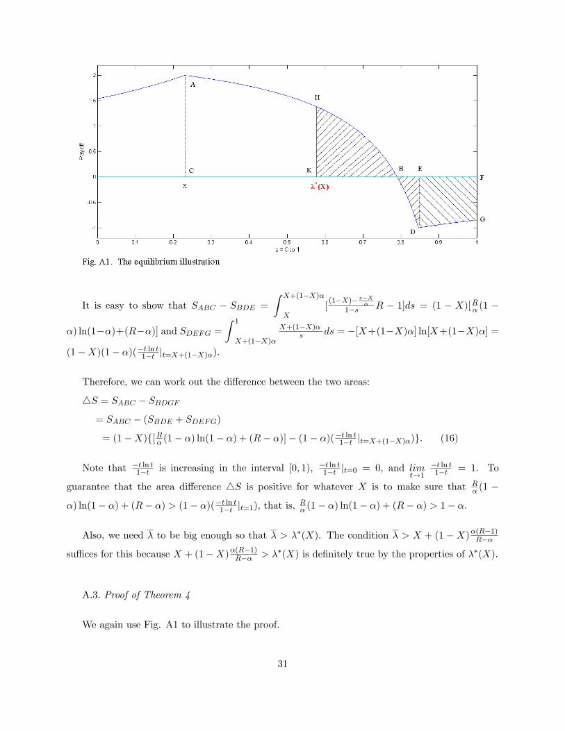
It is easy to show that SABC � SBDE =

Z X+(1�X)�

X[(1�X)� s�X

�1�s R � 1]ds = (1 � X)[R� (1 �

�) ln(1��)+(R��)] and SDEFG =Z 1

X+(1�X)�

X+(1�X)�s ds = �[X+(1�X)�] ln[X+(1�X)�] =

(1�X)(1� �)(�t ln t1�t jt=X+(1�X)�).

Therefore, we can work out the di¤erence between the two areas:

4S = SABC � SBDGF= SABC � (SBDE + SDEFG)

= (1�X)f[R� (1� �) ln(1� �) + (R� �)]� (1� �)(�t ln t1�t jt=X+(1�X)�)g. (16)

Note that �t ln t1�t is increasing in the interval [0; 1), �t ln t

1�t jt=0 = 0, and limt!1

�t ln t1�t = 1. To

guarantee that the area di¤erence 4S is positive for whatever X is to make sure that R� (1 �

�) ln(1� �) + (R� �) > (1� �)(�t ln t1�t jt=1), that is,R� (1� �) ln(1� �) + (R� �) > 1� �.

Also, we need � to be big enough so that � > ��(X). The condition � > X + (1 �X)�(R�1)R��

su¢ ces for this because X + (1�X)�(R�1)R�� > ��(X) is de�nitely true by the properties of ��(X).

A.3. Proof of Theorem 4

We again use Fig. A1 to illustrate the proof.

31

We express ��(X) as ��(X) = X + b(1 � X). Suppose X changes to X +4X. We want to

compare ��(X+4X) with ��(X). The idea of comparison is as follows. AfterX changes toX+4X,

the shape of the payo¤ curve of course changes because the parameter becomes X +4X instead

of X. We want to know under the new shape of curve whether the area di¤erence SBKH � SBDGFbecomes negative or positive if we still keep the threshold as ��(X). If 4S becomes positive, it

means that the above shaded area is bigger than the below one, that we need to remove part of

the above shaded area to make the two shaded areas equal, and consequently that ��(X +4X)

>��(X).

We check how the area di¤erence SBKH � SBDGF changes in two steps.

In the �rst step, we ask what the area di¤erence SBKH � SBDGF under the new curve is if we

keep b unchanged. That is, we want to �nd out the area di¤erence SBKH � SBDGF under the new

curve if the threshold is (X +4X) + b[1� (X +4X)].

It is easy to show SHBK � SBED = (1 � X)fR� [(� � �) + (1 � �) ln1��1�b ] � (� � b)g and

SEFGD = �[X + (1�X)�] ln[X + (1�X)�] = (1�X)(1� �)(�t ln t1�t jt=X+(1�X)�).

Because SHBK � SBED = SEFGD, we haveR� [(�� �) + (1� �) ln

1��1�b ]� (�� b) = (1� �)(

�t ln t1�t jt=X+(1�X)�). (17)

Therefore, @(SHBK�SBED)@X = �R� [(���)+(1��) ln

1��1�b ]+(��b) = �(1��)(

�t ln t1�t jt=X+(1�X)�).

Also, we can work out @(SEFGD)@X = �(1� �)(1 + ln t)jt=X+(1�X)�.

Overall, @(SBKH�SBDGF )@X = �(1� �)[�t ln t1�t � (1 + ln t)]jt=X+(1�X)�.

In the second step, we work out under the new curve how much the above shaded area SHBK

increases if the threshold reduces from (X +4X) + b[1� (X +4X)] to X + b(1�X). It is easy

to show that the area increases by (4X)(1� b)(��b1�b �R� � 1).

Aggregating the results in the above two steps, if the curve shape is changed with the new

parameter X +4X while the threshold is still ��(X), the area di¤erence SBKH �SBDGF becomes

(4X)f(1� b)(��b1�b �R� � 1)� (1� �)[

�t ln t1�t � (1 + ln t)]jt=X+(1�X)�g. (18)

32

Because �(1 � �)[�t ln t1�t � (1 + ln t)] is positive for any t 2 (0; 1), we conclude that b must be

decreasing with X. Hence the �rst term of Eq. (18) is increasing with X. Also, it is easy to

check that the second term (1 � �)[�t ln t1�t � (1 + ln t)]jt=X+(1�X)� is a decreasing function with

respect to X. Therefore, the whole term of Eq. (18) is increasing with X. To guarantee that Eq.

(18) is positive for any X 2 (0; 1), we need to have its value at X = 0 to be positive. That is,

(�� b) � R� � (1� b) > �� ln�� (1��)(1+ln�), where b solves (R� �1)(�� b)+

R� (1��) ln(

1��1�b ) =

�� ln�. Alternatively, the above inequality can be simpli�ed as R� ln(1��1�b ) < ln�.

In sum, ��(X) is an increasing function with respect to X if parameters satisfy R� ln(

1��1�b ) < ln�

(where b solves (R� � 1)(�� b) +R� (1� �) ln(

1��1�b ) = �� ln�).

A.4. Proof of Theorem 5

Again, we express ��(X) as ��(X) = X + b(1�X). We have @��(X)@X = (1� b) + (1�X) @b@X .

By Eq. (17), we have R� [(�� �) + (1� �) ln

1��1�b ]� (�� b) = (1� �)(

�t ln t1�t jt=X+(1�X)�).

Di¤erentiating on both sides of the above equation, we obtain R� (�

@b@X + 1��

1�b@b@X ) +

@b@X =

(1� �)2�(ln t)�1+t(1�t)2 jt=X+(1�X)�.

Thus, @b@X = (1� �)2

�(ln t)�1+t(1�t)2

�R�+1+R

�1��1�bjt=X+(1�X)�.

Therefore, @��(X)@X = (1� b) + (1�X)(1� �)2

�(ln t)�1+t(1�t)2

�R�+1+R

�1��1�bjt=X+(1�X)�.

After we work out the explicit expression of @��(X)@X , we can also explicitly express dW

II(X)dX , that

is,

dW II(X)dX = [(1 � R

� )X + 1��� ��(X)R] + [(X + (1 � X)� � ��(X)] � R� � [(1 � b) + (1 � X)(1 �

�)2�(ln t)�1+t(1�t)2

�R�+1+R

�1��1�bjt=X+(1�X)�]. (19)

Based on Eq. (19), we can directly evaluate dW II(X)dX at any X.

It is true that dWII(X)dX jX=0 > 0 and dW II(X)

dX jX=XC < 0 under general parameter values, which

means that there is an interior solution of X��.

A.5. Proof of Theorem 6

33

Because we know the expression of W II(X), the parameter conditions are the ones such that

W II(XC) < W II(X��). Such parameters do exist. The numerical example in the text is one case.

A.6. Proof of Theorem 7

Based on Eq. (19), we can directly evaluate dWII(X)dX jX=X� . Therefore, the parameter conditions

are ones such that dWII(X)dX jX=X� > 0.

A.7. Proof of Theorem 8

We need to prove only thatW I(X�; R) andW II(X��; R) are both increasing functions of R. For

W I(X) =

8>><>>:1�fZ X

0[(X � �) + (1�X)R]d�+

Z �

X[(1�X)� ��X

� ]Rd�g if X + (1�X)� � �

1�fZ X

0[(X � �) + (1�X)R]d�+

Z X+(1�X)�

X[(1�X)� ��X

� ]Rd�g if X + (1�X)� < �,

both (X � �) + (1�X)R and (1�X)� ��X� ]R are increasing in R. Therefore, when R increases,

W I(X�; R) increases even if we do not adjust X�. But, in fact, when R increases, X� changes as

well in maximizing W I(X). Therefore, W I(X�; R) certainly increases in R.

For W II(X) = 1�fZ X

0[(X � �) + (1 � X)R]d� +

Z ��(X)

X[(1 � X) � ��X

� ]Rd�g , we need to

prove that ��(X) is increasing in R �rst. In Fig. A1, as R increases, SEFGD is unchanged while

SBED decreases. So, if keeping ��(X) unchanged, SBKH � SBDGF > 0. Therefore, to restore

the equilibrium, ��(X) has to increase. After we prove that ��(X) is increasing in R, we use the

argument similar to that in the case of W I(X), and we can prove that W II(X��; R) is increasing

in R.

A.8. Proof of Theorem 9

In Fig. 7, the existence of a tiny proportion (�) of locked investors is equivalent to cutting a

�-width block at the right end of the below shaded area. So the below shaded area is reduced.

To make the two shaded areas equal, the above shaded area should be reduced as well. So the

threshold ��(X) has to increase. That is, for the same level of X, the survival window of the fund

is bigger if there is locked capital than that if there is not. Therefore, in the �rst-order condition

of Eq. (9), if we use the new increased threshold ��(X) to substitute for the original ��(X) while

34

keeping X the same, the �rst-order derivative becomes negative. That is, as the threshold ��(X)

increases, the optimal cash holdings become less.

35

References

Abreu, D., Brunnermeier, M.K., 2002. Synchronization risk and delayed arbitrage. Journal of

Financial Economics 66 (2�3), 341�600.

Abreu, D., Brunnermeier, M.K., 2003. Bubbles and crashes. Econometrica 71 (1), 173�204.

Allen, F., Gale, D., 2000. Financial contagion. Journal of Political Economy 108, 1�33.

Boyson, N.M., Stahel, C.W., Stulz, R.M., 2010. Hedge Fund Contagion and Liquidity Shocks.

Journal of Finance 65 (5), 1789�1816.

Brunnermeier, M.K., 2009. Deciphering the liquidity and credit crunch 2007-2008. Journal of

Economic Perspectives 23 (1), 77�100.

Brunnermeier, M.K., Pedersen, L.H., 2009. Market liquidity and funding liquidity. Review of

Financial Studies 22 (6), 2201�2199.

Calomiris, C., Kahn, C., 1991. The role of demandable debt in structuring optimal banking

arrangements. American Economic Review 81, 497�513.

Chen, Q., Goldstein, I., Jiang, W., 2010. Payo¤ complementarities and �nancial fragility:

evidence from mutual fund out�ows. Journal of Financial Economics 97, 239-262.

Corsetti, G., Dasgupta, A., Morris S., Shin, H.S., 2004. Does one soros make a di¤erence? A

theory of currency crises with large and small traders. Review of Economic Studies 71 (1), 87�113.

Dasgupta, A., 2004. Financial contagion through capital connections: a model of the origin

and spread of bank panics. Journal of the European Economic Association 2, 1049�1084.

Diamond, D., Dybvig, P., 1983. Bank runs, deposit insurance, and liquidity. Journal of Political

Economy 91, 401�419.

Diamond, D., Rajan, R., 2000. A theory of bank capital. Journal of Finance 55 (6), 2431�2465.

Diamond, D., Rajan, R., 2001. Liquidity risk, liquidity creation, and �nancial fragility: a theory

of banking. Journal of Political Economy 109, 287�327.

Goldstein, I., Pauzner, A., 2004. Contagion of self-ful�lling �nancial crises due to diversi�cation

of investment portfolios. Journal of Economic Theory 119, 151�183.

Goldstein, I., Pauzner, A., 2005. Demand deposit contracts and the probability of bank runs.

Journal of Finance 60, 1293�1328.

36

Gorton, G., 2008. The panic of 2007. Federal Reserve Bank of Kansas City symposium.

http://www.kc.frb.org/publicat/sympos/2008/Gorton.10.04.08.pdf.

Gorton, G., Winton, A., 2003. Financial intermediation. In: Constantinides, G., Harris, M.,

Stulz, R. (Eds.), The Handbook of the Economics of Finance. North Holland, Amsterdam, pp

431�552.

Gromb, D., Vayanos, D., 2002. Equilibrium and welfare in markets with �nancially constrained

arbitrageurs. Journal of Financial Economics 66, 361�407.

Johnson, W. T., 2006. Who monitors the mutual fund manager, new or old shareholders?

http://ssrn.com/abstract=687547.

Krishnamurthy, A., 2010. How debt markets have malfunctioned in the crisis. Journal of

Economic Perspectives, 24 (1), 3�28.

Mitchell, M., Pulvino, T., 2011. Arbitrage crashes and the speed of capital. Journal of Financial

Economics, forthcoming.

Morris, S., Shin, H.S., 1998. Unique equilibrium in a model of self-Ful�lling currency attacks.

American Economic Review 88, 587�597.

Morris, S., Shin, H.S., 2003. Global games: theory and application. In: Dewatripont, M.,

Hansen, L., Turnovsky, S. (Eds.), Advances in Economics and Econometrics. Cambridge University

Press, Cambridge, England, pp. 56�114.

Morris, S., Shin, H.S., 2004. Liquidity black holes. Review of Finance 8, 1�18.

Morris, S., Shin, H.S., 2008. Financial Regulation in a System Context. Paper prepared for the

Brookings Papers conference.

Morris, S., Shin, H.S., 2009. Illiquidity Component of Credit Risk. Unpublished working paper.

Princeton University, Princeton, NJ.

Plantin, G., 2009. Learning by holding and liquidity. Review of Economic Studies 76, 395�412.

Plantin, G., Sapra, H., Shin, H.S., 2008. Marking-to-market: panacea or pandora�s box? Journal

of Accounting Research 46, 461�466.

Rochet, J.-C., Vives, X., 2004. Coordination failures and the lender of last resort: was Bagehot

right after all? Journal of the European Economic Association 2, 1116�1147.

Shleifer, A., Vishny, R., 1997. The limits of arbitrage. Journal of Finance 52, 35�55.

37

Stein, J., 2005. Why are most funds open-end? Competition and the limits of arbitrage.

Quarterly Journal of Economics 120, 247�272.

38