Embed Size (px)
Citation preview

N 7 3 - 1 2 7 6 8 *
SPACE RESEARCH COORDINATION CENTER
THE FORMATION OF EXCITED ATOMS
DURING CHARGE EXCHANGE BETWEEN
HYDROGEN IONS AND ALKALI IONS
BYCASE FIL
COPYRONALD ALLEN NIEMAN
SRCC REPORT NO. 180
UNIVERSITY OF PITTSBURGH
PITTSBURGH, PENNSYLVANIA
1971
https://ntrs.nasa.gov/search.jsp?R=19730004036 2020-08-05T21:41:42+00:00Z

The Space Research Coordination Center, established in May. 1963. has die following functions: (1) it ad-ministers predoctoral and postdoctoral fellowships in space-related science and engineering programs; (2) it makesavailable, on app l ica t ion and after review, allocations to assist new faculty members in the Division of theN a t u r a l Sciences and the School of Engineering to initiate research programs or to permit established facultymembers to do preliminary; work on research Ideas of a novel character; (3) in the Division of the Natural Sciencesit makes an annual allocation of funds to the interdisciplinary Laboratory for Atmospheric and Space Sciences;(4) in the School of Engineering it makes a similar allocation of funds to the Department of Metallurgical andMaterials Engineering and to the program in Engineering Systems Management of the Department of IndustrialEngineering; and (5) in concert with the University's Knowledge Availability Systems Center, it seeks to assistin the orderly transfer of new space-generated knowledge in industrial application. The Center also issues pe-riodic reports of space-oriented research and a comprehensive annual report
The Center is supported by an Institutional Grant (NsG-416) from the National Aeronautics and Space Ad-ministration, s t r o n g l y supplemented by grants from the A.W. Mellon Educational and Charitable Trust, theMaurice Falk Medical Fund, the Richard King Mellon Foundation and the Sarah Mellon Scaife Foundation. Muchof the work descr ibed in SRCC reports is financed by other grants, made to i n d i v i d u a l faculty members.

THE FORMATION OF EXCITED AT&4S DURING CHARGE EXCHANGE
BETWEEN HYDROGEN IONS AND ALKALI ATOMS
By
Ronald Allem Nietnam
B.3., Carnegie Institute of Technology, 1963
Submitted t© the Graduate Faculty of
Arts and Sciences in partial fulfillment of
the requirements for the degree of
Doctor of Philosophy
University of Pittsburgh
1971

THE FORMATION OF EXCITED ATCMS DURING CHAR'S!
EXCHANGE BETWEEN HYDROGEN IONS AND ALKALI ATOMS
Ronald Allen Nieman, Ph.D.
University of Pittsburgh, 1972
Advisor: Thomas M. Donahue
The charge exchange cross sections for protons and various alkali
atoms have been calculated using the classical approximation of Gryzinski.
It is assumed that the hydrogen atoms resulting from charge exchange
exist in all possible excited states. Charge transfer collisions between
protons and potassium, as well as protons and sodium atoms have been
studied in this work. The energy range investigated is between k and
30 keV. The theoretical calculations of in&01 have been compared to
measurements of ff made in the course of this work as well as other
data. Also the calculated cross section for the creation of metastable
2S hydrogen has been compared to other experimental values. Good quanti-
tative agreement is found for 0 but only qualitative agreement for the
metastable cross section. Analysis of the Lyman alpha window in molecular
oxygen suggests that measured values of 0(23) may be in error. In
addition to ff-,Q, thick alkali target data are presented. - This allows the
determination of the electron loss cross section fffil. Finally, some work
has been done with H*.

FOREWORD
The author wishes to thank his advisor, Dr. T. M. Donahue, for
his patience, guidance and minimum of control. The aid of R. T.
Brackmann, W. R. Ott and W. E. Kauppila in the construction of the Geiger
tubes is appreciated. I also would like to applaud the constructive
genius of Morrie, Mac and the rest of the machine shop in putting
together the apparatus as it should be and not as I said it was to be.
To my cohorts and fellow drunks, thanks. I would like to thank Mrs.
Meriem Green, who took time out from running the Physics Department,
for typing this manuscript.
The author also wishes to acknowledge the works of another author,
a Mr. W. Shakespeare, whose words for a fitting motto for this work. As
Macbeth says in V.5. "Tis a tale,..".
This work was supported in part by Navy Grant NONR 62 -06.
TABLE OF CONTENTS
Page
FOREWORD . ii
LIST OF TABLES -1-33
FIGURE CAPTIONS 1 9
1.0. INTRODUCTION i
2.0. THEORY 7
2.1. Nomenclature 7
2.2. The Two Charge State System 8
2.3. Theoretical Description of n _.<?«, as a Function of
Energy 12
2.3.1. Introduction 12
2.3.2. The Adiabatic Criterion 12
2.3«3. The Born Approximation 13
2.3.4. Gryzinski Theory 17
2.4. Calculation of the Total Cross Section 18
2.4.1. Calculation of ffQ1 18
2.4.2. Calculation of 0,fr,0 22
2.5. Predicted Background Lyman Alpha Signal 25
2.6. Projected Lyman Alpha Signal 27
3.0. APPARATUS 29
3.1. Source and Ion Selector 29
3.2. The Charge Exchange Chamber 31
3.3. The Oven 31
3.4. The Detection Chamber 33
3.5. The Detectors 33
3.6. The Calibrators 36
iii
iv
Table of Contents ContinuedPage
3.7. Electronics 37
3.8. Gas Handling System hi
3.9. Vacuum Stands -t-2
3.10. The Oxygen Filter Vj
k.O. PROCEDURES FOR DATA TAKING 9
U.I. Data Taking U9
U.I.I. Introduction U9
U.I.2. Density Determinations 50
4.1.3. Neutral Fraction Determination 51
U.2. Typical Data Run 52
U.2.1. Charge Exchange Cross Sections . 52
U.2.2. Lyman Alpha Data 53
U.3. UV Detector Calibration 53
5.0. RESULTS 56
5.1. Charge Exchange Cross Sections 56
5.1.1. Measurements of ff and cr ; 57
5.1.2. H" Contributions and Orx and ffQy. 58
5.1.3. Inner Shell Contributions 58
5.I.U. Detailed Balancing Results 60
5.2. Deteimination of the Neutral Fraction Background ... 60
5.3. The Metastable Hydrogen 2S State 62
5.3.1. Sources of Metastable Atoms 62
5.3«2. Loss Mechanisms 63
5.3.3. Tentative Solution to the Case of the Missing
Metastables . 68
5.U. Excited Alkali Atoms 70

Table of Contents ContinuedPage
6.0. CONCLUSIONS ...... . . ................ 73
6.1. Overview . . . . . < , . < > ............... 73
6.2. Proton Bean . „ „ . .......... ,- ...... 7
6.3. H + Beam
6.k. H(2S) ..... ................... 75
6.5. General Remarks « , . . ................ 76
APPENDIX A; THREE COMPONENT BEAM CALCULATION .......... 79
A.I. Solutions of the Differential Equations ....... 79
A. 2. Alternate Derivation of the Basic Equation ...... 85
A. 3. Exact Evaluation of the Coefficients . . . ., ..... 87
A.I*-. Approximate Forms for the Coefficients ........ 90
A. 5. Hydrogen Molecular Ion as the Probe ......... 93
APPENDIX B: TRANSITION PROBABILITIES .............. 99
APPENDIX C: CALCULATION OF THE METASTABLE LIFETIME ....... 102
APPENDIX D; CALCULATION OF THE TWO WIRE FIELD .......... 115
APPENDIX E: A SHORT DISCUSSION OF NORMAL ERRORS OF MEASUREMENTS . 119
BIBLIOGRAPHY ...........................
TABLES ..............................
FIGURES ............................. 152
1.0. INTRODUCTION
Inelastic collisions between charged particles and neutral atoms
and molecules have been studied for many years. In the 1930's Tate,
Smith and Bleakney investigated interactions between electrons and
1-4atmospheric gases. Heavy ion interactions have been studied too.
Proton and atmospheric gas collisions have also been extensively
investigated. The theories that have tried to explain the results ob-
tained have involved approximations of one sort or another. The Born
approximation has been used for high energy interactions. Massey has
deduced a simple expression that involves physically reasonable quanti-
ties for a two body collision. This has provided insight into the
problems but has not been able to predict the cross sections.
For the simpler colliding partners there is now good agreement
between theory and experiment. However, even electron impacts with7
hydrogen atoms still yield surprises.' Of the many types of inelastic
encounters one of the simplest is charge exchange. The fast probe ion
captures an electron from the neutral target. Hasted tabulated many suchQ
cross sections. He was able to deduce a typical value for the effective
interaction distance. It is a few atomic diameters. Consequently, it
has become possible to predict the energy where the cross section is
largest but not its magnitude. Section 2.3.2 deals with this in more
detail.
An interaction that should be fairly easy to study is a proton
colliding with an alkali atom. Both reactants are hydrogen-like. Theory
and experiment compare favorably for the proton-hydrogen atom collision

9-11system. Furthermore, from the experimental point of view there is a
simplifying circ stance0 The removal of the target gas is expedited*
A large cold surface will condense the alkalis0 For example, at zero
degrees Celsius the vapor pressure of sodiua and potassiua are respec-
tively 2(-12)* Torr and l(-9) Torr. 2 With normal target gases the only
method of evacuation is to remove them with a high speed vacuw puap.
The cold trap method has been used before,, One recent usage was•• • ' ' • ' ' 1 3 ' . - . - . ' . • • .in the experiment of Putch and Daem, They puaped not only lithiwa with
such a surface but also water vapor. These two substances were neutral-
izers for protons0 .•:••"•
Recently interest has been aroused in proton-alkali reactions,.
Collisions leave the fast neutralized atoms in a highly excited state„
Plasma machines using magnetic mirrors were initially designed to build
the plasma by injecting fast H « At fifewt it was, thought that
dissociation of the fast ions by the residual gas would increase the
protqa «on«entration0 It was found charge transfer with these seme
residuals aatually removed the fast ions, A mechanism for dissociation
without collisions was sought* One such is the Lorentz force acting on
the ions as they move in the intense magnetic fields„ This effect ia
also mentioned in Section 5o5,2 on losses0• : 14 :
This general mechanism is called Lorentz ionizationo It would
be useful also for hydrogen atoms,, Highly excited atoms would be quite
15-17'efficiently ionized this way. In this injection method states belc
n•». 6 are not expected to contribute significantly since the radiative
*Throughout powers of ten are expressed in the above fashion; for example,2(-12) means 2 x 10"12, ; ' , ' : . ' ' " - . : ' :•
18lifetimes are too short. Those above n = 15 are generally ignored
because of their weak binding energies. They would be too easily ionized
19by fringe fields. Recent papers have been concerned with creating
those states in between.13'20'21
Besides this work on neutral injection, it has been discovered
these targets are useful for converting protons into H" for accelerators.
22 23Cesium seems to be the prefered alkali target for this purpose. ' J
ohDonnally discovered that with a cesivm target, metastable
hydrogen atoms were created from protons. He measured this cross section
from 160 eV to 3 keV. A listing of experimenters and their alkali work
will be given later. Other metastable sources recently used or discussed
25-27 9 28-30were proton-molecular hydrogen, proton-atomic hydrogen,
27 31 30proton-rare gas ' and atom-atom collisions. In addition I man alpha32
radiation had been seen during electron impact on Hp and proton-rare
26 33 3 4-gas and various ion-molecule cpllisions. '
Michal Gryzinski has published a series of papers on charged35-39
particle interaction. He uses classical mechanics and calculates
his results in the LAB frame instead of the traditional CM (center of
mass) frame. The approximate form for the charge exchange cross section
is very simple. There is good agreement with experimental values for
many cases. Modification of his simple theory has been carried out for a
togreat variety of collision partners. One example is presented herein.
For a proton probe and alkali target the binding energies are
well known. There seems to be no reason for excluding capture into all
excited hydrogen levels. Thus a sun of these cross sections is needed.
Throughout, the term "partial cross section" will refer to one of these.
The sum becomes a finite integral with a few simple assumptions. It is
possible to calculate the cross sections for electron capture into the
metastable 33, level as well as the total cross section.?
Calculations for the proton-alkali vapor interaction are presented
in Section 2. Cross sections for the two charge state are discussed. A
simple extension of Gryzinski's approximate foim for charge exchange is
the basis for computing various cross sections as a function of probe
energy. Total electron capture (o) values can be obtained this way.
The total cross section (TX) is the sum of many partial ones.
Particularly interesting is the cross section for the creation of hydro-
gen atoms in the first excited state. Some of these atoms will be in the
metastable 2S, state. This metastable cross section (MX) will be some.8
fraction of the cross section for capture into the first excited hydro-
gen state. Relative statistical weights place this fraction at 1/4. The
ratio of MX to TX can be calculated. The maximxm value would be 0.25 if
the states were populated according to their weights.
Whenever the above calculations are extended to include capture
of inner shell electrons, there is a noticeable change in the above
theoretical results. Usually for low energy protons, the valence electron
values dominate the cross sections. Beyond a few tens of kilovolts of
proton energy the inner shell contributions become Important.
The experimental and theoretical results of this work are
compared with those of other experimenters. Both TX and MX values are
collated. Until very recently no one group had measured both cross ;
sectipns for one alkali. Some anomalies appear in this compendium. They
will be discussed later.

Total exchange values have "been determined by groups working in
many countries. Cross sections have been measured by II'in, Oparin,
21 4lSolov'ev, and Federenko in Russia, Schmelzbach and coworkers in
42Switzerland, and Schlachter in this country. Principal investigators26.43 2k
of the metastable cross sections include Colli, Donnally and
44 45 46Sellin. ' Spiess, Valance and Pradel, working in France, found both
TX and MX for cesium,
TX values are measured in the present work for potassium and
sodium targets. The proton energy range is 4 to 30 keV. These TX values
21 4lcan be matched with those of II1-In and Schmelzbach. The equilibrium
neutral fractions (2.11) are also compared. Theoretical values for TX
42for cesium may be related to those obtained by Schlachter et al.
Metastable creation by charge exchange has also been noticed.
The modified Gryzinski metastable cross sections will be compared with
26 45those measured by Donnally and Sellin. Both have used cesium.
Cesium has been vigorously, if somewhat confusingly, investigated,
TX for rubidium has not been determined in this energy range. Sodium and
potassium are the convenient targets used here. Their cross sections
should differ by about a factor of two. Lithium should have the smallest
value of all the alkalis at any given energy. Table 1.1 lists the
various groups and the types of measurements they have taken.
The classical theory of Gryzinski is modified in Section II.
Comparisons are drawn between its predictions and observations with a
proton beam. In this work the protons collide with sodium and potassium
atoms. The ions are accelerated through 4 to 30 keV. The hydrogen
molecular ion probes the same two targets above 10 keVo Its -electron

capture cross section and its neutralized beam fraction for a thick
target are also measured. No calculations have been done for H_+ nor
have any other measurements been found for comparison,
A possible explanation for the greatly enhanced MX observations
is given. It involves the Doppler shift of UV radiation and the narrow-
ness of the transmission windows of oxygen. Some of the light will be
shifted outside the Lyman alpha window. This effect of the molecular
oxygen filter for the UV detector is somewhat fancifully described as
the "velocity dependent solid angle" of the Lyman alpha counter.
Resonant radiation has been seen in the exchange chamber. This glow
seems to be caused by excited alkali atoms.
The theory section - Section 2 - is followed by the description
of the apparatus. This includes the oxygen filter explanation in
Section 3.10. Data-taking procedures and sample data comprise Section k.
The results of the experiment and the calculations are given in Section 5.
The conclusions form the final segment of the body of this paper.
Various tangential matters appear in the appendices.

2.0. THEORY
2.1. Nomenclature
Consider a rearrangement collision in which a fast particle (B)
with initial Charge i^ encounters a target particle (A). After the
interaction the "beam particle has charge f_. This is written as
B1 + AJ - Bf + Ag + (f+g=i-j)e (2.1)
where the fast particle is written first. The following short-hand
notation could- also :be used; ••
AJ(Bi,Bf)AJ . (2.2)
oThe cross section for this reaction is written as ..0_ .
ij fgIn practice there is a stream of these fast ions which encounter
a localized aggregation of targets. This latter grouping is presented
in terms of a number density [n,(x)] which is a function of distance0
along the beam track. The subscript marks one of several targets than
can coexist in the region. The amber of particles with charge i_ varies
with the distance (x) along the track. If there are several reactions
converting charges from i_ to £, each one can involve different targets.
This can be written as
dNi(x) = ENf(x) O n(x)dx
* (2°3)

8
The source terms are collisions like (2.1) that convert net charge i_ to
final charge f. The loss terms remove £ by returning the-charge./state
to i. •-
For protons interacting with alkali atoms there are three such
charge states for the probe ion (1,0,-l). That case is treated in
Appendix A. If a negligible number of H" ions are formed, the equations
in the next section are adequate.
2.2. The Two Charge State
If only two charge states are possible, Equation (2.3) is greatly
simplified. It is more convenient, however, to discuss the fraction (F )
of the probe beam that has charge i_ instead of the number. This is
accomplished by dividing by the total number of bean particles. Further-
more, the total alkali density irrespective of charge is n . Let the
product n (x) dx be given by dw. The total electron loss cross section
(CLQ) and the total electron capture cross section (SQ-J) are given by
,_ s E v. E , .a_ [electron loss]10 J-0 J
-.n B E v Z a [electron capture]01 j=0 J g=0 OJ Ig
where v. = n./n,,, and En. » 1. Then the system of equations representedu J A J
by (2.3) becomes
DF° = -a F° + a F+ -01 10
(2o5)EF a -ff F + OF
10 01
where the symbol D is the differential operator d/dw. An additional
equation is
F++F° = 1. (2.6)
In the likely event of interactions "between discrete energy
levels of the reactants, the definitions of fractions and cross sections
in (2,5) should be extended. For example, electron capture by a proton
from a ground state sodiixu atom can be denoted by &* or o10 01 10 01
where the resulting hydrogen atom has its electron in level n. If the
atomic state is the metastable 2S, level, this cross section becomes3s 2s o9 . In the same way. the fraction of metastable atoms is F 00. In
10 01 \ 2Sorder to recover Equation (2.10 for this more detailed case, the following
new relationships are needed:
a = I VOh t,s ig oh
o t s
Since it is much more difficult to remove two electrons from an
alkali than one (the valence electron), Equation (2.5) should simplify.
The target will probably either neutral or, even less likely, singly
ionized. It is expected that (2.5) will reduce to
9 = 910 10 01
(2.8)9 => V 1 9 + 9 I + V I 9 + 9 I V » V01 o'oo 10 oo ii il 01 10 01 ii/ o i
where the cross section and the reactions with alkali target X are

10
p + X -* H + X+( ff ) [charge exchange]10 01
H + X - p + X + e ( a ) [stripping]00 10
H + X -* p + X+ + 2e( cr ) [ionization] (2.9)00 11
H + X+ •* p + X (01010) [charge exchange]
H + X+ -* p + X+ + e( o ) [stripping]
Since the X+ concentration is expected to be very small, the latter two
reactions should be negligible. The second of (2.8) will then just depend
on 9 and ff .00 10 00 11
Equation (2.5) can be solved by introducing (2.6). The resulting
first order differential equations can be readily integrated. The inte-
gration constants are evaluated by imposing the proper boundary conditions.
In this work there are collisions with the ambient background gas. These
produce a mixture of ions and neutrals impinging on the target region.
The boundary conditions are
F+(0) = 1 - 8
F°(0) . . . (
In this case the solutions to (2.5) become
,» = rL £ia(2.11)
1.0
HereCO
= aeo
CO
f drr s nie (2.12)Jeo
where t is the total length of the target region. The average density is
simply n. The usual experimental condition is thought to be a pure
11
proton beam incident on the target material. In that case 8 is zero and
Equation (2.11) simplifies „
There are two limiting forms for (2.11). One is the "linear"
approximation for w small,, The other is the high density "asymptotic"
value. These are
}*«! (2.13)w
and
The thick target values of (2.1*0 are independent of the initial neutral
concentration (6). The linear region depends on both 8 and the asymptote
(F°). Again the standard pure proton beam expressions may be recovered by
setting the initial fraction to zero. In this work the neutral fraction
(F°) is measured as a function of alkali density. The asymptotic value
(2.l4) can be used in conjunction with Equation (2.13) to determine the
cross sections in, this two state approximation. The slope, the intercept,
and the asymptotic values of (2.11) must all be measured as a function of
energy before a can be known,
It is important to note the convention followed here: calculated
cross sections will be denoted by Q but experimental ones by ff. Later,
attempts will be made to match theoretical cross sections (Qs) with the
measured values. For example, o will be compared with Q . In this
part of the theory section a was used^with the reactions. Explicit

12
values - cross sections calculated according to some theory - will "be
labeled Q. They so appear in the figures that follow the appendices.
2.3. Theoretical Descriptions of 9 as a Function of Energy10 01
2.3.1. Introduction
The interactions among an alkali core, a proton, and the valence
electron are too complex to be calculated exactly. In general three body
problems are beyond the capabilities of physics. Three useful approxima-
tions will be made for the proton to neutral cross section. The first is
rather qualitative. It is Massey's adiabatic criterion. The other two
are much more detailed. One is based on the Born approximation. The
other is the classical calculation done by Gryzinski.
2.3.2. The Adiabatic Criterion
For simplicity let the target atom be at rest. If the beam parti-
cle passes it very slowly, the electron cloud can adiabatically adjust to
the moving charge. If it passes very rapidly, the cloud cannot respond.
For the proper range of speeds the electron will be able to attach itself
to either charge center. The wave function will be a mixture of proton
and alkali core wave functions. Here the probability of capture by the
proton becomes large. Qualitatively then, the cross section for electron
capture by the proton will be small for both large and small velocities.
It will reach a maximum at the characteristic velocity vmax.
Whenever the period corresponding to the energy difference between
the two atoms at infinite separation (the energy defect) becomes compara-
ble to the transit time of the beam particle, the cross section is a
maximum. This time (t) is given by
T- ^— (2.15)max
13
where <a is a characteristic dimension of the system. It is a few
angstroms. Then the expression for vmax is
8Hasted has investigated this quantity for a variety of charge
exchange reactions. He has deduced a typical value for «i of 8A for
capture into the ground state. The energy defect for capture into the
second hydrogen level is about one electron volt (1.6 (-12) erg). Thus
%ax ~ 2.0 (7) cm sec . For a proton this corresponds to 200 eV, It
will be seen later that Gryzinski values peak near 1 key«.(See Table 2.1)
2.3»3« file Born Approximationk?
Early work on electron capture by Oppe nheimer and Brinkman and
kB U9Kramers was shown to have omitted an interaction term. Whenever this
50term was added, the resulting cross sections were too low, - The treat-
ment was extended to include capture into excited states.*7 Jackson and
Schiff used the Born approximation for their calculations. They were
able to relate their results to the OBK approximation. Bates andq
Dalgarno applied t&Ls correction to their OBK calculations. They pre-
sented explicit foims for capture into the first four hydrogenic levels.
The target atoms were also hydrogen- like. The captured electron cane
from the IS, 2S or 2P states. These calculations have been extended for
52capture into the first fifteen levels.
Consider the collision of a proton and a target atom. The ; -
electron is initially attached to charge Ze ja state ru, It is captured
into hydrogen state n . The cross section for capture from the state

vith principal quantua. auober n and azlmuthal quantum nuaber 1 into the• •;••.. ";•• ' .-.••• . ' -. :••'.• •" • -.- $ •'.. • • :•' •' " -.. •,
hydrogen state characterized by n and lf is
where
(2.17)
a » first Bohr radiuso • • ' . :-
C « constant
F • polynomial in x «
Jackson and Schiff deduced the following correction tern for a colli-
sion between normal hydrogen atone (IS) and protons;

15
itz
(2.18)
• pFor a proton probe the energy in keV is 2 .97 P »
For a metastable-like target the constants and functions vill be
rewritten as
(2,19)
For computational purposes it is somewhat better to change
variableso The transformations are
0 (2.20)-•G(a.)/»?-

Then Equation (2.1?) becomes
Yx
r(2.21)
A few constants and functions are
C(IS-IS) « 2 Z'
C(1S-2S) » 25Z5e
(2.22)
G(IS-IS) m z4
G(1S-2S) -' .B*(3
G(1S-2P) a z (.l-b2z)2
G(1S-2P) » Z5(l-b2z)
G(2S-n,p Jf) «s (l-2a2z)2G(lS-nftf)
In order to simulate electron capture from a ground state alkali
target, Q(2S-n £f) is computed for an effective charge Ze. This is
chosen such that the binding energy of the alkali becomes that of a
hydrogen-like 2S state. For potassium the effective charge is 1.130
times the proton chargei For sodium it is 1.229. As a first order

17
calculation then, assume the correction term [Equation (2.l8)j is the
same irrespective of initial and final states and charge Ze. The charge
exchange cross sections are shown in Figures 2-1 and 2-2. These Born
calculations indicate that capture into the first excited hydrogen level
dominates ground state transfer.CQ C^\
Butler, May and Johnston " have calculated cross sections for
charge exchange between protons and ground state hydrogen atoms. They
use the Born approximations, too. Their approximate cross sections for
hydrogen excitation are also very large. About one half of all excited
atoms will be present in the n = 2 level. Their cross sections peak near
17 keV.
2.3.1*. Gryzinski Theory
The third approximation is the classical mechanics calculation of
36-38Gryzinski. This allows cross sections to be calculated easily as a
function of beam energy and readily compared with experiment. The shapes
of these cross sections are in good agreement with this experiment.
The theory is extended slightly by allowing capture into all
excited hydrogen states. To keep the total cross section finite the
states are not weighted according to their total degeneracies. The
ground state has been excluded from this calculation. Whenever the cross
section is pathological - as it is for ground state capture?- it should
kobe calculated by detailed balancing. In that case the contribution
from the ground state is orders of magnitude less than that of the first
excited state. Accordingly it is neglected throughout. It is also
assumed that the substates are populated according to their statistical
weights. This assumption is unverified.
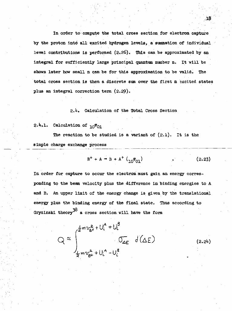
In order to compute the total cross section for electron capture
by the proton intd all excited hydrogen levels, a summation of individual
level contributions is performed (2«26). This can be approximated by an
integral for sufficiently large principal qjiantum number n. It will be
shown later how small n can be for this approximation to be valid. The
total cross section is then a discrete sum over the first sa sxcited states
plus an integral correction term (2.29)o
2,k, Calculation of the Total Cross Section
2<Xl. Calculation of jo Ol
The reaction to be studied is a variant of (2.l)» It is the
simple charge exchange process
B+ + A - B + A+ (1Qff01) V (2.23)
In order for capture to occur the electron must gain an energy corres-
ponding to the beam velocity plus the difference in binding energies to A
and B. An upper limit of the energy change is given by the translational
energy plus the binding energy of the final state. Thus according to
38Gryzinski theory a cross section will have the form
Q- OIe J(AE) (2.210
19
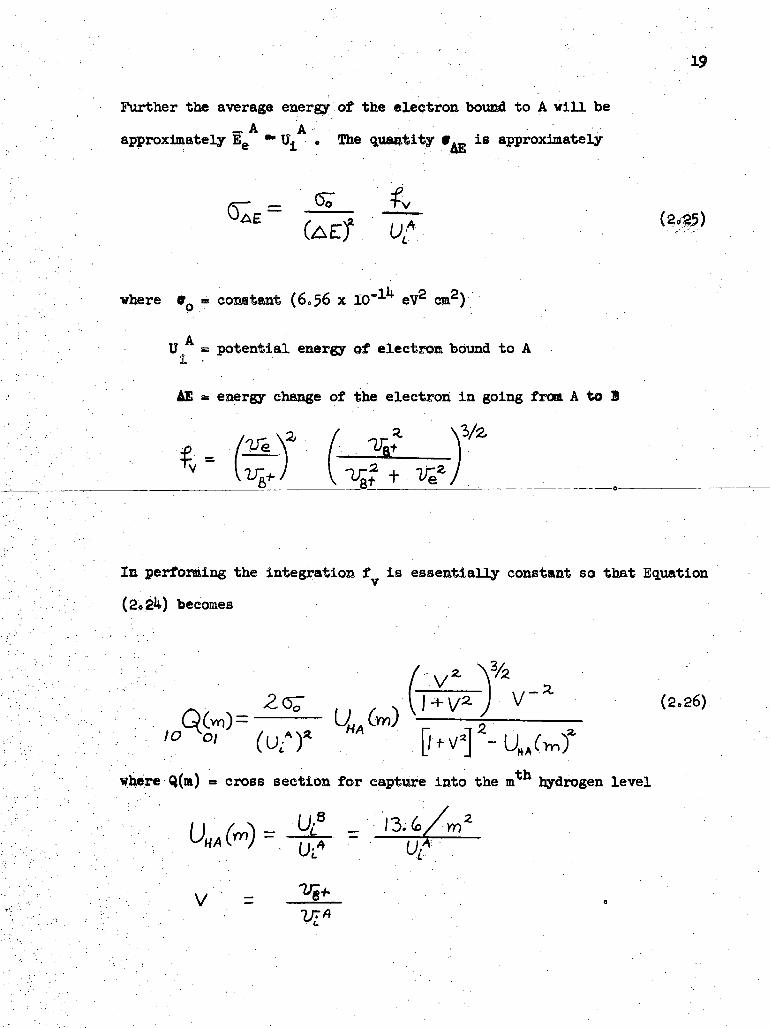
Further the average energy of the electron bound to A will be-A A
approximately ft *• IL . The quantity •._ is approximately; *"* i ' . nit*
(2.«)CAEir U*.
vhere e * constant (60 56 x'10"1^ eV2 cm2)0
AU s potential energy of electron bound to A
-
AE a energy change of the electron in going from A to 1
( J
In performing the integration f is essentially constant so that Equation
becomes
..v' (2<26)
where Q(m) = cross section for capture into the m hydrogen level

20
An estimate on the maxlmxm value for this cross section is Equation (lf.
of Reference 38;
Q + 2 4"(2c2T)
where a_ is the first Bohr radius
Z + is the beam particle charge
r • is the amplitude of oscillation of the target electrona . .
TJ
IL is the ionization potential of hydrogen (13.6 eV)«
These maxima are listed in Table 2olo
The smmatioa of these cross sections is performed in the above
mentioned manner<, The integration becomes
(2.28)
8/
where
It becomes then
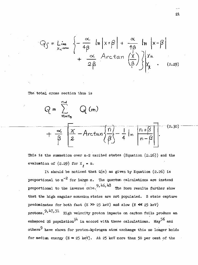
21
vy __
(2.29)
The total cross section thus is
od
"" p7T2
M fC. LO,r} i - >•1 1
4 '"
n f (3
*-p •
•C2T30-)-
This is the summation over n-2 excited states (Equation (2.26)) and the
evaluation of (2.29) for X «= n.
It should be noticed that Q(m) as given by Equation (2.26) isn
proportional to m for large m. The quantum calculations are instead
proportional to the inverse cube. s ! The Born results further show
that the high angular momeiotaa states are not populated. S state capture
predominates for both fast (E » 25 keV) and slow (E « 25 keV)
9 h-7 51protons. ' '" High velocity proton impacts on carbon foils produce an
enhanced 23 population'' in accord with these calculations. May and
9others-7 have shown for proton-hydrogen atom exchange this no longer holds
for medium energy (E « 25 keV). At 25 keV more than 50 per cent of the
22
captures will be into the I - 1 state. Only about one quarter are S
state captures'' *' as shown in Figure 2-3°
Figure 2-U shows the sum of a few discrete level cross sections
(Q(m)s) for electron capture from potassiwa. It should be noted that
about one half of the total contributions to the cross section come from
the first excited state. If the magnetic substates are statistically
populated, then approximately ten per ceat of the resulting excited level
cross section cones from the metastable 2S state. Also the rapid
convergence of the cross sections is easily seen,
Equation (2.30) has been compared with the discrete summation of
(2.26) for 200 levels. It was found that for most cases n = 11 is a
satisfactory lower limit for the integral. Figures 2-5 - 2-6 show the
theoretical cross sections for various alkali atoms. The predicted ratio
of metastables to total hydrogen atoms is also shown in Figure 2-7«
2.U.2. Calculation of 01»10
It was disclosed in the preceding subsection that the neutralized
probe particle will possess internal excitation. Thus the calculation of
the subsequent electron loss by this fast probe is more complicated than
that of Section 2. .1. The charge exchange reaction is
H» + A+ - p + A°(n)(0 J0) . (2.31)
The Gryzinski formalism - Equation (2.26) - becomes

23
01
(2.32)
where
MH
Although the alkali target above becomes the probe and the excited
hydrogen atom is its target, the projectile speed remains the proton
velocity. Equations (2.26) and (2*32) are identical for that well known
alkali, atomic hydrogen.
Equation (2.32) can be rewritten to show explicitly the
dependence on the hydrogenic principal quantum number (m) as
VI'
IV1-2
If 60?*J
(2.33)

24
This "becomes for a highly excited atom (large m)
01 u *
which is now independent of the hydrogen quantum number. Since
W ^C/ p/25 for keV energies, a ten per cent error is made by substi-
tuting the asymptotic foim (2.3k) for the exact Equation (2.33) for m = 7
at 5 keV and m » 3 at 25 keV.
Alkali binding energies do not depend as simply on the principal
quantum value as does hydrogen. However they do become hydrogenic for
large j-values as the quantua defect vanishes. Later the contributions
of alkali electrons more tightly bound than the valence electron will be
considered.
It can be seen that the cross sections (Equations (2.26) and
(2<> 33)) possess a pole where their denominators vanish. Naturally thekO
results there are unreliable. Garcia, Gerjuoy and Welker discuss this
and decide upon a useful change in the formalism. Whenever the limits of
(2.2U) allow this tangent-like discontinuity, Just apply detailed
balancing to calculate the offending cross section frcm the one corres-
ponding to the reverse reaction. For example, iQ Ol for the .creation of
ground state hydrogen is computed this way frcm QI^IQ* ' 'Their prescription
becomes
(2.35)
25
where 0* and u>- are the statistical weights of the initial and final<"' •••'" X
states of the original ;cross section. For a proton and the valence
electron of an alkali these weights are the same. For inner shell elec-
tron exchange they are not. Since half of the target atoms will have
their electrons wrongly oriented for capture, the reverse cross section
is divided by two. In Gryzinski theory the total cross section of a
state with energy E is the number of "equivalent" electrons with that
binding energy times the cross section of a single electron with energy
E,
2.5. Predicted Background Lyman Alpha Signal
One of the aims of this experiment is to determine the metastable
hydrogen (2S) population resulting from the charge exchange reactions.
This is done by applying an electric field to the neutrals and observing
Lyman alpha radiation. This mechanism is dealt with in Appendix C. It
is known from the preceding sections that all excited hydrogen levels
will be populated. Consequently there will be background radiation from
the natural decay of highly excited levels.
Since the hydrogen beam is optically thin (the density is about
1<y cm~ ), photon excitations can be neglected. Only the Einstein A
coefficients are needed. The population of the i sublevel obeys the
equation
—i- -N Ijk(l,j) +Z.N1k(j,i) (2.36)d-h 10 J 0dt

where the loss terms are transitions into lower lying levels and the
thsource terms are transitions down into this level from all of the J
levels possible. The k's are Just the Einstein A coefficients. They are
60 102tablulated in many places. '.' - .• To solve, (2;40) assyme N- (t) is given by
-H:t (2.37)
where
J= O for
and C(i,j) is the coefficient linking states i and j.
When this form is put into Equation (2o 0) and the various exponentials
are equated, the coefficients are seen to be
J
where 1 (0) is the initial population of the ith state.
This system of coupled differential equations represented by
(2.36) is solved for each t'iae.t-iby .substituting for the populations of
the higher levels. Such a repetitive procedure can be done easily on a
large computer such as the IM 7090. The number of levels that must be
considered becomes quite large. For the n state there are n sublevels.
For n states the number of equations is n(n+l)/2. For 10 states there
27
are two 55 x 55 matrices to be manipulated. For twelve levels they are
78 x 78. However for 20 states these matrices are 210 x 210 which far
exceeds the memory size of the 7090. Further, the running time of the
2calculation goes as n . In order to minimize the errors in neglecting
higher levels but to keep reasonable computing time, these coupled
equations were solved for a varying number of levels. 10 levels is a
good compromise.
The physics of this problem is in the initial population of these
levels. Gryzinski results from Section 2.U were used for this purpose.
Two different models were used: (l) the sublevels were populated
according to their statistical weights (2j+l); and (2) only the S sub-
levels were filled. The results of these calculations are displayed in
Figures 2-8 and 2-9.
2.6. Projected Lyman Alpha Signal
Lyman alpha radiation is "seen" by the UV detector which will be
described more completely in Section 3.5- The hydrogen beam passes
beneath it and emits background radiation. This comes from the cascade
of highly excited states mentioned previously. In order to detect
metastable 2S atoms a strong electric field is applied across the beam
path. Stark effect mixing of the metastable and resonance levels allows
depletion of the 2S state. The transition probability of the "metastable"
state is a function of the electric field intensity. Because of the high
velocity of the atoms, a very intense high electric field is needed to
quench the 2S state within some reasonable distance of the detector. The
28
STfield is too strong for the Bethe approximation - Equation (2.39) - to
be valid
1 = 2780 E2 (2.39)
\where f is the lifetime in seconds and E is the field strength measured
_T_in volts cm .
Equation (2. 3) fails for very weak as well as very strong
fields. The natural two photon radiative lifetime of one-seventh of a
second ' sets a upper limit. The lower limit to the lifetime is the
resonance value of 1.6 nsec. The calculations of Appendix C yield the
lifetime of the metastable state for the entire range of fields that will
be encountered normally. For more details see Appendix C (lifetime
calculation) and Appendix D (field configuration).
The UV signal received depends primarily upon the metastable
population, the geometry, and the efficiency of the detector and the
electronics. Supposedly the geometry is known. Detector response is
rather uncertain. It will be necessary to calibrate carefully and
thoughtfUlly.
Since the metastable state can be populated either by direct
interchange into the state (the ~) channel) or by cascase from higher
states (the ( _j channel), the beam energy enters into the population in
two ways. The cross sections are energy dependent. But, in addition,
the transit time from the oven to the detector depends on the square root
of the energy. The slower the beam, the more cascades occur. The dis-
tance between the oven and the UV detector is kO cm. Figure 2-10 shows
the expected ratio of metastable atoms to all atoms as a function of beam
energy. Figures 2-7 show the initial ratio for various targets.

3.0. APPARATUS
3.1. Source and Ion Selector
Figure 3-1 is a sketch of the apparatus. The ion source is a
commercial Duo-Plasmatron type which is capable of supplying several
millamperes of ion current. High purity hydrogen gas is bled into the
top of the source through a needle valve. No trapping of impurities is
done in the gas line since the source operates with the relatively high
pressure of 200 to 500 microns. Electrons are liberated from a number
80 mesh filament. To lower the work function of this 90$ rhodium - 10$
platinum filament the mesh is coated with a commercial oxide mixture.
Typical operating conditions for this filament are 6 volts AC and fifteen
to twenty amperes.
These electrons spiral in the field of a small electromagnet.
The poles of the magnet surround two sides of the source. It is clamped
to the three topmost plates. To minimize arcing problems between the
magnet and the source body the DC supply of the electromagnet is grounded
to the cathode. The field is variable.
The'.ions sit in a conical well until they are extracted through a
30 mil hole in the apex. Pumping holes are drilled into the sides of the
extraction cup located directly below the well. The current drawn by
this extraction process varies between 1.0 and 3.0 amperes. In order to
maximize the ion yield both this DC current and that of the magnet are
varied. In general low currents give the largest yield for low energy
ions whereas high energy ions require high arc and magnet currents. The
29
30
ions are accelerated through a high DC potential. This can be varied
from 0 through 30 kilovolts.
After leaving this middle portion of the source, the ions are
focussed by an electrostatic lens in the base of the source. The
potentials have been arranged so that the base plate, which is the third
element of the lens, is at ground potential. This requires that the
cathode be kept at the variable negative high voltage. As a result there
is no defocussing of the beam as it enters the grounded magnet chamber.
This brass magnet chamber sits between the poles of a large
electromagnet. Typically the field was ~200 Oe. The magnet runs on
highly regulated direct current. In order to exit this chamber the ion
beam must be bent through a 30 degree angle along a 15 inch radius. Any
one of the three major ions produced by the high pressure source can be
selected. In addition to creating protons and ionized molecular hydrogen,
the source also produces the HO ion in vast quantities. These three
ions are generated in approximately equal numbers.
To decrease the pumping load on the exchange chamber pump, the
magnet chamber has its own diffusion pump. It is an air-cooled two inch
pump manufactured by the Veeco Vacuum Company and rated at 80 liters per
second. The pump fluid is Dow Corning DC ?OU silicon fluid. This pump
can be valved off from the magnet chamber by a small tvo inch gate valve.
With this pump in operation the gas pressure under normal gas load is
-k2 x 10 Torr.
Normally the ions emerging from the magnet chamber are protons.
These ions are refocussed by an external einsel lens located between the
magnet chamber and the exchange chamber. The two outermost elements of

31
the lens are at ground potential. The middle element potential varies
from 0 to 6 kV DC.
3-2 The Charge Exchange Chamber
The charge exchange chamber is a cylinder 16 inches high and 10
inches in diameter. This stainless steel chamber has four equally spaced
two inch long arms welded halfway up the sides of the chamber. The beam
enters and leaves through two opposite arms. Below it hang a water baffle
and a ten inch water-cooled diffusion pump. This pump, which is made by
Consolidated Vacuum Corp. (CVC), is rated at M+00 liters per second
(unbaffled). It operates on 220 Volts 3 phase. Its pumping fluid is
also the low pressure DC 70 « Typical operating pressures under gas load
are 8 to 15 x 10 Torr with the magnet chamber pump operating. The
pressure doubles whenever the small pump is valved off. Normal condensi-
ble and alkali vapor trapping is done by a large cylindrical copper
shield. It surrounds five sides of the oven. It is connected to a
liquid nitrogen reservoir by a one inch diameter copper bar. Holes in the
shield allow passage of the ion beam. The background pressure for no gas
-7load but a cold nitrogen shield is 5 x 10 Torr. There is a viewing
port in the top of the chamber which allows observation of the space
between the shield and the front of the oven.
3.3. The Oven
The oven is made of Monel and has a rectangular base with a one
half inch diameter tube projecting symmetrically along the beam axis.
Flanges are attached to the ends of the tube. A plate is bolted to each
32
flange with 6-32 stainless steel screws, A metal 0-ring seals the plate-
flange connection. Apertures drilled into the plates collimate the beam.
The total length of the aims including the plates is 16 cm.
The target metal is slid along the arm into a well drilled into
the rectangular base. The oven is heated by two sets of independently
controlled heaters. One pair is mounted in the base and supplies most
of the heat for the oven. A secondary set is strapped to the arms. This
pair keeps the arms at a uniform temperature. At night they maintain
the arms at a higher temperature than the well. This insures that no
alkali is deposited in the arms between runs. The main heaters maintain
good thermal contact with the base. They fit snugly into the base.
Small screws press them against the sides of the holes.
Four chrom.el-alum.el thermocouples monitor the oven temperature.
One Junction in the base senses the well temperature. A second is screwed
to the top of the tube directly above the well. A third one is attached
to the "downstream" plate on the arm. The fourth is located on the arm
midway between the last two. The thermal E.M.F. is balanced against a
standard voltage in a bridge circuit that uses a small, relatively insen-
sitive galvanometer as the nulling device. Typical voltages are a few
millivolts.
The oven itself sits on three sharpened screws embedded in a
hanging platform. A bellows system and three external screws allow
spatial orientation of this platform. In addition it may be slightly
rotated about the beam axis by means of adjustment screws which push
against arms attached to the top plate of the bellows system. A hollow
stainless steel pipe passing through the top plate supports the platform.
33
It is now capped but could be used to supply gas to a standard gas target
cell should that be necessary.
3.U. The Detection Chamber
Between the exchange and detection chambers is a valve, a bellows
assembly, and a vacuum separator. The bellows allows the detector chamber
to be translated normal to the beam. The valve is also a CVC 2 inch gate
valve. The separator is a brass plate with a 3/8 inch diameter hole
drilled in the center. The detector chamber is identical to the exchange
chamber. It is pumped by a 6 inch CVC water-cooled oil diffusion pump.
The unbaffled pumping;:speed is l400 liters per second. It runs on single
phase 110 V alternating current. The fluid was initially DC 7C4 fluid
but later Convalex 10 was used. This pump has a CVC liquid nitrogen trap.
A single filling of nitrogen lasts for approximately k hours. A typical_7
background pressure is 3 x 10 Torr for the chamber valved off. Whenever_7
the connection is made with the exchange chamber, it rises to 5 x 10
Torr. Capacitor plates in the entrance arm are used to sweep the ions
from the neutral beam path.
3.5. The Detectors
Two major detectors hang in this chamber. They are the ion
detector and the Lyman alpha UV counter. The ion detector consists of a
thermocouple foil mounted inside a protecting Faraday cup. A grid, which
is 90$ transparent, is negatively biased to reject secondary electrons.
In addition the Faraday cup guard, the cup itself and the foil can all be
biased positively. These features are shown in Figure 3-2.

The thermocouple is a 1 mil thick Nichrome foil. It is sand-
wiched between 1% inch diameter rings. Three rings are copper; the
fourth ring in front is boron nitride. The heating effect of a particle
striking the foil is independent of its charge. Hence the foil can be
used to monitor neutral atoms. It is calibrated against the proton beam
by varying the beam current and noting the deflection on a nulling
galvanometer. This meter is part of a bridge circuit. Its standard
voltage is supplied by a mercury reference cell and a resistor string.
The voltage drops have been arranged in multiples of two for convenience.
The thermal E.M.F. is a few microvolts.
The junction is formed by contact between the foil and a small
copper wire soldered to the back of the foil. Current is drawn off
through a larger wire attached to the rings. The foil also integrates
beam fluctuations. It has a thermal time constant of h seconds.
A bellows system allows this detector to move in 3 dimensions.
Also the detector can be rotated through a slight angle (about 10°) in
the same manner, as the oven.
The UV detector, however, is fixed in space. It hangs on a bar
from the top plate of the chamber. The clamps that secure it to the bar
allow the detector to be repositioned somewhat. These clamps are not
accessible when the plate is bolted in place. Adjustments can only be
done whenever the chamber is open to the air.
63This detector is a modified Fite and Brackmann counter. It is
a cylindrical Geiger tube filled with a few crystals of iodine and argon
buffer gas. Constant iodine pressure is maintained by water cooling the
tube. A positive high voltage terminal collects electrons liberated
whenever a UV photon ionizes the iodine. The relevant reactions are
hv + I2".-* I2+ + e (photoionization) (3.1)
e + X - 2e + X+ (cascade) (3«2)
• e • * Ig I + I" (quenen) (3«3)
where X is the inert buffer gas. Here it is argon. The threshold for• • •
reaction (3d) is about 9<>7 eV (1270 A)» An oxygen cell ahead of the
detector limits the wavelengths that can enter the counter* Oxygen has
7 well known UV "windows"." One such absorption minimum occurs at the. . • . . . - . ' • • • • e
wavelength of Ionian alpha (1216 A). More will he said about this
molecular oxygen filter later. A lithiua fluoride crystal ^ seals the
counter. This single crystal is one inch in diameter and one-sixteenth
inch thick. Lithium fluoride has a short wavelength cutoff of 1080 A
which corresponds to 11.k eV."3
The filter is a chamber with a lithium fluoride crystal in front
and an 0-ring groove in back. A good vacuum seal obviates the need for
an additional piece of LiF. Screws fasten the cell to the face of the
detector. Oxygen flows through the chamber to prevent ozone build-up.
Since water vapor also has an extremely large cross section for layman67alpha, the gas is dried by passing it through a dry ice-acetone trap.
A light baffle is mounted in front of the oxygen filter. The
solid angle subtended by the detector (dO) is J**/383» Two wires hang
astride the beam path. Whenever high voltage is applied to these wires,
the quenching electric field is created. This is treated in detail in
Appendix D. The counter then observes part of the radiation. Figure
3-3 is a schematic representation of the detector and its electronics.
3.6. The Calibrators
Initially the UV counter was calibrated by means of a radioactive
source, it was swung into position directly below the detector. After
each data point was taken, the source was moved into place. The counting
rates for that day's run were then normalized using these calibrations.
Since there was so much uncertainty in the counter efficiency, an in situ
calibration was attempted.
In order to calibrate the UV detector its response to a known
32reaction is determined. Fite and Brackmann measured the cross section
for
e + Hp •* countable UV . (3. 0
oIt peaks at about 100 eV at 1.6 (-1?) cm and decreases monotonically.
A modified Pierce gun was built from commercially available parts. Its
prototype is described elsewhere. Normally the electron current to the
Faraday cup (the electron trap) was about 1% of that drawn from the
filament. It was possible to have currents on the order of 100 uA in a
1 cm spot for calibration. This gun is shown in Figure 3-^«
The gun filament was a strip of pure tungsten sheet 1 mil thick
cathode and 1/16 inch wide. It was maintained below the ground potential
of the second anode accelerating plate. The first plate was operated near
the filament. The electrons then fell through a total potential of a few
hundred volts. The beam is focussed by a three element lens. This con-
sists of the second plate, a short cylinder at several tens of volts, and
a flat sheet with a large (1/8 inch) aperture kept at ground potential.
The ion beams pass through a gap of several centimeters between this plate
and the Faraday cup guard. The guard is also grounded. The electron
36

37
trap is a 3 cm long cylinder closed at one end. To prevent electron
reflection from this cup, wire is coiled inside the trap and it is biased
slightly above ground, Typical operating voltages on these various gun
members are V ~ -150, Vp ~ -150, V, ~ 0 , V, ~ -60 and V^ ~ -60. Both
the last element of the lens (V/-) and the trap guard (V7) are grounded.
The trap itself (VQ) is ~2 volts. All of these parts are mounted on twoo
long ceramic rods which are not included in Figure 3-^»
These rods fit into two alxminum holders. These disks in turn
fit on vertical threaded rods. The holders are held in place by ordinary
nuts. The rods screw into a hanger which straddles the UV detector. The
gun can thus be oriented in space. Again these adjustments can be per-
formed only when the top plate is unbolted. Since the gun was to be used
only as a calibration device, no effort was expended in trying to make it
monoenergetic. The energy spread is consequently rather large, about 1
eV.
3.7. Electronics
The temperature of four locations in the oven is measured by
Chromel-Alumel thermocouples. Each one forms one arm of a standard bridge
circuit. The oven monitors pass through an octal vaeum feed-through.
An eight wire cable runs to a Leeds and Northrup thermocouple switch.
This special switch alternately selects the Junction to be nulled. No
reference junction is used. The various solder connections at room
temperature serve this purpose. Since the room temperature varies much
less than 1PF, it is much more constant than a naive, unprotected water-
ice system would be. The thermocouples are calibrated against several
standard points. Since some of these points are below room temperature
(about 70°F), the reference battery (a "D" cell) has a polarity reversal
switch.
Five standard temperatures are used. They are (l) the boiling
point of nitrogen, (2) carbon dioxide sublimation point, (3) the ice
point, (4) the water-steam point, and (5) the melting point of lead.
These values are listed in Table 3.1.
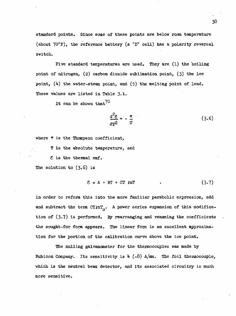
70It can be shown that1
dT2(3.6)
where T is the Thompson coefficient,
T is the absolute temperature, and
S is the thermal emf.
The solution to (3.6) is
£ » A + BT + CT InT . (3-7)
In order to reform this into the more familiar parabolic expression, add
and subtract the term CTfnT . A power series expansion of this modifica-
tion of (3.7) is performed. Ely rearranging and renaming the coefficients
the sought-for form appears. The linear form is an excellent approxima-
tion for the portion of the calibration curve above the ice point.
The nulling galvanometer for the thermocouples was made by
Rubicon Company. Its sensitivity is k (-8) A/mm. The foil thermocouple,
which is the neutral beam detector, and its associated circuitry is much
more sensitive.

39
The nulling device for the foil is a Leeds and Northrup model
galvanometer with a rated sensitivity of 0. 9 M-V/mm. To maintain
it at a uniform temperature it is kept in a plastic "box. Although the
metal case around the meter is grounded, additional shielding is provided
by wire screening around the "box. The time constant of the foil and its
circuitry is about k seconds.
The neutral detector leads pass through individual ceramic feed-
throughs. They terminate in female ERG connectors. The wires to the
bridge are RG-58/U coax. The current carrying ring wire is fed to a tee.
One branch is connected to the bridge. The other goes to ground through
the microammeter. The second lead is fed directly into the bridge.
The standard voltage for the bridge is supplied by a resistor
string across a 1.3U V mercury cell. There are 11 taps on this string.
The one per cent precision resistors are selected so that the reference
voltage varied by factors of two. Thus the minimum voltage is 2~ of
the maximun. The fine adjustment resistor is a ten-turn fifty ohm
precision potentiometer. A battery reversal switch and an off-on switch
complete the .controls on the bridge box.
The current meter that monitors the ring wire is an RCA model
WV-8 C Ultra Sensitive Microammeter. This is battery powered. The meter
range is about 2 (-10) to 1 (-3) amperes. Typical currents are a few
microamps. 'The input resistance is high (about 10" ohms). A shunt
capacitor of a few tenths of a microfarad is sufficient for integrating
a noisy signal.
The UV counter is powered by a Fluke 6000 VDC supply. Pulses pass
through a high voltage capacitor to a Hewlitt-Packard amplifier M/W
40
450AR. It has two fixed gains; it can "boost the input by either 20 or 40
dB. The amplified pulse is fed to a tee. Part of the signal is dis-
played on a Dumont oscillograph M/N 304-HR. The rest goes into a
Hewlitt-Packard 10,000 count sealer. The model H43-521CR sealer has
three fixed sampling times: 1/10, 1 and 10 seconds. In addition the
device has a provision for an external gate. By this a sampling time of
any desired length can "be selected. Data were taken with the 1 second
fixed time.
The Duo-Plasmatron ion source is powered "by a 30A transformer, a
DC power supply capable of delivering a few amperes to the small electro-
magnet, the arc supply and the voltage source for the einsel lens. The
large negative voltage on the filament, the arc and magnet supplies, and
the topmost plates of the source are furnished by a Sorensen M/N 1030-20
supply. It provides 30 kV at 15 mA. High voltage isolation transformers
allow line voltage to power the two floating supplies safely. The arc
supply gives a few hundred volts and up to 3 amps to the source to create
the two plasmas (H and Hg) in the extraction cup. The internal einsel
lens is powered by a Plastic Capacitors Model HV250-103M 25 kilovolt DC
supply. It is rated at 10 mA but the normal load is 1 - 2 mA.
Since the electron source for the Duo-Plasmatron consumes roughly
100 watts, water cooling is needed. A closed water system cools the fila-
ment electrodes, the 2 topmost plates of the source, and the middle
(ungrounded) element of the einsel lens. Distilled water is circulated
by a small pump from a refrigeration unit into demineralizer filters.
The chilled, filtered water flows through the hollow source plates.
The electron gun used a plethora of power supplies. The filament
is heated by a 25A 28V transformer. Two Kepco Model ABC-400 supplies

bias the cathode and the acceleration plate. Lens potentials are
furnished "by a 250 VDC Sorensen supply through voltage dividers. Small
voltages are provided by batteries.
3.8. Gas Handling System
The hydrogen for the source and calibration target comes from a
high purity tank through various valves and runs of copper tubing. Gas
goes from the tank through a standard regulator. It is connected to the
tubing through a threaded nut and shut-off valve. At a tee the flow
branches. It supplies the ion source directly. A valved branch line
feeds the calibration target. It has been explained previously how the
source cathodes are maintained at high voltage. The gas system is
grounded. A length of glass insulates the gas line at the source. It is
equipped with 0-ring sealed quick-couplers for easy removal. To prevent
ionization of the gas the needle valve is at source voltage. This makes
gas flow adjustments rather inconvenient while the source is operating.
The flow is set before high voltage is applied. The valve and glass
assembly is attached to the source through another coupler joint.
Meanwhile gas for the target flows through the valved tee branch
to a gas reservoir. This is another stainless steel vacuum chamber.
This chamber is 6 inches in diameter and 16 inches tall. It is similar
to the exchange and detector chambers in all respects. A 6 inch CVC
water-cooled oil diffusion pump evacuates the vessel. It is backed by a
Welch M/N 1936 fore pump. A water cooled baffle sits atop the pump
stack. Between the baffle and the chamber is a 6 inch gate valve. This

42
pumping station can clean the gas handling system as well as function as
a reservoir for the gas target.
3.9. Vacuum Stands
There are two stands supporting the vacuum chambers,, A long,
welded, steel table holds all but the reservoir chamber. This vacuum
chamber has its own stand. The reservoi-r bolts directly to its stand.
The rectangular top of this table is 16 x 24 inches. The top of the
stand is 48 inches above the floor. The pump stack hangs below the
chamber. The fore pump is below it. The base of the stand has adjustable
feet. The elevation can be changed by several inches. Physically it
stands beside the detector chamber at the foot of the long table. A
few inches of clearance are provided so that the detector chamber can be
moved,transverse to the ion beam.
The large table is also adjustable. It is 63" long and 24" wide.
Both the exchange and detector chambers roll on rails hung between the
side pieces of the table. The 10 inch diffusion pump limits the table
height. The fore pump backing this big diffusion pump is also located
outside the table. It sits beside the reservoir fore pump in the nook
formed by the two stands.
The large electro-magnet. is bolted directly to the table. The
ion source is clamped to the magnet chamber. However it hangs beyond the
back of the table. The entire table is angled into a corner of the room.
The source is thus relatively secure from falling bodies.
Sitting inside the side rails of the table are the fore pumps for
the magnet and detector chambers. The hydrogen tank is secured to the
front leg of the table. The liquid nitrogen reservoir for the detector
chamber juts beyond the table front.
3.10, The Oxygen Filter
At this point it is a good idea to examine ia detail the UV
counter and its molecular oxygen filter0 The detector that was used was
. . 63a modified Fite and Brackmann (FB) counter. The buffer gas used was
one half atmosphere of argon instead of the helium of Reference 63. This
design modification of Ott ' produces a good plateau, i.e., the
counter sensitivity is essentially independent of applied voltage.
The properties of such a counter were investigated by Fite and
others. ^ The angular and radial sensitivity of the original counter
design and its temperature dependence have been reported. The lithium
71fluoride windows have been discussed by Schneider (index of refraction)
and Ott ° (transmission of polarized Ionian alpha radiation).
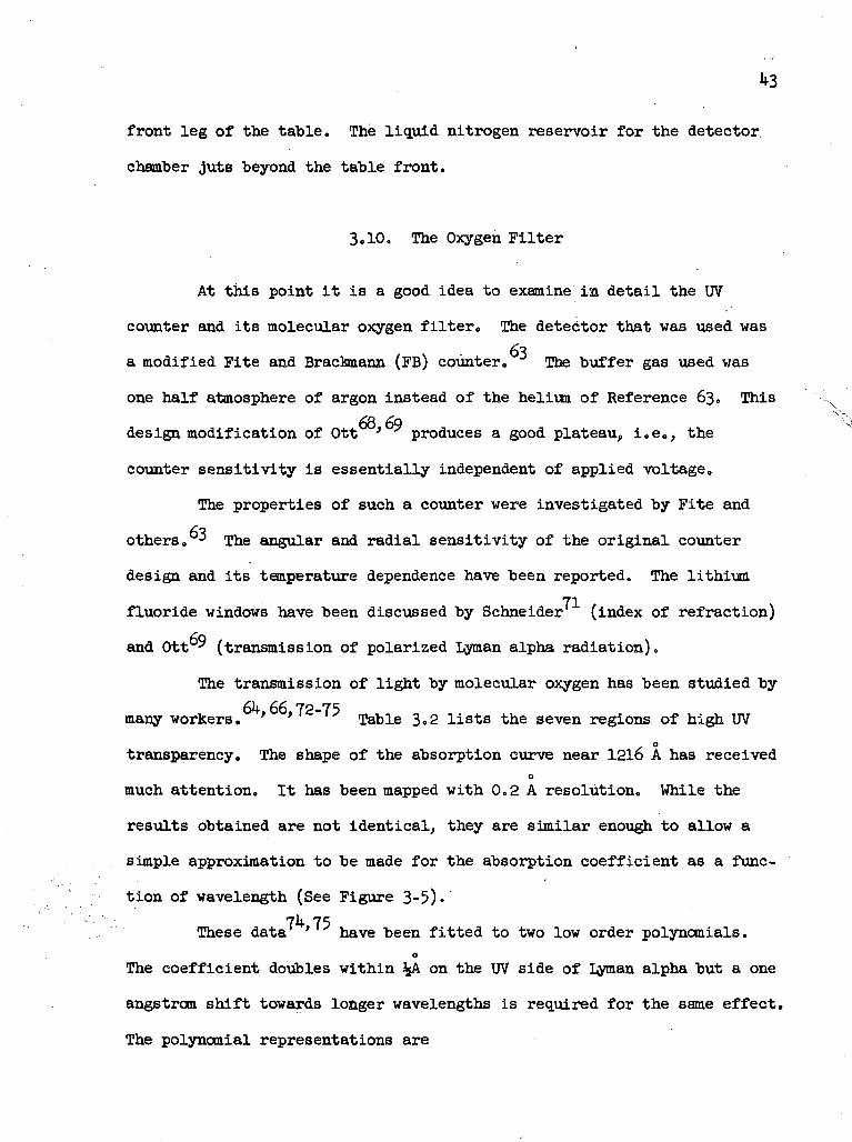
The transmission of light by molecular oxygen has been studied by
many workers. ' ' Table 3.2 lists the seven regions of high UVo
transparency. The shape of the absorption curve near 1216 A has receivedo
much attention. It has been mapped with 0,2 A resolution. While the
results obtained are not identical, they are similar enough to allow a
simple approximation to be made for the absorption coefficient as a func-
tion of wavelength (See Figure 3-5).
74 75These data ' have been fitted to two low order polynomials.o
The coefficient doubles within %A on the UV side of I rnan alpha but a one
angstrom shift towards longer wavelengths is required for the same effect.
The polynomial representations are
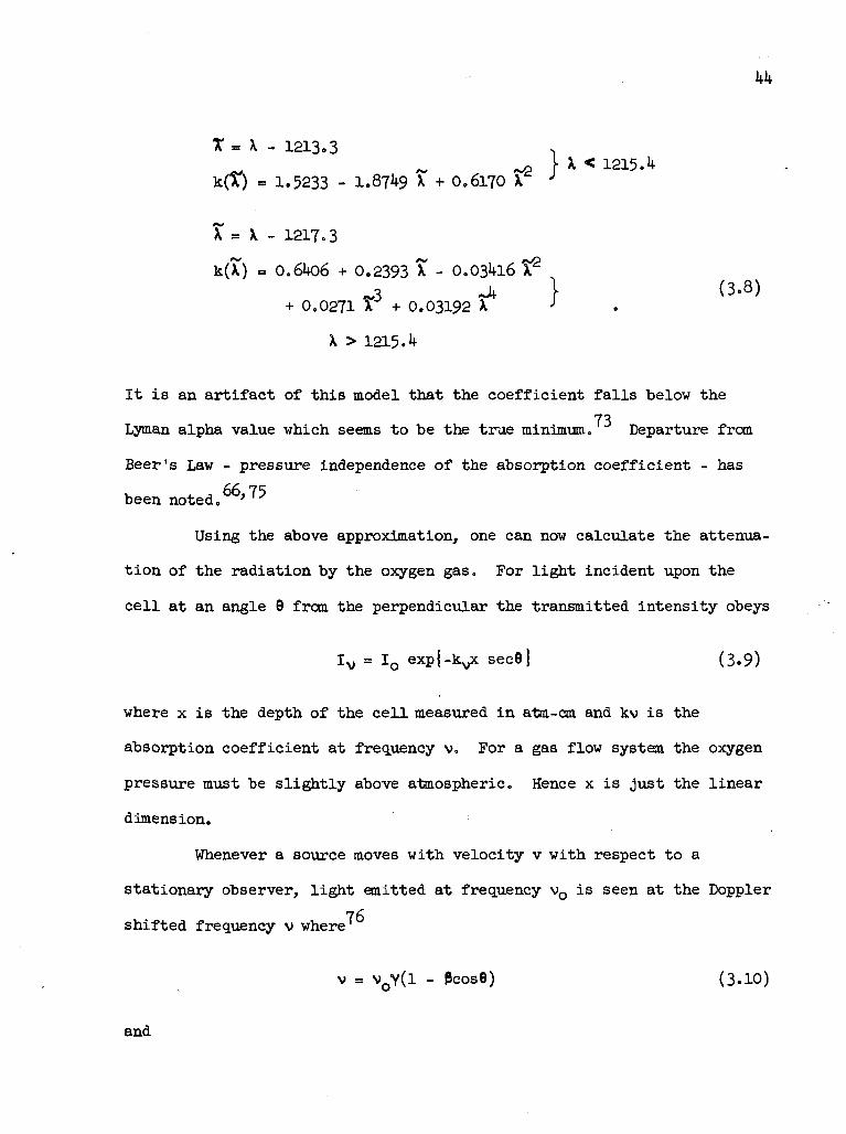
* = X - 1213.3 -,„ ~ ~? r x < 1215. !
k(X) = 1.5233 - 1.87 9 X + 0.6170 X J
\ = x - 1217.3= o.6lK>6 + 0.2393 t - 0.03^16
~3 *A+ 0.0271 x + 0.03192 xX >
It is an artifact of this model that the coefficient falls below the
73Lyman alpha value which seems to be the true minimum. Departure from
Beer's Law - pressure independence of the absorption coefficient - has
been noted.66'75
Using the above approximation, one can now calculate the attenua-
tion of the radiation by the oxygen gas. For light incident upon the
cell at an angle 9 from the perpendicular the transmitted intensity obeys
Iv = I0 expl-k^ sec9} (3.9)
where x is the depth of the cell measured in atm-cm and kv is the
absorption coefficient at frequency v. For a gas flow system the oxygen
pressure must be slightly above atmospheric. Hence x is just the linear
dimension.
Whenever a source moves with velocity v with respect to a
stationary observer, light emitted at frequency vo is seen at the Doppler
76shifted frequency v where
v = vQY(l - PcosO) (3.10)
and

v/c
In this work v/c « 1/150 so that Equation (3olO) can be approximated by
v = vo(l-3cose) + %VQ32 (3.11)
where the first term is the classical Doppler shift and the other is
called the relativistic shift. This one is always towards the red
(longer wavelengths) whereas the classical shift varies from, red to blue.
Thus the net shift is redward. Since the absorption coefficient curve is
also asymmetrical, the strange curves of Figures 3-5 and 3-6 result from
Equation (3«9)« The parameter for the family of curves is the proton
energy in keV.
Since absorption by the oxygen can limit the acceptance angle of
the counter more severely than a geometrical aperture, it seems natural to
extend the notion of a solid angle and call this a "velocity dependent
solid angle".o
The relativistic shift for a 30 keV beam is only about 25 mA. For
beta values one order of magnitude larger than those encountered hereo
this shift moves the apparent source of "line center" (1215.67 A) radia-
tion appreciably. The region that emits this radiation travels farther
upstream -towards the oven as the energy increases . The apparent light
source can be outside the field of view. In this case a small slit would
loose too much I man alpha radiation. For the energies typically
encountered in this experiment a geometrical angle of 5° will lose 20 per
cent of the light. Figure 3-5 shows the relative transmission of the

oxygen as a function of the complement of 6, viz., 6. Figure 3-6 is the
integrated intensity of the light as a function of the geometrical half-
angle (60) and the energy.
This velocity dependence of the solid angle will wreak havoc with
33 77calibrations. Some workers have worried about the Doppler shift. '
The extent of their concern about the standard calibration procedure is32
not known. This method consists in colliding electrons with thermal
molecular hydrogen. Countable UV is created. When metastable atoms are
quenched, their energy is several thousand electron volts. Consequently
the solid angles may differ considerably.
For purposes of illustration suppose that the counting rates are
proportional to the cross section and the solid angle. This is a low
density target. One then has
R dfl
IT
where the subscript "c" stands for calibration and "x" for the experiment,
dfi varies with beam energy. Above 10 keV it is relatively constant. AtJ\.
lower accelerating voltages a slight energy variation changes beta
rapidly and with it, the solid angle. Since dC^ is velocity dependent,
the measured cross section (ev} will be too small unless this effect isA
noted. If the rates were equal and the velocity dependent solid angle
were twice the "thermal" one, ffx would actually be twice 9Q. A naive
calculation would have called them equal instead. The calibration
correctly gauges the angular and radial counter sensitivities but not the
geometry.

Unless special precautions are taken, Lyman alpha can scatter
into the UV detector. This light reflects from metal surfaces. It will
have undergone: audifferent Doppler shift than the directly viewed radia-
tion. The virtual emitting region can be much bigger* than the real.
Light that travels directly downward under the FB detector, strikes a
horizontal surface, and reflects upward into the counter will add a
constant background to the directly viewed radiation. This reflect light
will be shifted less than the equivalent direct light. For faster meta-
stables the frequency of the scattered light moves towards higher attenua-
tion values. .'AM so its signal decreases. Such an effect is noticeable
in the data of Sellin and Granoff. Their measurements show an abrupt
Jump near 10 keV that can be explained by this scatter-shift hypothesis.
There is a large caveat to be connected to the above calculations:
Nature is not simple. At least four effects should be included in
quantifying the response of the filter to Lyman alpha. First, the beam
is a three-dimensional entity. It is more or less a cylinder. This
finite extent of the source should be included in a more complete calcu-
lation. Secondly, impurities such as water vapor or ozone will wash out
the absorption minimum. A third point is that the curves were derived
using values of the absorption coefficient for low pressure. Preston
75and Watanabe" have observed a linear pressure effect on this coefficient
for line center Lyman alpha radiation. The attendant change at nearby
wavelengths is unknown. Preston suggested that the minimum lies near a
weak oxygen band. At atmospheric pressure the absorption curve could be
even more distorted than it is for low pressure.
Finally, the calculation was performed under the assxmption that
the photons vanish from the beam. As a result of multiple scatterings in

the oxygen, some will actually emerge from the cell and enter the counter.
This is a radiative transfer problem. The photon flux consequently is
too low. The impurity effect will decrease this flux but increase the
effective acceptance angle of the detector. The baric changes will
probably decrease both the angle and the transmission.
78Although "gold black" deposits reduce the reflection of layman
79alphas from metallic surfaces, visible as well as ultraviolet
radiation is emitted whenever ions strike such surfaces. The light
intensity is strongly dependent.on both the beam current and its angle
of impact with the surface. Such countable UV has been observed in this
experiment too. When protons hit the rod holding the radioactive source
calibrator (Section 3«6)> the counting rate was markedly increased.

4.0. PROCEDURES FOR DATA TAKING
4.1. Data Taking
4.1.1. Introduct ion
The "basic data taken are the neutral beam, fraction (F ) and
target density (n(x)). These are measured as a function of probe energy.
The triad of fraction, density and energy are adjusted in four simple
vays. The simplest is to fix the beam energy and vary the alkali density
over a narrow range. This is the low density (LD) method. The neutral
fraction is approximately a linear function of target density (see
Equation (2.13)). A related method is to look at two or three different
energies and slightly vary the density. This is basically performing
several LD runs at once. Of course the number of measurements that can
be taken for each energy is lessened. This cross section normalization
method is useful in normalizing sets of results. It is used mainly as an
overview of charge exchange reactions, especially for the HQ+ beam inter-
acting with the alkalis.
The third main run type is the complete curve (CC) run. Again
the beam energy is fixed. This time the oven temperature is increased to
such a high value that the high density asymptote (C ) is reached. There
the neutrals obey (2.14). The fourth type is done very infrequently.
The oven stays very hot. This creates a thick target. This run type
verifies the asymptotes already found by CC runs or measures them for a
variety of energies.
50
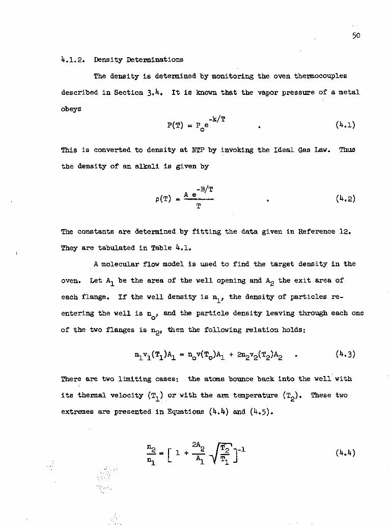
1*-. 1.2. Density Deteiminations
The density is determined by monitoring the oven thermocouples
described in Section 3.4. It is known that the vapor pressure of a metal
obeys-k/T
P(T) m PQe . (4.1)
This is converted to density at NTP by invoking the Ideal Gas Law. Thus
the density of an alkali is given by
-B/Tp(T) = £-2 - . (4.2)
T
The constants are determined by fitting the data given in Reference 12.
They are tabulated in Table 4.1.
A molecular flow model is used to find the target density in the
oven. Let AI be the area of the well opening and Ag the exit area of
each flange. If the well density is n,, the density of particles re-
entering the well is n , and the particle density leaving through each one
of the two flanges is n2, then the following relation holds:
There are two limiting cases; the atoms bounce back into the well with
its thermal velocity (T,) or with the arm temperature (T2). These two
extremes are presented in Equations (4.4) and (4.5).

J £ _ r , , 2^1-1ri+ rs-i-i fiL ^J.-VT.
Typical operating temperatures are T., ~ 500°K and Tp ~ 450°K.
Equation (4.4) can be approximated as
T - T1 2
For the above temperatures the discrepancy in densities is less than
3 per cent.
4.1.3. Neutral Fraction Determination
For one data point the total beam falls upon the foil thermo-
couple (D. . ). The bridge circuit is used to null the generated E.M.F.
The reading of the fine adjustment pot is recorded as I>tot. The coarse
control is always adjusted so that the null position is at least half way
(500) on the fine pot. Since experimenters normally have five fingers on
each hand, there is a bias towards recording readings in multiples of
five. This "half way" precaution keeps this bias error small.
High voltage is applied to the capacitor plates at the entrance
to the detector chamber. The ions are swept from their original beam
track. The lessened heating effect is noted (Dn). Small contact poten*-,.
tiale are determined by turning off the beam and recording the galvanome-
ter deflection (D _„). Then the sought-for neutral fraction is just
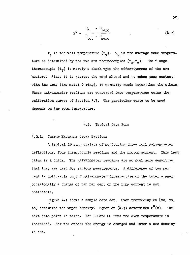
52
DM - Dn zero
D. - Dtot zero
Tn is the well temperature (t ). T0 is tlie average tube tempera-.L ** £»
ture as determined by the two aim thermocouples (t_,ta). The flange
thermocouple (tf) is merely a check upon the effectiveness of the arm
heaters. Since it is nearest the cold shield and it makes poor contact
with the arms (the metal 0-ring), it normally reads lower,than the others.
These galvanometer readings are converted into temperatures using the
calibration curves of Section 3«T- The particular curve to be used
depends on the room temperature.
4.2. Typical Data Runs
4.2.1. Charge Exchange Cross Sections
A typical LD run consists of monitoring three foil galvanometer
deflections, four thermocouple readings and the proton current. This last
datum is a check. The galvanometer readings are so much more sensitive
that they are used for serious measurements. A difference of two per
cent is noticeable on the galvanometer irrespective of the total signal;
occasionally a change of ten per cent on the ring current is not
noticeable.
Figure 4-1 shows a sample data set. Oven thermocouples [tw, tan,
ta] determine the vapor density. Equation (4.7) determines F (TT). The
next data point is taken. For LD and CC runs the oven temperature is
increased. For the others the energy is changed and later a new density
is set.

53
k.2.2. Lyman Alpha Data
Whenever I man alpha radiation is to be monitored, the above
procedures change. Normally an LD run is made. At the same time the
photon counter is activated. While the total beam - both protons and
neutrals - enters the detector chamber, this counting rate is recorded
(NF). Then the dipole field is applied. The metastables are quenched.
This rate is recorded (F). Whenever the foil galvanometer zero is being
determined, the background signal (BG) is noted. .'The number of meta-
stables is then proportional to F-NF. The cascade signal is NF - BG.
The proportionality constant (S) is the same for both. It was to have
been determined by the electron gun calibration. This tale appears
later. Typical counter data are presented in Figure lv-2. The above
naive picture must be modified somewhat. Just as the quench field
mixes the levels of the first excited state, it also mixes the other
levels. Further it will be seen in Appendix C that some of the
"resonant" levels live longer.
U.3. UV Detector Calibration
The counting rate of the sealer depends upon the number of
photons that can be transmitted by the optical train. The propor-
tionality constant (xi) between the photons emitted and the counting rate
is given by
s - *n § A>EcV (M)

where dO is the solid angle subtended by the beam
dS is the area of the detector
R is the distance from the beam to the detector
T is the transmission of the LiF crystal
T is the transmission of the oxygen
EC is the counter efficiency
Ee is the efficiency of the electronics,
2The quantity dfldS/R is called the throughput of the optics. It is
readily measurable. The transmission of the crystals is approximately
69one half. For oxygen at NTP the extinction length is extrapolated to
1/0.65 cm. Thus the transmission (T ) is 0,278. However the counter
response is strongly temperature dependent. The photoionization effi-
ciency (reaction (3«l)) is approximately O.lj-2 but the iodine density
follows Equation (*K2).
In addition to this counter response, the iodine reactions limit
the number of photons that can trigger the detector. This dead time
69effect has been calculated. The notation used there is slightly
different from that used here. The observed counting rate (RQ) must be
corrected for the counts that are lost while the Geiger tube is recovering
Tfrom the previous pulse. Let the maximua rate as determined by the dead
time be designated as R . The actual rate (RQ) becomesx a
Typical pulses after hQ dB amplification are 1 volt high. The peak occurs
kO (jisec after onset. The recovery time is about 250 p,sec. The next

55
triggering pulse occurs approximately 350 usec after the onset. This
differs somewhat from other counters. "
AC fields are present in this interaction region. They come
primarily from the ripple on DC power supplies. In order to lessen their
effect on the scalar discriminator, a 120 Hz trap was installed between
the amplifier and the sealer. It is. estimated that the electronics pass
one half of the signal pulses. To simplify calculations the calibration
runs should ideally produce the same rates as data runs,
In light of the filter discussion in Section 3.10 and the
63published angular response of the UV counter, H is actually dependent
on temperature and emitter position.
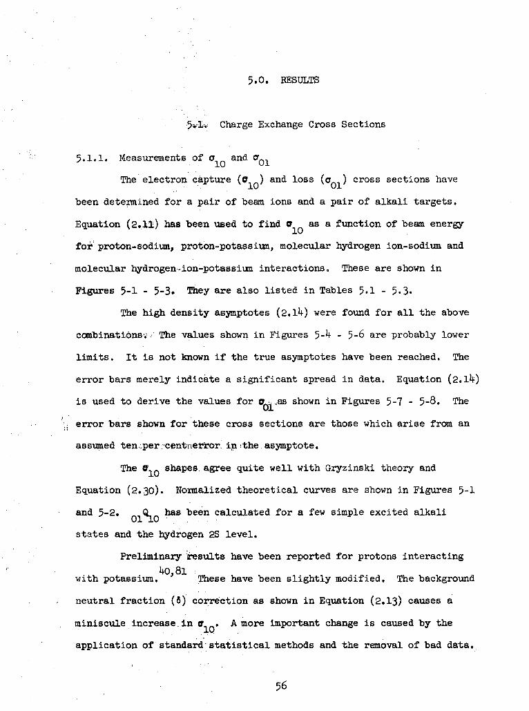
5.0. RESULTS
.:-5»lv Charge Exchange Cross Sections
5.1.1. Measurements of a and OQ
The electron capture (3,n) and loss (om) cross sections have
been determined for a pair of beam ions and a pair of alkali targets.
Equation (2.11) has been used to find 9 as a function of beam energy
for proton-sodium, proton-potassium, molecular hydrogen ion-sodium and
molecular hydrogen-ion-potassium interactions. These are shown in
Figures 5-1 - 5-3. They are also listed in Tables 5.1 - 5.3.
The high density asymptotes (2.1*0 were found for all the above
combinations* .<'• The values shown in Figures 5-^ - 5-6 are probably lower
limits. It is not known if the true asymptotes have been reached. The
error bars merely indicate a significant spread in data. Equation (2.
is used to derive the values for o- ;as shown in Figures 5-7 - 5-8. The
•,;. error bars shown for these cross sections are those which arise from an
assumed ten:per::-centnetror, in <• the asymptote.
The 9-o shapes, agree quite well with Gryzinski theory and
Equation (2.30). Normalized theoretical curves are shown in Figures 5-1
and 5-2. Q has been calculated for a few simple excited alkali
states and the hydrogen 2S level.
Preliminary results have been reported for protons interactingU0,8l
with potassium. These have been slightly modified. The background
neutral fraction (6) correction as shown in Equation (2.13) causes a
miniscule increase in a . A more important change is caused by the
application of standard statistical methods and the removal of bad data.
56

57
5.1.2. H" Contributions and cr— and o-r-
An upper limit on the amount of H" ion produced is about three
per cent below 10 keV. This comes from deducing the negative ion current
that would diminish the ring current enough to affect the inferred posi-
tive flux. The difference between total beam and neutral beam heating1
can be ascribed almost entirely to the positive current monitored. Above
10 keV no H" seems to be formed. A reasonable limit is one per cent.
If there were appreciable negative ions in the beam, the complete
curve data (CC) of U.I.I would deviate from the simple exponential expres-
sion of (2.1l). The H" concentration should be small. Its most probable
osource is charge transfer with H . Proton interactions with cesium
42create no more than 3 Pgr cent H" above k keV. The simple form of
Equation (Ak6) should be usable here. The difference between the data
and the simple exponential was examined for <7y and O~— as set forth in
Appendix A.
A series of test cases was run. The high density asymptote was
found very accurately. The determinations of a and 0 depended upon the
relative sizes of A and B. This is proper. Actual data were then put
through this procedure. The results were quite definite. Two exponen-
tials always fit the data worse than just one as given by (2.11). Since
some of the parameters of the extended fit interact, their number was
reduced from 5 down to 3 eventually. Successive iterations were also
used. At1 the very best the errors associated with this extended fit
nearly equalled thosecipf the simple exponential. By this time, however,
the parameters had changed drastically from the initial guesses, a and P
showed an infuriating tendency to approach one another.

58
There are three disturbing possible explanations for this
failure. The obvious one is that there is too much scatter in the data
from random errors to allow the finding of these two additional cross
sections. Then, the double electron charge exchange cross sections that
were dropped so hurriedly in Appendix A might turn out to be comparable
to the ones found. This is unlikely. The two cases mentioned in the
appendix are indeed small. There is even the strong possibility that OQ,
is not really constant.[(see Equation (2.7)].
5.1.3. Inner Shell Electron Contributions
21II'in invokes inner shell interactions to explain the high
energy portion of his measured cross sections. A calculation by
82Vinogradov, Presnyakov and Shevel'ko for the metastable cross sections
also involves exchange with the inner electrons of the alkali target.83
The values of Bearden and Burr and the formalism of Section 2.U produce
interesting differences in both the total charge transfer cross section
(TX) and the metastable creation one (MX).
A partial listing of the binding energies for the alkalis is
given in Table 5«**-. The valence electron is bound by k or 5 electron
volts. The shell just below it has binding energies on the order of tens
of volts. For the next lower shell these values rise to hundreds of
volts. Thus the main contributions to the cross sections come from the
valence electron and from the electrons in the first shell beneath it.
Valence values predominate at low energies but significant changes appear
at high energy when the inner shell electrons are included. The
contribution of the inner shell is taken to be the cross section
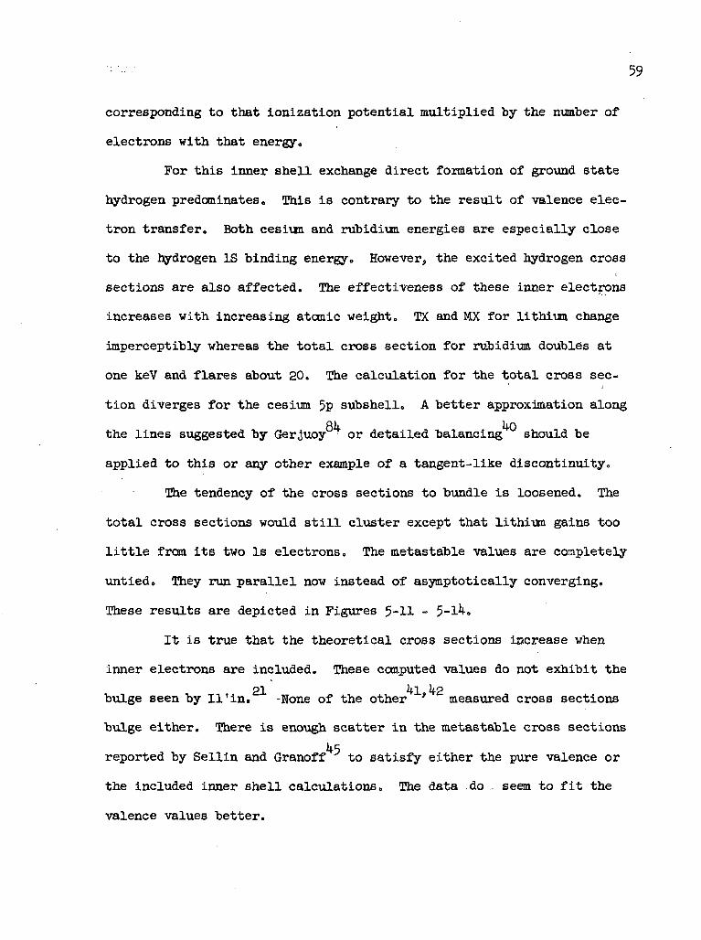
59
corresponding to that ionization potential multiplied by the number of
electrons with that energy.
For this inner shell exchange direct formation of ground state
hydrogen predominates. This is contrary to the result of valence elec-
tron transfer. Both cesium and rubidium, energies are especially close
to the hydrogen IS binding energy. However, the excited hydrogen cross
sections are also affected. The effectiveness of these inner electrons
increases with increasing atomic weight. TX and MX for lithium change
imperceptibly whereas the total cross section for rubidium doubles at
one keV and flares about 20. The calculation for the total cross sec-
tion diverges for the cesium 5p subshell. A better approximation along
Ak knthe lines suggested by Gerjuoy or detailed balancing should be
applied to this or any other example of a tangent-like discontinuity.
The tendency of the cross sections to bundle is loosened. The
total cross sections would still cluster except that lithium gains too
little from its two Is electrons. The metastable values are completely
untied. They run parallel now instead of asymptotically converging.
These results are depicted in Figures 5-H - 5-1 .
It is true that the theoretical cross sections increase when
inner electrons are included. These computed values do not exhibit the
21 4l 42bulge seen by II'in. -None of the other ' measured cross sections
bulge either. There is enough scatter in the metastable cross sections
U5reported by Sellin and Granoff to satisfy either the pure valence or
the included inner shell calculations. The data .do - seem to fit the
valence values better.
6o
5.1. 4. Detailed Balancing Results
Whenever the cross sections are discontiguous, they can still be
determined by using prescription (2, 35) « "For valence electron exchange
into the hydrogen ground state the weights are equal.
2The maximum contribution is less than k (-17) cm . The gap
between the lithium-sodium bundle and the K-Rb-Cs bundle again appears.
The ordering of the cross sections is the reverse of the TX values men-
tioned previously. The lithium cross section is now the largest, cesiumr"
smallest.
For inner shell transfer only the cesium value diverges. The6 *
electrons that form the (5p) shell are further divided energetically
into the 0-.J. (2 electrons at 13.1 eV) and Ojjj (h electrons at 11.4 eV)
subshellSo The ratios of the weights are U/2 and 8/2, respectively. o..Q
so calculated is shown in Figure 5»H-
Q ,(l,l) also misbehaves. It is calculated from a modified
version of Equation (2o26) where the binding energy is appropriately
changed. The weights are again equal. This value is used in computing
the curves of Figures 5-9 •- 5-10 -where It Is an upper 'bound to the
experimental values.
5«2. Determination of the Neutral Fraction Background
The major background gas is molecular hydrogen. It flows frcm
the source in the beam path at least until the middle of the magnet
chamber. There about one-half of the gas is removed by the 2" diffusion
pump. The most likely candidates for causing the zero target density
signal ( 8 ) for proton and molecular ion beams are

. +V
•* H •._>;. Hg
^V'V . V : '':'-. ' ' • . - . - • ' (5.7)
Q_ , Q£
Allison ' among others has ismstigated the first reaction. McClure
has measured the molecular hydrogen cross sections. The second reaction
above is much more likely in this energy range than a dissociative
collision into H or H+»
The background signals are fitted to the curares of Allison
(proton probe) and McClure (molecular hydrogen). They are plotted in
Figures 5-15 ° 5-l6« 8 is typically 0«OV0 It should be noted that the
potass ivm vapor data was taken earlier than the sodium. There seems to
be a larger background gas K value for the sodiisa target. Ion gauge
readings in the exchange chamber bear out this higher gas pressure for
the later runs. ;
Because of poor statistics all molecular hydrogen ion data were
averaged together,, Sheas data scatter much more than the comparable
proton values, nevertheless all path lengths-density (H) measurements are
consistent. Whenever the background fraction (3) is fitted to the above
mentioned cross sections with the methods of Appendix E, the normalization
constant is u itself. For the 26 cm path length between the magnet
chamber and the oven, this value and Equation (2.12) yield an average
pressure of about l(-4) Torr. Uncorrected exchange chamber ion gauge
readings were about half of this value „ The elbow (the magnet chamber)
gas pressure was about 001 Torr for 500 microns source pressure. Since
the molecular hydrogen density is higher towards the source, there is
good agreement between this derived value and

62
Table 5.5 lists the results of the above calculation. Potassium
served as the target earlier than sodium. Observed ion gauge determina-
tions aj© lower for the former as are the derived « values* By using
this data and the known cross sections, one can compute. thf rsasaaber .:," v-/-
of metastable atoms formed by collisions with the background hydrogen
5.3. The Metastable Hydrogen 2S State
5.3.I. Sources of Metastable Atoms
The metastable cross section for electron capotre (MX) has been
calculated from Equation (2.26)0 It is assumed that it is one quarter
of the value for capture into the first excited state, MX is displayed
for various targets in Figure 2*5., Cascade effects are important for the
total 28 population. The C channel contributes about 13 per cent to the
number formed (see Figure 2-8).
Collisions with hydrogen gas also contribute. The background gas
it values found in the preceding segment can be used to calculate the87initial metastable concentration. Van Zyl, Jaecks, Pretzer and Geballe '
report this cross section to be 6 (-17) cm . The background metastable27fraction is then 7 (-3). Bayfield claims it is 1 (-17). This reduces
the fraction to 1 (-3).
The attempted UV detector calibration of Section k ranks in
history with that famous success, Apollo XIII0 As the hydrogen pressure
increased, the counting rate decreased.'
Although the in situ calibration was a smashing failure, xi -
Equation (U.8) - can be estimated. Instead of the expected ratio of
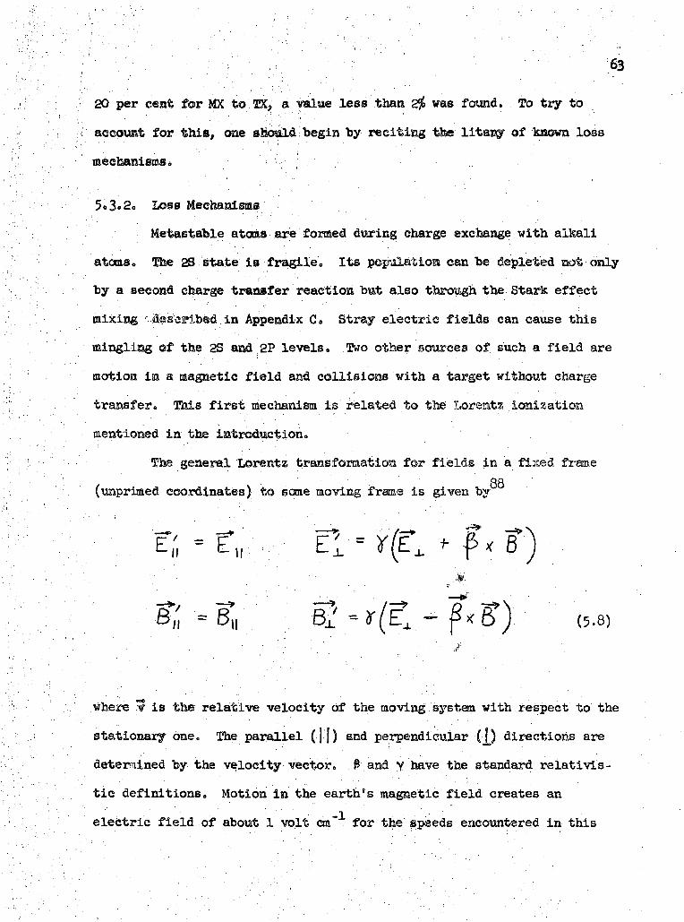
20 per cent for MX io'.lXj- a value less than 2$ was found. To try to
account for this, one should begin toy reciting the litany of Known loss
5<>3o2o Loss Mechanisms
Metas table atoms are formed during charge exchange with alkali
atoms, fhe 28 state is fragile. Its populatioa can "be depleted not only
by a second charge transfer reaction bw,t also through the Stark effect
mixing Seses'ib d in Appendix C« Stray electric fields can cause this
mingliffig ©f the 2S and 2P levels. Two other sources of such a field are
motion in a. magnetic field and collisions with a target without charge
transfer. This first mechanism is related to the Lorentz ionizatioa
mentioned in the introduction.
The general Lorentz trans formation for fields in a fixed frameQQ
(unprlmed coordinates) to some moving frame is given by
E.*;
(5.8)
where is the relative velocity of the movingsystem with respect to the
stationary one. The parallel (] j) and perpendicular •(•][) directions are
determined by the velocity vector. $ and y have the standard relativis-
tic definitions^ Motion in the earth's magnetic field creates an
electric field of about 1 volt cm" for the speeds encountered in this
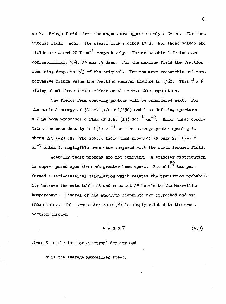
work. Fringe fields from the magnet are approximately 2 Gauss. The most
intense field near the einsel lens reaches 10 G. For these values the
fields are k and 20 V cm""1 respectively. The metastable lifetimes are
correspondingly 35 , 22 and .9 Usec. For the maximum field the fraction -
remaining drops to 2/3 of the original. For the more reasonable and more
pervasive fringe value the fraction removed shrinks to 1/60. This v x B
mixing should have little effect on the metastable population.
The fields from comoving protons will be considered next. For
the nominal energy of 30 keV (v/c » 1/150) and 1 cm defining apertures
-1 2a 2 MA beam possesses a flux of 1.25 (13) sec cm" . Under these condi-
tions the beam density is 6(k) cm"*0 and the average proton spacing is
about 2.5 (-2) cm. The static field thus produced is only 2.3 (~k) V
cm which is negligible even when compared with the earth induced field.
Actually these protons are not comoving. A velocity distribution89
is superimposed upon the much greater beam speed. Purcell has per-
formed a semi-classical calculation which relates the transition probabil-
ity between the metastable 2S and reso&ant 2P levels to the Maxwellian
temperature. Several of his numerous misprints are corrected and are
shown below. This transition rate (W) is simply related to the cross
section through
W = N 9 v (5.9)
where N is the ion (or electron) density and
v is the average Maxwellian speed.
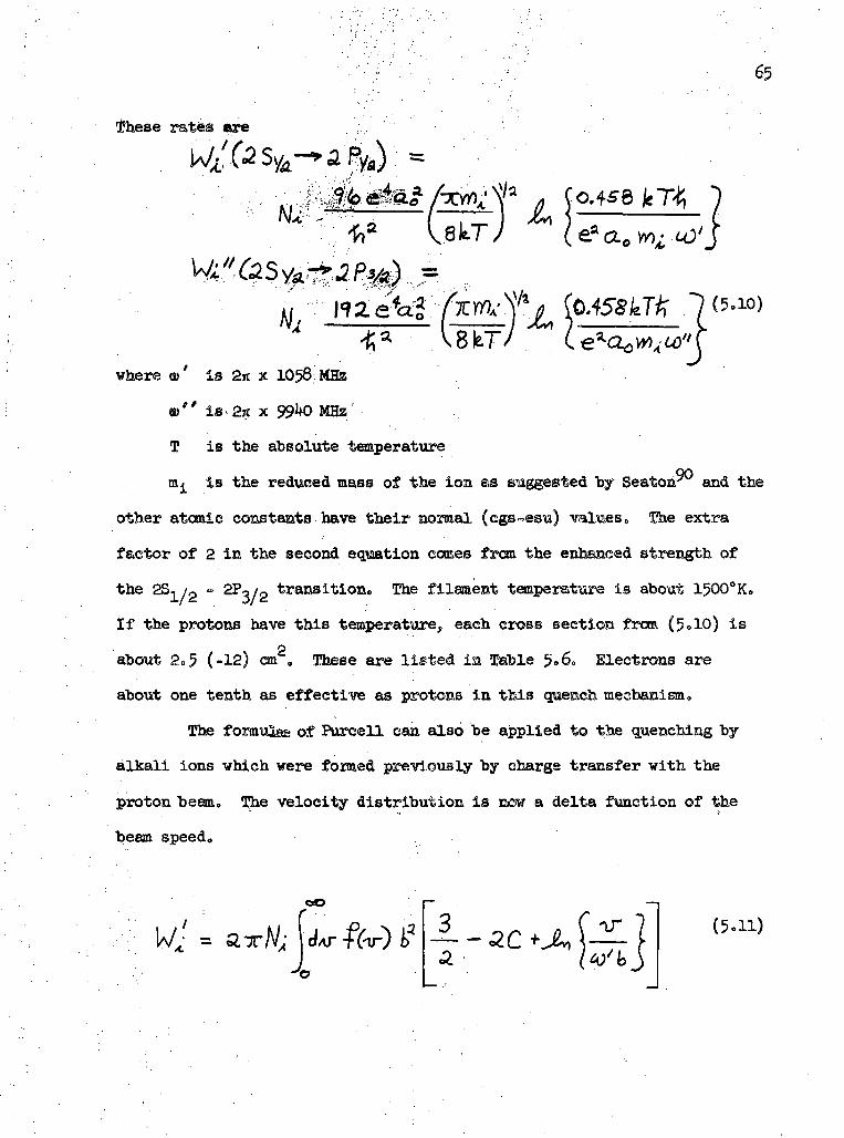
These ratfes are
,90
where w' is 2n x 1058 MHz
w" is> 2rt x 991+0 MHz '
T is the absolute temperature
m^ is the reduced mass of the ion as suggested by Seaton7V/ and the
other atomic constants have their normal (cgs-esu) values. The extra
factor of 2 in the second equation comes from the enhanced strength of
the 2S-L/2 - 2Po/p transition. The filament temperature is about 1500°Ke
If the protons have this temperature, each cross section from (5°10) isn
about 2«5 (-12) cm . These are listed ia Table 5->6. Electrons are
about one tenth as effective as protons in this quench mechanism«
The formulae of Purcell can also be applied to the quenching by
alkali ions which were formed previously by charge transfer with the
proton beam. The velocity distribution is now a delta function of the
beam speed.
(5.H)

•• ' . . . • ' '•/'( • • • " ' ' - ' i - ' •••••• . ' ; ; - ; - v / : . . . • ; . . • . ; 6612 e^u2 v ; '"• : /. '..-.-,. .;/• . .
C s 0.5771 (Euler's constant).
The cross sections so derived are shown in Table 5.7. Their sun isP 91roughly 1 (-13) cm » Wllcox and Lamb"7 have extended the Purcell
relations to 3S - 3P transitions. Since this S state decays by dipole
radiation, its lifetime is not noticeably affected.
l3ffiafi<SiMce& to being quenched by ionic impacts, the metastables
are also disturbed by molecular collisioas. The dipole-multipole inter
92action changes the internal state of the molecule as well, Gersten
has calculated these cross sections and has compared them with the
experimental results of Pite and coworkers. For their thermal beams
there is very good agreement between theory and observation. The cross
sections may be approximately written as
A+i / £+1 /3«*io
where g^ = 5/3 for I = 1 (dipole interaction), g s 56/ 5 for / » 2
(quadrupole) and the average is performed over the projectile speed.
93With the measured quadrupole moments of Bloom et alv and an average
speed of 8 (5) cm sec" (1/3 eV) all values agree to within; about 25
per cent. Incidently, the cross section for C02* which has not been
measured, is calculated to be 3.5 (-1 ). This is somewhat larger than
the observed values for Np, Og and BU but is one sixth the water vapor
67
result. When this calculation is extended to kilovolt energies, the
cross sections are still considerable - about 5 square angstroms.
The background gases that could quench the 2S atoms in this
manner are primarily molecular hydrogen, air, water vapor and hydro-
carbons from the p\mp. Water is the most efficient of the metastable
destroyers that have been measured but it should be a minor constituent
due to trapping by the cold bucket around the oven. Hydrocarbons
9typically exhibit a dipole moment of 2 (-18) esu. Since this is
nearly the value for HO, hydrocarbons should behave like water vapor.
Molecular hydrogen should be the primary target. It is the most abundant
background gas. The following cross sections are taken from Table 5«8
for a 10 keV proton beam: o(W2) « 6 (-16), e(02) = k (-16),
o(H ) = (-16), e(HgO) = 3 (-15). For measured hydrogen densities the
poptilation change will be a few per cent.
Sellin's 3 component fit has yielded a total depletion cross
2 kksection of 2 (-15) cm at 15 keV. Equation (5.13) for H quenching
gives 2. (-16). This suggests that removal of the metastables by
ionization may be very important.
Other investigations in this energy range have been conducted
95-97recently. Three loss mechanisms have been considered. Electron
loss by stripping rather than by charge transfer has been studied. The
two other destruction mechanisms are de-excitation and formation of H"
98by electron capture. Bates and Walker have calculated the cross sec-
95tion for ionization. The results of Dose, Meyer and Salzmann for
nitrogen and water vapor quenchers may indicate H" formation is important
below 5 keV. The combination of Gersten and Bates and Walker calcula-
tions adequately describes the high energy region, however,,
68
96The total quenching cross sections for hydrogen, nitrogen, and
95 2water vapor are about 1 (-15) cm . The ionization cross sections for
Hg and the noble gases ° seem to be approximately 3 (-16). Cesium"' at
2.5 keV has this same general value.
5«3»3« Tentative Solution to the Case of the Missing Metastables
As the calculations of Section 5«3«2 show, large quenching cross
sections do exist. The problem is how to couple a large cross section
with an abundant metastable destroyer. There are not enough protons for
the Purcell values to be effective. The number of alkali ions present
is also too low. For total conversion of protons into neutrals and
complete retention of the resulting ionized alkalis there will be only
2.5 (9) ions per cubic centimeter at day's end. Hydrogen is present in
larger quantities but its cross section is some 4 orders of magnitude
smaller. Clearly something more is needed.
If the charge transfer process is viewed as resulting from the
presence of an external electric field, then a possible solution appears.
Assune that this field is so intense that the 2S and 2P states are
thoroughly mixed. After a few nanoseconds the metastable state will be
depleted. In the time it takes to reach the UV detector the more highly
excited states can decay into the 2S state. The metastable ratio will
then be about 1$ which is the observed value,
2*4-Donnally says 0.3 per cent of his protons were converted intoP
metastables. For his published value of 4 (-15) cm which may be|i -l _p
somewhat low one deduces H to be less than 1 (12) cm" . Sellin in his
H studies operated near 1.5 (15) cm with his 10.16 cm oven. The meta-
-18 2stable formation cross section there was a few times 10 cm which is
69
much less than the expected alkali values. The oven used in the present
experiment was 16 cm long. As the metastable data of Figures 5-17 and
5-l8 show, the present TT values are larger than those of Donnally but
smaller than those of Sellin,
Sellin built a model consisting of three beam components:
protons, ground state hydrogen atoms, and metastable atoms. Using equa-
tions similar to those in Appendix A for three charge states, he was able
to fit the metastable signal as a function of E^ density. The resulting
curve looks like a question mark lying on its side. There is an initial
linear region. This is followed by a peak and then the signal decreases
toward a lower asymptote. This is totally consistent with the observed
sodium data. Curvature is evident in Figure 5-18. Other data show the
peaking and the subsequent decline.
There seem to be two different effects operating here. The
metastables are being quenched by the alkali target. The counting rateo
is linear below a soditm density of about 5 (12) cm « Then the rate
becomes at least a quadratic function of density. The background signal
is linear throughout. This layman alpha probably comes from decay of the
2P states. The resonant levels are filled from higher ones. The cross
sections for populating these states are much smaller than MX. The initial
populations will be linearly dependent on the target density. Hence this
background signal will be, too<>
The 20 keV data can be interpreted as a two state picture, for
example. The metastable creation cross section is 5 times the background
value. It should be more like 100 times as great. The sum of MX and the .
loss value is about 27 (-16) cm . Similar values can be deduced from the

70
16 keV data of Figure 5-17« As Sellin has shown, the 3 component model
is needed to explain the variation of metastable fraction with density.
It is difficult to estimate the depletion cross sections for this reason.
A second effect is the reduction of counting rates. If the
counter efficiency is known fairly well, another quenching mechanism is
probably needed. A guess at the size of this cross section is about
1/3" or 2 (-1*0 cm2, which is rather large. Sellin does need a quench
cross section of about 2 (-15) for a much larger path length-density
product and lower formation rate, however.
If the formation field is so strong as to ravish the 2S state so
completely, it may not affect any other state. All other excited levels
can decay through dipole transitions. Such a field will mix them too but
not change their populations so drastically. The idea of the populations
being related to the statistical weights would still be valid for all but
the metastable state.
5.U. Excited Alkali Atoms
The viewing port in the exchange chamber overlooks the front of
the oven. Through the plexiglass brightly shines akaline light. With
sodium in the oven, an intense yellow light is seen. Protons colliding
with potassium atoms produce a washy blue color. The sodium radiation
comes from the famous D lines ( 5895.93, 5889.96). These arise from the
transitions 3 J? - 3 S. The corresponding lines in potassium (4T1 - k S)
lie in the infrared at K\j6kk.9k, 7699.01A. The 5 - 42S transitions
are visible and are blue (XX40H.14, 4oVf.20). These states should
not be as heavily populated as the lower lying P states. Consequently

' 7 1
this blue radiation should not be as intense as the infrared potassium
light or, by extension, the sodiua D lines. In fact, the blue light is
much weaker than the yellow. Since two different energy levels are
populated, one infers that most (if not all) alkali states are populated
by the proton interaction. This result also appears in the calculation of
Q in Section 2o*v.2» Hence, charge exchange reactions between pro-
tons and alkali atoms create excited alkali atoms as well as excited
hydrogen atoms.
ft has been calculated for charge transfer with excited alkalis,
Figure 5,19 shows the cross section for electron capture from the first
excited state for both sodiua and potassium,, This cross section is twice
that with ground state targets. Metastable formation is much less. The
density of such excited targets is very small however. It can be calcu-
lated by equating the msaber of atoms that decay per unit time and unit
volxme to the msnber formed from the proton beam per second per unit beam
per unit area. It follows that
n qA
where n* is the mmber density of excited atoms,
n is the alkali density,
I Is the beam current,
q. is the proton charge,
A is the area of the beam,
9 is the cross section for making the excited atoms,
T is the lifetime of the state. \

For reasonable values for these quantities, the ratio i* only 1 (-8),
The D lines were also seen for Hp • Even if the excitation (without
electron transfer) cross section is much larger than 1 (-l ), he ratio
will still be small for believable values.

6.0. CONCLUSIONS
6.1. Overview
In this work the interactions between hydrogen ions and alkali
atoms are studied. The proton study may "be divided conveniently into
three main parts. The first is the experimental determination of the
total electron capture and loss cross sections (ff and 0Q,) for
potassium and sodivm. The proton energy ranges between h and 30 keV,
The second major point is the modification of Gryzinski theory for
charge exchange between protons and alkalis. Predictions are made for
both the total charge exchange cross section ( Q ) and the cross
section for exchange into just the metastable hydrogen 2Si state.
Comparisons are made between these values and measured ones. In this
way the observations of several groups (including this one) can be
systematized. The investigation of Lyman alpha radiation from meta-
stable hydrogen atoms is the third theme.
Several minor points are also covered in the present work. A
fast survey of cross sections has been run using molecular hydrogen ions
in place of protons. These seem to be the only measurements in the 10 -
30 keV range.. Collisions between both ions and hydrogen gas create a
background atomic hydrogen beam. The fraction so produced is directly
proportional to known cross sections. Proton collisions with alkali atoms
excite the target atoms. As they decay, they emit copiously. During the
study of the hydrogen 2S state, the sharp angular sensitivity of the
molecular.oxygen filter has been calculated. These various matters will
now be examined in more detail. ,
73

6.2. Proton Beam '
The measured proton data are consistent with both the sparse
21experimental points of II'in, Oparin, Solov'ev and Federenko and the
modified Gryzinski calculations of Section 2. The total electron
capture cross sections (0,o) agrees with the theoretical charge exchange
cross section ( Q ) to within a scale factor, ff for potassium is10 01 10
1. 65 times the computed value for charge exchange into all excited
hydrogen states. The test value for the sodium multiplicative factorIi2
is 1. 38. Elsewhere1, Schlachter et al. report C, Q for cesium, which is
1.31 times larger than the theoretical result here. The measured values
for a1Q are thus within a factor of two of the exchange cross section
(inQm). It appears that the major component of ff is _* as has
been assumed in Section 2.
The measured cross sections (ff ) for both sodium and potassium
agree generally with those of II'in. For potassium the values found here
agree very well at low energy but are much lower near 30 keV. The quoted
Inresults of Sctaelzbach are much lower than either the present data or :;
the Russian values. The discrepancy is roughly a factor of four. This
is probably due to difficulty in determining the oven density. However,
all three results exhibit the same shape above 5 keV.
The sodium target data agrees well with II'in. The flaring that
appears in his potassium cross sections does not occur here for sodium.
The general shape of the curves agrees with the Gryzinski form given by
(2.30). The systematic difference between the two curves (the "gap")
is distinct in the present work but is much less noticeable in Il'in's
T5
results. Even there, however, potassiun cross sections are always larger
than sodium values. Here, if anything, the gap is too large.
The asymptotic values also agree well. The single point of II 'in
almost coincides with the present measurement for K. The values of
Schmelzbach are consistently lower. For sodium the present data lie
"below that of II 'in. When these results are combined with those of
Schlachter,i one sees that F • for alkalis is quite consistent. Belowv
ten kilo-volts the maximxm neutral fraction is nearly unity. Then ito
declines monotonically. Near 20 keV the ratio "becomes one half. F «•
falls to 0.25 near 30 keV.
6.3. H2 . Beam
The cross sections for the molecular hydrogen ion are uniformly
larger than those of the proton probe. C10 for potass ivm seems to be
much larger than ff,0 for sodium. The reason for the apparent factor of
4 difference is unknown. The neutral fraction is also larger for Hp
than for H at the same energy.
6.1*-. H(2S)
Since the in situ calibration of the layman alpha detector was a
failure, it is necessary to estimate the counter efficiency. Assuming
this is known to about a factor of 2, one needs to invoke a powerful
quenching device to destroy the metastables formed by direct exchange.o
The cross section for this annihilation is approximately 2 (-1*0 cm .
This value is compatible with known depletion values. A new mechanism
seems to be required; the standard ones are not powerful enough. Sodium
76
quenching of the 2S atoms is evident. This cross section seems to be
out
-16
n
about 2 (-15) cm , The predicted creation value is only a few times
10
The modified Gryzinski calculation indicates that all metastable
cross sections will be nearly equal above 10 keV. This has been
U5observed. Also the ratio of the metastable to the total cross section
should be approximately constant at ten per cent. No data are available
on this.
Metastable atoms are formed by charge exchange directly into the
state. Cascading from higher levels will also populate the 2S state. If
all mj substates are filled, this increases the population by about
13 per cent. Half of these decays occur within 10 nsec of their birth.
If only S state atoms are created, the cascade effect is much smaller
and much slower. The population enhancement is 2%$ after \ msec. Half
of these decays occur within 200 nsec after they have been formed,
Such indirectly formed metastable atoms seem to be the only metastables
observed in this experiment.
6.5. General Remarks
Equation (2.30) describes quite well the cross sections for
protons interacting with the alkalis. If inner shell electrons are
included in the calculations, the predictions are not as accurate. Both
a and e (2S) are noticeably affected. The data does not support this
inclusion. In medical argot, it is "contraindicated".o
The Born approximation as calculated by Bates and Dalgarno also
predicts large cross sections. Unlike the classical calculation, the
77
Born predicts that ground state formation overwhelms metastable creation
above 25 keV. The Gryzinski calculation, when modified "by detailed
balancing, relegates the ground state to a continuing role as a minor
constituent.
There are experimental anamolies as well. For example, the
k5metastable cross section found by Sellin exceeds the total valve found
by Schlachter, Sellin does normalize his results to the cesiun cross
sections measured by II'in. Schlachter's results seem higher than thejig
Russian values. Spiess has verified these higher values near one
kilovolt. It seems that Il'in's experimental shapes may not be quite
right. His results do show the proper ordering, however. The largest
cross section does belong to cesitm and the smallest to lithiun. This
result is predicted by the calculations of Section 2.
The question of relative population of the sublevels is still
unanswered. The metastable cross sections reported so far are too large.
Even if the s electron of a ground state alkali is transferred to a
hydrogen s state during the charge exchange collision, the measurements
remain high. Because of decay from higher levels into the metastable 2SjL
state of hydrogen, the effective cross section for producing these meta-
stables will be larger than the direct exchange value (the o channel).
This augmentation will be time dependent. Its exact magnitude and time
variation depends strongly on the model of relative hydrogenic populations
used. For the "all state" model the cross section will be increased 13$
in about 20 nsec. On the other hand, the s state model reduces this en-
hancement to about 2 per cent. This requires nearly one half of one
microsecond. Probably experimental transit times between the metastable
source and its detector are tens of nanoseconds.
Counterbalancing this enhancement of measured cross sections by
decay is the severe angular selectivity of the commonly used iodine UV
detector and its oxygen filter. The filter properties are strongly
energy dependent. For the tens of kilovolt energy in this experiment
and the small (~ 5$) geometrical apertures, the Lyman alpha cross section
has been reduced "by about 20 per cent. Scattered light will be rejected
by the filter as the beam energy is increased. Apparently such reflected
light artificially increases many measurements of the metastable cross
section.
O10 for protons on alkalis agrees fairly well between the various
experimental groups and modified Gryzinski theory, but the metastable
cross sections disagree with both this theory and the various groups.
Below 30 keV cr10 is probably known to within a factor of two for all
alkali vapor targets. The metastable cross section even for cesrum is
still uncertain to an order of magnitude.
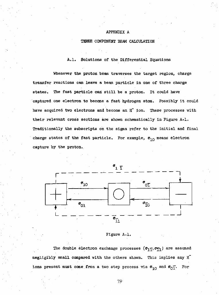
APPENDIX A
THREE COMPONENT BEAM CALCULATION
A.I. Solutions of the Differential Equations
Whenever the proton beam traverses the target region, charge
transfer reactions can leave a beam particle in one of three charge
states. The fast particle can still be a proton. It could have
captured one electron to become a fast hydrogen atom. Possibly it could
have acquired two electrons and become an H~ ion. These processes with
their relevant cross sections are shown schematically in Figure A-l.
Traditionally the subscripts on the sigma refer to the initial and final
charge states of the fast particle. For example, CIQ means electron
capture by the proton.
*iTr 1
i_-(-
_« 0
e—11
Figure A-l.
The double electron exchange processes (oiX><7Tl^ are assume(^
negligibly small compared with the others shown. This implies any H~
ions present must come from a two step process via ff,Q and OQ . For
is-

- • • • •example, Schlacter et al. measured 9, £ tor cesium for 2-15 keV. He
found it varied from 3.7 (-1?) to 5.2 (-18) cm2. Schaelzbach and co-
in. ' •workers also investigated this cross section for protons on potassiua.
In the energy range of 2.5 to 22 keV it declined monotonically from about
2 (-1?) to 1 (-18) cm20
The simplified differential equations relating the various
beam components may be written as
= -<57o
(Al)
(55-r r
where D = -r— (D is the differential operator)QTT
n a n(x) x (n is the target density at x)
tot
Naturally since the equations are written in terms of fractions,
F° + P+ + F" = 1 . (A2)
For this work the ion fraction of interest is the so-called
"neutral fraction" (F°), A straightforward but tedious method of solving
the system of equations for Just F° is to differentiate the second of
(Al), substitute for the various derivatives and eliminate F". A more
powerful and elegant method is given in Section 2. Either way after seme
algebraic manipulations the following equation emerges;

D*(A3)
The solution is
F^^Ae-^VBe-^ +C (M)
where • . . '.; • . ..;•.•'.'• • ".
^ == p •»• Q (A5)
(A6)
o^ Oor) t (AT)
o- (A3)
• (A9)
In order to evaluate A and B let
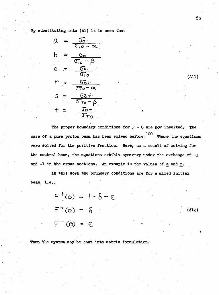
62
By substituting into (Al) it is seen that
a - $01Q/o -06
b =_
£ - (TodT,
r = gordTo (A11)
(Tfo-ocS = _
t =
The proper bovmdary conditions for n = 0 are now inserted. The
100case of a pure proton beam has been solved before. There the equations
were solved for the positive fraction. Here, as a result of solving for
the neutral beam, the equations exhibit symmetry under the exchange of +1
and -1 in the cross sections. An example is the values of a and r.
In this work the boundary conditions are for a mixed initial
beam, i.e.,
= l-S-e
F°.CoV=- S
Then the system may be cast into matrix formulation.;
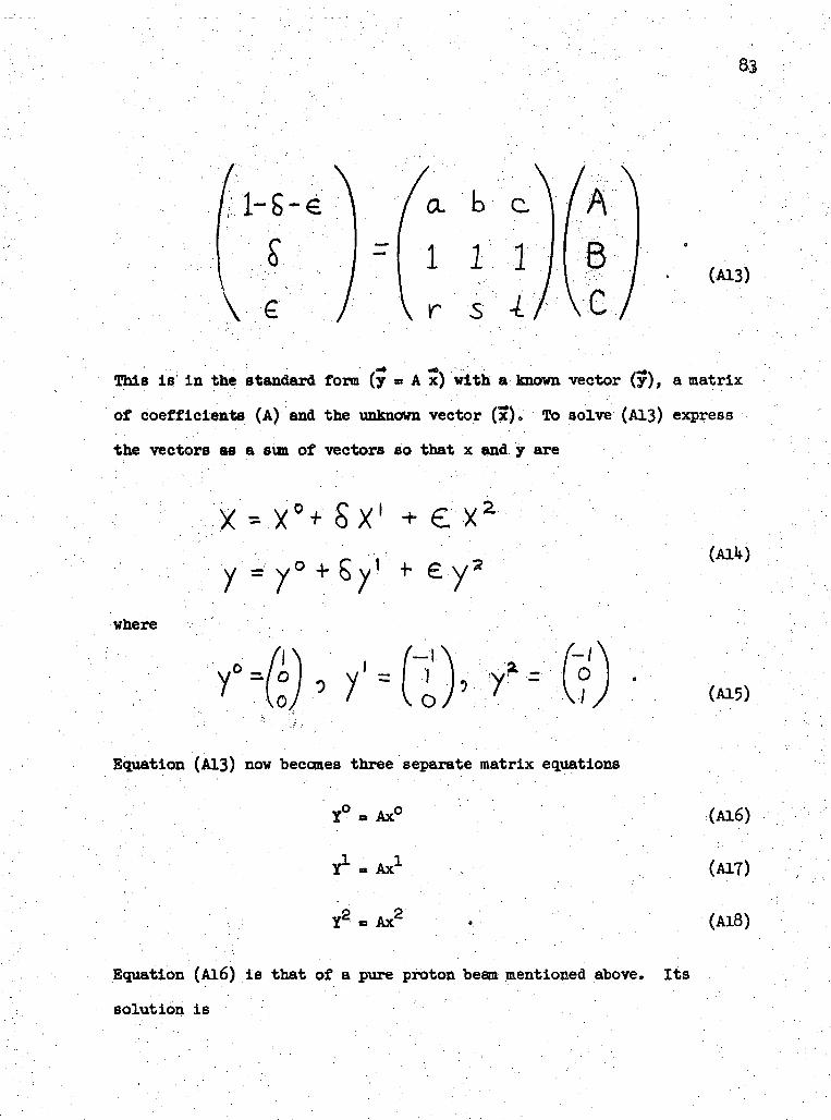
,1-S-e\ Y
1 11
\ r s 47 Ve/(A13)
• ' «* «0 . " ' • • ' ' ' • ' M*
This is in the standard form (y « A x) with a known vector (y), a matrix
of coefficients (A) and the unknown vector (x). To solve (A13) express
the vectors aa a sun of vectors so that x and y are
Sx1 + ex= ° 4-y = y
where
(A15)
Equation (A13) now becomes three separate matrix equations
Ax
Y1»Ax1
Y2 - Ax2
Equation (Al6) is that of a pure proton beam mentioned above. Its
solution is
(A16)
(AIT)
(A18)

B° >
C°r
A
V-A
S-r
where
A = deta c
i I ir 3 t
The solutions of (A17) and (Al8) are respectively
/..=• A
A
C1 = A
B2 =
Ca =
A
C - PL -t- i: - rA
r~s •f-.-o.A
(A19)
(A20)
(A21)
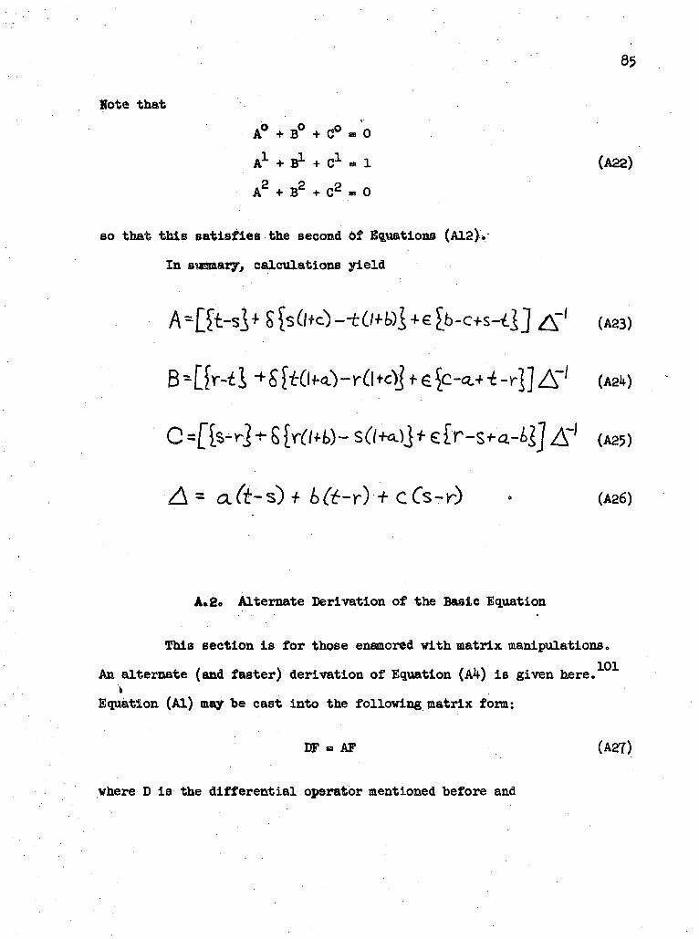
85
Note that
A°
+ B1 + C1 « 1 (A22)
A2 + B2 + C2 « 0
so that this satisfies the second of Equations (A12)v
In swaary, calculations yield
A"" (A23)
-yj A'1 (A25)
A = aft-s) + tft-r) -^ cCs-n) • (A26)
A.2o Alternate Derivation of the Basic Equation
This section is for those enamored with matrix manipulations.
An alternate (and faster) derivation of Equation (AU) is given here.'& .
Equation (Al) may be cast into the following matrix form:
DP B AF (A27)
where D is the differential operator mentioned before and

86
"P" —
(A28)
A -=o
Go"/i+
GOT
0
(AS9)
Now let
P o VG (A30)
where the matrix V is so chosen that it is independent of and G and
V^AV is a diagonal matrix. Then (A30) becomes
DQ » V^AVG (A3D
,thLet a. be the i n eigenvalue of A, Then each component of Equation (A3l)
can be easily integrated to yield equations of the form
(A32)
Use (A30) to solve for F. Then the i component of the F vector, which
is some charge component, satisfies

In the problem considered here
£ J Ao-
(A33)
The eigenvalues of A satisfy
5 1" o^ _L o - - > _ . v* I = r\L Q T £ p 4 ' + f J U (A35)
where p is given by (A?) and Y by (A9). Hence
(A36)
and Equation (A33) is Just (A4).
i
A.3. Exact Evaluation of the Coefficients
It is usually assumed that the thick target asymptote is very
nearly that of the two charge system, i.e.,
(A37)
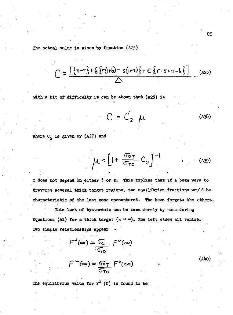
The actual value Is given by Equation (A25)
(A25)
With a bit of difficulty it can be shown that (A25) is
C = C U (A3B)U
where Cg is given by (A37) and
C does not depend on either 6 or «<, This Implies that if a beam were to
traverse several thick target regions, the equilibrium fractions would be
characteristic of the last zone encountered „ The beam forgets the others,
This lack of hysteresis can be seen merely by considering
Equations (Al) for a thick target (« •* •»)«, The left sides all vanish.
Two simple relationships appear -
The equilibrixan value for P° (C) is found to be

This is another fora of (A38), It is independent of the boundary
conditions at zero density. Also the second of Equations (Ato) becomes
1 - Ifc (Ate)
Typical values for'a tb /target are F(») « % and F"(«) ~ 1/100,
The ratio of the cross sections in the definition of p is quite small,
The two component system should have asymptotes very close to those of
the 3 component system.
The coefficients of the exponentials do depend on 6 and «0
Equations (A23) and (A2 ) become
/- s/ *•§& l-* 5kz
The superscripted terms are given by (A19)o They become
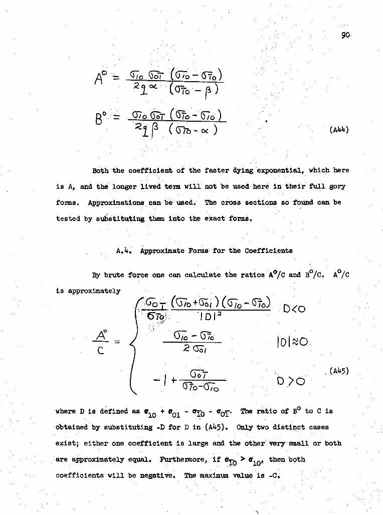
9"0
/p. AZ ^UIQ - a
((T/b-cx )
Both the coefficient of the faster dying exponential, which here
is A, and the longer lived term will not be used here in their full gory
forms. Approximations can be used. The cross sections so found can be
tested by substituting them into the exact forms.
A. 14-. Approximate Forms for the Coefficients
By brute force one can calculate the ratios A°/C and B°/C. A°/C
is approximately/*<TI _ f rrr j.f\~ ^ f r\~~ _ (\~ \
D<o
where D is defined as o + OQ. - O^Q - OQQ-. The ratio of B° to C is
obtained by substituting -D for D in (A 5), Only two distinct cases
exist; either one coefficient is large and the other very small or both
are approximately equal* Furthermore, if ew > 0,0, then both
coefficients will be negative. The maximum value is -C.

Since the two charge state should be a good approximation, (A6)
can be written in the nice form
where
(AW
The first term in (A T) is Just (2,10), the two component equation. The
H" fraction should influence the correction (AVf Bottom) strongly.
Definitions (A5) . - (A9) indicate that P should be affected more by H"
than a,
There should be enough information in the difference expression
(A 7 Bottom) to determine two more cross sections (er_ and 0Q»>)° Three
things are particularly useful in this correction. The low density slope
of the curve, its total area, and the position of the maximum can be
conveniently used to find the negative ion cross sections. Any two of
these will be sufficient for CJQ and OQ , The third one can be used to
verify the values. The peak could be easily missed. This one will be
the check. The slope (mo), the area (S),, and the peak position
are given by
B- <<= 2? 6-
The peak position can be approximated as I/a.

The first approximation (2.9) yields <», S and C. The ratio of
the area to the slope can then be used to find P. The slope gives B
Immediately. The boundary conditions fix A. The coefficient C is just
the asymptote given by (2«1 )<> The two known cross sections (ff o and
OQ ) are substituted into Equation (A9) and then (A?) yields all fow cross
sections. This can be iterated to give the best values for ev-Q and CTQY°
As a check the position of the maximun difference (u ) can be
calculatede Whenever an four values are known, the fit to (A6) can be
compared with the data.
The two charge state predicts a simple linear equation for the.» . '
neutral fraction behavior near zero density. For small n Equation
becomes
This can be rewritten as
j
where
(A51)
The first of (A$l) can be approximated as

/-
1=
jn . >- ™""*«.r.i <J5 1.1 <57o-ff7o
V.
C*D [,2-A.(57o I1
•far\ p.UroJ 2
? -o3 1D|
GOT 7^7b-G70 J |D |>o
|D|*0
Equation (A50) is to be compared with
I- 807o
(A52)
7C ' (2.12)
The terms are similar but their near equality depends on a fortuitous set
of cross section values, i.e., D small.
A. 5. Hydrogen Molecular Ion as the Probe
In addition to the proton beam discussed above, runs were made
vlth the Hp beam on both sodium and potassium- The interpretation of
this data is more difficult than for proton beams.
In the following reactions X is the target alkali atom* The
capital letter refers to the cross section for the reaction proceeding
left to right. The corresponding small letter is for the reverse •
reaction. For example, OQ here is ff,0 above and ff_ is the electron
capture cross section. This system is somewhat simplified for negative
ion formation is not considered. There is also no distinction between

the various possible excited and ground states,,
H *H + X"
- (A53)
H2 X
H +/ =
In the same manaer as Appendix A,2 the differential equations
for this set of charge transfer reactions become
DO = MG
where D is the differential operator
G is the vector of specie fractions
M is the matrix of cross sections.
In analogy to the earlier definitions the specie fractions are
G° .
-*"'•+ 4
Hp + Hp + H + H
(A55)
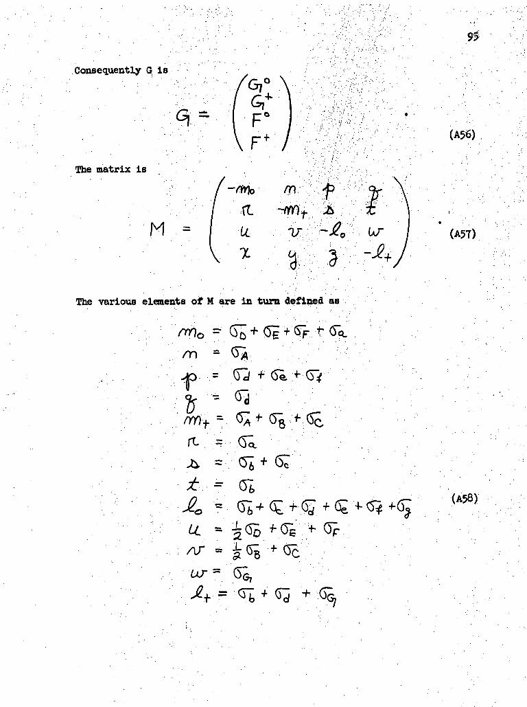
Consequently G Is
The matrix is
n
M - l LL v -J o u-x a-The various elements of M are in turn defined as
t (TC/n -
fIft. =
6;
AT =
(A56)
(A57)
(A58)

96
Note that again
0° + + F « 1
DG° + DO •*• DP + DF = 0(A59)
The factors in the exponents of the solution obey
det M -1 - O (A60)
After some manipulation the following fourth order equation emerges:
u r*f \(A6l)
where
R =•
a

os -
- '
It
crose section
— <- —MG * 2
s tfc • U.
V-
(A62)
(A63)
*2
H

The difficulties with the hydrogen molecular ion beam should now
be obvious. There are IV cross sections to be measured and four beam
components. Each component will be a complicated function of n: three
exponentials and a constant. This experiment measures only the total
neutral flux. The ratio of neutral flux to total flux (R) is
where x iB the fraction of the hydrogen atoms reaching the detector. If
the dissociation products gain energy from the interaction with the
target, X should be nearly zero.
For linear data runs (n small) only single scattering reactions
are important. Then
Ff =
F° =R r
If cr. and ff are the dominant cross sections, then the hydrogenA ft • .
ion components behave as the proton ones did above in Sections 2,2.

APPENDIX B
TRANSITION PROBABILITIES
In Section 2.5 the equations for the time dependent hydrogen
level populations were derived. They depend upon the Einstein A
coefficients. It was discovered that all substates through n » 12 were
needed. Various groups 60,102 have compiled these coefficients through
n m 6. Hence it was necessary to compute the rest. A large number of
radial hydrogenic integrals have been calculated. ' These were
used to determine the required probabilities* The coefficients are
related to these integrals through
A fl>y. '.*')"f
(M.)
where
Jg -for J?>Ji
Four digit values were used for the integrals. The resulting
coefficients were then verified by comparison with existing values. It
was then discovered that a nunber of mistakes appear in Condon and
]Q2Shortley. They are listed in Table Bl» The average transition probabil-
ity is defined by
99.
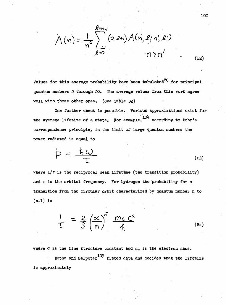
100
(B2)
Values for this average probability have been tabulated"0 for principal
quantum numbers 2 through 20. The average values from this work agree
well with those other ones. (See Table B2)
One further check is possible. Various approximations exist forIQl*.
the average lifetime of a state. For example, according to Bohr's
correspondence principle, in the limit of large quantum nuabers the
power radiated is equal to
=
' T (B3)
where 1/T is the reciprocal mean lifetime (the transition probability)
and to is the orbital frequency. For hydrogen the probability for a
transition from the circular orbit characterized by quantum number n to
(n-1) is
me.T 3 U 7 xK (*)
where o is the fine structure constant and me is the electron mass.
Bethe and Salpeter fitted data and decided that the lifetime
is approximately
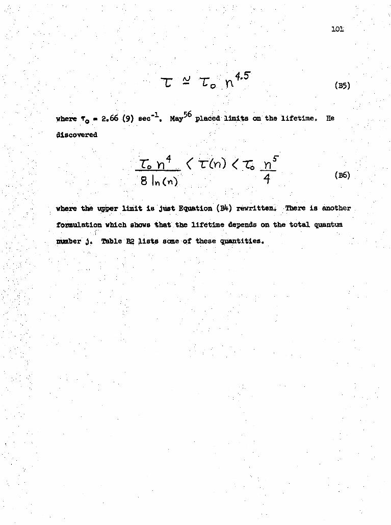
ioi
AJ ~r- . T*T A ~r- . T*- To ft (B5)
where To » 2.66 (9) sec"1, May^ placed limits on the lifetime. He
discovered
Q /o k(«
where the upper limit is Just Equation (B>t) rewritten There is another
f emulation which shows that the lifetime depends on the total guantua./ • . '
msober J, Table B2 lists seme of these q,uantities.

APPENDIX C
CALCULATION OF THE METASTABLE LIFETIME
The lifetime of the metastable 2S, level of hydrogen has been56-59,106,107 10,31,103
investigated both theoretically and experimentally
Under the influence of a weak electric field the Stark effect mixes the
metastable state with the resonant 2P levels. It is assumed that the
field is so weak that only the n = 2 levels mix together. This implies
any splitting is comparable to the 2P doublet splitting (about k-5 |ieV)
but is much less than the separation of the n » 2 and n = 3 levels (on
the order of 1 eV), This perturbation is
hg = -eEz = -eE r cos9 . (Cl)
Since h is an odd parity function of 9, the only nonvanishing
matrix elements are those between states of different parity. Farther-
more hs does not depend upon either the angle cp or the spin. The only
states that are mixed are those that obey Ams = 0 and Am_ = 0.v A IS
For simplicity assume the unperturbed Hamiltonian exactly selects
the 2P,, /p energy. This is taken as the zero energy point. It is con-
venient to rename the states so that "a" refers to the 2S. state, "b" to
2P, and "c" to the mixing 2Po/2 states. The unmixed states will be
designated "r" and the "g" state is the 1S^ ground state. The behavior
of the four excited states as the electric field strength varies is
depicted in Figure C-l. Separation energy is measured in millikaysers
[lK = 1 cm] with respect to the "r" state. Similarly, Figure C-2 shows
the change in the "a" or metastable state as a function of field strength.
In this representation the Hamiltonian M, which satisfies the
standard eigenvalue equation, can be broken into unperturbed and
102
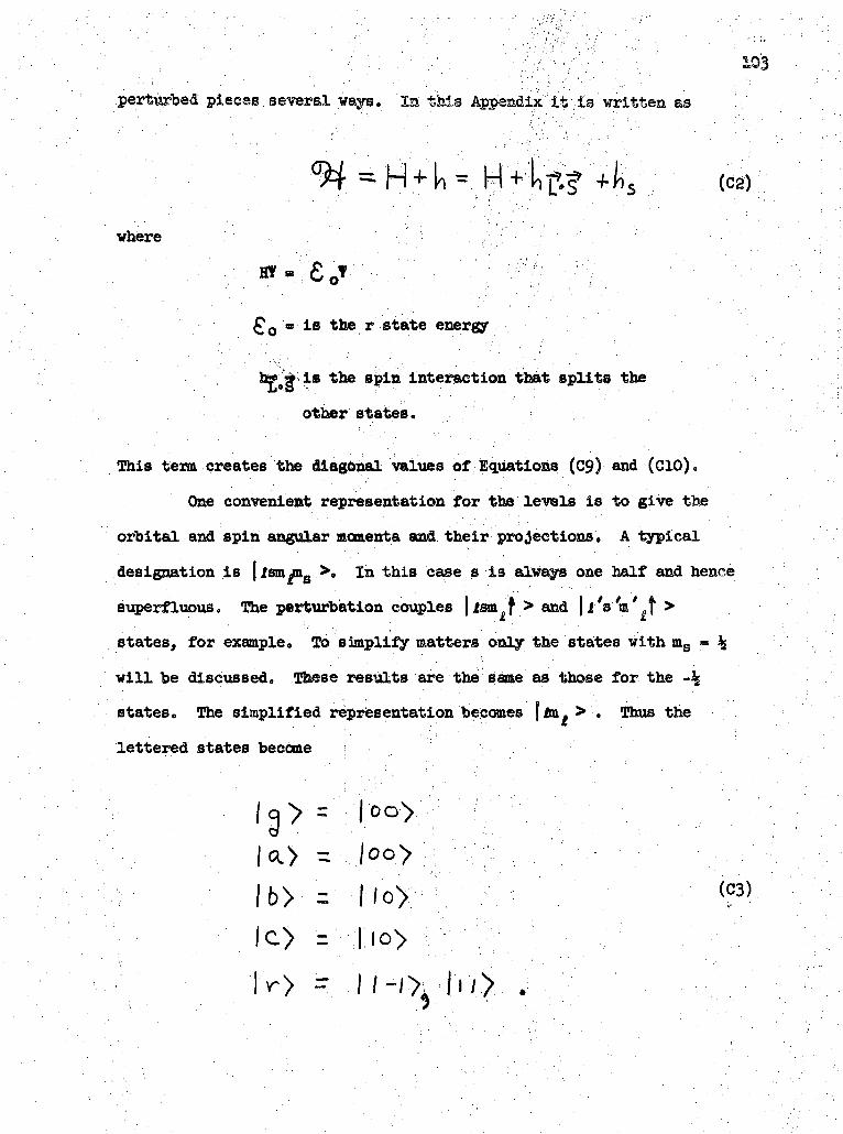
perturbed pieces several ways . la this Appendix/it .is written as
where
£o » is the r state energy
ha> 3 is the spin interaction that splits the• • il*-B "'•• . • ; ' " . ' ' . ' • • ' ' ' . . • • •
other states.
This term creates the diagonal values of Equations (C9) and (CIO),
One convenient representation for the levels is to give the
orbital and spin angular momenta and their projections. A typical
designation is |jsmjn8 >. In this case s is always one half and hence
superfluous. The perturbation couples \tsta. f > and | j's'm' f >
States, for example. To simplify matters only the states with ms = %
will "tie discussed. These results are the same as those for the -%
states. The simplified representation becomes fto. > . Thus the
lettered states become ;
- |oo>

In order to evaluate the matrix elements, the following relation-
ships are useful; ;
fTnr'
= a
A typical matrix element to be considered is < c/a >. For the
Schrodinger hydrogen atom this is
= -eEfdr e"4 (o)%
Y,,o
Equation (C5) can be evaluated with the aid of (C ) as
<ck> = (06)
where
= fT.eEct, (C7)
Similarly
/( '^V = b . (cs)
The quantity a is the first Bohr radius. Its numerical value is ,529
(-8) cm. Again it should be pointed out that throughout this work the
notation D(P) means D x 10 *

105
When the fine structure is taken into account, the total perturbation
matrix becomes
(C9)
where hi. » h?.a + h . In (C9) all energies are measured with respect tov J-J t* g •. ^ • .
the energy of the unmixed states (( Q)" ^ a is tlxe energy of state "a"
with respect to "r" and C^ the energy of "b". £ a and Q b are both
negative. If the 2P / state is neglected, the reduced perturbation
matrix becomes
Q,f \ 0
(CIO)
Two approaches were taken in evaluating the mixing coefficients.
If standard second order non-degenerate perturbation theory10^ is
applied, then one finds the energy Wa and the wave function \%a> for hs
to be
a,
(en)
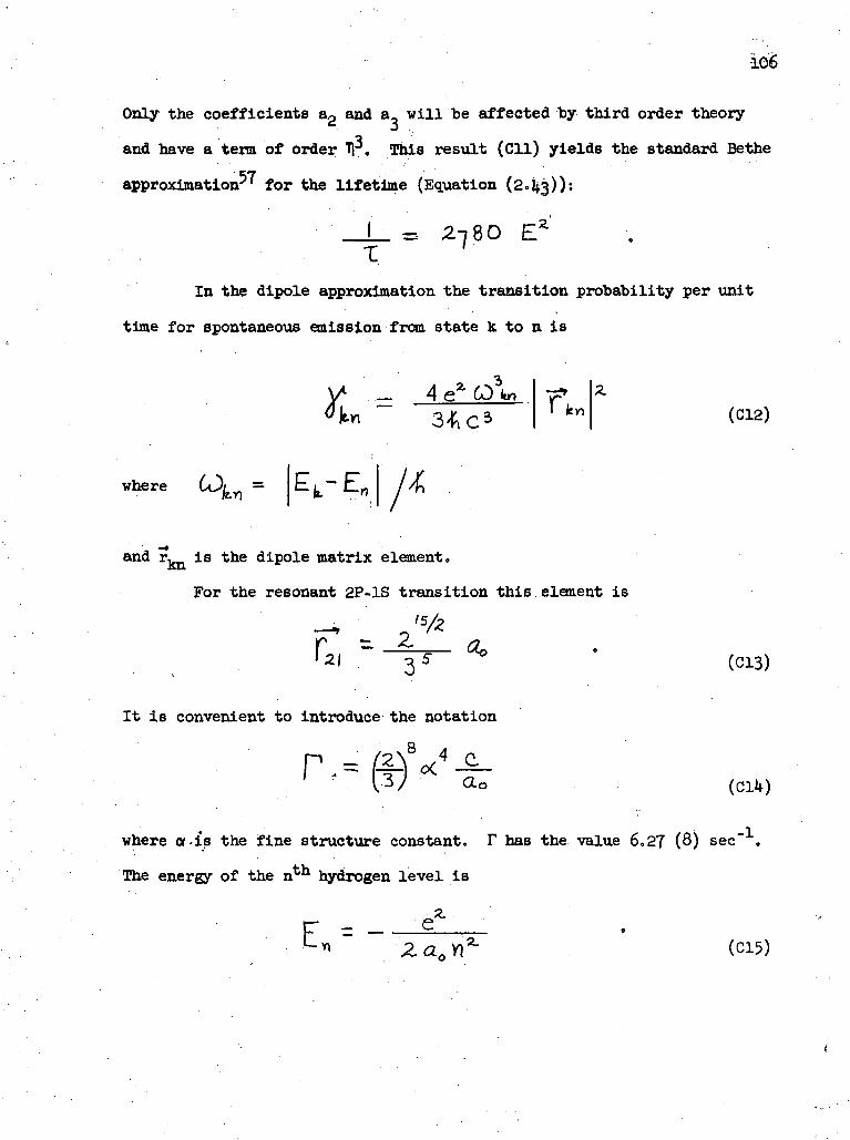
106
Only the coefficients a2 and a will be affected by third order theoryQ
and have a term of order Tp, This result (Oil) yields the standard Bethe
approximation" for the lifetime (Equation (2. 3)):
tIn the dipole approximation the transition probability per unit
time for spontaneous emission from state k to n is
._ A r,
where
and r,^ is the dipole matrix element <>
For the resonant 2P-1S transition this element is
-4 '5fcr,, ~ r- «*' 3
It is convenient to introduce the notation
8 A _P ~
(C12)
(ci3)
where a-is the fine structure constant. F has the value 6.2? (8) sec" .
The energy of the nth hydrogen level is
• *» Zann (C15)
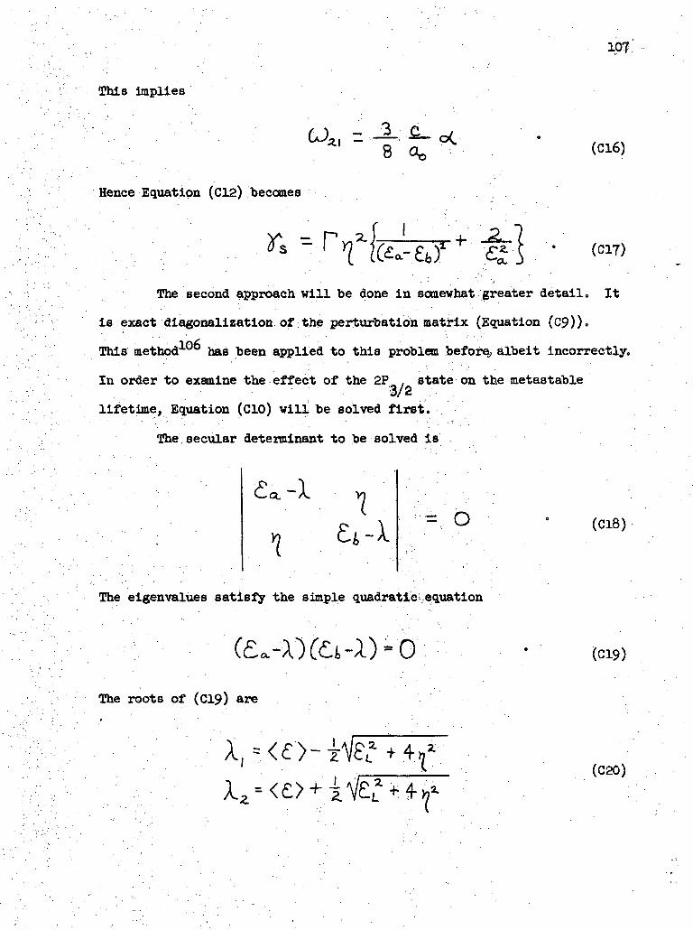
107
This Implies
= -3.8 (ci6)
Hence Equation (C12) becomes
; ' • (GIT)
The second approach will be done in somewhat greater detail. It
is exact diagonalization of the perturbation matrix (Equation (C9))«
This method106 has been applied to this problem before, albeit incorrectly.
In order to examine the effect of the 2P, , state on the metastable3/2
lifetime, Equation (CIO) will be solved first.
The secular determinant to be solved is
7= o (C18)
The eigenvalues satisfy the simple quadratic.equation
(019)
The roots of (C19) are
(C20)
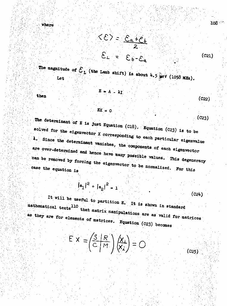
where
magnitude of
Let /
B « A - XI ;••'.•• C.C22)
' . : • - • • ' ' . ' ' . . . " • ' ' , ' ; . ' • . . • '
EX > 0 ' (C23). (C2
The determinant of £ is Juat Equation (Old). Equation (C23) is to be
solved for the eigenvector X corresponding to each particular eigenvalue
X. Since the determinant vanishes, the components of each eigenvector
are over-determined and hence have many possible values. This degeneracy
can be removed by forcing the eigenvector to be normalized. For thiscase the equation is
It will be useful to partition E. It is shown in standard
mathematical texts that matrix manipulations are as valid for matrices
as they are for elements of matrices. Equation (023) becomes
where S is a 1 x 1 matrix (really Just E, , )•'••.••'• ' • ' • • - • . . • - • ' . . ' • , . : ' • ' • • • ' : ••'"
R is a 1 x (n-l) row matrix V
C is an (n-l) x 1 coluan matrix v/
M is an (n-l) x (n-l) matrix
X-L is the first element of the X vector1 off (C23)
X. is the (n-l) element vector which was the rest of X.
Then Equation (C23) becomes
x RX, ;- 0 ; :V : : ; (C26)
This system of equations could be solved if the determinant did not
vanish. But from Equation (Cl8) it is seen that
: ;p^ RC > 0 '•••.-. (C27)
Since Equations (C26) are redundant/ pick the last of them to solve for
the ratio X /X o Then the equation is cast in the standard matrix form
of y = A x*. Also consider the solution of M using Cramer's rule. Then
X>L is easily seen to be proportional to the determinant of M°
For the 2 x 2 version of E, M is a single element. M is a
simple 2 x 2 matrix for the full treatment of this lifetime calculation
(Equation (C30)).
For the reduced matrix ( CIO)
. . . (028)- 1 1 . . ; • - • . . .
It is readily shown that these satisfy (C23). If Equation (02*0
is used to determine N, one finds that [to within an overall sign]
a -(G29)
^ =
These are shown in Figure C-2.
Consider now the 3 x 3 case represented by Equation (C9). In the
same way one obtains the secular determinant
1-0
O
-X•= o (030)
the eigenvalue equation
(C3D
and the eigenvectors
Ma,
(C32)
where
(C33)

There are two asymptotic regions of interest for each case; the
small 1) region and the high T) area. For the two state example the roots
become
.•;'"•' < A. - £*. -J_
2 = +1 4!2 • f S~and the coefficients approach
a, «s 11 (C35)
For large 1) the eigenvalues and eigenvectors "bee
" V (C36)
^ 2 a .•'•;: (C3T)
Figure C-3 shows the effect of an external field on a-j_ and a .
The three state example has the following zero field forms:
al
(C39)
Of course for slightly larger fields the two state approximation holds.
112
,-n3The third root is - !L , For large fields (11 » £a + £TJ) %ba secular
a • ' ' • ! •equation becomes approximately
- 3» aJl- ' (CUO)
Its roots are
A. = OonT5 vj ^ ~f3 * - t (GUI)
If the growth of the |a > state energy eigenvalue is followed as
the electric field increases, it becomes clear that the proper root is
the small one. Then the cubic equation can be truncated to a simple
linear one. It becomes
=0
Whence the small root is
= "2 C(, . ((A3)
Since a is independent of the electric field, it becomes negligible.
Hence the coefficients approach
They are displayed as a function of the field in Figure C-4, The
displacement of the "metastable" level appears in Figure C-3. Figure C-5
shows the uetastable lifetime as a function of applied field. The two
state value is the lover curve. The theoretical quadrupole lifetime
^8't.B added to this calctaation in that plot. Breit and Teller
" ' • ' • '• • "50 ' • • '•'• - ' • • • • /and Shapiro and Teller'* have assigned it a value of about 1/7 of a second,• i ' " • . _ "' ' . • ; . ' ' • • '
A more recent calculation 107 changes it to 1/3 second.
-f-
The third term in Equation (C 5) is due to a projected permanent- • ' • ' ' • • ' • • ' ' : ' . . " , • • • ' • - ; 3 i ' . •dipole moment in the atom. Fite et al. • have placed an upper limit on
this moment. They deduced a lover limit of &>k msec. This is the same
order as the earth field induced value of Section 5.3 « 2. It has been. • • :•• . . / • • • ". . '" -
neglected in the figures for this appendix.
Similarly Equation (C8) can be solved for the resonance states.
Then the following expansions occur:
For small;fields only bp and c_ are non-zero. ; For high fields the
asymptotes become '
(1/6)*
As a result of (d4-9) the lifetime of the resonant states increases to
2/r. The results of this calculation are shown in Figure C-6. The life-
times of the two 2P I substates that are not mixed remain at 1/F. These
are the "r" level in Figure C-l. Both C-l and C-2 are drawn using the
3 state expansion and equations (C32) and (C33).

APPENDIX D
CALCULATION j9P THE TWO WIRE FIELD
This is an appendix for those enamored with appendices. In order
to calculate the expected lifetime behavior of the metastable atoms as
they pass between the two wires which hang beneath the UV detector, it is
necessary to know the electric field generated by these wires. The wires
can be assumed to be cylinders of finite radius which are infinite in
extent along the z axis. The beam path is the y axis. The oven lies in
the negative y direction. The circular cross sections of the wires
determine the x axis. Consider this problem as a stack of x-y planes.
It then becomes a two-dimensional problem in any particular plane. It
can be shown that the equipotential surfaces in the plane are circles.
Further the electric field lines are arcs of circles that intersect the
wires. It is known that the equipotentials satisfy
V -A •+ y = (Dl)
where
,2
71.(D2)
The center and the radius of an equipotential circle are both functions
of the parameters s and m, M is the ratio of distances from the centers
and s is a function of the wire separation and wire radius.
115

116
In this experiment one wire is at potential V and the other one
is grounded. The potential at any point becomes
V(vn) = A U(von) -t- • (D3)
The midplane of symmetry (the y axis) is at potential V/2. To evaluate
the constant consider the potential difference between the midplane (ou>l)
and one wire (memo). Then
V2 In
(I*)
The separation between the wires (d) and the wire radius (ro) determine
m0. The relevant equations arei [
dm2-- 1 .'.(D5)
•w\ *• — I0 (P6)
Equations (D5) and (D6) are solved simultaneously to give
<Jo • b
The roots are approximately

117
.r-sLv- -£rc d
Note that they obey the general rule for points symmetrically placed
about the y axis ,
where the unpriced value refers to the positive y value and the primed
one to the negative value.
S may now be evaluated, D is the distance between the wire
centers. It is also the separation of the centers of the equipotentials
for m=m and m «fll . Thuso o . • - . - • ' • . : • . . ; . •
ri ^
Apply Equation (D9). Then Equation (DIO) becomes (D5). Square and
rearrange (D5) so that it beccmes ;
5 ='.(DU)
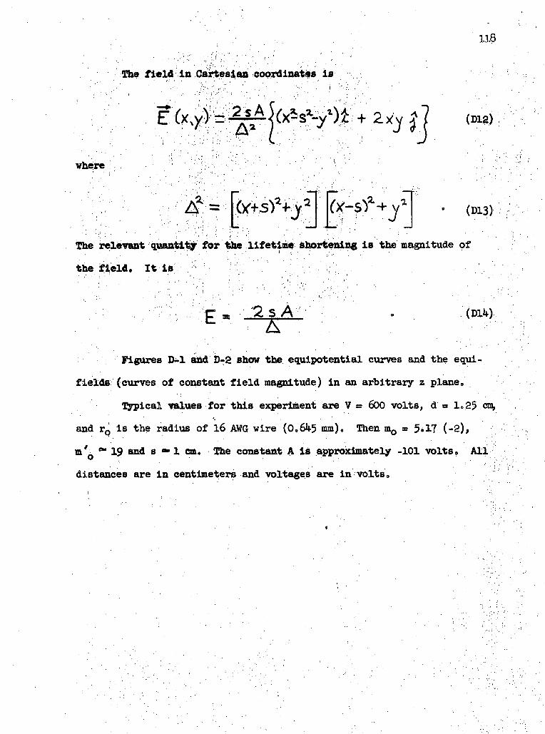
The field in Cartesian coordinates is
where
<*-sf+ ya, .':' ' »•/
118
(D12)
(D13)
The relevant quantity for the lifetime shortening is the magnitude of
the field. It is
2s A
Figures D-l and D-2 show the equipotential curves and the equi-
fields (curves of constant field magnitude) in an arbitrary z plane.
Typical values for this experiment are V * 600 volts, d «= 1.25 cm,
and rp is the radius of 16 AWG wire (0.645 mm). Then mo - 5*1? (-2),
m/6 °" 19 and s «*• 1 cm. The constant A is approximately -101 volts. All
distances are in centimeters and voltages are in volts.
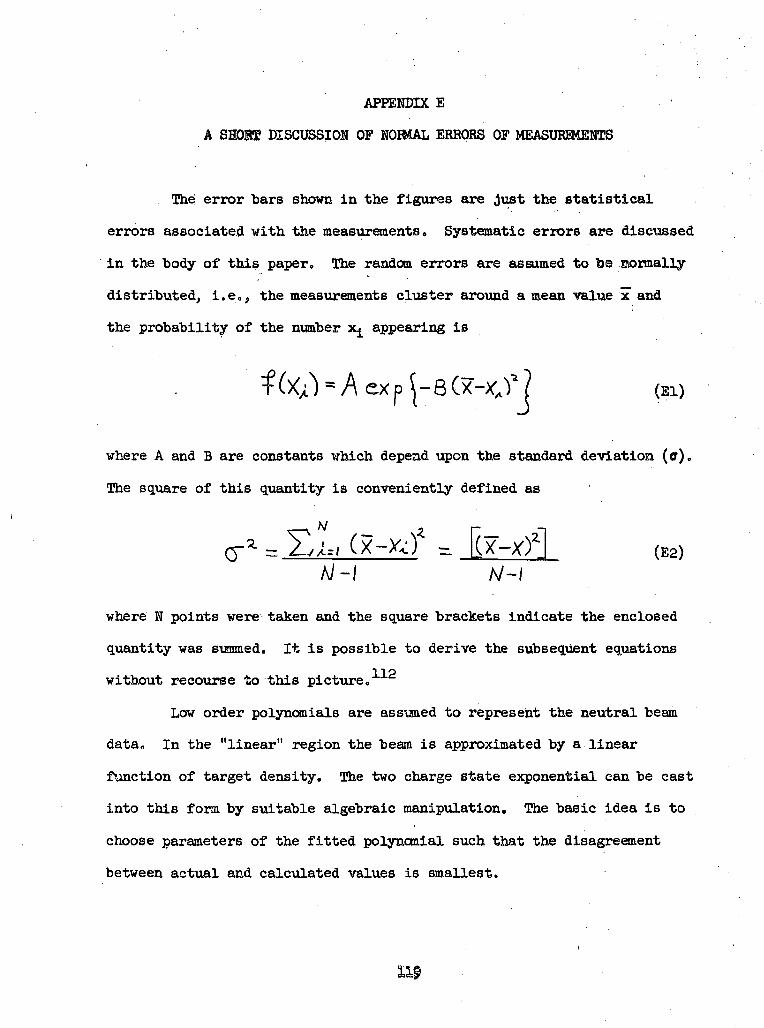
APPENDIX E '
A SHOBS DISCUSSION OF NOIMAL ERRORS OF MEASUREMENTS
The error bars shown in the figures are Just the statistical
errors associated with the measurements. Systematic errors are discussed
in the body of this paper. The random errors are assumed to be normally
distributed, i.e., the measurements cluster around a mean value jT and
the probability of the number x appearing is
i) = A ex - x- (EI)
where A and B are constants which depend upon the standard deviation (ff).
The square of this quantity is conveniently defined as
(E2)
A/-I A/-/
where N points were taken and the square brackets indicate the enclosed
quantity was summed. It is possible to derive the subsequent equations
UPwithout recourse to this picture.
Low order polynomials are assvmed to represent the neutral beam
data. In the "linear" region the beam is approximated by a linear
function of target density. The two charge state exponential can be cast
into this form by suitable algebraic manipulation. The basic idea is to
choose parameters of the fitted polynomial such that the disagreement
between actual and calculated values is smallest.

. •..•'".' . : ' ..'• !v. ' l£0
One minimizes the sums of the squares of these differences. This
is the least squares method of curve fitting. In addition some measure,
ments may be thought to be more accurate than others. Each datum can be
assigned a weight. This factor is related to title errors to be discussed
later. The suns are differentiated with respect to the several
parameters. This generates a system of equations relating the known data
points (xi) to the erroneous measured values (y ). For the above case
the target density is assumed to be exact whereas the measured neutral
fraction may contain errors. As long as the assumed functional form has
an additive constant, the sum of the differences must be zero.
For example, the linear form (y •» a + a.x) produces the
following simple set of equations:
[y] - aQH - ai[x] = 0
(E3)[xy] - a0[x] - a x2] *, 0
The sua of the squared differences becomes
a2 » [(iy- a - a,x)2]/(N-2) , (EU)O A
Two pieces of information are used to determine the coefficients. Hence
only N-2 data points are left to check the accuracy of these constants.
For a P parameter fit toe denominator would be N-P.
It is now assumed that all discrepancies between expected and
measured values are caused by errors in the coefficients. Also there are
P independent errors. It can be shown that the standard deviations
for a sum of independent measurements are related to the total standard
deviation through

121
(E5)
for Aibecomes
For a linear fit at a fixed x, thisi
(16)
where er is the error in aQ and
points Equation (E6) suns to
in the difference. For all N data
Equation (E5) oyerspecifles this problem of determining the coefficient
errors „ These can be found by applying the methods of Appendix C.
Alternatively one can note that Equation (E6) comes from a Taylor series
expansion. It expresses the difference as an error times the parametric
partial derivative of the measurements. Independence of the errors,
Equation (E5) and considerable manipulation leads to
CX'
|Mco
.~ ••• ~
M, MJLA.
(E8)
where JM | is the minor corresponding to the cofactor m.., i.e., the
determinant written without the i row and coltann. This is properly
normalized for the sun of the products of each cofactor and its minor is
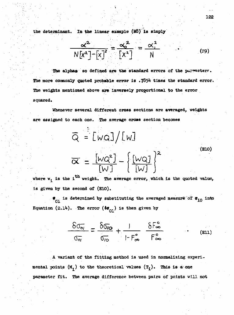
. = • ' • • ' ' ' ' -•'. .'."' : ':' ' ' . •• 122
the determinant. In the linear example (Ed) is simply
N
The alphas so defined are the standard errors of the
The more conmonly quoted probable error is .7854 times the standard error.
The weights mentioned above are inversely proportional to the error
squared*
Whenever several different cross sections are averaged, weights
are assigned to each one. The average cross section becomes• • ,
Q ='[K/Q]/[W]
or =[W]
[WQ] ][W] )
where wi Is the i weight. The average error, which is the quoted value,
is given by the second of (E10).
f.. is determined by substituting the averaged measure of <l 0 into
Equation (2.Ik). The error (**) is then given by
.(55 ( I-P.o pOoo I os
A variant of the fitting method is used in normalizing experi-
mental points (M.) to the theoretical values (T). This is a one
parameter fit. The average difference between pairs of points will not
123
vanish. If weights are assigned, the normalization constant satisfies
- [WTM]
" [W T T] (E12)
from the original equation
_ _dC
The error is the standard deviation divided by the square root of the
total weight. The £ of Figure 5-22 is one of the normalization constants
as calculated from. Equation (E12) . -
HELIOGRAPH*
1. W. Bleakney, Phys. Rev. 35; Il80 (1930).
2. P. T. Smith, Phys. Rev. 36, 1293 (1930).
3. J. T. Tate and P. T. Smith, Phys. Rev. 39; 2?0 (1932).
4. W. Bleakney, Phys. Rev. 40, 1*96 (1932).
5. A. Dalgarho and H. N. Yadav, Proc. Phys. Soc. A66, 173 (1953).
6. H, S. W. Massey and E. H. S. Burhop, Electronic and Ionic Impact
Phenomena, (Claredon Press, Oxford, 1952), Chapter 8.
7. W, R. Ott, W. E. Kauppila, and W. L. Fite, Phys. Rev. Letters 19,
1361 (1967).
8. J. B. Hasted, Advances in Electronics and Electronic Physics,
(Academic Press, New York, I960), Vol..XIII, pp. l-8l.
9- D, R. Bates and A. Dalgamo, Proc. Phys. Soc. A66, 972 (1953).
10. W. L. Fite, R. F. Stebfcings, D. G. Hummer, and R. T. Brackmann,
Phys. Rev. 119, 1939 (1960);
Phys. Rev. 124, 2051 (1961).
11. W. L. Fite, A. C. H. Smith, and R. F. StebMngs, Proc. Roy. Soc.
268, A527 (1962).
12. S. Dushman and J. M. Lafferty, Scientific Foundations of Vacuum
Technique, (John Wiley and Sons, New York, 1962), Table 10.1,
p. 696.
13. A, H. Futch and C. C. Damn, Nucl. Fusion 3, 124 (1963).
14. N. V. Fedorenko, V. A. Ankudinov, and R. N. II'in, Zh. T. F. 3J>
595 (1965), [Sov. Phys.- Tech. Phys. 10, 46l (1965) - English
translation].
124


125
15. C. C. Damm, J. H. Fotte, A. H. Futch, and R. F. Post., Phys. Rsv.
Letters 10, 323 (1963).
16. D. R. Sweetman, Nucl. Fusion, 1962 Suppl. Part \, d(9.
17. J. R. Hiskes, Nucl. Fusion 2, 38 (1962).
18. J. R. Hiskes, C. B. Tarter, and D. A. Moody, Phys. Rev. 133 . A424
(1964). • '
19. D. S. Bailey, J. R. Hiskes, and A. C. Riviere, Nucl. Fusion 5,
No. 1 (1965).
20. R. N. II'in, B. I. Kikiani, V. A. Oparin, E. S. Solov'ev, and
N. V. Federenko, Zh ETF 4J, 1235 (1964), [JETP 20, 835 (1965) -
English transl.].
21. R. N. Il'in, V. A. Oparin, E. S. Solov'ev, and N. V. Federenko, Zh
TF 36, 12 1 (1966), [Sov. Phys. - Tech. Phys. 11, 921 (196?) -
English transl.].
22. H. Bolen, G. Clausnitzer, and H. Wilsch, Zeits. Phys. 208, 159
(1968).
23. B. L. Donnally and W. Sawyer, Phys. Rev. Letters 15, 439 (1965).
24. B. L. Donnally, T. Clapp, W. Sawyer, and M. Schultz, Phys. Rev.
Letters 12, 502 (1964).
25. L. Madansky and G. Owen, Phys. Rev. Letters 2, 209 (1959).
26. L. Colli, F. Cristofori, G. Frigerio, and P. Sona, Phys. Letters 3;
62 (1962).
27. J. E. Bayfield, Phys. Rev. 1§2, 115 (1969).
28. J. E. Bayfield, Phys. Rev. Letters 20, 1223 (1968).
29. G. Ryding, A. B. Wittkower, and H. B. Gilbody, Proc. Phys. Soc.
(London) 89, 547 (1966).


126
30. D. R. Bates and G. Griffing, Proc. Phys. Soc. (Londcn) A66, 9ol
(1953).
31. D. Jaecks, B. Van Zyl, and R. Oeballe, Phys. Bcv. 137, A340 (1965).
32. W. L. Fite and H. T. Brackmann, Phys. Rev. 112, 1151 (1958).
33. G. H. Dunn, R. Geballe, and D. Pretzer, Phys. Rev, 128, 2 0
34. E. L. Cbupp, L. W. DotcMn, and D. J. Pegg, Phys. Rev. 175, 44
(1968).
35. M. Gryzinski, Phys. Rev. 11$, 374 (1959).
36. M. Gryzinski, Phys. Rev. 138, A305 (1965).
37. M. Gryzinski, Phys. Rev, 136, A322 (1965).
38. M. Gryzinski, Phys. Rev. 138, A336 (1965).
39. M. Gryzinski, Phys. Rev. Letters 14, 1059 (1965).
hO. J. D. Garcia, E. Gerjuoy, and J. E. Welker, Phys. Rev. 165, 66 ]
(1968).
41. P. A. Schnelzbach, W. Gruebler, V. Konig, and P. Marnier, Helv.
Phys. Acta la, 1<42 (1968).
42. A. S. Schlachter, P. J. Bjorkholm, D. H. Loyd, L. W. Anderson,
and W. Haeberli, Phys. Rev. 177, 184 (1969).
43. A Cesati, F. Cristofori, L. M. Colli, and P. Sona, Energia Nucleare
13,, 649 (1966).
44. I. A. Sellin, Phys. Rev. 136, A1245 (1964).
45. I. A. Sellin and L. Granoff, Phys. Letters 25A, 484 (1967).
46. G. Spiess, A. Valance, and P. Pradel, Abst. 7th Inty Conf. on
Phjysics of Electronic and Atoaic Collisions, Amsterdam, 1971 (North-
Holland Publ. Co., Amsterdam, 1971), pp. 823 - 824.
47. J. R. Oppenheimer, Phys. Rev. 31. 349 (1928).

127
WJ. Ho Co Brlatenan and H, A. Kramers, Proc,, Ac ad. Soc. (Amsterdam) 33;
973 (1939).
U9» D, Ro Bates sad A. Balgaras, Prec0 Pt s, Sec, (London) A6g, 919
(1952).
50. F. Ribe, Physo HQVO Jj, 1217 (I95l)o
51. j. DO Jackson and H. Scbiff, Pfeys. Rev. Sg, 359 (1953).
52« Jo R. Hiskes, Pbyao Rev, Af 3.T, 3 1 (195).
53o S. T. Butler and I. B, 8. Johnston, Pays. Letters g, lUl (1964)0
5^» So T« Butler, R« Mo May, and I» B0 8. Johnston, Flays « Letters
55<> 3. To Bulter and I. B. 8. Johnstoa, Hud. Fusion jt, 196
Fusion"
57" Ho Ao Bethe and E, H. Salpeter, Encyclopedia of Physics (Springer-
Verlag, Berlin, 1957)., Vol. X3EXV, p. 370,
58, S. Breit and §o Teller, Astrophys. J0 y 215 ( 19 *0) .
59» Jo Shapiro and 9, Breit, Phys. Rev. 113, 179 (1959).
60o W. L. uiese, Mo W« ifiithj, and B« M. Glennon, Atoaic Transition
ProibabllitlBS, NBS Ctrc, k (U. S. Govt. Printing Office, Washington,
1966), Vol. lo
6l. Obtained from Radiation Dynamics, Inc0, Westbury Industrial Park,
Westbury, Lo&g island.
62o The mixture is RCA No. 330=118 available from the Harriflon, New
Jersey plant of RCA.
63. R» To Brachmamv W. L. Fite, and Ko £. Hagen, Rev, (lei. $nst»
125 (195B).

128
6k. P, H. Metzger and G. R. Cook, J. Quant, Spectrosc. P.adiat.
Transfer 4, 107 (1964).
65. Obtains* frcm larshaw Chemical Co., 19lf5 E. 97tli Street, Cleveland
6, Ohio.
66. W. M. Preston, Phys. Rev. 57, 88? (I9lt0)0
67. Y. Tanalca, E. C. Y. Inn, and K. Watanabe, J. Ctveau Phys, 21, 1651
(1953).
68. W. E. Kauppila, W. R. Ott, and W. L. Fite, Rev. Sci. last. 38,
811 (1967).
65. W. R. Ott, "Polarization of Lyman Alpha Radiation Baitted in
Electron-Hydrogen Atom Collisions and Emitted "by Metastable H(28)
Atoms in Weak Electric Fields", Ph.B. Thesis, ttai-Wrtltty of
Pittsburgh, 1968 (unpublished).
70. See for example; H. B. Callen, Thermodynamics (John Wiley and Sons,
New York, 1963), Chapt. 17.
71. E. G. Schneider, Phy». Rev. 3 1 (1936).
72. K. Watanabe, E. Inn, and M. Zelikoff, J. Chat. Bay*. 20, 19 9
(1952).
73« R. W. Ditchburn, J. E. S. Bradley, C0 G. Cannon, and G. Munday,
Rocket Exploration of the Upper Atmosphere (Pergamon Press, London,
195 ), R. L. F. Joyd and M. J. Seaton, editors, pp. 32? - 33 v
7 . P. Lee, J. Opt. Soc. Amer. \ 703 (1955).
75. K. Watanabe, Advances in Geophysics (Academic Press, New York,
1958), H. E. Landsberg and J. Van Mieghem, ed., Vol. 5, pp. 151
- 221.

• • : • • ' 1 2 9
76. See for example: A. G. P»ch»lczyk, Radio Astrophysics (W. E*
Freeman, San Fraacisco, 1970), Chapt. 5.
77. D. Pretzer, B. Vaa Zyl, amd R. Qeballe, Fhy». Pe-». Letters 10, ;jliO
(1963).
78. L. Harris and J. K. Beasley, J, Opt. Soc. Aaer. b2j 134 (I25?)«
79. V. V. Gritsyna, T. S. Kijan, A. G. Koval', and Ja« M» Fogel1,
Pays. Letters 27A, 292 (1968).
80. A. A. Sterk, C. L. Marks, and W. P. Saylor, Phys. Rev. Letters 17,
1037 (1966).
81. R. Kieman, T. M. Donahue, and K. Lulla, Bull. Am. Phys. Soc. 12,
llU (1967); R. A. Nieman and T. M. Donahue, Bull. Am. Phys. Soc.
13, 66 (1968);
R. Nieman, K. Lulla and T. M, Donahue, Abst. 5th Int. Conf. on
Phys. Electronic and Atomic Collisions, Leningrad, 1967 (Nauka,
Leningrad, 1967), pp. 18-19.
82. A. V. Viriogradov, L. P. Presnyakov, and V. P. Shevel'ko, Zh ETP
Pis. Red. 8, W9 (1968), [JETP Letters §, 275 (1968) - English
transl.]
83. J. A. Bearden and A. F. Burr, Rev. Mod. Phys. 39, 125 (1967).
84. E. Gerjuoy, Phys. Rev. 11*8, '5_4 (1966).
85. S. K. Allison, Rev. Mod. Pfcfrtt. 32, 1137 (1958).
86. G. W. McClure, Phys. Rev. 130, 1852 (1963).
87. B. Van Zyl, D. Jaecks, D. Pretzer, and R. Geballe, Phys. Rev. 156,
29 (1967).
88. J. D. Jackson, Classical Electrodynamics (John Wiley and Sons,
York, 1962), p. 380.
130
89. E. M. Purcell, Astrophys. J. 116, 57 (1952).
90. M. J. Seaton, Proc. Phys. Soc. (London) A68, lt-57 (I95!l).
91. L. R. Wilcox and W. E. Lamb, Jr., Phys. Rev. 119, 1915 (x oO).
92. J, I. Gersten, J. Chem. Phys. 51, 63? (1969).
93. M. Bloom, I. Oppenheim, M. Lipsicas, C. G, Wade, and C. F.
Yarnell, J. Cheai. Phys. 1*3, 1036 (1965)-
9 . A. L. McClellan, Tables of Experimental Dipole Moments (W, H.
Freeman, San Francisco, 1963).
95« V. Dose, V. Meyer, and M. Salzmann, J. Phys. B. (Atom. Molec,
Phys.) 2, 1357 (1969).
96. H. B. Gilbody, R. Browning, R. M. Reynolds, and G. I. Riddell,
Abet. 7th Int. Conf. on Phys. Electronic and Atomic Collisions,
Amsterdam, 1971 (North-Holland Publ. Co., Amsterdam, 1971),
pp. 1080 - 1082.
97. G. Spiess, A. Valance, and P. Pradel, Abst. 7th Int. Conf. on
Phys. Electron. Atom. Coll., Amsterdam, 1971 (North-Holland,
Amsterdam, 1971), pp. 1083 - 1084.
98. D. R. Bates and J. C. G. Walker, Planet. Space. Sci. l4, 1367
(1966).
99« G. Herzberg, Atonic Spectra and Atomic Structure (Dover Publica-
tions, New York, 19MO, Chapter 2.
100. J. A. Phillips and J. L. Tuck, Rev. Sci. Inst. 27, 97 (1956).
101. See for example; R. K. Eisenschitz, Matrix Algebra for
Physicists (Plenxsa Press, New York, 1966).
102. E. U. Condon and G. H. Shortley, The Theory of Atomic Spectra
(Cambridge Uhiv. Press, Cambridge, 1963).

131
103. L. Green, P. Rush, and C. Chandler, Astropby. J. Su pl. Ser. 37
(1957).
104. J. D. Jackson, Classical Electrodynamics (John Wiley, New York, 1962),
PP. 502, 558.
105. H. A. Bethe and E. E, Salpeter, Quantum Mechanics of One- an* Tw.o
Electron Atoms (Springer-Verlag, Berlin, 1957)*
106. G. Luders, Z. Naturforsch. 5_a, 608 (1950).
107. V« Zhukovskii, M. Kolesnikova, A. Sokolov, and I. Kaerrmann,
Optika i Spekt. 28, 622 (1969), [Opt. and Spectroc. 28, 337 (1970)
- English transl.].
108. W. E. Lamb and R. C. Rutherford, Phys, Rev. 79, 5 9 (1950).
109. See for example; L. I. Schiff, Quantum Mechanics (McGraw-Hill Book
Co., New York, 1955), Chapter 7.
110. See for example; S. Perlis, Theory of Matrices (Addison-Wesley
Press, Cambridge, Mass., 1952).
111. See for example; E. M. Pugh and E. W. Pugh, Principles of
Electricity and Magnetism (Addison-Wesley Publ. Co., Reading,
Mass., I960), pp. 116 - 122.
112. 3. R. Cohen and J. W, M. DuMond, Encyclopedia, of Physics
(Springer-Yerlag, Berlin,. 1957), Vol. XXXV, .pp.-. 1 -,87.
113. See for example; J, Topping, Errors of Observation and Their
Treatment (Reinhold Publishing Co., New York, 1958), Chapters 2 and
3. ' . • •
Ilv. Handbook cf Chemistry and Physics., k-kth Edition, Cheia. Rubber
• .. . Publishing Co., 1961, pp.' 3513-351 . •''•'• •

132
115. Handbook of Chemistry and Physics, l»4th Edition, Chem. Rubber
Publishing Co., 1961, pp. 2 16-2417.
116. E. J. Stone (private communication).
117. C. E. Moore, NBS Circ. k6j, U. S. Govt. Printing Office, Vol. I
(1950), II (1952), III (1958).
LIST OF TABLES
Table 1.1. A abort guide to cross section*.
Table 2*1. Maximum Gryzinski cross sections.
Table 3*1. Standard points for the thermocouple calibration.
Table 3.2. Molecular oxygen UV windows.
Table kti. Alkali density constants.
Table 5,1. Summary of p + K Results.
Table 5.2. Svmmary of p + Na Results.
Table 5.3. Summary of Hg+ Results.
Table 5.4. Alkali binding energies.
Table 5.5. Best values for the background H2 values of n and n
as deduced from measured 6 values.
Table 5.6. Purcell alkali quenching cross sections.
Table 5.7. Purcell-Seaton proton syarm quenching transition rates.
Table 5.8. Gersten molecular quenching cross sections*
Table B.I. Condon and Shortley corrections,,
Table B.2. Hydrogen transition probabilities and lifetimes.
133

TABLE 1.1.
A Short Guide to Cross Section*
Alkali EC MX F*«
Lithiua 21
Sodim 21 21
PotMsiua 21,1*1 1*5 21, la
Rubiditm 45
Cesim 21,1*2, W Sfc,1*3, 5, 6 21,1*2

135
TABLE 2.1.
Maximum Gryzinski Cross Sections
Alkali
Lithium
Sodium
Potassium
Rubidium
Cesium
raLAJ
1.52
1.86
2.27
2.48
2.65
SnaxLA J
(Eq.n. 2.27)
55.2
68.2
98.2
110.2
126.8
EplkeVJ
(* 0.1)
1.4
1.4
1.0
0.8
0.6
( J.' ,00)
20.6
24.3
45.7
53.6
74.4

TABLE 3.1.
Standard Points for the Thermocouple Calibration
Standard Point T['C]
LN2 -195.80
co2 - 78.51Ice 0.00
Steam 100.0
Tin 231.85
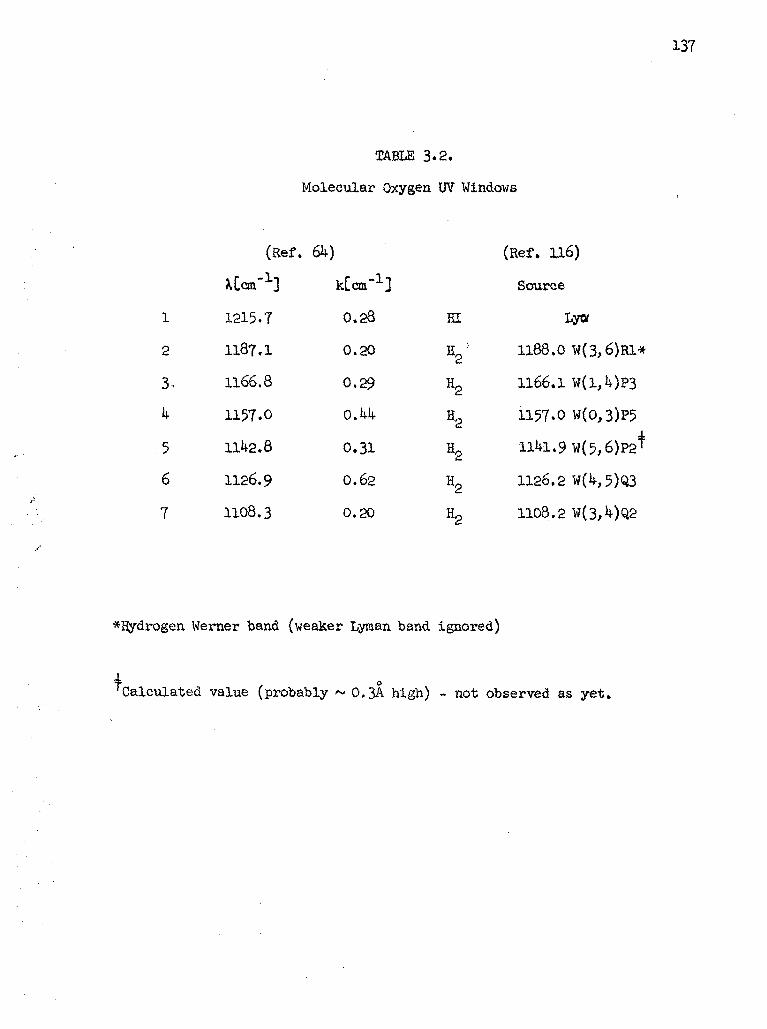
137
TABLE 3.2.
Molecular Oxygen UV Windows
(Ref. 6k) (Ref. 116)
1
2
3,
k
5
6
7
tf -l-I
1215.7
1187.1
1166.8
1157.0
1142.8
1126.9
1108.3
kCcm-1]
0.28
0.20
0.29
O.Mv
0.31
0.62
0.20
HI
V
H,
H,
H2
H2
H0
Source
Lytt
1188.0 W(3,
1166.1 W(l,
1157.0 w(o,
1114-1.9 w(5,
1126.2 ¥(i)-,
1108.2 ¥(3,
6)R1*
10P3
3)P5
f
5)Q3
U)Q2
*Hydrogen Werner band (weaker Lyman band ignored)
'Calculated value (probably ~ 0.3A high) - not observed as yet.
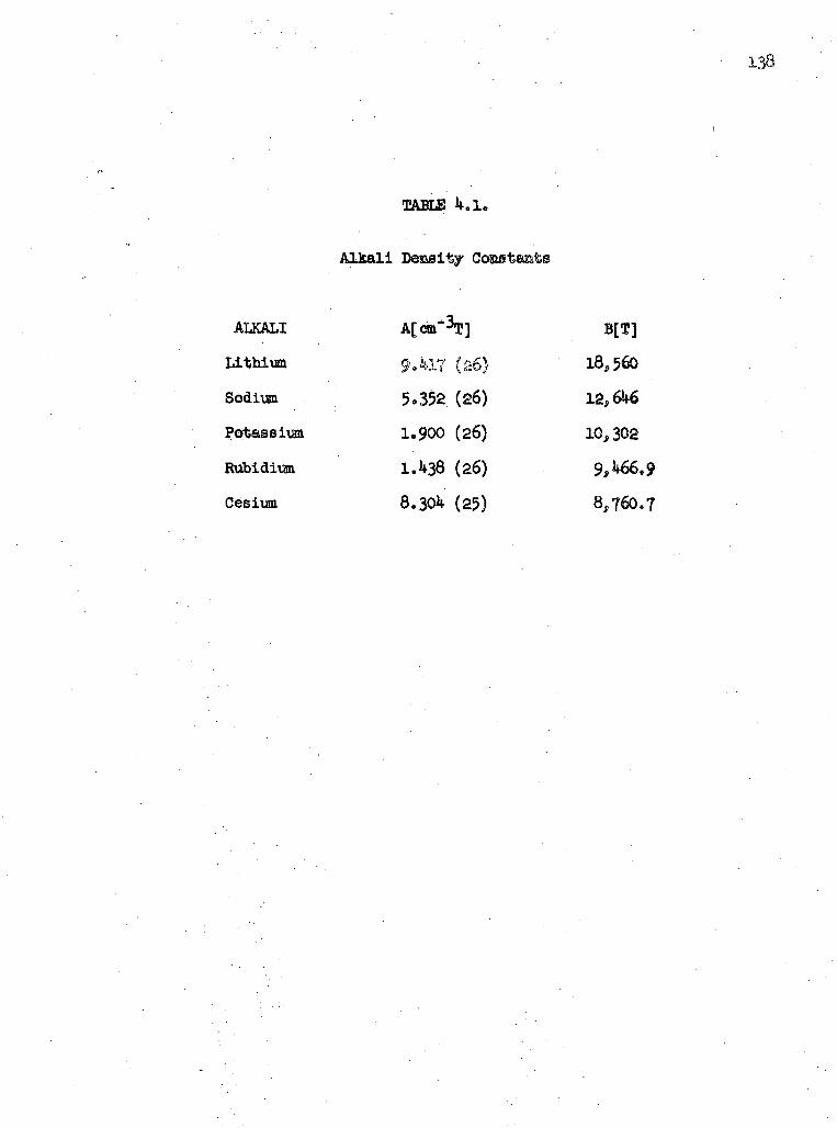
TABU! 4,1.
Alkali Density Cojaetaats
138
ALKALI
Lithium
Sodium
Potassium
Rubidium
Cesium
A[cm"3T]
9.M7 (26)
5o352 (26)
1.900 (26)
1.1*38 (26)
8.304 (25)
B[T]
18,560
12,646
10, 302
9,466,9
8,760.7
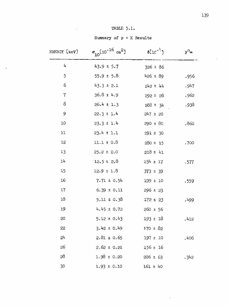
139
TABLE 5.1.
Summary of p + K Results
ENERGY [keV]
4
5
6
7
8
9
10
11
12
13
14
15
16
17
18
19
20
22
24
26
28
30
In 90 L10~ cm ]
43-9 ± 5.7
55-9 ± 5.8
43.3 ± 2.1
36.8 ± 4.9
26.4 ± 1.3
22.3 ± 1.4
23.3 ± 1.4
23.4 ± 1.1
ll.l ± 0.8
25-2 ± 2.0
12.5 ± 2.8
12.9 ± 1.8
7.71 ± 0.54
6.39 ± 0.11
5.11 ± 0.38
4.45 ± 0.72
5.12 ± 0.43
3.42 ± 0.49
2.81 ± 0.65
2.62 ± 0.21
1.98 ± 0.20
1.93 ± o.io
6[ic:]
326 ± 86
426 ± 89
242 ± 44
292 ± 28
288 ± 34
247 ± 20
290 ± 80
291 ± 30
280 ± 15
218 ± 4i
234 ± 17
373 ± 39
199 ± 10
296 ± 23
172 ± 23
260 ± 56
193 ± 18
1.70 ± 82
197 ± 10
156 ± 16
206 ± 63
161 ± 4o
F°<°
.956
.9*7
.962
.938
.860
.700
.577
.559
.499
.412
.4o6
.3 2
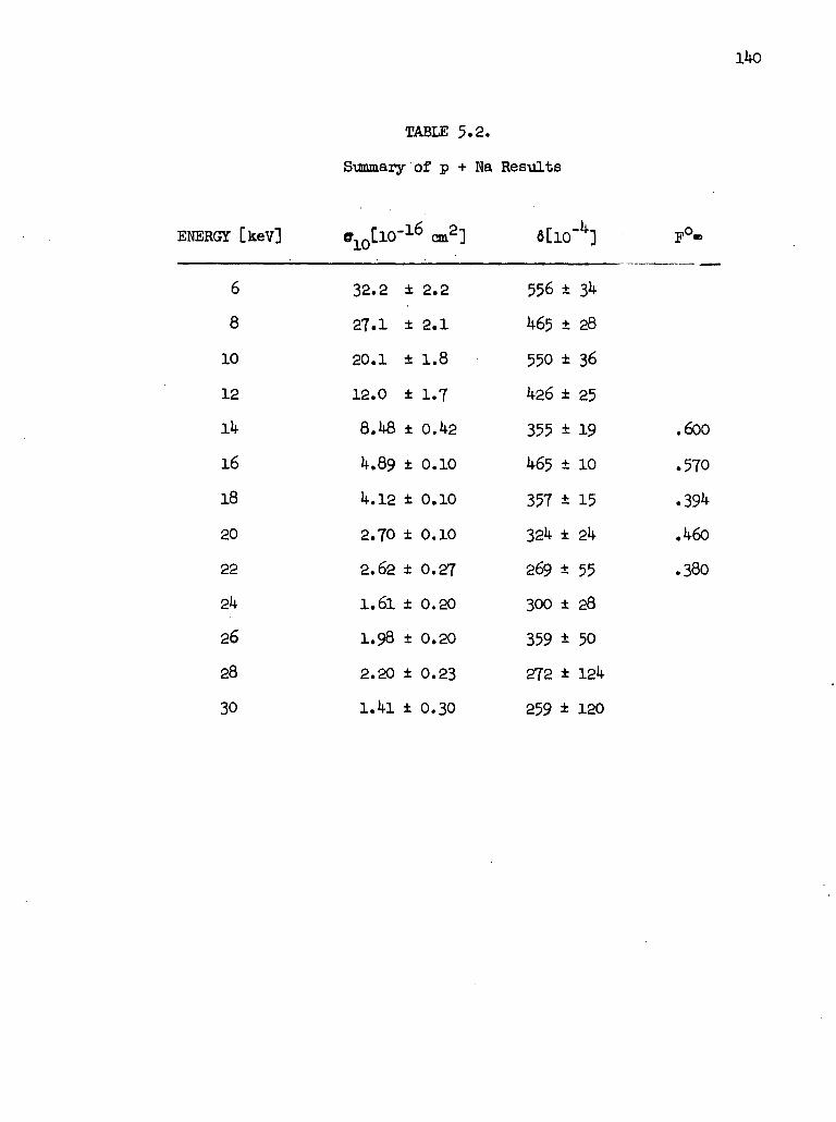
l4o
ENERGY [keV]
TABLE 5.2.
Summary of p + Na Results
6
8
10
12
14
16
18
20
22
24
26
28
30
32.2 ± 2.2
27.1 ± 2.1
20.1 ± 1.8
12.0 ± 1.7
8.48 ± 0.42
4.89 ± o.io
4.12 ± 0.10
2.70 ± o.io
2.62 ± 0.27
1.61 ± 0.20
1.98 ± 0.20
2.20 ± 0.23
1.41 ± 0.30
556 ± 34
465 ± 28
550 ± 36
426 ± 25
355 ± 19
465 ± 10
357 * 15
324 ± 24
269 ± 55
300 ± 28
359 ± 50
272 ± 124
259 ± 120
.600
.570
.394
.460
.380
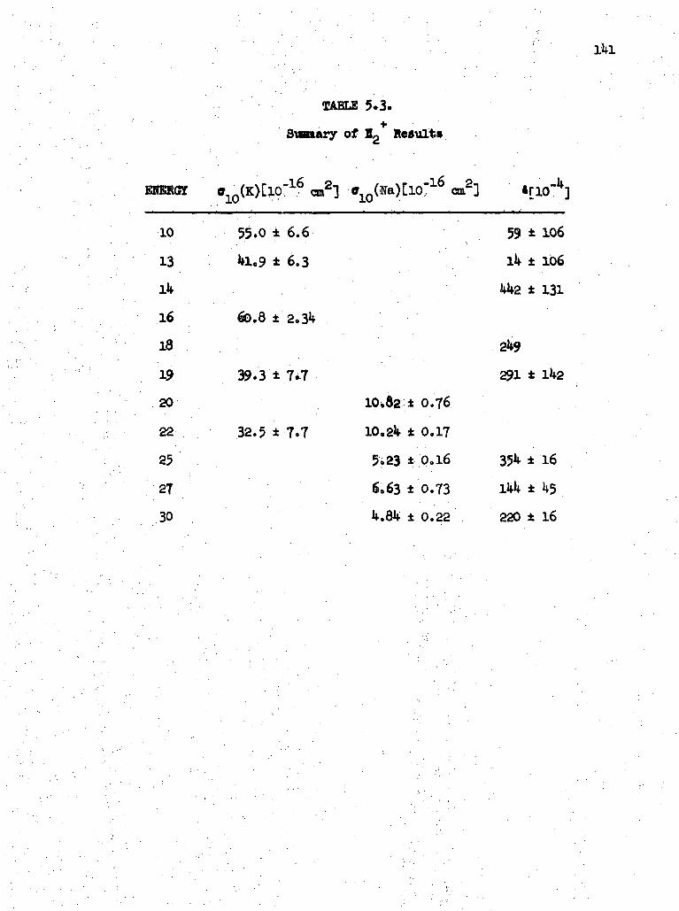
TABLE 5.3.+
Svnaary of I Result*
EMSRta 010(K)Cl9"16 cm2! »10(Na)[lo;16 cm2]
10
13
Ik
16
18
19
20
22
25
27
30
55.0 ± 6.6 59 ± 106
41.9 ±6.3 14 ± 166
442 ± 131
60.8 ±2.34
249
39.3 ±7.7 291 ± 142
10b$2 ± 0.76
32.5 ±7.7 10.24 ± 0.17
5.23 ±0.l6 354 ± 16
6.63 ± 0.73 144 ± 45
4.84 ± 0.22 220 ± 16

TABLE 5.4.
Alkali Binding Energies
ELEMENT
Valence Electron [117] Inner Shell [83]Binding Binding
Configuration Energy Configuration Huergy
3-
11
19
37
55
LithiVBBL
Sodium
Potassium
Rubidium
Cesium
28^ 5.390
3S, 5.138
4S% 4.339
5S% 4.176
6s^ 3.893
(is)2
(2p)6
(3s)2
<3p)6
p
. :'a|-;6r
(4p)
(5s>2
• -'^M^- • .
54.75
31.1
33.9
17.8
29.3
, 14.8
14.0
22.7
, 13.1f :
* 0.02
* 0.4
4 0.4
i 0.4
A 0.4
±0.4
±0.3
± 0,5
± Oo5
* 0.5

TABLE 5.5.
Best Values for the Background Ig Yaluee or
it and n as Deduced from Measured 6 Values
PROBE '-•"'..., •,..•' TARCB3T
K Ha K + Na
6.80 ±6.15(13) n.O ±8.5 (13) 7.76 ± 6.88 (13)
[a] 2. 3 2.20(12) 3.8 ± 3.<
H [u] 8.50 ±71.10(13)
[n] 3.0 ± 25.1*0(12)
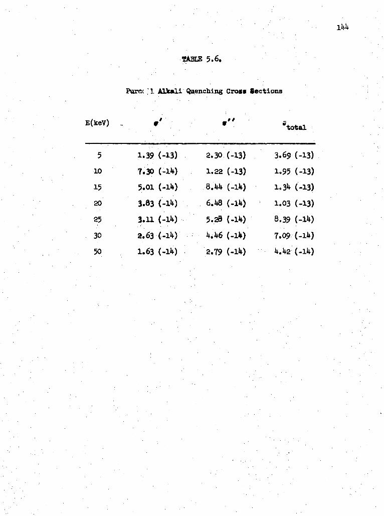
144
TABLE 5.6.
Purcc ;.l Alkali Quenching Crow Sections
E(keV) ., 9' •" "total
5
10
15
20
25
30
50
1.39 (-13)
7.30 (-14)
5.01 (-HO
3.83 <-U)
3.11 (-U)
2.63 (-14)
1.63 (-14)
2.30 (-13)
1.22 (-13)
8.44 (-14)
6.48 (-14)
5o28 (-14)
4.46 (-14)
2.79 (-14)
3.69 (-13)
1.95 (-13)
1.34 (-13)
1.03 (-13)
8.39 (-14)
7.09 (-14)
4.42 (-14)
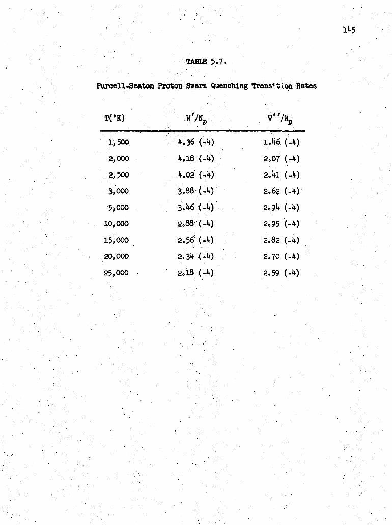
TABLE 5-7.
Purcell-Seaton Proton Swarm Quenching Transition Rates
K'K). wX x'V*n
1,500
2,000
2,500
3,000
5,000
10,000
15,000
20,000
25,000
M6 (-10
Wi8 (-10fc.02 (-10
3.88 (-U)
3.f* {-10
2.88 (-4)
2,56 (JO
2,31* (-10
2,18 (-If)
1,1*6 (-10
2,07 (-10
2.1*1 (-1*)
2.62 (-4)
2.91* (-M
2,95 (-^)
2,82 (-1*)
2.70 (-1*)
2,59 (-V
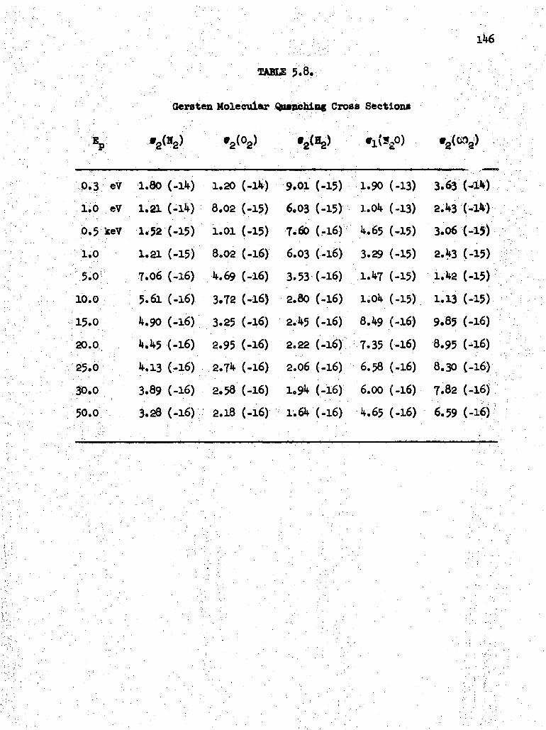
TAHE 5.8.
Qersten Molecular Quaachinc Cross Sections
: p 22 2 2
0,3 eV
1.0 eV
0.5 keV
uo';.5.or. .10.0
15.0
20.0:
25.6
30.0
50.0.
1.80 (-ifc)
1.21 (-110
1.52 (-15)
1.21 (-15)
7.06 (-16)
5.61 (-16)
1 .90 (-16)
U.1^5 (-16)
1M3 (-16)
3.89 (-16)
3.28 (-16)
1.20 (-HO
8.02 (-15)
1.01 (-15)
8.02 (-16)
if. 69 (-16)
3.72 (-16)
3.25 (-16)
2.95 (-16)
2.71* (-16)
2.58 (-16)
2.18 (-16)
9.01 (-15)
6*03 (-15)
7.60 (rl6)
6.03 (-16)
3.53 (-16)
2.80 (-16)
2.A5 (-16)
2.22 (-16)
2.06 (-16)
1.91* (-16)
1.6U (-16)
1.90 (-13)
l.Ok (-13)
V.65 (-15)
3.29 (-15)
l.Vf (-15)
1.CA (-15)
8.lf9 (-16)
7.35 (-16)
6.58 (-16)
6.00 (-16)
4.65 (-16)
3.63 t-i*)2.1f3 (^)
3.06 (-15)
2.U3 (-15)
1. 2 (-15)
1.13 (-15)
9.85 (-16)
8.95 (-16)
8.30 (-16)
7.82 (-16)
6.59 (-16)
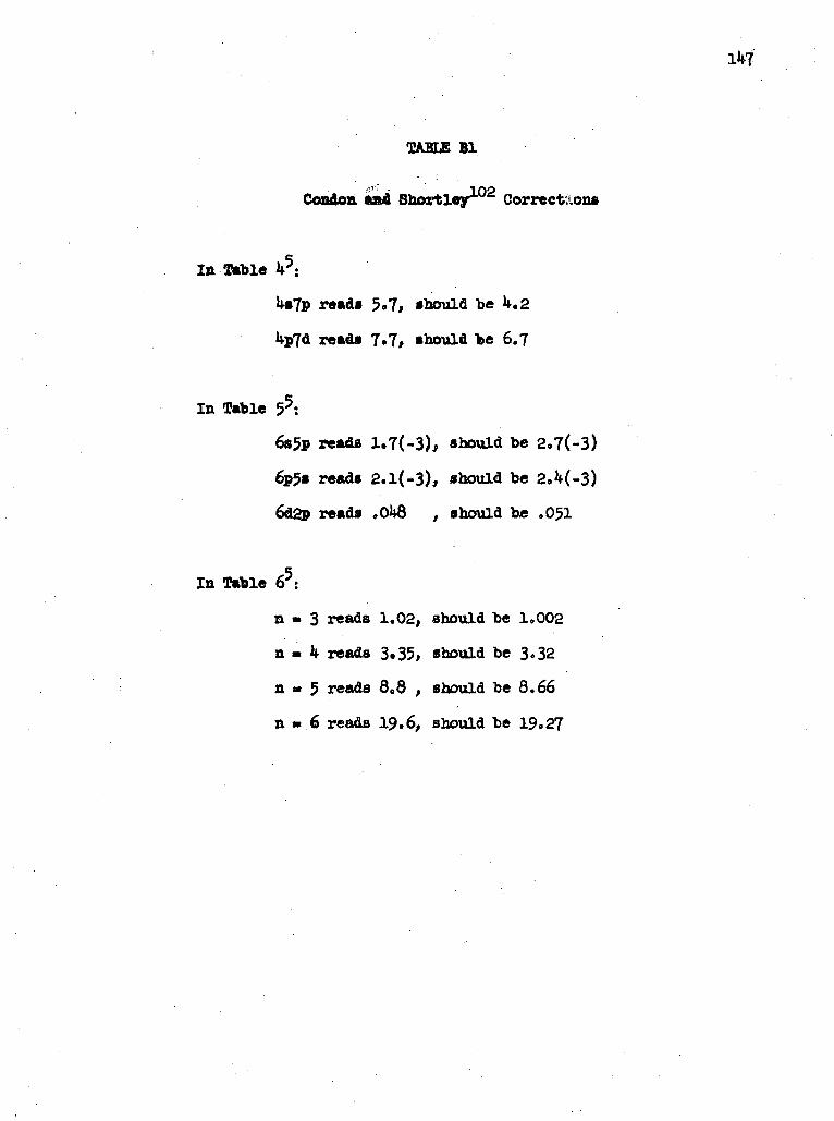
Ifcf
TABUS Bl
Condon auad Shortlejr02 Corrections
In Table 45:
l*»7p read* 5.7, should be ^.2
read* ?o?/ «houLd Tec 6.7
In Table 55:
6s5P reads 1.7(-3), should be 2.7(-3)
6p5« reads 2.l(-3), should be 2» (-3)
6d2p reads .01)8 , should be .051
In Table 65:
n • 3 reads 1.02, should be 1.002
n m k reads 3. 35, should be 3.32
n » 5 reads 8.8 , should be 8.66
n » 6 reads 19,6, should be 19.27

148
Transition Probabilities and
a
2
3
4
5
6
7
8
9
10
11
12
I
4.
9.
3.
1.
5.
2.
1.
8.
5.
3.
2.
•
WBSl
699
985
019
156
191
617
436
450
236
391
277
60t.
(8)
(7)
(7)
(7)
(6)
(6)
(6)
(5)
(5)
(5)
(5)
4,
9.
3.
694
975
016
1.155
5.189
2.612
1.
8.
5.
3.
436
462
214
380
2.284
102f .08
(8) 2.1
(7) 10.2
(7) 33.5
(7) 88
(6) 196
(6)
(6)
(5)
(5)
(5)
(5)
2.
10.
33.
86.
r *M*
130 l.i
02 3.5
15 8.7
61 IB
192.7 34
382.
696.
1182
1918
2959
4378
9 .055*8
2 .088ns
.14*8
.20|*s
.29UB
.3911.
T/014
3.0
23
96
294
731
1.6)48
3*1^8
5.5»*s
9.^*8
15 V-B
23 PS
T 105
8.5
53
192
525
1193
2.%kB
4.4»8
T.^is
12 MS
18 MS
27 IAS
Lifetimes «r« fiven in nsee unless otherwise noted.
Transition probabilities are given in sec" .
TW means this work.

FIGURE CAPTIONS
Figure 2-1. Bates and Dalgarno cross section for charge exchange
"between protons and potassium.
Figure 2-2. Bates and Dalgarno cross section for charge exchange
"between protons and sodium.
Figure 2-3. May calculation of the angular momentum state of atoui"
hydrogen produced during p + H collisions.
Figure 2-4. Contributions to -.Q Q-, for p + K from various atonic
hydrogen levels.
Figure 2-5. Gryzinski calculation of 10Qoi for "various alkali targets.
Figure 2-6. Same but for 1C)Q01(2S) assuming N(2S)/N(2P) = 1/3.
Figure 2-7. Predicted ratio of MX:TX assuming statistical weight
population of state.s as a function of proton energy.
Figure 2-8. Metastable populations of the n = 2 states.
Figure 2-9« Same but assuming only S state captures.
Figure 2-10. Relative 23 population as a function of beam energy.
Figure 3-1. Schematic view of apparatus.
Figure 3-2. . The neutral beam detector. ,
Figure 3-3« Schematic view of detection chamber and counter electronics.
Figure 3-4. Schematic view of electron gun.
Figure 3-5. Molecular oxygen window near 1216A.
Figure 3-6. Relative transmission of oxygen filter for Lyman alpha for
x = 2 atm-cm.
Figure 3-7. Integrated transmission of the oxygen filter as a function
of the viewing angle 6Q.
149
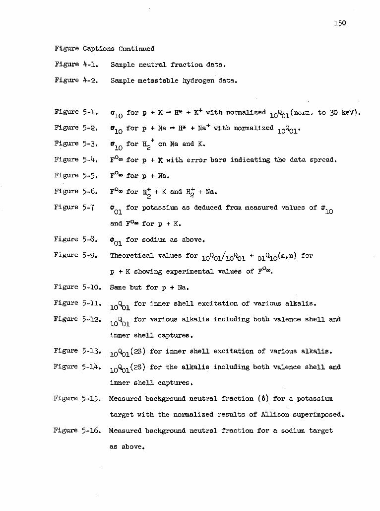
150
Figure Captions Continued
Figure 4-1. Sample neutral fraction data.
Figure 4-2. Sample metastable hydrogen data.
Figure 5-1. a1Q for p + K =• H* + K+ with normalized ( {nou r., to 30 keV),
Figure 5-2. OIQ for p + Na -» H* + Na+ with normalized 10%l*
Figure 5-3. o for E^ on Na and K.
Figure 5-4. F°® for p + K with error bars indicating the data spread.
Figure 5-5. F°» for p + Na.
Figure 5-6. F°<» for H+ + K and H£ + Na.
Figure 5-7 ffm for potassium as deduced from measured values of @ n
and F°*» for p + K.
Figure 5-8. eu, for sodium as above.
Figure 5-9. Theoretical values for lo Ol/loS}! + oAo(m>n) for
p + K showing experimental values of Fo°°.
Figure 5-10. Same but for p + Na.
Figure 5-11. , 0., for inner shell excitation of various alkalis.
Figure 5-12. ,nQm for various alkalis including both valence shell and
inner shell captures.
Figure 5-13. ,OQQ, (2S) for inner shell excitation of various alkalis.
Figure 5-14. -loQoi 23) for the alkalis including both valence shell and
inner shell captures.
Figure 5-15- Measured background neutral fraction (8) for a potassium
target with the normalized results of Allison superimposed.
Figure 5-l6. Measured background neutral fraction for a sodium target
as above.

151
Figure Captions Continued
Figure 5-17* typical low density results for 16 keV protons on sodium -
slight curvature of the "metastable" signal.
Figure 5-l8« Same as above but for 20 keV protons • pronounced curvature
of "metastable" signal.
Figure 5-19 • in^m ^or Pr°t°ns on excited sodium and potassium assuming
only valence electron contribution.
Figure 5-20. e (23) values of Sellin and Granoff for p + Cs, p + Rb
and p + K with normalized Gryzinski calculation ,0Q01(2S) .
Figure 5-21. CT10(2S) values of Donnally (Ref."2 ) for p + Cs with
normalized -_Qn (2S) calculation.
Figure 5-22. C,Q for p + Cs [Schlachter] and normalized inQm •
Figure A-l. Beam charge states and the associated cross sections.
Figure C-l. Splitting of the first excited state of hydrogen as a
function of external field.
Figure C-2. Behavior of 2S state as a function of applied field.
Figure C-3. Mixing coefficients of the two level approximation.
Figure C-k. Mixing coefficients of the three state approximation.
Figure C-5. Transition probability of the metastable 2S state as a
function of electric field strength.
Figure C-6. Same as above but for the 2P states.
Figure D-l. Equipotentials of the dipole wires assuming a separation of
1.25 cm and a potential difference of 600 V.
Figure D-2. Equifields for the same configuration.
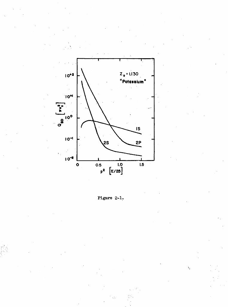
io*8
V10'
10-'
10"
Ze= 1.130
"Potassium1
0.5 1.0 1.5
Figure 2-1.
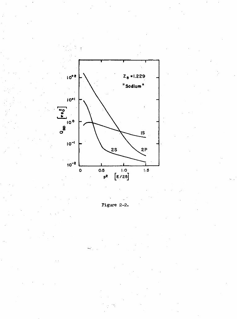
10*
10*'
NOo
L I*
10'S
10'
10"
Ze-1.229
"Sodium11
0.5 1.0 1.5
[E/ZS]
Figure 2-2.
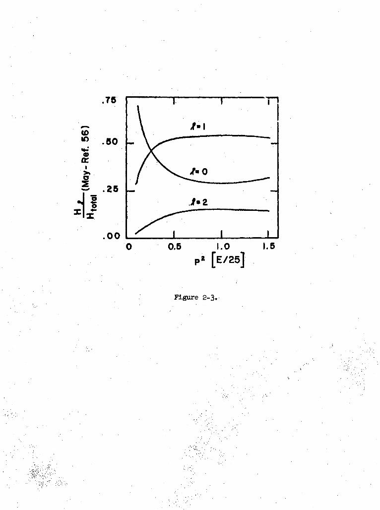
.75
<0.50
~ .25
.000.5 1.0 1.5
[E/25]
Figure 2-3.
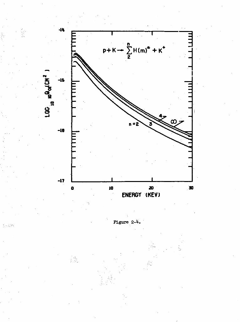
5 '-»-fc
-16
-1710 20
ENERGY (KEV)
Figure 2-U.
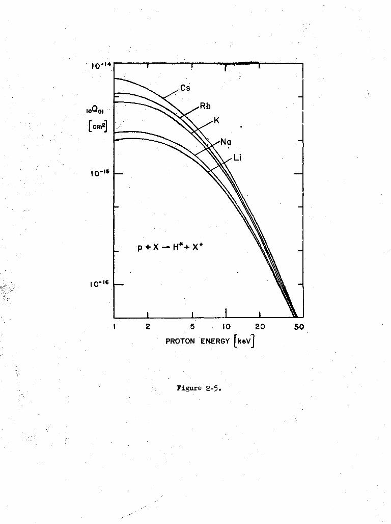
10-14
io-'8 -
IO'IB —
5 10 20
PROTON ENERGY [kev]
50
Figure 2-5.
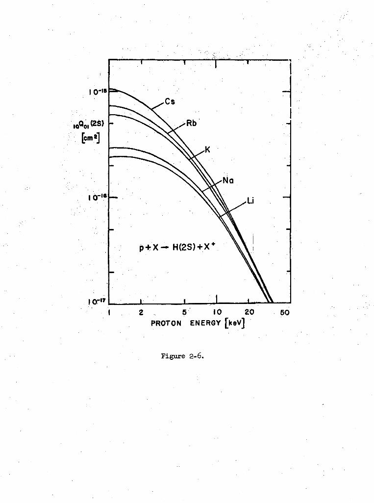
to-'
-Cs
-Rb
K
No
Li
- H(2S) + X*
2 5 10 20PROTON ENERGY [keV]
50
Figure 2-6.
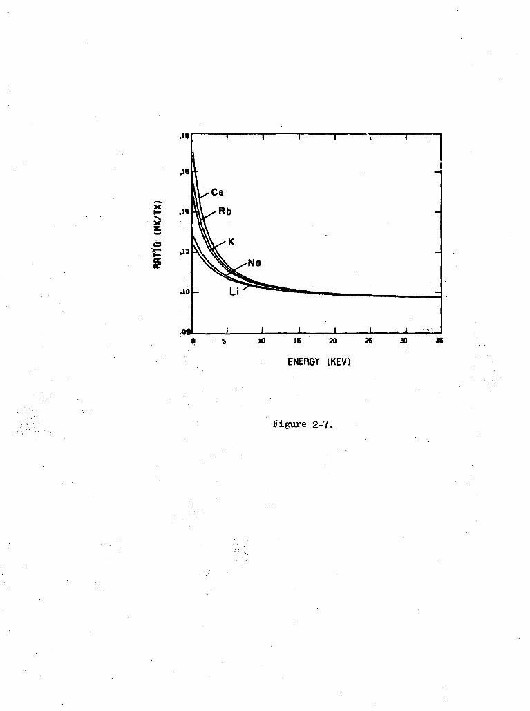
X
d
O S 1 0 1 5 2 0 2 5 3 0 3 5
Figure 2-7.
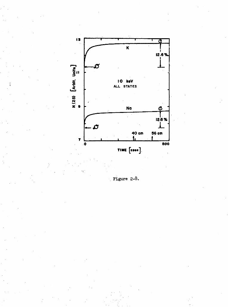
13
1"
1<
10 k«VALL STATES
12.6%.I
COCM^*z »
BOO
TIME
Figure 2-8.
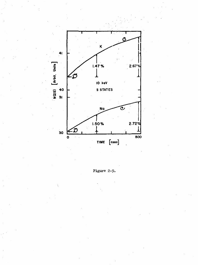
41
I 3,
30
I T
No
1
TIME [nsec]
500
Figure 2-9.
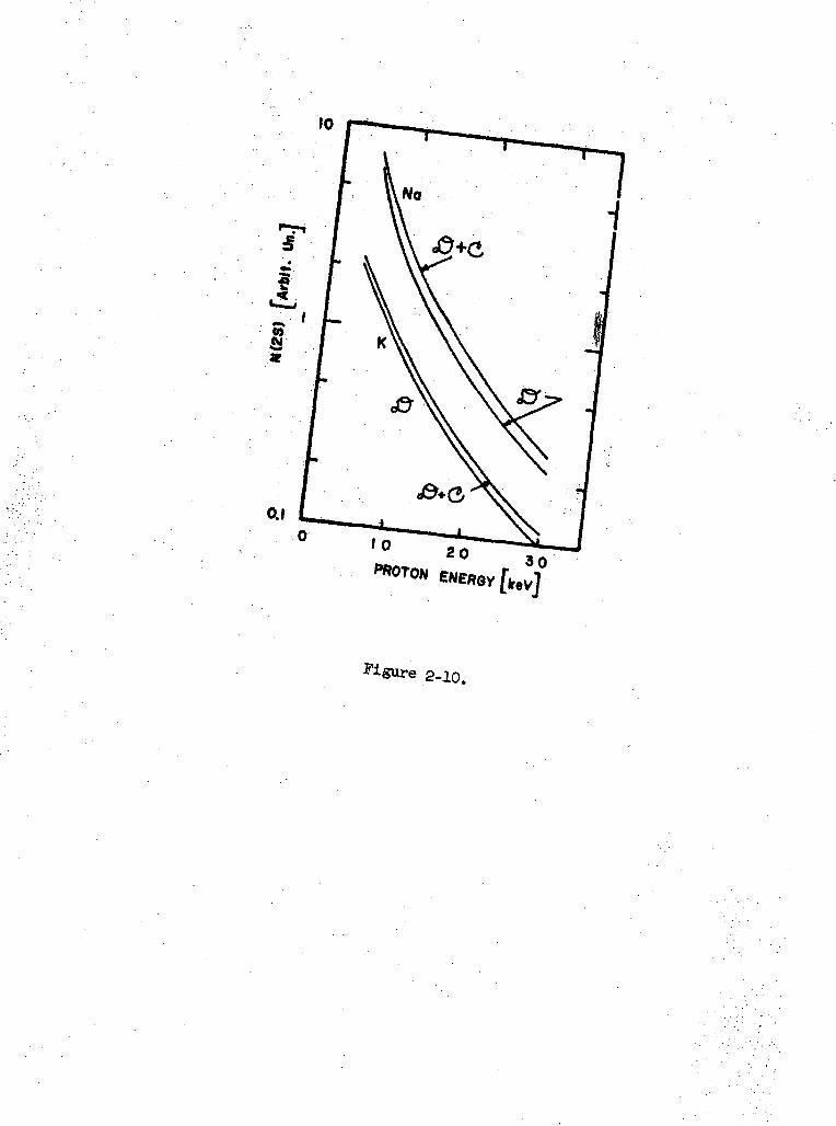
Figure 2-10.

HI
co0)
•H

FARADAY CUP GUARD
CURRENT -CARRYING
WIRE
CU / BRIDGEWIRE
0 1 2 3 c m FOIL
INSULATOR
Figure 3-2.

Figure 3-3.
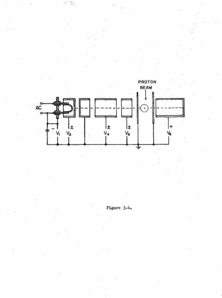
PROTONBEAM
o-, T
V4
+
V8
Figure 3-

4.0
8.0
2.0
1.0
T I I
O Wotonob*
• LM
I I1212
x [I]1222
Figure 3-5.

1-0
55V)
iV)
UJ
UJo:
01
0 01-0-8 0-0
[RADIANS]0-8
Figure 3-6.
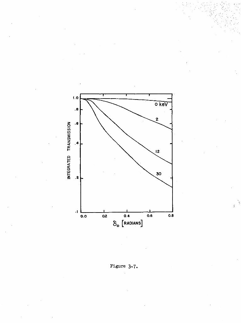
1.0
.8
.6V)en
V)zoc
QUJ
<rLJS .2
0.0 0.4 0.6
[RADIANS]
0.8
Figure 3-7.

38
v IO /l/aSource Press.- BO p. of H? 16 keV proiyus ov. NCI
3.0OSORS aoo /)$ 451 3? 5
Dtot Dn Dzero JT^ Tf Tm_^_Ta Ip
Scale 5 - Pos. VoHage ^ I T2
Total Flux Decreased 8 % Protonduring Mvasuremenr Current (/*A)
Figure lv-
as/.
. .Counter No. I - 1260 VDC
toMp"****,2.j?0 &-L Oxygen in filter
OSofiS °oo ft B 451 3i5 3?8 375<_~J 7-8- /O frlAto-aS-otto &30 .
\ Field Off Field On Beam Off\ Counts
Rod. SourceCalib.
Figure U~

10-14
[cm2]
10-15
10,-16
H*+K +
• This Work
o Il'in•*• Schmelzbach
- C = l-65
10 100
ENERGY [keV]
Figure 5-1.

10rl4
or10
[cm2]
10"
10"5 10 20
ENERGY [keV]50
Figure 5-2.

jo'1* i r r
10
10-"
.*.
JA T
1
"»«•I
10 20 30
ENERGY [ke\/J
Figure 5-3.
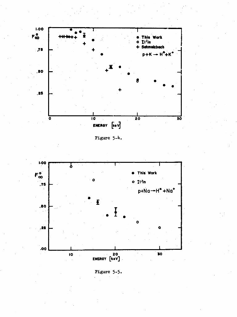
1.00
Froo
.00 .^_ , ,
t+ * . • ThU Worko
8 r 4- SchiMlzbach
p-FK •— H'-I-K1
• » ° h • • • • : • * * . - i• •
+.28
J10 20 30
ENCROY
Figure 5-4.
i ' . I
o • This Work
... ° o H'ln.«O "T • -
p+Na—H'-i-Nq*
.80
.26
.00
10 20ENERGY [k«V]
Figure 5-5.
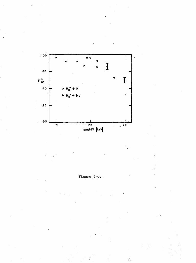
1.00
.75
00
.50
.25
• •O O •
o 1
o H2* + K
• H8*+ No
.00 I _—L10 2O
ENERGY [k«v]
3O
Figure 5-6.

icr18
0»
M
10
POTASSIUM
10 20
ENERGY [kev]
30
Figure 5-7.

10'
'01
lO'1
10
T < '
SODIUM
15 20
ENERGY [keV]
25
Figure 5-8.
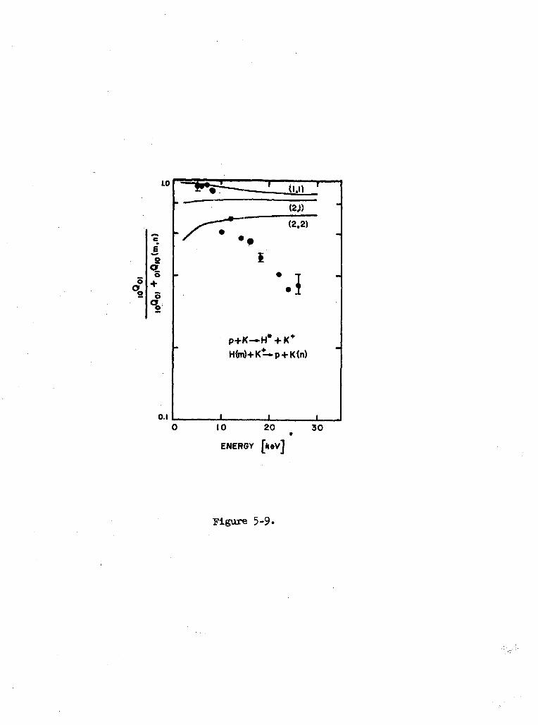
1.0
e6
(2.2)
p+K—H* + K*
O.I
10 20
ENERGY [heVJ
30
Figure 5-9.
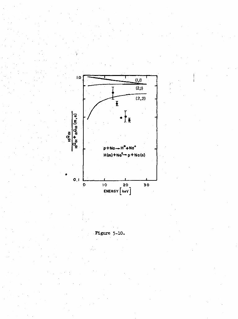
1.0
2q.
o°2 p+No—H*+No*
H(m)+No4—p+Na(n)
O.I _L
10 20
ENERGY [keVJ
30
Figure 5-10.

r
10-18
10'
Cs
(Det.Bal.)'
Rb
Li max. 8-7 (-18)I
5 10 20ENERGY [kev]
50 100
Figure 5-11.

10-14 fc=r
10-•• u
10 -16
Valence +Inner Shell
2 5 10 20
PROTON ENERGY [kev]
Figure 5-12.

10.-16
10
ENERGY [kev]
100
Figure 5-13.
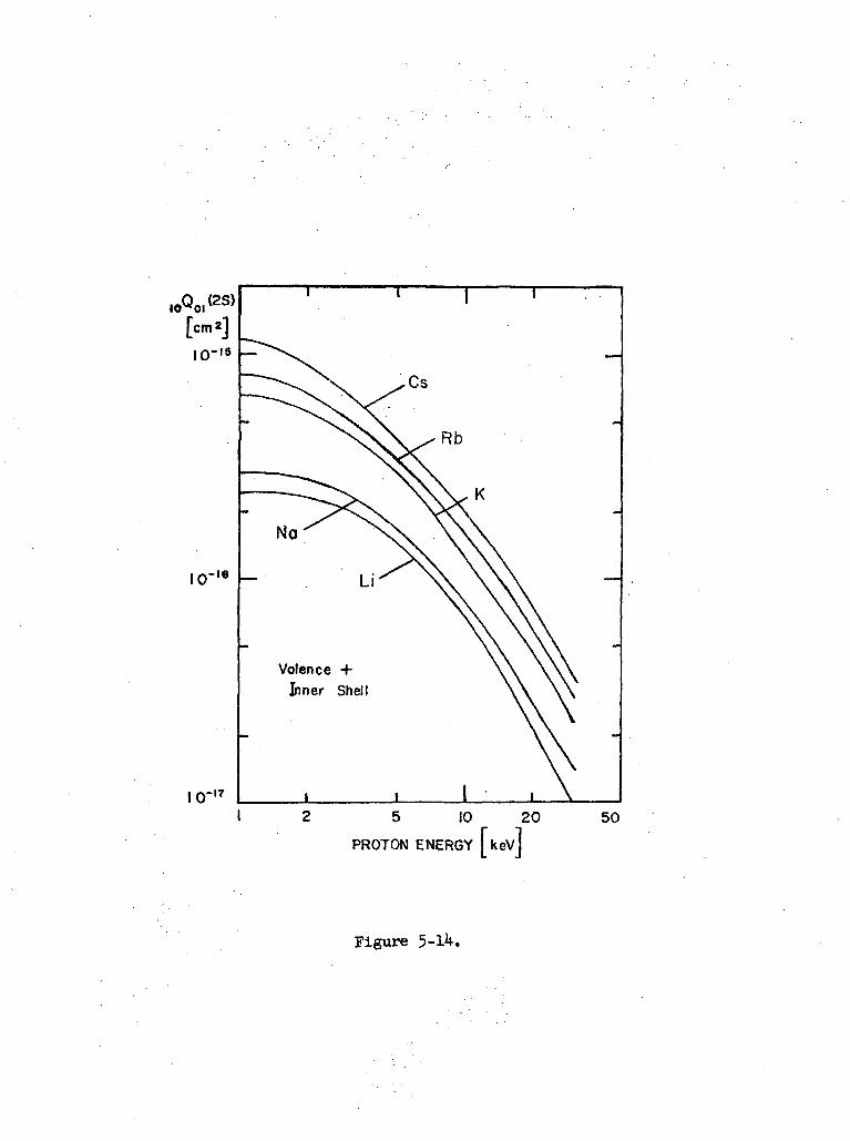
,oQo,(2S)
[cm*]10-15
10-16
10-17
Cs
Valence +Inner Shell
5 10
PROTON ENERGY [keVj
20 50
Figure 5-j
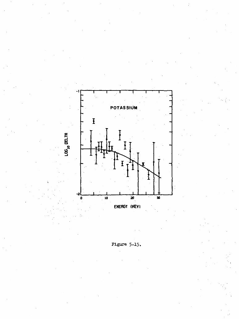
ia
8"
10 20 30
ENERGY (KEY)
Figure 5-15.

§
10 20
ENERGY (KEV)
Figure 5-16.

[AM]
30
20
10
• NO FIELD
o FIELD ON
x NEUTRALS
16 k*V
2 4 6 8x10"SODIUM DENSITY [cm**]
Figure 5-17.
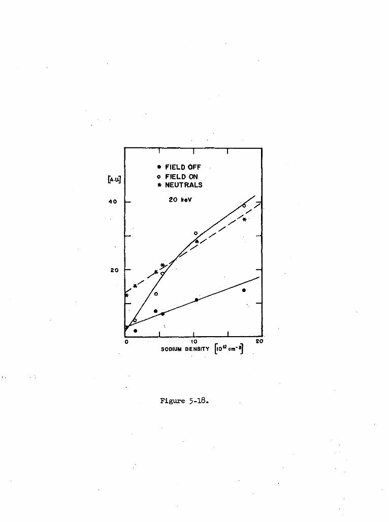
40
I I
• FIELD OFFo FIELD ON* NEUTRALS
20 keV
20
10SODIUM DENSITY fo'2om-»]
Figure 5-l8.

5
-te
-17
PnQTQN ON EXCITEDSODIUM AND POTflSSUW
No
I I I10 30
ENERGY (KEV)ao
Figure 5-19.
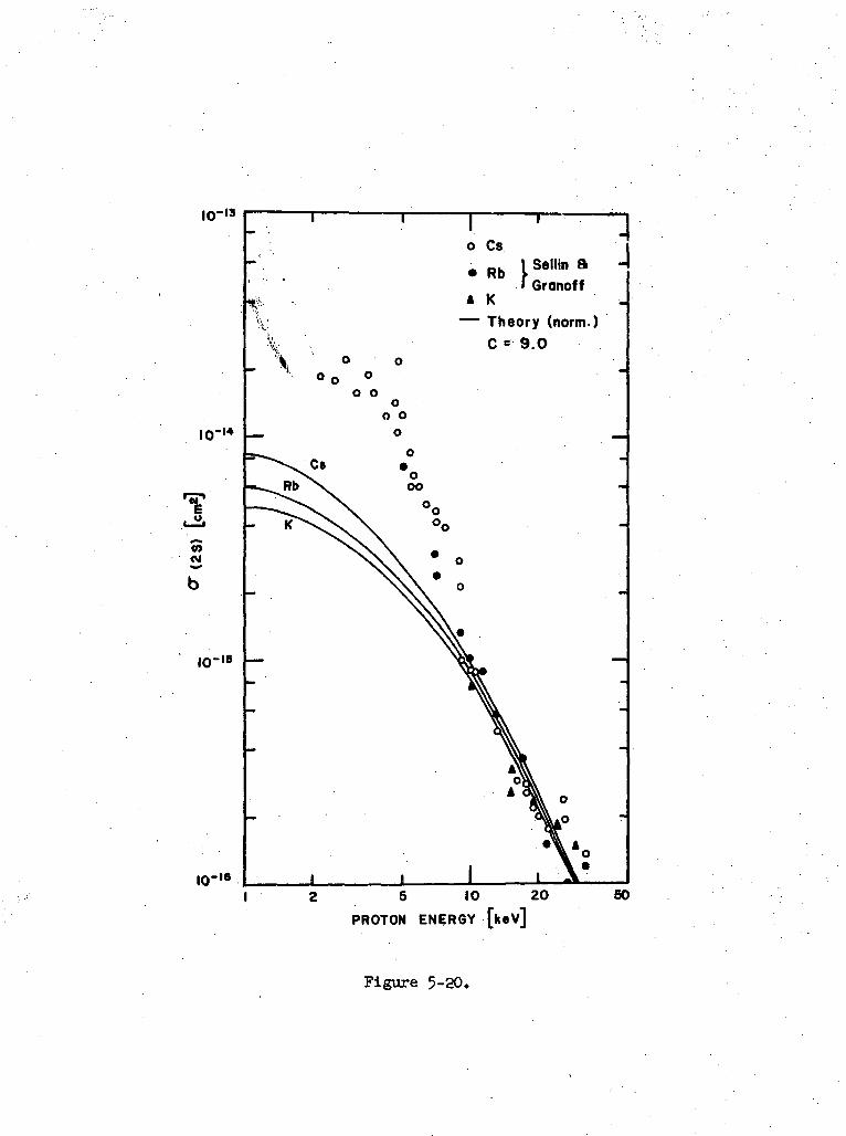
io-|S
10"'
m<M
io-|B
10-16
i \
o Cs
• Rb' Gronoff
A K— Theory (norm.)
C <* 9.0
o oo
o oo
5 10
PROTON ENERGY
20 50
Figure 5-20.
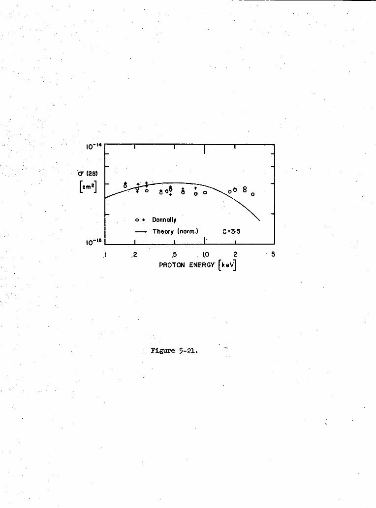
10"
<T(2S)
10-IB
6 8
o + Donnally
—r Theory (norm.)
.2 .5 1.0 2
PROTON ENERGY [kev]
Figure 5-21.
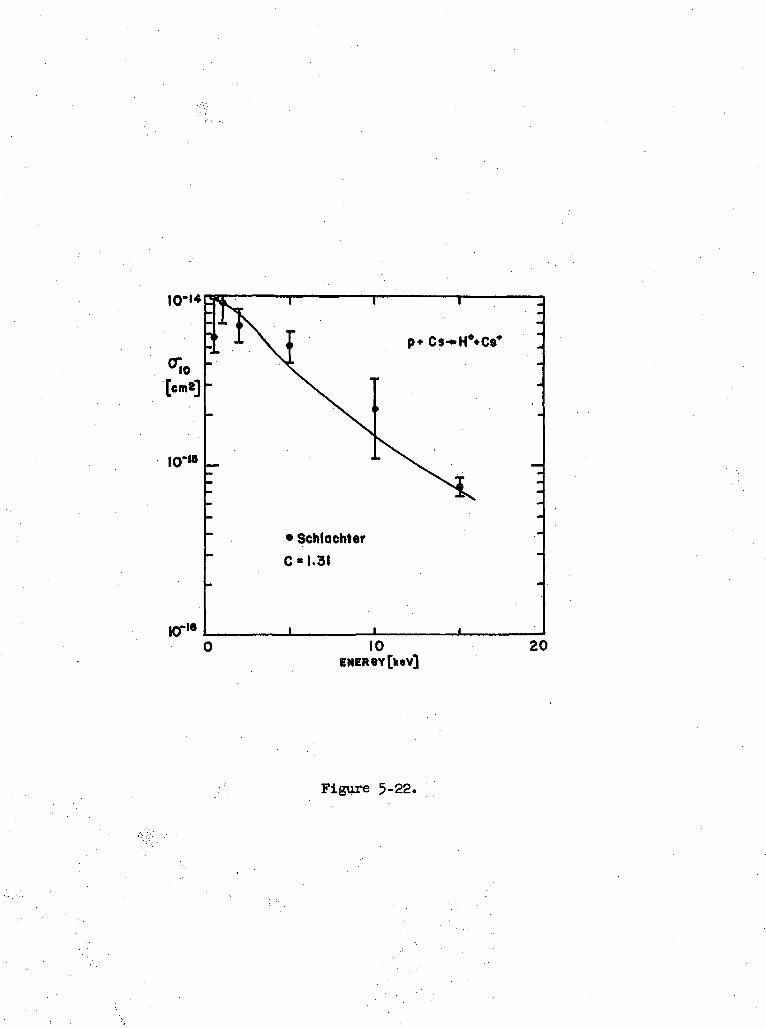
10-14
[erne]
• SchlaehterC-I .3I
10ENERGY [keV]
20
Figure 5-22.

1000
800
600
WO
I2"0
-200
-WO
-600
-800
-1000
a
0 1 2 3 1 5 6
ELECTRIC FIELD (KV/CM)
Figure C-l.
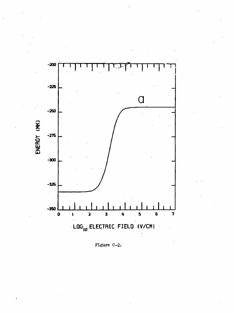
-200 T^T
-225
•250
a
-275
UJ
LU
-300
-325
-350 J L L[J J I I 111 III I I I
0 1 6
LOGW ELECTRIC FIELD (V/CN)
Figure C-2.
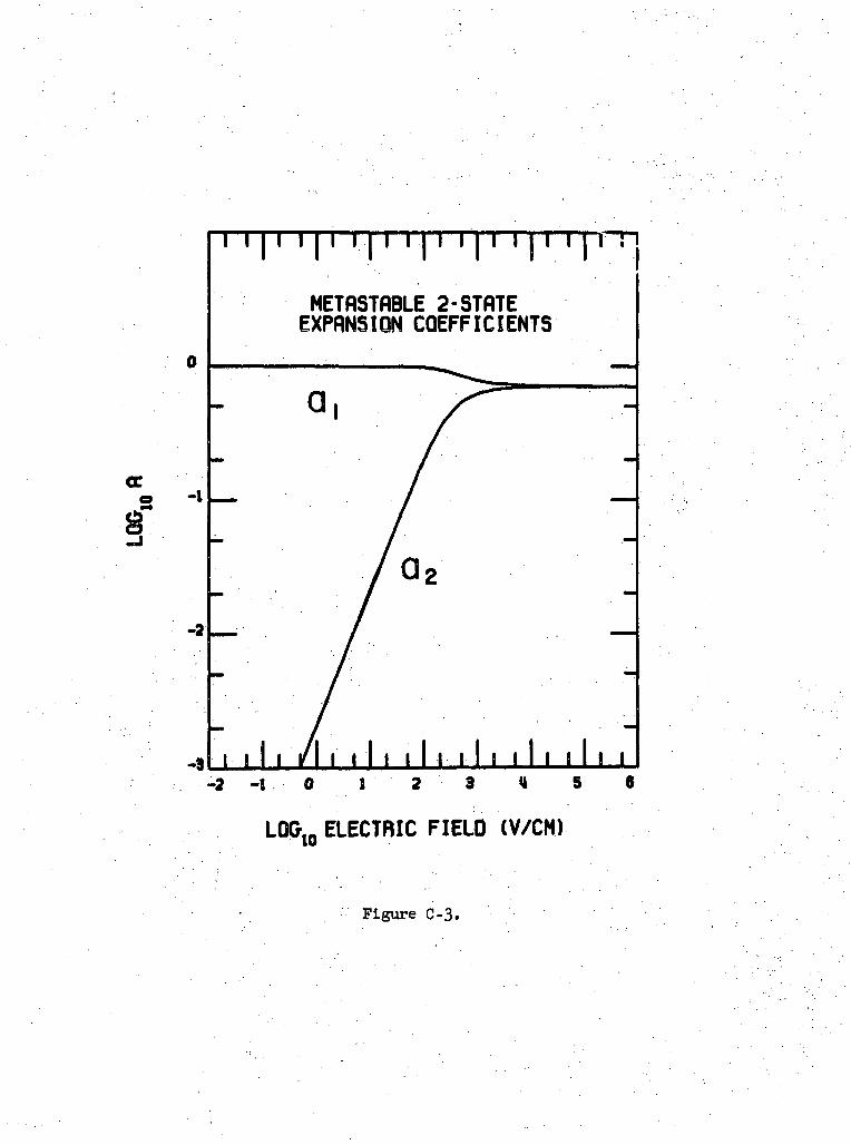
i ill MI ii i ill i I i i I i MI;
METflSTflBLE 2-STflTEEXPflNSIQN COEFFICIENTS
-i
I i .I. . I • i. 11. .I. . I- 2 - 1 0 1 2 3 U 5 6
L00lo ELECTRIC FIELD (V/CM)
Figure C-3.
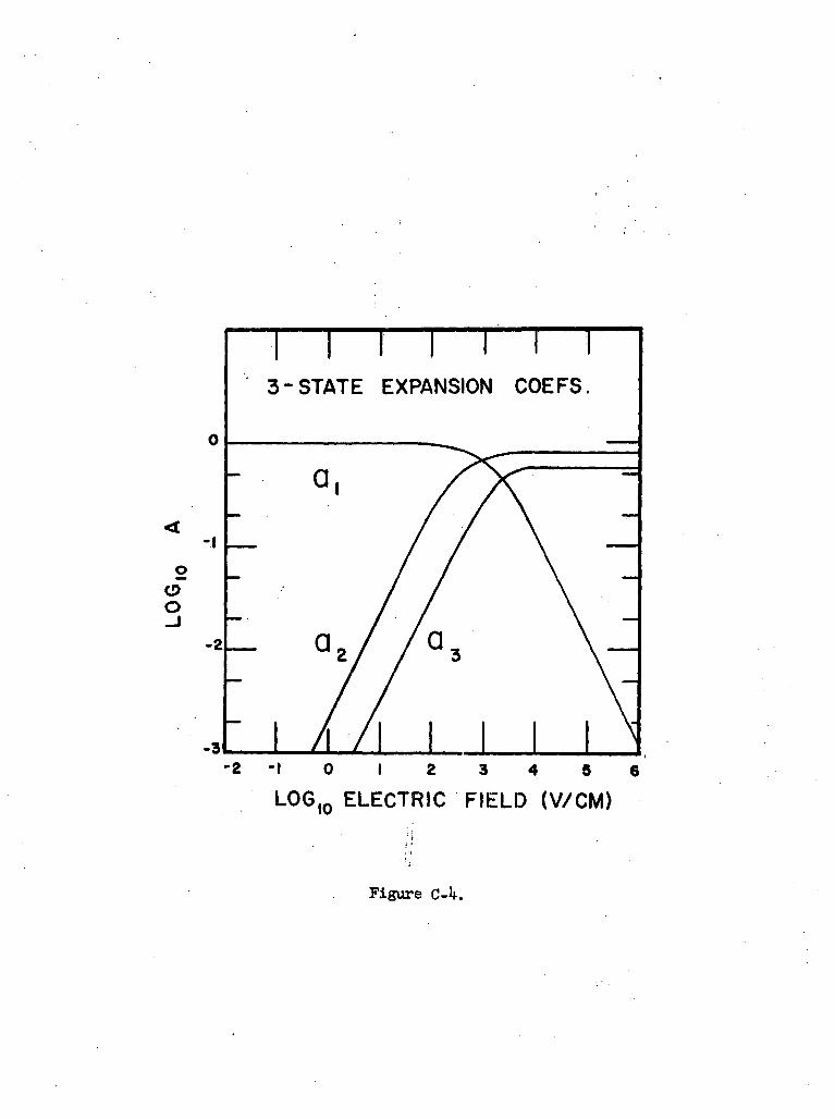
T i i3-STATE EXPANSION COEFS.
-io
C9~O
-2
-3
- 2 - 1 0 1 2 3 4 5 6
LOG|Q ELECTRIC FIELD (V/CM)
Figure C-k.
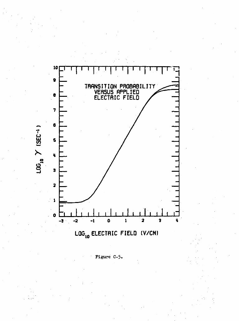
10
g
8
7
~ 67
a .
IIi I ii I i i I i i l l i l l i i i i_
TRRNSITIQN PRQBflBILITYVERSUS flPPLIEDELECTRIC FIELD
I t l I i i l l i l l i l l i '-3 -2 -1
LOG10 ELECTRIC FIELD (V/CM)
Figure C-5.

a
7 _
8 _
S .
a .
TRflNSITlQN PRQBRBILITYVERSUS flPPLIEOELECTRIC FIELD
5 6 70 1
LOGIO ELECTRIC FIELD (V/CM)
Figure C-6.
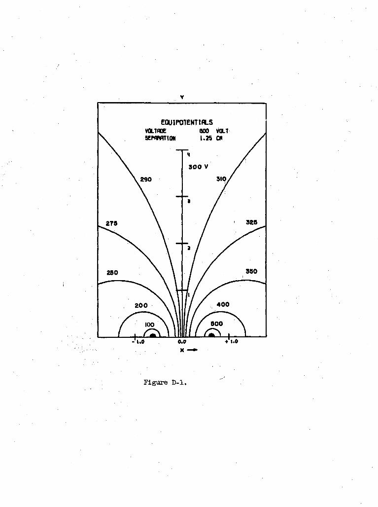
EQUIPQTENTIflLSVQLTAQE 600 VOLTSEWWION I.2S C*
Figure D-l.
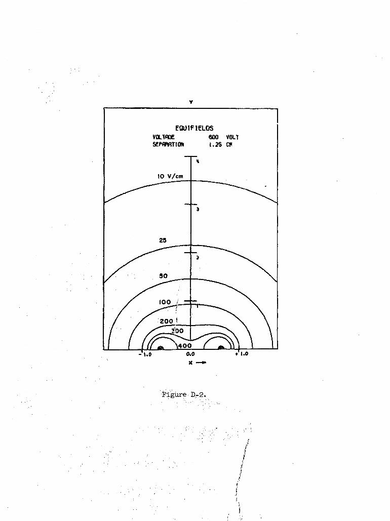
EQUIPIELOSVOLTAGE 600 VOLT
J.25 Cf!
•Figure D-.2..