The form and stability of alluvial

riverbeds, and their effects on

macroinvertebrate communities

across Great Britain

Rhodri J. Thomas

School of Biosciences

May 2018

Thesis submitted for the degree of

Doctorate of Philosophy

i

Declaration

This work has not been submitted in substance for any other degree or award at this or any other university or place of learning, nor is being submitted concurrently in candidature for any degree or other award.

Signed ………………………………………… (candidate) Date …..…….………

STATEMENT 1

This thesis is being submitted in partial fulfilment of the requirements for the degree of PhD.

Signed ………………………………………… (candidate) Date ……...……………

STATEMENT 2

This thesis is the result of my own independent work/investigation, except where otherwise

stated, and the thesis has not been edited by a third party beyond what is permitted by Cardiff

University’s Policy on the Use of Third Party Editors by Research Degree Students. Other

sources are acknowledged by explicit references. The views expressed are my own.

Signed ……………………….………….…… (candidate) Date …….……………

STATEMENT 3

I hereby give consent for my thesis, if accepted, to be available online in the University’s Open

Access repository and for inter-library loan, and for the title and summary to be made available

to outside organisations.

Signed …………………………..………..….. (candidate) Date …………………

STATEMENT 4: PREVIOUSLY APPROVED BAR ON ACCESS

I hereby give consent for my thesis, if accepted, to be available online in the University’s Open

Access repository and for inter-library loans after expiry of a bar on access previously

approved by the Academic Standards & Quality Committee.

Signed ………………………………..……… (candidate) Date ………….………

15th May 2018

15th May 2018

15th May 2018

15th May 2018

15th May 2018

ii

Acknowledgements

Firstly, I would like to thank my main supervisor, Dr Ian Vaughan, for his patience and

advice throughout my journey to being a reluctant ecologist. I would also like to thank

my co-supervisors, Prof Steve Ormerod and Dr Jose Constantine for their support,

guidance and general enthusiasm when tackling this often challenging, interdisciplinary

project. Thirdly, I would like to thank Dr Tano Gutierrez for his guidance on functional

ecology and the huge number of contributors to the datasets used in this thesis, without

whom these types of study would not be possible.

I thank my colleagues Huw, Josh, Alex and Scott, along with my informal supervisor, Dr

TC Hales in the Geomorphology group at the School of Earth & Ocean Sciences whose

shared experiences during our PhD’s have provided the motivation to complete this

thesis. I also thank family & friends who have been sounding boards, enthusiastic

listeners and distractions when I have wanted to discuss (or sometimes avoid

discussing…) my research.

Finally, I would like to thank my wife Steph, my mother, Sandra and my late father,

Martin, for their whole-hearted support throughout my PhD and without whom, I wouldn’t

have accomplished this work. This thesis is for you, Dad.

Funding for this thesis has been provided by a Presidents Research Scholarship from

Cardiff University.

The Centre for Ecology and Hydrology is thanked for providing flow data, the Environment

Agency, Natural Resources Wales and Scottish Environment Protection Agency are thanked for

providing access to the River Habitat Survey, WIMS and biological sampling network data. Marc

Naura is also thanked for providing access to site photos included in RHS. The RIVPACS data

collection, and compilation of the database, was funded by the Centre for Ecology and Hydrology,

Countryside Council for Wales, Department of the Environment, Food and Rural Affairs, English

Nature, Environment Agency, Environment and Heritage Service, Freshwater Biological

Association, Scotland and Northern Ireland Forum for Environmental Research, Scottish

Environment Protection Agency, Scottish Executive, Scottish Natural Heritage, South West

Water, Welsh Assembly Government.© NERC (CEH). 2006. Database right NERC (CEH) 2006.

All rights reserved.

All analyses were carried out using R version 3.01 (R Development Core Team, 2013).

iii

Table of Contents

Declaration ................................................................................................................... i

Acknowledgements ...................................................................................................... ii

Table of Contents ........................................................................................................ iii

List of Figures ..............................................................................................................vi

List of Tables ...............................................................................................................ix

Thesis summary ..........................................................................................................xi

1 General Introduction ........................................................................................... 12

Thesis aims ................................................................................................. 14

2 Literature Review: challenges and opportunities for linking physical habitat and

organisms in rivers ..................................................................................................... 16

Introduction .................................................................................................. 16

Controls on physical habitat ......................................................................... 17

Different approaches for linking physical habitat and species’ distributions .. 20

The role of species traits .............................................................................. 23

Methods for predicting bedform distribution and bed disturbance ................ 25

Climate change and the need for better prediction ....................................... 28

Nationwide datasets and the emergence of river restoration in the UK ........ 30

Conclusions ................................................................................................. 32

3 Controls on the spatial distribution of bars within the alluvial rivers of Great Britain

33

Abstract ....................................................................................................... 33

Introduction .................................................................................................. 34

Methods....................................................................................................... 36

3.3.1 RHS ...................................................................................................... 36

3.3.2 Discharge Estimation ............................................................................ 37

3.3.3 Substrate Size ...................................................................................... 38

3.3.4 Specific Stream Power ......................................................................... 38

3.3.5 Statistical Methods ............................................................................... 38

Results & Discussion ................................................................................... 40

iv

3.4.1 National controls on bar distribution ...................................................... 40

3.4.2 Critical Specific Stream Power .............................................................. 45

3.4.3 Regional controls on bar distribution ..................................................... 46

Conclusion ................................................................................................... 50

Appendix ..................................................................................................... 51

4 Effects of bed composition and stability on river invertebrates ............................ 53

Abstract ....................................................................................................... 53

Introduction .................................................................................................. 54

Methods....................................................................................................... 59

4.3.1 RIVPACS dataset ................................................................................. 59

4.3.2 Invertebrate Traits ................................................................................ 61

4.3.3 Geomorphic Template .......................................................................... 63

4.3.4 Data analysis ........................................................................................ 66

Results ........................................................................................................ 72

4.4.1 Community metrics ............................................................................... 73

4.4.2 Functional diversity ............................................................................... 75

4.4.3 Individual resistance/resilience traits ..................................................... 78

4.4.4 Feeding guilds and locomotory traits .................................................... 85

Discussion ................................................................................................... 87

4.5.1 Limitations ............................................................................................ 87

4.5.2 Effects of disturbance and substrate type on invertebrate community

composition and function .................................................................................... 90

4.5.3 Trophic relationships ............................................................................ 93

Conclusion ................................................................................................... 94

Appendix ..................................................................................................... 95

5 Benthic invertebrate response to riverbed disturbance ....................................... 97

Abstract ....................................................................................................... 97

Introduction .................................................................................................. 98

Methods..................................................................................................... 103

5.3.1 Data Sources ...................................................................................... 103

v

5.3.2 Macroinvertebrate data ....................................................................... 103

5.3.3 Daily river flows .................................................................................. 104

5.3.4 Water quality ...................................................................................... 105

5.3.5 River Habitat Survey ........................................................................... 105

5.3.6 Site Selection ..................................................................................... 106

5.3.7 Data Analysis ..................................................................................... 107

Results ...................................................................................................... 113

5.4.1 Spatial distribution of disturbance ....................................................... 113

5.4.2 Site-level (cross-sectional) analysis of invertebrate community response

to bed disturbance ............................................................................................ 115

5.4.3 Longitudinal analysis 1: The role of disturbance in summer versus winter

118

5.4.4 Longitudinal analysis 2: Interaction between water quality improvements

and disturbance ................................................................................................ 119

Discussion ................................................................................................. 121

5.5.1 Limitations .......................................................................................... 121

5.5.2 Spatial trends in disturbance............................................................... 123

5.5.3 Evidence for invertebrate community response to disturbance ........... 124

Conclusion ................................................................................................. 126

Appendix ................................................................................................... 127

6 General Discussion ........................................................................................... 129

Synthesis ................................................................................................... 129

6.1.1 Overview ............................................................................................ 129

6.1.2 The distribution of physical habitats .................................................... 130

6.1.3 Process-based models linking habitat with community composition .... 131

6.1.4 The temporal role of disturbance ........................................................ 131

Implications ............................................................................................... 132

Limitations ................................................................................................. 135

Future areas of study ................................................................................. 136

Conclusion ................................................................................................. 138

7 References ....................................................................................................... 139

vi

List of Figures

Figure 2-1: Conceptual diagram showing the key controls placed on the abundance

and diversity of stream organisms and how those controls interact. ........................... 18

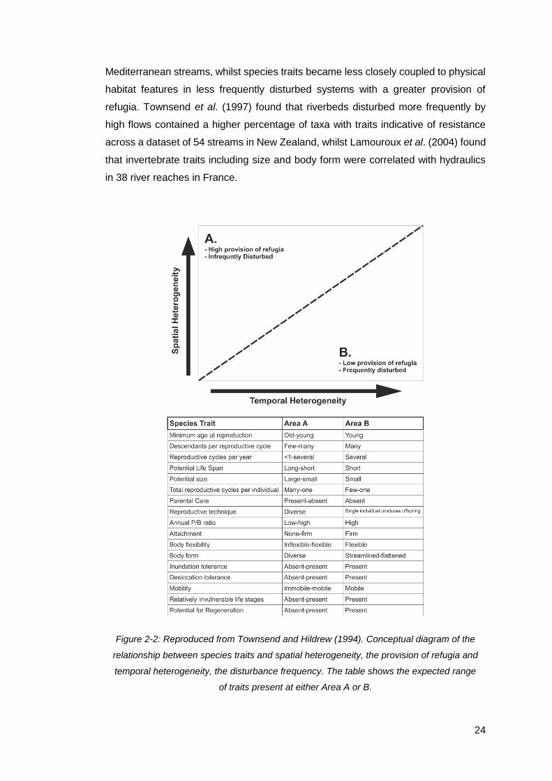
Figure 2-2: Reproduced from Townsend and Hildrew (1994). Conceptual diagram of

the relationship between species traits and spatial heterogeneity, the provision of

refugia and temporal heterogeneity, the disturbance frequency. The table shows the

expected range of traits present at either Area A or B. ............................................... 24

Figure 2-3: A conceptual diagram of the progression of development of a simple

method for predicting the frequency of disturbance at a location. Explanatory power, in

terms of process, is increased with the addition of the mode of sediment transport. The

simple variables required for each method are included. ........................................... 28

Figure 3-1: Distribution of the 1480 RHS sites used in the study on (A) a map of Britain

and (B) the D50-ω axes. The grey, dashed line is a convex hull that incorporates all

RHS sites................................................................................................................... 40

Figure 3-2: The probability of occurrence of (A) all bar types, (B) point bars, (C)

alternate bars and (D) mid-channel bars are modelled using general additive models

on the D50-ω axes. The colour-bars indicate areas of low-high probability of bar

occurrence. ................................................................................................................ 42

Figure 3-3: Interpolated maps of the probability of bar occurrence, as modelled on the

D50- axes, for (A) all bar types, (B) point bars, (C) alternate bars and (D) mid-

channel bars. The colours indicate areas of low-high probability of bar occurrence. .. 43

Figure 3-4: (A) Interpolated map of model residuals scores denoting the success of the

D50- model of all three bar types. A score near to zero indicates good agreement

between predicted probabilities and bar presence/absence, whereas scores closer to -

1 or 1 indicate over- or under-estimates of bar prevalence respectively. (B)

Interpolated map of the extent of bank modification. The colours indicate the

percentage of bank length within each RHS site that has been noticeably modified. . 48

Figure 3-5: (A) Percentage of RHS sites characterized by rock type based on the

mean predicted probability of the D50- model (expected) compared to the mean

probability of the actual values (observed). RHS sites with bars present that were

poorly predicted by the model (residual >0.5) are split from RHS sites with bars that

were well-predicted (residuals <0.5) to highlight that poorly predicted sites are more

likely to have (B) emergent marginal macrophytes present and (C) a substrate

composed of clay, silt or sand. ................................................................................... 49

vii

Figure 3-6: The probability of occurrence of (A) all bar types, (B) point bars, (C)

alternate bars and (D) mid-channel bars for the range of specific stream power values

at the mid-point of each substrate type along with the standard error of each

prediction. The dashed black line indicates the identified threshold ω of 30 W m-2..... 51

Figure 3-7: The predicted probability of occurrence of (A & B) point bars, (C & D)

alternate bars and (E & F) mid-channel bars at minimum (A, C, E) and maximum (B,

D, F) channel modification. ........................................................................................ 52

Figure 4-1: Predicted effects of increased riverbed disturbance on functional diversity

indices in multidimensional functional space (two dimensions are shown here for

simplicity). Each point represents one taxon, plotted according to its trait values, with

point diameter proportional to taxon abundance. Functional richness (FRic) is

calculated as the size of the convex hull that encapsulates all of the points in space,

and is independent of abundance. Functional evenness (FEve) uses the minimum

spanning tree (dashed line) to measure the regularity between point spacing and size

(i.e. abundance) along the tree. Functional dispersion (FDis) measures the overall

distance of all taxa from the centroid of the community and is weighted by abundance.

Increased disturbance is expected to result in lower FRic (i.e. a smaller convex hull),

higher FEve (i.e. more regular spacing and size along the minimum spanning tree) and

lower FDis (i.e. a lower mean distance to the centroid) (Legendre and Legendre, 1998;

Villeger et al., 2008). .................................................................................................. 69

Figure 4-2: (A) A map showing the location of the 714 RIVPACS sites used in the

study. The bias towards upland rivers, due to the requirement for relatively pristine

watercourses, is evident. (B) The same 714 RIVPACS sites plotted on the Shields

Regime Diagram. The black line denotes a laboratory defined threshold for the

initiation of bed load motion of sediment (Parker et al., 2003), whilst the dotted black

line represents the threshold for suspended-load transport (Dietrich, 1982). .............. 72

Figure 4-3: The community metrics of species richness (A & B), abundance (C & D)

and rarefied richness (E & F) are plotted as Generalised Additive Models on the

Shields Regime Diagram (left) with slices through the models plotted against the y-

axes of the Shields Regime Diagram (right), which represents the propensity for

riverbed disturbance in the form of sediment transport. The coloured lines and error

bars denote slices taken through the GAM at cobble (red), gravel (blue), sand (orange)

and silt (purple) substrates. ........................................................................................ 74

Figure 4-4: The metrics of functional richness (FRic; A & B) and functional dispersion

(FDis; C & D) are plotted as Generalised Additive Models on the Shields Regime

Diagram (left) with slices through the models plotted against the y-axes of the Shields

Regime Diagram (right), which represents the propensity for riverbed disturbance in

the form of sediment transport. The coloured lines and error bars denote slices taken

viii

through the GAM at cobble (red), gravel (blue), sand (orange) and silt (purple)

substrates. ................................................................................................................. 76

Figure 4-5: Null models of functional richness (A & B; ses.FRic) and functional

dispersion (C & D; ses.FDis) are plotted as Generalised Additive Models with a

diverging colour gradient on the Shields Regime Diagram (left). The dashed grey lines

are thresholds of +/- 0.2 which indicate the approximate 5% significance level and are

deemed as significantly different to the random expectation (Mason et al., 2013).

Slices through the models are plotted against Dimensionless Shields Number (right)

which represents the propensity for riverbed disturbance in the form of sediment

transport. The coloured lines and error bars denote slices taken through the GAM at

cobble (red), gravel (blue), sand (orange) and silt (purple) substrates. ...................... 77

Figure 4-6: The proportion of an invertebrate community with lifespans of (A) <1 year

and (B) >1 year, plotted against a measure of propensity for disturbance

(Dimensionless Shear Stress - τ*). The coloured lines and error bars denote slices

taken through the GAM at cobble (red), gravel (blue), sand (orange) and silt (purple)

substrates. ................................................................................................................. 79

Figure 4-7: The proportion of an invertebrate community with dispersal methods of (A)

aquatic passive and (B) aerial active, plotted against a measure of propensity for

disturbance (Dimensionless Shear Stress - τ*). The coloured lines and error bars

denote slices taken through the GAM at cobble (red), gravel (blue), sand (orange) and

silt (purple) substrates................................................................................................ 80

Figure 4-8: The proportion of an invertebrate community with aquatic stages of (A)

lava and (B) adult, plotted against a measure of propensity for disturbance

(Dimensionless Shear Stress - τ*). The coloured lines and error bars denote slices

taken through the GAM at cobble (red), gravel (blue), sand (orange) and silt (purple)

substrates. ................................................................................................................. 81

Figure 4-9: The proportion of an invertebrate community with reproduction method of

(A) ovoviviparity, (B) isolated cemented eggs and (C) clutches – cemented or fixed,

plotted against a measure of propensity for disturbance (Dimensionless Shear Stress -

τ*). The coloured lines and error bars denote slices taken through the GAM at cobble

(red), gravel (blue), sand (orange) and silt (purple) substrates. .................................. 82

Figure 4-10: The proportion of an invertebrate community with reproductive cycles of

(A) <1 cycle p/y, (B) 1 cycle p/y and (C) >1 cycle p/y, plotted against a measure of

propensity for disturbance (Dimensionless Shear Stress - τ*). The coloured lines and

error bars denote slices taken through the GAM at cobble (red), gravel (blue), sand

(orange) and silt (purple) substrates. ......................................................................... 84

Figure 4-11: The proportion of an invertebrate community with locomotion methods of

(A) crawler and (B) burrower, plotted against a measure of propensity for disturbance

ix

(Dimensionless Shear Stress - τ*). The coloured lines and error bars denote slices

taken through the GAM at cobble (red), gravel (blue), sand (orange) and silt (purple)

substrates. ................................................................................................................. 85

Figure 4-12: The proportion of an invertebrate community with feeding methods of (A)

absorber, (B) shredders and (C) scrapers, plotted against a measure of propensity for

disturbance (Dimensionless Shear Stress - τ*). The coloured lines and error bars

denote slices taken through the GAM at cobble (red), gravel (blue), sand (orange) and

silt (purple) substrates................................................................................................ 86

Figure 5-1: Fuzzy correspondence analysis of the 877 samples based on the five

resistance/resilience trait categories (18 individual traits; Table 5-2). ....................... 110

Figure 5-2: (A to D) Spatial distributions of four disturbance metrics calculated based

on daily flow data and exceedance of the critical specific stream power threshold

(Parker et al., 2011). ................................................................................................ 114

Figure 5-3: Predicted linear trends of the means per site of (A) resistance trait gradient

(RS1), (B) taxon richness and (C) Jaccard dissimilarity index during the early (red) and

late (blue) time periods with decreasing disturbance. Water quality held constant

(mean values). Linear trends in (A) and (B) are non-significant (but included for

interpretation), whilst the late trend in (C) is significant at p<0.01............................. 116

Figure 5-4: GAMM predictions for trends in resistance trait gradient (RS1) versus (A)

summer and (B) winter disturbance, and Jaccard dissimilarity index versus (A)

summer and (B) winter disturbance. Random effects are set to zero. ...................... 119

Figure 5-5: GAMM predictions for trends in (A) resistance trait gradient (RS1), (B)

taxon richness and (C) Jaccard dissimilarity index for good (red) and poor (blue) water

quality with increasing disturbance (x axis). Random effects are set to zero. ........... 120

List of Tables

Table 3-1: C Index (predictive ability) scores for the models used in the study. Initially

models were split into bar types and whether vegetation was present or absent. The

frequency of results for each category along with the percentage of the dataset that

they represent is also shown. .................................................................................... 41

Table 3-2: Equations for critical specific stream power as produced in Petit et al.

(2005), Ferguson (2005) and Parker et al. (2012) and the predicted grain size of

material entrained by a flow with a specific stream power of 30 W m-2. The values for

Di and Db in Ferguson’s (2005) equation were taken as equal, despite there being a

difference between the size of material in transport and the dominant bed material in

alluvial rivers with mixed beds. ................................................................................... 46

x

Table 4-1: Chemical and physical variables from the RIVPACS dataset used to

describe each sampling location. Details of the measurement methods taken from

UKTAG (2008). .......................................................................................................... 60

Table 4-2: Eight candidate ecological traits (37 individual categories) for

resistance/resilience to bed disturbance and two additional traits (16 categories) for

invertebrate locomotion and feeding methods. Trait data from Tachet et al. (2002). .. 62

Table 4-3: Individual and groups of traits, as described in Tachet et al. (2002), shown

with R2 values for fitted models of each trait or mean values for each trait grouping (in

brackets). R2 values in bold indicate the traits with the strongest affinities (>0.2) to the

geomorphic template used in the model whose trends are described in Section 4.4.3.

.................................................................................................................................. 67

Table 4-4: Statistical significance (P-values) for the three smoothing terms and overall

model Rr used to model community and functional metrics in the GAMs ................... 95

Table 4-5: Statistical significance (P-values) for the three smoothing terms and overall

model R2 used to model individual traits in the GAMs ................................................ 96

Table 5-1: Five candidate ecological traits (21 individual categories) for

resistance/resilience to bed disturbance. ................................................................. 104

Table 5-2: Loading coefficients for the first two axes of a fuzzy correspondence

analysis conducted on the five resistance/resilience trait categories (18 individual

traits). Three reproduction categories (asexual, terrestrial, in vegetation) were

excluded due to low proportions skewing the FCA. .................................................. 111

Table 5-3: Axes loadings and variance explained for a PCA of the metrics used to

classify disturbance. ................................................................................................ 115

Table 5-4: Linear regressions of (A) the resistance trait gradient (RS1), (B) taxon

richness and (C) Jaccard dissimilarity index against disturbance and water quality

variables for the early and late periods. Estimated coefficients, their standard errors

and statistical significance from the models are shown. Significant predictors are in

bold. * indicates predictor variables that were log transformed to meet model

expectations. ........................................................................................................... 117

Table 5-5: The 78 invertebrate families used for the analysis. Taxon list matches

Vaughan and Ormerod (2014). Families with a * had missing trait information and were

excluded from the study. .......................................................................................... 127

Table 6-1: A summary of the process-based models used in this study, with their data

requirements, advantages, limitations and potential applications. ............................ 134

xi

Thesis summary

The sustainable functioning of macroinvertebrate communities forms the basis of many

of the vital ecosystem services provided by rivers, yet these communities are amongst

the most stressed on the planet and predictions show these stresses increasing in the

future. At a conceptual level, macroinvertebrate community composition is inextricably

linked to the riverbed sediment in which they reside, although evidence of these links is

largely confined to descriptive or small-scale studies. Robust predictions of the response

of these communities to future change are urgently needed but this first requires a better

understanding of the interaction between physical and ecological processes across

larger spatial and temporal scales.

Using national scale monitoring data for rivers across Great Britain, this study tested the

ability of simple process-based models to predict physical habitat features (e.g. bars),

before investigating their ability to describe spatial and temporal trends of invertebrate

community function, composition and response to physical perturbation. The simple

nature of the approaches used in this study, which combine basic geomorphological

models with traditional ecological metrics and functional traits, presents an opportunity

to develop tools that allow river managers to base decisions on quantifiable measures

of physical process instead of expert opinion.

Overall, the results provided evidence of an implicit link between freshwater community

composition, function, and the spatial variation in physical processes. Traditional and

functional measures of community diversity showed a response to changing bed

material calibre and stability across large spatial scales, consistent with other studies of

habitat stability in rivers and other ecosystems. Despite this, there was limited evidence

of temporal variability in communities due to riverbed disturbance, perhaps because

water quality continued to suppress the physical habitat signal. Further work is required

to isolate the effect of riverbed disturbance from other controlling mechanisms.

12

1 General Introduction

Freshwaters, including rivers, are amongst the most biodiverse ecosystems,

supporting an estimated 6% of all known species, despite covering only 0.8% of the

Earth’s surface (Dudgeon et al., 2006). At the same time, rivers provide hugely valued

ecosystem services to humans, such as drinking water, irrigation, recreation and

transport (Cotanza et al., 1997; Cotanza et al., 2014; Maltby et al., 2011). Human

activities have directly (e.g. through impoundment, abstraction and flood control) and

indirectly (e.g. through climate change and land use change) made rivers amongst

the most impacted and threatened ecosystems (Sala et al., 2000; Dudgeon et al.,

2006), and their long-term prognosis is poor as population growth and urbanisation

exacerbate these pressures on river systems (Palmer et al., 2008; Vorosmarty et al.,

2010). To address the consequences of these pressures, and improve river

management and restoration, a better understanding is required of the factors

shaping riverine biodiversity, species distributions and community structure (Petts,

2009). This cuts across traditional research disciplines including freshwater ecology,

geomorphology and hydrology, and emphasises the urgent need for more

multidisciplinary research (Dollar et al., 2007; Vaughan et al., 2009).

Physical habitat is considered to be one of the major drivers of biodiversity patterns

in rivers (Vannote et al, 1980; Townsend and Hildrew, 1994; Benda et al, 2004). Yet

despite its recognised importance and long history of research (e.g. Riley, 1921;

Percival and Whitehead, 1929), it has been comparatively understudied, primarily due

to a focus on water quality (Vaughan et al., 2009). In rivers, physical habitat is shaped

by the local movement of sediment, which in turn is largely controlled by four key

elements; sediment supply, sediment calibre, discharge and channel slope (Knighton,

1998). These parameters can be viewed as driving forces (discharge and slope) and

resisting forces (sediment calibre and supply) and they define the channel

morphology, the threshold at which sediment transport occurs and how the sediment

is transported through the channel. These processes create and redistribute the

habitats familiar to river ecologists e.g. riffles, areas of fine sediment or those suitable

for macrophyte colonisation (Demars et al., 2012). In theory, it should be possible to

predict how a river functions at a location based on an understanding of these key

parameters, creating scope for relatively simple process-based models that could be

linked to the ecology. Furthermore, capturing the dynamics of sediment transport

should help to describe the disturbance regime to which organisms are exposed

13

(Death and Winterbourn, 1995; Death, 2002; Schwendel et al., 2010a), which may

play an important role in determining community structure (Connell, 1978; Miller et al.

2010). These events alter the physical attributes of the channel and its instream and

riparian habitats, in turn impacting on the biota that reside in this altered habitat

(Death and Winterbourn, 1995; Death, 2002; Schwendel et al., 2010a), the subject of

this thesis.

Three major factors have contributed to a surge of interest in physical habitat over

recent years. Firstly, conservation and restoration efforts have successfully focussed

on improving water quality and have resultantly promoted the issues caused by

physical modifications and poor habitat quality to the fore of river restoration efforts

(Collins et al., 2012). Secondly, policy drivers such as the Water Framework Directive

(2000) have emphasised the importance of hydromorphology by placing it alongside

the traditional measures of riverine health, biological and water quality (Griffiths,

2002). Whilst this policy change has led to the consideration of hydromorphology by

the statutory bodies and other river managers, interdisciplinary research has been

slow to react and as such there is a lack of tools to pinpoint where ecology-

hydromorphology interactions can be improved (Vaughan et al., 2009). The third

factor is climate change, with predictions of changes in the timing, intensity and

overall magnitude of rainfall (Murphy et al., 2009; Kendon et al., 2014), with potential

ramifications for physical habitat. Climate is a major control on the flow regime of the

stream network (Poff et al, 1997), the production and delivery of sediment (e.g. by

triggering landslides; Parker et al., 2016) and land use (e.g. by controlling the

distribution of vegetation; Bachelet et al, 2001), which in turn control smaller scale

variations including reach-scale morphology (Buffington and Montgomery, 1997) and

water temperature (van Vliet et al., 2013). Climate is a major control on sediment

supply to the fluvial network over long timescales, especially in regions with little

tectonic activity such as the UK, with both the frequency and intensity of storm events

influencing rates of sediment delivery to river channels via hillslope processes (Wilby

et al., 1997). General predictions of more frequent and intense storm events across

the UK in coming decades as well as changes in overall precipitation trends have

created the need for initial understanding and eventual prediction of the likely changes

to both physical habitats and the organisms residing within them.

Against this background of greater interest, there are great challenges but also great

opportunities. Traditional approaches are challenged by interdisciplinary study and

the need to account for changing conditions. Current ecological models are static and

14

correlative, making them poor at extrapolating beyond the conditions under which

they were calibrated (Urban et al., 2016). To reliably model changing conditions, such

as the likely changes in sediment supplies and flow regimes as a result of climate or

land use change, a shift to process-based modelling is needed (Urban et al., 2016,

Zurell et al., 2016). Another consideration is that of scale. River managers require

insight at sufficient scales (i.e. catchment or greater) but datasets that provide this

coverage are typically too expensive or time consuming to collect by field study so

novel use of existing datasets or rapid collection techniques are needed (Carbonneau

et al., 2012). The UK is uniquely positioned to address these challenges due to its

extensive biological and chemical monitoring networks, gauging stations and physical

habitat classifications (Vaughan and Ormerod 2010).

Thesis aims

The need for greater understanding of the interactions between freshwater ecology

and hydromorphology (i.e. physical habitat) is the key theme that this thesis aims to

address. Using national-scale data sets, it evaluates the potential for applying simple,

process-based models of sediment transport to predict physical habitat structure and

river bed disturbance, and how these link to the ecological traits and community

structure of benthic macroinvertebrates. Macroinvertebrates are selected as they are

intimately related to the riverbed (Death and Winterbourn, 1995), allied to well- known

ecology-habitat requirements (Tachet et al., 2002), well sampled in space and time

(at least in the UK; Wright, 2000) and have a diverse array of life strategies (Poff,

1997). The focus is alluvial rivers, which make up >95% of river length in the UK

(Raven et al., 1998). The specific aims of the thesis are to:

1. Review the controls placed on physical habitat, how these link to species

distributions, abundance and other ecological characteristics, and how

they may change in the future;

2. Develop a simple model of relative riverbed mobility to predict the

distribution of bars, a key river habitat feature, across the UK;

3. Assess the effects of bed material and riverbed stability (i.e. disturbance)

upon the composition and functional diversity of invertebrate

communities;

4. Assess invertebrate community response to riverbed disturbance through

time;

5. Appraise the potential to develop simple, process-based models to link

fluvial geomorphology and ecology, based on minimal data requirements,

that could have applications for river management and restoration.

15

Chapter 2 reviews the literature on physical habitat controls in rivers and how this

links to the distributions of organisms (Aim 1). Topics include the prediction of

sediment transport and riverbed disturbance, the potential for using species’

ecological traits to understand their interaction with physical habitat, the research

opportunities created by nationwide datasets in the UK and the predicted future

impacts of climate change on freshwater environments and ecological communities.

Gaps in existing knowledge are highlighted to be explored in the subsequent

chapters.

Chapter 3 focuses on geomorphic controls of channel form and aims to the infer

sediment transport characteristics (e.g. interaction of available energy and sediment

calibre) required to create bedforms (Aims 2 & 5). Building on the approach of

Vaughan et al. (2013), data from 1480 River Habitat Survey (RHS) sites across the

UK describing the distribution of bars, a key physical feature in alluvial river channels,

are used to test the predictive power of a simple network scale model of stream power

and sediment size.

Chapter 4 explores the interactive effects of bed material and riverbed stability upon

invertebrate communities (Aims 3 & 5) using data from the river invertebrate

prediction and classification system (RIVPACS). Data from 714 sites is used to

assess the distribution of communities across substrate and disturbance gradients in

terms of traditional community metrics and functional measures such as individual

trait distributions and functional diversity.

Chapter 5 investigates the potential role of river bed disturbance in limiting

invertebrate community composition using 20-year time series from across England

and Wales (Aims 4 & 5). The study period coincided with large improvements in water

quality, and so this chapter also tests whether improving water quality increases the

resistance or resilience of the benthic community to disturbance. The chapter uses

large scale Environment Agency datasets including the gauging station network,

routine biological and chemical sampling sites and RHS locations.

Chapter 6 distils the findings of the experimental chapters, explores their limitations

and implications and proposes potential areas where future research efforts should

be dedicated, before drawing general conclusions (Aim 5).

16

2 Literature Review: challenges and opportunities for

linking physical habitat and organisms in rivers

Introduction

Physical habitat is one of the major drivers of riverine biodiversity (Benda et al., 2004),

yet our understanding of the limits placed by physical habitat on patterns of

biodiversity is lacking. This is despite there being a large body of studies correlating

different riverine organisms against simple observations of physical habitat (Hastie et

al., 2003; Vaughan et al., 2007; Demars et al., 2012; Senay et al., 2015) and

advances in this area are vital if efforts to restore and maintain freshwater ecosystems

are to be successful. Improvements in water quality and legislative drivers (e.g. The

Water Framework Directive) have, in recent decades, promoted interest in physical

habitat and habitat modification to the fore of river management in the UK and Europe

(Vaughan et al., 2009; Wilby et al., 2010). At present, measures to protect or improve

freshwater habitat are guided by a conceptual understanding of ‘good’ habitat, with

evidence confined to observational studies of the local habitat requirements of

organisms (e.g. Riley, 1921; Percival and Whitehead, 1929), or to large scale

conceptual studies of river system function (Vannote et al., 1980; Townsend and

Hildrew, 1994). As pressures specific to hydromophology (e.g. fine sediment

deposition or modifications for flood defence; Kemp et al., 2011; Downs and Gregory,

2014) and wider pressures (e.g. land use change or climate change; Wilby et al.,

1997; Murphy et al., 2009) are predicted to continue to increase into the future, the

interaction between physical habitat and biodiversity in rivers will continue to be of

importance.

In the current literature review, I survey some of the important developments in linking

fluvial geomorphology and ecology and the challenges and opportunities for progress.

An exhaustive review of evidence for links between organisms and their habitats is

beyond the scope of the current chapter, with the review primarily focussing on

freshwater macroinvertebrate interactions with physical processes. Instead, the

review will broadly cover the main topics in the thesis aims, beginning with a brief

review of the existing literature on the controls placed on physical habitat, before

developing a conceptual model of these controls and the pressures they exert on

freshwater organisms to underpin the later chapters in the thesis. The review

continues by looking at some of the key developments in linking geomorphology to

17

organisms, the role of ecological traits, methods for quantifying sediment transport,

the need for better predictive ability in light of future changes and the unique position

of the UK in having a network of long-term monitoring locations.

Controls on physical habitat

Rivers are very diverse landscape features and take different forms principally due to

differences in climate, tectonics and pre-existing geology (Figure 2-1; Knighton,

1998). The interactions between these three factors set the relief and sediment

sources within a catchment, which are then reworked by flowing water into various

forms (Knighton, 1998). Where sediment is lacking, rivers flow over bedrock but

alluvial rivers (i.e. those with beds composed of sediment) are much more common

in the UK and globally (Raven et al., 1998). In spite of the complexity of these

controlling factors, rivers can be broadly grouped into a handful of classes (e.g.

meandering, braided, anastomosing, straight; Schumm, 1985) and described by

relatively few key features (e.g. dominant substrate, presence of bedforms,

width/depth ratio; Seager et al., 2012). Despite its small size, the UK has very diverse

geology which can be broadly described as a gradient from hard, impermeable

igneous and metamorphic rocks in the north and west through to aquifer bearing

sedimentary rocks in the south and east (Raven et al., 2000). This geological gradient

determines the baseflow component of flow regimes, with permeable rocks (e.g.

chalk) in the south and east having a high baseflow, which buffers any response to

rainfall events and temperature changes (Bloomfield et al., 2009). In the north and

west, where impermeable rocks are most common, hydrographs have a flashy

response to rainfall events and are more prone to changes in temperature or pH

(Bloomfield et al., 2009). The lack of significant tectonic activity in the UK excludes it

as a major control (Lewin, 1981). Instead, the recent glacial history has created a

topographic signature across the majority of the country, which fluvial systems have

to adapt to and modify (Figure 2-1; Lewin, 1981). This glacial landscape imposes

oversized valleys and varying gradients upon the river network, resulting in lower

sediment supplies than in landscapes derived principally by fluvial action (Phillips et

al., 2013).

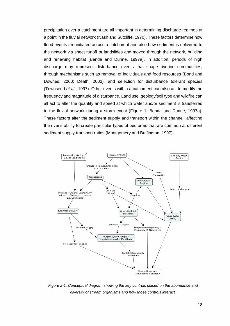
Climate plays a central role in the formation of physical habitat, acting both within the

channel and at catchment-wide scales and above (Figure 2-1). Precipitation drives

physical habitat creation and renewal as it creates the floods which shape river

channels (Benda et al., 2004). The intensity, frequency and total amount of

18

precipitation over a catchment are all important in determining discharge regimes at

a point in the fluvial network (Nash and Sutcliffe, 1970). These factors determine how

flood events are initiated across a catchment and also how sediment is delivered to

the network via sheet runoff or landslides and moved through the network, building

and renewing habitat (Benda and Dunne, 1997a). In addition, periods of high

discharge may represent disturbance events that shape riverine communities,

through mechanisms such as removal of individuals and food resources (Bond and

Downes, 2000; Death, 2002), and selection for disturbance tolerant species

(Townsend et al., 1997). Other events within a catchment can also act to modify the

frequency and magnitude of disturbance. Land use, geology/soil type and wildfire can

all act to alter the quantity and speed at which water and/or sediment is transferred

to the fluvial network during a storm event (Figure 1; Benda and Dunne, 1997a).

These factors alter the sediment supply and transport within the channel, affecting

the river’s ability to create particular types of bedforms that are common at different

sediment supply-transport ratios (Montgomery and Buffington, 1997).

Figure 2-1: Conceptual diagram showing the key controls placed on the abundance and

diversity of stream organisms and how those controls interact.

19

At the broadest scales, temperature plays a role in controlling the distribution of

vegetation, potentially altering flood hydrographs (Beven et al., 1984) and runoff

erosion rates (Douglas, 1967), and in limiting the rate of weathering and therefore

sediment supply to the stream network (Walker et al., 1981). Water temperature has

a limited effect on physical habitat but it is closely linked with air temperature in almost

all streams (Webb et al., 2003), with only those supplied solely from groundwater

sources having weaker relationships to ambient air temperatures. It is also controlled

by the amount of channel shading by vegetation, which again is ultimately a result of

climate controlled vegetation patterns (Stott and Marks, 2000).

Humans have an ever increasing impact on physical habitat, with densely populated,

developed nations, such as the UK, particularly affected. Channels are directly

impacted by extensive modifications (e.g. >40% by length directly modified in the UK;

Seager et al. 2010), largely for flood control or impoundment, whilst changes in

catchment land use (e.g. urbanisation, deforestation or intensive agriculture) alter the

runoff of water, sediment and pollutants (Coe et al., 2009).

Geomorphological classifications of physical habitat first began to make the link

between processes and observed habitat types, with the seminal study of

Montgomery and Buffington (1997) creating a classification of mountain stream

morphologies based on reductions in slope and a change from supply to transport

limited morphologies. Montgomery et al. (1999) linked these channel classifications

to the distribution and abundance of salmonid spawning, hypothesising that channel

type, based on bed slope, limits available spawning area. This early work was further

supplemented by Benda et al. (2004) who showed that the interaction between river

networks and catchment disturbances imposes a spatial and temporal pattern on river

habitat distribution, namely via tributary effects whereby large volumes of sediment,

delivered by hillslope-connected tributary channels, create changes in channel slope

and morphology at junctions with high order trunk channels. Their work also showed

that drainage density plays an important role in the routing of sediment through a

channel network. Higher drainage densities create a greater proportion of high order

channels that are likely to be uncoupled from hillslope processes and are typically

transport limited, similar to many catchments in the UK. Wohl (2005) explored the

relationship between reach scale morphology and physical controls across a large

dataset finding that channel slope, width and sediment size are the key controls

placed on reach scale morphology at large spatial scales. Wohl and Merritt (2008)

again used a large dataset of mountain streams to understand the differences

20

between the channel types first proposed by Montgomery and Buffington (1997). The

patterns between step-pool, pool-riffle and plane-bed channels indicated that physical

form is adjusted to maximise flow resistance and reduce downstream variability in

flow resistance. These classifications form the basis for linking organisms and

habitats.

Different approaches for linking physical habitat and

species’ distributions

Researchers from both stream ecology and fluvial geomorphology have investigated

the relationships between organisms and physical habitat, yet few have incorporated

the other’s discipline into their work, leading to limited success. There is a long history

of attempts to quantify the habitat preferences of organisms residing in the channel

bed, with some of the earliest being by Percival and Whitehead (1929) who quantified

organism richness in different channel beds in Yorkshire. Hundreds of subsequent

studies have looked at the local influence of substrate composition, channel gradient

or flow velocity on stream organisms (e.g. Riley, 1921; Brusven and Prather, 1974;

Reice, 1980; Hawkins et al., 1982; Lammert and Allan, 1999). Some of these have

described physical habitat in great detail, such as Beauger et al. (2006) who studied

the relationship between velocity, depth, substrate and macroinvertebrate community

structure and Lancaster and Hildrew (1993) who investigated the micro-distribution of

benthic macroinvertebrates in relation to flow refugia.

In contrast to detailed studies of individual taxon habitat requirements, Vannote et al

(1980) took a larger scale view of these relationships by proposing the river continuum

concept (RCC) which speculated that the distribution and abundance of stream

organisms changed downstream in an orderly sequence based upon increasing

discharge and subsequent morphological changes. This was one of the first attempts

to produce a general, conceptual model linking physical process, habitat and

organisms, and produced testable predictions. The RCC also stimulated several

subsequent models. Frissell et al. (1986) proposed that river habitats were organised

in a hierarchy based on the spatial and temporal arrangement of physical network

features and the pool of species available. Montgomery (1999) proposed the notion

of process domains, regions within river networks where similar geomorphic

processes produced similar physical habitat, rather than the simple trends in habitat

envisaged by the RCC. These have been joined by others (e.g. Benda et al., 2004;

21

Thorp et al., 2006): what unites them is an attempt to develop a conceptual framework

in which mechanistic links between geomorphology and ecology can be made.

Many of the conceptual models that have been developed highlight the important role

played by disturbance in determining riverine biodiversity. Disturbance regimes (e.g.

floods, landslides, fires) are seen as being important in delivering sediment and

woody debris to low order channels, which in turn help to form the physical habitats

used by organisms (Benda et al., 1997a; 1997b). There is a general consensus that

the dynamic interplay between sediment calibre, supply and transport, which controls

the distribution of bedforms and the disturbance regime, is the key driver of spatial

and temporal physical habitat patches (Poff and Ward, 1990; Townsend and Hildrew,

1994; Wu and Loucks, 1995). Disturbance in an ecological sense refers to events that

remove organisms and free up resources such as space, and have long been

considered an important factor structuring communities (e.g. Connell, 1978;

Townsend and Hildrew, 1994; Miller et al., 2010). From the perspective of physical

habitat, a disturbance is an event which mobilises sediment within the channel,

leading to the building and renewal of bedforms, such as bars, riffles or pools (Poff

and Ward, 1990; Benda and Dunne, 1997b). The two definitions may have different

thresholds at which an event is termed a disturbance but both require the detachment

and movement of either organisms or sediment from the channel bed, a requirement

that can be assumed to occur at given shear stress thresholds of incipient motion of

the channel bed (Schwendel et al., 2010a).

Alongside disturbance, a second common theme is the importance of scale in

understanding organism-habitat relationships (Vannote et al., 1980; Frissell et al.,

1986; Poff et al., 1997) and this includes combining measurements of physical

features and stream organisms in a channel. Interactions range from a single particle

or organism in the riverbed to distributions across multiple catchments (Frissell et al.,

1986). Selecting the relevant scale when studying the relationship between physical

features and biota is dependent on the intended use of such a study and the features

in question (Wiens, 1989). When looking at the preferred habitat of benthic organisms

it is likely that physical features at a patch scale and smaller would be most relevant

to the study, whereas the study of community level distributions or organisms with a

higher mobility (e.g. fish) is more likely to be conducted at a reach scale or greater in

order to capture enough morphological variability. As most restoration and

management efforts seek to improve the diversity of physical habitat at a reach scale

(>100m) a wider appreciation of community level interaction with physical habitat is

22

required if valid predictions of improvements to the biodiversity of a reach are also to

be made.

Many studies linking organisms such as macroinvertebrates or fish to physical habitat

focus on the ‘patch’ scale. Padmore (1998) introduced the term ‘physical biotopes’ to

describe reaches with a given flow type, as derived from substrate and hydraulic

parameters, thereby providing an explicit link between physical process and habitat

at an ecologically relevant scale. Kemp et al. (2000) furthered this idea by linking flow

biotopes (hydraulically defined) and ‘functional habitats’ (biologically defined) using

the Froude number. Velocity and depth, the main components of the Froude number,

were proven to be the main differentiators between biotopes with a clear division

between fine and coarse bedded streams and their associated macrophytes. Newson

and Newson (2000) discussed the link between physical biotopes and

macroinvertebrates using flow type and how both ecologists and geomorphologists

work at similar scales within hierarchical systems that are not yet linked. Subsequent

work has shown that distinct assemblages of organisms are found in different

biotopes (e.g. Armitage and Cannan, 2000; Dallas, 2007; Demars et al. 2012).

Biotopes provide a better definition than patch or reach as they have a better

conceptual underpinning when linking process and habitat.

Ecologists have also been considering habitat-organism interactions at scales similar

to biotopes. Statzner et al. (1988) speculated that by understanding the conditions

near the river bed, given by measures such as Froude number, Reynolds number

and shear velocity, which reflect the initiation of sediment transport that renew and

build physical habitat, it should be possible to predict the macroinvertebrates that are

likely to be present. Subsequent small-scale observational studies have provided

evidence to support this by linking trait categories to local flow hydraulics (Lamouroux

et al., 2004; Tomanova and Usseglio-Polatera, 2007). Demars et al. (2012) found that

Froude numbers correlated well with expected trait assemblages in several UK rivers

and biotope type explained 40% of the variability seen in trait distributions.

Experimental evidence has also supported this, such as McCabe and Gotelli (2000)

who discovered that species abundance was lower but richness was higher in an

experimentally disturbed stream, whilst Effenberger et al. (2008) demonstrated

different local macroinvertebrate community compositions between disturbed and

undisturbed areas. These studies show the potential for understanding how the

habitat preferences of organisms relate to sediment transport and supply and is

clearly key to developing knowledge of how macroinvertebrate communities interact

23

with their physical environment and its disturbance regime. Pedersen and Friberg

(2007) found substantial variations in invertebrate abundance between riffles judged

to be of the same unit, as further investigation revealed physical differences in riffle

consolidation and substratum heterogeneity. These findings question whether a

morphological unit, for example a pool-riffle sequence, provides a valid scale when

assessing invertebrate communities as significant local scale variation exists.

Nevertheless, this shift towards more general models of habitat structure/formation,

which minimise the reliance on simplified classifications of habitat units and which are

based in well-understood process-based theory are likely to provide a better

understanding of the links between geomorphology and ecology, and one that should

be more reliable to predicting the effects of environment change (Vaughan et al.,

2009; Urban et al., 2016).

The role of species traits

An important development in deciphering the links between physical habitat and

macroinvertebrate communities has been the widespread adoption of species’

ecological traits alongside traditional, taxonomic descriptors of communities such as

species richness or abundance (Townsend et al., 1997; Lamouroux et al., 2004;

Bonada et al. 2007). The use of traits, such as reproduction method, lifespan, size,

mobility and dispersal, make ecological links more explicit and also allow an

evolutionary perspective. Southwood (1977, 1988) was the first to introduce the idea

that physical processes acting at a large spatial scale create a template of habitat

patches within which organisms evolve life history strategies. Further studies

developed this idea in rivers by adding scales of spatial and temporal variability driven

by habitat heterogeneity (Townsend, 1989; Poff and Ward, 1990) and frequency of

disturbance (Townsend and Hildrew, 1994). Townsend and Hildrew (1994) provided

a conceptual model of how species traits may relate to physical habitat by plotting the

distribution of traits on axes of: i) habitat heterogeneity, indicating the provision of

refugia from disturbance, for which biotope diversity can be used as a proxy, and ii)

disturbance frequency (Figure 2-2). It was proposed that low habitat heterogeneity

and frequent disturbance would select for species displaying traits required to survive

in disturbed system and the resultant physical habitat itself (e.g. short lifespans, fast

reproductive cycles; Figure 2-2). Field validation of these predictions has been

provided by a range of studies. Bonada et al. (2007) found evidence for species with

particular traits existing in intermittent and ephemeral (frequently disturbed)

24

Mediterranean streams, whilst species traits became less closely coupled to physical

habitat features in less frequently disturbed systems with a greater provision of

refugia. Townsend et al. (1997) found that riverbeds disturbed more frequently by

high flows contained a higher percentage of taxa with traits indicative of resistance

across a dataset of 54 streams in New Zealand, whilst Lamouroux et al. (2004) found

that invertebrate traits including size and body form were correlated with hydraulics

in 38 river reaches in France.

Figure 2-2: Reproduced from Townsend and Hildrew (1994). Conceptual diagram of the

relationship between species traits and spatial heterogeneity, the provision of refugia and

temporal heterogeneity, the disturbance frequency. The table shows the expected range

of traits present at either Area A or B.

25

The relationship between species traits and environmental conditions has been

shown to be complex as species possess multiple traits that can be impacted in

different ways by disturbance, making species relations to single environmental

gradients often appear decoupled when in reality there is a relation (Poff et al., 2006).

They also showed that many traits are readily adaptable to deal with disturbance (e.g.

size at maturity), further complicating their application (Poff et al., 2006). A need for

a framework that considers multiple traits along with multiple environmental gradients

has been discussed by both Poff et al. (2006) and Verberk et al. (2013) but progress

has been slow due to the complexity of trait-environment interactions. For example,

Lamouroux et al. (2004) found that macroinvertebrate traits including body size,

attachment mechanism, feeding habits, lifespan and reproduction/dissemination

strategy all significantly correlated with physical habitat variables in two catchments

in France. Similarly, anthropogenic modification of the river environment can affect

many traits simultaneously (e.g. through impacts of fine sediments; Larsen and

Ormerod, 2010). Mouillot et al. (2013) developed a generic framework for relating

traits to disturbance, by proposing an approach that identifies both winner and loser

species due to disturbance. Trait approaches have shown large potential, are clearly

linked to biological processes and are benefitting from recent conceptual

developments (e.g. Mouillot et al., 2013) but there is still more that can be explored.

Methods for predicting bedform distribution and bed

disturbance

Traditional ecological models are static and correlative, making them poor at

extrapolating beyond the conditions under which they were calibrated (Urban et al.,

2016). As changing conditions (e.g. climate, land use) are a key component of current

and future interactions between physical habitat and ecological function, process-

based models that capture these changes are needed (Vaughan et al., 2009). To

address the specific aims of this thesis, a process-based approach that captures the

key controls on sediment transport and physical habitat distribution in alluvial rivers

is required. These controls, primarily the flow conditions of the river and the nature

(i.e. size and shape) of the river sediment (Shields, 1936; Andrews, 1983; Parker,

1990), are captured by various approaches that are capable of determining the onset

of sediment transport (Figure 2-3). An approach is needed that can be applied at a

national scale and is compatible with existing datasets, which are typically limited in

their information of channel morphology, sediment and flow (Figure 2-3). In the

26

absence of reliable measurements of the processes governing bedform distribution

and disturbance, a simple means of estimating sediment transport is needed.

Sediment transport equations provide a well-understood, detailed method for

studying the onset of riverbed disturbance but require detailed information on flow

velocities and/or sediment composition and as such, can only be applied at scales

where the data can be obtained within time and cost constraints: this typically limits

them to reach scales or less (Ackers and White, 1973; Yang, 1976; Mueller et al.,

2005). Although these mechanistic approaches could provide new insights into

geomorphology-ecology interactions, they are far too complex to be applied generally

at a national scale.

Stream power has been widely used at catchment or regional scales to predict zones

of erosion and deposition (e.g. Newson et al., 1998a; Knighton, 1999; Parker et al.,

2011; Bizzi and Lerner, 2012) and channel features (e.g. Gurnell et al, 2010; Vaughan

et al., 2013). It has modest data requirements and provides a simple means of

estimating the energy available to do work in the channel, based on channel slope,

discharge and, when calculated per unit area (termed specific stream power), channel

width (Bagnold, 1977). It has grown in popularity as the spatial scale of studies has

increased with the advent and now wide use of Digital Terrain Models (DTM’s) for

catchment studies (Knighton, 1999; Bizzi and Lerner, 2012; Phillips and Desloges,

2013). Whilst stream power provides a rapid, simple means of estimating sediment

transport capacity it does not include any measurement of the sediment being

transported through a reach and as such cannot reliably predict sediment transport

rates. Parker (2011) attempted to improve the physical basis for using stream power

by calculating dimensionless critical stream power, based on Einstein’s (1950)

dimensionless sediment transport equation, finding that it corresponded well with

sediment transport rates measured in laboratory flumes and empirical evidence that

predicted critical unit stream power to be proportional to Di1.5 (Di = size of mobilised

particles in mm; Petit et al., 2005). The inclusion of a measure of bed grain size in

the dimensionless critical stream power equation provides a simple means of

estimating whether the material making up the channel bed is in motion at the given

stream power, essential in predicting sediment transport.

Another potential method of assessing the sediment transport capacity of a river

reach is by using the Shields Regime Diagram (Shields, 1936). The diagram

estimates the mode of sediment transport experienced by a channel bed based on

27

flume studies of particle motion and suspension. Two axes are combined to provide

this information. The first axis is the particle Reynolds number, which is effectively a

measure of the mean sediment size of the riverbed. The second axis is dimensionless

shear stress, a measure of the propensity for movement of sediment on the riverbed,

which is calculated using flow depth, channel gradient and mean sediment size

(Shields, 1936). Together, these axes differentiate between different geomorphic

processes occurring at each location, chiefly bed-load and suspended-load transport,

and the range of substrate sizes present in the riverbed, which in combination have

been shown to control alluvial bedforms (van Rijn, 1984; Buffington and Montgomery,

1997).

The Rouse number, the ratio of settling and shear velocities, provides an alternative

means of finding the mode of bed material transport at a site. Dade and Friend (1998)

introduced the terms competence and capacity to show that channels exhibit different

sediment transport modes based on sediment supply-transport ratios. Competence

is a measure of the largest grain size the can be mobilised by a flow, whilst capacity

is a measure of the sediment capacity of a stream that is not limited by sediment

supply. They showed that abrupt changes in the downstream fining of bed substrate

represented the point at which channels switched transport modes, based on the

Rouse number. The Rouse number is not used in the thesis as it has many similarities

to the thresholds of bed and suspended load transport used in the Shields diagram,

the chosen method for quantifying the mode of transport and disturbance in Chapter

4.

These different approaches are used at varying times in the following chapters largely

depending on their data requirements in relation to the available datasets. Chapter 3

uses specific stream power to predict the distribution of bedforms across the UK.

Specific stream power was chosen due to its low data requirements and previous

performance in predicting channel features (Vaughan et al., 2013). Chapter 4 uses

the Shields regime diagram to link invertebrate community diversity and function to

the distribution of physical habitats and disturbance. The Shields diagram was

selected due to its well-defined association with physical process (i.e. bed load and

suspended load transport) and its relative simplicity in comparison to more rigorous

methods for estimating sediment transport. Chapter 5 uses critical specific stream

power to estimate when disturbance occurs across time-series flow data from gauging

stations. It was selected again due to its low data requirements and its proven

relationship to gravel-bed rivers, which are common across the UK. Chapter 6

28

compares the use of these methods in the previous chapters and discusses their

potential applications in river management.

Figure 2-3: A conceptual diagram of the progression of development of a simple method

for predicting the frequency of disturbance at a location. Explanatory power, in terms of

process, is increased with the addition of the mode of sediment transport. The simple

variables required for each method are included.

Climate change and the need for better prediction

The evidence for future climate change is now unequivocal and much of the debate

around the river environment is centred on whether we are already beginning to be

impacted by climatic changes and what future predictions can be made (Coulthard et

29

al., 2012; Kendon et al., 2014; Markovic et al., 2014). Predictions of climate change

impacts on the UK have been refined over the past two decades and now provide

detailed information about the total amount, frequency and intensity of precipitation

events (e.g. Murphy et al., 2009), which in turn will affect the hydrological cycle,

sediment transport and disturbance regimes in the fluvial network. Despite these

advances, there is still uncertainty about the impacts on the flow regime. In many

temperate regions of the world, there has been a general assumption that flood

frequency and magnitude will increase, but current evidence suggests that only flood

frequency and timing are changing, whilst magnitude remains the same (Mallakpour

and Villarini, 2015; Bloschl et al., 2017; Wasko and Sharma, 2017).

Across the catchment and over longer timescales, the delivery of sediment to the

channel is likely to increase as more frequent and severe storms are predicted to

trigger more landslides and increase sheet runoff (Wilby et al., 1997), a principal

delivery mechanism of fine sediment to the channel. Land cover changes, which in

turn may be a response to changing climate, could act to exacerbate this increase

(Coulthard et al., 2012). Much of this relates to intensive farming practices, which

increase soil compaction and remove natural vegetation that can store water and

retain fine sediment (i.e. topsoil), thereby increasing sheet runoff (Evans et al., 2016).

A continued growth of urban areas, with extensive impermeable surfaces, would also

accelerate runoff. The increasing delivery of fine sediments is recognised as a major

stressor on riverine communities (e.g. Wood and Armitage, 1997; Larsen and

Ormerod, 2010; Kemp et al., 2011; Jones et al, 2014).

These changes in streamflow and sediment supply are likely to lead to morphological

changes in channels over coming decades. Both short and long term changes are

likely as the shape, gradient and sediment composition of channels respond to new

environmental conditions. A better understanding of the relationship between these

hydromorphological changes and community composition and function is key to

making future predictions of climate impacts on freshwater communities. Critically,

the novel conditions generated by climate and land use changes are likely to

challenge traditional approaches to predictive modelling, especially when the impacts

of different stressors may interact (Piggott et al., 2015). Despite these challenges,

prediction will be as least as, if not more, important than it has been in the past. To

address the shortfall of traditional predictive models, reliable, accurate, process-

based models of river channels and organism distributions and function are needed

(Urban et al., 2016; subsequent chapters of this thesis).

30

Nationwide datasets and the emergence of river

restoration in the UK

The greater availability of remotely sensed imagery and increased computing power

has driven the collection of physical variables across larger spatial scales over the

last decade (Carbonneau et al., 2012). This move to a catchment scale approach to

environmental management across Europe has largely been driven by the Water

Framework Directive (2000/60/EC). The Directive places emphasis not just on

improving the ecological and water quality of freshwater systems but also on

achieving ‘good hydromorphological status’. Improvements in water quality over

recent decades have highlighted the impact of physical modification on the

hydromorphology of freshwater systems (Vaughan et al., 2009). A slew of new

restoration techniques have followed, focussing on restoring river reaches to a

‘natural’ state often by techniques such as meander reintroduction, installation of

large woody debris (LWD) or by flow barrier removal (Newson and Large, 2006). To

fully assess whether these new approaches are appropriate for a river reach there is

an urgent requirement for tools that place a reach within its larger catchment setting

with regards to habitat type and sediment supply and transport (Everard, 2004). This

effort has led to a number of papers attempting to classify channel and habitat types

based mostly on rapid GIS-derived variables and then linking the classification with

ecological impacts. For example, May and Lisle (2012) used a digital elevation model

to assess the availability of salmonid habitat, based on channel slope classifications,

across multiple catchments in the Pacific Northwest. Richards et al. (1997) found that

GIS-derived reach scale variables (e.g. cross-sectional area, percentage of fines)

were strongly correlated with invertebrate life-history traits, whilst catchment scale

variables (e.g. geology) were less well correlated, whilst Bizzi et al. (2016) used

various remote sensing techniques to characterise the hydromorphological properties

of river across Europe.

The development of catchment scale tools requires large, often nationwide, datasets

to understand the range of channel types and physical habitats that are present. Many

studies focus on local scale classifications and often overlook their context within a

catchment system (Everard, 2004), especially when considering their role in sediment

supply and transport. The UK may be unique in having a collection of large scale

databases of river attributes that has been ongoing since the 1990s (Vaughan and

Ormerod, 2010). In addition to routine water quality and biological (primarily

31

macroinvertebrate) sampling, the Environment Agency’s River Habitat Survey (RHS)

database has assembled >24,000 sites spanning a period since 1994. RHS is a

simple tool to quickly characterise the physical structure of rivers as a series of 500m

survey reaches, with information recorded for the dominant bed/bank materials, flow

types, instream and riparian vegetation and simple morphological attributes such as

presence/absence of bedform features, bank profiles and any artificial features or

modifications to the channel (Raven et al., 1997; Environment Agency, 2003). Many

studies have utilised the RHS database since its creation (e.g. Jeffers, 1998; Hastie

et al, 2003; Orr et al., 2008; Bizzi and Lerner, 2012) and the UK-wide coverage of its

two national baseline surveys (1994–6 and 2006–8; Seager et al., 2010) have greatly

increased its potential usefulness when used alongside GIS-derived variables.

RHS has supported efforts in the UK, and other parts of Europe, to improve the

understanding of the links between physical channel processes and biotopes

(Newson et al., 1998b). Jeffers (1998) ordinated the first RHS baseline based on the

map-derived variables of altitude, slope, distance from source and height from source,

finding that physical habitat features could be predicted using only these variables.

Vaughan et al. (2013) built on this approach, adding a number of GIS-derived

variables to the method, improving the predictive capability of the ordination. It was

found that a combination of specific stream power and catchment area were robust

predictors of the physical attributes of channels. Another approach is to look at

species specific distributions across Britain in relation to physical habitat features from

the RHS database, as has been completed for organisms including bats (Langton et

al., 2010), river birds (Vaughan et al., 2007) and macro-invertebrates (Naura and

Robinson, 1998; Hastie et al., 2003; Vaughan and Ormerod, 2012). Other studies

have taken parts of the RHS database in an attempt to either classify channels based

on flow biotopes (Harvey et al., 2008a), stream order (Orr et al., 2008), stream power

(Bizzi and Lerner, 2012; Vaughan et al., 2013) or sediment transport regimes (Parker

et al., 2012). RHS has also been used to study the links between physical channel

attributes and rock type (Harvey et al., 2008b), pool-riffle spacing (Emery et al., 2007)

and aquatic plant morphotypes (Gurnell et al., 2010). Bizzi and Lerner (2012) utilised

GIS-derived controls such as channel slope, specific stream power and floodplain

extent along with data describing the physical habitat types, from the RHS database,

to identify typologies of channel along the River Lune in north England. This wide

range of studies demonstrates the value of large scale hydromorphological datasets,

such as RHS, particularly for planning targeted efforts at a catchment or national

scale.

32

Conclusions

Habitat-organism interactions in rivers are governed at the largest scales by climate,

geology and, increasingly, human actions. These broad controls are imparted on

rivers via trends in water chemistry, flow regime and sediment supply/transport, which

in turn determine the conditions that are tolerated by organisms which specific suites

of traits. Studies of the habitat preferences of freshwater organisms have a long

history (Percival and Whitehead, 1929) but have remained restricted to either to small

scales (i.e. several organisms within a river reach) or to conceptual studies of larger

scale trends (Vannote et al., 1980; Townsend and Hildrew, 1994), largely due to data

collection constraints. The advent of open datasets and rapid data collection methods

(e.g. LiDAR) now provides greater opportunities for the large scale collection of

geomorphic data (Carbonneau et al., 2012). Traditional ecological studies of habitat-

organism interactions use static, correlative models that are considered to be poor at

extrapolating to environmental change (e.g. in climate or land use). As robust

predictions of these changes continue to gain importance, models grounded in

process-based theory, which minimise the reliance of simplified classification of

habitat units may offer a better approach (Urban et al., 2016).

In recent years, widespread efforts have taken place across freshwater sciences to

promote studies with a multidisciplinary, holistic approach (Vaughan et al., 2009). A

push from legislation (e.g. the WFD) has seen river management, particularly across

the UK and continental Europe, transition to a catchment based approach (delivered

via River Basin Management Plans). Despite this, the understanding and tools

required by river managers to robustly plan interventions at this scale are lacking and

efforts to combine the traditionally separate disciplines of hydrology, geomorphology

and ecology are urgently needed (Vaughan et al., 2009). This thesis aims to be part

of those efforts by contributing to our understanding of geomorphology-ecology

interactions, with particular focus given to the role of bedform distribution and

disturbance in structuring ecological communities.

The UK is uniquely positioned to address these research gaps as it has possibly the

densest, longest-term record of flow, chemistry and biology monitoring in the world.

These often undervalued datasets enable studies of geomorphological-ecological

interactions across large spatial scales and relatively long timespans (>10 years).

Here, I make use of different collections of five of these datasets as the basis of each

analytical chapter.

33

3 Controls on the spatial distribution of bars within

the alluvial rivers of Great Britain

Abstract

Bars function as important in-river sediment stores that can significantly alter channel

form as well as acting as unique transitional habitats that alternate between terrestrial

and fluvial realms. Despite considerable effort to explain the controls on bar formation

at local reach scales, our understanding of such controls at network and regional

scales has been limited until recently by the paucity of catchment-scale observations.

Such lack of understanding could limit the effectiveness of river restoration strategies

that are increasingly being implemented in catchments across Europe. This chapter

utilized 1480 River Habitat Survey sites across Great Britain to model the spatial

distribution of bars, using specific stream power at bankfull discharge (ω), coupled

with mean riverbed grain size, to reflect the balance between river energy and relative

riverbed mobility. Bars were most commonly found in gravel-bed rivers where ω > 30

W m-2 at bankfull discharge, conditions typical of upland rivers found in northern and

western Britain. Bar prevalence was overestimated in channelized rivers, likely due

to increased flow velocities inhibiting the development of depositional bedforms or the

removal of coarse material for flood control/navigation, and in chalk geologies, likely

due to their uniquely dampened flow regimes. Prevalence was underestimated in

small, lowland rivers with cohesive riverbeds and abundant channel vegetation. My

data helps to identify key elements in river and catchment management that must be

addressed if bars are to be restored and maintained in British rivers.

34

Introduction

Bars are a basic morphological unit of alluvial channels, forming part of the ubiquitous

riffle-bar-pool sequence that provides regularity to the channel planform, most

obviously in rivers with alternating bars, meander bends or braids (Leopold and

Wolman, 1957; Kleinhans, 2010). They are key in-channel sediment storage features

(Benda and Dunne, 1997), play an important role in channel dynamics by dictating

the pattern of bank erosion and channel planform evolution (Kleinhans, 2010), and

also create unique habitats for a range of organisms including birds, invertebrates

and macrophytes (Eyre et al., 2001; Madsen et al., 2001). Our current understanding

of the controls on the spatial distribution of bars is largely split between theoretical

knowledge of the processes that build and sustain bars (e.g. river planform, sediment

transport and supply) and applied knowledge of where human-induced changes in

flow and sediment regimes (e.g. via channelization) has led to the demise of bar

forms. Here, we aim to discover the major controls on the spatial distribution of bars,

at a scale relevant to river management, by comparing predictions of bar occurrence

from a statistical model based on river process with real-world observations of bar

occurrence in often heavily-managed river systems.

Bars are commonly classified into point, alternate and mid-channel according to

differences in their mechanisms of formation and position within the channel. They

can be split into ‘free’ and ‘forced’ depending on their ability to migrate downstream

(Seminara and Tubino, 1989; Kleinhans, 2010). Free bars form in a straight channel

due to the instability of turbulent flow creating perturbations (bars) in the erodible

channel bed (Tubino et al., 1999). Both alternate and mid-channel bars can form in

this way when a threshold width-to-depth ratio is exceeded (Kleinhans, 2010),

although the latter also requires a high relative sediment supply (Hooke, 1986;

Kleinhans and van den Berg, 2011). Mid-channel bars often form where abrupt

increases in channel width and sediment supply occur, such as at confluences or

where rivers exit mountain ranges (Leopold and Wolman, 1957; Ashmore, 1982,

1991; Ashworth, 1996). High flow events can also rapidly increase channel width in

portions of the river network, promoting bed-material deposition and mid-channel bar

building (Hooke, 1986; Carson and Griffiths, 1987; Friedman et al., 1996; Madej and

Ozaki, 1996). Forced (or fixed) bars are formed by either (1) variations in local

channel width, such as around fixed obstructions (e.g., a large boulder/fallen tree) or

at confluences (Kleinhans, 2010) or (2) in meander bends where channel curvature

forces the flow to deposit material on the inside of the bend. Point bars, which are

35

formed when secondary flow currents stack bed-material up on the inside of a

meander (Nanson, 1980; Dietrich and Smith, 1983), are the most common example

of forced bars.

The mechanism of transition from a channel with free alternate bars to forced point

bars is widely debated. Bar theory suggests that free bars promote bank erosion,

increasing channel curvature until the bars become fixed, whilst bend theory suggests

that fixed bars are induced by channel curvature (Blondeaux and Seminara, 1985;

Tubino and Seminara, 1990; Tubino et al., 1999). Seminara and Tubino (1989)

showed that in a straight river, alternate bars migrate fast enough to uniformly erode

the banks, widening the channel and eventually forming mid-channel bars, which

suggests that another factor, such as bank erodibility, controls a change from a

straight to meandering channel. Vegetation or cohesive sediment may act to

decrease bank erodibility, with straight channels that have stronger banks typically

becoming narrower and deeper (Hey and Thorne, 1986; Soar and Thorne, 2001),

potentially promoting localized bank erosion that leads to meandering. Channels with

weaker banks become wider and shallower, developing a braided planform (Parker,

1976; Xu, 2002).

Advances in our understanding of the controls on bed-material routing through the

river network and of the processes underlying bar formation have been made through

field (Lewin, 1976; Nanson, 1980; Hooke, 1986; Church and Rice, 2009), numerical

modelling (Lisle et al., 2000) and laboratory–based (Ashmore, 1991; Lisle et al., 1991)

studies. Despite these advances, relatively little attention has been given to bar

distribution at the network-scale with most studies instead focusing at the reach scale,

largely due to data constraints as network-scale analysis is too large for any field

campaign and beyond current remote sensing capability (Legleiter et al., 2004;

Carbonneau et al., 2012). However, river management in much of Europe is now

planned at the catchment scale and an understanding of the distribution of bars at a

similar scale is needed by river managers in order to: (1) target restoration efforts at

river reaches where bar restoration would be sustainable; (2) monitor parts of the

network where significant accretions of sediment are expected, as these may

increase flood risk (Lane et al., 2007); and (3) mitigate and plan for future changes in

river morphology (e.g. due to climate or land use change) that may reduce bar habitat,

impacting upon freshwater organisms and the key ecosystem services they provide

(Macklin and Lewin, 2003; Coulthard et al., 2012).

36

In this study, we aim to quantify the conditions under which point, alternate, and mid-

channel bars develop in rivers across Great Britain to gain insight of the controls on

bedform habitat features at the scales at which river management is now planned.

The presence of different bar types was obtained from 1480 semi-natural and

modified rivers with River Habitat Survey (RHS), the standard method for recording

river physical habitat in England and Wales (Seager et al., 2012). We developed a

statistical model that couples specific stream power, a measure of a river’s capacity

to perform work on its bed and banks (or modify the channel form through sediment

transport), with mean riverbed grain size to reflect the balance between this energy

and the relative riverbed mobility. Specific stream power has been used widely in

sediment transport studies (Bagnold, 1977; 1980) to assess channel patterns (Chang,

1979; Nanson and Croke, 1992; Van Den Berg, 1995) and to predict channel features,

(Bizzi and Lerner, 2012; Vaughan et al., 2013). We offer an explanation for the

apparent threshold value of specific stream power required for bar occurrence and

assess shortfalls in the model, accounting for the influence of catchment geology,

channelization and emergent vegetation upon bar formation.

Methods

3.3.1 RHS

The RHS was developed in 1994 to characterize the physical character and quality

of river habitats across the UK (Raven et al., 1998). It has since been used at over

25,000 sites in the UK and elsewhere across Europe. An individual RHS involves a

survey of a 500-m length of channel with ten spot-checks that record features at 50-

m intervals and a sweep-up section that records the presence, absence, or

extensiveness (≥33% of channel length) of features within the reach (Raven et al.,

1998). Features include the type and extent of channel vegetation, any modifications

to the channel and the dominant substrate type. Channel dimensions are also

measured on a straight, uniform section, preferably across a riffle, at each survey site

(Raven et al., 1998). Finally, each RHS location has an accompanying estimate of

channel slope, measured from 1:50,000 scale maps over a 1-km length centred on

the mid-point of the study reach (Raven et al., 1998). Map-derived channel slope

corresponds well with field measurements (Montgomery et al., 1998) and is often

more accurate than slope derived from digital elevation models due to errors in

channel length estimation as a result of pixel size (Clarke et al., 2008; Fisher et al.,

2013).

37

Point, alternate (side) and mid-channel bars were identified and recorded separately

in the RHS, with point bars located on the inside of distinct meanders, alternate bars

attached to the bank but not located on the inside of distinct meanders, and mid-

channel bars detached from both riverbanks with elevations below bankfull depth to

distinguish them from mature islands (Raven et al., 1998). Each bar type was further

sub-divided as ‘vegetated’ (>50% cover) or ‘un-vegetated’ (<50% cover). The

presence or absence of six bar types (i.e., three types, each sub-divided between

vegetated and un-vegetated) within each 500-m reach was recorded using the

sweep-up component of RHS. The spot-check component was not used as bars

occurring between each 50-m check would be missed.

This study utilized the most recently available baseline RHS data for Great Britain:

the 2007-08 baseline survey of England and Wales (consisting of 4849 reaches) and

the 1995-96 baseline survey of Scotland (consisting of 769 reaches) (Seager et al.,

2012). Baseline surveys were chosen because they provided systematic coverage by

randomly selecting watercourse reaches in every 10-km grid square, with three

reaches selected per 10-km2 in England and Wales and one reach selected per 10-

km2 in Scotland. The initial sample size was reduced to 1480 survey reaches by

filtering out (1) non-alluvial channels (<80% survey reach composed of alluvial bed

material); (2) sites without measurements of average bed slope or bankfull width and

(3) sites where reliable discharge estimates could not be extracted, typically

topographically flat areas with multiple channels and artificial drainage networks (e.g.

in parts of Eastern England) (Figure 3-1A). Whilst this approach is limited by the

geomorphic information recorded by RHS (Newson, 2002), it is offset by the ability to

carry out large scale assessments of river morphology (e.g. Newson et al., 1998a;

Emery et al., 2004; Harvey et al., 2008).

3.3.2 Discharge Estimation

Previous studies have shown that bankfull discharge, the flow that fills the channel to

the bank-tops, is the most influential discharge on channel form (Pickup and Warner,

1976; Williams, 1978; Andrews, 1980; Phillips and Jerolmack, 2016). Yet its

infrequent nature and the natural variation in channel capacity along a river reach

make it difficult to estimate (Ferguson, 1981). Andrews (1980) estimated bankfull

discharge to have a recurrence interval of 1.18 to 3.26 years whilst Carling (1988)

estimated it as 0.9 years. In the absence of a nearby gauging station, the median

38

annual flood, or the 2-yr recurrence flow, is typically used instead of bankfull

discharge (Wharton, 1995; Gurnell et al., 2010; Bizzi and Lerner, 2012). A

disadvantage of this approach is that channel-forming (or bankfull) discharge may not

be represented well by median annual flood where the river channel has been

enlarged for flood conveyance (Wharton, 1995). This study used estimates of median

annual flood, originally calculated as part of the Flood Estimation Handbook (Kjeldsen

et al., 2008), which were extracted from the Peak River Flows dataset provided by

the Centre for Ecology and Hydrology (CEH).

3.3.3 Substrate Size

Using a similar method to Gurnell et al. (2010), median substrate size (D50) was

estimated by converting the ten spot measures of substrate type, taken every 50-m

in each 500-m RHS reach, into an average phi score based on approximate values

for median particle size of each size class:

𝐷50 = (−8 ∗ 𝐵𝑂 − 7 ∗ 𝐶𝑂 − 3.5 ∗ 𝐺𝑃 + 1.5 ∗ 𝑆𝐴 + 6 ∗ 𝑆𝐼 + 9 ∗ 𝐶𝐿)

(𝐵𝑂 + 𝐶𝑂 + 𝐺𝑃 + 𝑆𝐴 + 𝑆𝐼 + 𝐶𝐿)

Where BO = boulder, CO = cobble, GP = gravel-pebble, SA = sand, SI = silt and CL

= clay.

3.3.4 Specific Stream Power

As a measure of the ability of river flows to perform work on the boundaries of a

channel (i.e., banks and channel bed), the specific stream power (ω; W m-2) provides

a relatively straightforward approach to measuring the propensity for sediment

transport, and is defined as:

𝜔 =𝜌𝑔𝑄𝑆

𝑤

where ρ is equal to the density of water (1000 kg m-3), g is the gravitational constant

(9.81 m s-1), S is equal to average bed slope (m m-1), as included in RHS, and w is

equal to channel width (m), taken as the bankfull width measured at each RHS site.

3.3.5 Statistical Methods

All statistical analyses were performed in R (v 3.3.0; R Development Core Team,

2016). Generalised Additive Models (GAMs) with a logit link and binomial errors were

used to predict the probabilities of occurrence of the different bar types, based on the

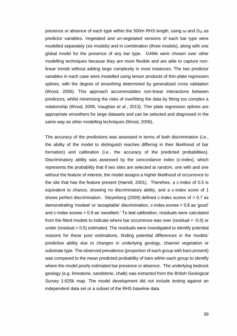
39

presence or absence of each type within the 500m RHS length, using ω and D50 as

predictor variables. Vegetated and un-vegetated versions of each bar type were

modelled separately (six models) and in combination (three models), along with one

global model for the presence of any bar type. GAMs were chosen over other

modelling techniques because they are more flexible and are able to capture non-

linear trends without adding large complexity in most instances. The two predictor

variables in each case were modelled using tensor products of thin-plate regression

splines, with the degree of smoothing determined by generalized cross validation

(Wood, 2006). This approach accommodates non-linear interactions between

predictors, whilst minimizing the risks of overfitting the data by fitting too complex a

relationship (Wood, 2006; Vaughan et al., 2013). Thin plate regression splines are

appropriate smoothers for large datasets and can be selected and diagnosed in the

same way as other modelling techniques (Wood, 2006).

The accuracy of the predictions was assessed in terms of both discrimination (i.e.,

the ability of the model to distinguish reaches differing in their likelihood of bar

formation) and calibration (i.e., the accuracy of the predicted probabilities).

Discriminatory ability was assessed by the concordance index (c-index), which

represents the probability that if two sites are selected at random, one with and one

without the feature of interest, the model assigns a higher likelihood of occurrence to

the site that has the feature present (Harrell, 2001). Therefore, a c-index of 0.5 is

equivalent to chance, showing no discriminatory ability, and a c-index score of 1

shows perfect discrimination. Steyerberg (2009) defined c-index scores of > 0.7 as

demonstrating ‘modest’ or ‘acceptable’ discrimination, c-index scores > 0.8 as ‘good’

and c-index scores > 0.9 as ‘excellent.’ To test calibration, residuals were calculated

from the fitted models to indicate where bar occurrence was over (residual < -0.5) or

under (residual > 0.5) estimated. The residuals were investigated to identify potential

reasons for these poor estimations, finding potential differences in the models’

predictive ability due to changes in underlying geology, channel vegetation or

substrate type. The observed prevalence (proportion of each group with bars present)

was compared to the mean predicted probability of bars within each group to identify

where the model poorly estimated bar presence or absence. The underlying bedrock

geology (e.g. limestone, sandstone, chalk) was extracted from the British Geological

Survey 1:625k map. The model development did not include testing against an

independent data set or a subset of the RHS baseline data.

40

Results & Discussion

Rivers were included from across Britain with very few gaps in their geographic

distribution, with an absence of sites limited to low-lying regions of Eastern England

and the Somerset Levels (Figure 3-1A). RHS reaches ranged in catchment area from

five to 4984 km2, with median annual discharges from 0.1 to 963.5 m3 s-1 and

estimated specific stream powers of between one and 1116 W m-2. The dominance

of coarse gravel-bed rivers in Britain was evident with mean bed material ranging

from silt and clay (9% of sites), through sand (16%), gravel-pebble (46%), and cobble-

boulder (29%) (Figure 3-1B).

Figure 3-1: Distribution of the 1480 RHS sites used in the study on (A) a map of Britain

and (B) the D50-ω axes. The grey, dashed line is a convex hull that incorporates all RHS

sites.

3.4.1 National controls on bar distribution

Point, alternate and mid-channel bars were all most commonly observed in gravel-

bedded rivers with ω > 30 W m-2 that drained areas of northern and western Britain,

including much of Scotland, Wales and north-west and south-west England (Figure

3-2A; Figure 3-3A; Figure 3-4). This change in river type across Britain is often

described as the divide between upland and lowland Britain and is sometimes

denoted as a line between the rivers Tees and Exe (Ferguson, 1981; Figure 3-1A).

The variation in overall bar occurrence was largely driven by alternate bars, the most

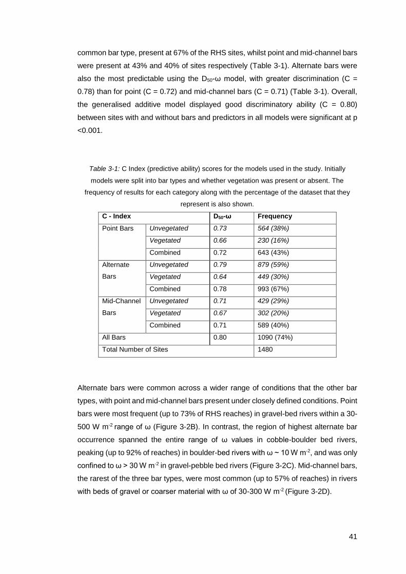
41

common bar type, present at 67% of the RHS sites, whilst point and mid-channel bars

were present at 43% and 40% of sites respectively (Table 3-1). Alternate bars were

also the most predictable using the D50-ω model, with greater discrimination (C =

0.78) than for point (C = 0.72) and mid-channel bars (C = 0.71) (Table 3-1). Overall,

the generalised additive model displayed good discriminatory ability (C = 0.80)

between sites with and without bars and predictors in all models were significant at p

<0.001.

Table 3-1: C Index (predictive ability) scores for the models used in the study. Initially

models were split into bar types and whether vegetation was present or absent. The

frequency of results for each category along with the percentage of the dataset that they

represent is also shown.

C - Index D50-ω Frequency

Point Bars Unvegetated 0.73 564 (38%)

Vegetated 0.66 230 (16%)

Combined 0.72 643 (43%)

Alternate

Bars

Unvegetated 0.79 879 (59%)

Vegetated 0.64 449 (30%)

Combined 0.78 993 (67%)

Mid-Channel

Bars

Unvegetated 0.71 429 (29%)

Vegetated 0.67 302 (20%)

Combined 0.71 589 (40%)

All Bars 0.80 1090 (74%)

Total Number of Sites 1480

Alternate bars were common across a wider range of conditions that the other bar

types, with point and mid-channel bars present under closely defined conditions. Point

bars were most frequent (up to 73% of RHS reaches) in gravel-bed rivers within a 30-

500 W m-2 range of ω (Figure 3-2B). In contrast, the region of highest alternate bar

occurrence spanned the entire range of ω values in cobble-boulder bed rivers,

peaking (up to 92% of reaches) in boulder-bed rivers with ω ~ 10 W m-2, and was only

confined to ω > 30 W m-2 in gravel-pebble bed rivers (Figure 3-2C). Mid-channel bars,

the rarest of the three bar types, were most common (up to 57% of reaches) in rivers

with beds of gravel or coarser material with ω of 30-300 W m-2 (Figure 3-2D).

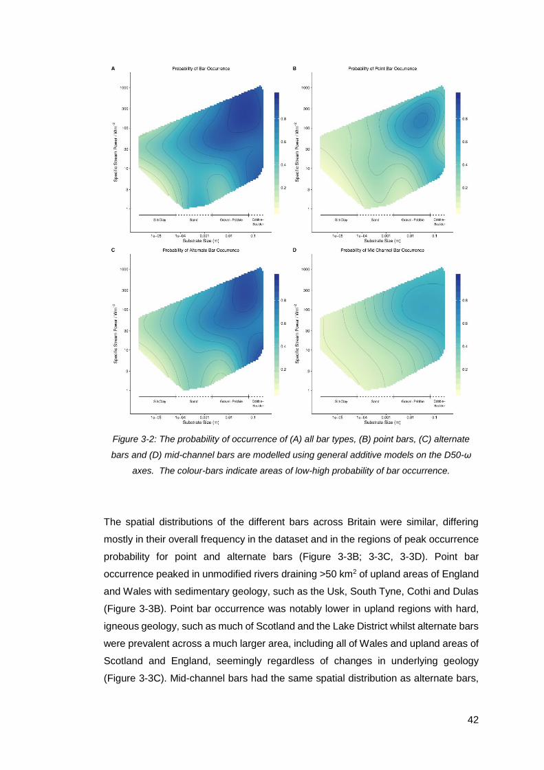
42

Figure 3-2: The probability of occurrence of (A) all bar types, (B) point bars, (C) alternate

bars and (D) mid-channel bars are modelled using general additive models on the D50-ω

axes. The colour-bars indicate areas of low-high probability of bar occurrence.

The spatial distributions of the different bars across Britain were similar, differing

mostly in their overall frequency in the dataset and in the regions of peak occurrence

probability for point and alternate bars (Figure 3-3B; 3-3C, 3-3D). Point bar

occurrence peaked in unmodified rivers draining >50 km2 of upland areas of England

and Wales with sedimentary geology, such as the Usk, South Tyne, Cothi and Dulas

(Figure 3-3B). Point bar occurrence was notably lower in upland regions with hard,

igneous geology, such as much of Scotland and the Lake District whilst alternate bars

were prevalent across a much larger area, including all of Wales and upland areas of

Scotland and England, seemingly regardless of changes in underlying geology

(Figure 3-3C). Mid-channel bars had the same spatial distribution as alternate bars,

43

except their probability of occurrence was lower, reflecting that they were less

commonly found (Figure 3-3D).

Figure 3-3: Interpolated maps of the probability of bar occurrence, as modelled on the

D50- axes, for (A) all bar types, (B) point bars, (C) alternate bars and (D) mid-channel

bars. The colours indicate areas of low-high probability of bar occurrence.

44

At large spatial scales, the type and amount of sediment available to a river, controlled

by geology, climate and human activity, along with a river’s ability to transport that

sediment, controlled primarily by gradient, discharge and width, dictates the planform

of alluvial river channels (Mackin, 1948; Schumm, 1985). River planform is closely

related to the type and abundance of bar forms present within the channel. For

example, point bars are a feature indicative of meandering rivers, whilst mid-channel

bars are common in braided rivers. Crosato and Mosselman (2009) successfully

modelled bar occurrence in a cross-section based on width to depth ratio, bed

roughness, channel gradient and sediment characteristics, all similar components to

the D50-ω model used here.

The relatively modest data requirements to estimate specific stream power have seen

it applied to studies of channel pattern and bar occurrence in rivers globally. Nanson

and Croke (1992) and Ferguson (1981; 1987) reported ranges of ω for meandering

rivers of 10-60 W m-2 and 5-350 W m-2 in Australia and the UK respectively,

corresponding closely to the range of ω with the highest probability of point bar

occurrence in this study (Figure 3-2B). Braided rivers, of which mid-channel bars are

a key feature, are relatively uncommon in Britain but wandering, gravel-bed rivers are

commonly found across upland areas and are likely to accommodate alternate and

occasional mid-channel bars (Newson et al., 1998a; Orr et al., 2008). Nanson and

Croke (1992) reported a ω range of 300-600 W m-2 for wandering, gravel-bed rivers

in Australia, which corresponds with the highest probability of alternate bar

occurrence found here (Figure 3-2C). Mid-channel bar formation has been shown to

be closely related to over-widening of the channel (Knighton, 1972; Hooke, 1986,

Luchi et al., 2010a), although there is still uncertainty about whether bar formation

precedes or follows channel widening (Luchi et al., 2010b). External factors that

induce local over-widening, such as channel modification for flood defence schemes

(Brookes et al., 1983) or tributary input (Benda et al., 2004), allows mid-channel bars

to form in a range of river types (e.g. meandering, braided, wandering). This may

explain the less defined region of highest occurrence for mid-channel bars in

comparison to point bars which are restricted to rivers with a meandering planform

(Figure 3-2B; 3-2D).

45

3.4.2 Critical Specific Stream Power

All three bar types were more prevalent at stream powers greater than ca. 30 W m-2,

but especially point bars (Figure 3-6). Brookes (1987) reported a threshold for erosion

of 25 W m-2 in British rivers downstream of channelization works, whilst Orr et al.

(2008) identified the boundary between deposition and erosion dominance in the

River Eden as 30 W m-2. A number of studies have derived equations for the specific

stream power required to initiate the movement of bed material of a given size, termed

the critical specific stream power (ωc). Bagnold (1980) proposed an equation based

on specific stream power to predict bedload transport, which was subsequently

revised by Ferguson (2005) to account for differences between the grain size of the

material in transport and the dominant bed material and to allow for hiding and

protrusion effects. Petit et al. (2005) used field studies of Belgian rivers with

catchment areas from 40-500 km2 to produce a relationship between the size of

mobilised particles (Di) and the critical specific stream power (ωc). Finally, Parker et

al. (2011) modified Einstein’s (1942) bed-load transport equation to produce an

equation for ωc based on a dimensionless critical stream power values derived from

flume studies. These three approaches for estimating ωc predict that pebble-sized

material (26-44 mm), will be transported when ω is equal to 30 W m-2 (Table 3-2).

This may explain the increases in bar prevalence above 30 W m-2 indicated here, as

the majority of rivers in Britain have gravel-beds (74% of our RHS sites had beds

composed of gravels, pebbles or cobbles) and bars will only be formed where

sediment can be transported (ω > ωc) into and out of a river reach (Hooke and Yorke,

2011). This interaction between sediment supply and transport determines the

amount of sediment available to be stored (as bedforms – e.g. bars) within a river

reach. For a river reach to contain mobile bedforms, sediment supply needs to be in

excess of or in long-term equilibrium with sediment transport.

Alternate bars were still abundant below 30 W m-2, where sediment transport (ω > ωc)

occurs less often (e.g. 1 in 10-year flow required). The presence of alternate bars in

this portion of the model is speculated to be due to the occurrence of relict, inactive

bedforms in static riverbeds. These static forms would have been created when

upstream sediment supply was reduced (e.g. due to impoundments) or where local

channel conditions were modified to increase flow conveyance, resulting in an

increase in transport capacity. In both of these scenarios the amount of sediment

exiting a river reach would be in excess of that entering the reach, resulting in a

gradual coarsening of the riverbed sediment (armouring), creating static bedforms

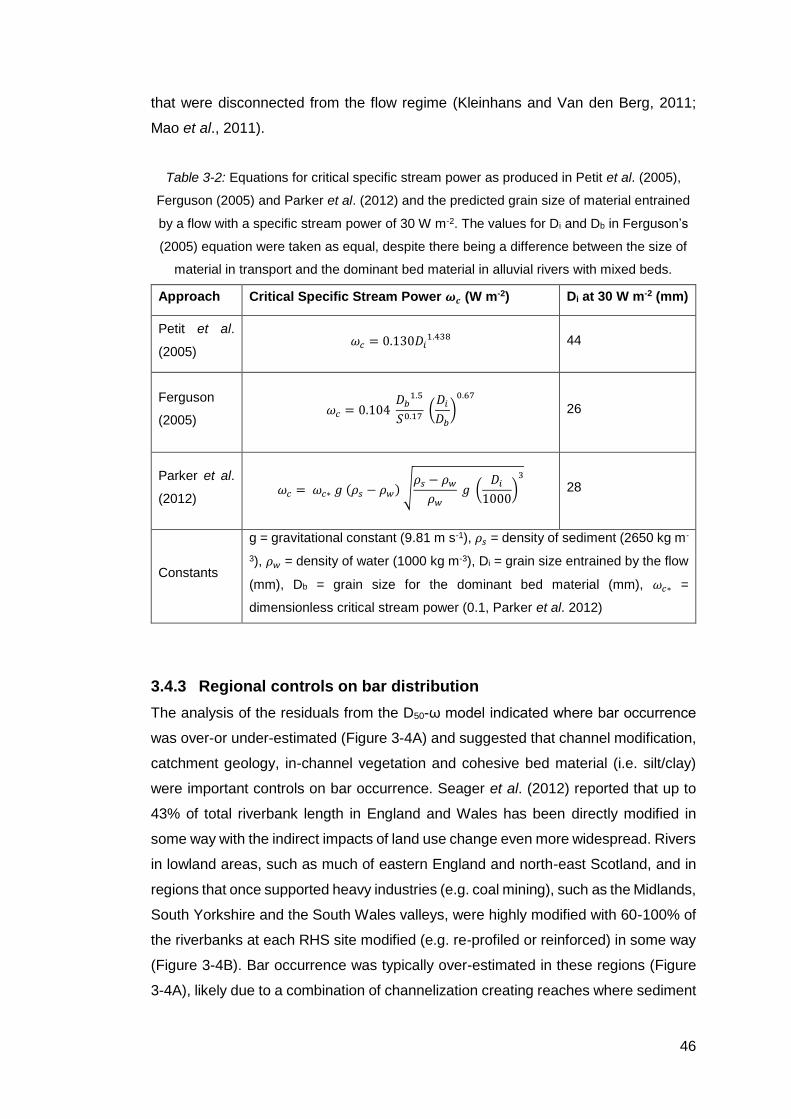
46

that were disconnected from the flow regime (Kleinhans and Van den Berg, 2011;

Mao et al., 2011).

Table 3-2: Equations for critical specific stream power as produced in Petit et al. (2005),

Ferguson (2005) and Parker et al. (2012) and the predicted grain size of material entrained

by a flow with a specific stream power of 30 W m-2. The values for Di and Db in Ferguson’s

(2005) equation were taken as equal, despite there being a difference between the size of

material in transport and the dominant bed material in alluvial rivers with mixed beds.

Approach Critical Specific Stream Power 𝝎𝒄 (W m-2) Di at 30 W m-2 (mm)

Petit et al.

(2005) 𝜔𝑐 = 0.130𝐷𝑖

1.438 44

Ferguson

(2005) 𝜔𝑐 = 0.104

𝐷𝑏1.5

𝑆0.17 (

𝐷𝑖

𝐷𝑏

)0.67

26

Parker et al.

(2012) 𝜔𝑐 = 𝜔𝑐∗ 𝑔 (𝜌𝑠 − 𝜌𝑤) √

𝜌𝑠 − 𝜌𝑤

𝜌𝑤

𝑔 (𝐷𝑖

1000)

3

28

Constants

g = gravitational constant (9.81 m s-1), 𝜌𝑠 = density of sediment (2650 kg m-

3), 𝜌𝑤 = density of water (1000 kg m-3), Di = grain size entrained by the flow

(mm), Db = grain size for the dominant bed material (mm), 𝜔𝑐∗ =

dimensionless critical stream power (0.1, Parker et al. 2012)

3.4.3 Regional controls on bar distribution

The analysis of the residuals from the D50-ω model indicated where bar occurrence

was over-or under-estimated (Figure 3-4A) and suggested that channel modification,

catchment geology, in-channel vegetation and cohesive bed material (i.e. silt/clay)

were important controls on bar occurrence. Seager et al. (2012) reported that up to

43% of total riverbank length in England and Wales has been directly modified in

some way with the indirect impacts of land use change even more widespread. Rivers

in lowland areas, such as much of eastern England and north-east Scotland, and in

regions that once supported heavy industries (e.g. coal mining), such as the Midlands,

South Yorkshire and the South Wales valleys, were highly modified with 60-100% of

the riverbanks at each RHS site modified (e.g. re-profiled or reinforced) in some way

(Figure 3-4B). Bar occurrence was typically over-estimated in these regions (Figure

3-4A), likely due to a combination of channelization creating reaches where sediment

47

is rapidly flushed through the system (Hooke, 2003), upstream impoundments create

barriers to sediment transport (Petts, 1980) and where past dredging of the channel,

to increase channel capacity for flood control or navigation, has removed the coarse

sediment required to build bar forms (Sear et al., 1995). To assess the impact of this

extensive channel modification on bar distribution, the D50-ω models for each bar type

were re-run including a term indicating the proportion of the 500m RHS reach that

was modified and then the predictions for sites with 0% and 100% modification were

compared. The extent of modification term was significant at p <0.001 in all models.

Point bar prevalence was 20% higher (0.5 vs 0.3) in fully modified sand-bed rivers

versus unmodified counterparts (Figure S2). Point bars were also up to 15% more

common in fully modified, cobble-bed rivers with ω < 30 W m-2 (Figure 3-7). Alternate

bars were up to 10% more common in modified sand-bed rivers than at unmodified

sites, whilst mid-channel bars showed no change in occurrence between unmodified

and modified sites (Figure 3-7). Sand-bed rivers are typified by dune-ripple

sequences, although channel curvature still allows forced bar forms (e.g. point bars)

to arise (Blondeaux and Seminara, 1985); this may explain why point bars are more

common in highly modified, sand-bed rivers as overall channel curvature is less likely

to be modified by human activity than smaller bank protection or in-channel changes.

Future advancements of this study should seek to test the model against an

independent data set or a subset of the RHS baseline data used to increase the

robustness of the results.

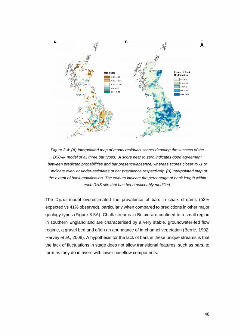
48

Figure 3-4: (A) Interpolated map of model residuals scores denoting the success of the

D50- model of all three bar types. A score near to zero indicates good agreement

between predicted probabilities and bar presence/absence, whereas scores closer to -1 or

1 indicate over- or under-estimates of bar prevalence respectively. (B) Interpolated map of

the extent of bank modification. The colours indicate the percentage of bank length within

each RHS site that has been noticeably modified.

The D50-ω model overestimated the prevalence of bars in chalk streams (52%

expected vs 41% observed), particularly when compared to predictions in other major

geology types (Figure 3-5A). Chalk streams in Britain are confined to a small region

in southern England and are characterised by a very stable, groundwater-fed flow

regime, a gravel bed and often an abundance of in-channel vegetation (Berrie, 1992;

Harvey et al., 2008). A hypothesis for the lack of bars in these unique streams is that

the lack of fluctuations in stage does not allow transitional features, such as bars, to

form as they do in rivers with lower baseflow components.

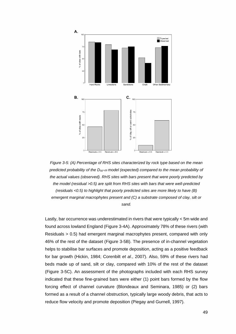
49

Figure 3-5: (A) Percentage of RHS sites characterized by rock type based on the mean

predicted probability of the D50- model (expected) compared to the mean probability of

the actual values (observed). RHS sites with bars present that were poorly predicted by

the model (residual >0.5) are split from RHS sites with bars that were well-predicted

(residuals <0.5) to highlight that poorly predicted sites are more likely to have (B)

emergent marginal macrophytes present and (C) a substrate composed of clay, silt or

sand.

Lastly, bar occurrence was underestimated in rivers that were typically < 5m wide and

found across lowland England (Figure 3-4A). Approximately 78% of these rivers (with

Residuals > 0.5) had emergent marginal macrophytes present, compared with only

46% of the rest of the dataset (Figure 3-5B). The presence of in-channel vegetation

helps to stabilise bar surfaces and promote deposition, acting as a positive feedback

for bar growth (Hickin, 1984; Corenbilt et al., 2007). Also, 59% of these rivers had

beds made up of sand, silt or clay, compared with 10% of the rest of the dataset

(Figure 3-5C). An assessment of the photographs included with each RHS survey

indicated that these fine-grained bars were either (1) point bars formed by the flow

forcing effect of channel curvature (Blondeaux and Seminara, 1985) or (2) bars

formed as a result of a channel obstruction, typically large woody debris, that acts to

reduce flow velocity and promote deposition (Piegay and Gurnell, 1997).

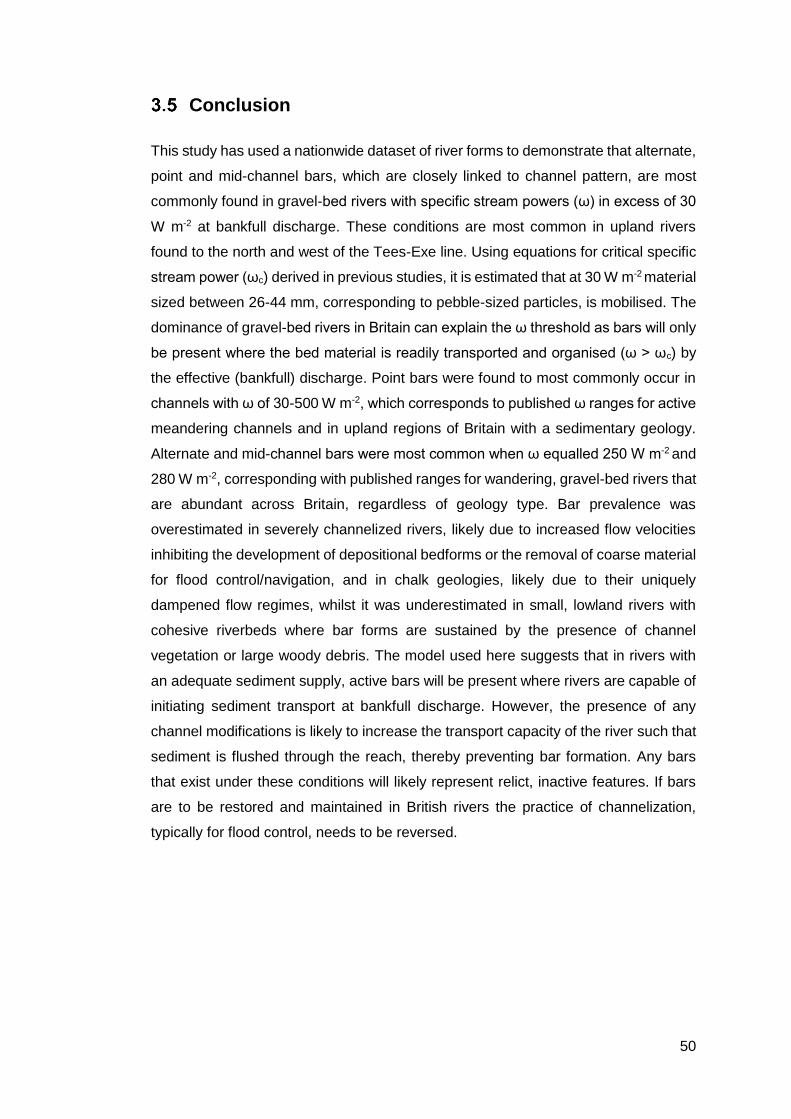
50

Conclusion

This study has used a nationwide dataset of river forms to demonstrate that alternate,

point and mid-channel bars, which are closely linked to channel pattern, are most

commonly found in gravel-bed rivers with specific stream powers (ω) in excess of 30

W m-2 at bankfull discharge. These conditions are most common in upland rivers

found to the north and west of the Tees-Exe line. Using equations for critical specific

stream power (ωc) derived in previous studies, it is estimated that at 30 W m-2 material

sized between 26-44 mm, corresponding to pebble-sized particles, is mobilised. The

dominance of gravel-bed rivers in Britain can explain the ω threshold as bars will only

be present where the bed material is readily transported and organised (ω > ωc) by

the effective (bankfull) discharge. Point bars were found to most commonly occur in

channels with ω of 30-500 W m-2, which corresponds to published ω ranges for active

meandering channels and in upland regions of Britain with a sedimentary geology.

Alternate and mid-channel bars were most common when ω equalled 250 W m-2 and

280 W m-2, corresponding with published ranges for wandering, gravel-bed rivers that

are abundant across Britain, regardless of geology type. Bar prevalence was

overestimated in severely channelized rivers, likely due to increased flow velocities

inhibiting the development of depositional bedforms or the removal of coarse material

for flood control/navigation, and in chalk geologies, likely due to their uniquely

dampened flow regimes, whilst it was underestimated in small, lowland rivers with

cohesive riverbeds where bar forms are sustained by the presence of channel

vegetation or large woody debris. The model used here suggests that in rivers with

an adequate sediment supply, active bars will be present where rivers are capable of

initiating sediment transport at bankfull discharge. However, the presence of any

channel modifications is likely to increase the transport capacity of the river such that

sediment is flushed through the reach, thereby preventing bar formation. Any bars

that exist under these conditions will likely represent relict, inactive features. If bars

are to be restored and maintained in British rivers the practice of channelization,

typically for flood control, needs to be reversed.

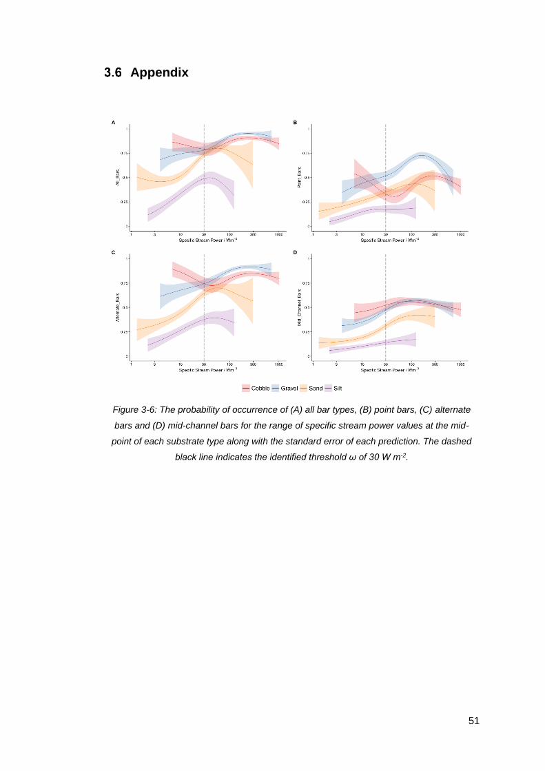
51

Appendix

Figure 3-6: The probability of occurrence of (A) all bar types, (B) point bars, (C) alternate

bars and (D) mid-channel bars for the range of specific stream power values at the mid-

point of each substrate type along with the standard error of each prediction. The dashed

black line indicates the identified threshold ω of 30 W m-2.

52

Figure 3-7: The predicted probability of occurrence of (A & B) point bars, (C & D) alternate

bars and (E & F) mid-channel bars at minimum (A, C, E) and maximum (B, D, F) channel

modification.

53

4 Effects of bed composition and stability on river

invertebrates

Abstract

Despite conceptual or descriptive studies for over a century, the interaction between

river ecology and geomorphology is still poorly understood. The role of sediment

transport in renewing habitat and acting as a disturbance to ecological communities

could be particularly important, but has never been adequately quantified. Here, I

used a unique dataset describing invertebrate communities, water quality and

hydraulic character from 714 sites across Britain to examine how physical habitat

distribution and disturbance controls invertebrate community composition.

Specifically, the Shields Regime Diagram, a simple, mechanistic model of particle

entrainment, was used to examine variations in invertebrate community composition,

function, and trait character in relation to changing estimates of substrate and

sediment transport. Invertebrate community response to disturbance varied between

rivers with gravel/cobble and silt/sand substrates. An increase in the propensity for

disturbance was found to reduce invertebrate community richness, abundance and

functional diversity in gravel/cobble substrates, with traits indicative of greater

resistance or resilience, such as short lifespans, aerial dispersal and smaller aquatic

stages also becoming more prevalent. In silt/sand substrates, patterns were more

complex as communities with highly-abundant taxa became dominant with increasing

transport ability, perhaps indicating that there are fundamental differences in what

constitutes disturbance (cf. gravel/cobble). These results are consistent with other

studies of disturbance, within rivers and in wider ecosystems, and provide further

evidence of a common response to habitat variability across ecosystems.

54

Introduction

Rivers are among the most complex and diverse environments, and as a

consequence support some of the most diverse ecological communities on Earth

(Strayer and Dudgeon, 2010). Understanding the interaction between these

communities and their habitat is a major goal in river ecology, as part of wider efforts

to reveal the drivers of biodiversity patterns in a range of ecosystems (Sala et al.,

2000). This has assumed greater importance as rivers face intensifying pressures

such as urbanisation, deforestation, hydropower development and climate change

(Dudgeon et al., 2006; Johnson et al., 2009; Vorosmarty et al., 2010; Markovic et al.,

2014; Henriuqes et al., 2015). An improved understanding of the interface between

fluvial geomorphology and river ecology will be key if freshwater communities are to

be managed for resilience in the face of these multiple pressures, yet most studies

are restricted to one of the separate disciplines (Newson and Newson, 2000;

Vaughan et al., 2009, Vaughan and Ormerod, 2010; Rice et al., 2010). Here, I use a

novel multidisciplinary approach, combining nationwide ecological sampling and a

basic model of geomorphic processes, to examine the role of the disturbance of bed

sediments on the structure and function of benthic invertebrate communities.

Interactions between geomorphology and ecology in fluvial environments are

arguably more dynamic and tightly coupled than in terrestrial environments (Fisher et

al., 2007; Corenbilt et al., 2011). This is particularly true in alluvial rivers, which are

much more common than their non-alluvial (bedrock) counterparts, with

unconsolidated sediments forming benthic habitats that are frequently redistributed

by river flow. Sediment is sorted and stacked by flow to create repeatable features in

the river channel, such as riffles, pools and bars, which support different communities

of organisms or their different life stages (Vannote et al., 1980; Poff, 1997; Benda et

al., 2004). Riffles and pools are typically found in sequence, with pools forming

narrower, deeper sections of river channel that are maintained by scouring at high

flows, and riffles forming wider, shallower sections where the largest sediment

transported by the river accumulates. Bars are the principal form of in-channel

sediment storage and themselves have a diverse range of forms, being found in

meandering and braided rivers (Chapter 3). They are responsible for much of the

habitat heterogeneity found in these systems and can support both freshwater and

terrestrial organisms (Eyre et al., 2001; Madsen et al., 2001). Together, these and

other morphological features form a dynamic ‘template’ upon which riverine

55

organisms have evolved (Townsend and Hildrew, 1994), being continually reshaped

and renewed by sediment transport initiated during high flow events.

There is a long history of descriptive studies linking river organisms to their preferred

habitats (Riley, 1921; Percival and Whitehead, 1929), yet research quantifying these

relationships is typically confined to the microhabitat scale (Jowett et al., 1991;

Statzner et al., 2000) or to single rivers (Rempel et al., 2001; Jowett, 2003). Studies

looking at larger spatial scales, producing generic theories about the geomorphology

– ecology interface, such as Vannote et al.’s (1980) River Continuum Concept or

Frissell et al.’s (1986) hierarchical view of river systems, remain conceptual and

largely qualitative. More importantly, the descriptive nature of most studies –

correlating the observed community to a static view of habitat features – provides

limited insight into the underlying mechanisms, and are likely to generalise poorly in

a changing environment: rectifying this limitation is a research priority in many

environments (Urban et al., 2016). From the geomorphic perspective, models linking

to the ecology would benefit from capturing the key controls on sediment transport in

alluvial rivers. These are primarily the flow conditions of the river and the nature (i.e.

size and shape) of the river sediment itself, which together control the morphology of

physical habitat and drive the rate at which physical habitat forms are created and

renewed in both space and time (Shields, 1936; Andrews, 1983; Parker, 1990). This

relationship between flow and sediment will determine how often the riverbed is

mobilised and transported, which directly impacts on channel form, in-channel and

riparian vegetation and presumably also on river organisms that may be inhabiting

the riverbed, through the extent of different habitats and the disturbance regime.

Concomitantly, from the biological perspective, the ability to include fundamental

processes that shape communities, such as evolution, dispersal and inter-specific

interactions, should lead to a deeper understanding and greater predictive ability

(Urban et al., 2016).

Efforts to provide a more mechanistic link between biology and the physical

environment using first principles were initiated by Southwood (1977; 1988) who

proposed that our understanding of organism-habitat relationships should focus on

the strategies employed by organisms to persist and thrive in their environments. He

argued that these strategies had a spatial and temporal component, principally related

to resource availability and stability. In river systems, Townsend and Hildrew (1994)

developed this idea into the Habitat Template Theory, which described habitats on

two conceptual axes, with a spatial axis represented by environmental heterogeneity

56

and the refugia from disturbance that such heterogeneity creates, and a temporal axis

represented by the regularity of disturbance events. These axes then provide the

template into which organisms have evolved, developing ecological traits adapted to

those conditions (Townsend and Hildrew, 1994). Poff (1997) added an explicit scale

component to the idea of a habitat template, drawing on the hierarchical view of rivers

proposed by Frissell et al. (1986), describing it as a series of filters running from basin

to microhabitat scales that organisms with specific traits have to pass through in order

to persist in an environment. In essence, many of these conceptual models recognise

the importance of riverbed sediment mobility in controlling species distributions and

community structure, yet the links are often qualitative and implicit within a larger

disturbance and heterogeneity framework.

Several previous studies have tried to directly link measures of river hydraulics or bed

mobility to the zonation of river organisms, in particular for freshwater invertebrates.

Statzner and Higler (1986) were the first to assess benthic invertebrate zonation in

relation to measures of stream hydraulics and found that in fourteen streams across

the world, changes in species assemblages were linked to changes in the hydraulics.

Death and Winterbourn (1995) and Death (1995) found, using a dataset of 11

freshwater habitats in New Zealand, that river reaches with more mobile beds were

colonised by communities with lower diversity, consisting of taxa with ecological traits

that confer resistance to, and facilitate re-colonisation after, flood events. Selecting a

measure of riverbed stability that is analogous to a disturbance episode for freshwater

invertebrates has proved tricky, with a number of different approaches proposed

including an all-encompassing sediment stability index (Schwendel et al., 2012), the

Pfankuch Index (Schwendel et al., 2010a), a measure based on the direct

measurement of tracer stone movement, and the physically based measure of shear

stress (Schwendel et al., 2010b). Many of these methods also involve labour-

intensive fieldwork, limiting the geographical scope of studies and therefore their

generality. An additional complication of linking riverbed movement and invertebrate

community composition lies in defining whether riverbed movements act directly to

remove invertebrates themselves, or indirectly, by removing their food sources such

as biofilms (Bond and Downes, 2000; Death, 2002). In part due to these challenges,

general, process-based models linking river bed dynamics and ecological community

structure are lacking, despite the empirical and conceptual developments of recent

years.

57

In ecology, the use of ecological traits (cf. taxonomy), promoted by the habitat

template theory, has driven a fruitful field of research into community structure (Poff,

1997; McGill et al., 2006; Verberk et al., 2013) that can provide greater insight into

the links between organisms and the physical environment. This trait-based approach

has the advantages of not only linking to the habitat template, but also providing a

notion of community function (e.g. by looking at feeding guilds; Poff, 1997; Lamouroux

et al., 2004) and being able to distinguish between patterns of community structure

driven by niche, as opposed to neutral mechanisms (Mouillot et al., 2013). Several

studies have looked at how traits are linked to bed composition (i.e. habitat) and

transport. For example, Demars et al. (2012) showed that river biotopes (distinct

areas of riverbed between 1-100 m2) were better predictors of macroinvertebrate trait

profiles (variance explained = 40%) than genus-level composition (variance explained

= 26%). Where riverbeds are more frequently mobilised, communities have been

found to possess traits indicative of disturbance, such as high mobility, a streamlined

body form and aerial dispersal (Townsend et al., 1997; Lobera et al., 2017). Moving

beyond the prevalence of individual traits, multivariate trait assessments have

provided new insights into communities and the assembly rules that shape them by

considering community-level functional diversity (Mouillot et al. 2013). This includes

properties such as functional richness – the full set of functional roles performed by a

community – and functional dispersion – how functionally distinct individual taxa in a

community are and to what extent they overlap with potential competitors (Mouchet

et al., 2010). Importantly, these new techniques make it possible to look at the relative

contributions of habitat filtering and inter-specific competition to community structure

(Mason et al., 2005) and lead to testable predictions. For example, highly disturbed

environments should restrict functional diversity, favouring a subset of traits that

engender resilience, whereas in more benign environments, the inter-specific

competition and limiting similarity principle may produce more functionally dispersed

communities (Mouchet et al., 2010; Mouillot et al., 2013). This approach provides new

scope for a community-level assessment of how the habitat template shapes riverine

communities.

This chapter aims to link the processes shaping organisms and communities (e.g.

evolution) with the physical processes shaping alluvial habitats (e.g. sediment type,

transport mode and frequency), based on the conceptual understanding that the

physical processes set the template upon which evolution occurs. Building on the

habitat template approach of Townsend and Hildrew (1994), this relationship is

examined at the individual taxon level, using a trait-based approach, and at the

58

community level, using both standard taxonomic metrics (e.g. richness) and

functional diversity measures of ecological communities, with a focus on traits

expected to respond to bed mobility and disturbance. Invertebrate data were obtained

from the river invertebrate prediction and classification system (RIVPACS) reference

data set, including >700 samples from rivers from across Great Britain (Davy-Bowker

et al., 2007). The invertebrate data are linked to the two axes that form the Shields

regime diagram, a simple, static model of particle entrainment based on mechanistic

first principles, which is a well-established tool in fluvial geomorphology (Parker et al.,

2003; Parker et al., 2007; Wilkerson and Parker, 2010). The first axis is the particle

Reynolds number, which describes the size of the sediment that makes up the

riverbed. whilst the second is the is the dimensionless shear stress, which describes

the propensity for riverbed movement. Together, these axes differentiate between

different geomorphic processes occurring at each location, chiefly bed-load and

suspended-load transport, and the range of substrate sizes present in the riverbed,

which in combination have been shown to control alluvial bedforms (van Rijn, 1984;

Buffington and Montgomery, 1997). I focus on the trends within substrate types (e.g.

silt, sand, gravel, cobble) as these are expected to be most reflective of where

geomorphic processes, such as bed-load transport, become active and influence on

invertebrate community composition.

Three main hypotheses are tested, predicting that invertebrate communities which

reside in more readily-disturbed riverbeds will have:

1. Lower taxonomic richness and evenness, as expected in high-disturbance

environments (Odum, 1985);

2. Lower functional richness and dissimilarity among taxa, consistent with a

strong selection pressure for traits to resist disturbance (Mason et al., 2005);

3. A greater prevalence of resistance traits, such as short lifespans, fast

reproductive cycles and aerial dispersal (Odum, 1985; Bonada et al., 2007;

Doledec et al., 2011).

Additionally, the extent to which the Shields Diagram can explain differences in two

sets of traits not explicitly linked to disturbance (feeding guilds and locomotion) will

be examined. The predicted trends in these traits are a change from traits indicative

of soft sediments (e.g. burrowing, absorbers) to hard sediments (e.g. crawling,

scrapers) as sediment calibre increases (Quinn and Hickey, 1994; Jowett, 2003).

59

Methods

4.3.1 RIVPACS dataset

The RIVPACS data set was collected between 1978 and 2002 at 725 ‘reference’ sites

deemed as being as near-natural as is possible in Britain, and contains information

on water quality, invertebrate community composition and river form (Wright et al.,

1998; 2000; Davy-Bowker et al., 2007). The dataset is particularly valuable due to its

high taxonomic resolution, standard sampling protocol and restriction to watercourses

less likely to be impacted by poor water quality and physical or catchment modification

(Murray-Bligh et al. 1997). For this study, the seasonal invertebrate sampling data

was summed into an annual dataset. The data were used at species-level for

analyses based on taxonomic metrics (e.g. richness), whilst species were combined

into genera for trait-based analyses, as this was the finest resolution at which trait

data were available (see below). Six chemical and physical variables were retained

to provide contextual information for each sampling site (Table 4-1). Eleven sites with

missing chemical and/or physical data were removed, leaving a total of 714 sites

across England, Wales and Scotland (Figure 4-2A).

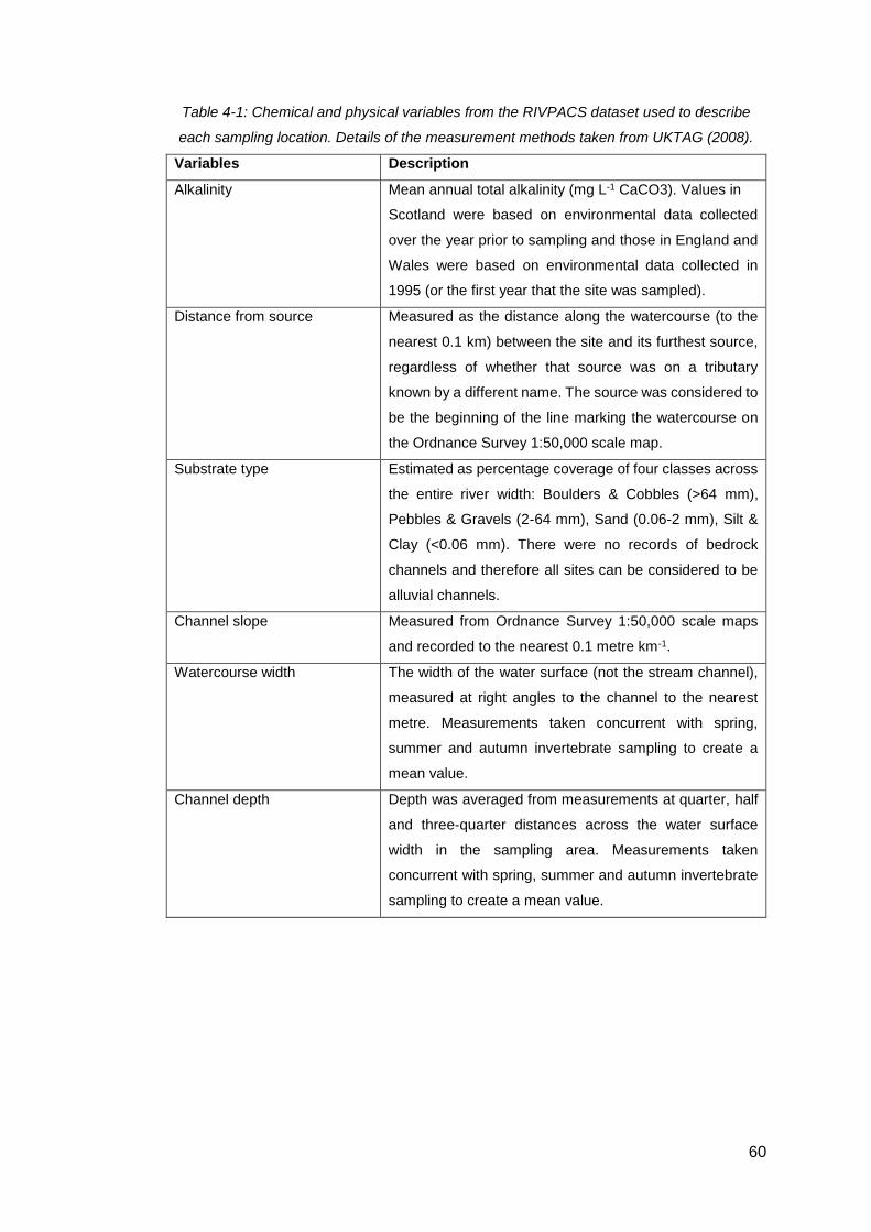
60

Table 4-1: Chemical and physical variables from the RIVPACS dataset used to describe

each sampling location. Details of the measurement methods taken from UKTAG (2008).

Variables Description

Alkalinity Mean annual total alkalinity (mg L-1 CaCO3). Values in

Scotland were based on environmental data collected

over the year prior to sampling and those in England and

Wales were based on environmental data collected in

1995 (or the first year that the site was sampled).

Distance from source Measured as the distance along the watercourse (to the

nearest 0.1 km) between the site and its furthest source,

regardless of whether that source was on a tributary

known by a different name. The source was considered to

be the beginning of the line marking the watercourse on

the Ordnance Survey 1:50,000 scale map.

Substrate type Estimated as percentage coverage of four classes across

the entire river width: Boulders & Cobbles (>64 mm),

Pebbles & Gravels (2-64 mm), Sand (0.06-2 mm), Silt &

Clay (<0.06 mm). There were no records of bedrock

channels and therefore all sites can be considered to be

alluvial channels.

Channel slope Measured from Ordnance Survey 1:50,000 scale maps

and recorded to the nearest 0.1 metre km-1.

Watercourse width The width of the water surface (not the stream channel),

measured at right angles to the channel to the nearest

metre. Measurements taken concurrent with spring,

summer and autumn invertebrate sampling to create a

mean value.

Channel depth Depth was averaged from measurements at quarter, half

and three-quarter distances across the water surface

width in the sampling area. Measurements taken

concurrent with spring, summer and autumn invertebrate

sampling to create a mean value.

61

4.3.2 Invertebrate Traits

Eight candidate ecological traits were selected from the invertebrate trait database of

Tachet et al. (2002) to describe resistance and resilience strategies (Table 4-2).

These captured traits such as lifespan, reproductive method and number of

reproductive cycles per annum, which are widely used to indicate relative resistance

and resilience (Bonada et al., 2007; Larsen and Ormerod, 2010; Doledec et al., 2011;

Gutiérrez-Cánovas et al., 2015). Although not indicative of resistance or resilience

strategies, the traits of locomotion method and feeding guild were also selected

(Table 4-2), to further assess the power of combining traits and simple geomorphic

models akin to a habitat template (Quinn and Hickey, 1994; Jowett, 2003). In the

Tachet database, each genus is assigned a fuzzy-coded score from zero to three

indicating its affinity to each individual category within each trait group (e.g. individual

scores for each reproduction method; Tachet et al., 2002). These were converted to

percentage affinity to each trait category to standardise for potential differences in the

fuzzy-coded scores (Gutierrez-Canovas et al., 2015). Individual categories for each

trait group summed to 100%.

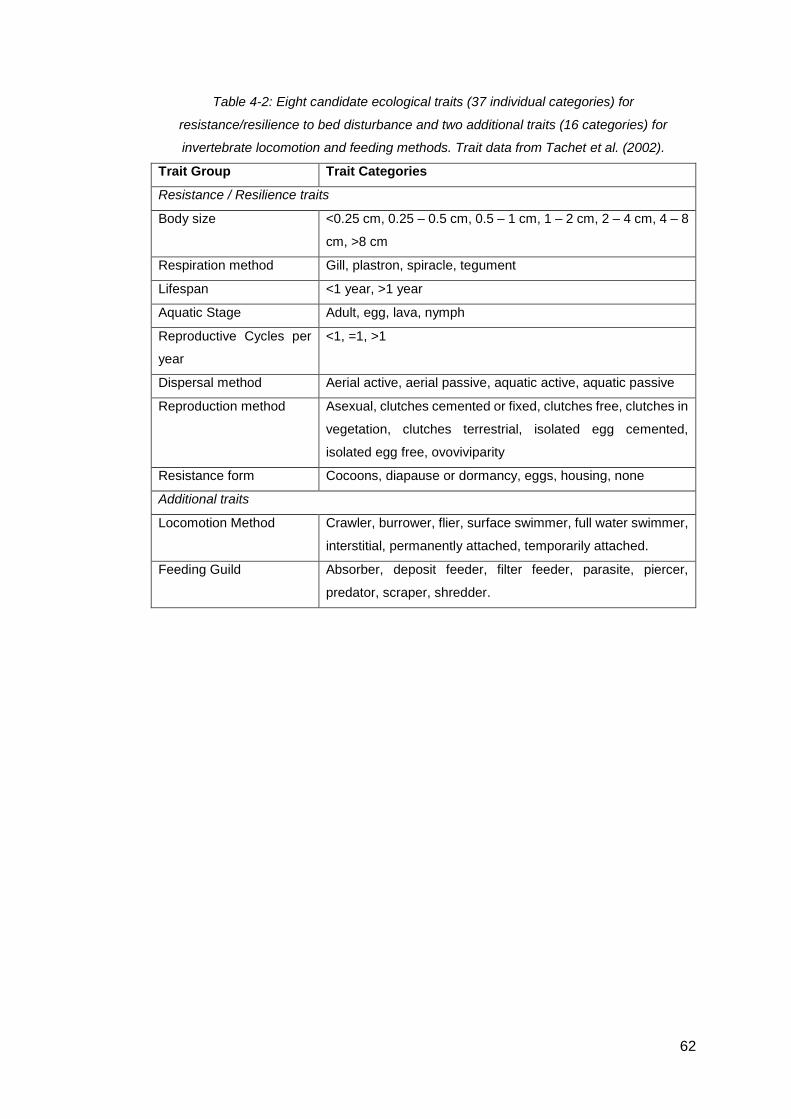
62

Table 4-2: Eight candidate ecological traits (37 individual categories) for

resistance/resilience to bed disturbance and two additional traits (16 categories) for

invertebrate locomotion and feeding methods. Trait data from Tachet et al. (2002).

Trait Group Trait Categories

Resistance / Resilience traits

Body size <0.25 cm, 0.25 – 0.5 cm, 0.5 – 1 cm, 1 – 2 cm, 2 – 4 cm, 4 – 8

cm, >8 cm

Respiration method Gill, plastron, spiracle, tegument

Lifespan <1 year, >1 year

Aquatic Stage Adult, egg, lava, nymph

Reproductive Cycles per

year

<1, =1, >1

Dispersal method Aerial active, aerial passive, aquatic active, aquatic passive

Reproduction method Asexual, clutches cemented or fixed, clutches free, clutches in

vegetation, clutches terrestrial, isolated egg cemented,

isolated egg free, ovoviviparity

Resistance form Cocoons, diapause or dormancy, eggs, housing, none

Additional traits

Locomotion Method Crawler, burrower, flier, surface swimmer, full water swimmer,

interstitial, permanently attached, temporarily attached.

Feeding Guild Absorber, deposit feeder, filter feeder, parasite, piercer,

predator, scraper, shredder.

63

4.3.3 Geomorphic Template

In alluvial rivers, riverbed sediment is transported in two main ways; as bed load,

where material rolls along the riverbed typically for relatively short distances (e.g. riffle

to riffle), or as suspended load, where material is lifted off the bed surface into the

river flow and transported over greater distances (Bagnold, 1956; Engelund and

Hansen, 1967). The dominance of each process is controlled by the depth and

velocity of flow and the calibre (principally the size) of sediment within the river

channel (Dade and Friend, 1998). For example, larger material (e.g. cobbles/pebbles)

is typically transported as bedload, whilst smaller material (e.g. sand/silt) is carried as

suspended load (Dade and Friend, 1998). As such, riverbeds composed of differing

amounts of these materials can behave very differently under flood flow conditions

(Wilcock et al., 2001; Curran and Wilcock, 2005).

To capture the two main transport mechanisms (bed load vs suspended load), along

with a measure of the propensity for riverbed movement (i.e. disturbance), the Shields

regime diagram was chosen (Shields, 1936; Figure 4-2B). In simple terms, the model

captures variation in physical habitat (through changing substrate size; x-axis of

Figure 4-2B) and disturbance regime (through changing propensity for riverbed

movement; y-axis of Figure 4-2B), whilst also providing a clear link to geomorphic

process via the laboratory defined thresholds for bed load and suspended load

transport (Andrews, 1994). Previous studies linking river hydraulics and physical

habitat have used the same or closely related measures of substrate size (e.g. D50,

Reynolds number) and flow energy (e.g. shear stress, specific stream power, Froude

number) in a similar approach (Clifford et al., 2006; Bizzi and Lerner, 2012; Vaughan

et al., 2013; Chapter 3)

4.3.3.1 Shields Regime Diagram

The Shields’ (1936) regime diagram comprises the dimensionless Shields’ number

(τ*) and the particle Reynolds number (Rep) which were defined by Parker et al.

(2003) as:

𝜏∗ =𝑑𝑆

𝑅𝐷50

𝑅𝑒𝑝 =𝐷50√𝑅𝑔𝐷50

𝜐

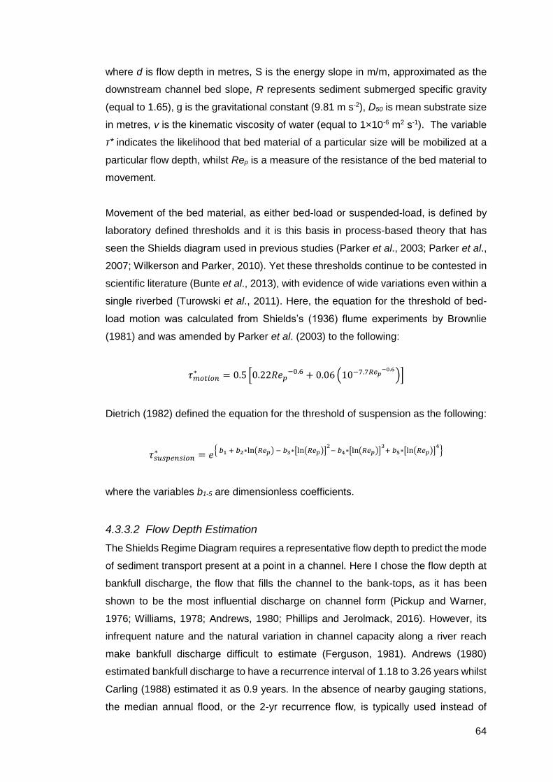
64

where d is flow depth in metres, S is the energy slope in m/m, approximated as the

downstream channel bed slope, R represents sediment submerged specific gravity

(equal to 1.65), g is the gravitational constant (9.81 m s-2), D50 is mean substrate size

in metres, ν is the kinematic viscosity of water (equal to 1×10-6 m2 s-1). The variable

τ* indicates the likelihood that bed material of a particular size will be mobilized at a

particular flow depth, whilst Rep is a measure of the resistance of the bed material to

movement.

Movement of the bed material, as either bed-load or suspended-load, is defined by

laboratory defined thresholds and it is this basis in process-based theory that has

seen the Shields diagram used in previous studies (Parker et al., 2003; Parker et al.,

2007; Wilkerson and Parker, 2010). Yet these thresholds continue to be contested in

scientific literature (Bunte et al., 2013), with evidence of wide variations even within a

single riverbed (Turowski et al., 2011). Here, the equation for the threshold of bed-

load motion was calculated from Shields’s (1936) flume experiments by Brownlie

(1981) and was amended by Parker et al. (2003) to the following:

𝜏𝑚𝑜𝑡𝑖𝑜𝑛∗ = 0.5 [0.22𝑅𝑒𝑝

−0.6 + 0.06 (10−7.7𝑅𝑒𝑝−0.6

)]

Dietrich (1982) defined the equation for the threshold of suspension as the following:

𝜏𝑠𝑢𝑠𝑝𝑒𝑛𝑠𝑖𝑜𝑛∗ = 𝑒

{ 𝑏1 + 𝑏2∗ln(𝑅𝑒𝑝) − 𝑏3∗[ln(𝑅𝑒𝑝)]2

− 𝑏4∗[ln(𝑅𝑒𝑝)]3

+ 𝑏5∗[ln(𝑅𝑒𝑝)]4

}

where the variables b1-5 are dimensionless coefficients.

4.3.3.2 Flow Depth Estimation

The Shields Regime Diagram requires a representative flow depth to predict the mode

of sediment transport present at a point in a channel. Here I chose the flow depth at

bankfull discharge, the flow that fills the channel to the bank-tops, as it has been

shown to be the most influential discharge on channel form (Pickup and Warner,

1976; Williams, 1978; Andrews, 1980; Phillips and Jerolmack, 2016). However, its

infrequent nature and the natural variation in channel capacity along a river reach

make bankfull discharge difficult to estimate (Ferguson, 1981). Andrews (1980)

estimated bankfull discharge to have a recurrence interval of 1.18 to 3.26 years whilst

Carling (1988) estimated it as 0.9 years. In the absence of nearby gauging stations,

the median annual flood, or the 2-yr recurrence flow, is typically used instead of

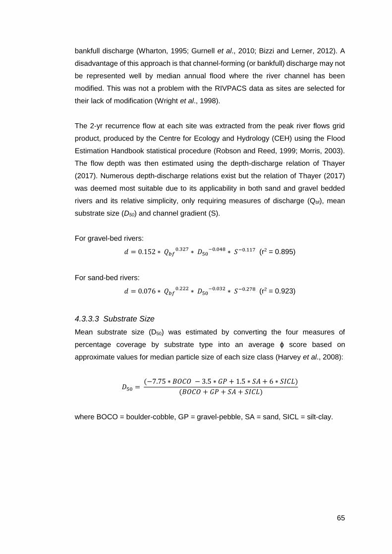
65

bankfull discharge (Wharton, 1995; Gurnell et al., 2010; Bizzi and Lerner, 2012). A

disadvantage of this approach is that channel-forming (or bankfull) discharge may not

be represented well by median annual flood where the river channel has been

modified. This was not a problem with the RIVPACS data as sites are selected for

their lack of modification (Wright et al., 1998).

The 2-yr recurrence flow at each site was extracted from the peak river flows grid

product, produced by the Centre for Ecology and Hydrology (CEH) using the Flood

Estimation Handbook statistical procedure (Robson and Reed, 1999; Morris, 2003).

The flow depth was then estimated using the depth-discharge relation of Thayer

(2017). Numerous depth-discharge relations exist but the relation of Thayer (2017)

was deemed most suitable due to its applicability in both sand and gravel bedded

rivers and its relative simplicity, only requiring measures of discharge (Qbf), mean

substrate size (D50) and channel gradient (S).

For gravel-bed rivers:

𝑑 = 0.152 ∗ 𝑄𝑏𝑓0.327 ∗ 𝐷50

−0.048 ∗ 𝑆−0.117 (r2 = 0.895)

For sand-bed rivers:

𝑑 = 0.076 ∗ 𝑄𝑏𝑓0.222 ∗ 𝐷50

−0.032 ∗ 𝑆−0.278 (r2 = 0.923)

4.3.3.3 Substrate Size

Mean substrate size (D50) was estimated by converting the four measures of

percentage coverage by substrate type into an average ɸ score based on

approximate values for median particle size of each size class (Harvey et al., 2008):

𝐷50 = (−7.75 ∗ 𝐵𝑂𝐶𝑂 − 3.5 ∗ 𝐺𝑃 + 1.5 ∗ 𝑆𝐴 + 6 ∗ 𝑆𝐼𝐶𝐿)

(𝐵𝑂𝐶𝑂 + 𝐺𝑃 + 𝑆𝐴 + 𝑆𝐼𝐶𝐿)

where BOCO = boulder-cobble, GP = gravel-pebble, SA = sand, SICL = silt-clay.

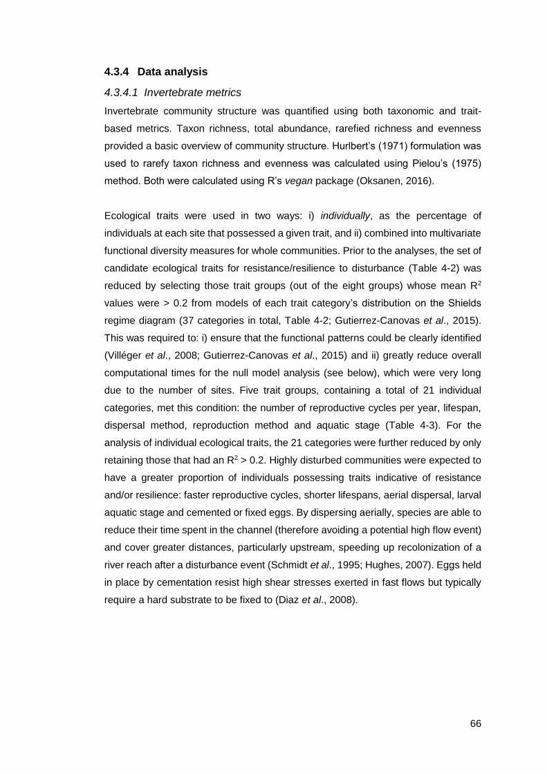
66

4.3.4 Data analysis

4.3.4.1 Invertebrate metrics

Invertebrate community structure was quantified using both taxonomic and trait-

based metrics. Taxon richness, total abundance, rarefied richness and evenness

provided a basic overview of community structure. Hurlbert’s (1971) formulation was

used to rarefy taxon richness and evenness was calculated using Pielou’s (1975)

method. Both were calculated using R’s vegan package (Oksanen, 2016).

Ecological traits were used in two ways: i) individually, as the percentage of

individuals at each site that possessed a given trait, and ii) combined into multivariate

functional diversity measures for whole communities. Prior to the analyses, the set of

candidate ecological traits for resistance/resilience to disturbance (Table 4-2) was

reduced by selecting those trait groups (out of the eight groups) whose mean R2

values were > 0.2 from models of each trait category’s distribution on the Shields

regime diagram (37 categories in total, Table 4-2; Gutierrez-Canovas et al., 2015).

This was required to: i) ensure that the functional patterns could be clearly identified

(Villéger et al., 2008; Gutierrez-Canovas et al., 2015) and ii) greatly reduce overall

computational times for the null model analysis (see below), which were very long

due to the number of sites. Five trait groups, containing a total of 21 individual

categories, met this condition: the number of reproductive cycles per year, lifespan,

dispersal method, reproduction method and aquatic stage (Table 4-3). For the

analysis of individual ecological traits, the 21 categories were further reduced by only

retaining those that had an R2 > 0.2. Highly disturbed communities were expected to

have a greater proportion of individuals possessing traits indicative of resistance

and/or resilience: faster reproductive cycles, shorter lifespans, aerial dispersal, larval

aquatic stage and cemented or fixed eggs. By dispersing aerially, species are able to

reduce their time spent in the channel (therefore avoiding a potential high flow event)

and cover greater distances, particularly upstream, speeding up recolonization of a

river reach after a disturbance event (Schmidt et al., 1995; Hughes, 2007). Eggs held

in place by cementation resist high shear stresses exerted in fast flows but typically

require a hard substrate to be fixed to (Diaz et al., 2008).

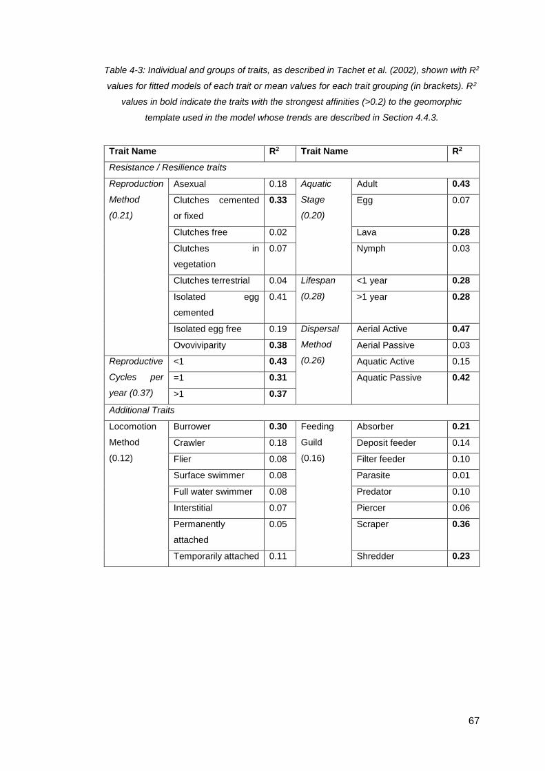
67

Table 4-3: Individual and groups of traits, as described in Tachet et al. (2002), shown with R2

values for fitted models of each trait or mean values for each trait grouping (in brackets). R2

values in bold indicate the traits with the strongest affinities (>0.2) to the geomorphic

template used in the model whose trends are described in Section 4.4.3.

Trait Name R2 Trait Name R2

Resistance / Resilience traits

Reproduction

Method

(0.21)

Asexual 0.18 Aquatic

Stage

(0.20)

Adult 0.43

Clutches cemented

or fixed

0.33 Egg 0.07

Clutches free 0.02 Lava 0.28

Clutches in

vegetation

0.07 Nymph 0.03

Clutches terrestrial 0.04 Lifespan

(0.28)

<1 year 0.28

Isolated egg

cemented

0.41 >1 year 0.28

Isolated egg free 0.19 Dispersal

Method

(0.26)

Aerial Active 0.47

Ovoviviparity 0.38 Aerial Passive 0.03

Reproductive

Cycles per

year (0.37)

<1 0.43 Aquatic Active 0.15

=1 0.31 Aquatic Passive 0.42

>1 0.37

Additional Traits

Locomotion

Method

(0.12)

Burrower 0.30 Feeding

Guild

(0.16)

Absorber 0.21

Crawler 0.18 Deposit feeder 0.14

Flier 0.08 Filter feeder 0.10

Surface swimmer 0.08 Parasite 0.01

Full water swimmer 0.08 Predator 0.10

Interstitial 0.07 Piercer 0.06

Permanently

attached

0.05 Scraper 0.36

Temporarily attached 0.11 Shredder 0.23

68

Functional diversity, the variability in a set of ecological traits at the community level,

can be summarised in a multidimensional space, known as ‘functional space’ (Villéger

et al., 2008; Mouillot et al., 2013). The functional space was created using principal

coordinates analysis (PCoA) of the ecological traits of the 242 invertebrate taxa based

on Euclidean distances (Legendre and Legendre, 1998; Villeger et al., 2008). The

number of PCoA axes retained represents the number of dimensions in which

functional space is defined (Villéger et al., 2008). A broken stick model was used to

find optimum number of PCoA axes to use to balance simplicity against the

explanatory power of the PCoA (Gutierrez-Canovas et al., 2015). Six axes, explaining

80% of the variance in the trait data, were selected for inclusion in the calculation of

functional metrics.

Three functional metrics that recognise complementary facets of functional diversity

were calculated using the FD package in R (Villéger et al., 2008; Laliberté and

Legendre 2010); (1) functional richness (FRic), a measure of the volume of functional

(trait) space occupied, (2) functional evenness (FEve), a measure of the evenness of

the distribution in macroinvertebrate abundance across the functional space and (3)

functional dispersion (FDis), the extent to which taxon abundance is spread towards

the extremes of functional space (Figure 4-1). FRic and FDis in particular are valuable

for assessing the potential assembly rules for communities (Mason et al., 2013).

Strong environmental filtering results in lower functional diversity, with reduced FRic

and lower FDis (Figure 4-1), as fitness of a taxon is maximised by being close to some

optimum (e.g. possession of a particular set of traits for withstanding bed

disturbance). With more benign conditions (e.g. less bed disturbance), fitness is

maximised by minimising potential niche overlap – hence competition – among taxa

(consistent with the limiting similarity principle; Abrams, 1983), so greater dispersion

in functional space would be expected (Mason et al., 2013; Figure 4-1).

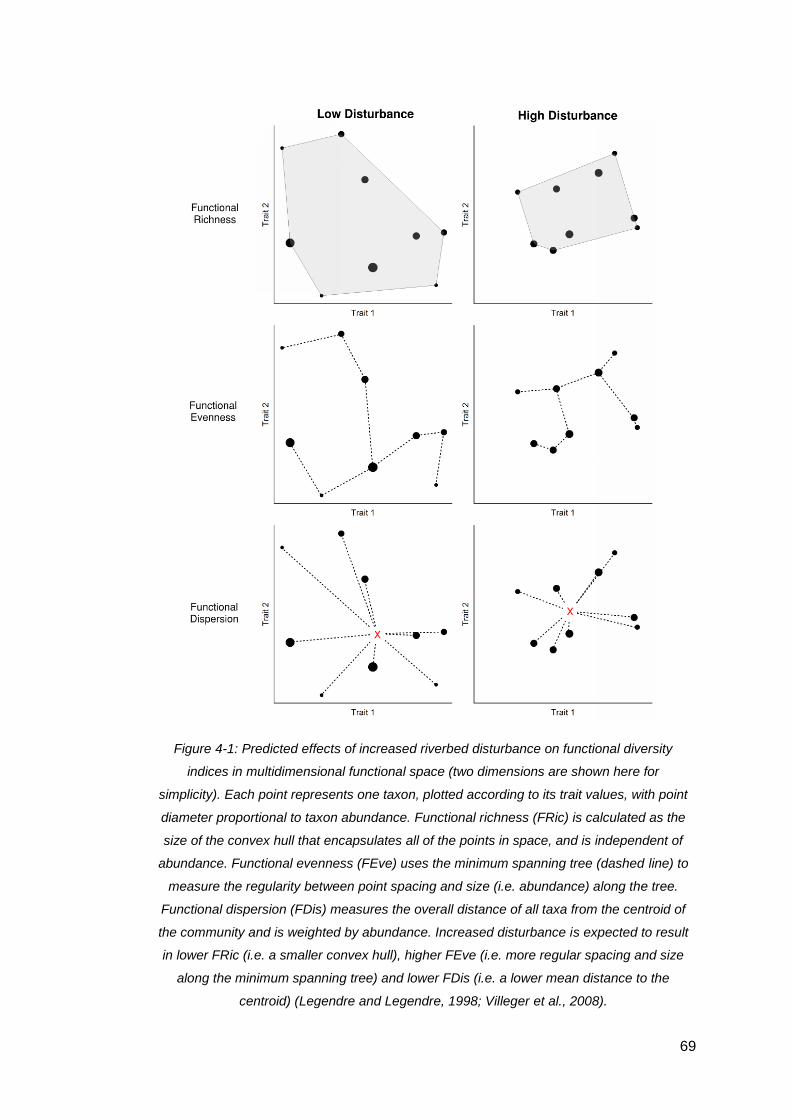
69

Figure 4-1: Predicted effects of increased riverbed disturbance on functional diversity

indices in multidimensional functional space (two dimensions are shown here for

simplicity). Each point represents one taxon, plotted according to its trait values, with point

diameter proportional to taxon abundance. Functional richness (FRic) is calculated as the

size of the convex hull that encapsulates all of the points in space, and is independent of

abundance. Functional evenness (FEve) uses the minimum spanning tree (dashed line) to

measure the regularity between point spacing and size (i.e. abundance) along the tree.

Functional dispersion (FDis) measures the overall distance of all taxa from the centroid of

the community and is weighted by abundance. Increased disturbance is expected to result

in lower FRic (i.e. a smaller convex hull), higher FEve (i.e. more regular spacing and size

along the minimum spanning tree) and lower FDis (i.e. a lower mean distance to the

centroid) (Legendre and Legendre, 1998; Villeger et al., 2008).

70

4.3.4.2 Null models

Variations in taxonomic richness, which may be sensitive to differences in abundance

among samples, can generate spurious relationships between environmental and

functional variables (Villéger et al., 2008; 2011). Null models provide a basis for

overcoming this problem, simulating the expected changes in functional diversity that

would result from varying richness, against which the observed patterns of functional

diversity can be compared. This null modelling process was used to correct FRic and

FDis for potential sampling effects: the formula for FEve makes it independent of

taxonomic richness (Villéger et al., 2008). The independent-swap method was used

to create 999 artificial site vs genera matrices from the original dataset (Gotelli, 2000;

Mason et al., 2013). Functional richness and functional dispersion were then re-

calculated for the artificial matrices at each of the 714 sites. The mean expected

values and standard deviations (from the null modelling) and the observed trends

were then used to calculate the standard effect size for the two functional metrics:

sim

simobs IISES

)(

where Iobs = observed value of the index (FRic or FDis), Isim = the mean value of the

index from the iterations of the null model and σsim = the standard deviation of the

index from the model iterations (Gotelli and McCabe, 2002). The trend in standardised

effect size can be interpreted in the same way as measures such as species richness,

whilst standard effect sizes greater than +/- 2 are deemed to exceed the approximate

95% significance level, indicating that the observed values are significantly different

to a random expectation (Mason et al., 2013). The null model adjusted values of FRic

and FDis are denoted ses.FRic and ses.FDis respectively.

4.3.4.3 Regression modelling

Community metrics, functional metrics and individual traits were modelled as a

function of τ* and Rep, the two axes of the Shield’s diagram, using generalised

additive models (GAMs) with identity links and Gaussian errors. Alkalinity, to control

for variation in water chemistry, and distance from source, to control for river size,

were also included as covariates, as these can have large effects upon the

invertebrate community (Wright et al., 1998). τ* and Rep were modelled using a tensor

product of thin-plate regression splines, whilst the other variables were modelled

using standard regression splines, with the degree of smoothing determined by

71

generalized cross validation (Wood, 2006). This approach accommodated

interactions between τ* and Rep, whilst minimizing the risks of overfitting the data by

fitting too complex a relationship (Wood, 2006; Vaughan et al., 2013). As a non-linear

method, GAM is able to detect sudden changes, such as those expected to occur at

the thresholds of bed load and suspended load transport, or a unimodal response

consistent with the intermediate disturbance hypothesis (Connell, 1978). The fit of

each model was checked by examining plots of the residuals.

To assist with interpretation of the models, predictions were generated along four

slices through the Shield’s diagram. Fixed values of Rep were used, corresponding to

rivers with substrates of cobble, gravel, sand and silt. This method allowed for

comparison between riverbeds composed of different sediment calibres, particularly

fine and coarse substrates, which are known to function in distinct ways. Riverbeds

composed of sand derive their stability principally through bedform resistance (Smith,

1970), whilst coarse riverbeds (i.e. gravel and cobble) are more reliant upon the

resistance of individual particles (Andrews, 1983). The wider gradient from coarse to

fine riverbeds is most representative of catchment position and was deemed to be

less useful for the study of the hypotheses considered here. This process which drives

this gradient is termed downstream fining, whereby particle size decreases with

distance downstream, largely due to particle abrasion and selective transport (Hoey

and Ferguson, 1994).

These slices were then plotted alongside one another to show the variation in

predicted values of the biological metrics for the different substrate types as the

propensity for disturbance increased and the transport process changed from no bed

movement towards bed load dominant to suspended load dominant. This method

simplified identification of potential nonlinear changes in community composition at

the predicted threshold values for bed and suspended load transport.

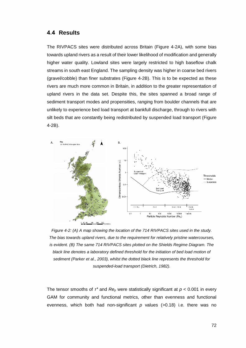
72

Results

The RIVPACS sites were distributed across Britain (Figure 4-2A), with some bias

towards upland rivers as a result of their lower likelihood of modification and generally

higher water quality. Lowland sites were largely restricted to high baseflow chalk

streams in south east England. The sampling density was higher in coarse bed rivers

(gravel/cobble) than finer substrates (Figure 4-2B). This is to be expected as these

rivers are much more common in Britain, in addition to the greater representation of

upland rivers in the data set. Despite this, the sites spanned a broad range of

sediment transport modes and propensities, ranging from boulder channels that are

unlikely to experience bed load transport at bankfull discharge, through to rivers with

silt beds that are constantly being redistributed by suspended load transport (Figure

4-2B).

Figure 4-2: (A) A map showing the location of the 714 RIVPACS sites used in the study.

The bias towards upland rivers, due to the requirement for relatively pristine watercourses,

is evident. (B) The same 714 RIVPACS sites plotted on the Shields Regime Diagram. The

black line denotes a laboratory defined threshold for the initiation of bed load motion of

sediment (Parker et al., 2003), whilst the dotted black line represents the threshold for

suspended-load transport (Dietrich, 1982).

The tensor smooths of τ* and Rep were statistically significant at p < 0.001 in every

GAM for community and functional metrics, other than evenness and functional

evenness, which both had non-significant p values (>0.18) i.e. there was no

73

systematic variation in taxonomic or functional evenness across the Shields’ diagram

(

Table 4-4). The additional predictors of alkalinity and distance from source were

significant at p < 0.01 in all models except for FDis (alkalinity p = 0.83, distance from

source p = 0.028), ses.FRic (distance from source p = 0.40) and ses.FDis (both

variables p > 0.10;

Table 4-4) but were retained in the models to simplify the interpretation of results.

4.4.1 Community metrics

The GAMs for the community metrics varied widely in their explanatory ability, from

rarefied richness (R2 = 0.10), through richness (0.35), to abundance (0.46). Overall,

increasing disturbance propensity (τ*) resulted in decreased species richness across

all substrate types, and a decrease in abundance in cobble, gravel and sand

substrates (Figure 4-3B & 4-3D). Rarefied richness showed a contrasting response

to disturbance propensity between coarse (gravel and cobble) and fine (sand and silt)

substrates, with a steep decrease with disturbance in sand and silt substrates, and

little to no change with disturbance in gravel and cobble substrates (Figure 4-3F).

In gravel to boulder substrates, species richness ranged from 66-88 yet in finer

substrates (clay to sand) a higher range of 81-96 was observed, with no evidence for

nonlinearity over the motion/suspension thresholds (Figure 4-3B). Abundance

declined with increasing disturbance propensity from 6500 to 2250 individuals per

sample in cobble substrates, with the steepest decline around the threshold of bed

load motion, and it also declined from 6600 to 4000 in gravel substrates, mirroring the

trends in species richness (Figure 4-3D). In sand substrates, no significant change

with increasing propensity for disturbance was observed and in silt substrates

abundance increased from 4800 to 7600 (Figure 4-3D). This increase in abundance

in silt-clay substrates was driven by a small number of taxa, including Potamopyrgus,

Gammarus, dipterans and oligochaetes. Species richness and abundance both

showed distinct overall minima in cobble-boulder substrates with the highest

propensity for disturbance (Figure 4-3A & 4-3C).

Rarefied richness showed little or no change with disturbance propensity in cobble or

gravel substrates (Figure 4-3F). This indicates that the observed decline in species

richness in gravel and cobble substrates was driven by a reduction in the overall

abundance of individuals i.e. a sampling effect (Magurran, 2004). Rarefied richness

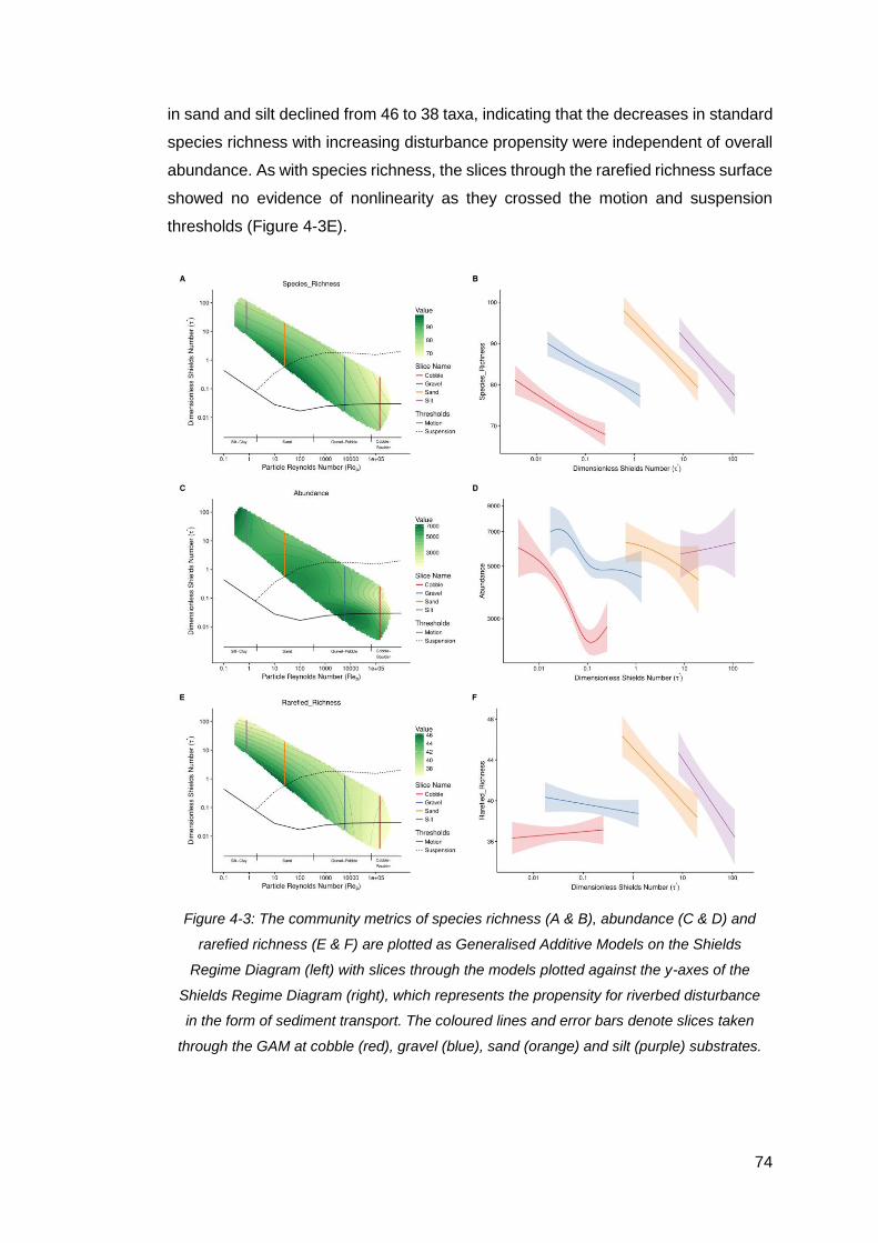
74

in sand and silt declined from 46 to 38 taxa, indicating that the decreases in standard

species richness with increasing disturbance propensity were independent of overall

abundance. As with species richness, the slices through the rarefied richness surface

showed no evidence of nonlinearity as they crossed the motion and suspension

thresholds (Figure 4-3E).

Figure 4-3: The community metrics of species richness (A & B), abundance (C & D) and

rarefied richness (E & F) are plotted as Generalised Additive Models on the Shields

Regime Diagram (left) with slices through the models plotted against the y-axes of the

Shields Regime Diagram (right), which represents the propensity for riverbed disturbance

in the form of sediment transport. The coloured lines and error bars denote slices taken

through the GAM at cobble (red), gravel (blue), sand (orange) and silt (purple) substrates.

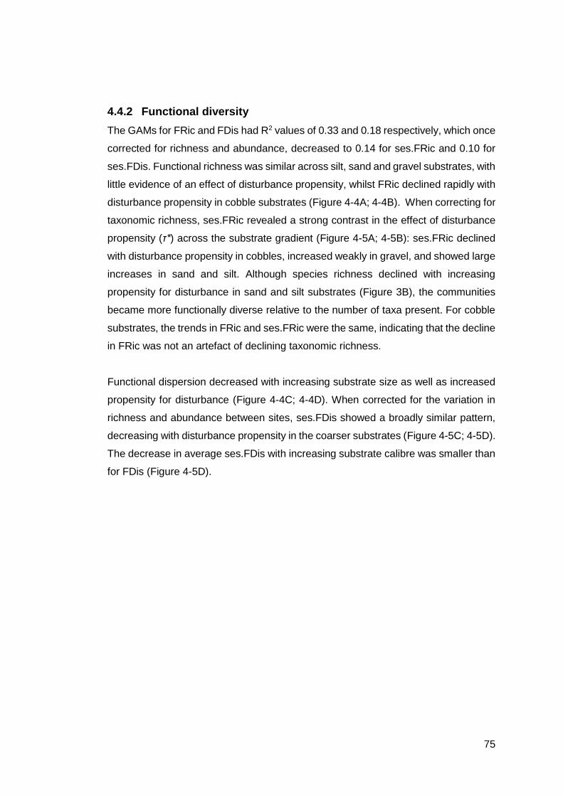
75

4.4.2 Functional diversity

The GAMs for FRic and FDis had R2 values of 0.33 and 0.18 respectively, which once

corrected for richness and abundance, decreased to 0.14 for ses.FRic and 0.10 for

ses.FDis. Functional richness was similar across silt, sand and gravel substrates, with

little evidence of an effect of disturbance propensity, whilst FRic declined rapidly with

disturbance propensity in cobble substrates (Figure 4-4A; 4-4B). When correcting for

taxonomic richness, ses.FRic revealed a strong contrast in the effect of disturbance

propensity (τ*) across the substrate gradient (Figure 4-5A; 4-5B): ses.FRic declined

with disturbance propensity in cobbles, increased weakly in gravel, and showed large

increases in sand and silt. Although species richness declined with increasing

propensity for disturbance in sand and silt substrates (Figure 3B), the communities

became more functionally diverse relative to the number of taxa present. For cobble

substrates, the trends in FRic and ses.FRic were the same, indicating that the decline

in FRic was not an artefact of declining taxonomic richness.

Functional dispersion decreased with increasing substrate size as well as increased

propensity for disturbance (Figure 4-4C; 4-4D). When corrected for the variation in

richness and abundance between sites, ses.FDis showed a broadly similar pattern,

decreasing with disturbance propensity in the coarser substrates (Figure 4-5C; 4-5D).

The decrease in average ses.FDis with increasing substrate calibre was smaller than

for FDis (Figure 4-5D).

76

Figure 4-4: The metrics of functional richness (FRic; A & B) and functional dispersion

(FDis; C & D) are plotted as Generalised Additive Models on the Shields Regime Diagram

(left) with slices through the models plotted against the y-axes of the Shields Regime

Diagram (right), which represents the propensity for riverbed disturbance in the form of

sediment transport. The coloured lines and error bars denote slices taken through the

GAM at cobble (red), gravel (blue), sand (orange) and silt (purple) substrates.

77

Figure 4-5: Null models of functional richness (A & B; ses.FRic) and functional dispersion

(C & D; ses.FDis) are plotted as Generalised Additive Models with a diverging colour

gradient on the Shields Regime Diagram (left). The dashed grey lines are thresholds of +/-

0.2 which indicate the approximate 5% significance level and are deemed as significantly

different to the random expectation (Mason et al., 2013). Slices through the models are

plotted against Dimensionless Shields Number (right) which represents the propensity for

riverbed disturbance in the form of sediment transport. The coloured lines and error bars

denote slices taken through the GAM at cobble (red), gravel (blue), sand (orange) and silt

(purple) substrates.

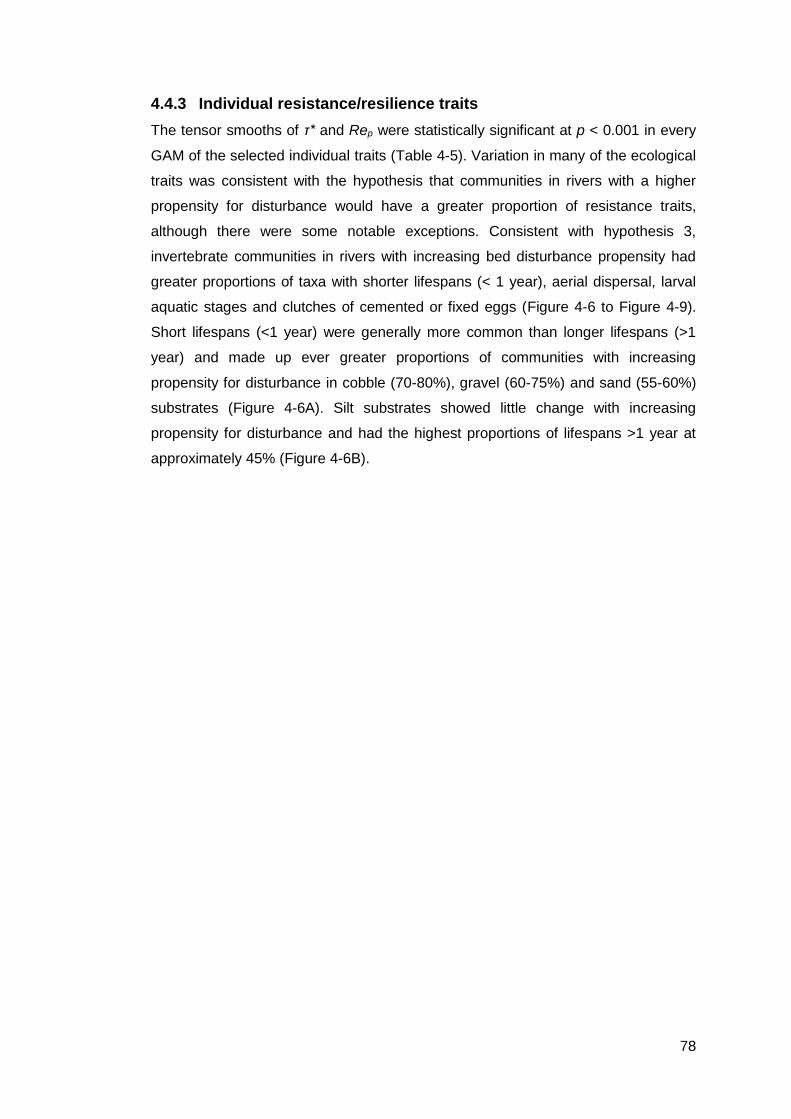
78

4.4.3 Individual resistance/resilience traits

The tensor smooths of τ* and Rep were statistically significant at p < 0.001 in every

GAM of the selected individual traits (Table 4-5). Variation in many of the ecological

traits was consistent with the hypothesis that communities in rivers with a higher

propensity for disturbance would have a greater proportion of resistance traits,

although there were some notable exceptions. Consistent with hypothesis 3,

invertebrate communities in rivers with increasing bed disturbance propensity had

greater proportions of taxa with shorter lifespans (< 1 year), aerial dispersal, larval

aquatic stages and clutches of cemented or fixed eggs (Figure 4-6 to Figure 4-9).

Short lifespans (<1 year) were generally more common than longer lifespans (>1

year) and made up ever greater proportions of communities with increasing

propensity for disturbance in cobble (70-80%), gravel (60-75%) and sand (55-60%)

substrates (Figure 4-6A). Silt substrates showed little change with increasing

propensity for disturbance and had the highest proportions of lifespans >1 year at

approximately 45% (Figure 4-6B).

79

Figure 4-6: The proportion of an invertebrate community with lifespans of (A) <1 year and

(B) >1 year, plotted against a measure of propensity for disturbance (Dimensionless

Shear Stress - τ*). The coloured lines and error bars denote slices taken through the GAM

at cobble (red), gravel (blue), sand (orange) and silt (purple) substrates.

The proportion of individuals that passively dispersed in the water column declined

with increasing disturbance propensity in all substrates and ranged from 55% of a

community in silt substrates to 35% in cobble substrates (Figure 4-7A). Conversely,

the proportion of individuals with the aerial active dispersal method increased with

increasing propensity for disturbance in all substrates and ranged from 26% of a

community in highly-disturbed cobble substrates to <15% in low disturbance silt

substrates (Figure 4-7B).

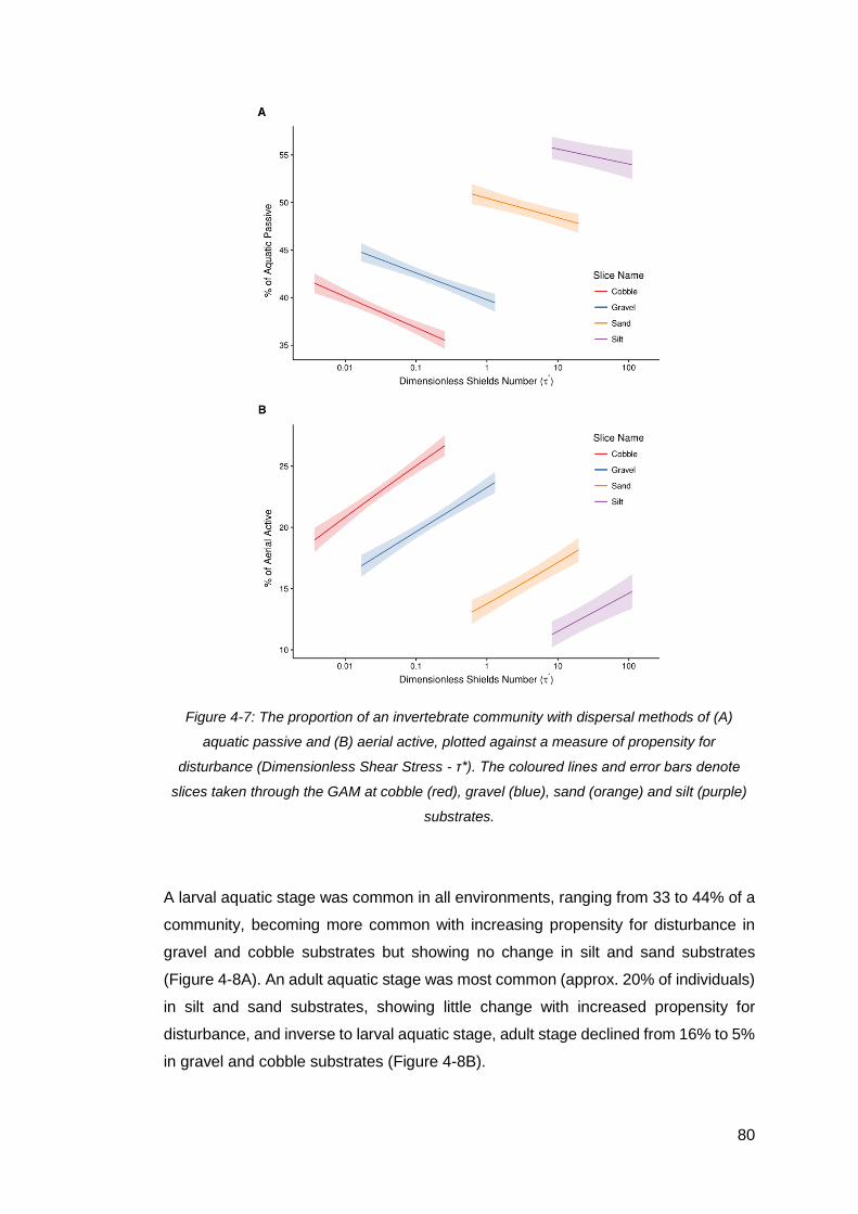
80

Figure 4-7: The proportion of an invertebrate community with dispersal methods of (A)

aquatic passive and (B) aerial active, plotted against a measure of propensity for

disturbance (Dimensionless Shear Stress - τ*). The coloured lines and error bars denote

slices taken through the GAM at cobble (red), gravel (blue), sand (orange) and silt (purple)

substrates.

A larval aquatic stage was common in all environments, ranging from 33 to 44% of a

community, becoming more common with increasing propensity for disturbance in

gravel and cobble substrates but showing no change in silt and sand substrates

(Figure 4-8A). An adult aquatic stage was most common (approx. 20% of individuals)

in silt and sand substrates, showing little change with increased propensity for

disturbance, and inverse to larval aquatic stage, adult stage declined from 16% to 5%

in gravel and cobble substrates (Figure 4-8B).

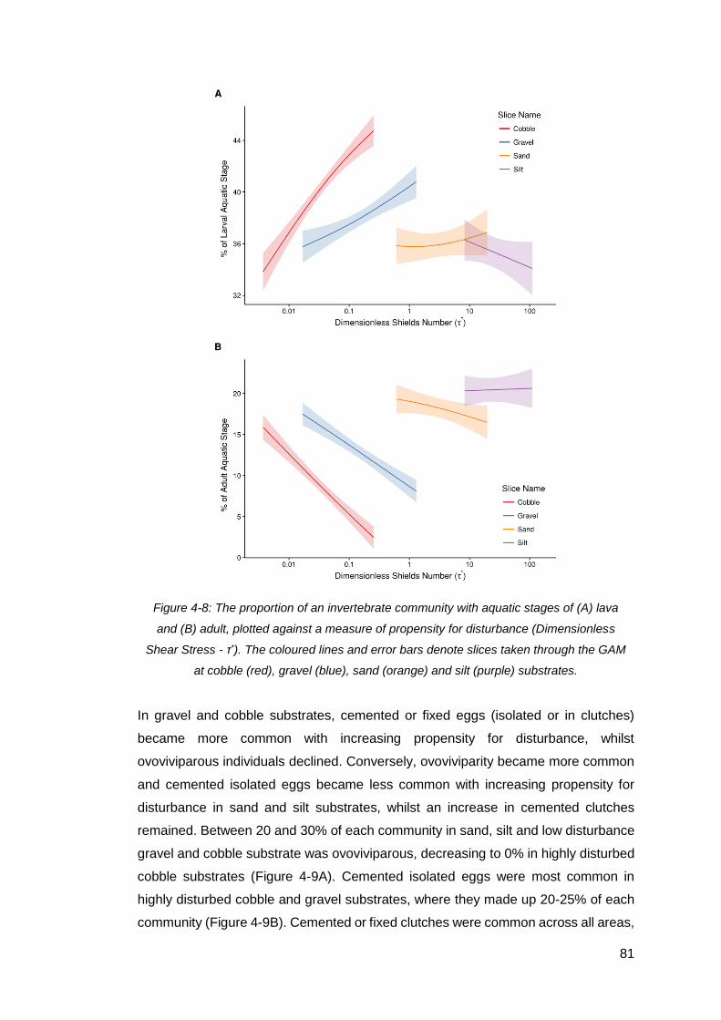
81

Figure 4-8: The proportion of an invertebrate community with aquatic stages of (A) lava

and (B) adult, plotted against a measure of propensity for disturbance (Dimensionless

Shear Stress - τ*). The coloured lines and error bars denote slices taken through the GAM

at cobble (red), gravel (blue), sand (orange) and silt (purple) substrates.

In gravel and cobble substrates, cemented or fixed eggs (isolated or in clutches)

became more common with increasing propensity for disturbance, whilst

ovoviviparous individuals declined. Conversely, ovoviviparity became more common

and cemented isolated eggs became less common with increasing propensity for

disturbance in sand and silt substrates, whilst an increase in cemented clutches

remained. Between 20 and 30% of each community in sand, silt and low disturbance

gravel and cobble substrate was ovoviviparous, decreasing to 0% in highly disturbed

cobble substrates (Figure 4-9A). Cemented isolated eggs were most common in

highly disturbed cobble and gravel substrates, where they made up 20-25% of each

community (Figure 4-9B). Cemented or fixed clutches were common across all areas,

82

making up 30% of communities in low disturbance silt substrates and up to 50% of

communities in highly disturbed cobble substrates (Figure 4-9C). Reproduction by

eggs was more common in coarse substrates, whilst ovoviviparity was more common

in fine substrates.

Figure 4-9: The proportion of an invertebrate community with reproduction method of (A)

ovoviviparity, (B) isolated cemented eggs and (C) clutches – cemented or fixed, plotted

against a measure of propensity for disturbance (Dimensionless Shear Stress - τ*). The

coloured lines and error bars denote slices taken through the GAM at cobble (red), gravel

(blue), sand (orange) and silt (purple) substrates.

83

Slow reproductive cycles (<1 per annum) were rare (always ≤8% of the community)

and had a complex relationship with increasing disturbance propensity. In cobble

substrates, the proportion increased from 2 to 8% of the community and peaked at

the threshold for bedload transport, whilst gravel substrates showed no clear trend

and sand or silt substrates showed a decreasing trend (Figure 4-10A). Thus, the

increase in slower reproductive cycles with increasing propensity for disturbance was

driven by single (=1) reproductive cycles per annum becoming more common and a

corresponding reduction in the proportion of communities with multiple cycles per

annum (Figure 4-10B; 4-10C). Despite this, multiple reproductive cycles per annum

composed >50% of every community across all substrates and disturbance

propensities, other than cobble substrates with a high propensity for disturbance,

where one cycle per annum was the most common (Figure 4-10B; 4-10C).

84

Figure 4-10: The proportion of an invertebrate community with reproductive cycles of (A)

<1 cycle p/y, (B) 1 cycle p/y and (C) >1 cycle p/y, plotted against a measure of propensity

for disturbance (Dimensionless Shear Stress - τ*). The coloured lines and error bars

denote slices taken through the GAM at cobble (red), gravel (blue), sand (orange) and silt

(purple) substrates.

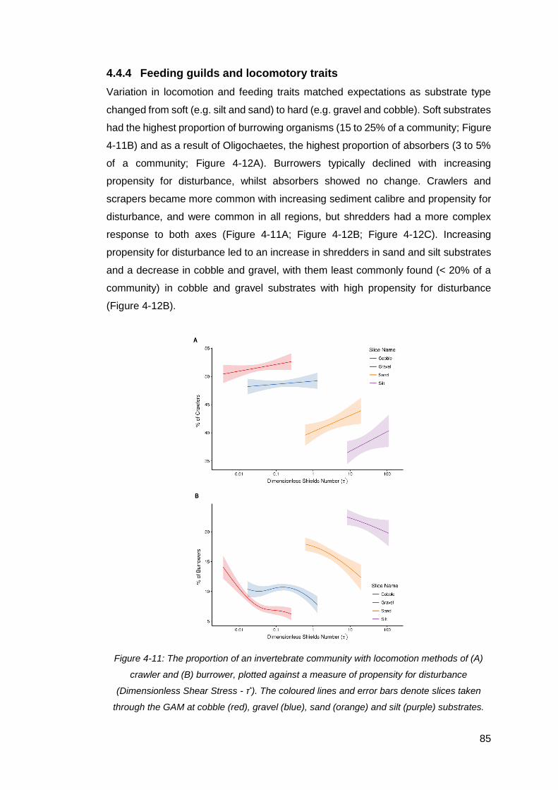
85

4.4.4 Feeding guilds and locomotory traits

Variation in locomotion and feeding traits matched expectations as substrate type

changed from soft (e.g. silt and sand) to hard (e.g. gravel and cobble). Soft substrates

had the highest proportion of burrowing organisms (15 to 25% of a community; Figure

4-11B) and as a result of Oligochaetes, the highest proportion of absorbers (3 to 5%

of a community; Figure 4-12A). Burrowers typically declined with increasing

propensity for disturbance, whilst absorbers showed no change. Crawlers and

scrapers became more common with increasing sediment calibre and propensity for

disturbance, and were common in all regions, but shredders had a more complex

response to both axes (Figure 4-11A; Figure 4-12B; Figure 4-12C). Increasing

propensity for disturbance led to an increase in shredders in sand and silt substrates

and a decrease in cobble and gravel, with them least commonly found (< 20% of a

community) in cobble and gravel substrates with high propensity for disturbance

(Figure 4-12B).

Figure 4-11: The proportion of an invertebrate community with locomotion methods of (A)

crawler and (B) burrower, plotted against a measure of propensity for disturbance

(Dimensionless Shear Stress - τ*). The coloured lines and error bars denote slices taken

through the GAM at cobble (red), gravel (blue), sand (orange) and silt (purple) substrates.

86

Figure 4-12: The proportion of an invertebrate community with feeding methods of (A)

absorber, (B) shredders and (C) scrapers, plotted against a measure of propensity for

disturbance (Dimensionless Shear Stress - τ*). The coloured lines and error bars denote

slices taken through the GAM at cobble (red), gravel (blue), sand (orange) and silt (purple)

substrates.

87

Discussion

Understanding the interactions between physical habitat and biodiversity is important

and understanding at sufficient scales to inform river management is vital if

mitigations or adaptations to future change are to be successful. At present, due to

resource and data limitations, studies have been restricted to small scales or simply

correlate observed organisms to simple measures of observed habitat e.g. current

bed material composition (e.g. Death and Winterbourn, 1995; Townsend et al., 1997).

This study has combined a large, national-scale data set with a simple, static model

of particle entrainment based on mechanistic first principles to link physical habitat

with benthic community composition in UK rivers. The model was selected due to its

low data requirements and solid grounding in past studies and theory (Parker et al.,

2003; Parker et al., 2007; Wilkerson and Parker, 2010). Whilst more mechanistic

modelling is desirable (Meyer-Peter and Muller, 1948; Wilcock and Crowe, 2003), the

requisite data are typically more difficult to obtain, particularly at the national scale

considered here. The adoption of the Shields’ diagram is a first, pragmatic step

towards more mechanistic modelling. Here I discuss key limitations of the study

before discussing the results in detail.

4.5.1 Limitations

There were four important limitations to this study, namely the reliance on secondary

data and current trait information, the inability to account for outside factors that also

control invertebrate communities (e.g. climate, resource availability, competition) and

the lack of field verification of dimensionless shear stress.

Firstly, in spite of the strengths of the RIVAPCS data set (e.g. sample size, taxonomic

resolution), the use of secondary data has a number of limitations (Vaughan and

Ormerod, 2010), which here included (1) the under-representation of lowland

watercourses as RIVPACS selects pristine sites it is inherently biased to upland areas

(Figure 4-2A), and (2) restrictions on the quality of available data for water quality and

channel morphology. The use of the Shields Regime Diagram as a representation of

the range of the channel morphologies present in the dataset introduced a reliance

on the various components used to calculate τ* and Rep, which make up the axes of

the Shields Regime diagram. The components, namely flow depth, bankfull

discharge, channel bed slope and median surface grain size, were all estimates and

potential error in each of these has scope to introduce a significant composite error.

88

The potential sources of error in the components and how these have been

considered in this study are discussed below:

1. Flow Depth: This estimation was reliant upon the relations of Thayer (2016),

which themselves were reliant upon the estimation of bankfull discharge and

slope. Thayer (2016) demonstrated that the depth relations for gravel and

sand bed rivers were more accurate than existing relations. In a test of the

relations using independent data, they found that the median value of the

depth predictions was 1.61% and 2.48% lower than the actual values for

gravel and sand bed rivers respectively (see Table 2 from Thayer, 2016).

2. Bankfull Discharge: Taken as the 2-year recurrence flow from the CEH peak

river flows grid product which itself is estimated using the Flood Estimation

Handbook (FEH) statistical procedure (Kjeldsen et al., 2008). This method

introduces two types of potential error, the accuracy of the statistical method

for deriving peak flows and the applicability of using the 2-year recurrence flow

as a proxy for bankfull discharge. The accuracy of the FEH procedure for

estimating peak flows was tested by Calver et al. (2009) who found that at 2-

year recurrence flows, estimations were within +/- 30% of gauged flows. The

applicability of using the 2-year recurrence flow is discussed in Section

4.3.3.2.

3. Channel Slope: Included in the RIVPACS dataset and calculated from the

contours on a 1:50000 map. The estimation of channel slope from digital

elevation model derived contours has been shown to be very sensitive to the

elevation data and the calculation of channel length (Jain et al., 2006; Neeson

et al., 2011). Given the relatively large scale of the mapping used to derive

channel slope, estimates are likely to be most accurate in larger rivers where

the true channel length is best represented. In smaller rivers, the channel

length is likely to be under-estimated (leading to an over-estimation of slope)

as the complexity of a small meandering channel would be under represented

by the ‘blue-line’ shown on the mapping.

4. Median Substrate Size (D50): The estimation of D50 using the four groups of

sediment type (silt, sand, gravel-pebble, cobble-boulder) would introduce

error as the potential variation in grain size is minimised using this approach.

Given that improved data is not available at this scale it is difficult to attribute

a proportion of error to the data. The estimation of riverbed substrate size

could be improved by using pebble counts or sediment sieving, which would

have provided greater accuracy.

89

Each of these estimated components was assessed visually to ensure that range of

values were sensible prior to their use.

The second limitation of the study was the trait database (Tachet et al., 2002) used

to assign traits to invertebrate taxa, which is limited by (1) the understanding of the

life-history of each taxa, as some are better studied and understood than others and

(2) where taxa have multiple abilities within a single trait category, often due to them

possessing different traits at different life stages. This lack of understanding and/or

clarity may mask some trends in the distribution of trait data.

Thirdly, a range of other factors that could influence the macroinvertebrate community

(e.g. climate) will vary simultaneously with bed material and disturbance patterns

across the country. This is consistent with the low variances explained by the models

(all < 50%), common problem with ecological models (Moller and Jennions, 2002).

The inclusion of distance from source in all of the models was intended to account for

changes in river size (i.e. available habitat) but the geographic distribution in the

dataset, ranging from upland, high-energy Scottish rivers, through to lowland, low-

energy chalk rivers in South-East England and the subsequent differences in climate

and resource availability (e.g. food, nutrients) would not have been accounted for

(Ferreira and Chauvet, 2011). Alkalinity was included in the models to broadly

account for variations in water quality but a host of other water quality variables (e.g.

temperature, phosphate, BOD, fine sediments) are known to also strongly influence

community distribution (Quinn et al, 1997; Vaughan and Ormerod, 2014). It is

therefore difficult to confidently assume that some of the trends along the disturbance

gradient are not trends in competition, resource availability, water quality or climate

impacts, which are all known to strongly influence community composition. This is

particularly true for cobble substrates as the majority of sites with a high propensity

for disturbance are high-energy, upland rivers in the most northerly areas of Britain

(i.e. Scotland), where resource availability and climatic conditions (e.g. temperature,

sunlight) would be at their lowest and harshest respectively. Despite this, functional

metrics are known to be more closely aligned to environmental conditions than

traditional community metrics and are therefore expected to offer greater insight into

ecology-geomorphology interaction (Naeem et al., 2012).

Finally, dimensionless shear stress, the measure termed as propensity for

disturbance in the model used here, has received little field validation (Whiting and

90

Dietrich, 1990) with previous studies being limited to empirical models (Parker et al.,

2003) or laboratory flumes (Petit, 1994). There is therefore some uncertainty of how

accurate the modelled thresholds are in natural riverbeds. These considerations

would, however, require extensive field testing and were beyond the scope of this

study.

4.5.2 Effects of disturbance and substrate type on invertebrate

community composition and function

The within-substrate trends shown here have provided qualified support for the

original hypotheses that invertebrate communities would respond to increasing

propensity for riverbed disturbance by becoming less diverse (taxonomically and

functionally; hypotheses one and two) and would show a general homogenisation

around traits associated with resistance and/or resilience (hypothesis three). This is

in broad agreement with other studies of freshwater invertebrate community response

to natural and anthropogenic stressors, including drought, land use, sedimentation

and salinity (Bonada et al., 2007; Larsen and Ormerod, 2010; Gutiérrez-Cánovas et

al., 2015), and to previous small-scale studies looking at river bed mobility (Death,

1995; Death and Winterbourn, 1995; Townsend et al., 1997). Yet overall trends in

species richness (Figure 4-3B) and functional dispersion (Figure 4-4D) do not support

these hypotheses, although these gradients are representative of a shift from upland

to lowland channels (coarse to fine grained sediments), rather than gradients of

varying disturbance. By combining traditional taxonomic metrics and trait-based

approaches using single-traits and functional diversity metrics, the results offer

stronger support for the role of riverbed stability in structuring invertebrate community

composition. This relationship differed by bed material type, with a marked difference

in response to increasing disturbance propensity between communities in gravel or

cobble substrates and those in sand or silt substrates. The response in gravel and

cobble substrates broadly supported all three hypotheses, whilst sand and silt

substrates often contradicted this response, with limited support for hypothesis one

(lower taxonomic richness), and little support for hypotheses two and three.

With increasing disturbance in sand and silt substrates, richness decreased whilst

overall abundance decreased in sand but increased in silt as taxa including

Potamopyrgus, Gammarus, dipterans and various oligochaetes came to dominate.

Conversely, trait composition became more diverse (increasing ses.FRic), with many

traits indicative of resistance/resilience (short lifespan, multiple reproductive cycles)

91

showing little change across the disturbance gradient, whilst others (active aerial

dispersal) increased. A potential explanation for this trend in functional richness in

sand and silt substrates is the role of inter-specific competition, as predicted by the

Habitat Template Theory (Townsend and Hildrew, 1994). If applying the theory,

communities in this habitat would place high on the temporal disturbance axis but low

on the spatial heterogeneity axis, resulting in disturbance having a greater role in

controlling community composition than resource competition between species. In

less disturbed areas, high competition for resources would limit the functional

richness of a community as species with less suitable traits would be excluded by

species with more suitable traits (Menge and Sutherland, 1987; Power et al., 1988).

Another possible explanation is the role of mass effects, where high dispersal

between local communities can alter apparent responses to local habitat (i.e.

disturbance). In this scenario, poorly-adapted species immigrate into an area from

less-disturbed habitats (e.g. channel margins, riparian zones, nearby tributaries),

which would add a small number of species at low abundance to highly disturbed

silt/sand substrates. Although only at low abundance, these additional species would

increase ses.FRic, which ignores abundance, and have little effect on ses.FDis, which

incorporates abundance. The increase in active aerial dispersal across the

disturbance gradient in silt/sand substrates offers support that mass effects are most

active in this portion of the model.

In gravel and cobble substrates rarefied richness showed no change with increasing

disturbance, highlighting that the decline in species richness was an artefact of

decreasing abundance. Trait diversity declined in cobble substrates, whilst ses.FRic

showed little change in gravel substrates, and traits such as short lifespans, larval

aquatic stage, active aerial dispersal and cemented eggs became more prevalent

with disturbance in both substrates. Ses.FDis declined with increasing disturbance in

cobble and gravel, consistent with an increasing role for environmental filtering over

interspecific competition, in support of hypothesis 2 and previous studies (Mason et

al., 2005, Mouchet et al., 2010; Mouillot et al., 2013). This was a much larger effect

than in silt or sand, where inter-specific competition appears to increase in importance

relative to environmental filtering. These trends in community and trait diversity are in

close agreement with the results of previous studies of invertebrate response to

riverbed disturbance (Reice, 1985; Death and Winterbourn, 1995; Death and

Zimmermann, 2005), which have all focussed on coarse-bedded rivers (i.e. riverbeds

made up principally of gravels and/or cobbles).

92

Disturbance is a multidimensional concept including frequency, intensity and period,

and theoretical work indicates that different combinations of disturbance frequency

and intensity can produce qualitatively different responses (Miller et al., 2010). Here,

this concept is consistent with the difference in response between communities in

sand/silt substrates and gravel/cobble substrates, which can, at least partly, be

attributed to differences in frequency and mode of sediment transport in these

systems. In rivers with silt and sand substrates, material is regularly transported in

suspension by flows at or below bankfull, whereas in coarse substrates, there is a

much greater range in transport frequency across the spectrum of sediment calibre,

with some substrates very rarely experiencing bed load transport and others

frequently being reworked by flow that approximates bankfull discharge (Turowski et

al., 2010). The regularity of bed disturbance and sediment transport in sand and silt

systems may be such that it forms the baseline condition and therefore does not act

as a disturbance to a community in the same manner as it does in rivers with gravel

or cobble substrates. In essence, the taxa adapted to this environment are capable

of thriving, particularly with a reduction in potential inter-specific competition, whereas

in high-energy gravel or cobble bed rivers communities can only persist (rather than

thrive) due to other resource constraints (Vannote et al., 1980). An example of such

taxa is Potamopyrgus antipodarum, an invasive species in the UK, which occurs in

very high densities and uses its high tolerance of siltation as a competitive advantage

(Alonso and Castro-Diez, 2008).

In most instances there was no evidence that the invertebrate community varied non-

linearly with bed disturbance, showing neither a unimodal response for richness –

consistent with the intermediate disturbance hypothesis (Connell, 1978) – nor a sharp

change in slope around the threshold between bed and suspended load: the

relationship selected by generalised cross validation when fitting the GAMs indicated

linear relationships. The latter may have been confounded by the estimated locations

of the transport threshold. Only the slices taken through cobble substrates captured

the threshold of bed load transport, which provided limited evidence of a threshold

effect for total abundance and the number of reproductive cycles per year. In silt/sand

substrates values always plotted above the suspension threshold at bankfull

discharge, ruling out any non-linear trend around the threshold.

93

4.5.3 Trophic relationships

As predicted, the variations in substrate and flow energy across the Shields regime

diagram were able to distinguish variations in the prevalence of different feeding

guilds and locomotion methods in stream communities. For locomotion, crawlers and

burrowers were the most strongly related to the two axes of the diagram, and varied

based primarily with substrate size, and secondarily with disturbance propensity:

crawlers favoured stony and less stable substrates, and burrowers soft substrates

(e.g. silt/sand) with lower disturbance propensity. The habitat preferences of

organisms with these traits is well-understood (e.g. Quinn and Hickey, 1994; Jowett,

2003), and these results provide further support for the use of the Shields regime

diagram, and process-based models in general, in assessing ecology-

geomorphology interactions.

The response of feeding guilds was more complex and not only related to substrate

size but also to how river geomorphology dictates food availability. Scrapers rely on

algae or biofilms that themselves require stony substrates in fast-flowing, shallow

watercourses (Cummins and Klug, 1979) and were therefore most prevalent in high-

energy cobble substrates and became more common with increasing flow energy in

all substrate types. Shredders feed on coarse organic matter (organic matter >1mm

in size; Bird and Kaushik, 1981) which in the UK is principally composed of deciduous

terrestrial leaf litter (Abelho and Graca, 1996). Geomorphology also has a key role in

the distribution of coarse organic matter within a river reach, with deposits

concentrated in low-energy areas such as pools and backwaters, which are

subsequently flushed out when riverbed transport is invoked by high flows (Cummins

et al., 2005). These geomorphic features do not occur in all rivers and therefore also

act to limit the spatial distribution of shredders (Quinn and Hickey, 1994). The

proportion of absorbers was strongly correlated with decreasing substrate size.

Further investigation revealed that oligochaetes were the only absorbers in the

dataset and resultantly this distribution is likely controlled by their prevalence for

burrowing, rather than their feeding guild.

94

Conclusion

The study set out to understand how a simple mechanistic model of particle

entrainment could be used to identify the response of invertebrate communities to the

combined effects of riverbed disturbance and sediment calibre. By combining

traditional community metrics and trait-based approaches, I have found that

communities which reside in rivers with gravel or cobble substrates respond along a

disturbance gradient in a manner consistent with previous small-scale studies.

Abundance and richness decreases, reducing the pool of traits present as the

community becomes functionally more similar. The reduction in trait diversity was

greater than expected for the decrease in taxonomic richness, implicating a role for

environmental filtering in selecting for taxa with traits conferring greater resistance or

resilience, such as short lifespans, aerial dispersal and smaller aquatic stages.

Conversely, patterns were less clear or more complex in silt/sand as with increased

disturbance propensity, communities became dominated by specific taxa that

occurred in large abundances and were more functionally diverse, perhaps indicating

that there are fundamental differences in what constitutes disturbance (cf.

gravel/cobble). The distribution of burrowers and crawlers suggest that locomotion

traits may be more readily predicted by the factors affecting particle entrainment.

The similarity between community response to disturbance in this study, at least in

gravel/cobble bed channels, and previous studies (Death and Zimmermann, 2005;

Bonada et al., 2007; Larsen and Ormerod, 2010; Doledec et al., 2011; Gutiérrez-

Cánovas et al., 2015) is further evidence of common responses to disturbance across

ecological communities. This novel approach, using a simple mechanistic model of

particle entrainment and a national dataset, is the first study of its kind at such scale

and resolution, although it is hoped that the increasing availability and resolution of

nationwide datasets (e.g. LiDAR, Environment Agency Monitoring Data) will make the

approach commonplace in the future.

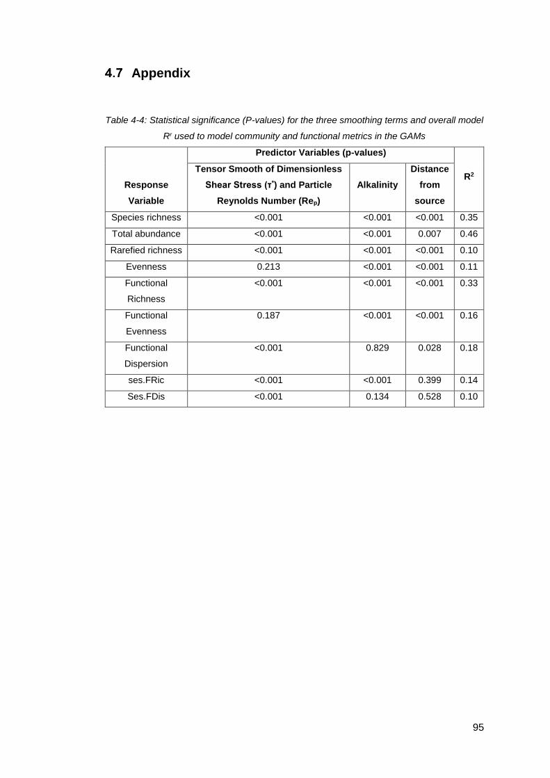
95

Appendix

Table 4-4: Statistical significance (P-values) for the three smoothing terms and overall model

Rr used to model community and functional metrics in the GAMs

Response

Variable

Predictor Variables (p-values)

R2 Tensor Smooth of Dimensionless

Shear Stress (τ*) and Particle

Reynolds Number (Rep)

Alkalinity

Distance

from

source

Species richness <0.001 <0.001 <0.001 0.35

Total abundance <0.001 <0.001 0.007 0.46

Rarefied richness <0.001 <0.001 <0.001 0.10

Evenness 0.213 <0.001 <0.001 0.11

Functional

Richness

<0.001 <0.001 <0.001 0.33

Functional

Evenness

0.187 <0.001 <0.001 0.16

Functional

Dispersion

<0.001 0.829 0.028 0.18

ses.FRic <0.001 <0.001 0.399 0.14

Ses.FDis <0.001 0.134 0.528 0.10

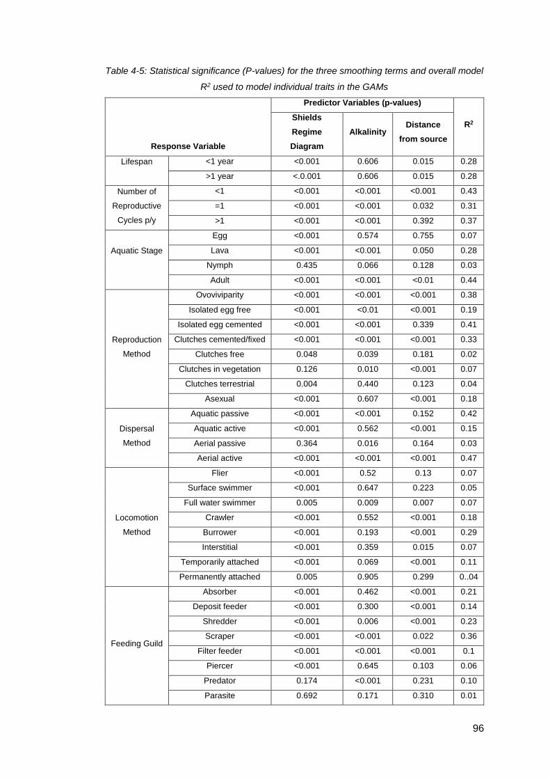
96

Table 4-5: Statistical significance (P-values) for the three smoothing terms and overall model

R2 used to model individual traits in the GAMs

Response Variable

Predictor Variables (p-values)

R2 Shields

Regime

Diagram

Alkalinity Distance

from source

Lifespan

<1 year <0.001 0.606 0.015 0.28

>1 year <.0.001 0.606 0.015 0.28

Number of

Reproductive

Cycles p/y

<1 <0.001 <0.001 <0.001 0.43

=1 <0.001 <0.001 0.032 0.31

>1 <0.001 <0.001 0.392 0.37

Aquatic Stage

Egg <0.001 0.574 0.755 0.07

Lava <0.001 <0.001 0.050 0.28

Nymph 0.435 0.066 0.128 0.03

Adult <0.001 <0.001 <0.01 0.44

Reproduction

Method

Ovoviviparity <0.001 <0.001 <0.001 0.38

Isolated egg free <0.001 <0.01 <0.001 0.19

Isolated egg cemented <0.001 <0.001 0.339 0.41

Clutches cemented/fixed <0.001 <0.001 <0.001 0.33

Clutches free 0.048 0.039 0.181 0.02

Clutches in vegetation 0.126 0.010 <0.001 0.07

Clutches terrestrial 0.004 0.440 0.123 0.04

Asexual <0.001 0.607 <0.001 0.18

Dispersal

Method

Aquatic passive <0.001 <0.001 0.152 0.42

Aquatic active <0.001 0.562 <0.001 0.15

Aerial passive 0.364 0.016 0.164 0.03

Aerial active <0.001 <0.001 <0.001 0.47

Locomotion

Method

Flier <0.001 0.52 0.13 0.07

Surface swimmer <0.001 0.647 0.223 0.05

Full water swimmer 0.005 0.009 0.007 0.07

Crawler <0.001 0.552 <0.001 0.18

Burrower <0.001 0.193 <0.001 0.29

Interstitial <0.001 0.359 0.015 0.07

Temporarily attached <0.001 0.069 <0.001 0.11

Permanently attached 0.005 0.905 0.299 0..04

Feeding Guild

Absorber <0.001 0.462 <0.001 0.21

Deposit feeder <0.001 0.300 <0.001 0.14

Shredder <0.001 0.006 <0.001 0.23

Scraper <0.001 <0.001 0.022 0.36

Filter feeder <0.001 <0.001 <0.001 0.1

Piercer <0.001 0.645 0.103 0.06

Predator 0.174 <0.001 0.231 0.10

Parasite 0.692 0.171 0.310 0.01

97

5 Benthic invertebrate response to riverbed

disturbance

Abstract

Riverbed disturbance, induced by the spatio-temporal variability of river flow, is known

to be a primary control on habitat structure and physical diversity in fluvial systems.

However, studies across large spatial scales and over multi-year time periods are

rare. This study aimed to address this shortfall by quantifying the response of

macroinvertebrate communities to riverbed disturbances at a national scale. Using a

composite dataset of 118 locations based on annual monitoring data, I modelled

community richness, persistence among years and the proportion of resistance and

resilience traits using variables describing the riverbed disturbance regime and water

quality. Evidence for a response to disturbance was limited to an increase in

community persistence with greater disturbance: the other major result was a water

quality signal that may have masked further community responses to physical habitat.

As an initial step towards linking geomorphological disturbance and community

composition through time, this study has shown that future efforts need to include

small-scale experimental studies that are capable of accounting for water quality

drivers, alongside such national-scale analyses, in order to isolate the response to

physical disturbance.

98

Introduction

Disturbance has a key role in structuring ecological communities, and occurs both

naturally and as a result of human actions (Connell, 1978; Sousa, 1984; Hobbs and

Huenneke, 1992). It acts to change the state of an ecological community via chemical,

biological or physical mechanisms, and can induce a response at all scales within an

ecosystem (Resh et al., 1998; Lake, 2000). Classic ecological theory predicts that

intermediate levels of disturbance may maximise species diversity, with inter-specific

competition restricting diversity at lower disturbance and harsh environmental

conditions limiting diversity at high disturbance levels (Connell, 1978; Townsend et

al., 1997), although empirical evidence suggests that the relationship with disturbance

is more complex (e.g. Mackey and Currie, 2001; Fox, 2013). Strikingly, there is strong

evidence for a consistent response amongst species’ ecological traits to more

frequent or intense disturbance across ecosystems, with studies in terrestrial, aquatic

and marine environments all showing evidence for increases in the prevalence of

traits associated with resisting disturbance or rapid recovery following disturbance i.e.

resistance or resilience traits (e.g. Townsend et al., 1997; Ding et al., 2012; Vinagre

et al., 2017; Chapter 4). As ecosystems come under ever greater pressure from

external factors such as climate change and urbanisation (Barker et al., 2016;

Ummenhofer and Meehel, 2017), their response to and recovery from disturbance

becomes of greater importance (Mouillot et al., 2013; Graham et al., 2015). Here, I

aim to quantify the impact of riverbed disturbance by high flows on macroinvertebrate

communities at a national scale and over a 20-year time period.

In freshwaters, disturbance is manifested as a change in the chemical, physical or

biological environment that has the potential to kill or displace organisms, deplete

resources such as food, and degrade or destroy habitat structure (Resh et al., 1988;

Lake, 2000). These may be in the form of discrete ‘pulse’ events, such as floods, or

prolonged ‘press’ or ‘ramp’ disturbances, such as channelization or the impacts of

changing catchment land use (Lake, 2000). Biological disturbances include the

introduction of non-native, invasive taxa, which can spread virulently and rapidly

overwhelm native taxa (Kelly et al., 2003). Chemically-induced disturbances are often

the result of wider physical or biological changes within the catchment, such as

greater nutrient levels leading to eutrophication and reduced dissolved oxygen levels

(Gulis et al., 2006) or afforestation with conifers reducing soil buffering to acid rainfall,

leading to lower stream pH (Weatherly and Ormerod, 1987; Collier et al., 1989), as

well as direct pollution events (Johnson and Finley, 1980; Mason, 2002). The close

99

relationship between invertebrate communities and water quality induced disturbance

has seen invertebrates used as a proxy for water quality in the UK (Metcalfe, 1989).

The strength of the water quality signal is likely to mask subtler relationships between

invertebrate communities and other disturbance gradients. Improvements in water

quality in recent decades have allowed a recovery in invertebrate diversity (Vaughan

and Ormerod, 2014), which may de-couple this relationship in some instances. Here,

I use long-term monitoring data to study the temporal component of physical

disturbance, extending beyond previous studies which have typically used space for

time substitutions or short-term before/after comparisons. I also consider the

relationship between improving water quality and invertebrate community resistance

or resilience to physical disturbance, hypothesising that the increased community

diversity will enable invertebrates to better withstand physical disturbance events.

Physical disturbances in freshwater environments principally involve changes in

water or sediment (i.e. physical habitat) availability (Lake, 2000). Periods of drought

can directly affect freshwater communities by reducing or eliminating suitable habitat

and fragmenting stream continuity (Hynes, 1958; Extence, 1981; Bonada et al.,

2006), and can also exacerbate pressures such as salinity, water temperature, low

dissolved oxygen and resource competition (Larimore et al., 1959; Power et al., 1985;

Gutierrez-Canovas et al. 2015). Catchment land use practices (e.g. intensive

agriculture) and local bank erosion (e.g. cattle poaching) can result in excessive

inputs of fine sediment into watercourses, causing burial of existing habitat and low

near-bed dissolved oxygen levels (Sear, 1993; Larsen and Ormerod, 2010), whilst

the removal of riparian vegetation reduces channel shading, leading to increased

water temperatures (Quinn et al., 1992). Floods increase the flow velocity in a

watercourse, therefore increasing the shear stress imparted on the river channel and

any organisms which reside in, on or under the riverbed (Bathurst et al., 1979). This

increased shear stress can directly or indirectly disturb organisms by forcibly

removing them from their habitat (i.e. sediment) or by moving them and their habitat

in combination (Gibbins et al., 2007). Floods can also cause indirect disturbance by

removing food (e.g. periphyton) from the riverbed (Bond and Downes, 2000; Death,

2002), or by changing channel morphology (i.e. physical habitat) and the provision of

refugia (Flecker and Feifarek, 1994). They are a classic example of a pulse

disturbance, with a short-term, discrete event often having major effects on river

ecosystems through multiple mechanisms (Woodward et al., 2016).

100

The severity of a flood can be split into three components: magnitude, frequency and

timing, which could affect riverine communities in different ways (Olden and Poff,

2003). Future changes in land use and climate are predicted to exacerbate flood flows

and sediment transport in the UK (Hannaford and Marsh, 2006). Evidence suggests

that climate change forcing is already underway (Pall et al., 2011), although it is

difficult to attribute individual flood events to these drivers (Robson, 2002; Stevens et

al., 2016). It is often assumed that both the frequency and magnitude of flood events

will increase in the future (particularly in the UK) but current evidence suggests that

only flood frequency and timing are changing (Mallakpour and Villarini, 2015; Bloschl

et al., 2017; Wasko and Sharma, 2017). Larger and/or more frequent floods are

expected to result, at least initially, in more frequent and dramatic bed disturbances

until channel morphology is modified to convey this change in flow regime, either by

increasing bed armouring or increasing channel width (Goudie, 2006). The impact of

these flow regime changes on invertebrate communities is currently unclear, but it is

well known that communities are sensitive to inter-annual variations in climate (e.g.

Bradley and Ormerod, 2001; Clews et al., 2010), although the relative contribution of

riverbed stability to this has typically been ignored. Flood timing has been shown to

directly influence invertebrate community composition and impact upon it for multiple

subsequent seasons (Sagar, 1986; Quinn and Hickey, 1994; Lytle, 2003). Floods that

occur during vulnerable life stages of a population are more likely to result in a decline

in the population. It is therefore hypothesised that physical disturbances occurring in

summer, when many invertebrates are active in the river channel, would have a

greater impact upon community composition than disturbances that occurred in

winter, when high flows (at least in the UK) are much more common and invertebrates

are in dormant life stages.

Translating predicted changes to the flow regime into the effects on bed stability and

disturbance requires a measure of the initiation of sediment transport. In alluvial

rivers, those with riverbeds composed of loose sediment, these disturbance events

are relatively frequent, occurring on average with the same period as bankfull

discharge (Benda and Dunne, 1997b). Evidence suggests that bankfull discharge,

which in unmodified channels has a return period of approximately two years, is the

dominant discharge determining channel structure (Pickup and Warner, 1976;

Williams, 1978; Andrews, 1980; Phillips and Jerolmack, 2016). Disturbance regimes

vary through space, as catchment geology, relief and climate control flow regimes,

hydrograph steepness and sediment calibre (e.g. a steep, impermeable catchment

versus a lowland baseflow dominated catchment) and through time (Shaw et al.,

101

2011). The initiation of disturbance is taken as the point at which bed load transport

begins to occur in the channel. At this point, riverbed sediment begins to move

downstream and rapidly transitions to full mobility of the riverbed surface under

greater flows (Van Rjin, 1984). This initiation of sediment transport can be estimated

using various methods, including critical shear stress, Froude number/sediment

transport relations and critical specific stream power (see Chapter 2). Here, I chose

critical specific stream power as it has the lowest data requirements (i.e. gradient,

discharge, width and mean sediment size) and has been shown to be strongly

correlated to the onset of bed load transport (Parker et al., 2011). Bed disturbance

was defined as the point at which specific stream power exceeds the critical value.

Previous efforts to investigate the interaction between invertebrate communities and

riverbed disturbance have mainly been limited to single reach or catchment scales

due to time and data constraints (e.g. Death and Winterbourn, 1995; Townsend et al.,

1997; McCabe and Gotelli 2000; Miyake and Nakano, 2002), although some larger

scale studies have also been conducted (e.g. Kusnierz et al., 2015). They have

provided evidence that with increasing disturbance, communities become less

diverse (e.g. Death and Winterbourn, 1995) and have a greater proportion of

organisms displaying resistance or resilience traits (e.g. high mobility, small body

form, short lifespans and fast reproductive cycles; Townsend et al., 1997). More

general studies of the role of flow regime in modulating invertebrate community

structure have also been undertaken, using similar datasets to the current chapter

but over shorter time periods and with fewer locations (e.g. Wagner and Schmit, 2004;

Monk et al., 2006; 2007; 2008; Greenwood and Booker, 2015; 2016). These have

found that extremes of high and low flow correlate with predictable changes in the

invertebrate community (e.g. lotic-invertebrate index for flow evaluation (LIFE) score;

Monk et al., 2006; 2007; 2008), that flood timing can influence invertebrate

emergence (Wagner and Schmit, 2004) and that anthropogenic modifications to the

flow regime can alter the dispersal ability of aquatic insects (Greenwood and Booker,

2016). The natural next step is to make an explicit link between the hydrology,

sediment transport and mobility, and the invertebrate community.

This chapter builds on Chapter 4 by adding a temporal element to investigate

community response to bed disturbance events over a 20-year timespan. Here, I want

to understand how riverbed disturbance shapes the composition and function of

benthic invertebrate communities, and whether this relationship has changed with

improving water quality over the past 20 years (Vaughan and Ormerod, 2012; 2014).

102

Using a novel composite dataset of 118 sites with multiple years sampled (380

samples in total) from across England and Wales, including invertebrate

communities, water chemistry, geomorphology and discharge from neighbouring

monitoring locations, the relationships between riverbed disturbance and invertebrate

diversity, traits and turnover are evaluated. The following hypotheses are tested:

Invertebrate communities will be less diverse, exhibit a higher turnover of taxa

through time and have a greater proportion of resistance and/or resilience

traits where the riverbed is disturbed more regularly;

Invertebrate communities are more sensitive to bed/hydrological disturbance

in summer cf. winter; and

Recovery from poor water quality increases community resistance to bed

disturbance (i.e. there will be a smaller change in community composition

between years in response to a similar level of river bed disturbance).

103

Methods

5.3.1 Data Sources

To capture information about river flow, channel morphology, water quality and

invertebrate community composition, data were amalgamated from datasets held by

the Environment Agency (EA), Natural Resources Wales (NRW), the National River

Flow Archive (NRFA) and the Centre for Ecology and Hydrology (CEH). These

datasets are described in detail in the following sections.

5.3.2 Macroinvertebrate data

Environment Agency Monitoring data

Macroinvertebrate data for the period of 1991 to 2011 were obtained from the

Environment Agency’s biological sampling network. Macroinvertebrate samples were

collected in spring (March–May inclusive) using a standardized three-minute kick-

sampling protocol (Murray- Bligh, 1999). A quality assurance scheme ensured that

the error rate in the data remained near constant after 1990 (Vaughan and Ormerod,

2014). Data were extracted for 78 taxa, based upon the individual families and

composite family groups used in the Biological Monitoring Working Party (BMWP)

scoring system, but updated to reflect recent changes in taxonomy (Centre for

Ecology & Hydrology, 2011; Table 5-5). All data were converted to presence–absence

to avoid problems with changing taxonomy and different methods of recording

abundance.

Trait data

Based on Chapter 4, five candidate ecological traits (Table 5-1) were selected from

the invertebrate trait database of Tachet et al. (2002) to describe resistance and

resilience strategies. The selected traits have been widely used to indicate relative

resistance and resilience (e.g. Bonada et al., 2007; Larsen and Ormerod, 2010;

Doledec et al., 2011; Gutiérrez-Cánovas et al., 2015). The trait data was assigned at

the genus-level and had fuzzy-coded scores from zero to three indicating individual

trait affinity within each trait group (e.g. individual scores for each reproduction

method; Tachet et al., 2002). These were converted to percentage affinity to each

trait category to standardise for potential differences in the fuzzy-coded scores

(Gutierrez-Canovas et al., 2015). The sum of the individual categories for each trait

group was 100%.

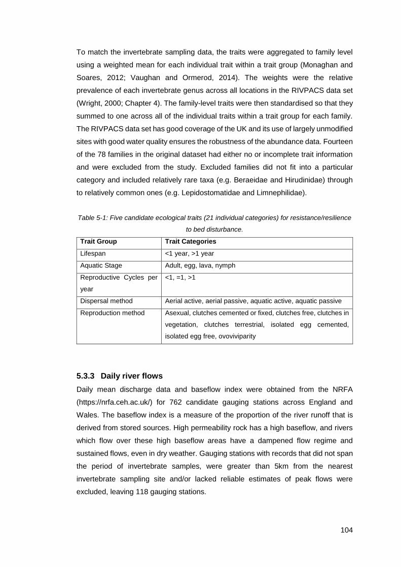
104

To match the invertebrate sampling data, the traits were aggregated to family level

using a weighted mean for each individual trait within a trait group (Monaghan and

Soares, 2012; Vaughan and Ormerod, 2014). The weights were the relative

prevalence of each invertebrate genus across all locations in the RIVPACS data set

(Wright, 2000; Chapter 4). The family-level traits were then standardised so that they

summed to one across all of the individual traits within a trait group for each family.

The RIVPACS data set has good coverage of the UK and its use of largely unmodified

sites with good water quality ensures the robustness of the abundance data. Fourteen

of the 78 families in the original dataset had either no or incomplete trait information

and were excluded from the study. Excluded families did not fit into a particular

category and included relatively rare taxa (e.g. Beraeidae and Hirudinidae) through

to relatively common ones (e.g. Lepidostomatidae and Limnephilidae).

Table 5-1: Five candidate ecological traits (21 individual categories) for resistance/resilience

to bed disturbance.

Trait Group Trait Categories

Lifespan <1 year, >1 year

Aquatic Stage Adult, egg, lava, nymph

Reproductive Cycles per

year

<1, =1, >1

Dispersal method Aerial active, aerial passive, aquatic active, aquatic passive

Reproduction method Asexual, clutches cemented or fixed, clutches free, clutches in

vegetation, clutches terrestrial, isolated egg cemented,

isolated egg free, ovoviviparity

5.3.3 Daily river flows

Daily mean discharge data and baseflow index were obtained from the NRFA

(https://nrfa.ceh.ac.uk/) for 762 candidate gauging stations across England and

Wales. The baseflow index is a measure of the proportion of the river runoff that is

derived from stored sources. High permeability rock has a high baseflow, and rivers

which flow over these high baseflow areas have a dampened flow regime and

sustained flows, even in dry weather. Gauging stations with records that did not span

the period of invertebrate samples, were greater than 5km from the nearest

invertebrate sampling site and/or lacked reliable estimates of peak flows were

excluded, leaving 118 gauging stations.

105

5.3.4 Water quality

Water quality data for 1991 to 2011 were obtained from the Environment Agency’s

water information monitoring system (WIMS). Phosphate, nitrate and biological

oxygen demand (BOD) were recorded monthly using standard methods (Standing

Committee of Analysts 1981, 1987, 1992). Median values were calculated at each

sampling site for the 12 months preceding the start of the spring invertebrate sampling

season (i.e. from March in the preceding year through to February in the current year).

Where >50% of values were below detection limits, values were estimated using the

regression on order statistics method in R’s NADA package (Lee and Helsel, 2005).

Years were excluded from each sampling site if they contained fewer than nine

monthly samples.

5.3.5 River Habitat Survey

The River Habitat Survey (RHS) was developed in 1994 to characterize the physical

character and quality of river habitats across the UK (Raven et al., 1998). It has since

been used at over 25,000 sites in the UK and elsewhere across Europe. An individual

RHS involves a survey of a 500-m length of channel with ten spot-checks that record

features at 50-m intervals and a sweep-up section that records the presence,

absence, or extensiveness (≥33% of channel length) of features within the reach

(Raven et al., 1998). Features include the type and extent of channel vegetation, any

modifications to the channel and the dominant substrate type. Finally, each RHS

location has an accompanying estimate of channel slope, measured from 1:50,000

scale maps over a 1-km length centred on the mid-point of the study reach (Raven et

al., 1998). Map-derived channel slope corresponds well with field measurements

(Montgomery et al., 1998) and is often more accurate than slope derived from digital

elevation models due to errors in channel length estimation as a result of pixel size

(Clarke et al., 2008; Fisher et al., 2013).

RHS data for channel slope and bed material (spot checks) were used in the analysis.

The bed material spot checks were converted into an average ɸ score based on

approximate values for median particle size of each size class, using a similar method

to Gurnell et al. (2010):

𝐷50 = (−8 ∗ 𝐵𝑂 − 7 ∗ 𝐶𝑂 − 3.5 ∗ 𝐺𝑃 + 1.5 ∗ 𝑆𝐴 + 6 ∗ 𝑆𝐼 + 9 ∗ 𝐶𝐿)

(𝐵𝑂 + 𝐶𝑂 + 𝐺𝑃 + 𝑆𝐴 + 𝑆𝐼 + 𝐶𝐿)

106

Where BO = boulder, CO = cobble, GP = gravel-pebble, SA = sand, SI = silt and CL

= clay. Sites were limited to those with gravel or coarser beds, in order to comply with

the channel width relation used to calculate specific stream power (Hey and Thorne,

1986), which only applies to gravel-bed rivers in the UK.

5.3.6 Site Selection

The use of four largely independent sampling schemes (invertebrates, chemistry,

RHS and flow gauging) resulted in few locations where all information was available,

but there were many occurrences where sampling sites were in close proximity.

Combining data from nearby locations is common practice in studies based on river

monitoring data (e.g. Naura and Robinson, 1998; Monk et al., 2006; 2007; 2008;

Vaughan and Ormerod, 2012; 2014) and has proven to be an effective approach for

utilising existing data sets (Vaughan and Ormerod, 2010). Potential study sites were

selected based on the following criteria:

Chemistry and RHS sites within 2km of the invertebrate sampling location,

located on the same watercourse and with no major tributaries between them

(verified by catchment area where possible, otherwise by a visual check);

A gauging station within 5km of the invertebrate sampling location, with no

major tributaries in between (where possible based on a check of upstream

catchment area, or otherwise a visual check using GIS mapping).

These distances were chosen as they represented the best trade-off between

geographic coverage and data integrity. Where multiple sites met the criteria to match

to an invertebrate sampling site, sites were selected to provide the best temporal

coverage of discharge and chemistry, and shortest distance to RHS site. Mean

distances from an invertebrate sampling site to a gauging station, water chemistry

site and RHS site were 1300m, 250m and 670m respectively.

The final data set comprised 118 regularly sampled sites (mean = nine years

sampled) across England and Wales (Figure 2). They had catchment areas of 7 –

4325 km2 and ranged from upland, high energy rivers such as the River Wye at

Erwood, mid-Wales to lowland, low-energy rivers such as the River Mimram at

Panshanger Park, Hertford.

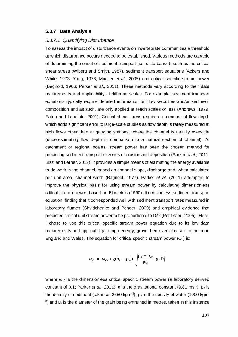
107

5.3.7 Data Analysis

5.3.7.1 Quantifying Disturbance

To assess the impact of disturbance events on invertebrate communities a threshold

at which disturbance occurs needed to be established. Various methods are capable

of determining the onset of sediment transport (i.e. disturbance), such as the critical

shear stress (Wiberg and Smith, 1987), sediment transport equations (Ackers and

White, 1973; Yang, 1976; Mueller et al., 2005) and critical specific stream power

(Bagnold, 1966; Parker et al., 2011). These methods vary according to their data

requirements and applicability at different scales. For example, sediment transport

equations typically require detailed information on flow velocities and/or sediment

composition and as such, are only applied at reach scales or less (Andrews, 1979;

Eaton and Lapointe, 2001). Critical shear stress requires a measure of flow depth

which adds significant error to large-scale studies as flow depth is rarely measured at

high flows other than at gauging stations, where the channel is usually overwide

(underestimating flow depth in comparison to a natural section of channel). At

catchment or regional scales, stream power has been the chosen method for

predicting sediment transport or zones of erosion and deposition (Parker et al., 2011;

Bizzi and Lerner, 2012). It provides a simple means of estimating the energy available

to do work in the channel, based on channel slope, discharge and, when calculated

per unit area, channel width (Bagnold, 1977). Parker et al. (2011) attempted to

improve the physical basis for using stream power by calculating dimensionless

critical stream power, based on Einstein’s (1950) dimensionless sediment transport

equation, finding that it corresponded well with sediment transport rates measured in

laboratory flumes (Shvidchenko and Pender, 2000) and empirical evidence that

predicted critical unit stream power to be proportional to Di1.5 (Petit et al., 2005). Here,

I chose to use this critical specific stream power equation due to its low data

requirements and applicability to high-energy, gravel-bed rivers that are common in

England and Wales. The equation for critical specific stream power (ωc) is:

ωc = ω𝑐∗ ∗ g(ρs − ρw). √ρs − ρw

ρw . g . Di

3

where ωc* is the dimensionless critical specific stream power (a laboratory derived

constant of 0.1; Parker et al., 2011), g is the gravitational constant (9.81 ms-1), ps is

the density of sediment (taken as 2650 kgm-3), pw is the density of water (1000 kgm-

3) and Di is the diameter of the grain being entrained in metres, taken in this instance

108

as the D50 calculated in Section 5.3.5. A disturbance was deemed to have occurred

when the critical specific stream power was exceeded by the specific stream power.

Specific stream power, the rate of energy expenditure per channel length, normalised

by channel width, was defined as:

𝜔 = 𝜌𝑔𝑄𝑆

𝑤

Where ρw is equal to the density of water (taken as 1000 kg m-3), g is equal to the

gravitational constant (taken as 9.81 m s-1), Q is equal to discharge (m3 s-1), taken as

the daily flow from 1990-2013 for each site, S is equal to average bed slope (m m-1)

as contained in the RHS data, and w is channel width in metres. Channel width (w)

was estimated from the discharge using Hey and Thorne’s (1986) equation from

Knighton’s (1999) study on gravel-bed rivers in the UK:

𝑤 = 3.42 𝑄0.46

Once the daily specific stream power was calculated for each of the 118 gauging

stations, riverbed disturbance was identified as periods where the critical specific

stream power (Parker et al., 2011) was exceeded by the daily specific stream power.

This daily specific stream power was likely to be a conservative estimate of when

disturbance had occurred as average daily discharge is not the peak discharge of an

event (Fill and Steiner, 2003).

To capture the frequency, magnitude and duration of disturbance at each site, the

following metrics were calculated over the 12 months preceding an invertebrate

sample:

1. Number of days when the riverbed was disturbed. A cumulative total of the

annual number of days where the specific stream power exceeded the critical

specific stream power;

2. The cumulative intensity of disturbance. A measure of the cumulative

exceedance (daily exceedance = SSP / Critical SSP) above the critical

threshold over the past year;

3. The peak intensity of disturbance. The largest daily event with the value

recorded as a multiple that the critical power was exceeded by (i.e. SSP /

Critical SSP); and

109

4. The number of discrete disturbance events. Events were counted as discrete

if separated by at least 2 days where the critical threshold was not exceeded

to ensure single storm events were only counted as one event.

Based upon work using related hydrological indices (Olden and Poff, 2003), it was

expected that the disturbance metrics would display multicollinearity. A principal

component analysis (PCA) was used to identify the relationships between them and

provide a simplified disturbance index (PC1) for use in subsequent analyses (see

Results for details of the PCA). To address Hypothesis 2 (summer vs. winter

disturbance) the metrics were re-run for March to August (Summer) and September

to February (Winter) only. These were then ordinated using the same PCA procedure,

and seasonal PC1 scores estimated to indicate the disturbance regime at each site

for summer or winter only.

5.3.7.2 Invertebrate community structure

The response of invertebrate community structure to riverbed disturbance was

assessed using two metrics: i) taxon richness; and ii) Jaccard dissimilarity index

between consecutive years. Taxon richness was simply a count of the number of

families present for each sample. The Jaccard index (Jaccard, 1908) was selected to

describe the dissimilarity between samples (in this case two invertebrate

communities) as it is an established measure of persistence that has been used in

several river studies (e.g. Milner et al., 2006; Collier, 2008). The index was calculated

using the vegdist function in the vegan R package (Oksanen et al., 2017). This

provided a measure of the dissimilarity in the composition between the communities

in consecutive years, with a value of zero indicating that an identical set of families

was present in both samples, and a value of one indicating that the two samples had

no families in common.

5.3.7.3 Trait representation

An ordination analysis was used to provide a simple overview of how the prevalence

of potential resistance and resilience traits varied among invertebrate communities.

The aim was to provide a simplified representation of trait variation among

communities for use in subsequent analysis (cf. analysis of individual traits; Chapter

4). The 877 invertebrate samples (across 118 sites) were ordinated on the five groups

of candidate resistance and resilience traits (18 individual trait categories) using fuzzy

correspondence analysis (Usseglio-Polatera et al., 2000; ade4 R package). The first

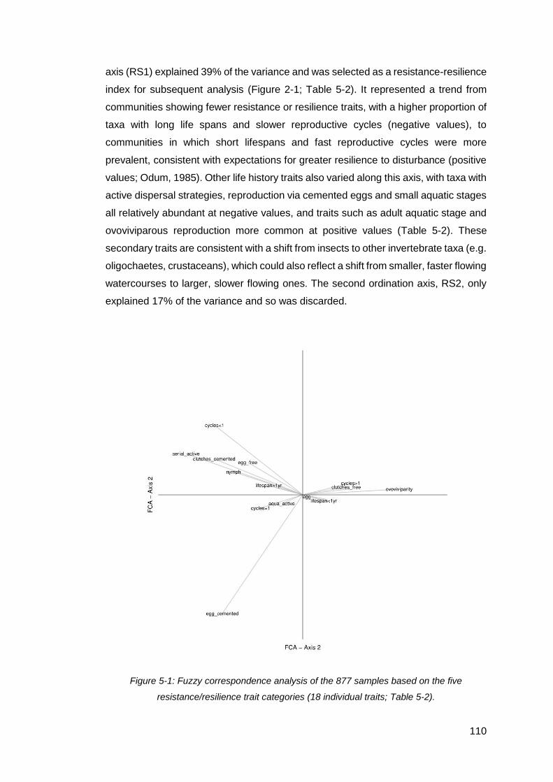
110

axis (RS1) explained 39% of the variance and was selected as a resistance-resilience

index for subsequent analysis (Figure 2-1; Table 5-2). It represented a trend from

communities showing fewer resistance or resilience traits, with a higher proportion of

taxa with long life spans and slower reproductive cycles (negative values), to

communities in which short lifespans and fast reproductive cycles were more

prevalent, consistent with expectations for greater resilience to disturbance (positive

values; Odum, 1985). Other life history traits also varied along this axis, with taxa with

active dispersal strategies, reproduction via cemented eggs and small aquatic stages

all relatively abundant at negative values, and traits such as adult aquatic stage and

ovoviviparous reproduction more common at positive values (Table 5-2). These

secondary traits are consistent with a shift from insects to other invertebrate taxa (e.g.

oligochaetes, crustaceans), which could also reflect a shift from smaller, faster flowing

watercourses to larger, slower flowing ones. The second ordination axis, RS2, only

explained 17% of the variance and so was discarded.

Figure 5-1: Fuzzy correspondence analysis of the 877 samples based on the five

resistance/resilience trait categories (18 individual traits; Table 5-2).

111

Table 5-2: Loading coefficients for the first two axes of a fuzzy correspondence analysis

conducted on the five resistance/resilience trait categories (18 individual traits). Three

reproduction categories (asexual, terrestrial, in vegetation) were excluded due to low

proportions skewing the FCA.

Traits CS1 CS2

Lifespan <1 year 0.41 -0.24

>1 year -0.66 0.39

Reproductive Cycles per year <1 -1.70 2.83

=1 -0.81 -0.54

>1 0.92 0.48

Aquatic Stage Egg 0.08 -0.08

Lava -0.55 0.31

Nymph -1.33 0.94

Adult 0.48 -0.25

Reproduction Method Ovoviviparity 1.86 0.23

Isolated eggs free -1.06 1.32

Isolated egg cemented -1.55 -4.84

Clutches cemented or fixed -1.71 1.46

Clutches free 0.84 0.32

Dispersal Method Aquatic passive 0.45 -0.18

Aquatic active -0.41 -0.36

Aerial passive 0.91 0.24

Aerial active -2.25 1.68

5.3.7.4 Regression Models

Two different approaches to regression analysis were used to test the hypotheses: i)

a cross-sectional approach, focusing on among-site differences in the invertebrate

community at two time points, and ii) a longitudinal approach using the complete 21-

year data set. Overall richness, the Jaccard index between years (persistence) and

the index of resistance-resilience traits (RS1) were analysed in each case. For the

first approach, the mean values of the three invertebrate variables at each sample

site were regressed against the mean value of the site’s disturbance index (PC1)

using simple linear models (to address hypothesis 1). Phosphate, BOD, nitrate and

temperature were also included in the models to control for variation among sites.

Phosphate and BOD were log transformed and the fit of the models checked using

plots of the residuals. To minimise the potential confounding effect of improving water

112

quality over the study period (Parr and Mason, 2003; Vaughan et al., 2012; 2014),

the analysis was repeated at two different 5-year periods, one early (1993-1998) and

one late (2003-2008) in the study period (cf. averaging across the complete 21-year

period). If the results were similar at both time periods it would provide evidence that

any disturbance relationship was not altered by changing water quality.

The second approach modelled the three invertebrate variables for each sample site

as a function of the disturbance index (PC1) and the first axis of a PCA of the water

quality variables. The latter was run with phosphate, BOD and nitrate, and the first

principal component explained 64% of the variance. Negative values of the

component represented high water quality i.e. low concentrations of nitrate and

phosphate, and low BOD. Water quality was summarised in this way to simplify the

model and minimise potential convergence problems (e.g. due to collinearity).

Generalised additive mixed models (GAMMs), using R’s mgcv package, were used

to relate the invertebrate data to disturbance and water quality, with identity links and

Gaussian errors. Site was included as a random term in the model to account for

multiple observations being taken from the same locations (through time). The

disturbance and water quality PCA axes were modelled using a tensor product of thin-

plate regression splines, with the degree of smoothing determined by generalized

cross validation, which allows potential interactions between them to be modelled

(Wood, 2006; see also Chapter 3). The fit of each model was checked by examining

plots of the residuals. This approach was used to: (1) investigate whether there was

a difference in response to summer vs. winter disturbance (hypothesis 2), by fitting

the models twice, using disturbance PC1 for summer or winter, and (2) indicate

whether the three response variables changed with improving water quality

(hypothesis 3). To examine the effect of changing water quality on the relationships

between invertebrates and disturbance, model predictions were generated with

changing disturbance at both good and poor water quality. In the absence of other

obvious values, ‘good’ and ‘poor’ were taken as the 25th and 75th percentiles of the

water quality PCA axis (Harrell, 2001).

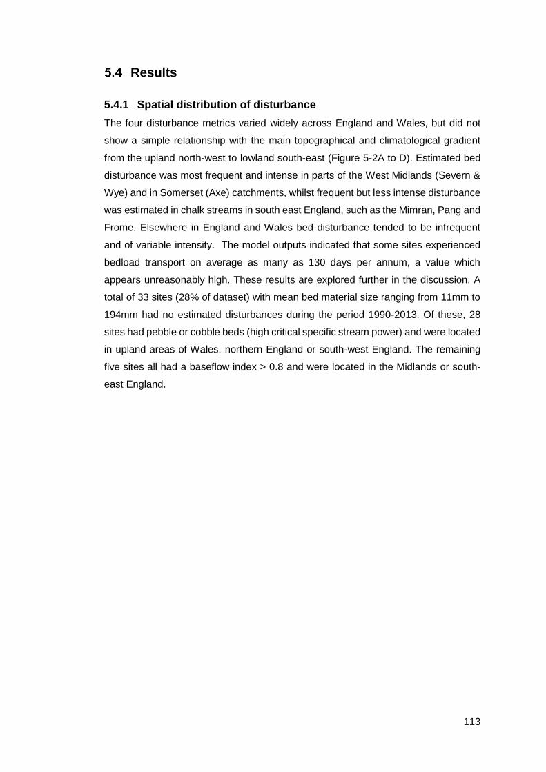
113

Results

5.4.1 Spatial distribution of disturbance

The four disturbance metrics varied widely across England and Wales, but did not

show a simple relationship with the main topographical and climatological gradient

from the upland north-west to lowland south-east (Figure 5-2A to D). Estimated bed

disturbance was most frequent and intense in parts of the West Midlands (Severn &

Wye) and in Somerset (Axe) catchments, whilst frequent but less intense disturbance

was estimated in chalk streams in south east England, such as the Mimran, Pang and

Frome. Elsewhere in England and Wales bed disturbance tended to be infrequent

and of variable intensity. The model outputs indicated that some sites experienced

bedload transport on average as many as 130 days per annum, a value which

appears unreasonably high. These results are explored further in the discussion. A

total of 33 sites (28% of dataset) with mean bed material size ranging from 11mm to

194mm had no estimated disturbances during the period 1990-2013. Of these, 28

sites had pebble or cobble beds (high critical specific stream power) and were located

in upland areas of Wales, northern England or south-west England. The remaining

five sites all had a baseflow index > 0.8 and were located in the Midlands or south-

east England.

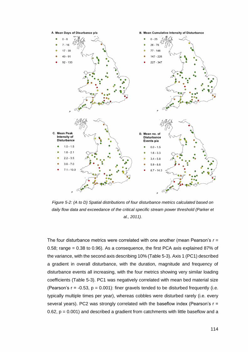
114

Figure 5-2: (A to D) Spatial distributions of four disturbance metrics calculated based on

daily flow data and exceedance of the critical specific stream power threshold (Parker et

al., 2011).

The four disturbance metrics were correlated with one another (mean Pearson’s r =

0.58; range = 0.38 to 0.96). As a consequence, the first PCA axis explained 87% of

the variance, with the second axis describing 10% (Table 5-3). Axis 1 (PC1) described

a gradient in overall disturbance, with the duration, magnitude and frequency of

disturbance events all increasing, with the four metrics showing very similar loading

coefficients (Table 5-3). PC1 was negatively correlated with mean bed material size

(Pearson’s r = -0.53, p = 0.001): finer gravels tended to be disturbed frequently (i.e.

typically multiple times per year), whereas cobbles were disturbed rarely (i.e. every

several years). PC2 was strongly correlated with the baseflow index (Pearson’s r =

0.62, p = 0.001) and described a gradient from catchments with little baseflow and a

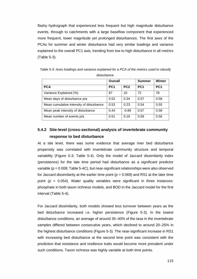
115

flashy hydrograph that experienced less frequent but high magnitude disturbance

events, through to catchments with a large baseflow component that experienced

more frequent, lower magnitude yet prolonged disturbances. The first axes of the

PCAs for summer and winter disturbance had very similar loadings and variance

explained to the overall PC1 axis, trending from low to high disturbance in all metrics

(Table 5-3).

Table 5-3: Axes loadings and variance explained for a PCA of the metrics used to classify

disturbance.

Overall Summer Winter

PCA PC1 PC2 PC1 PC1

Variance Explained (%) 87 10 72 78

Mean days of disturbance p/a 0.52 0.34 0.57 0.58

Mean cumulative intensity of disturbance 0.53 0.23 0.54 0.55

Mean peak intensity of disturbance 0.44 -0.89 0.57 0.58

Mean number of events p/a 0.51 0.19 0.59 0.56

5.4.2 Site-level (cross-sectional) analysis of invertebrate community

response to bed disturbance

At a site level, there was some evidence that average river bed disturbance

propensity was correlated with invertebrate community structure and temporal

variability (Figure 5-3; Table 5-4). Only the model of Jaccard dissimilarity index

(persistence) for the late time period had disturbance as a significant predictor

variable (p = 0.008; Table 5-4C), but near-significant relationships were also observed

for Jaccard dissimilarity at the earlier time point (p = 0.069) and RS1 at the later time

point (p = 0.054). Water quality variables were significant in three instances:

phosphate in both taxon richness models, and BOD in the Jaccard model for the first

interval (Table 5-4).

For Jaccard dissimilarity, both models showed less turnover between years as the

bed disturbance increased i.e. higher persistence (Figure 5-3). In the lowest

disturbance conditions, an average of around 35–40% of the taxa in the invertebrate

samples differed between consecutive years, which declined to around 20–25% in

the highest disturbance conditions (Figure 5-3). The near-significant increase in RS1

with increasing bed disturbance at the second time point was consistent with the

prediction that resistance and resilience traits would become more prevalent under

such conditions. Taxon richness was highly variable at both time points.

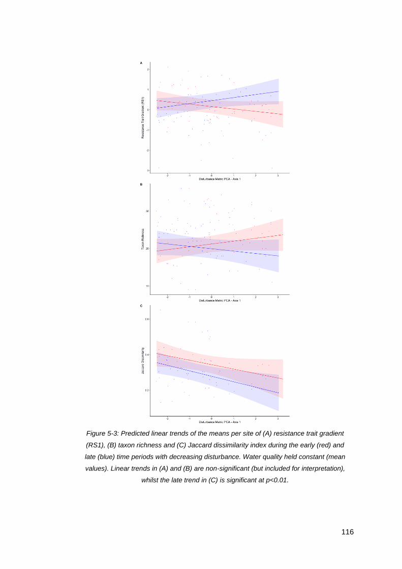
116

Figure 5-3: Predicted linear trends of the means per site of (A) resistance trait gradient

(RS1), (B) taxon richness and (C) Jaccard dissimilarity index during the early (red) and

late (blue) time periods with decreasing disturbance. Water quality held constant (mean

values). Linear trends in (A) and (B) are non-significant (but included for interpretation),

whilst the late trend in (C) is significant at p<0.01.

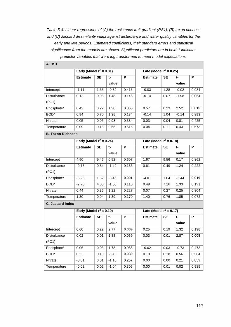
117

Table 5-4: Linear regressions of (A) the resistance trait gradient (RS1), (B) taxon richness

and (C) Jaccard dissimilarity index against disturbance and water quality variables for the

early and late periods. Estimated coefficients, their standard errors and statistical

significance from the models are shown. Significant predictors are in bold. * indicates

predictor variables that were log transformed to meet model expectations.

A. RS1

Early (Model r2 = 0.31) Late (Model r2 = 0.25)

Estimate SE t-

value

P Estimate SE t-

value

P

Intercept -1.11 1.35 -0.82 0.415 -0.03 1.28 -0.02 0.984

Disturbance

(PC1)

0.12 0.08 1.48 0.146 -0.14 0.07 -1.98 0.054

Phosphate* 0.42 0.22 1.90 0.063 0.57 0.23 2.52 0.015

BOD* 0.94 0.70 1.35 0.184 -0.14 1.04 -0.14 0.893

Nitrate 0.05 0.05 0.98 0.334 0.03 0.04 0.81 0.425

Temperature 0.09 0.13 0.65 0.516 0.04 0.11 0.43 0.673

B. Taxon Richness

Early (Model r2 = 0.24) Late (Model r2 = 0.18)

Estimate SE t-

value

P Estimate SE t-

value

P

Intercept 4.90 9.46 0.52 0.607 1.67 9.56 0.17 0.862

Disturbance

(PC1)

-0.76 0.54 -1.42 0.163 0.61 0.49 1.24 0.222

Phosphate* -5.26 1.52 -3.46 0.001 -4.01 1.64 -2.44 0.019

BOD* -7.78 4.85 -1.60 0.115 9.49 7.16 1.33 0.191

Nitrate 0.44 0.36 1.22 0.227 0.07 0.27 0.25 0.804

Temperature 1.30 0.94 1.39 0.170 1.40 0.76 1.85 0.072

C. Jaccard Index

Early (Model r2 = 0.19) Late (Model r2 = 0.17)

Estimate SE t-

value

P Estimate SE t-

value

P

Intercept 0.60 0.22 2.77 0.009 0.25 0.19 1.32 0.198

Disturbance

(PC1)

0.02 0.01 1.88 0.069 0.03 0.01 2.87 0.008

Phosphate* 0.06 0.03 1.78 0.085 -0.02 0.03 -0.73 0.473

BOD* 0.22 0.10 2.28 0.030 0.10 0.18 0.56 0.584

Nitrate -0.01 0.01 -1.16 0.257 0.00 0.00 0.21 0.839

Temperature -0.02 0.02 -1.04 0.306 0.00 0.01 0.02 0.985

118

5.4.3 Longitudinal analysis 1: The role of disturbance in summer

versus winter

There was no evidence of a stronger response to disturbance in summer over winter

for resistance traits or the Jaccard Index (Figure 5-4). The models of richness failed

to converge and were excluded. Resistance traits (RS1) models for summer (p

<0.001, r2 = 0.22) and winter (p = 0.001, r2 = 0.17) disturbance both showed that

resistance traits became more common as disturbance increased (Figure 5-4A; B),

corresponding with the results of the linear models. The response of RS1 to

increasing winter disturbance was non-linear and showed resistance traits initially

increasing, then falling and then increasing again at peak levels of disturbance (Figure

5-4B), whilst in summer resistance traits increased linearly with disturbance (Figure

5-4A). The Jaccard dissimilarity index declined with increasing disturbance in both

summer (p = 0.434, r2 = 0.01) and winter (p = 0.004, r2 = 0.10), although the predictor

smooth in summer was non-significant. The decline was steeper in winter, 33% to

27% dissimilarity, than in summer, 30% to 29%, and was consistent with the trend of

the linear models.

119

Figure 5-4: GAMM predictions for trends in resistance trait gradient (RS1) versus (A)

summer and (B) winter disturbance, and Jaccard dissimilarity index versus (A) summer

and (B) winter disturbance. Random effects are set to zero.

5.4.4 Longitudinal analysis 2: Interaction between water quality

improvements and disturbance

Resistance traits (RS1; p = 0.003, r2 = 0.15), richness (p = 0.017, r2 = 0.10) and

persistence (Jaccard dissimilarity; p = 0.003, r2 = 0.10) were all related significantly

to bed disturbance and improving water quality. Richness marginally increased with

greater disturbance in poor water quality (by c. 1.5 families) but stabilised across the

disturbance gradient with good water quality (Figure 5-5A). Resistance-resilience

traits (RS1) responded differently to bed disturbance depending upon the prevailing

water quality (Figure 5-5B). In poor water quality resistance-resilience traits became

more prevalent with increasing disturbance, whilst in good water quality they became

less prevalent (Figure 5-5B). In good water quality, Jaccard dissimilarity decreased

from approximately 33% to 30% of taxa across the disturbance gradient, whilst the

decline with increasing disturbance in poor water quality was steeper, from 34% to

28% of taxa (Figure 5-5C): similar responses to those of the site-average models.

120

Figure 5-5: GAMM predictions for trends in (A) resistance trait gradient (RS1), (B) taxon

richness and (C) Jaccard dissimilarity index for good (red) and poor (blue) water quality

with increasing disturbance (x axis). Random effects are set to zero.

121

Discussion

Evidence for the role of riverbed disturbance in altering invertebrate community

composition and function is restricted to a small number of studies (e.g. Death and

Winterbourn, 1995; Townsend et al., 1997; McCabe and Gotelli 2000; Miyake and

Nakano, 2002). These few studies, coupled with theoretical work on disturbance,

suggests that bed stability could play an important role, and so a better understanding

of this relationship is important if we are to make reliable predictions of future change

to river ecosystems. Previous studies have for good reason focussed on the impacts

of water quality (e.g. Vaughan and Ormerod, 2012; 2014) and it is only with

improvements in water quality that the influence of physical modifications and channel

change have become apparent (Newson and Newson, 2000). This study has

investigated whether there is a riverbed disturbance signal in long-term ecological

monitoring data using a novel composite dataset spanning England and Wales. The

critical specific stream power equation (Ferguson, 2005; Petit et al., 2005; Parker et

al., 2011) was selected as the threshold for disturbance due to its low data

requirements and applicability to gravel-bed rivers, which are common in Britain.

Despite the limitations of stream power in comparison to more detailed methods of

predicting the onset of sediment transport (Gomez and Church, 1989; Ferguson,

2005), this approach represents a first step towards linking process-based,

geomorphic theory with changes in the composition and function of invertebrate

communities through time and at a national scale. The following section will discuss

the limitations of the study before moving on to discuss the findings.

5.5.1 Limitations

The approach used here has four major limitations. Firstly, despite this approach

involving largely unmatched spatial and temporal coverage, the use of a composite

dataset that is applied in a manner different from its intended original use presents a

series of limitations (Vaughan and Ormerod, 2010). Despite efforts to ensure that

paired sites were in a similar location and considered river reaches with the same

ecological, physical and chemical characteristics, the distribution of ecological

communities and physical forms are known to vary at small spatial scales (Downes

et al., 1993; Poff, 1997; Benda et al., 2004). Also, in a similar vein to the previous

chapter, the available geomorphological data were particularly weak (e.g. simplistic

channel substrate measures). Although bed material size could be estimated from the

descriptive data in RHS, a quantitative measure of sediment size would have provided

greater accuracy. Other shortcomings in the use of secondary data were (1) the lack

122

of resolution in the family-level invertebrate data, potentially limiting the identification

of patterns (i.e. divergent species’ responses within a family could go unnoticed; Melo,

2005), and (2) incomplete trait information, leading to a potential bias towards well-

studied taxa (Tyler et al., 2012) – the analysis here had to exclude 14 taxa (18%) due

to lack of trait information.

The second limitation was that the threshold at which movement of sediment in the

riverbed is considered to represent a disturbance to benthic invertebrates is poorly

understood (Schwendel et al., 2010a; 2010b). Variations in the threshold of sediment

transport, due to bed armouring (Gomez, 1983), fixed objects in the channel (e,g.

large wood; Gurnell et al., 2002) or biotic influences (e.g. biofilms; Stone et al., 2008;

2011 or channel vegetation; Murray and Paola, 2003), introduces a high degree of

uncertainty in predicting the onset of riverbed disturbance. In this study a disturbance

to benthic invertebrates has been assumed to be represented by any movement of

particles within the riverbed, in line with previous studies (e.g. Cobb et al., 1992;

Townsend et al., 1997). Future studies should include experimentation to determine

whether this assumption is correct of if a different level of physical movement is

required to constitute a disturbance in ecological terms.

Thirdly, as floods can affect invertebrate communities in multiple ways (Naegeli et al.,

1995; Olson and Townsend, 2005), it is difficult to identify the causal mechanism,

even where a correlation between an expected stressor (e.g. bed disturbance) and

the community response is observed. The approach used here of filtering by flows

expected to have caused transport of riverbed material provides a first step towards

a test of these causal mechanisms. To gain a full understanding, a similar approach

to that used here needs to be combined with direct field observations of bed

movement, manipulative experiments and more detailed measures of how

invertebrate populations and resources change (e.g. with measures of basal food

resources or food web structure).

Finally, the background conditions of largely poor water quality across the UK and a

trend of improvement across the period of the study (Vaughan et al., 2012; 2014),

increases the complexity of invertebrate responses and potentially masks underlying

trends in community composition as a result of riverbed disturbance. The strong

correlation between poor water quality and reduced invertebrate diversity and

function (Whilm and Dorris, 1968; Lenat, 1988) presents a challenge when

interpreting results. Here, there were several instances where the ecological

123

relationships with disturbance varied according to the prevailing water quality. In

addition to these observed relationships, the extent to which poor water quality could

still be masking physical habitat effects is unknown. The changes in trait composition

with improving water quality (Figure 5-5A) suggest that it may still be playing an

ongoing role.

5.5.2 Spatial trends in disturbance

The metrics calculated here to describe the trends in sediment transport and riverbed

disturbance across England and Wales correspond well with known variations in flow

regime and river energy but do not display a simple upland lowland or north-west to

south-east gradient (Hannaford and Marsh, 2006). Disturbance regimes with a long

duration, moderate frequency and low peak intensity (Figure 5-2A; C; D),

corresponded closely with high base flow rivers (e.g. Great Stour and the Wiltshire

Avon; chalk streams in south eastern England). Conversely, active gravel-bed rivers

such as the Wye, Clwyd, Axe and Dulas, were also found to be frequently disturbed

but with higher peak intensities (Figure 5-2). This appeared to be a function of their

relatively small bed material (gravel) in comparison to their specific stream power

(>40 W m-2 at QMED), with high base flow rivers such as the Mimran, Pang and

Frome having comparable bed material but much lower specific stream powers (< 20

W m-2 at QMED). The limitations of the approach were evident in the results of

disturbance metrics, with some locations indicating that sediment transport occurred

for up to 130 days a year, which is unlikely. The transport threshold overestimated

disturbance where riverbeds were estimated to be composed of fine gravel. This was

likely due to a combination of mean bed surface grain size being underestimated and

the critical specific stream power threshold performing poorly where bedform

structure contributed to overall bed stability (Church et al., 1998). A priority for future

research should be to test the critical specific stream power threshold used here

across a range of coarse grain sizes.

The high values of all four disturbance metrics in the active, mostly upland, gravel-

bed rivers may be explained by their relatively unmodified form when compared to

the other (modified) rivers in the dataset. Visual inspection of the data revealed that

the 8% of sites with the highest disturbance PC1 scores all had RHS Habitat

Modification Index scores of 2 or less (Raven et al., 1998). Where rivers have been

modified by impoundments or for flood defence purposes, sediment supply and

floodplain connectivity are reduced (Petts, 1980; Downs and Thorne, 2000), and a

124

common geomorphic response of narrowing and deepening is evident (Church, 1995;

Simon and Rinaldi, 2006). This response increases the energy directed at the

riverbed rather than lateral channel adjustments (Lisle et al., 1993; Petit et al., 1996).

In this scenario, bed material becomes significantly larger as finer material is

transported away and not replenished (termed bed armouring), which stabilises the

channel against greater shear stress (Gomez, 1983). Although the formation of a

mobile armoured layer occurs naturally in many gravel-bed rivers, armouring can also

occur in response to a reduction in sediment supply from upstream (e.g. due to

anthropogenic modifications), forming a static armour layer, which would reduce the

frequency of riverbed disturbance relative to its natural state (Mao et al., 2011).

5.5.3 Evidence for invertebrate community response to disturbance

Overall, there was evidence for a response of the invertebrate community to

disturbance, but this appeared to interact with water quality, making interpretation of

the results more complex. The prevalence of resistance/resilience traits declined with

increasing disturbance in the early part of the time series (Figure 5-3A) and in the

longitudinal model with good water quality (Figure 5-5A), contrary to predictions, but

increased with disturbance in longitudinal models of summer or winter disturbance

and water quality (Figure 5-4A; B) and poor water quality (Figure 5-5A), consistent

with hypothesis 1. When focussing only on models with a statistically significant

interaction between disturbance and water quality as the predictor variable (only the

models of good and poor water quality), there appeared to be a recovery of insect

taxa with improving water quality (decreasing resistance traits). EPT taxa, which

make up a large proportion of the insect taxa in the dataset, are known to be highly

sensitive to pollution (Barbour et al., 1992) and their recovery with improvement water

quality could explain the trend shown in Figure 5-5A. This link between resistance

traits and water quality was supported further by the positive correlations between

RS1 and the three water quality variables, phosphate (Pearson’s r = 0.45, p = 0.001),

nitrate (Pearson’s r = 0.42, p = 0.001) and biological oxygen demand (Pearson’s r =

0.39, p = 0.001). The potential for water quality to affect RS1 is not surprising, as traits

thought to confer greater resistance and/or resilience are often generic and applicable

to multiple stressors, including physical and chemical disturbance. This can cause

problems when trying to use traits to diagnose stressors (e.g. Schuwirth et al., 2015).

Given the diverse set of locations at the national scale, and wide range in water quality

both across England and Wales, and through time, a strong water quality effect was

to be expected.

125

Taxon richness was the least sensitive metric to both disturbance and water quality.

It increased with disturbance in the early period cross-sectional model and under poor

water quality in the longitudinal model. One possible explanation for this result is the

greater degree of re-oxygenation and cooler water temperatures in faster flowing

upland locations, which were most prevalent at the upper end of the disturbance

gradient. Both of these effects can act of offset poor water quality, such as high BOD

(Verberk et al., 2016), and so might have promoted higher richness in these cases.

The Jaccard dissimilarity index consistently showed a trend of decreasing

dissimilarity with increasing disturbance across the cross sectional and longitudinal

models (Figure 5-3C; Figure 5-4C; 4D; Figure 5-5C). This indicated that the

persistence of taxa was greatest at intermediate to high levels of disturbance, a trend

noted by previous smaller-scale studies (Meffe and Minckley, 1987; Scarsbrook,

2002; Collier, 2008). Part of the explanation for this trend may be that the sites with

the highest levels of disturbance (and therefore energy to transport sediment and

create diverse physical forms) may also be the most spatially heterogeneous sites.

Spatial heterogeneity has been shown to reduce the temporal variability (i.e.

dissimilarity from year to year) in benthic invertebrate communities (Brown, 2003) by

providing refugia for organisms (Townsend and Hildrew, 1994). In addition to this

abiotic mechanism, the highest levels of disturbance are where the strongest habitat

filtering is expected to occur (Townsend and Hildrew, 1994, Venn et al., 2011),

selecting for a subset of taxa with traits that allow them to persist. The greater

resistance of the selected taxa may feed up to the community level, creating a

community with little variation in composition among years.

The results suggest that water quality still exerts significant control over invertebrate

community composition, despite the improvements in recent decades (Langford et

al., 2009; Durance and Ormerod 2009; Vaughan and Ormerod 2012, 2014).

Therefore, future studies of the interaction between riverbed disturbance and

invertebrate community composition will require a combined approach using large

scale statistical analysis and small-scale experimental study, where other controls

(e.g. water quality) can be held constant and the key processes and thresholds

related to disturbance can be isolated.

126

Conclusion

The main aim of this chapter was to investigate the response of invertebrate

communities to riverbed disturbance across spatial and temporal axes. A composite

dataset spanning a 20-year time period, containing biological, chemical, hydrological

and geomorphological data for sites across England and Wales, was combined with

a simple, stream power model of the threshold of bed load transport. The results

provide evidence for locations with greater bed disturbance showing increased

community persistence, irrespective of water quality. Other trends may be masked by

community-level response to water quality, both among-sites in the data set and over

widespread improvements in recent decades. The response to water quality

improvements has led to a reduction in resistance traits, hypothesised to be due to

the recovery of pollution sensitive insect taxa (e.g. EPT). This study represents a first

step towards linking geomorphological disturbance and community composition

through time and has found that future studies need to combine this approach with

small-scale experimental studies that are capable of isolating the response to physical

disturbance from other drivers such as water quality.

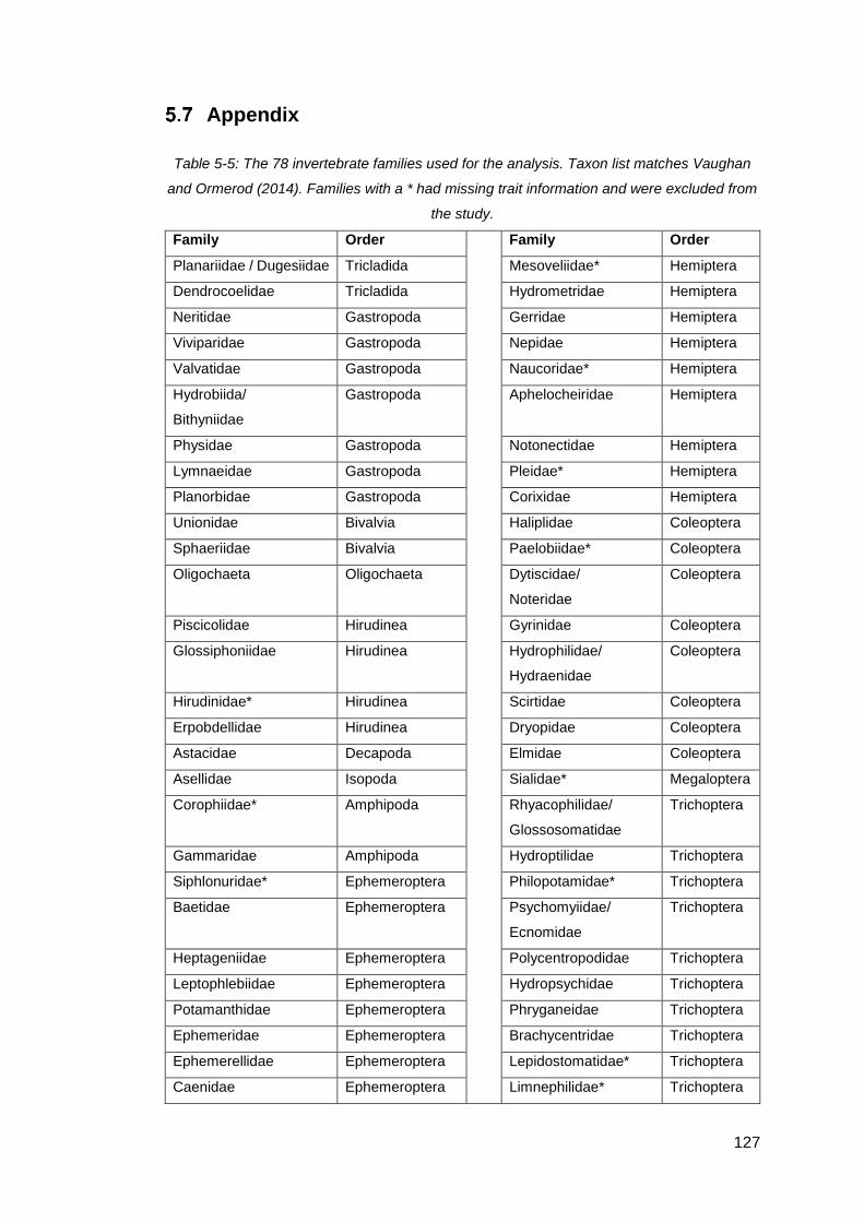
127

Appendix

Table 5-5: The 78 invertebrate families used for the analysis. Taxon list matches Vaughan

and Ormerod (2014). Families with a * had missing trait information and were excluded from

the study.

Family Order Family Order

Planariidae / Dugesiidae Tricladida Mesoveliidae* Hemiptera

Dendrocoelidae Tricladida Hydrometridae Hemiptera

Neritidae Gastropoda Gerridae Hemiptera

Viviparidae Gastropoda Nepidae Hemiptera

Valvatidae Gastropoda Naucoridae* Hemiptera

Hydrobiida/

Bithyniidae

Gastropoda Aphelocheiridae Hemiptera

Physidae Gastropoda Notonectidae Hemiptera

Lymnaeidae Gastropoda Pleidae* Hemiptera

Planorbidae Gastropoda Corixidae Hemiptera

Unionidae Bivalvia Haliplidae Coleoptera

Sphaeriidae Bivalvia Paelobiidae* Coleoptera

Oligochaeta Oligochaeta Dytiscidae/

Noteridae

Coleoptera

Piscicolidae Hirudinea Gyrinidae Coleoptera

Glossiphoniidae Hirudinea Hydrophilidae/

Hydraenidae

Coleoptera

Hirudinidae* Hirudinea Scirtidae Coleoptera

Erpobdellidae Hirudinea Dryopidae Coleoptera

Astacidae Decapoda Elmidae Coleoptera

Asellidae Isopoda Sialidae* Megaloptera

Corophiidae* Amphipoda Rhyacophilidae/

Glossosomatidae

Trichoptera

Gammaridae Amphipoda Hydroptilidae Trichoptera

Siphlonuridae* Ephemeroptera Philopotamidae* Trichoptera

Baetidae Ephemeroptera Psychomyiidae/

Ecnomidae

Trichoptera

Heptageniidae Ephemeroptera Polycentropodidae Trichoptera

Leptophlebiidae Ephemeroptera Hydropsychidae Trichoptera

Potamanthidae Ephemeroptera Phryganeidae Trichoptera

Ephemeridae Ephemeroptera Brachycentridae Trichoptera

Ephemerellidae Ephemeroptera Lepidostomatidae* Trichoptera

Caenidae Ephemeroptera Limnephilidae* Trichoptera

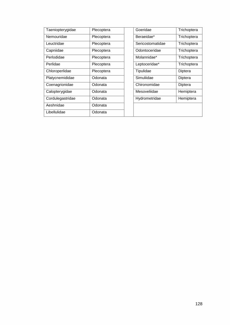
128

Taeniopterygidae Plecoptera Goeridae Trichoptera

Nemouridae Plecoptera Beraeidae* Trichoptera

Leuctridae Plecoptera Sericostomatidae Trichoptera

Capniidae Plecoptera Odontoceridae Trichoptera

Perlodidae Plecoptera Molannidae* Trichoptera

Perlidae Plecoptera Leptoceridae* Trichoptera

Chloroperlidae Plecoptera Tipulidae Diptera

Platycnemididae Odonata Simuliidae Diptera

Coenagrionidae Odonata Chironomidae Diptera

Calopterygidae Odonata Mesoveliidae Hemiptera

Cordulegastridae Odonata Hydrometridae Hemiptera

Aeshnidae Odonata

Libellulidae Odonata

129

6 General Discussion

Synthesis

6.1.1 Overview

The main aim of this thesis was to provide greater understanding of the interaction

between freshwater ecology and hydromorphology (i.e. physical habitat), with a focus

on benthic invertebrates. In particular, by employing simple, process-based

geomorphological models, it aimed to adopt a stronger conceptual underpinning than

simple species-habitat correlations. Specific knowledge gaps identified in the

literature review (Chapter 2) were the focus of subsequent chapters and included: (i)

predictions of the spatial distribution of distinct physical habitats (i.e. bedforms) using

simple models of relative riverbed mobility (Chapter 3), (ii) an assessment of the

effects of bed material and riverbed stability upon the composition and functional

diversity of invertebrate communities (Chapter 4) and (iii) an investigation of

invertebrate community response to riverbed disturbance through time (Chapter 5).

The results of these chapters have combined to provide new insights into the

interaction of physical processes and ecological communities in river systems. As

predicted, simple measures of the interaction between energy and grain size were

able to discriminate well between different physical habitat forms, despite evidence

for channel modification influencing the natural processes. Invertebrate communities

were found to be strongly connected to dominant bed material and some evidence

was found for increased flow energy (i.e. disturbance propensity) limiting the diversity

(taxonomic and functional) of communities, particularly in coarse-bedded rivers.

Evidence of riverbed disturbance acting as a temporal control on invertebrate

community composition was limited: this may have been due to the ongoing effects

of water quality.

These findings broaden current understanding of ecology-hydromorphology

interactions in river systems, particularly at large scales, and point to new tools that

could be developed to direct future river management and restoration efforts. For

example, a combination of the approaches taken in Chapter’s 3 & 4 would allow for

the design of river restoration schemes (i.e. bed material calibre, types of bedforms)

to be tailored to introduce applicable habitat for the species of interest. The approach

taken in Chapter 4 could also be developed into a tool to rapidly assess the position

of a site within the wider habitat template. This would provide river managers with a

130

way of classifying habitats with relatively low data requirements to select those where

improvement schemes would be most beneficial.

6.1.2 The distribution of physical habitats

Bars were chosen as a case study for assessing the ability of simple sediment

transport models to predict physical habitat, as they are closely linked to transport

processes, are important habitat for a range of organisms, and are recorded in detail

in River Habitat Survey i.e. different bar types and vegetation cover (Eyre et al., 2001;

Environment Agency, 2003). In this instance a very simple model of specific stream

power and mean bed material size was used to validate this possibility, which was a

key assumption for the rest of the thesis. Overall, bars were found to be readily

predictable at a national scale, with the success of predictions largely determined by

how common the bar type was. Un-vegetated bars were more readily predictable than

vegetated, likely due to their greater connectedness to the flow and sediment

transport regime, whilst alternate bars were successfully predicted most often,

followed by point and mid-channel bars. There was evidence for a threshold of

specific stream power (30 W m-2) above which bars became most common, which

was hypothesised to approximate the minimum energy required to transport gravel-

sized material. Bar prevalence was overestimated in rivers with significant

modifications or distinct flow regimes (e.g. high baseflow chalk streams). It is apparent

that the rivers where bar occurrence was overestimated due to channel modification

(Chapter 3) broadly match the rivers identified as having oversized bed material (i.e.

rivers that experience little to no bed load transport/disturbance) in Chapter 5.

Physical modification is offered as an explanation for both results, with impoundments

and flood control structures known to cause reductions in sediment supply (lack of

sediment for bar building; Petts, 1980; Brookes et al., 1983), which leads to channel

incision and bed armouring (lack of bed load transport / disturbance; Gomez, 1983).

The findings of Chapter 3 indicate that river managers need to consider that

catchment context of a river reach if interventions to restore or protect physical habitat

are to be justified and effective in the long-term.

131

6.1.3 Process-based models linking habitat with community

composition

The high taxonomic resolution (species-level) and good spatial coverage of the

RIVPACS dataset provided a unique opportunity to conduct a first-step study of the

links between sediment transport processes and invertebrate communities across

Britain (Chapter 4). The Shields regime diagram was chosen as the physical model

for this study as it provided a better link to process (e.g. bed load and suspended load

transport) than the model used in Chapter 3. The composition and function of

invertebrate communities was found to vary between rivers with gravel/cobble and

silt/sand substrates. Greater transport ability was found to reduce invertebrate

community richness, abundance and functional diversity in gravel/cobble substrates,

with traits indicative of greater resistance or resilience, such as short lifespans, aerial

dispersal and smaller aquatic stages also becoming more prevalent. In silt/sand

substrates, patterns were more complex as communities with highly-abundant taxa

became dominant with increasing transport ability, perhaps indicating that there are

fundamental differences in what constitutes disturbance (cf. gravel/cobble). The

results from gravel/cobble channels are consistent with other studies of disturbance

within rivers (e.g. Bonada et al., 2007; Larsen and Ormerod, 2010; Gutiérrez-Cánovas

et al., 2015), as well as smaller scale studies of river bed mobility (Death and

Winterbourn, 1995; Townsend et al., 1997; Miyake and Nakano, 2002), all of which

have tended to focus on gravel-bedded channels. These responses also fit with

theoretical expectations across different ecosystems (Odum, 1985), providing further

evidence of common responses to habitat variability (i.e. disturbance) across

ecosystems. Further work is needed to assess whether communities in silt/sand

channels are consistently more resistant/resilient to disturbance, or whether the

approach used here failed to capture the important characteristics of disturbance in

those rivers.

6.1.4 The temporal role of disturbance

To supplement the initial chapters which considered spatial interactions between

geomorphology and ecology, the temporal aspect of disturbance and its impact on

invertebrate communities was considered in Chapter 5. Critical specific stream power

was selected as the indicator for riverbed disturbance due to its low data requirements

and its link to the initiation of bed load transport in gravel-bed rivers (Petit, 2005;

Parker et al., 2012; 2015). This method was selected over the Shields diagram

(Chapter 4) as there is some ambiguity around the threshold of bed load transport

132

represented by the regime diagram (Mueller et al., 2005). Taxon richness, the Jaccard

index (persistence) and the prevalence of resistance and/or resilience traits were

modelled using cross sectional and longitudinal methods, with predictor variables

representing disturbance regime and water quality. The results supported the

predictions of an increase in community persistence at locations with larger or more

frequent bed disturbance, in line with previous studies (Meffe and Minckley, 1987;

Scarsbrook, 2002; Collier, 2008). However, links to richness and resistance-resilience

traits were equivocal, possibly due to water quality continuing to out-weigh the effects

of physical habitat in many streams.

Implications

The results of this thesis have several implications for the study of geomorphology –

ecology interactions in rivers. The first, based on Chapter 3 in particular, is that

physical habitat characteristics can be predicted with relative success using simple

mechanistic models, consistent with a few existing studies (e.g. Bizzi and Lerner,

2012; Vaughan et al., 2013). The focus on bars has provided a greater understanding

of the limits of and controls on their distribution, whilst also providing a proof of

concept for using models of this type to predict channel forms. This approach should

promote further integration of the traditionally separate disciplines of ecology and

geomorphology, a key requirement for the protection and restoration of river systems

into the future (Vaughan et al., 2009).

Secondly, process-based models offer a robust method of predicting community

diversity and function (Chapter 4). Understanding the factors affecting the

predictability of ecological systems, and reducing those uncertainties, is a research

priority across ecology, and capturing processes – rather than just patterns – is

thought to be an important part of this (Petchey et al. 2015). By getting closer to first

principles for both physical habitat and biology, the latter via the use of ecological

traits, process-based models should also generalise more successfully in a changing

environment (e.g. climate; Urban et al., 2016). This could provide important advances

for both pure and applied fields.

Finally, the process-based models used to link fluvial geomorphology and ecology in

this thesis are very simple (cf. fully-parameterised sediment transport equations;

Bagnold, 1966; Engelund and Fredsøe, 1976). Barriers to more widespread use of

133

mechanistic modelling in ecology and other disciplines include a limited

understanding of the underlying processes and the complexity and/or expense of

collecting data to calibrate process-based models. As a group, the sediment-transport

models used in Chapters 3–5 were simple and had minimal data requirements: their

data requirements, advantages, limitations and potential applications are summarised

in Table 6-1. All three models have wider applications for river management and

restoration planning but further development, including field verification to enhance

their links to geomorphic processes and threshold would greatly increase their power.

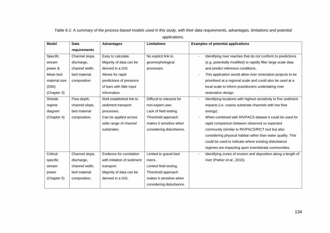
134

Table 6-1: A summary of the process-based models used in this study, with their data requirements, advantages, limitations and potential

applications.

Model Data

requirements

Advantages Limitations Examples of potential applications

Specific

stream

power &

Mean bed

material size

(D50)

(Chapter 3)

Channel slope,

discharge,

channel width,

bed material

composition.

Easy to calculate.

Majority of data can be

derived in a GIS.

Allows for rapid

predictions of presence

of bars with little input

information.

No explicit link to

geomorphological

processes.

- Identifying river reaches that do not conform to predictions

(e.g. potentially modified) to rapidly filter large scale data

and predict reference conditions.

- This application would allow river restoration projects to be

prioritised at a regional scale and could also be used at a

local scale to inform practitioners undertaking river

restoration design.

Shields

regime

diagram

(Chapter 4)

Flow depth,

channel slope,

bed material

composition.

Well established link to

sediment transport

processes.

Can be applied across

wide range of channel

substrates.

Difficult to interpret for

non-expert user.

Lack of field testing.

Threshold approach

makes it sensitive when

considering disturbance.

- Identifying locations with highest sensitivity to fine sediment

impacts (i.e. coarse substrate channels with low flow

energy).

- When combined with RIVPACS dataset it could be used for

rapid comparison between observed vs expected

community (similar to RIVPACS/RICT tool but also

considering physical habitat rather than water quality. This

could be used to indicate where existing disturbance

regimes are impacting upon invertebrate communities.

Critical

specific

stream

power

(Chapter 5)

Channel slope,

discharge,

channel width,

bed material

composition.

Evidence for correlation

with initiation of sediment

transport.

Majority of data can be

derived in a GIS.

Limited to gravel-bed

rivers.

Limited field testing.

Threshold approach

makes it sensitive when

considering disturbance.

- Identifying zones of erosion and deposition along a length of

river (Parker et al., 2015).

135

Limitations

This study has four key limitations, the first three of which are at least partly related to

the national scale at which it was conducted. This national scale is, concomitantly, one

of the strengths and novel aspects of the study, allowing questions to be asked across

spatial extents far exceeding those of conventional research funding (Vaughan and

Ormerod, 2010). The first stems from the use of secondary datasets in Chapters 3–5,

all of which had broadly the same limitations: primarily the lack of robust geomorphic

measures. For example, the measurements of mean bed sediment size used to model

bedform distribution (Chapter 3), substrate type (Chapter 4) and the threshold of

disturbance (Chapter 5) were reliant on estimates from percentage coverage or

dominant substrate type in the RIVPACS and RHS datasets, whilst the inconsistent

measurements of channel width included in the datasets were excluded in favour of

more reliable flow-width relationships (Hey and Thorne, 1986; Thayer, 2017). Other

weaknesses included using family-level resolution for the invertebrate time series data

(Chapter 5), which may mask important results (Melo, 2005), and daily mean discharge

records, rather than capturing peak discharges for characterising bed disturbance

(Chapter 5). There was also error introduced by the spatial mismatches between

sampling locations from different schemes.

The second limitation centred on the quality of the physical models. The thresholds used

to indicate the initiation of sediment transport in the critical specific stream power and

Shields regime diagram models are generally derived from laboratory flume studies

(Brownlie, 1981; Petit, 1994; Parker et al., 2012), and field testing of them is limited to a

small number of studies (e.g. Petit, 2005; Parker et al., 2007; Parker et al., 2015). These

thresholds typically do not account for variations due to bed armouring (Gomez, 1983),

fixed objects in the channel (e,g. large wood; Gurnell et al., 2002) or biotic influences

(e.g. biofilms; Stone et al., 2008; 2011 or channel vegetation; Murray and Paola, 2003).

Better, more mechanistic methods of predicting sediment transport and channel form

that account for some of this variability are available (Ackers and White, 1973; Yang,

1976; Mueller et al., 2005) but their data requirements exceed that of the available data

and their ease of calculation and interpretation is such that non-expert users (e.g. river

managers, ecologists) would be unlikely to apply them.

Thirdly, the influences on river ecosystems at a national scale are manifold, including

factors such as climate, water quality, vegetation and land use in addition to physical

habitat (Vaughan et al., 2009), whilst local-scale biotic influences (e.g. biofilms; Stone

136

et al., 2008; 2011) may also have a significant contribution. Trying to account for these

factors whilst focusing on physical habitat is a major challenge, and may contribute to

the small proportions of the variance usually explained by ecological models (Moller and

Jennions, 2002). Although additional data were available on factors such as average

water quality on a national scale, so that it was possible to control for their influence to

some extent, it is likely that they made it harder to resolve the role of sediment transport

and bed disturbance.

Finally, all of the chapters relied on correlative approaches, rather than addressing

causation directly. This is a generic problem with observational studies, but especially

with complex phenomena such as floods, where there are manifold changes to the river

environment, including water quality, habitat area or volume, and hydrological

components in addition to bed mobilisation. Although ecological relationships with bed

disturbance were found here, and attempts were made to control for factors such as

water quality, a combination of detailed, direct observations and experimental

manipulation would be needed to ascribe causal relationships with a higher degree of

confidence.

Future areas of study

The results of this study have highlighted several gaps in understanding where future

efforts should be directed. Most importantly, future studies should investigate whether

the invertebrate responses to riverbed stability noted here are replicated in other

settings. Although Britain accounts for a tiny proportion of global river length, it has a

diverse range of freshwater invertebrates and geomorphology that were captured by the

national datasets used here, yet river ecosystems in other climatic (e.g. tropical, arid)

and geologic (e.g. active mountain belts, lowland plains) settings may respond

differently (Montgomery, 1999; Boulton et al., 2008; Gallardo et al., 2014).

The consistent approach used throughout this study to link physical processes and

ecological communities based on simple, process-based models has the potential to be

developed into a series of tools for use in evidence-based river management. Greater

understanding and tools at the multi-catchment scales at which river basin management

is now planned, at least in the UK and Europe, is a key research priority (Vaughan et

al., 2009). The process-based models developed here allow for sites to be placed in

context against a baseline understanding of the likely bedforms that are typically present

(e.g. bars; Chapter 3) or invertebrate community composition (Chapter 4) using a

137

relatively small number of geomorphic variables (i.e. sediment size, channel gradient,

discharge and channel width/depth). At present, physical habitat restoration has a

relatively low level of success (Palmer et al., 2010) and significant benefits could be

derived from the use of process-based models to predict geomorphic processes,

sustainable channel forms and the resulting biological communities. A first step of any

future developments should be to validate the results of this thesis at field sites and/or

using a laboratory flume. Such studies would enable an assessment of the potential

errors inherent to these studies due to the use of secondary data and give validation to

practitioners who may wish to make use of these approaches.

Much of the novelty in this thesis has come from approaching the ecology with better

coverage of geomorphic processes. Obvious next steps would be to take a similar

approach with the ecology. Adding a phylogenetic dimension to studies of ecological

communities may provide complementary information to taxonomy and ecological traits

into the role of fluvial geomorphology, and provides a window onto evolutionary

processes. For example, measuring phylogenetic dispersion can extend the

understanding of the roles that environmental filtering and inter-specific competition play

in structuring communities relative to functional diversity measures alone (e.g. Helmus

et al., 2007; Violle et al., 2011; Cisneros et al., 2014). Stronger filters (e.g. greater river

bed disturbance) are expected to decrease phylogenetic dispersion, leading to a

community of more closely related taxa, whereas stronger inter-specific competition is

predicted to generate the opposite pattern. Work is already underway to study the

relative roles of phylogeny and habitat filtering in the formation of community trait

assemblages.

There is also potential to extend the approach used here to simple models of ecological

process, such as metabolic processes and community assembly rules (Woodward et

al., 2016). These future studies are likely to benefit from ever improving trait information

with greater coverage and resolution than that used here (e.g. Schmidt-Kloiber and

Hering, 2015), along with national datasets of greater duration, such as the routinely

sampled biological and chemical data used here, that continue to be supplemented and

made more open to public/research use (Environment Agency, 2017). There is an

opportunity for statutory environmental bodies to consolidate their sampling network

such that chemistry, biology, flow and even geomorphology are monitored at the same

locations within the river network. This would greatly increase the perceived reliability

and number of useable locations within these datasets for applications beyond routine

monitoring and allow the scale of research studies to be greatly increased with little

time/cost implications. To identify the causal mechanisms of disturbance by high flows,

138

future approaches should look to combine large scale study with experimentation that

allows other drivers (e.g. water quality) to be held constant over the period of interest.

Finally, future efforts could look to investigate how the geomorphology-ecology links

identified in this study are likely to change based on predictions of future conditions.

With the pressures faced by freshwater ecosystems expected to continue to increase

as a result of climate change, water resource use and land use change (Palmer et al.,

2008; Vorosmarty et al., 2010), this understanding is vital for undertaking effective

mitigation or restoration to protect these ecosystems and the services that they provide.

Conclusion

In short, the data presented here show evidence of an implicit link between freshwater

community composition and function, and the distribution of physical habitats. Despite

large improvements over recent decades, water quality still appears to be a key control

in terms of community structure. Both traditional and functional measures of community

diversity showed a response to changing bed material calibre and stability across large

spatial scales, consistent with other studies of habitat stability in rivers and other

ecosystems. Despite this spatial response, there was limited evidence of temporal

variability in communities as a result of riverbed disturbance, perhaps because water

quality continued to suppress the physical habitat signal. These results advance current

understanding of the role of physical habitat distribution and stability in limiting

invertebrate community composition, although more research is required to identify

whether riverbed disturbance regimes have a greater influence on invertebrate

communities as water quality stressors continue to decline. An understanding of this

relationship between physical and biological processes is of importance if management

and restoration efforts are to be successful into the future, particularly as pressures on

river ecosystems are predicted to continue to increase. The wide availability and

continued expansion of the datasets used in this study permits further development of

the approaches used here to create a series of tools, at a scale relevant for river

managers, that allow for the management decisions to be based on a scientifically

robust understanding of both hydromorphology and ecology.

139

7 References

Abelho, M. and Graça, M.A.S., 1996. Effects of eucalyptus afforestation on leaf litter dynamics and macroinvertebrate community structure of streams in Central Portugal. Hydrobiologia, 324(3), pp.195-204. Abrams, P. 1983. The theory of limiting similarity. Annual Review of Ecology and Systematics, 14, 359-376. Ackers, P. and White, W.R., 1973. Sediment transport: new approach and analysis. Journal of the Hydraulics Division, 99 (11). Alonso, A. and Castro-Diez, P., 2008. What explains the invading success of the aquatic mud snail Potamopyrgus antipodarum? Hydrobiologia, 614(1), pp.107-116. Andrews, E.D., 1979. Scour and fill in a stream channel, East Fork River, western Wyoming (No. 1117). US Govt. Print. Off. Andrews, E.D., 1980. Effective and bankfull discharges of streams in the Yampa River basin, Colorado and Wyoming. Journal of Hydrology, 46(3), pp.311-330. Andrews, E.D., 1983. Entrainment of gravel from naturally sorted riverbed material. Geological Society of America Bulletin, 94(10), pp.1225-1231. Andrews, E.D., 1994. Marginal bed load transport in a gravel bed stream, Sagehen Creek, California. Water Resources Research, 30(7), pp.2241-2250. Armitage, P.D. & Cannan, C.E. 2000. Annual changes in summer patterns of mesohabitat distribution and associated macroinvertebrate assemblages. Hydrological Processes, 14, 3161-3179. Ashmore, P.E. 1982. Laboratory modelling of gravel braided stream morphology. Earth Surface Processes and Landforms 7, pp. 201-225. Ashmore, P. E. 1991. How do gravel-bed rivers braid? Canadian Journal of Earth Sciences, 28(3), pp. 326-341. Ashworth, P.J. 1996. Mid-channel bar growth and its relationship to local flow strength and direction. Earth Surface Processes and Landforms, 21, pp. 103-123. Bachelet, D., Neilson, R.P., Lenihan, J.M. and Drapek, R.J., 2001. Climate change effects on vegetation distribution and carbon budget in the United States. Ecosystems, 4(3), pp.164-185. Bagnold, R.A., 1956. The flow of cohesionless grains in fluids. Philosophical Transactions of the Royal Society of London A: Mathematical, Physical and Engineering Sciences, 249(964), pp.235-297. Bagnold, R.A., 1966. An approach to the sediment transport problem from general physics. In: Thorne, C.R., MacArthur, R.C. and Bradley, J.B. (Eds.), The Physics of Sediment Transport by Wind and Water. American Society of Civil Engineers, New York, pp. 231-291.

Bagnold, R.A. 1977. Bed Load Transport by Natural Rivers. Water Resources Research 13(2), pp. 303-312. Bagnold, R.A. 1980. An empirical correlation of bedload transport rates in flumes and natural rivers. Proceedings of the Royal Society 372, pp. 453-473. Barbour, M.T., Graves, C.G., Plafkin, J.L., Wisseman, R.W. and Bradley, B.P., 1992. Evaluation of EPA's rapid bioassessment benthic metrics: metric redundancy and variability among reference stream sites. Environmental Toxicology and Chemistry, 11(4), pp.437-449.

140

Barker, L., Hannaford, J., Muchan, K., Turner, S and Parry, S. 2016. The winter 2015/2016 floods in the UK: a hydrological appraisal. Weather, 71, 324-333. Bathurst, J.C., Hey, R.D. and Thorne, C.R., 1979. Secondary flow and shear stress at river bends. Journal of the Hydraulics Division, 105(10), pp.1277-1295.

Beauger, A., Lair, N., Reyes-Marchant, P., & Peiry, J. (2006). The distribution of macroinvertebrate assemblages in a reach of the River Allier (France), in relation to riverbed characteristics. Hydrobiologia, 571(1), 63-76. doi: 10.1007/s10750-006-0217-x Benda, L., & Dunne, T., 1997a. Stochastic Forcing of Sediment Supply to Channel Networks from Landsliding and Debris Flow. Water Resources Research, 33(12), 2849. doi: 10.1029/97WR02388 Benda, L., & Dunne, T., 1997b. Stochastic forcing of sediment routing and storage in channel networks. Water Resources Research, 33(12), 2865. doi: 10.1029/97WR02387 Benda, L., Poff, N. L., Miller, D., Dunne, T., Reeves, G., Pess, G., & Pollock, M. 2004. The Network Dynamics Hypothesis: How Channel Networks Structure Riverine Habitats. BioScience, 54(5), pp.413-427. Berrie, A. D. 1992. The chalk-stream environment. Hydrobiologia, 248(1), 3-9. Bird, G.A. and Kaushik, N.K., 1981. Coarse particulate organic matter in streams. In Perspectives in running water ecology (pp. 41-68). Springer US. Beven, K.J., Kirkby, M.J., Schofield, N. and Tagg, A.F., 1984. Testing a physically-based flood forecasting model (TOPMODEL) for three UK catchments. Journal of Hydrology, 69(1-4), pp.119-143. Bizzi, S., and Lerner, D. N. 2012. Characterizing physical habitats in rivers using map-derived drivers of fluvial geomorphic processes. Geomorphology, 169-170, pp. 64-73. Bizzi, S., Demarchi, L., Grabowski, R.C., Weissteiner, C.J. and Van de Bund, W., 2016. The use of remote sensing to characterise hydromorphological properties of European rivers. Aquatic Sciences, 78(1), pp.57-70. Blondeaux, P. and Seminara, G., 1985. A unified bar–bend theory of river meanders. Journal of Fluid Mechanics, 157, pp.449-470. Bloomfield, J.P., Allen, D.J. and Griffiths, K.J., 2009. Examining geological controls on baseflow index (BFI) using regression analysis: An illustration from the Thames Basin, UK. Journal of Hydrology, 373(1), pp.164-176. Blöschl, G., Hall, J., Parajka, J., Perdigão, R.A., Merz, B., Arheimer, B., Aronica, G.T., Bilibashi, A., Bonacci, O., Borga, M. and Čanjevac, I., 2017. Changing climate shifts timing of European floods. Science, 357(6351), pp.588-590. Bonada, N., Doledec, S. and Statzner, B., 2007. Taxonomic and biological trait differences of stream macroinvertebrate communities between mediterranean and temperate regions: implications for future climatic scenarios. Global Change Biology, 13(8), pp.1658-1671. Bonada, N., Rieradevall, M., Prat, N. and Resh, V.H., 2006. Benthic macroinvertebrate assemblages and macrohabitat connectivity in Mediterranean-climate streams of northern California. Journal of the North American Benthological Society, 25(1), pp.32-43. Bonada, N., Rieradevall, M., & Prat, N., 2007. Macroinvertebrate community structure and biological traits related to flow permanence in a Mediterranean river network. Hydrobiologia, 589(1), 91-106. doi: 10.1007/s10750-007-0723-5 Bond, N.R. and Downes, B.J., 2000. Flow-related disturbance in streams: an experimental test of the role of rock movement in reducing macroinvertebrate population densities. Marine and Freshwater Research, 51(4), pp.333-337.

141

Boulton, A.J., Boyero, L., Covich, A.P., Dobson, M., Lake, S. and Pearson, R., 2008. Are tropical streams ecologically different from temperate streams? Tropical Stream Ecology, pp.257-284. Bradley, D and Ormerod, S.J. 2001. Community persistence among stream invertebrates tracks the North Atlantic Oscillation. J. Anim. Ecol. 70, pp.987-996 Brookes, A., Gregory, K.J. and Dawson, F.H., 1983. An assessment of river channelization in England and Wales. Science of the Total Environment, 27(2), pp.97-111. Brookes, A., 1987. River channel adjustments downstream from channelization works in England and Wales. Earth Surface Processes and Landforms, 12(4), pp.337-351. Brown, B.L., 2003. Spatial heterogeneity reduces temporal variability in stream insect communities. Ecology Letters, 6(4), pp.316-325. Brusven, M.A., and Prather, K.V., 1974. Influence of stream sediment on distribution of macrobenthos. Journal of the Entomological Society of British Columbia, 71, 24-32. Buffington, J.M. and Montgomery, D.R., 1997. A systematic analysis of eight decades of incipient motion studies, with special reference to gravel‐bedded rivers. Water Resources Research, 33(8), pp.1993-2029. Bunte, K., Abt, S.R., Swingle, K.W., Cenderelli, D.A. and Schneider, J.M., 2013. Critical Shields values in coarse‐bedded steep streams. Water Resources Research, 49(11), pp.7427-7447. Calver, A., Stewart, E. and Goodsell, G., 2009. Comparative analysis of statistical and catchment modelling approaches to river flood frequency estimation. Journal of flood risk management, 2(1), pp.24-31. Carbonneau, P., Fonstad, M.A., Marcus, W.A. and Dugdale, S.J., 2012. Making riverscapes real. Geomorphology, 137(1), pp.74-86. Carling, P., 1988. The concept of dominant discharge applied to two gravel‐bed streams in relation to channel stability thresholds. Earth Surface Processes and Landforms, 13(4), pp.355-367. Carson, M.A., Griffiths, G.A., 1987. Influence of Channel Width on Bed-Load Transport Capacity. Journal of Hydraulic Engineering-Asce, 113(12), 1489-1509. Chang, H.H. 1979. Minimum stream power and river channel patterns. Journal of Hydrology 41, pp. 303-327.

Church, M., 1995. Geomorphic response to river flow regulation: Case studies and time‐scales. River Research and Applications, 11(1), pp.3-22.

Church, M., Hassan, M.A. and Wolcott, J.F., 1998. Stabilizing self‐organized structures in gravel‐bed stream channels: Field and experimental observations. Water Resources Research, 34(11), pp.3169-3179.

Church, M., and Rice, S. P. 2009. Form and growth of bars in a wandering gravel‐bed river. Earth Surface Processes and Landforms, 34(10), pp. 1422-1432. Cisneros, L.M., Burgio, K.R., Dreiss, L.M., Klingbeil, B.T., Patterson, B.D., Presley, S.J. & Willig, M.R. 2014. Multiple dimensions of bat biodiversity along an extensive tropical elevational gradient. Journal of Animal Ecology, 83, 1124–1136. Civan, A., 2016. Phosphorus in UK Rivers: The Impact of Urban Waste Water Treatment Directive (Doctoral dissertation, Durham University). Clarke, S.E., Burnett, K.M. and Miller, D.J., 2008. Modelling Streams and Hydrogeomorphic Attributes in Oregon from Digital and Field Data1. JAWRA Journal of the American Water Resources Association, 44(2), pp.459-477.

142

Clews, E., Durance, I., Vaughan, I.P. and Ormerod, S.J. 2010. Juvenile salmonid populations in a temperate river system track synoptic trends in climate. Global Change Biology, 16, pp.3271–3283 Clifford, N.J., Harmar, O.P., Harvey, G. and Petts, G.E., 2006. Physical habitat, eco‐hydraulics and river design: a review and re‐evaluation of some popular concepts and methods. Aquatic Conservation: Marine and Freshwater Ecosystems, 16(4), pp.389-408. Cluer, B., & Thorne, C., 2014. A Stream Evolution Model Integrating Habitat and Ecosystem Benefits. River Research and Applications, 30(2), 135-154. doi: 10.1002/rra.2631 Cobb, D.G., Galloway, T.D. and Flannagan, J.F., 1992. Effects of discharge and substrate stability on density and species composition of stream insects. Canadian Journal of Fisheries and Aquatic Sciences, 49(9), pp.1788-1795. Coe, M.T., Costa, M.H. and Soares-Filho, B.S., 2009. The influence of historical and potential future deforestation on the stream flow of the Amazon River–Land surface processes and atmospheric feedbacks. Journal of Hydrology, 369(1), pp.165-174. Collier, K.J., Winterbourn, M.J. and Jackson, R.J., 1989. Impacts of wetland afforestation on the distribution of benthic invertebrates in acid streams of Westland, New Zealand. New Zealand journal of marine and freshwater research, 23(4), pp.479-490. Collier, K.J. 2008. Temporal patterns in the stability, persistence and condition of stream macroinvertebrate communities: relationships with catchment land-use and regional climate. Freshwater Biology, 53, 603-616. Collins, A., Ohandja, D.G., Hoare, D. and Voulvoulis, N., 2012. Implementing the Water Framework Directive: a transition from established monitoring networks in England and Wales. Environmental Science & Policy, 17, pp.49-61. Connell, J.H., 1978. Diversity in tropical rain forests and coral reefs. Science, 199(4335), pp.1302-1310. Corenblit, D., Baas, A.C., Bornette, G., Darrozes, J., Delmotte, S., Francis, R.A., Gurnell, A.M., Julien, F., Naiman, R.J. and Steiger, J., 2011. Feedbacks between geomorphology and biota controlling Earth surface processes and landforms: a review of foundation concepts and current understandings. Earth-Science Reviews, 106(3), pp.307-331. Corenblit, D., Tabacchi, E., Steiger, J. and Gurnell, A.M., 2007. Reciprocal interactions and adjustments between fluvial landforms and vegetation dynamics in river corridors: a review of complementary approaches. Earth-Science Reviews, 84(1), pp.56-86. Costanza, R., d'Arge, R., De Groot, R., Farber, S., Grasso, M., Hannon, B., Limburg, K., Naeem, S., O'neill, R.V., Paruelo, J. and Raskin, R.G., 1997. The value of the world's ecosystem services and natural capital. Nature, 387(6630), pp.253-260. Costanza, R., de Groot, R., Sutton, P., van der Ploeg, S., Anderson, S.J., Kubiszewski, I., Farber, S. and Turner, R.K. 2014. Changes in the global value of ecosystem services. Global Environmental Change, 26, 152–158. Coulthard, T. J., Ramirez, J., Fowler, H. J., & Glenis, V. 2012. Using the UKCP09 probabilistic scenarios to model the amplified impact of climate change on drainage basin sediment yield. Hydrology and Earth System Sciences, 16(11), 4401-4416. Crosato, A. and Mosselman, E., 2009. Simple physics-based predictor for the number of river bars and the transition between meandering and braiding. Water Resources Research, 45(3). Cummins, K.W. and Klug, M.J., 1979. Feeding ecology of stream invertebrates. Annual review of ecology and systematics, 10(1), pp.147-172.

143

Cummins, K.W., Merritt, R.W. and Andrade, P.C., 2005. The use of invertebrate functional groups to characterize ecosystem attributes in selected streams and rivers in south Brazil. Studies on Neotropical Fauna and Environment, 40(1), pp.69-89. Curran, J.C. and Wilcock, P.R., 2005. Effect of sand supply on transport rates in a gravel-bed channel. Journal of Hydraulic Engineering, 131(11), pp.961-967. Dade, W.B. and Friend, P.F., 1998. Grain-size, sediment-transport regime, and channel slope in alluvial rivers. The Journal of Geology, 106(6), pp.661-676. Dadson, S.J., Hovius, N., Chen, H., Dade, W.B., Lin, J.C., Hsu, M.L., Lin, C.W., Horng, M.J., Chen, T.C., Milliman, J. and Stark, C.P., 2004. Earthquake-triggered increase in sediment delivery from an active mountain belt. Geology, 32(8), pp.733-736. Dallas, H.F. 2007. The influence of biotope availability on macroinvertebrate assemblages in South African rivers: implications for aquatic bioassessment. Freshwater Biology, 52, 370-380. Davy-Bowker, J., Clarke, R., Furse, M., Davies, C., Corbin, T., Murphy, J. & Kneebone, N. (2007) WFD46: RIVPACS Database Documentation. Scotland and Northern Ireland Forum for Environmental Research, Edinburgh. Death, R.G. and Winterbourn, M.J., 1995. Diversity patterns in stream benthic invertebrate communities: the influence of habitat stability. Ecology, 76(5), pp.1446-1460. Death, R.G., 1995. Spatial patterns in benthic invertebrate community structure: products of habitat stability or are they habitat specific? Freshwater Biology, 33(3), pp.455-467. Death, R.G., 2002. Predicting invertebrate diversity from disturbance regimes in forest streams. Oikos, 97(1), pp.18-30. Death, R.G. and Zimmermann, E.M., 2005. Interaction between disturbance and primary productivity in determining stream invertebrate diversity. Oikos, 111(2), pp.392-402. DEFRA. 2007. Nitrates in water – the current status in England. London, Department for the Environment, Food and Rural Affairs. Demars, B.O., Kemp, J.L., Friberg, N., Usseglio-Polatera, P. and Harper, D.M., 2012. Linking biotopes to invertebrates in rivers: biological traits, taxonomic composition and diversity. Ecological Indicators, 23, pp.301-311. Diaz, A.M., Alonso, M.L.S. and Gutierrez, M.R.V.A., 2008. Biological traits of stream

macroinvertebrates from a semi‐arid catchment: patterns along complex environmental gradients. Freshwater Biology, 53(1), pp.1-21. Dietrich, W.E., 1982. Settling Velocities of Natural Particles. Water Resources Research, 18, 1615-1626. Dietrich, W.E., and Smith, J.D. 1983. Influence of the point bar on flow through curved channels. Water Resources Research 19(5), pp. 1173-1192. Ding, Y., Zang, R., Letcher, S.G., Liu, S. and He, F., 2012. Disturbance regime changes the trait distribution, phylogenetic structure and community assembly of tropical rain forests. Oikos, 121(8), pp.1263-1270. Doledec, S., Phillips, N. and Townsend, C., 2011. Invertebrate community responses to land use at a broad spatial scale: trait and taxonomic measures compared in New Zealand rivers. Freshwater Biology, 56(8), pp.1670-1688. Dollar, E.S.J., James, C.S., Rogers, K.H. and Thoms, M.C., 2007. A framework for interdisciplinary understanding of rivers as ecosystems. Geomorphology, 89(1), pp.147-162.

144

Douglas, I., 1967. Man, vegetation and the sediment yields of rivers. Nature, 215(5104), pp.925-928. Downes, B.J., Lake, P.S. and Schreiber, E.S.G., 1993. Spatial variation in the distribution of stream invertebrates: implications of patchiness for models of community organization. Freshwater Biology, 30(1), pp.119-132. Downs, P.W. and Thorne, C.R., 2000. Rehabilitation of a lowland river: reconciling flood defence with habitat diversity and geomorphological sustainability. Journal of Environmental Management, 58(4), pp.249-268. Downs, P. and Gregory, K., 2014. River channel management: towards sustainable catchment hydrosystems. Routledge. Dudgeon, D., Arthington, A.H., Gessner, M.O., Kawabata, Z.I., Knowler, D.J., Lévêque, C., Naiman, R.J., Prieur-Richard, A.H., Soto, D., Stiassny, M.L. and Sullivan, C.A., 2006. Freshwater biodiversity: importance, threats, status and conservation challenges. Biological Reviews, 81(2), pp.163-182. Durance, I., & Ormerod, S. J., 2007. Climate change effects on upland stream macroinvertebrates over a 25-year period. Global Change Biology, 13(5), 942-957. Durance, I. & Ormerod, S.J. .2009. Trends in water quality and discharge confound long term warming effects on river macroinvertebrates. Freshwater Biology, 54, 388–405. Eaton, B.C. and Lapointe, M.F., 2001. Effects of large floods on sediment transport and reach morphology in the cobble-bed Sainte Marguerite River. Geomorphology, 40(3), pp.291-309. Effenberger, M., Engel, J., Diehl, S. & Matthaei, C.D. 2008. Disturbance history influences the distribution of stream invertebrates by altering microhabitat parameters: a field experiment. Freshwater Biology, 53, 996-1011. Einstein, H.A., 1942. Formulas for the transportation of bed load. Transactions of the American Society of Civil Engineers 101, 561–597. Einstein, H. A., 1950. The bed-load function for sediment transportation in open channel flows. Washington: U.S. Dept. of Agriculture. Ekström, M., Fowler, H., Kilsby, C., & Jones, P., 2005. New estimates of future changes in extreme rainfall across the UK using regional climate model integrations. 2. Future estimates and use in impact studies. Journal of Hydrology, 300(1-4), 234-251. doi: 10.1016/j.jhydrol.2004.06.019 Emery, J.C., Gurnell, A.M., Clifford, N.J. and Petts, G.E., 2004. Characteristics and controls of gravel-bed riffles: An analyses of data from the River Habitat Survey. Water and Environment Journal, 18(4), pp.210-216. Engelund, F. and Hansen, E., 1967. A monograph on sediment transport in alluvial streams. Technical University of Denmark 0stervoldgade 10, Copenhagen K. Environment Agency. 2002. Rivers and Estuaries – A Decade of Improvement. Environment Agency, Bristol. Engelund, F. and Fredsøe, J., 1976. A sediment transport model for straight alluvial channels. Hydrology Research, 7(5), pp.293-306. Environment Agency., 2003. River Habitat Survey in Britain and Ireland: Field Survey Guidance Manual, Environment Agency, Bristol, UK. Environment Agency. 2017. Water Quality Archive. Accessed on 12th September 2017 at http://environment.data.gov.uk/water-quality/view/landing.

145

European Commission. 2000. Directive 2000/60/EEC, Establishing a framework for community action in the field of water policy. Official Journal of the European Communities L327: 1–71, Brussels. Evans, R., Collins, A.L., Foster, I.D.L., Rickson, R.J., Anthony, S.G., Brewer, T., Deeks, L., Newell-Price, J.P., Truckell, I.G. & Zhang, Y. 2016. Extent, frequency and rate of water erosion of arable land in Britain - benefits and challenges for modelling. Soil Use and Management, 32, 149-161. Everard, M., 2004. Investing in sustainable catchments. Science of the Total Environment, 324(1), pp.1-24. Extence, C.A., 1981. The effect of drought on benthic invertebrate communities in a lowland river. Hydrobiologia, 83(2), pp.217-224. Eyre, M. D., Luff, M. L., & Phillips, D. A. 2001. The ground beetles (Coleoptera: Carabidae) of exposed riverine sediments in Scotland and northern England. Biodiversity & Conservation, 10(3), 403-426. Ferguson, R.I. 1981. Channel form and channel changes. In: British Rivers (Ed. Lewin, J.). London: George Allen and Unwin, pp. 90-125. Ferguson, R.I. 1987. Hydraulic and sedimentary controls of channel pattern. In River Channels: environment and process (Ed. Richards, K.S.). Oxford: Blackwell, pp. 129-58. Ferguson, R.I., 2005. Estimating critical stream power for bedload transport calculations in gravel-bed rivers. Geomorphology, 70(1), pp.33-41. Ferreira, V. and Chauvet, E., 2011. Synergistic effects of water temperature and dissolved nutrients on litter decomposition and associated fungi. Global Change Biology, 17(1), pp.551-564. Fill, H.D. and Steiner, A.A., 2003. Estimating instantaneous peak flow from mean daily flow data. Journal of Hydrologic Engineering, 8(6), pp.365-369. Fisher, G.B., Bookhagen, B. and Amos, C.B., 2013. Channel planform geometry and slopes from freely available high-spatial resolution imagery and DEM fusion: Implications for channel width scalings, erosion proxies, and fluvial signatures in tectonically active landscapes. Geomorphology, 194, pp.46-56. Fisher, S.G., Heffernan, J.B., Sponseller, R.A. and Welter, J.R., 2007. Functional ecomorphology: feedbacks between form and function in fluvial landscape ecosystems. Geomorphology, 89(1), pp.84-96. Flecker, A.S. and Feifarek, B., 1994. Disturbance and the temporal variability of invertebrate assemblages in two Andean streams. Freshwater Biology, 31(2), pp.131-142. Fox, J.W., 2013. The intermediate disturbance hypothesis should be abandoned. Trends in ecology & evolution, 28(2), pp.86-92. Friedman, J.M., Osterkamp, W.R., Lewis, W.M., 1996. The role of vegetation and bed-level fluctuations in the process of channel narrowing. Geomorphology, 14(4), 341-351. Frissell, C.A., Liss, W.J., Warren, C.E. and Hurley, M.D., 1986. A hierarchical framework for stream habitat classification: viewing streams in a watershed context. Environmental Management, 10(2), pp.199-214. Gallardo, B., Dolédec, S., Paillex, A., Arscott, D.B., Sheldon, F., Zilli, F., Mérigoux, S., Castella, E. and Comín, F.A., 2014. Response of benthic macroinvertebrates to gradients in hydrological connectivity: a comparison of temperate, subtropical, Mediterranean and semiarid river floodplains. Freshwater Biology, 59(3), pp.630-648.

146

Garner, G., Hannah, D. M., Sadler, J. P., & Orr, H. G., 2013. River temperature regimes of England and Wales: Spatial patterns, inter-annual variability and climatic sensitivity. Hydrological Processes. doi: 10.1002/hyp.9992 Gibbins, C., Vericat, D. and Batalla, R.J., 2007. When is stream invertebrate drift catastrophic? The role of hydraulics and sediment transport in initiating drift during flood events. Freshwater Biology, 52(12), pp.2369-2384. Gomez, B., 1983. Temporal variations in bedload transport rates: the effect of progressive bed armouring. Earth Surface Processes and Landforms, 8(1), pp.41-54. Gomez, B. and Church, M., 1989. An assessment of bed load sediment transport formulae for gravel bed rivers. Water Resources Research, 25(6), pp.1161-1186. Goudie, A.S., 2006. Global warming and fluvial geomorphology. Geomorphology, 79(3), pp.384-394. Graham, N.A., Jennings, S., MacNeil, M.A., Mouillot, D. and Wilson, S.K., 2015. Predicting climate-driven regime shifts versus rebound potential in coral reefs. Nature, 518(7537), pp.94-97. Griffiths, M., 2002. The European Water Framework Directive: an approach to integrated river basin management. European Water Management Online, 5, pp.1-14. Gulis, V., Ferreira, V. and Graça, M.A.S., 2006. Stimulation of leaf litter decomposition and associated fungi and invertebrates by moderate eutrophication: implications for stream assessment. Freshwater Biology, 51(9), pp.1655-1669. Gurnell, A.M., Piegay, H., Swanson, F.J. and Gregory, S.V., 2002. Large wood and fluvial processes. Freshwater Biology, 47(4), pp.601-619. Gurnell, A.M., O'Hare, J.M., O'Hare, M.T., Dunbar, M.J. and Scarlett, P.M., 2010. An exploration of associations between assemblages of aquatic plant morphotypes and channel geomorphological properties within British rivers. Geomorphology, 116(1), pp.135-144. Gurtz, M. E., & Wallace, J. B., 1984. Substrate-Mediated Response of Stream Invertebrates to Disturbance. Ecology, 65(5), 1556. doi: 10.2307/1939135 Gutiérrez-Cánovas, C., Sánchez-Fernández, D., Velasco, J., Millán, A. and Bonada, N., 2015. Similarity in the difference: changes in community functional features along natural and anthropogenic stress gradients. Ecology, 96(9), pp.2458-2466. Hannaford, J. and Marsh, T., 2006. An assessment of trends in UK runoff and low flows using a network of undisturbed catchments. International Journal of Climatology, 26(9), pp.1237-1253. Harrell, F. E. 2001. Regression modelling strategies. Springer Science & Business Media, New York. Harvey, G.L., Gurnell, A.M. and Clifford, N.J., 2008. Characterisation of river reaches: The influence of rock type. Catena, 76(1), pp.78-88. Harvey, G. L., Clifford, N. J., & Gurnell, A. M., 2008. Towards an ecologically meaningful classification of the flow biotope for river inventory, rehabilitation, design and appraisal purposes. Journal of Environmental Management, 88(4), 638-650. doi: 10.1016/j.jenvman.2007.03.039 Hastie, L., Cooksley, S., Scougall, F., Young, M., Boon, P., & Gaywood, M., 2003. Characterization of freshwater pearl mussel (Margaritifera margaritifera) riverine habitat using River Habitat Survey data. Aquatic Conservation: Marine and Freshwater Ecosystems, 13(3), 213-224. doi: 10.1002/aqc.560

147

Hawkins, C. P., Murphy, M. L., & Anderson, N. H., 1982. Effects of Canopy, Substrate Composition, and Gradient on the Structure of Macroinvertebrate Communities in Cascade Range Streams of Oregon. Ecology, 63(6), 1840. doi: 10.2307/1940125 Helmus, M.R., Savage, K., Diebel, M.W., Maxted, J.T. & Ives, A.R. 2007. Separating the determinants of phylogenetic community structure. Ecology Letters, 10, 917–925. Henriques, C., Garnett, K., Weatherhead, E.K., Lickorish, F.A., Forrow, D. and Delgado, J., 2015. The future water environment—Using scenarios to explore the significant water management challenges in England and Wales to 2050. Science of the Total Environment, 512, pp.381-396. Hey, R. D., and Thorne, C. R. 1986. Stable channels with mobile gravel beds. Journal of Hydraulic Engineering, 112(8), pp. 671-689. Hickin, E.J., 1984. Vegetation and river channel dynamics. The Canadian Geographer, 28(2), pp.111-126. Hobbs, R.J. and Huenneke, L.F., 1992. Disturbance, diversity, and invasion: implications for conservation. Conservation Biology, 6(3), pp.324-337. Hoey, T.B. and Ferguson, R., 1994. Numerical simulation of downstream fining by selective transport in gravel bed rivers: Model development and illustration. Water Resources Research, 30(7), pp.2251-2260. Hooke, J.M. 1986. The significance of mid-channel bars in an active meandering river. Sedimentology 33(6), pp. 839-850. Hooke, J., 2003. Coarse sediment connectivity in river channel systems: a conceptual framework and methodology. Geomorphology, 56(1), pp.79-94. Hooke, J.M. and Yorke, L., 2011. Channel bar dynamics on multi-decadal timescales in an active meandering river. Earth Surface Processes and Landforms, 36(14), pp.1910-1928. Hughes, J.M., 2007. Constraints on recovery: using molecular methods to study connectivity of aquatic biota in rivers and streams. Freshwater Biology, 52(4), pp.616-631. Hynes, H.B.N., 1958. The effect of drought on the fauna of a small mountain stream in Wales. Verhandlungen der Internationalen Vereinigung für theoretische und angewandte Limnologie, 8, pp.826-833. Jaccard, P., 1908. Nouvelles researches sur la distribution florale. Bull Soc Vaud Sci Nat, 44, pp.223-270. Jain, V., Preston, N., Fryirs, K. and Brierley, G., 2006. Comparative assessment of three approaches for deriving stream power plots along long profiles in the upper Hunter River catchment, New South Wales, Australia. Geomorphology, 74(1-4), pp.297-317. Jeffers, J., 1998. Characterization of river habitats and prediction of habitat features using ordination techniques. Aquatic Conservation: Marine and Freshwater Ecosystems, 8(4), 529-540. doi: 10.1002/(SICI)1099-0755(199807/08)8:43.0.CO;2-9 Jeffers, J.N.R., 1998. The statistical basis of sampling strategies for rivers: an example using River Habitat Survey. Aquatic Conservation: Marine and Freshwater Ecosystems, 8(4), pp.447-454. Johnson, A.C., Acreman, M.C., Dunbar, M.J., Feist, S.W., Giacomello, A.M., Gozlan, R.E., Hinsley, S.A., Ibbotson, A.T., Jarvie, H.P., Jones, J.I. and Longshaw, M., 2009. The British river of the future: how climate change and human activity might affect two contrasting river ecosystems in England. Science of the Total Environment, 407(17), pp.4787-4798.

148

Johnson, W.W. and Finley, M.T., 1980. Handbook of acute toxicity of chemicals to fish and aquatic invertebrates: Summaries of toxicity tests conducted at Columbia National Fisheries Research Laboratory, 1965-78(No. 137). US Fish and Wildlife Service. Jones, J.I., Duerdoth, C.P., Collins, A.L., Naden, P.S. & Sear, D.A. 2014. Interactions between diatoms and fine sediment. Hydrological Processes, 28, 1226-1237

Jowett, I.G., 2003. Hydraulic constraints on habitat suitability for benthic invertebrates in gravel‐bed rivers. River Research and Applications, 19(5‐6), pp.495-507. Kelly, D.W., Dick, J.T.A., Montgomery, W.I. and MacNeil, C., 2003. Differences in composition of macroinvertebrate communities with invasive and native Gammarus spp.(Crustacea: Amphipoda). Freshwater Biology, 48(2), pp.306-315. Kemp, J. L., Harper, D. M., & Crosa, G. A., 2000. The habitat-scale ecohydraulics of rivers. Ecological Engineering, 16(1), 17-29. doi: 10.1016/S0925-8574(00)00073-2 Kemp, P., Sear, D., Collins, A., Naden, P. & Jones, I. 2011 The impacts of fine sediment on riverine fish. Hydrological Processes, 25, 1800-1821 Kendon, E.J., Roberts, N.M., Fowler, H.J., Roberts, M.J., Chan, S.C. & Senior, C.A. 2014.

Heavier summer downpours with climate change revealed by weather forecast resolution model.

Nature Climate Change, 4, 570–576.

Kjeldsen, T. R., Jones, D. A., and Bayliss, A. C. 2008. Improving the FEH statistical procedures for flood frequency estimation. Bristol: Environment Agency. Kleinhans, M. G. 2010. Sorting out river channel patterns. Progress in Physical Geography, 34(3), pp. 287-326. Kleinhans, M.G. and van den Berg, J.H. 2011. River channel and bar patterns explained and predicted by an empirical and physics-based method. Earth Surface Processes and Landforms 36, pp. 721-738. Knighton, A.D., 1972. Changes in a braided reach. Geological Society of America Bulletin 83, 3813–3822. Knighton, D., 1998. Fluvial forms and processes: a new perspective. Routledge, Oxon, UK. Kusnierz, P.C., Holbrook, C.M. and Feldman, D.L., 2015. An evaluation of a bed instability index as an indicator of habitat quality in mountain streams of the northwestern United States. Environmental Monitoring and Assessment, 187(8), p.511. Lake, P.S., 2000. Disturbance, patchiness, and diversity in streams. Journal of the North American Benthological Society, 19(4), pp.573-592. Lammert, M., & Allan, J. D., 1999. Environmental Auditing: Assessing Biotic Integrity of Streams: Effects of Scale in Measuring the Influence of Land Use/Cover and Habitat Structure on Fish and Macroinvertebrates. Environmental Management, 23(2), 257-270. doi: 10.1007/s002679900184 Lamouroux, N., Dolédec, S. and Gayraud, S., 2004. Biological traits of stream macroinvertebrate communities: effects of microhabitat, reach, and basin filters. Journal of the North American Benthological Society, 23(3), pp.449-466. Langford, T.E.L., Shaw, P.J., Ferguson, A.J.D., Howard, S.R. 2009. Long-term recovery of macroinvertebrate biota in grossly polluted streams: re-colonisation as a constraint to ecological quality. Ecological Indicators, 9, 1064–1077. Langton, S. D., Briggs, P. A., & Haysom, K. A., 2010. Daubenton's bat distribution along rivers - developing and testing a predictive model. Aquatic Conservation: Marine and Freshwater Ecosystems, 20(S1), S45-S54. doi: 10.1002/aqc.1077

149

Larimore, R.W., Childers, W.F. and Heckrotte, C., 1959. Destruction and re-establishment of stream fish and invertebrates affected by drought. Transactions of the American Fisheries Society, 88(4), pp.261-285. Larsen, S., Vaughan, I. P., & Ormerod, S. J., 2009. Scale-dependent effects of fine sediments on temperate headwater invertebrates. Freshwater Biology, 54(1), 203-219. Larsen, S. and Ormerod, S.J., 2010. Combined effects of habitat modification on trait composition and species nestedness in river invertebrates. Biological Conservation, 143(11), pp.2638-2646. Larsen, S., & Ormerod, S. J., 2010. Low-level effects of inert sediments on temperate stream invertebrates. Freshwater Biology, 55(2), 476-486. doi: 10.1111/j.1365-2427.2009.02282.x Lawler, D.M., Petts, G.E., Foster, I.D. and Harper, S., 2006. Turbidity dynamics during spring storm events in an urban headwater river system: The Upper Tame, West Midlands, UK. Science of the Total Environment, 360(1), pp.109-126. Lee L, Helsel D (2005) Statistical analysis of water-quality data containing multiple detection limits: S-language software for regression on order statistics. Computers and Geosciences, 31, 1241–1248. Legendre, P. and Legendre, L. 1998. Numerical ecology: second English edition. Developments in Environmental Modelling, 20. Legleiter, C.J., Roberts, D.A., Marcus, A. and Fonstad, M.A. 2004. Passive optical remote sensing of river channel morphology and in-stream habitat: Physical basis and feasibility. Remote Sensing of the Environment 93(4), pp. 493-510. Lenat, D.R., 1988. Water quality assessment of streams using a qualitative collection method for benthic macroinvertebrates. Journal of the North American Benthological Society, 7(3), pp.222-233. Leopold, L. B., and Wolman, M. G. 1957. River Channel Patterns: Braided, Meandering, and Straight. Geographical Survey Professional Paper 282. Lewin, J. 1976. Initiation of bed forms and meander in coarse-grained sediment. Geological Society of America Bulletin 87(2), pp. 281-285. Lewin, J. (1981) British Rivers. Harper Collins. Lisle, T.E., Ikeda, H. and Iseya, F. 1991. Formation of Stationary Alternate Bars in a Steep Channel with Mixed-size Sediment: A Flume Experiment. Earth Surface Processes and Landforms 16, pp. 463-469. Lisle, T.E., Iseya, F. and Ikeda, H., 1993. Response of a channel with alternate bars to a decrease in supply of mixed‐size bed load: A flume experiment. Water Resources Research, 29(11), pp.3623-3629. Lisle, T.E., Nelson, J.M., Pitlick, J., Madej, M.A. and Barkett, B.L. 2000. Variability of bed mobility in natural, gravel-bed channels and adjustements to sediment load at local and reach scales. Water Resources Research 36(12), pp. 3743-3755. Lobera, G., Muñoz, I., López-Tarazón, J.A., Vericat, D. and Batalla, R.J., 2017. Effects of flow regulation on river bed dynamics and invertebrate communities in a Mediterranean river. Hydrobiologia, 784(1), pp.283-304. Luchi, R., Hooke, J.M., Zolezzi, G. and Bertoldi, W., 2010a. Width variations and mid-channel bar inception in meanders: River Bollin (UK). Geomorphology, 119(1), pp.1-8.

Luchi, R., Zolezzi, G. and Tubino, M., 2010b. Modelling mid‐channel bars in meandering channels. Earth Surface Processes and Landforms, 35(8), pp.902-917.

150

Lytle, D.A., 2003. Reconstructing long-term flood regimes with rainfall data: effects of flood timing on caddisfly populations. The Southwestern Naturalist, 48(1), pp.36-42. Mackey, R.L. and Currie, D.J., 2001. The diversity–disturbance relationship: is it generally strong and peaked?. Ecology, 82(12), pp.3479-3492. Mackin, J. H. 1948. Concept of the graded river. Geological Society of America Bulletin, 59(5), pp. 463-512. Macklin, M. G., & Lewin, J. 2003. Rapid Communication River sediments, great floods and centennial-scale Holocene climate change. Journal of Quaternary Science, 18(2), 101-105. Madej, M.A., Ozaki, V., 1996. Channel response to sediment wave propagation and movement, Redwood Creek, California, USA. Earth Surface Processes and Landforms, 21(10), 911-927. Madsen, J. D., Chambers, P. A., James, W. F., Koch, E. W., & Westlake, D. F. 2001. The interaction between water movement, sediment dynamics and submersed macrophytes. Hydrobiologia, 444(1-3), 71-84. Magurran, A.E. 2004. Measuring Biological Diversity. Blackwell Science, Malden, MA. Mallakpour, I. and Villarini, G., 2015. The changing nature of flooding across the central United States. Nature Climate Change, 5(3), p.250. Maltby, E., Ormerod, S., Acreman, M., Dunbar, M., Jenkins, A., Maberly, S., Newman, J., Blackwell, M. and Ward, R., 2011. Chapter 9 - Freshwaters: openwaters, wetlands and floodplains. In: The UK National Ecosystem Assessment Technical Report. UK National Ecosystem Assessment, UNEP-WCMC, Cambridge.

Manchester, S.J. and Bullock, J.M., 2000. The impacts of non‐native species on UK biodiversity and the effectiveness of control. Journal of Applied Ecology, 37(5), pp.845-864. Mao, L., Cooper, J.R. and Frostick, L.E., 2011. Grain size and topographical differences between static and mobile armour layers. Earth Surface Processes and Landforms, 36(10), pp.1321-1334. Markovic, D., Carrizo, S., Freyhof, J., Cid, N., Lengyel, S., Scholz, M., Kasperdius, H. and Darwall, W., 2014. Europe's freshwater biodiversity under climate change: distribution shifts and conservation needs. Diversity and Distributions, 20(9), pp.1097-1107. Mason, C.F., 2002. Biology of freshwater pollution. Pearson Education. Mason, N.W., Mouillot, D., Lee, W.G. and Wilson, J.B., 2005. Functional richness, functional evenness and functional divergence: the primary components of functional diversity. Oikos, 111(1), pp.112-118. May, C. L., & Lisle, T. E., 2012. River profile controls on channel morphology, debris flow disturbance, and the spatial extent of salmonids in steep mountain streams. Journal of Geophysical Research, 117. doi: 10.1029/2011JF002324 McCabe, D. J., & Gotelli, N. J., 2000. Effects of disturbance frequency, intensity, and area on assemblages of stream macroinvertebrates. Oecologia, 124(2), 270-279. doi: 10.1007/s004420000369 McCluney, K.E., Poff, N.L., Palmer, M.A., Thorp, J.H., Poole, G.C., Williams, B.S., Williams, M.R. and Baron, J.S. 2014. Riverine macrosystems ecology: sensitivity, resistance, and resilience of whole river basins with human alterations. Frontiers in Ecology and the Environment, 12(1), 48-58.

151

McGill, B.J., Enquist, B.J, Weiher, E. & Westoby, M. (2006.) Rebuilding community ecology from functional traits. Trends in Ecology and Evolution, 21, 178–185 Meffe, G.K. and Minckley, W.L., 1987. Persistence and stability of fish and invertebrate assemblages in a repeatedly disturbed Sonoran Desert stream. American Midland Naturalist, pp.177-191. Melo, A.S., 2005. Effects of taxonomic and numeric resolution on the ability to detect ecological patterns at a local scale using stream macroinvertebrates. Archiv für Hydrobiologie, 164(3), pp.309-323. Menge, B.A. and Sutherland, J.P., 1987. Community regulation: variation in disturbance, competition, and predation in relation to environmental stress and recruitment. The American Naturalist, 130(5), pp.730-757. Metcalfe, J.L., 1989. Biological water quality assessment of running waters based on macroinvertebrate communities: history and present status in Europe. Environmental pollution, 60(1-2), pp.101-139. Meyer-Peter, E. and Müller, R., 1948. Formulas for bed-load transport. In IAHSR 2nd meeting, Stockholm, appendix 2. IAHR. Miller, A.D., Roxburgh, S.H. and Shea, K. 2010 How frequency and intensity shape diversity–disturbance relationships. PNAS, 108, 5643–5648. Milner, A.M., Conn, S.C. & Brown, L.E. 2006. Persistence and stability of macroinvertebrate communities in streams of Denali National Park, Alaska: implications for biological monitoring. Freshwater Biology, 51, 373–387. Miyake, Y. and Nakano, S., 2002. Effects of substratum stability on diversity of stream invertebrates during baseflow at two spatial scales. Freshwater Biology, 47(2), pp.219-230. Møller, A. and Jennions, M.D., 2002. How much variance can be explained by ecologists and evolutionary biologists? Oecologia, 132(4), pp.492-500. Monaghan KA, Soares AMVM., 2012. Bringing new knowledge to an old problem: building a biotic index from lotic macroinvertebrate traits. Ecological Indicators, 20, 213–220. Montgomery, D.R. and Buffington, J.M., 1997. Channel-reach morphology in mountain drainage basins. Geological Society of America Bulletin, 109(5), pp.596-611. Montgomery, D.R., Dietrich, W.E. and Sullivan, K. 1998. The role of GIS in watershed analysis. In: Landform Monitoring, Modelling and Analysis, SN Land, KS Richards, and JH Chandler (Editors). John Wiley and Sons, Hoboken, New Jersey, pp.241-261. Montgomery, D.R., 1999. Process domains and the river continuum. JAWRA Journal of the American Water Resources Association, 35(2), pp.397-410. Morris D G, 2003. Automation and appraisal of the FEH statistical procedures for flood frequency estimation. Report to Defra, Centre for Ecology & Hydrology. Mouchet, M.A., Villéger, S., Mason, N.W. and Mouillot, D., 2010. Functional diversity measures: an overview of their redundancy and their ability to discriminate community assembly rules. Functional Ecology, 24(4), pp.867-876. Mouillot, D., Graham, N.A., Villéger, S., Mason, N.W. and Bellwood, D.R., 2013. A functional approach reveals community responses to disturbances. Trends in Ecology & Evolution, 28(3), pp.167-177. Mueller, E.R., Pitlick, J. and Nelson, J.M., 2005. Variation in the reference Shields stress for bed load transport in gravel‐bed streams and rivers. Water Resources Research, 41(4).

152

Murphy, J.M., Sexton, D.M., Jenkins, G.J., Booth, B.B., Brown, C.C., Clark, R.T., Collins, M., Harris, G.R., Kendon, E.J., Betts, R.A. and Brown, S.J., 2009. UK climate projections science report: climate change projections. Murray-Bligh JAD, Furse MT, Jones FH, Gunn RJM, Dines RA and Wright JF. 1997. Procedure for collecting and analysing macroinvertebrate samples for RIVPACS. Environment Agency, Bristol. Murray, A.B. and Paola, C., 2003. Modelling the effect of vegetation on channel pattern in bedload rivers. Earth Surface Processes and Landforms, 28(2), pp.131-143. Naeem, S., Duffy, J.E. and Zavaleta, E., 2012. The functions of biological diversity in an age of extinction. Science, 336(6087), pp.1401-1406. Naegeli, M.W., Hartmann, U., Meyer, E.I. and Uehlinger, U., 1995. POM-dynamics and community respiration in the sediments of a floodprone prealpine river (Necker, Switzerland). Archiv für Hydrobiologie, 133(3), pp.339-347. Nanson, G. C. 1980. Point bar and floodplain formation of the meandering Beatton River, Northeastern British Columbia, Canada. Sedimentology, 27(1), pp. 3-29. Nanson, G. C., and Croke, J. C. 1992. A genetic classification of floodplains. Geomorphology, 4(6), pp. 459-486. Nash, J.E. and Sutcliffe, J.V., 1970. River flow forecasting through conceptual models part I—A discussion of principles. Journal of Hydrology, 10(3), pp.282-290. Naura, M., & Robinson, M., 1998. Principles of using River Habitat Survey to predict the distribution of aquatic species: An example applied to the native white-clawed crayfish Austropotamobius pallipes. Aquatic Conservation: Marine and Freshwater Ecosystems, 8(4), 515-527. doi: 10.1002/(SICI)1099-0755(199807/08)8:43.0.CO;2-J Neeson, T.M., Gorman, A.M., Whiting, P.J. and Koonce, J.F., 2008. Factors affecting accuracy of stream channel slope estimates derived from geographical information systems. North American Journal of Fisheries Management, 28(3), pp.722-732. Newson, M. D., Clark, M. J., Sear, D. A., and Brookes, A. 1998a. The geomorphological basis for classifying rivers. Aquatic Conservation: Marine and Freshwater Ecosystems, 8(4), pp. 415-430. Newson, M.D., Harper, D.M., Padmore, C.L., Kemp, J.L. & Vogel, B. 1998b. A cost-effective approach for linking habitats, flow types and species requirements. Aquatic Conservation: Marine and Freshwater Ecosystems, 8, 431–446. Newson, M.D. and Newson, C.L., 2000. Geomorphology, ecology and river channel habitat: mesoscale approaches to basin-scale challenges. Progress in Physical Geography, 24(2), pp.195-217. Newson, M.D., 2002. Geomorphological concepts and tools for sustainable river ecosystem management. Aquatic Conservation: Marine and Freshwater Ecosystems, 12(4), pp.365-379. Newson, M. D., & Large, A. R., 2006. ‘Natural’ rivers, ‘hydromorphological quality’ and river restoration: A challenging new agenda for applied fluvial geomorphology. Earth Surface Processes and Landforms, 31(13), 1606-1624. doi: 10.1002/esp.1430 Odum, E.P. 1985 Trends expected in stressed ecosystems. BioScience, 35, pp.419-422. Parker, G., 1990. Surface-based bedload transport relation for gravel rivers. Journal of Hydraulic Research, 28(4), pp.417-436. Jari Oksanen, F. Guillaume Blanchet, Michael Friendly, Roeland Kindt, Pierre Legendre, Dan McGlinn, Peter R. Minchin, R. B. O'Hara, Gavin L. Simpson, Peter Solymos, M. Henry H.

153

Stevens, Eduard Szoecs and Helene Wagner (2017). vegan: Community Ecology Package. R package version 2.4-3. https://CRAN.R-project.org/package=vegan Olden, J.D. and Poff, N.L., 2003. Redundancy and the choice of hydrologic indices for characterizing streamflow regimes. River Research and Applications, 19(2), pp.101-121. Olsen, D.A. and Townsend, C.R., 2005. Flood effects on invertebrates, sediments and particulate organic matter in the hyporheic zone of a gravel‐bed stream. Freshwater Biology, 50(5), pp.839-853. Olsson, T.I., 1981. Overwintering of benthic macroinvertebrates in ice and frozen sediment in a North Swedish river. Ecography, 4(3), pp.161-166. Ormerod, S.J. and Durance, I., 2009. Restoration and recovery from acidification in upland Welsh streams over 25 years. Journal of Applied Ecology, 46(1), pp.164-174. Orr, H. G., Large, A. R. G., Newson, M. D., and Walsh, C. L. 2008. A predictive typology for characterising hydromorphology. Geomorphology, 100(1), pp. 32-40. Oudin, L., Hervieu, F., Michel, C., Perrin, C., Andréassian, V., Anctil, F., & Loumagne, C., 2005. Which potential evapotranspiration input for a lumped rainfall–runoff model? Journal of Hydrology, 303(1-4), 290-306. doi: 10.1016/j.jhydrol.2004.08.026 Padmore, C., 1998. The role of physical biotopes in determining the conservation status and flow requirements of British rivers. Aquatic Ecosystem Health & Management, 1(1), 25-35. doi: 10.1080/14634989808657003 Palmer, M.A., Reidy Liermann, C.A., Nilsson, C., Flörke, M., Alcamo, J., Lake, P.S. and Bond, N., 2008. Climate change and the world's river basins: anticipating management options. Frontiers in Ecology and the Environment, 6(2), pp.81-89. Palmer, M.A., Menninger, H.L. & Bernhardt, E. 2010. River restoration, habitat heterogeneity and biodiversity: a failure of theory or practice? Freshwater biology, 55, 205–222. Parker, R.N., Hales, T.C., Mudd, S.M., Grieve, S.W. and Constantine, J.A., 2016. Colluvium supply in humid regions limits the frequency of storm-triggered landslides. Scientific reports, 6, p.34438. Parker, C., Clifford, N. J., and Thorne, C. R. 2011. Understanding the influence of slope on the threshold of coarse grain motion: Revisiting critical stream power. Geomorphology, 126(1), pp. 51-65. Parker, C., Clifford, N. J., & Thorne, C. R., 2012. Automatic Delineation Of Functional River Reach Boundaries For River Research And Applications. River Research and Applications, 28(10), 1708-1725. doi: 10.1002/rra.1568

Parker, C., Thorne, C.R. and Clifford, N.J., 2015. Development of ST: REAM: a reach‐based stream power balance approach for predicting alluvial river channel adjustment. Earth Surface Processes and Landforms, 40(3), pp.403-413. Parker, G. 1976. On the cause and characteristic scales of meandering and braiding in rivers. Journal of Fluid Mechanics 76(3), pp. 457-480. Parker, G., Seminara, G. and Solari, L., 2003. Bed load at low Shields stress on arbitrarily sloping beds: Alternative entrainment formulation. Water Resources Research, 39(7).

Parker, G., Wilcock, P.R., Paola, C., Dietrich, W.E. and Pitlick, J., 2007. Physical basis for quasi‐universal relations describing bankfull hydraulic geometry of single‐thread gravel bed rivers. Journal of Geophysical Research: Earth Surface, 112(F4).

154

Parr, L., & Mason, C., 2003. Long-term trends in water quality and their impact on macroinvertebrate assemblages in eutrophic lowland rivers. Water Research, 37(12), 2969-2979. doi: 10.1016/S0043-1354(03)00115-5 Pedersen, M. L., Friberg, N., & Larsen, S. E., 2004. Physical habitat structure in Danish lowland streams. River Research and Applications, 20(6), 653-669. doi: 10.1002/rra.770 Pedersen, M. L., & Friberg, N., 2007. Two lowland stream riffles – linkages between physical habitats and macroinvertebrates across multiple spatial scales. Aquatic Ecology, 41(3), 475-490. doi: 10.1007/s10452-004-1584-x Percival, E., & Whitehead, H., 1929. A Quantitative Study of the Fauna of Some Types of Stream-Bed. The Journal of Ecology, 17(2), 282. doi: 10.2307/2256044 Petchey, O.L., Pontarp, M., Massie,T.M., Kefi, S., Ozgul, A., Weilenmann, M., Palamara, G.M., Altermatt, F., Matthews, B., Levine, J.M., Childs, D.Z., McGill, B.J., Schaepman, M.E., Schmid, B., Spaak, P., Beckerman, A.P., Pennekamp, F. & Pearse, I.S. 2015. The ecological forecast horizon, and examples of its uses and determinants. Ecology Letters, 18, 597–611. Petit, F., 1994. Dimensionless critical shear stress evaluation from flume experiments using different gravel beds. Earth Surface Processes and Landforms, 19(6), pp.565-576. Petit, F., Poinsart, D. and Bravard, J.P., 1996. Channel incision, gravel mining and bedload transport in the Rhône river upstream of Lyon, France (“canal de Miribel”). Catena, 26(3-4), pp.209-226. Petit, F., Gob, F., Houbrechts, G., & Assani, A. A. 2005. Critical specific stream power in gravel-bed rivers. Geomorphology, 69(1), pp. 92-101. Petts, G.E., 1980. Long-term consequences of upstream impoundment. Environmental Conservation, 7(4), pp.325-332. Petts, G.E., 2009. Instream flow science for sustainable river management. JAWRA Journal of the American Water Resources Association, 45(5), pp.1071-1086. Phillips, C.B. and Jerolmack, D.J., 2016. Self-organization of river channels as a critical filter on climate signals. Science, 352(6286), pp.694-697. Phillips, R., & Desloges, J., 2013. Glacially conditioned specific stream powers in low-relief river catchments of the southern Laurentian Great Lakes. Geomorphology. doi: 10.1016/j.geomorph.2013.09.030 Pickup, G. and Warner, R.F., 1976. Effects of hydrologic regime on magnitude and frequency of dominant discharge. Journal of Hydrology, 29(1), pp.51-75. Piégay, H. and Gurnell, A.M., 1997. Large woody debris and river geomorphological pattern: examples from SE France and S. England. Geomorphology, 19(1), pp.99-116. Piggott, J.J., Townsend, C.R. & Matthaei, C.D. 2015. Climate warming and agricultural stressors interact to determine stream macroinvertebrate community dynamics. Global Change Biology, 21, 1887-1906 Poff, N.L., 1997. Landscape filters and species traits: towards mechanistic understanding and prediction in stream ecology. Journal of the North American Benthological Society, pp.391-409. Poff, N.L., Allan, J.D., Bain, M.B., Karr, J.R., Prestegaard, K.L., Richter, B.D., Sparks, R.E. and Stromberg, J.C., 1997. The natural flow regime. BioScience, 47(11), pp.769-784. Poff, N. L., Olden, J. D., Vieira, N. K., Finn, D. S., Simmons, M. P., & Kondratieff, B. C., 2006. Functional trait niches of North American lotic insects: Traits-based ecological applications in light of phylogenetic relationships. Journal of the North American Benthological Society, 25(4), 730-755. doi: 10.1899/0887-3593(2006)025[0730:FTNONA]2.0.CO;2

155

Poff, N. L., & Ward, J. V., 1990. Physical habitat template of lotic systems: Recovery in the context of historical pattern of spatiotemporal heterogeneity. Environmental Management, 14(5), 629-645. doi: 10.1007/BF02394714 Power, M.E., Matthews, W.J. and Stewart, A.J., 1985. Grazing minnows, piscivorous bass, and stream algae: dynamics of a strong interaction. Ecology, 66(5), pp.1448-1456. Power, M.E., Stout, R.J., Cushing, C.E., Harper, P.P., Hauer, F.R., Matthews, W.J., Moyle, P.B., Statzner, B., Irene, R. and De Badgen, W., 1988. Biotic and abiotic controls in river and stream communities. Journal of the North American Benthological Society, 7(4), pp.456-479. Quinn, J.M. and Hickey, C.W., 1994. Hydraulic parameters and benthic invertebrate distributions in two gravel‐bed New Zealand rivers. Freshwater Biology, 32(3), pp.489-500. Quinn, J.M., Williamson, R.B., Smith, R.K. and Vickers, M.L., 1992. Effects of riparian grazing and channelisation on streams in Southland, New Zealand. 2. Benthic invertebrates. New Zealand Journal of Marine and Freshwater Research, 26(2), pp.259-273.

Quinn, J.M., Cooper, A.B., Davies‐Colley, R.J., Rutherford, J.C. and Williamson, R.B., 1997. Land use effects on habitat, water quality, periphyton, and benthic invertebrates in Waikato, New Zealand, hill‐country streams. New Zealand Journal of Marine and Freshwater Research, 31(5), pp.579-597. R Core Team (2016). R: A language and environment for statistical computing. R Foundation for Statistical Computing, Vienna, Austria. URL https://www.R-project.org/. Raven P.J., Fox P., Everard M., Holmes N.T.H. & Dawson F.H. 1997. River Habitat Survey: a new system for classifying rivers according to their habitat quality. In: Freshwater Quality: Defining the Indefinable? (Eds P.J.Boon & D.L.Howell), pp. 215–234. The Stationery Office, Edinburgh, Scotland. Raven, P.J., Holmes, N.T.H., Dawson, F.H., Fox, P.J.A., Everard, M., Fozzard, I.R. & Rouen, K.J. 1998. River Habitat Quality: the physical character of rivers and streams in the UK and Isle of Man. Environment Agency, Bristol, p.86. Raven, P., Holmes, N., Dawson, F., & Everard, M., 1998. Quality assessment using River Habitat Survey data. Aquatic Conservation: Marine and Freshwater Ecosystems, 8(4), 477-499. Reice, S. R., 1980. The Role of Substratum in Benthic Macroinvertebrate Microdistribution and Litter Decomposition in a Woodland Stream. Ecology, 61(3), 580. doi: 10.2307/1937424 Reice, S.R., 1985. Experimental disturbance and the maintenance of species diversity in a stream community. Oecologia, 67(1), pp.90-97. Resh, V.H., Brown, A.V., Covich, A.P., Gurtz, M.E., Li, H.W., Minshall, G.W., Reice, S.R., Sheldon, A.L., Wallace, J.B. and Wissmar, R.C., 1988. The role of disturbance in stream ecology. Journal of the North American Benthological Society, 7(4), pp.433-455. Rice, S.P., Lancaster, J. and Kemp, P., 2010. Experimentation at the interface of fluvial geomorphology, stream ecology and hydraulic engineering and the development of an effective, interdisciplinary river science. Earth Surface Processes and Landforms, 35(1), pp.64-77. Rice, S.P., Johnson, M.F., Mathers, K., Reeds, J. and Extence, C., 2016. The importance of biotic entrainment for base flow fluvial sediment transport. Journal of Geophysical Research: Earth Surface, 121(5), pp.890-906.

Richards, C., Haro, R., Johnson, L. and Host, G., 1997. Catchment and reach‐scale properties as indicators of macroinvertebrate species traits. Freshwater Biology, 37(1), pp.219-230.

156

Robson, A.J., 2002. Evidence for trends in UK flooding. Philosophical Transactions of the Royal Society of London A: Mathematical, Physical and Engineering Sciences, 360(1796), pp.1327-1343. Robson A and Reed D, 1999. Flood Estimation Handbook Volume 3: Statistical Procedures for Flood Frequency Estimation. Institute of Hydrology. Sagar, P.M., 1986. The effects of floods on the invertebrate fauna of a large, unstable braided river. New Zealand journal of marine and freshwater research, 20(1), pp.37-46. Sala, O.E., Chapin, F.S. III, Armesto, J.J., Berlow, R., Bloomfield, J., Dirzo, R., Huber-Sanwald, E., Huenneke, L.F., Jackson, R.B. Kinzig, A., Leemans,R., Lodge, D., Mooney, H.A., Oesterheld, M., Poff, N.L., Sykes, M.T., Walker, B.H., Walker, M. and Wall, D.H. 2000 Global biodiversity scenarios for the year 2100. Science, 287, 1770-1774. Scarsbrook, M.R., 2002. Persistence and stability of lotic invertebrate communities in New Zealand. Freshwater Biology, 47(3), pp.417-431. Schmidt, S.K., Hughes, J.M. and Bunn, S.E., 1995. Gene flow among conspecific populations of Baetis sp.(Ephemeroptera): adult flight and larval drift. Journal of the North American Benthological Society, 14(1), pp.147-157. Schmidt-Kloiber, A. and Hering, D., 2015. www. freshwaterecology. info–An online tool that unifies, standardises and codifies more than 20,000 European freshwater organisms and their ecological preferences. Ecological Indicators, 53, pp.271-282. Schumm, S.A., 1985. Patterns of alluvial rivers. Annual Review of Earth and Planetary Sciences, 13(1), pp.5-27. Schuwirth, N., Kattwinkel, M. & Stamm, C. 2015. How stressor specific are trait-based ecological indices for ecosystem management? Science of the Total Environment, 505, 565–572. Schwendel, A.C., Death, R.G., Fuller, I.C. and Joy, M.K., 2010a. Linking disturbance and stream invertebrate communities: how best to measure bed stability. Journal of the North American Benthological Society, 30(1), pp.11-24. Schwendel, A.C., Death, R.G. and Fuller, I.C., 2010b. The assessment of shear stress and bed stability in stream ecology. Freshwater Biology, 55(2), pp.261-281. Schwendel, A.C., Death, R.G., Fuller, I.C. and Tonkin, J.D., 2012. A new approach to assess bed stability relevant for invertebrate communities in upland streams. River Research and Applications, 28(10), pp.1726-1739. Seager, K., Baker, L., Parsons, H., Raven, P.J. & Vaughan, I.P. (2012) The physical character of rivers in England and Wales in 2007-2008 and changes since 1995-1996: an overview. River Conservation and Management, pp. 27–41. Seager, K., Baker, L., Parsons, H., Raven, P., & Vaughan, I. P. 2012. The rivers and streams of England and Wales: an overview of their physical character in 2007–2008 and changes since 1995–1996. River Conservation and Management, pp. 27-41. Sear, D.A., 1993. Fine sediment infiltration into gravel spawning beds within a regulated river experiencing floods: ecological implications for salmonids. River Research and Applications, 8(4), pp.373-390.

Sear, D.A., Newson, M.D. and Brookes, A., 1995. Sediment‐related river maintenance: The role of fluvial geomorphology. Earth Surface Processes and Landforms, 20(7), pp.629-647. Seminara, G., and Tubino, M. 1989. 10. Alternate bars and meandering. In: River Meandering (Eds S. Ikeda and G. Parker). American Geophysical Union, Washington D.C.

157

Senay, C., Macnaughton, C.J., Lanthier, G., Harvey-Lavoie, S., Lapointe, M. and Boisclair, D., 2015. Identifying key environmental variables shaping within-river fish distribution patterns. Aquatic Sciences, 77(4), pp.709-721. Shaw, E.M., Beven, K.J., Chappell, N.A. and Lamb, R., 2010. Hydrology in practice. CRC Press. Shields, A., 1936. Application of similarity principles and turbulence research to bed-load movement. Soil Conservation Service. Shvidchenko, A.B. and Pender, G., 2000. Flume study of the effect of relative depth on the incipient motion of coarse uniform sediments. Water Resources Research, 36(2), pp.619-628. Simon, A. and Rinaldi, M., 2006. Disturbance, stream incision, and channel evolution: The roles of excess transport capacity and boundary materials in controlling channel response. Geomorphology, 79(3), pp.361-383. Smith, J.D., 1970. Stability of a sand bed subjected to a shear flow of low Froude number. Journal of Geophysical Research, 75(30), pp.5928-5940. Soar, P., and Thorne, C. 2001. Channel restoration design for meandering rivers. Report ERDC/CHL CR-01-1. Washington D.C.: US Army Corps of Engineers (USACE). Sousa, W.P., 1984. The role of disturbance in natural communities. Annual review of ecology and systematics, 15(1), pp.353-391. Southwood, T.R.E., 1977. Habitat, the templet for ecological strategies? Journal of Animal Ecology, 46(2), pp.337-365. Southwood, T. R., 1988. Tactics, Strategies and Templets. Oikos, 52(1), 3. doi: 10.2307/3565974 Standing Committee of Analysts. 1981. Biological Oxygen Demand. HMSO, London. Standing Committee of Analysts. 1987. Nitrogen in Waters. HMSO, London. Standing Committee of Analysts. 1992. Phosphorus and Silicon in Waters, Effluents and Sludges. HMSO, London. Statzner, B., Gore, J. A., & Resh, V. H., 1988. Hydraulic Stream Ecology: Observed Patterns and Potential Applications. Journal of the North American Benthological Society, 7(4), 307. doi: 10.2307/1467296 Stevens, A.J., Clarke, D. and Nicholls, R.J., 2016. Trends in reported flooding in the UK: 1884–2013. Hydrological Sciences Journal, 61(1), pp.50-63. Steyerberg, E.W. 2009. Clinical Prediction Models. Springer, New York. Stone, M., Krishnappan, B.G. and Emelko, M.B., 2008. The effect of bed age and shear stress on the particle morphology of eroded cohesive river sediment in an annular flume. Water Research, 42(15), pp.4179-4187. Stone, M., Emelko, M.B., Droppo, I.G. and Silins, U., 2011. Biostabilization and erodibility of cohesive sediment deposits in wildfire-affected streams. Water Research, 45(2), pp.521-534. Stott, T., & Marks, S., 2000. Effects of plantation forest clearfelling on stream temperatures in the Plynlimon experimental catchments, mid-Wales. Hydrology and Earth System Sciences, 4(1), 95-104. doi: 10.5194/hess-4-95-2000 Strayer DL, Dudgeon D (2010) Freshwater biodiversity conservation: recent progress and future challenges. Journal of the North American Benthological Society, 29, 344–358. Sophocleous, M., 2002. Interactions between groundwater and surface water: the state of the science. Hydrogeology Journal, 10(1), pp.52-67.

158

Tachet, H, Richoux, P, Bournaud, M, Usseglio-Polatera, P. 2002. Inverte´bre´s d’Eau Douce (2nd corrected impression). CNRS e´ditions, Paris. Thayer, J.B., 2017. Downstream Regime Relations for Single‐Thread Channels. River Research and Applications, 33(1), pp.182-186. Thorp, J. H., Flotemersch, J. E., Delong, M. D., Casper, A. F., Thoms, M. C., Ballantyne, F., Williams, B. S., O’Neil;, B. J., & Haase, C. S., 2010. Linking Ecosystem Services, Rehabilitation, and River Hydrogeomorphology. BioScience, 60(1), 67-74. doi: 10.1525/bio.2010.60.1.11 Tomanova, S., & Usseglio-Polatera, P., 2007. Patterns of benthic community traits in neotropical streams: Relationship to mesoscale spatial variability. Fundamental and Applied Limnology / Archiv Für Hydrobiologie, 170(3), 243-255. doi: 10.1127/1863-9135/2007/0170-0243 Townsend, C. R., 1989. The Patch Dynamics Concept of Stream Community Ecology. Journal of the North American Benthological Society, 8(1), 36. doi: 10.2307/1467400 Townsend, C., Doledec, S. and Scarsbrook, M., 1997. Species traits in relation to temporal and spatial heterogeneity in streams: a test of habitat templet theory. Freshwater Biology, 37(2), pp.367-387. Townsend, C.R. and Hildrew, A.G., 1994. Species traits in relation to a habitat templet for river systems. Freshwater Biology, 31(3), pp.265-275. Townsend, C.R., Scarsbrook, M.R. and Dolédec, S., 1997. The intermediate disturbance hypothesis, refugia, and biodiversity in streams. Limnology and Oceanography, 42(5), pp.938-949. Tubino, M. and Seminara, G., 1990. Free–forced interactions in developing meanders and suppression of free bars. Journal of Fluid Mechanics, 214, pp.131-159. Tubino, M., Repetto, R. and Zolezzi, G., 1999. Free bars in rivers. Journal of Hydraulic Research, 37(6), pp.759-775. Turowski, J.M., Rickenmann, D. and Dadson, S.J., 2010. The partitioning of the total sediment load of a river into suspended load and bedload: a review of empirical data. Sedimentology, 57(4), pp.1126-1146. Turowski, J.M., Badoux, A. and Rickenmann, D., 2011. Start and end of bedload transport in gravel‐bed streams. Geophysical Research Letters, 38(4). Tucker, G.E. and Slingerland, R., 1997. Drainage basin responses to climate change. Water Resources Research, 33(8), pp.2031-2047. Tyler, E.H., Somerfield, P.J., Berghe, E.V., Bremner, J., Jackson, E., Langmead, O., Palomares,

M.L.D. and Webb, T.J., 2012. Extensive gaps and biases in our knowledge of a well‐known fauna: implications for integrating biological traits into macroecology. Global Ecology and Biogeography, 21(9), pp.922-934. Ummenhofer, C.C. and Meehl, G.A., 2017. Extreme weather and climate events with ecological relevance: a review. Phil. Trans. R. Soc. B, 372(1723). Urban, M.C., Bocedi, G., Hendry, A.P., Mihoub, J.B., Pe’er, G., Singer, A., Bridle, J.R., Crozier, L.G., De Meester, L., Godsoe, W. and Gonzalez, A., 2016. Improving the forecast for biodiversity under climate change. Science, 353(6304). Usseglio-Polatera, P., Bournaud, M., Richoux, P. and Tachet, H., 2000. Biomonitoring through biological traits of benthic macroinvertebrates: how to use species trait databases?. Hydrobiologia, 422, pp.153-162. Van den Berg, J. H. 1995. Prediction of alluvial channel pattern of perennial rivers. Geomorphology, 12(4), pp. 259-279.

159

Van Rijn, L.C., 1984. Sediment transport, part I: bed load transport. Journal of Hydraulic Engineering, 110(10), pp.1431-1456. Van Rijn, L.C., 1984. Sediment transport, part III: bed forms and alluvial roughness. Journal of Hydraulic Engineering, 110(12), pp.1733-1754. Vannote, R.L., Minshall, G.W., Cummins, K.W., Sedell, J.R. and Cushing, C.E., 1980. The river continuum concept. Canadian journal of fisheries and aquatic sciences, 37(1), pp.130-137. Van Vliet, M.T., Franssen, W.H., Yearsley, J.R., Ludwig, F., Haddeland, I., Lettenmaier, D.P. and Kabat, P., 2013. Global river discharge and water temperature under climate change. Global Environmental Change, 23(2), pp.450-464. Vaughan, I. P., 2010. Habitat indices for rivers: Derivation and applications. Aquatic Conservation: Marine and Freshwater Ecosystems, 20(S1), S4-S12. doi: 10.1002/aqc.1078 Vaughan, I.P., Diamond, M., Gurnell, A.M., Hall, K.A., Jenkins, A., Milner, N.J., Naylor, L.A., Sear, D.A., Woodward, G. and Ormerod, S.J., 2009. Integrating ecology with hydromorphology: a priority for river science and management. Aquatic Conservation: Marine and Freshwater Ecosystems, 19(1), pp.113-125. Vaughan, I. P., Merrix-Jones, F. L., and Constantine, J. A. 2013. Successful predictions of river characteristics across England and Wales based on ordination. Geomorphology, 194, pp. 121-131. Vaughan, I. P., Noble, D. G., & Ormerod, S. J., 2007. Combining surveys of river habitats and river birds to appraise riverine hydromorphology. Freshwater Biology, 52(11), pp. 2270-2284. Vaughan, I.P. and Ormerod, S.J., 2010. Linking ecological and hydromorphological data: approaches, challenges and future prospects for riverine science. Aquatic Conservation: Marine and Freshwater Ecosystems, 20(S1), pp.S125-S130. Vaughan, I.P. and Ormerod, S.J., 2012. Large‐scale, long‐term trends in British river macroinvertebrates. Global Change Biology, 18(7), pp.2184-2194. Vaughan, I.P. and Ormerod, S.J., 2014. Linking interdecadal changes in British river ecosystems to water quality and climate dynamics. Global Change Biology, 20(9), pp.2725-2740. Venn, S.E., Green, K., Pickering, C.M. and Morgan, J.W., 2011. Using plant functional traits to explain community composition across a strong environmental filter in Australian alpine snowpatches. Plant Ecology, 212(9), pp.1491-1499. Verberk, W. C. E. P., van Noordwijk, C. G. E. & Hildrew, A.G. (2013). Delivering on a promise: integrating species traits to transform descriptive community ecology into a predictive science. Freshwater Science, 32, 531–547 Verberk, W.C.E.P., Durance, I., Vaughan, I.P. & Ormerod, S.J. 2016. Field and laboratory studies reveal interacting effects of stream oxygenation and warming on aquatic ectotherms. Global Change Biology, 22, 1769–1778. Villéger, S., Mason, N.W. and Mouillot, D., 2008. New multidimensional functional diversity indices for a multifaceted framework in functional ecology. Ecology, 89(8), pp.2290-2301. Vinagre, P.A., Veríssimo, H., Pais-Costa, A.J., Hawkins, S.J., Borja, Á., Marques, J.C. and Neto, J.M., 2017. Do structural and functional attributes show concordant responses to disturbance? Evidence from rocky shore macroinvertebrate communities. Ecological Indicators, 75, pp.57-72. Violle, C., Nemergut, D.R., Pu, Z. & Jiang, L. 2011. Phylogenetic limiting similarity and competitive exclusion. Ecology Letters, 14, 782–787

160

Vörösmarty, C.J., McIntyre, P.B., Gessner, M.O., Dudgeon, D., Prusevich, A., Green, P., Glidden, S., Bunn, S.E., Sullivan, C.A., Liermann, C.R. and Davies, P.M., 2010. Global threats to human water security and river biodiversity. Nature, 467(7315), pp.555-561. Wagner, R. and Schmidt, H.H., 2004. Yearly discharge patterns determine species abundance and community diversity: analysis of a 25-year record from the Breitenbach. Archiv für Hydrobiologie, 161(4), pp.511-540.

Walker, J.C., Hays, P.B. and Kasting, J.F., 1981. A negative feedback mechanism for the long‐term stabilization of Earth's surface temperature. Journal of Geophysical Research: Oceans, 86(C10), pp.9776-9782. Wasko, C. and Sharma, A., 2017. Global assessment of flood and storm extremes with increased temperatures. Scientific Reports, 7(1), p.7945. Webb, B. W., Clack, P. D., & Walling, D. E., 2003. Water-air temperature relationships in a Devon river system and the role of flow. Hydrological Processes, 17(15), 3069-3084. doi: 10.1002/hyp.1280 Weatherley, N.S. and Ormerod, S.J., 1987. The impact of acidification on macroinvertebrate assemblages in Welsh streams: towards an empirical model. Environmental Pollution, 46(3), pp.223-240. Wentworth, C.E., 1922. A scale of grade and class terms for clastic sediments. Journal of Ecology, 30, 377-392. Wharton, G., 1995. The channel-geometry method: guidelines and applications. Earth Surface Processes and Landforms 20, pp. 649–660. Wilhm, J.L. and Dorris, T.C., 1968. Biological parameters for water quality criteria. Bioscience, pp.477-481. Whiting, P.J. and Dietrich, W.E., 1990. Boundary shear stress and roughness over mobile alluvial beds. Journal of Hydraulic Engineering, 116(12), pp.1495-1511. Wiberg, P.L. and Smith, J.D., 1987. Calculations of the critical shear stress for motion of uniform and heterogeneous sediments. Water Resources Research, 23(8), pp.1471-1480. Wiens, J.A. 1989. Spatial Scaling in Ecology. Functional Ecology 3, 385-397 Wilby, R. L., Dalgleish, H. Y., & Foster, I. D., 1997. The impact of weather patterns on historic and contemporary catchment sediment yields. Earth Surface Processes and Landforms, 22(4), 353-363. doi: 10.1002/(SICI)1096-9837(199704)22:43.0.CO;2-G Wilby, R.L., Orr, H., Watts, G., Battarbee, R.W., Berry, P.M., Chadd, R., Dugdale, S.J., Dunbar, M.J., Elliott, J.A., Extence, C. and Hannah, D.M., 2010. Evidence needed to manage freshwater ecosystems in a changing climate: turning adaptation principles into practice. Science of the Total Environment, 408(19), pp.4150-4164. Wilcock, P.R., Kenworthy, S.T. and Crowe, J.C., 2001. Experimental study of the transport of mixed sand and gravel. Water Resources Research, 37(12), pp.3349-3358. Wilcock, P.R. and Crowe, J.C., 2003. Surface-based transport model for mixed-size sediment. Journal of Hydraulic Engineering, 129(2), pp.120-128. Wilkerson, G.V. and Parker, G., 2010. Physical basis for quasi-universal relationships describing bankfull hydraulic geometry of sand-bed rivers. Journal of Hydraulic Engineering, 137(7), pp.739-753. Williams, G.P., 1978. Bankfull discharge of rivers. Water Resources Research, 14(6), pp.1141-1154.

161

Wohl, E & Merritt, D. M., 2005. Prediction of mountain stream morphology. Water Resources Research, 41(8). doi: 10.1029/2004WR003779 Wohl, E., & Merritt, D. M., 2008. Reach-scale channel geometry of mountain streams. Geomorphology, 93(3-4), 168-185. doi: 10.1016/j.geomorph.2007.02.014 Wood, P. J & Armitage, P. D., 1997. Biological Effects of Fine Sediment in the Lotic Environment. Environmental Management, 21(2), 203-217. doi: 10.1007/s002679900019 Wood, S.N. 2006. Generalized Additive Models: An Introduction with R. CRC Press, Boca Raton, Florida. Woodward, G., Bonada, N., Brown, L.E., Death, R.G., Durance, I., Gray, C., Hladyz, S., Ledger, M.E., Milner, A.M., Ormerod, S.J. and Thompson, R.M., 2016. The effects of climatic fluctuations and extreme events on running water ecosystems. Phil. Trans. R. Soc. B, 371(1694), p.20150274. Wright, J.F., Furse, M.T. and Moss, D., 1998. River classification using invertebrates: RIVPACS applications. Aquatic conservation: Marine and freshwater ecosystems, 8(4), pp.617-631. Wright, J. F. 2000. An introduction to RIVPACS. In: Assessing the biological quality of fresh waters: RIVPACS and other techniques (Eds. Wright, J. F., Sutcliffe, D. W. and Furse, M. T.), pp 1-24. Freshwater Biological Association, Ambleside, UK. Wright, J. F., Sutcliffe, D. W., & Furse, M. T., 2000. Assessing the biological quality of fresh waters: RIVPACS and other techniques. Ambleside: Freshwater Biological Association. Wu, J., & Loucks, O. L., 1995. From Balance of Nature to Hierarchical Patch Dynamics: A Paradigm Shift in Ecology. The Quarterly Review of Biology, 70(4), 439. doi: 10.1086/419172 Xu, J., 2002. Complex behaviour of natural sediment-carrying streamflows and the geomorphological implications. Earth Surface Processes and Landforms, 27(7), pp.749-758. Yang, C.T., 1973. Incipient motion and sediment transport. Journal of the hydraulics division, 99(10), pp.1679-1704. Zurell, D., Thuiller, W., Pagel, J., Cabral, J.S., Münkemüller, T., Gravel, D., Dullinger, S., Normand, S., Schiffers, K.H., Moore, K.A. and Zimmermann, N.E., 2016. Benchmarking novel approaches for modelling species range dynamics. Global Change Biology, 22(8), pp.2651-2664.