Mechatronics 42 (2017) 52–68

Contents lists available at ScienceDirect

Mechatronics

journal homepage: www.elsevier.com/locate/mechatronics

The Flying Platform – A testb e d for ducted fan actuation and control

design

�

Michael Muehlebach

∗, Raffaello D’Andrea

Institute for Dynamic Systems and Control, Sonneggstrasse 3, 8092 Zurich, Switzerland

a r t i c l e i n f o

Article history:

Received 1 August 2016

Revised 21 October 2016

Accepted 7 January 2017

Keywords:

Unmanned aerial vehicle

Ducted fans

Thrust vectoring

System identification of an unmanned aerial

vehicle

Control design of an unmanned aerial

vehicle

a b s t r a c t

This article discusses the design of an unmanned aerial vehicle whose purpose is to study the use of elec-

tric ducted fans as control and propulsion system. Thrust vectoring is essential for stabilizing the vehicle.

We present measurement results characterizing the thrust vectoring capabilities of the propulsion system

(both statically and dynamically), discuss a first-principle model describing the behavior of the flying ma-

chine, and analyze and quantify the controllability about hover. The first-principle model is subsequently

used for a cascaded control design, which is shown to work reliably in practice. Furthermore, system

identification results are discussed and used to extended the model. The resulting augmented model is

shown to match the measured frequency response function.

© 2017 Elsevier Ltd. All rights reserved.

F

t

t

s

t

t

p

s

t

t

o

i

c

i

r

a

i

p

f

1. Introduction

The design and control of unmanned aerial vehicles has been

an active field of research in the past years, not least because

of the numerous applications including surveillance, data acqui-

sition, aerial photography, construction, transportation, and enter-

tainment. Often, flying vehicles combining efficient forward flight,

high maneuverability, and vertical take-off and landing capabili-

ties are highly desirable. This article aims therefore at studying the

properties of electric ducted fans as control and propulsion system

for flying machines, where size is limited, but high static thrusts

are required. This includes, for example, tailsitters, hovercrafts or

even actuated wingsuit flight, [1] .

To that extent, the Flying Platform, a flying vehicle actuated by

three electric ducted fans is introduced, see Fig. 1 . 1 In addition to

their aerodynamic efficiency, [2, p. 322] , resulting in high thrusts

at moderate sizes, ducted fans have the advantage that the moving

parts are shielded, protecting the propeller blades from undesired

contacts with the environment. Moreover, the high exit velocities

can be exploited for thrust vectoring. Thus, each ducted fan of the

� This paper was recommended for publication by Associate Editor Garrett M.

Clayton. ∗ Corresponding author.

E-mail addresses: michaemu@ethz.ch (M. Muehlebach), rdandrea@ethz.ch (R.

D’Andrea). 1 A video showing the Flying Platform can be found under https://www.youtube.

com/watch?v=NYY9q-vs4Nw .

s

t

m

s

R

l

v

http://dx.doi.org/10.1016/j.mechatronics.2017.01.001

0957-4158/© 2017 Elsevier Ltd. All rights reserved.

lying Platform is augmented with an exit nozzle and control flaps

o direct the airflow. The thrust vectoring is essential for stabilizing

he vehicle.

The article includes experimental results characterizing the

tatic maps from flap angles to thrusts, as well as the transfer func-

ions from fan and servo commands to thrusts, thereby quantifying

he available actuation bandwidth. For control and analysis pur-

oses a low-complexity model is introduced. The mechanical de-

ign of the Flying Platform is optimized for maximum control au-

hority; a closed-form expression for the determinant of the con-

rollability Gramian is derived, providing a means to quantify and

ptimize the controllability of the vehicle by trading off the total

nertia with the lever arm of the thrust vectoring system. The low-

omplexity model is used to derive a cascaded control law, stabiliz-

ng the vehicle about hover. The parameters of the control law are

elated to time constants of the closed-loop dynamics, which en-

bles an intuitive tuning. The controller is shown to work reliably

n flight experiments. A frequency domain system identification is

resented, showing the limitations of the low-complexity model at

requencies below 1 Hz. We extend the model by including gyro-

copic and aerodynamic effects, such as momentum drag (due to

he redirection of the airflow by the ducted fans) yielding an aug-

ented model that roughly matches the measured frequency re-

ponse function.

elated work. Previous work, see e.g. [3–6] , focused on aspects re-

ated to the modeling, the design and the control laws of flying

ehicles with a single duct. The authors of [3] present a controller

M. Muehlebach, R. D’Andrea / Mechatronics 42 (2017) 52–68 53

Fig. 1. The Flying Platform hovering in the Flying Machine Arena.

b

b

n

e

s

T

l

i

c

l

i

c

h

b

c

a

o

d

l

o

T

t

f

t

d

b

a

h

a

t

T

I

m

a

w

f

c

w

v

c

t

b

t

l

w

t

a

b

9

F

t

e

fi

s

F

t

a

t

y

c

i

v

i

s

m

i

O

p

f

v

s

u

l

f

c

s

t

c

t

c

i

a

q

u

f

a

w

2

f

b

P

2

n

d

c

t

T

r

s

i

2 These values are taken from the datasheet of the fans. 3 Other previously presented vehicles seem to be similar; [4] –[6] do not provide

measurement results explicitly quantifying the thrust vectoring.

ased on dynamic inversion of a low-complexity model in com-

ination with a neural network for capturing the unmodeled dy-

amics. The control design is shown to work reliably in real world

xperiments. In [4] , nonlinear control techniques are applied for

imultaneous force and position tracking by a ducted-fan vehicle.

he authors emphasize the unstable zero dynamics of the open-

oop system, which is attributed to the fact that the thrust vector-

ng acts below the center of gravity, see also [7] . Other nonlinear

ontrol approaches include a sliding mode controller, [8] , and non-

inear receding horizon control accounting for actuator saturations

n [9] . In contrast, the authors in [10] present a linear cascaded

ontrol design and a linear estimator design for a ducted-fan ve-

icle with two counter-rotating rotors. The authors emphasize the

enefits of the cascaded control design with regards to a practi-

al implementation. In [5] and [6] , the effects of crosswinds on the

erodynamics of a ducted fan vehicle are discussed. It is pointed

ut that the redirection of crosswinds by the propeller and the

uct results in a drag force, linearly dependent on the forward ve-

ocity of the flying vehicle. This force induces a pitching moment

n the center of gravity leading to an unstable open-loop system.

his effect is further investigated in [11] by means of computa-

ional fluid dynamics and wind tunnel testing (see also [12] for

urther experimental results). The authors of [13] use a planar par-

icle image velocimeter system to investigate the velocity profile in

ucted fans. Both experimental data and computational predictions

ased on the Navier–Stokes equation are shown to agree at hover,

s well as for horizontal movements. The results confirm that a

orizontal movement redirects, respectively distorts the incoming

irflow.

In [14] and [15] , 4 ducted fans are assembled in a quadro-

or configuration and the resulting flight performance is analyzed.

hereby two ducted fans are counter rotating for stabilizing yaw.

n a more recent work, the authors of [16] compare and imple-

ent several extensions to a standard quadrotor configuration: 1)

quadrotor that can tilt its rotors, 2) a quadrotor that is extended

ith two ducted fans, both of which can vector the thrust, 3)

our ducted fans aligned in a quadrotor configuration, all of which

an vector the thrust. Thrust vectoring is achieved by moving the

hole exit nozzle. The designs are motivated by the fact that these

ehicles can perform position set point changes or compensate

ross winds without requiring the vehicle to tilt. In all the designs,

hrust vectoring is enhancing the maneuverability of the vehicle,

ut is not crucial for stability.

Compared to the ducted fan vehicles presented in the literature,

he Flying Platform is significantly different. Instead of a relatively

arge shroud, covering a single or two counter-rotating propellers

ith rotary speeds of roughly 10 , 0 0 0 rpm, see e.g. [3] , three elec-

ric ducted fans, each of which can vector the thrust, are used to

ctuate the Flying Platform. Thurst vectoring is essential for sta-

ilizing the vehicle. The electric ducted fans have a diameter of

0 mm, which is small compared to the overall dimension of the

lying Platform (about 1 m). Nevertheless, they provide a total

hrust of roughly 45 N each, at around 30 0 0 0 rpm, and achieve

xit velocities up to 90 m/s. 2 The high exit velocities enable ef-

cient thrust vectoring; compared to the single-duct vehicle pre-

ented in [3] , 3 the thrust generated by the control surfaces of the

lying Platform is roughly 5–10 times larger. Moreover, the high ro-

ation speeds of the ducted fans lead to gyroscopic torques, which

re quantified by analyzing real flight data.

The characterization and modeling of flying vehicles with sys-

em identification techniques has a long history, [17] . In the past

ears, various models for different types of unmanned aerial vehi-

les have been identified. Helicopters are for example considered

n [18] , a fixed-wing aircraft in [19] , and multirotors in [20] . A sur-

ey and categorization of these identification results can be found

n [21] . We will present a non-parametric frequency domain-based

ystem identification of the Flying Platform, which provides a

eans to asses the accuracy of two first-principle models with var-

ous degrees of complexity.

utline. The hardware design is covered in Section 2 , where the

roperties of a single actuation unit, comprising an electric ducted

an, an exit nozzle, and control flaps for thrust vectoring, are in-

estigated. Both static and dynamic thrust measurements are pre-

ented. The section concludes by discussing how the actuation

nits are combined in the Flying Platform design. In Section 3 , a

ow-complexity model describing the dynamics of the Flying Plat-

orm is presented. The dynamic model is used for optimizing the

ontrol authority of the thrust vectoring by the mechanical de-

ign, leading to a systematic trade-off between the lever arm and

he total inertia of the vehicle. The model is also used for a cas-

aded control design as presented in Section 4 . Flight tests show

he effectiveness of the proposed control design. Section 5 dis-

usses the results of a frequency domain system identification. It

s shown that the low-complexity model explains the frequencies

bove 1 Hz well, but has limited predictive power at lower fre-

uencies. It is argued that the model mismatch is possibly due to

nmodelled aerodynamic effects, which are inherent to the ducted

an actuation. Therefore an augmented model is derived providing

better explanation of the measured data. The article concludes

ith final remarks in Section 6 .

. Hardware design

This section describes the hardware design of the Flying Plat-

orm. We start by presenting the design of a single actuation unit,

efore explaining how these are combined to actuate the Flying

latform.

.1. Actuation unit

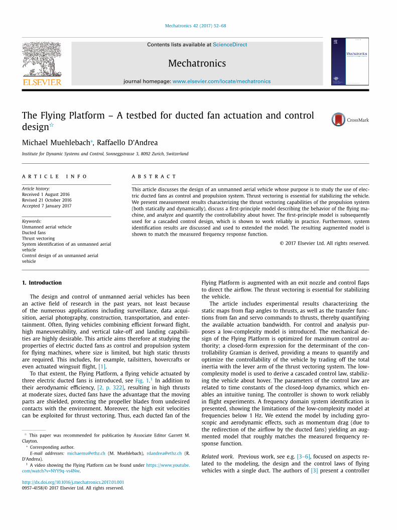
An actuation unit consists of an electric ducted fan, an outlet

ozzle, and two control flaps for thrust vectoring, see Fig. 2 .

The thrust is generated by the Schübeler DS-51-DIA HST electric

ucted fan driven by the brushless DC motor DSM4640-950. Ac-

ording to the datasheet of the manufacturer the ducted fan is op-

imized for high static thrust, yielding exit velocities up to 90 m/s.

his makes thrust vectoring particularly interesting, since the force

esulting from a redirection of the airflow is proportional to the

quare of the airflow velocity. The electric ducted fan is embedded

n a convergent exit nozzle, which has an inlet area of 6940 mm

2

54 M. Muehlebach, R. D’Andrea / Mechatronics 42 (2017) 52–68

Fig. 2. The different components of a single actuation unit.

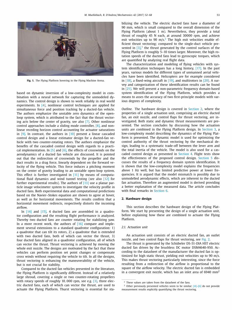
Fig. 3. Side and top view of control flap 2. The flap has 80 mm length (chord

length) and 83 mm width. Compared to the control flap 1, which has the same

dimensions and the same airfoil (NACA0015), a triangular part of control flap 2 is

cut out.

S

v

r

f

t

s

a

u

b

t

t

g

fi

i

a

o

p

s

p

t

m

n

i

1

o

c

t

m

T

b

m

t

s

m

t

a

and an outlet area of 5540 mm

2 . Thus, the cross section is reduced

by around 20% causing the airflow to accelerate through the noz-

zle. The motor controller (YGE 90HV) is mounted to the exit nozzle

and is cooled by the airflow. More precisely, the fins that are at-

tached to the motor controller are inserted in the airflow through

the hole in the exit nozzle, as shown in Fig. 2 . The hole in the exit

nozzle is designed such that the motor controller holds in place

(press fit). In addition, the outlet nozzle has a mount for the two

servos (Dynamixel RX-24F), where each servo actuates a control

flap. Both the outlet nozzle and the control flaps are 3D-printed in

ABS-M30. The roughness average characterizing the surface rough-

ness of the flaps and the exit nozzle is estimated to be around

R a = 3 . 2 μm. In [22] , the impact of roughness on the lift charac-

teristics of a NACA0015 airfoil is characterized. It is found that at

a Reynolds number of 220,0 0 0, which is comparable to our set-

up, an increased roughness would reduce the produced lift up to

40%. However, an increased roughness also delays the airfoil’s stall

to higher angles of attacks (up to a factor of two). In our case, the

flaps, which have likewise a NACA0015 profile, operate at relatively

high angles of attack, and therefore the roughness of the airfoil is

not necessarily a disadvantage, as it might prevent stall. Note that

the effect of roughness seems strongly influenced by the Reynolds

number and the specific airfoil. For example, the reduction of lift

due to roughness reported in [23] , where windtunnel tests with

the DU300-mod airfoil at Reynolds numbers above 3.6 × 10 6 are

presented, are less drastic.

The two control flaps are aligned orthogonally to simplify the

mechanical design of the actuation mechanism. To achieve an ac-

tuation radius of ± 18 ° for both flaps, a triangular part of con-

trol flap 2 is cut out, thereby reducing the maximum thrust devia-

tion achieved by control flap 2 approximately by a factor of two. A

chord length of 80 mm is chosen for both flaps. The choice of the

airfoil (NACA0015) is based on an optimization of the stall angle

with the XFoil software package 4 at a Reynolds number of 350,0 0 0,

corresponding to a typical airflow velocity of 70 m/s. 5

Characterization of a single actuation unit. The available thrust, and

the ability of the control flaps to vector thrust is characterized us-

ing force measurements with the transducer ATI Mini-40 using the

4 See http://web.mit.edu/drela/Public/web/xfoil/ . 5 The airflow velocity estimate is based on momentum theory, [2, p. 322, equa-

tion (6.41)] . For the calculation of the Reynolds number a temperature of 30 ° C is

assumed, which is motivated by the heat loss of the motor controller and the elec-

trical motor. The parameter Ncrit that describes the transition criterion in XFoil is

set to 7.

o

b

T

p

m

u

I-20-1 calibration. This results in a sensing range of ± 60 N in the

ertical direction and ± 20 N in the horizontal direction, with a

esolution of 0.01 N. The experimental results are presented in the

ollowing.

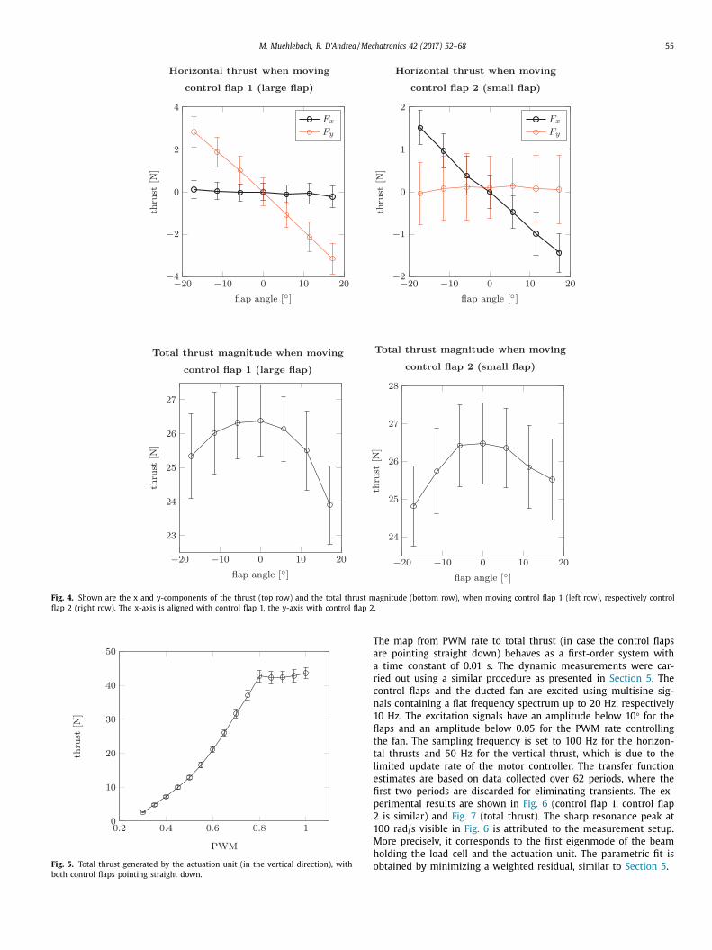
Static thrust measurements are shown in Fig. 4 . A single ac-

uation unit is attached to the load cell. The motorcontroller, the

ervos, and the load cell are interfaced using the PX4 flight man-

gement unit, [24] . The fan is run at a constant pulse-width mod-

lation (PWM) rate, resulting in a constant thrust of 26.4 N when

oth control flaps point straight down (this corresponds roughly

o the hover condition of the Flying Platform). Measurements are

aken at 7 different flap angles, which is found to be enough for

uaranteeing that the 68% confidence interval of a resulting linear

t is below 0.024 N/ ° (slope) and 0.27 N (offset). The flap angle

s set by the servo, which has a resolution of 0.29 °. For each flap

ngle, 500 measurement points are taken at a sampling frequency

f 50 Hz. The standard deviation obtained at each measurement

oint is indicated by the bars shown in Fig. 4 . The thrust mea-

urements display a relatively large standard deviation, which is

ossibly due to the turbulent flow in the exit nozzle induced by

he high Reynolds number, the roughness of the 3D print, and the

otor controller mount, but also due to a slight play in the con-

ection of the control flaps with the servos. Summarizing, a max-

mum horizontal thrust of 3 N can be generated by control flap

, whereas control flap 2 generates a maximum horizontal thrust

f 1.5 N. This is not unexpected, since compared to control flap 1,

ontrol flap 2 has roughly half the area available for deviating the

hrust. Moreover, if control flap is fully inclined, the total thrust

agnitude is reduced by around 2 N, as shown in Fig. 4 (bottom).

he decrease in total thrust is not entirely symmetric. This might

e caused by the motor controller mount that destroys the sym-

etry of the airflow through the exit nozzle.

Similar experiments are carried out for characterizing the total

hrust as a function of the PWM rate given to the motorcontroller,

ee Fig. 5 . The plateau that is visible above a duty cycle of 0.8 is

ost likely due to limitations of the motor controller. The rota-

ional speed of the ducted fan is found to be roughly constant at

fixed PWM rate, as can be inferred from current measurements

f a single motor phase. A linear fit through the data points neigh-

oring the PWM rate of 0.6 is performed, and will be used later.

he 68% confidence interval of the fit is 0.127 N/% for the linear

art and 0.7 N for the offset.

Dynamic measurements reveal that the flap angle to thrust

aps can be approximated by second-order systems, with a nat-

ral frequency of around 80 rad/s and a damping of roughly 0.4.

M. Muehlebach, R. D’Andrea / Mechatronics 42 (2017) 52–68 55

Fig. 4. Shown are the x and y-components of the thrust (top row) and the total thrust magnitude (bottom row), when moving control flap 1 (left row), respectively control

flap 2 (right row). The x-axis is aligned with control flap 1, the y-axis with control flap 2.

Fig. 5. Total thrust generated by the actuation unit (in the vertical direction), with

both control flaps pointing straight down.

T

a

a

r

c

n

1

fl

t

t

l

e

fi

p

2

1

M

h

o

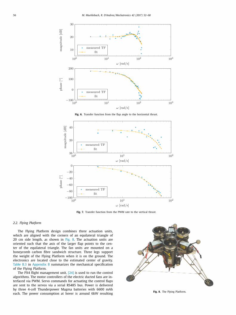
he map from PWM rate to total thrust (in case the control flaps

re pointing straight down) behaves as a first-order system with

time constant of 0.01 s. The dynamic measurements were car-

ied out using a similar procedure as presented in Section 5 . The

ontrol flaps and the ducted fan are excited using multisine sig-

als containing a flat frequency spectrum up to 20 Hz, respectively

0 Hz. The excitation signals have an amplitude below 10 ° for the

aps and an amplitude below 0.05 for the PWM rate controlling

he fan. The sampling frequency is set to 100 Hz for the horizon-

al thrusts and 50 Hz for the vertical thrust, which is due to the

imited update rate of the motor controller. The transfer function

stimates are based on data collected over 62 periods, where the

rst two periods are discarded for eliminating transients. The ex-

erimental results are shown in Fig. 6 (control flap 1, control flap

is similar) and Fig. 7 (total thrust). The sharp resonance peak at

00 rad/s visible in Fig. 6 is attributed to the measurement setup.

ore precisely, it corresponds to the first eigenmode of the beam

olding the load cell and the actuation unit. The parametric fit is

btained by minimizing a weighted residual, similar to Section 5 .

56 M. Muehlebach, R. D’Andrea / Mechatronics 42 (2017) 52–68

Fig. 6. Transfer function from the flap angle to the horizontal thrust.

Fig. 7. Transfer function from the PWM rate to the vertical thrust.

Fig. 8. The Flying Platform.

2.2. Flying Platform

The Flying Platform design combines three actuation units,

which are aligned with the corners of an equilateral triangle of

20 cm side length, as shown in Fig. 8 . The actuation units are

oriented such that the axis of the larger flap points to the cen-

ter of the equilateral triangle. The fan units are mounted on a

honeycomb carbon fibre sandwich structure. Three legs support

the weight of the Flying Platform when it is on the ground. The

electronics are located close to the estimated center of gravity.

Table B.3 in Appendix B summarizes the mechanical specification

of the Flying Platform.

The PX4 flight management unit, [24] is used to run the control

algorithms. The motor controllers of the electric ducted fans are in-

terfaced via PWM. Servo commands for actuating the control flaps

are sent to the servos via a serial RS485 bus. Power is delivered

by three 4-cell Thunderpower Magma batteries with 6600 mAh

each. The power consumption at hover is around 6kW resulting

M. Muehlebach, R. D’Andrea / Mechatronics 42 (2017) 52–68 57

I�ex

I�ey

B�ex

B�ey

S

S1 S2

S3

2�e x

2�e y

1 �ex

1 �ey

3�ex

3�ey

2 · l1Fig. 9. Schematic outline of the Flying Platform showing the coordinate frames { I }, { i }, i = 1 , 2 , 3 , and { B } (courtesy of Tobias Meier).

i

l

3

f

f

n

p

b

s

s

f

R

v

i

t

R

r

B

v

w

S

p

m

d

e

c

b

t

o

b

s

l

S

Si

�MTi

�Fi

�Λi

Si

�MTi

�Λi

i�ez

Oi

i�ex

l3

Fig. 10. Free body diagram of a single actuation unit (courtesy of Tobias Meier). The

motor torque � M Ti is aligned with the z-axis of the local coordinate frame { i }. The

vertical thrust, as well as the horizontal thrust generated by the two the control

flaps are combined in the force � F i .

t

�

m

C

w

i

d

T

w

t

t

d

v

n a flight time of around 3 min. The batteries weigh 680 g each,

eading to a total weight of the Flying Platform of 8.0 kg.

. Dynamics

This section presents a low-complexity model of the Flying Plat-

orm. The nonlinear equations of motion are linearized about hover

or control and analysis purposes. We will optimize the determi-

ant of the controllability Gramian as a function of the actuator

lacements and thereby maximize the controllability about hover.

Notation. We introduce an inertial coordinate system { I } , a

ody-fixed coordinate system { B } , and local body-fixed coordinate

ystems { i } oriented along the control flaps of the actuation units,

ee Fig. 9 . The projection of a tensor onto a particular coordinate

rame is denoted by a preceding superscript, i.e. B � ∈ R

3 ×3 , B F ∈

3 . The arrow notation, e.g. in Fig. 9 , is used to emphasize that a

ector (and tensor) should be a priori thought of as a linear object

n a normed vector space detached from its coordinate represen-

ation in a particular coordinate frame. The transformation matrix

IB ∈ SO (3) relates vectors from the body-fixed frame to their rep-

esentation in the inertial frame, that is I v = R IB B v , for all vectors

v ∈ R

3 . Moreover, the skew symmetric matrix corresponding to a

ector a ∈ R

3 , denoted by a , is defined as a × b =

a b, for all b ∈ R

3 ,

here a × b refers to the cross product of the two vectors a and b .

ince the body-fixed coordinate frame { B } is the most commonly

rojected coordinate frame, its preceding superscript is usually re-

oved for ease of notation, that is, B m = m, B � = �, etc. The stan-

ard unit vectors in R

3 are denoted by e x , e y , and e z . Vectors are

xpressed as n -tuples (x 1 , x 2 , . . . , x n ) with dimension and stacking

lear from the context.

Dynamics. The equations of motion can be derived, for example,

y using the principle of virtual power, [25, Ch. 3] . To that extent,

he moving parts of the i th actuation unit (turbine blades and shaft

f the electrical motor) are separated from the remaining structure

y introducing the constraint forces � �i and the motor torques �

M T i ,

ee Fig. 10 . Requiring the virtual power to vanish for all virtual ve-

ocities (translational and rotational) yields the following charac-

erization of the dynamic equilibrium,

˙ ω +

3 ∑

i =1

�i ˙ ω i = −˜ ω

(

�ω +

3 ∑

i =1

�i ω i

)

+

3 ∑

i =1

r i F i , (1)

I ˙ v = m

I g +

3 ∑

i =1

R IB F i , (2)

e T z ( ˙ ω + ˙ ω i ) = M i , i = 1 , 2 , 3 , (3)

here � denotes the total inertia of the Flying Platform referred to

ts center of gravity S , �i the inertia of the moving parts of the i th

ucted fan referred to its center of rotation, and m the total mass.

he velocity of the center of mass of the vehicle is denoted by v ,hereas ω refers to its angular velocity, i.e. the angular velocity of

he frame { B } with respect to frame { I }. The thrust generated by

he i th actuation unit, that is, the vertical thrust from the electric

ucted fan, vectored by the two control flaps, is denoted by F i . The

ector from the center of gravity to the point of origin of the force

58 M. Muehlebach, R. D’Andrea / Mechatronics 42 (2017) 52–68

V

L

l

b

t

M

b

d

c

u

w

b

e

t

t

t

E

m

c

R

F

t

c

t

a

t

R

a

m

w

f

a

J

w

r

s

ω

F

l

d

f

s

�

T

o

F i is denoted by r i . Aerodynamic effects except the forces gener-

ated by the control flaps and the thrust of the fans are neglected.

These will be included in an augmented model as presented in

Section 5 . The scalar M i and the vector ω i denote the torque of the

electrical motor, respectively the angular rate (relative to the body-

fixed frame { B }) of the i th ducted fan. The rotating parts (turbine

blades and electrical motor) of the actuation units are assumed to

be symmetric and rotate about their respective center of gravity

resulting in

6

�i =: diag ( C , C , C) . (4)

The angular velocity vector ω i is assumed to have only a compo-

nent along the z-axis of the body-fixed frame. Therefore its rate

of change ˙ ω i appearing in (1) can be eliminated with (3) resulting

in

ˆ � ˙ ω = −˜ ω

(

�ω +

3 ∑

i =1

�i ω i

)

+

3 ∑

i =1

( r i F i − e z M i ) , (5)

where

ˆ � := � − 3 C e z e T z . (6)

We will consider the thrusts generated by the actuation units

and expressed in their local coordinate frames { i } to be the in-

puts to the system. The servo and PWM-commands for the elec-

tric ducted fans are then calculated by inverting the linearization

of the static maps presented in Section 2.1 . The total thrust and

the resulting torque are linear in the thrusts generated by the ac-

tuation units (the inputs), more precisely,

3 ∑

i =1

F i = T 1 u,

3 ∑

i =3

r i F i = T 2 u, (7)

where u := ( 1 F 1 , 2 F 2 ,

3 F 3 ) ,

T 1 :=

(T 11

T 12

), T 2 :=

(T 21

T 22

), (8)

with

T 11 :=

(1 0 0 −1 / 2 −√

3 / 2 0 −1 / 2

√

3 / 2 0

0 1 0

√

3 / 2 −1 / 2 0 −√

3 / 2 −1 / 2 0

), (9)

T 12 :=

(0 0 1 0 0 1 0 0 1

), (10)

T 21 := l 3 JT 11 + 2

√

3 / 3 l 1 V 1 , (11)

T 22 := −2

√

3 / 3 l 1 (0 1 0 0 1 0 0 1 0

), (12)

1 :=

(0 0 0 0 0 −√

3 / 2 0 0

√

3 / 2

0 0 1 0 0 −1 / 2 0 0 −1 / 2

), (13)

J :=

(0 1

−1 0

). (14)

As a result, the evolution of the center of gravity and the evolution

of the angular velocity are given by

m

I ˙ v = m

I g + R IB T 1 u, (15)

ˆ � ˙ ω = −˜ ω

(

�ω +

3 ∑

i =1

�i ω i

)

+ T 2 u − e z

3 ∑

i =1

M i . (16)

6 In fact, the expression remains unchanged if the inertia is expressed in the local

frame { i } or in a frame attached to the moving parts of fan i (as long as the z-axes

are aligned).

o

i

r(

inearization. For control and analysis purposes the dynamics are

inearized about hover. The three ducted fans are assumed to

e identical and to rotate in the same direction. Thus, at hover,

he torques M i have the same values, that is, M i = M, i = 1 , 2 , 3 .

oreover, the torques M and the weight of the vehicle must

e balanced by the thrust generated by the ducted fans and

eviated by the control flaps, which is achieved by the thrust

ommand

¯ := ( 0 , −M

√

3 / (2 l 1 ) , mg 0 / 3 ,

0 , −M

√

3 / (2 l 1 ) , mg 0 / 3 ,

0 , −M

√

3 / (2 l 1 ) , mg 0 / 3) ,

here g 0 := 9.81 m/s 2 denotes the gravitational acceleration. For

etter readability the components of the vector u in the above

quation are grouped according to the different actuation units,

hat is, the first line contains the x, y, and z-components of the

hrust assigned to the first fan unit, the second line contains the

hrust assigned to the second fan unit, etc. We further introduce

uler angles ( α, β , γ ) (roll, pitch, yaw) to parametrize the rotation

atrix R IB . Using the matrix exponential, the rotation matrix R IB an be expressed as

IB = e e z γ e e y βe e x α. (17)

or control purposes it will be convenient to obtain a linearization

hat is invariant to yaw. Therefore the position and velocity of the

enter of gravity will be expressed in a separate coordinate sys-

em { J } obtained by rotating the inertial system { I } about I � e z by the

ngle γ . Hence, the rotation matrix R IB is decomposed according

o

IB = R IJ R JB , R IJ = e e z γ , R JB = e e y βe e x α, (18)

nd (15) is reformulated as

J ˙ v = −m γ e z × J v + m

J g + R JB T 1 u, (19)

here the convective derivative enters due to the fact that the

rame { J } is non-inertial. Linearizing the translational dynamics

round hover, i.e. J v = 0 , R JB = I, ω = 0 , yields

˙ v ≈ −α˜ e x J g − β˜ e y

J g +

1

m

T 1 (u − u ) (20)

= g 0 ( α˜ e x e z + β˜ e y e z ) +

1

m

T 1 (u − u ) (21)

= g 0 ( −e y α + e x β) +

1

m

T 1 (u − u ) , (22)

hich holds independent of the angle γ . Similarly, linearizing the

otational dynamics (16) around ω = 0 , and neglecting the gyro-

copic term C �−1 ˜ ω ω i results in

˙ ≈ ˆ �−1 T 2 u − ˆ �−1 e z

3 ∑

i =1

M i . (23)

rom (22) and (23) it can be inferred that the poles of the open-

oop system all lie at 0, and that the height and yaw dynamics are

ecoupled from the x, y, and roll and pitch dynamics.

Assuming further that the mass distribution of the Flying Plat-

orm has a three-fold rotational symmetry about its figure axis B � e z

implifies the inertia tensor ˆ � to

ˆ =: diag (I 1 , I 1 , I 3 ) . (24)

his is a reasonable assumption due to the symmetric placement

f both the actuation units and the batteries, and the symmetry

f the frame, which together constitute the main mass of the Fly-

ng Platform. Thus, the x, y, and roll and pitch dynamics can be

ewritten as

˙ v x ˙ v y

)≈ g 0 J

(αβ

)+

1

m

T 11 (u − u ) ,

(α

β

)≈ 1

I 1 T 21 (u − u ) , (25)

M. Muehlebach, R. D’Andrea / Mechatronics 42 (2017) 52–68 59

w

v

C

F

t

(

f

fi

n

t

i

s

b

t

x

t

d

x

f

W

T

A

s

i

W

T

m

c

d

T

l

p

m

a

I

w

t

t

p

FPpos, vel, att

des pos ωdes

ωservo andthrust cmds

offboardcomputer

onboardcomputer

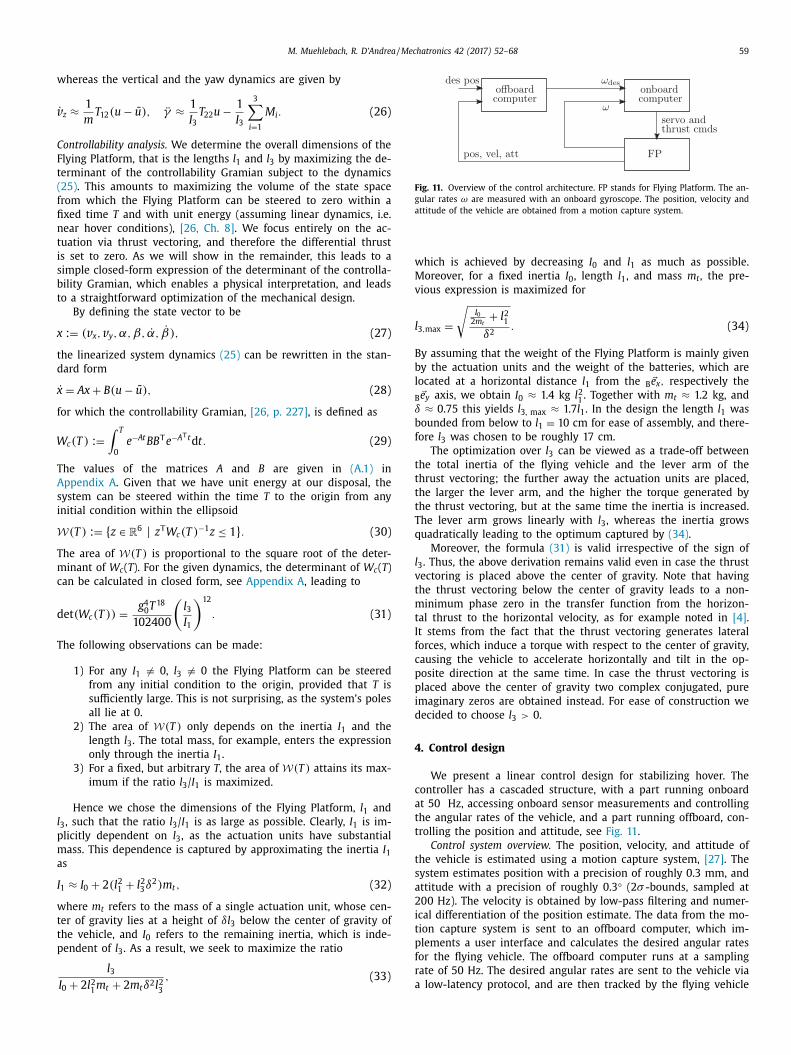
Fig. 11. Overview of the control architecture. FP stands for Flying Platform. The an-

gular rates ω are measured with an onboard gyroscope. The position, velocity and

attitude of the vehicle are obtained from a motion capture system.

w

M

v

l

B

b

l

B

δ

b

f

t

t

t

t

T

q

l

v

t

m

t

I

f

c

p

p

i

d

4

c

a

t

t

t

s

a

2

i

t

p

f

r

a

hereas the vertical and the yaw dynamics are given by

˙ z ≈ 1

m

T 12 (u − u ) , γ ≈ 1

I 3 T 22 u − 1

I 3

3 ∑

i =1

M i . (26)

ontrollability analysis. We determine the overall dimensions of the

lying Platform, that is the lengths l 1 and l 3 by maximizing the de-

erminant of the controllability Gramian subject to the dynamics

25) . This amounts to maximizing the volume of the state space

rom which the Flying Platform can be steered to zero within a

xed time T and with unit energy (assuming linear dynamics, i.e.

ear hover conditions), [26, Ch. 8] . We focus entirely on the ac-

uation via thrust vectoring, and therefore the differential thrust

s set to zero. As we will show in the remainder, this leads to a

imple closed-form expression of the determinant of the controlla-

ility Gramian, which enables a physical interpretation, and leads

o a straightforward optimization of the mechanical design.

By defining the state vector to be

:= (v x , v y , α, β, ˙ α, ˙ β) , (27)

he linearized system dynamics (25) can be rewritten in the stan-

ard form

˙ = Ax + B (u − u ) , (28)

or which the controllability Gramian, [26, p. 227] , is defined as

c (T ) :=

∫ T

0

e −At BB

T e −A T t d t. (29)

he values of the matrices A and B are given in (A.1) in

ppendix A . Given that we have unit energy at our disposal, the

ystem can be steered within the time T to the origin from any

nitial condition within the ellipsoid

(T ) := { z ∈ R

6 | z T W c (T ) −1 z ≤ 1 } . (30)

he area of W(T ) is proportional to the square root of the deter-

inant of W c ( T ). For the given dynamics, the determinant of W c ( T )

an be calculated in closed form, see Appendix A , leading to

et (W c (T )) =

g 4 0 T 18

102400

(l 3 I 1

)12

. (31)

he following observations can be made:

1) For any I 1 � = 0, l 3 � = 0 the Flying Platform can be steered

from any initial condition to the origin, provided that T is

sufficiently large. This is not surprising, as the system’s poles

all lie at 0.

2) The area of W(T ) only depends on the inertia I 1 and the

length l 3 . The total mass, for example, enters the expression

only through the inertia I 1 .

3) For a fixed, but arbitrary T , the area of W(T ) attains its max-

imum if the ratio l 3 / I 1 is maximized.

Hence we chose the dimensions of the Flying Platform, l 1 and

3 , such that the ratio l 3 / I 1 is as large as possible. Clearly, I 1 is im-

licitly dependent on l 3 , as the actuation units have substantial

ass. This dependence is captured by approximating the inertia I 1 s

1 ≈ I 0 + 2(l 2 1 + l 2 3 δ2 ) m t , (32)

here m t refers to the mass of a single actuation unit, whose cen-

er of gravity lies at a height of δl 3 below the center of gravity of

he vehicle, and I 0 refers to the remaining inertia, which is inde-

endent of l 3 . As a result, we seek to maximize the ratio

l 3

I 0 + 2 l 2 1

m t + 2 m t δ2 l 2 3

, (33)

hich is achieved by decreasing I 0 and l 1 as much as possible.

oreover, for a fixed inertia I 0 , length l 1 , and mass m t , the pre-

ious expression is maximized for

3 , max =

√

I 0 2 m t

+ l 2 1

δ2 . (34)

y assuming that the weight of the Flying Platform is mainly given

y the actuation units and the weight of the batteries, which are

ocated at a horizontal distance l 1 from the B � e x , respectively the

� e y axis, we obtain I 0 ≈ 1.4 kg l 2

1 . Together with m t ≈ 1.2 kg, and

≈ 0.75 this yields l 3, max ≈ 1.7 l 1 . In the design the length l 1 was

ounded from below to l 1 = 10 cm for ease of assembly, and there-

ore l 3 was chosen to be roughly 17 cm.

The optimization over l 3 can be viewed as a trade-off between

he total inertia of the flying vehicle and the lever arm of the

hrust vectoring; the further away the actuation units are placed,

he larger the lever arm, and the higher the torque generated by

he thrust vectoring, but at the same time the inertia is increased.

he lever arm grows linearly with l 3 , whereas the inertia grows

uadratically leading to the optimum captured by (34) .

Moreover, the formula (31) is valid irrespective of the sign of

3 . Thus, the above derivation remains valid even in case the thrust

ectoring is placed above the center of gravity. Note that having

he thrust vectoring below the center of gravity leads to a non-

inimum phase zero in the transfer function from the horizon-

al thrust to the horizontal velocity, as for example noted in [4] .

t stems from the fact that the thrust vectoring generates lateral

orces, which induce a torque with respect to the center of gravity,

ausing the vehicle to accelerate horizontally and tilt in the op-

osite direction at the same time. In case the thrust vectoring is

laced above the center of gravity two complex conjugated, pure

maginary zeros are obtained instead. For ease of construction we

ecided to choose l 3 > 0.

. Control design

We present a linear control design for stabilizing hover. The

ontroller has a cascaded structure, with a part running onboard

t 50 Hz, accessing onboard sensor measurements and controlling

he angular rates of the vehicle, and a part running offboard, con-

rolling the position and attitude, see Fig. 11 .

Control system overview. The position, velocity, and attitude of

he vehicle is estimated using a motion capture system, [27] . The

ystem estimates position with a precision of roughly 0.3 mm, and

ttitude with a precision of roughly 0.3 ° (2 σ -bounds, sampled at

00 Hz). The velocity is obtained by low-pass filtering and numer-

cal differentiation of the position estimate. The data from the mo-

ion capture system is sent to an offboard computer, which im-

lements a user interface and calculates the desired angular rates

or the flying vehicle. The offboard computer runs at a sampling

ate of 50 Hz. The desired angular rates are sent to the vehicle via

low-latency protocol, and are then tracked by the flying vehicle

60 M. Muehlebach, R. D’Andrea / Mechatronics 42 (2017) 52–68

Table 1

Root-mean-squared errors when hovering in

steady state.

rms error (x,y,z component)

I r 0.013 m 0.029 m 0.005 m

φ 0 .007 ° 0 .004 ° 0 .008 °ω 0.029 rad/s 0.022 rad/s 0.011 rad/s

d

ω

l

t

b

i

s

[

i

w

s

c

i

t

5

p

S

t

t

e

p

h

t

t

t

w

i

w

g

o

1

P

o

b

a

F

R

w

c

s

m

i

p

f

o

λ

a

n

p

using the gyroscope included on the PX4 flight computer. The on-

board control algorithm runs at 50 Hz. Telemetry data from the

flying vehicle is sent out via a separate wireless radio.

Onboard control. The onboard controller tracks the desired an-

gular rates ω des , which are obtained from the offboard computer.

About hover, the rotational dynamics can be approximated by, c.f.

(23) ,

˙ ω =

ˆ �−1 T 2 (u − u ) , (35)

where the torques M i are approximated as constants, compensated

by the steady-state control input u . A linear quadratic regulator,

with state weight 512 · I and input weight

diag ( 1 , 2 , 2 , ︸ ︷︷ ︸ 1st actuation unit x,y,z-components

1 , 2 , 2 , ︸ ︷︷ ︸ 2nd actuation unit x,y,z-components

1 , 2 , 2 ︸ ︷︷ ︸ 3rd actuation unit x,y,z-components

) (36)

is used to compute a constant feedback gain K , rendering

(35) asymptotically stable with

u = u − K(ω − ω des ) + (0 , 0 , 1 , 0 , 0 , 1 , 0 , 0 , 1) F z , (37)

where F z denotes the collective thrust of the three electric ducted

fans. The collective thrust does not affect the angular rates and will

be used in a later stage to control the height of the flying vehicle.

The obtained feedback gain K results in closed-loop poles at 42

rad/s (for ω x ), 42 rad/s (for ω y ), and 25 rad/s (for ω z ).

Offboard control. Under the assumption that the inner control

loop has a substantially faster time constant, we consider ω des

to be the control input of the outer control loop, controlling the

position, attitude, and velocity of the flying vehicle. As a result,

(22) simplifies to

˙ v x ≈ βg 0 , ˙ v y ≈ −αg 0 , ˙ v z =

3

m

F z , (38)

where J v =: (v x , v y , v z ) . Differentiating the first two equations with

respect to time yields

v x = ω des ,y g 0 , v y = −ω des ,x g 0 . (39)

Thus we choose

ω des ,x =

1

g 0 ( −(2 d y w y + p y ) g 0 α

+(w

2 y + 2 d y w y p y ) v y + p y w

2 y (y − y des )

), (40)

ω des ,y =

1

g 0 ( −(2 d x w x + p x ) g 0 β

−(w

2 x + 2 d x w x p x ) v x − p x w

2 x (x − x des )

), (41)

ω des ,z = − 1

g 0 p z (γ − γdes ) , (42)

F z =

m

3

(−2 d z w z v z − w

2 z (z − z des )) , (43)

where d i , w i , p i with i = x, y, z are constants, x , y , z and

x des , y des , z des denotes the actual and desired position of the ve-

hicle expressed in the { J } frame, and γ des the desired yaw an-

gle. The constants d i , w i , p i with i = x, y are chosen such that the

translational closed-loop dynamics in the { J } frame result in two

decoupled third-order systems with one pole located at −p x (re-

spectively −p y ) and a remaining second-order system with damp-

ing d x (respectively d y ) and natural frequency w x (respectively w y ).

The constant p z determines the time-constant of the yaw dynam-

ics, whereas the closed-loop dynamics for the height result in a

second-order system with damping d z and natural frequency w z .

The constants are set to the following values

x = d y = d z = 1 ,

x = ω y = 3 rad/s , ω z = 2 rad/s ,

p x = p y = 1 rad/s , p z = 2 rad/s ,

eading to a clear separation of the time constants associated with

he inner and the outer control loop. This results in a symmetric

ehavior in the x and y-directions, whereas the height is controlled

n a slightly less aggressive manner ( ω z < ω x , ω y ). The damping is

et to 1, leading to critically damped systems.

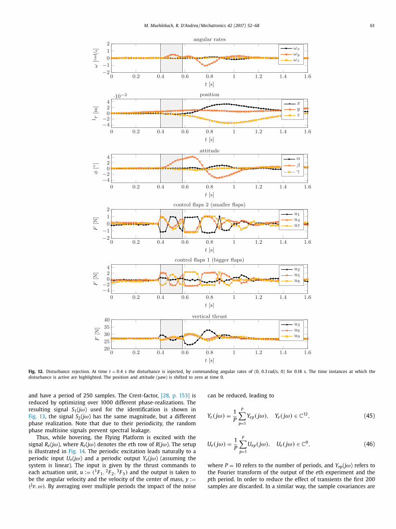
Flight experiments are carried out in the Flying Machine Arena,

27] . Table 1 shows the root-mean-squared errors when hovering

n steady state. It follows that the vehicle maintains its position

ithin a few centimeters. Disturbance rejection measurements are

hown in Fig. 12 . The disturbance is generated by commanding a

onstant angular rate in y -direction, ω y = 0 . 3 rad/s for 0.18 s, lead-

ng to a pitch of approximately 4 ° from which the vehicle is able

o recover.

. System identification

The following section describes a frequency domain-based ap-

roach for identifying the parameters of the Flying Platform.

pecifically, the aim is to quantify the model quality and identify

he matrices T 1 / m and

ˆ �−1 T 2 , essentially determining the rota-

ional and translational dynamics, (15) and (16) . This is done by

xciting the system while hovering with periodic, sinusoidal in-

uts, and measuring its reaction. Due to the fact that the system

as nine inputs defined as the thrust commands of each actua-

ion unit, at least nine different experiments are used to measure

he corresponding frequency response function. In order to reduce

he noise influence we performed in total 18 different experiments,

hich are based on two different excitation signals (for increas-

ng robustness against nonlinearities, [28, Ch. 3] ). The experiments,

hich are referred to by the subscript e , e ∈ { 1 , 2 , . . . , 18 } , can be

rouped in three parts: Part 1) ( e ∈ {1, 4, 7, 10, 13, 16}): excitation

f the control flaps 1 of each actuation unit; Part 2) ( e ∈ {2, 5, 8,

1, 14, 17}): excitation of the control flaps 2 of each actuation unit;

art 3) ( e ∈ {3, 6, 9, 12, 15, 18}): excitation of the vertical thrusts

f each actuation unit. The different excitation signals are obtained

y multiplying two scalar random phase multisine signals S 1 ( j ω)

nd S 2 ( j ω) (to be made precise below) with the 3-point discrete

ourier transform matrix V ( jω) ∈ C

3 ×3 , resulting in

( jω) =

(( V ( jω) � diag (λ) ) S 1 ( jω) ( V ( jω) � diag (λ) ) S 2 ( jω)

), R ( jω) ∈ C

18 ×9 , (44)

here λ ∈ R

3 , λ > 0 represents a positive gain for scaling the ex-

itation, and � refers to the Kronecker product. Multiplying the

calar multisine signals with the 3-point discrete Fourier transform

atrix leads to an improved condition number of the pseudo-

nverse needed to calculate the frequency response function, [28,

. 66] . The matrix R ( j ω) contains the excitation signals for the dif-

erent inputs as rows. Hence, for example in the first experiment

f Part 1), the excitation signals λ1 V 11 ( j ω) S 1 ( j ω), λ1 V 12 ( j ω) S 1 ( j ω),

1 V 13 ( j ω) S 1 ( j ω) are used to excite the control flaps 1 of each actu-

tion unit (the remaining control flaps and the vertical thrusts are

ot excited). The multisine signals S 1 ( j ω) and S 2 ( j ω) have a random

hase uniformly distributed in [0, 2 π ), are sampled with 50 Hz,

M. Muehlebach, R. D’Andrea / Mechatronics 42 (2017) 52–68 61

Fig. 12. Disturbance rejection. At time t = 0 . 4 s the disturbance is injected, by commanding angular rates of (0, 0.3 rad/s, 0) for 0.18 s. The time instances at which the

disturbance is active are highlighted. The position and attitude (yaw) is shifted to zero at time 0.

a

r

r

F

p

p

s

i

p

s

e

b

c

Y

U

w

t

p

s

nd have a period of 250 samples. The Crest-factor, [28, p. 153] is

educed by optimizing over 10 0 0 different phase-realizations. The

esulting signal S 1 ( j ω) used for the identification is shown in

ig. 13 , the signal S 2 ( j ω) has the same magnitude, but a different

hase realization. Note that due to their periodicity, the random

hase multisine signals prevent spectral leakage.

Thus, while hovering, the Flying Platform is excited with the

ignal R e ( j ω), where R e ( j ω) denotes the e th row of R ( j ω). The setup

s illustrated in Fig. 14 . The periodic excitation leads naturally to a

eriodic input U e ( j ω) and a periodic output Y e ( j ω) (assuming the

ystem is linear). The input is given by the thrust commands to

ach actuation unit, u := ( 1 F 1 , 2 F 2 ,

3 F 3 ) and the output is taken to

e the angular velocity and the velocity of the center of mass, y :=( J v , ω) . By averaging over multiple periods the impact of the noise

an be reduced, leading to

e ( jω) =

1

P

P ∑

p=1

Y ep ( jω) , Y e ( jω) ∈ C

12 , (45)

e ( jω) =

1

P

P ∑

p=1

U ep ( jω) , U e ( jω) ∈ C

9 , (46)

here P = 10 refers to the number of periods, and Y ep ( j ω) refers to

he Fourier transform of the output of the e th experiment and the

th period. In order to reduce the effect of transients the first 200

amples are discarded. In a similar way, the sample covariances are

62 M. Muehlebach, R. D’Andrea / Mechatronics 42 (2017) 52–68

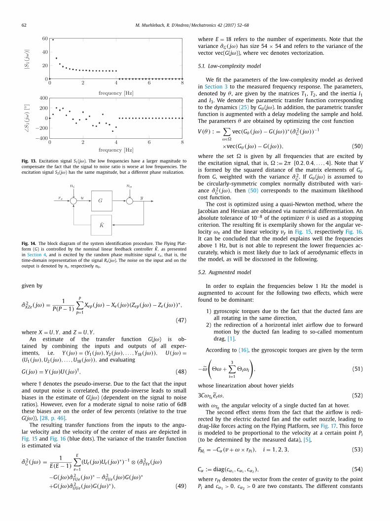
Fig. 13. Excitation signal S 1 ( j ω). The low frequencies have a larger magnitude to

compensate the fact that the signal to noise ratio is worse at low frequencies. The

excitation signal S 2 ( j ω) has the same magnitude, but a different phase realization.

Fig. 14. The block diagram of the system identification procedure. The Flying Plat-

form ( G ) is controlled by the nominal linear feedback controller K , as presented

in Section 4 , and is excited by the random phase multisine signal r e , that is, the

time-domain representation of the signal R e ( j ω). The noise on the input and on the

output is denoted by n i , respectively n 0 .

w

v

v

5

i

d

a

t

f

T

V

w

t

i

f

b

a

c

J

a

c

l

I

a

c

t

5

a

f

−

w

3

w

r

d

i

(

F

C

w

P

given by

ˆ σ 2 XZe ( jω) =

1

P (P − 1)

P ∑

p=1

X ep ( jω) − X e ( jω)(Z ep ( jω) − Z e ( jω)) ∗,

(47)

where X = U, Y, and Z = U, Y .

An estimate of the transfer function G ( j ω) is ob-

tained by combining the inputs and outputs of all exper-

iments, i.e. Y ( jω) = (Y 1 ( jω) , Y 2 ( j ω) , . . . , Y 18 ( j ω)) , U( j ω) =(U 1 ( jω) , U 2 ( jω) , . . . , U 18 ( jω)) , and evaluating

G ( jω) = Y ( j ω) U( j ω) † , (48)

where † denotes the pseudo-inverse. Due to the fact that the input

and output noise is correlated, the pseudo-inverse leads to small

biases in the estimate of G ( j ω) (dependent on the signal to noise

ratios). However, even for a moderate signal to noise ratio of 6dB

these biases are on the order of few percents (relative to the true

G ( j ω)), [28, p. 46] .

The resulting transfer functions from the inputs to the angu-

lar velocity and the velocity of the center of mass are depicted in

Fig. 15 and Fig. 16 (blue dots). The variance of the transfer function

is estimated via

ˆ σ 2 G ( jω) =

1

E(E − 1)

E ∑

e =1

(U e ( jω) U e ( jω) ∗) −1 � ( σ 2

Y Ye ( jω)

−G ( jω) σ 2 Y Ue ( jω) ∗ − ˆ σ 2

Y Ue ( jω) G ( jω) ∗

+ G ( jω) σ 2 U U e ( jω) G ( jω) ∗) , (49)

here E = 18 refers to the number of experiments. Note that the

ariance ˆ σG ( jω) has size 54 × 54 and refers to the variance of the

ector vec( G ( j ω)), where vec denotes vectorization.

.1. Low-complexity model

We fit the parameters of the low-complexity model as derived

n Section 3 to the measured frequency response. The parameters,

enoted by θ , are given by the matrices T 1 , T 2 , and the inertia I 1 nd I 3 . We denote the parametric transfer function corresponding

o the dynamics (25) by G θ ( j ω). In addition, the parametric transfer

unction is augmented with a delay modeling the sample and hold.

he parameters θ are obtained by optimizing the cost function

(θ ) : =

∑

ω∈ �vec (G θ ( jω) − G ( jω)) ∗( σ 2

G ( jω)) −1

×vec (G θ ( jω) − G ( jω)) , (50)

here the set � is given by all frequencies that are excited by

he excitation signal, that is, � := 2 π { 0 . 2 , 0 . 4 , . . . , 4 } . Note that V

s formed by the squared distance of the matrix elements of G θ

rom G , weighted with the variance ˆ σ 2 G

. If G θ ( j ω) is assumed to

e circularly-symmetric complex normally distributed with vari-

nce ˆ σ 2 G ( jω) , then (50) corresponds to the maximum likelihood

ost function.

The cost is optimized using a quasi-Newton method, where the

acobian and Hessian are obtained via numerical differentiation. An

bsolute tolerance of 10 −8 of the optimizer θ is used as a stopping

riterion. The resulting fit is exemplarily shown for the angular ve-

ocity ω x and the linear velocity v y in Fig. 15 , respectively Fig. 16 .

t can be concluded that the model explains well the frequencies

bove 1 Hz, but is not able to represent the lower frequencies ac-

urately, which is most likely due to lack of aerodynamic effects in

he model, as will be discussed in the following.

.2. Augmented model

In order to explain the frequencies below 1 Hz the model is

ugmented to account for the following two effects, which were

ound to be dominant:

1) gyroscopic torques due to the fact that the ducted fans are

all rotating in the same direction,

2) the redirection of a horizontal inlet airflow due to forward

motion by the ducted fan leading to so-called momentum

drag, [1] .

According to (16) , the gyroscopic torques are given by the term

˜ ω

(

�ω +

3 ∑

i =1

�i ω i

)

, (51)

hose linearization about hover yields

Cω T 0 e z ω, (52)

ith ω T 0 the angular velocity of a single ducted fan at hover.

The second effect stems from the fact that the airflow is redi-

ected by the electric ducted fan and the outlet nozzle, leading to

rag-like forces acting on the Flying Platform, see Fig. 17 . This force

s modeled to be proportional to the velocity at a certain point P i to be determined by the measured data), [5] ,

M i = −C α(v + ω × r Pi ) , i = 1 , 2 , 3 , (53)

α := diag (c α1 , c α1

, c α2 ) , (54)

here r Pi denotes the vector from the center of gravity to the point

i and c α > 0 , c α > 0 are two constants. The different constants

1 2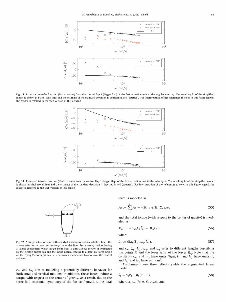

M. Muehlebach, R. D’Andrea / Mechatronics 42 (2017) 52–68 63

Fig. 15. Estimated transfer function (black crosses) from the control flap 1 (bigger flap) of the first actuation unit to the angular rates ω x . The resulting fit of the simplified

model is shown in black (solid line) and the estimate of the standard deviation is depicted in red (squares). (For interpretation of the references to color in this figure legend,

the reader is referred to the web version of this article.)

Fig. 16. Estimated transfer function (black crosses) from the control flap 1 (bigger flap) of the first actuation unit to the velocity v y . The resulting fit of the simplified model

is shown in black (solid line) and the estimate of the standard deviation is depicted in red (squares). (For interpretation of the references to color in this figure legend, the

reader is referred to the web version of this article.)

Fig. 17. A single actuation unit with a body-fixed control volume (dashed line). The

arrows refer to the inlet, respectively the outlet flow. An incoming airflow having

a lateral component, which might stem from a translational motion is redirected

by the electric ducted fan and the outlet nozzle, leading to a drag-like force acting

on the Flying Platform (as can be seen from a momentum balance over the control

volume).

c

h

t

t

f

F

a

e

M

w

L

a

t

c

a

m

x

w

α1 and c α2

aim at modeling a potentially different behavior for

orizontal and vertical motions. In addition, these forces induce a

orque with respect to the center of gravity. As a result, due to the

hree-fold rotational symmetry of the fan configuration, the total

orce is modeled as

M

:=

3 ∑

i =1

F M i = −3 C αv + 3 l α1

C α˜ e z ω, (55)

nd the total torque (with respect to the center of gravity) is mod-

led as

M

:= −3 l α2 C α˜ e z v − 3 L αC αω, (56)

here

α := diag (l α3 , l α3

, l α4 ) , (57)

nd c α , l α1 , l α2

, l α3 , and l α4

refer to different lengths describing

he points P i and the lever arms of the forces F M i . Note that the

onstants c α1 and c α2

have units Ns/m, l α1 and l α2

have units m,

nd l α3 and l α4

have units m

2 .

Combining these three effects yields the augmented linear

odel

˙ a = A a x a + B a (u − u ) , (58)

here x a := ( J v , α, β, γ , ω) , and

64 M. Muehlebach, R. D’Andrea / Mechatronics 42 (2017) 52–68

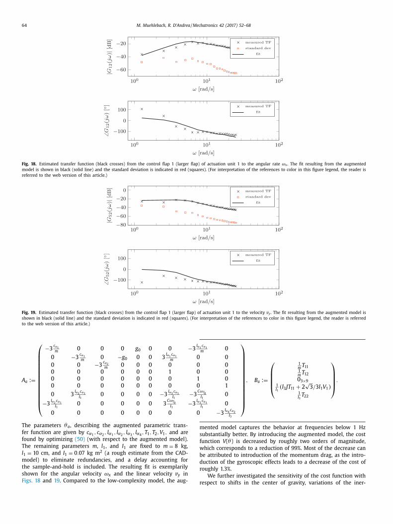
Fig. 18. Estimated transfer function (black crosses) from the control flap 1 (larger flap) of actuation unit 1 to the angular rate ω x . The fit resulting from the augmented

model is shown in black (solid line) and the standard deviation is indicated in red (squares). (For interpretation of the references to color in this figure legend, the reader is

referred to the web version of this article.)

Fig. 19. Estimated transfer function (black crosses) from the control flap 1 (larger flap) of actuation unit 1 to the velocity v y . The fit resulting from the augmented model is

shown in black (solid line) and the standard deviation is indicated in red (squares). (For interpretation of the references to color in this figure legend, the reader is referred

to the web version of this article.)

−3

l α1

0

0010

−3

C

−3

l α3

0

m

s

f

w

b

d

r

A a :=

⎛ ⎜ ⎜ ⎜ ⎜ ⎜ ⎜ ⎜ ⎜ ⎜ ⎜ ⎜ ⎜ ⎝

−3

c α1

m

0 0 0 g 0 0 0

0 −3

c α1

m

0 −g 0 0 0 3

l α1 c α1

m

0 0 −3

c α2

m

0 0 0 0

0 0 0 0 0 0 1

0 0 0 0 0 0 0

0 0 0 0 0 0 0

0 3

l α2 c α1

I 1 0 0 0 0 −3

l α3 c α1

I 1

−3

l α2 c α1

I 1 0 0 0 0 0 3

Cω T 0 I 1

0 0 0 0 0 0 0

The parameters θ a , describing the augmented parametric trans-

fer function are given by c α1 , c α2

, l α1 , l α2

, l α3 , l α4

, T 1 , T 2 , V 1 , and are

found by optimizing (50) (with respect to the augmented model).

The remaining parameters m , l 1 , and I 1 are fixed to m = 8 kg,

l 1 = 10 cm, and I 1 = 0 . 07 kg m

2 (a rough estimate from the CAD-

model) to eliminate redundancies, and a delay accounting for

the sample-and-hold is included. The resulting fit is exemplarily

shown for the angular velocity ω x and the linear velocity v y in

Figs. 18 and 19 . Compared to the low-complexity model, the aug-

r

c α1

m

0

0

0

0

0

1

ω T 0 I 1

0

c α1

I 1 0

−3

l α4 c α2

I 3

⎞ ⎟ ⎟ ⎟ ⎟ ⎟ ⎟ ⎟ ⎟ ⎟ ⎟ ⎟ ⎟ ⎠

, B a :=

⎛ ⎜ ⎜ ⎜ ⎝

1 m

T 11 1 m

T 12

0 3 ×9 1 I 1 (l 3 JT 11 + 2

√

3 / 3 l 1 V 1 ) 1 I 3

T 22

⎞ ⎟ ⎟ ⎟ ⎠

.

ented model captures the behavior at frequencies below 1 Hz

ubstantially better. By introducing the augmented model, the cost

unction V ( θ ) is decreased by roughly two orders of magnitude,

hich corresponds to a reduction of 99%. Most of the decrease can

e attributed to introduction of the momentum drag, as the intro-

uction of the gyroscopic effects leads to a decrease of the cost of

oughly 1.3%.

We further investigated the sensitivity of the cost function with

espect to shifts in the center of gravity, variations of the iner-

M. Muehlebach, R. D’Andrea / Mechatronics 42 (2017) 52–68 65

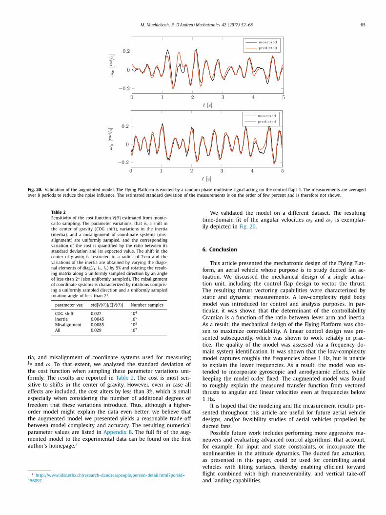
Fig. 20. Validation of the augmented model. The Flying Platform is excited by a random phase multisine signal acting on the control flaps 1. The measurements are averaged

over 8 periods to reduce the noise influence. The estimated standard deviation of the measurements is on the order of few percent and is therefore not shown.

Table 2

Sensitivity of the cost function V ( θ ) estimated from monte-

carlo sampling. The parameter variations, that is, a shift in

the center of gravity (COG shift), variations in the inertia

(inertia), and a misalignment of coordinate systems (mis-

alignment) are uniformly sampled, and the corresponding

variation of the cost is quantified by the ratio between its

standard deviation and its expected value. The shift in the

center of gravity is restricted to a radius of 2 cm and the

variations of the inertia are obtained by varying the diago-

nal elements of diag( I 1 , I 1 , I 3 ) by 5% and rotating the result-

ing matrix along a uniformly sampled direction by an angle

of less than 2 ° (also uniformly sampled). The misalignment

of coordinate systems is characterized by rotations compris-

ing a uniformly sampled direction and a uniformly sampled

rotation angle of less than 2 °.

parameter var. std[ V ( θ )]/E[ V ( θ )] Number samples

COG shift 0 .027 10 4

Inertia 0 .0045 10 5

Misalignment 0 .0085 10 5

All 0 .029 10 7

t

J

t

f

s

e

e

f

o

t

b

p

m

a

1

t

i

6

f

t

t

T

s

m

t

G

A

s

s

t

m

m

t

t

k

t

t

1

s

d

d

n

f

ia, and misalignment of coordinate systems used for measuring v and ω. To that extent, we analyzed the standard deviation of

he cost function when sampling these parameter variations uni-

ormly. The results are reported in Table 2 . The cost is most sen-

itive to shifts in the center of gravity. However, even in case all

ffects are included, the cost alters by less than 3%, which is small

specially when considering the number of additional degrees of

reedom that these variations introduce. Thus, although a higher-

rder model might explain the data even better, we believe that

he augmented model we presented yields a reasonable trade-off

etween model complexity and accuracy. The resulting numerical

arameter values are listed in Appendix B . The full fit of the aug-

ented model to the experimental data can be found on the first

uthor’s homepage. 7

7 http://www.idsc.ethz.ch/research-dandrea/people/person-detail.html?persid=

56097 .

n

a

v

fl

a

We validated the model on a different dataset. The resulting

ime-domain fit of the angular velocities ω x and ω y is exemplar-

ly depicted in Fig. 20 .

. Conclusion

This article presented the mechatronic design of the Flying Plat-

orm, an aerial vehicle whose purpose is to study ducted fan ac-

uation. We discussed the mechanical design of a single actua-

ion unit, including the control flap design to vector the thrust.

he resulting thrust vectoring capabilities were characterized by

tatic and dynamic measurements. A low-complexity rigid body

odel was introduced for control and analysis purposes. In par-

icular, it was shown that the determinant of the controllability

ramian is a function of the ratio between lever arm and inertia.

s a result, the mechanical design of the Flying Platform was cho-

en to maximize controllability. A linear control design was pre-

ented subsequently, which was shown to work reliably in prac-

ice. The quality of the model was assessed via a frequency do-

ain system identification. It was shown that the low-complexity

odel captures roughly the frequencies above 1 Hz, but is unable

o explain the lower frequencies. As a result, the model was ex-

ended to incorporate gyroscopic and aerodynamic effects, while

eeping the model order fixed. The augmented model was found

o roughly explain the measured transfer function from vectored

hrusts to angular and linear velocities even at frequencies below

Hz.

It is hoped that the modeling and the measurement results pre-

ented throughout this article are useful for future aerial vehicle

esigns, and/or feasibility studies of aerial vehicles propelled by

ucted fans.

Possible future work includes performing more aggressive ma-

euvers and evaluating advanced control algorithms, that account,

or example, for input and state constraints, or incorporate the

onlinearities in the attitude dynamics. The ducted fan actuation,

s presented in this paper, could be used for controlling aerial

ehicles with lifting surfaces, thereby enabling efficient forward

ight combined with high maneuverability, and vertical take-off

nd landing capabilities.

66 M. Muehlebach, R. D’Andrea / Mechatronics 42 (2017) 52–68

Y

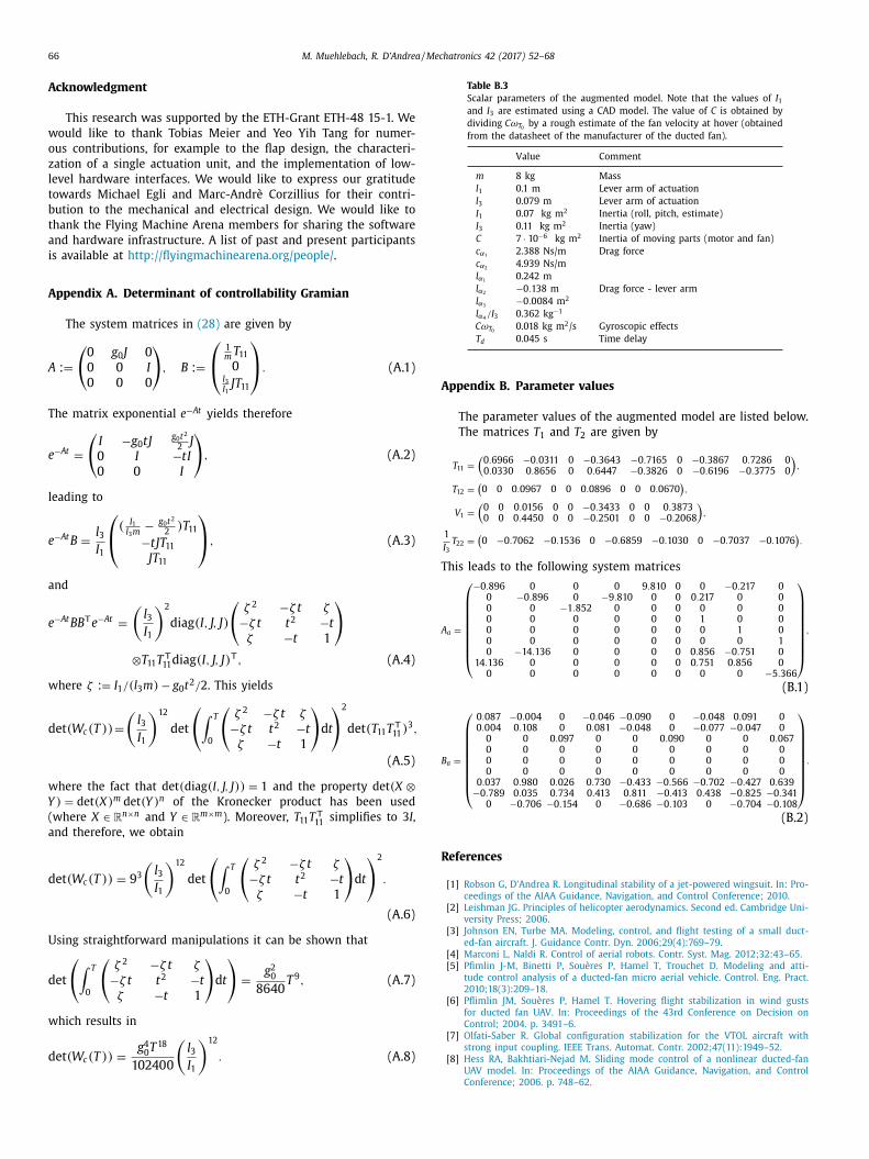
Table B.3

Scalar parameters of the augmented model. Note that the values of I 1 and I 3 are estimated using a CAD model. The value of C is obtained by

dividing Cω T 0 by a rough estimate of the fan velocity at hover (obtained

from the datasheet of the manufacturer of the ducted fan).

Value Comment

m 8 kg Mass

l 1 0.1 m Lever arm of actuation

l 3 0.079 m Lever arm of actuation

I 1 0 .07 kg m

2 Inertia (roll, pitch, estimate)

I 3 0 .11 kg m

2 Inertia (yaw)

C 7 · 10 −6 kg m

2 Inertia of moving parts (motor and fan)

c α1 2.388 Ns/m Drag force

c α2 4.939 Ns/m

l α1 0.242 m

l α2 −0 . 138 m Drag force - lever arm

l α3 −0 . 0084 m

2

l α4 /I 3 0.362 kg −1

Cω T 0 0 .018 kg m

2 /s Gyroscopic effects

T d 0.045 s Time delay

A

T

A

B

R

Acknowledgment

This research was supported by the ETH-Grant ETH-48 15-1. We

would like to thank Tobias Meier and Yeo Yih Tang for numer-

ous contributions, for example to the flap design, the characteri-

zation of a single actuation unit, and the implementation of low-

level hardware interfaces. We would like to express our gratitude

towards Michael Egli and Marc-Andrè Corzillius for their contri-

bution to the mechanical and electrical design. We would like to

thank the Flying Machine Arena members for sharing the software

and hardware infrastructure. A list of past and present participants

is available at http://flyingmachinearena.org/people/ .

Appendix A. Determinant of controllability Gramian

The system matrices in (28) are given by

A :=

(

0 g 0 J 0

0 0 I 0 0 0

)

, B :=

⎛ ⎝

1 m

T 11

0

l 3 I 1

JT 11

⎞ ⎠ . (A.1)

The matrix exponential e −At yields therefore

e −At =

(

I −g 0 tJ g 0 t 2

2 J

0 I −tI 0 0 I

)

, (A.2)

leading to

e −At B =

l 3 I 1

⎛ ⎝

( I 1 l 3 m

− g 0 t 2

2 ) T 11

−tJT 11

JT 11

⎞ ⎠ , (A.3)

and

e −At BB

T e −At =

(l 3 I 1

)2

diag (I, J, J)

(

ζ 2 −ζ t ζ−ζ t t 2 −t ζ −t 1

)

�T 11 T T

11 diag (I, J, J) T , (A.4)

where ζ := I 1 / (l 3 m ) − g 0 t 2 / 2 . This yields

det (W c (T )) =

(l 3 I 1

)12

det

( ∫ T

0

(

ζ 2 −ζ t ζ−ζ t t 2 −t ζ −t 1

)

d t

) 2

det (T 11 T T

11 ) 3 ,

(A.5)

where the fact that det ( diag (I, J, J)) = 1 and the property det (X �

) = det (X ) m det (Y ) n of the Kronecker product has been used

(where X ∈ R

n ×n and Y ∈ R

m ×m ). Moreover, T 11 T T

11 simplifies to 3 I ,

and therefore, we obtain

det (W c (T )) = 9

3

(l 3 I 1

)12

det

( ∫ T

0

(

ζ 2 −ζ t ζ−ζ t t 2 −t ζ −t 1

)

d t

) 2

.

(A.6)

Using straightforward manipulations it can be shown that

det

( ∫ T

0

(

ζ 2 −ζ t ζ−ζ t t 2 −t ζ −t 1

)

d t

)

=

g 2 0

8640

T 9 , (A.7)

which results in

det (W c (T )) =

g 4 0 T 18

102400

(l 3 I 1

)12

. (A.8)

ppendix B. Parameter values

The parameter values of the augmented model are listed below.

The matrices T 1 and T 2 are given by

T 11 =

(0 . 6966 −0 . 0311 0 −0 . 3643 −0 . 7165 0 −0 . 3867 0 . 7286 0 0 . 0330 0 . 8656 0 0 . 6447 −0 . 3826 0 −0 . 6196 −0 . 3775 0

),

T 12 =

(0 0 0 . 0967 0 0 0 . 0896 0 0 0 . 0670

),

V 1 =

(0 0 0 . 0156 0 0 −0 . 3433 0 0 0 . 3873 0 0 0 . 4450 0 0 −0 . 2501 0 0 −0 . 2068

),

1

I 3 T 22 =

(0 −0 . 7062 −0 . 1536 0 −0 . 6859 −0 . 1030 0 −0 . 7037 −0 . 1076

).

his leads to the following system matrices

a =

⎛ ⎜ ⎜ ⎜ ⎜ ⎜ ⎜ ⎜ ⎜ ⎝

−0 . 896 0 0 0 9 . 810 0 0 −0 . 217 0 0 −0 . 896 0 −9 . 810 0 0 0 . 217 0 0 0 0 −1 . 852 0 0 0 0 0 0 0 0 0 0 0 0 1 0 0 0 0 0 0 0 0 0 1 0 0 0 0 0 0 0 0 0 1 0 −14 . 136 0 0 0 0 0 . 856 −0 . 751 0

14 . 136 0 0 0 0 0 0 . 751 0 . 856 0 0 0 0 0 0 0 0 0 −5 . 366

⎞ ⎟ ⎟ ⎟ ⎟ ⎟ ⎟ ⎟ ⎟ ⎠

,

(B.1)

a =

⎛ ⎜ ⎜ ⎜ ⎜ ⎜ ⎜ ⎜ ⎜ ⎝

0 . 087 −0 . 004 0 −0 . 046 −0 . 090 0 −0 . 048 0 . 091 0 0 . 004 0 . 108 0 0 . 081 −0 . 048 0 −0 . 077 −0 . 047 0

0 0 0 . 097 0 0 0 . 090 0 0 0 . 067 0 0 0 0 0 0 0 0 0 0 0 0 0 0 0 0 0 0 0 0 0 0 0 0 0 0 0

0 . 037 0 . 980 0 . 026 0 . 730 −0 . 433 −0 . 566 −0 . 702 −0 . 427 0 . 639 −0 . 789 0 . 035 0 . 734 0 . 413 0 . 811 −0 . 413 0 . 438 −0 . 825 −0 . 341

0 −0 . 706 −0 . 154 0 −0 . 686 −0 . 103 0 −0 . 704 −0 . 108

⎞ ⎟ ⎟ ⎟ ⎟ ⎟ ⎟ ⎟ ⎟ ⎠

.

(B.2)

eferences

[1] Robson G , D’Andrea R . Longitudinal stability of a jet-powered wingsuit. In: Pro-

ceedings of the AIAA Guidance, Navigation, and Control Conference; 2010 . [2] Leishman JG . Principles of helicopter aerodynamics. Second ed. Cambridge Uni-

versity Press; 2006 .

[3] Johnson EN , Turbe MA . Modeling, control, and flight testing of a small duct-ed-fan aircraft. J. Guidance Contr. Dyn. 2006;29(4):769–79 .

[4] Marconi L , Naldi R . Control of aerial robots. Contr. Syst. Mag. 2012;32:43–65 . [5] Pfimlin J-M , Binetti P , Souères P , Hamel T , Trouchet D . Modeling and atti-

tude control analysis of a ducted-fan micro aerial vehicle. Control. Eng. Pract.2010;18(3):209–18 .

[6] Pflimlin JM , Souères P , Hamel T . Hovering flight stabilization in wind gustsfor ducted fan UAV. In: Proceedings of the 43rd Conference on Decision on

Control; 2004. p. 3491–6 .

[7] Olfati-Saber R . Global configuration stabilization for the VTOL aircraft withstrong input coupling. IEEE Trans. Automat. Contr. 2002;47(11):1949–52 .

[8] Hess RA , Bakhtiari-Nejad M . Sliding mode control of a nonlinear ducted-fanUAV model. In: Proceedings of the AIAA Guidance, Navigation, and Control

Conference; 2006. p. 748–62 .

M. Muehlebach, R. D’Andrea / Mechatronics 42 (2017) 52–68 67

[

[

[

[

[

[

[

[9] Franz R , Milam M , Hauser J . Applied receding horizon control of the cal-tech ducted fan. In: Proceedings of the American Control Conference; 2002.

p. 3735–40 . [10] Peddle IK , Jones T , Treurnicht J . Practical near hover flight control of a ducted

fan (SLADe). Control Eng. Pract. 2009;17(1):48–58 . [11] Fleming J , Jones T , Ng W , Gelhausen P , Enns D . Improving control system ef-

fectiveness for ducted fan VTOL UAVs operating in crosswinds. In: Proceed-ings of the 2nd AIAA “Unmanned Unlimited” System, Technologies and Opera-

tions-Aerospace Conference; 2003 .

[12] Pereira JL . Hover and Wind-Tunnel Testing of Shrouded Rotors for ImprovedMicro Air Vehicle Design. Ph.D. thesis. University of Maryland; 2008 .

[13] Akturk A , Camci C . Experimental and computational assessment of a ducted–fan rotor flow model. J. Aircr. 2012;49(3):885–97 .

[14] Hrishikeshavan V , Black J , Chopra I . Development of a quad shrouded rotormircro air vehicle and performance evaluation in edgewise flow. In: Proceed-

ings of the American Helicopter Society Forum; 2012 .

[15] Miwa M , Uemura S , Ishihara Y , Imamura A , hwan Shim J , Ioi K . Evaluation ofquad ducted-fan helicopter. Int. J. Intell. Unmanned Syst. 2013;1(2):187–98 .

[16] Imamura A , Miwa M , Hino J . Flight characteristics of quad rotor helicopter withthrust vectoring equipment. J. Rob. Mech. 2016;28(3):334–42 .

[17] Hamel PG , Jategaonkar RV . Evolution of flight vehicle system identification. J.Aircr. 1996;33(1):9–28 .

[18] Mettler B , Tischler MB , Kanade T . System identification of small-size un-

manned helicopter dynamics. In: Proceedings of the American Helicopter So-ciety Forum; 1999 .

[19] Dorobantu A , Murch AM , Mettler B , Balas GJ . Frequency domain system iden-tification for a small, low-cost, fixed-wing UAV. In: Proceedings of the AIAA

Guidance, Navigation, and Control Conference; 2011 . 20] Derafa L , Madani T , Benallegue A . Dynamic modelling and experimental iden-

tification of four rotors helicopter parameters. In: Proceedings of the Interna-tional Conference on Industrial Technology; 2006. p. 1834–9 .

[21] Hoffer NV , Coopmans C , Jensen AM , Chen Y . A survey and categorization ofsmall low-cost unmanned aerial vehicle system identification. J. Intell. Rob.

Syst. 2014;74(1):129–45 .

22] Lewis KW . The Cumulative Effects of Roughness and Reynolds Number onNACA 0015 Airfoil Section Characteristics. Texas Tech University; 1984. Mas-

ter’s thesis in Mechanical Engineering . 23] Freudenreich K , Kaiser K , Schaffarczyk A , Winkler H , Stahl B . Reynolds num-

ber and roughness effects on thick airfoils for wind turbines. Wind Eng.2004;28(5):529–46 .

24] PX4 flight management unit. https://pixhawk.org/modules/px4fmu ; Accessed:

July 2016. 25] Pfeiffer F , Glocker C . Multibody Dynamics with Unilateral Contacts. Wiley-VCH;

2004 . 26] Callier FM , Desoer CA . Linear System Theory. Springer Science + Business Me-

dia; 1991 . [27] Lupashin S , Hehn M , Mueller MW , Schoellig AP , Sherback M , D’Andrea R . A

platform for aerial robotics research and demonstration: the flying machine

arena. Mechatronics 2014;24:41–54 . 28] Pintelon R , Schoukens J . System Identification: A Frequency Domain Approach.

Second ed. John Wiley & Sons; 2012 .

68 M. Muehlebach, R. D’Andrea / Mechatronics 42 (2017) 52–68

0 and 2013, respectively. He received the Outstanding D-MAVT Bachelor Award and was nd Control. He did his Master’s thesis on variational integrators for Hamiltonian systems

H Zurich in the Institute for Dynamic Systems and Control. His main interests include l.

ersity of Toronto in 1991, and the M.S. and Ph.D. degrees in Electrical Engineering from

en an associate, professor at Cornell University from 1997 to 2007. While on leave from

C s architecture, robot design, robot navigation and coordination, and control algorithms

d chairman of the board at Verity Studios AG.

Michael Muehlebach received the B.Sc. and M.Sc. degrees from ETH Zurich in 201awarded the Willi-Studer prize for the best Master’s degree in Robotics, Systems, a

and their application to multibody dynamics. He is currently a PhD student at ETmultibody dynamics, the control of nonlinear systems, and model predictive contro

Raffaello D’Andrea received the B.Sc. degree in Engineering Science from the Univ

the California Institute of Technology in 1992 and 1997. He was an assistant, and thornell, from 2003 to 2007, he co-founded Kiva Systems, where he led the system

effort s. He is currently professor of Dynamic Systems and Control at ETH Zurich, an