The flow fields involved in hydrodynamic imaging by blind Mexican

3819

INTRODUCTIONFish have the potential to be able to sense their surroundings bysensing changes in the flow fields generated around their bodies asthey swim through the water. Fish are able to get information aboutnearby objects by sensing the changes the presence of objects causein the flow field; this is known as hydrodynamic imaging (Hassan,1989). This is best known to be used by the hypogean (cave-dwelling) form of Astyanax fasciatus Cuvier 1819, commonlyknown as the blind Mexican cave fish (von Campenhausen et al.,1981; Weissert and von Campenhausen, 1981).

Fish are able to sense water motion using their lateral linemechanosensory system. The lateral line is composed of individualsensory organs called neuromasts. Each neuromast is composed ofa group of hair cells that project their sensory cilia into a gelatinouscupula. When the cupula is displaced by motion of the surroundingfluid the hair cells are stimulated, sending information to the centralnervous system. There are two sub-systems of neuromasts, whichmake up the lateral line. Superficial neuromasts are located on thesurface of the skin and their cupula are displaced in proportion tothe velocity of the flow, encoding the velocity component of theflow field (Kalmijn, 1988). Canal neuromasts sit in canals underthe surface of the skin and are located between pores that open tothe surrounding water. The cupula of canal neuromasts are displacedin proportion to the difference in pressure between the pores to eitherside, encoding the gradient of the pressure component of the flowfield (Denton and Gray, 1983; Denton and Gray, 1988). For a fullreview of the lateral line system, see Coombs and Montgomery(Coombs and Montgomery, 1999).

In order to understand how fish use flow-field distortions to sensetheir surroundings it is necessary to understand the nature of theflow field around the fish and how the flow field is altered by the

presence of objects. It is then possible to estimate how these changesmay be encoded by the lateral line. Blind cave fish are the mostrecognised species of fish that are known to use hydrodynamicimaging, but it is highly likely that other fish species also have thisability. Numerous studies using experimentally blinded fish of otherspecies have observed blinded fish avoiding obstacles withouttouching them (Dijkgraaf, 1963; Partridge and Pitcher, 1980; Teyke,1988; Yasuda, 1973), presumably by using hydrodynamic imaging.Hydrodynamic imaging appears to be most effective when fish aregliding with their body held straight; blind cave fish spendapproximately 70% of their time gliding (Windsor et al., 2008).Hence it is the flow field around fish when gliding that is of mostinterest when studying hydrodynamic imaging.

There is a considerable amount known about the flow fieldsinvolved with the propulsion of fish (for a review, see Drucker andLauder, 2002), but surprisingly little about the flow fields aroundgliding fish. Dubois et al. fitted live bluefish (Pomatomus saltatrix)with Pitot pressure tubes and measured the pressure fields on thebody surface of the fish as they swam (Dubois et al., 1974). Astagnation point was found at the jaw of the fish, with positivepressure at the front of the fish, becoming negative as the width ofthe body increased and then becoming positive again towards thetail. Kuiper also briefly examined the pressure distribution arounda fish-shaped model using a Pitot pressure tap system and found asimilarly shaped pressure variation along the body (Kuiper, 1967).

The stimulus to the lateral line generated by the hydrodynamicinteraction of a three-dimensional (3-D) fish shape and a flat surfacehas been investigated in a series of mathematical modelling studiesby Hassan (Hassan, 1985; Hassan, 1992a; Hassan, 1992b). Thesestudies were based on potential flow modelling, which simulatesflows at very high Reynolds numbers (Re). In potential flow models,

The Journal of Experimental Biology 213, 3819-3831© 2010. Published by The Company of Biologists Ltddoi:10.1242/jeb.040741

The flow fields involved in hydrodynamic imaging by blind Mexican cave fish(Astyanax fasciatus). Part I: open water and heading towards a wall

Shane P. Windsor*, Stuart E. Norris, Stuart M. Cameron, Gordon D. Mallinson and John C. MontgomerySchool of Biological Sciences, University of Auckland, Private Bag 92019, Auckland 1142, New Zealand

*Author for correspondence at present address: University of Oxford, Department of Zoology, Tinbergen Building, South Parks Road,Oxford OX1 3PS, UK ([email protected])

Accepted 23 August 2010

SUMMARYBlind Mexican cave fish (Astyanax fasciatus) sense the presence of nearby objects by sensing changes in the water flow aroundtheir body. The information available to the fish using this hydrodynamic imaging ability depends on the properties of the flowfield it generates while gliding and how this flow field is altered by the presence of objects. Here, we used particle imagevelocimetry to measure the flow fields around gliding blind cave fish as they moved through open water and when headingtowards a wall. These measurements, combined with computational fluid dynamics models, were used to estimate the stimulusto the lateral line system of the fish. Our results showed that there was a high-pressure region around the nose of the fish, low-pressure regions corresponding to accelerated flow around the widest part of the body and a thick laminar boundary layer downthe body. When approaching a wall head-on, the changes in the stimulus to the lateral line were confined to approximately thefirst 20% of the body. Assuming that the fish are sensitive to a certain relative change in lateral line stimuli, it was found thatswimming at higher Reynolds numbers slightly decreased the distance at which the fish could detect a wall when approachinghead-on, which is the opposite to what has previously been expected. However, when the effects of environmental noise areconsidered, swimming at higher speed may improve the signal to noise ratio of the stimulus to the lateral line.

Key words: Astyanax fasciatus, biomechanics, blind cave fish, computational fluid dynamics, hydrodynamic imaging, lateral line.

THE JOURNAL OF EXPERIMENTAL BIOLOGY

3820

the fluid is assumed to be inviscid and, as such, viscous boundarylayers are not modelled. This may be a major limitation in thesemodels, as the presence of viscous boundary layers could beexpected to have a large impact on the form of the flow field arounda small fish at low Re and, hence, the effective stimulus to the lateralline.

The objectives of this study were to determine the availablestimulus to the lateral line by measuring the flow fields aroundgliding blind cave fish, and to determine how these flow fields werealtered through interactions with external surfaces. The flow fieldsaround cave fish gliding through open water and gliding head-ontowards a wall were measured experimentally using particle imagevelocimetry (PIV). Measured flow fields were used to validatecomputational fluid dynamic (CFD) models constructed for thesesame situations. These models were then used to estimate the lateralline stimulus. In a companion paper the flow fields around fishgliding parallel to a wall were studied using similar techniques(Windsor et al., 2010). The kinematics and behaviour of blind cavefish in these same situations has previously been measured in detail(Windsor et al., 2008), allowing comparisons to be made betweenthe behaviour of the fish and the sensory information that ispotentially available.

MATERIALS AND METHODSFish

Blind Mexican cave fish were purchased from a commercialaquarium supplier. The fish ranged in size from 40 to 60mm intotal length, with a mean (±s.e.m.) length of 44±4mm. The fishwere housed as described previously (Windsor et al., 2008). Allexperiments were carried out in accordance with the animal carepolicy of the University of Auckland.

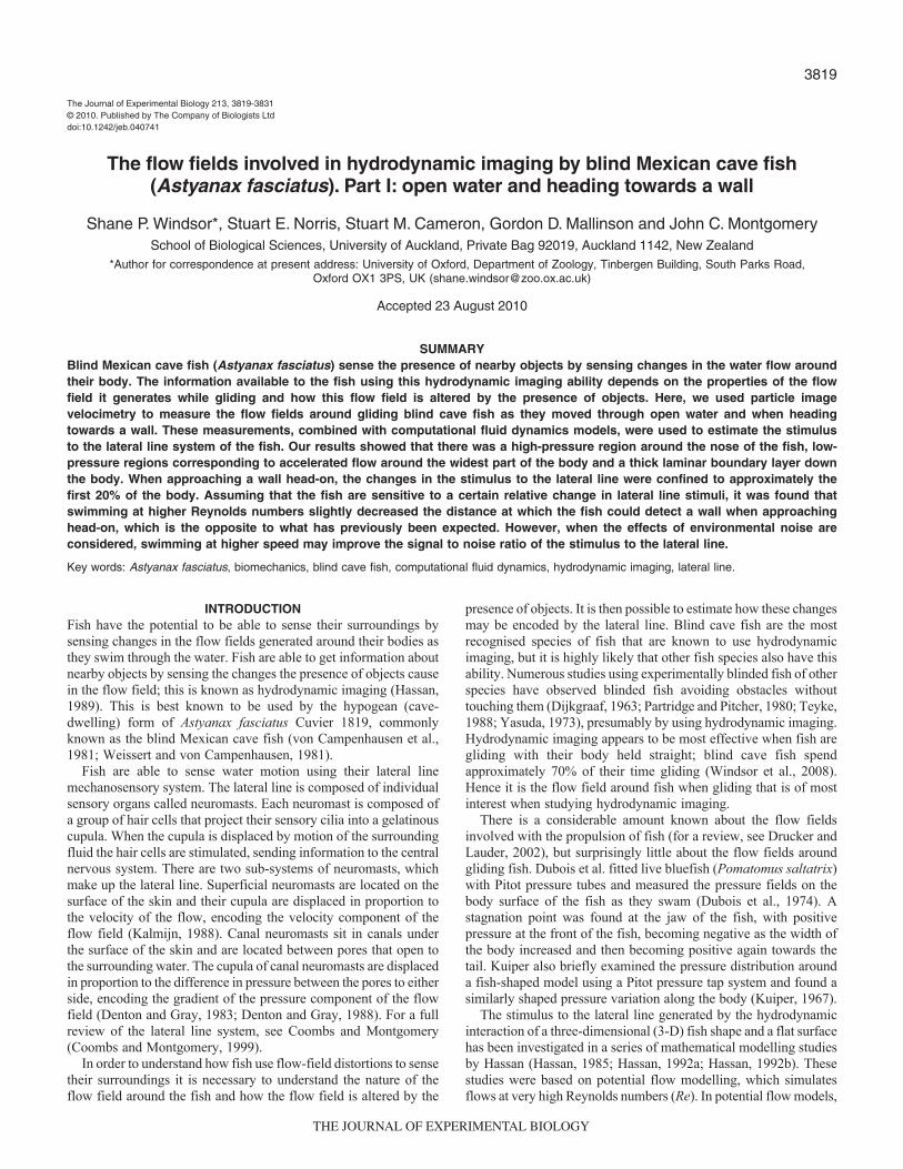
Experimental procedurePIV measurements were made of individual fish swimming freelyin a glass experimental tank measuring 400mm�300mm�80mm(length � breadth � height: Fig.1). The tank had a short partitionmidway down the longer wall to direct the fish to swim across thetank, head-on toward a submerged wall on the opposite side of thetank. The top of this wall was slightly below the surface of the waterin order to prevent optical distortions created by any meniscus at thesurface. The PIV system was set up to look directly down this wall,midway along the tank in a horizontal plane 10mm above the tankbottom for smaller fish (<50mm in length), or 15mm above thebottom for larger fish (>50mm in length). The field of view of thePIV camera was 23mm�23mm. Two additional cameras (MarlinF131B, AVT, Stadtroda, Germany) were also used to record the fish’sbehaviour before and after it passed through the field of view of thePIV camera and to record the height at which the fish swam throughthe laser sheet. The length of the trials was limited to 9min by thecapacity of the computer hard disk drive array recording the PIVimages. The water in the experimental tank was completely still apartfrom the motion generated by the movement of the fish. Betweentrials an aerator and heater were placed in the experimental tank tomaintain the temperature (25°C) and oxygen level of the water.

The particle image velocimetry systemPIV measurements were made using a custom built PIV system(Schlicke et al., 2007). The system used an oscillating mirror drivenby a galvanometer in combination with a continuous laser (5W532nm Nd:YVO4 laser, Spectra-Physics Millenia, Santa Clara, CA,USA) to generate a laser light sheet approximately 1mm thick. ThePIV camera (Basler A504k, Ahrensburg, Germany) captured 8bit

monochrome 960�960 pixel images at 200framess–1. The waterwas seeded with neutrally buoyant 10m diameter hollow glassspheres.

Particle image velocimetry processingEach PIV video sequence was reviewed before processing and onlypasses where a fish was gliding in still water, in a straight line, withno noticeable pitch or roll relative to the laser plane were analysed.In addition, only passes where the laser sheet visibly intersected afish mid way up the dorsal–ventral axis without reflection wereconsidered, in order to minimise any out of plane flows. Full 3-DCFD modelling studies of swimming giant danio (Daniomalabaricus) have shown that the flow field is strongly two-dimensional (2-D) along the mid body plane of this similarly shapedfish (Wolfgang et al., 1999).

A series of image processing procedures was performed usingcustom written software (Cameron, 2007) before calculating thevelocity vector field. Any glare around the fish was removed bysubtracting a median filtered copy of the image. The edge of thefish intersecting the laser sheet was then detected using an intensity-gradient-based Canny edge detector and the body of the fish wasmasked out by mirroring this edge about the mid-line of the fish.

The flow velocity field was calculated from the processed imagesusing an iterative cross-correlation algorithm with a finalinterrogation window of 32�32 pixels with a 50% window overlap,giving a 60�60 field of velocity vectors. The cross-correlationalgorithm utilised a continuous-window shift with a linear velocitygradient correction to compensate for the steep velocity gradientsin the boundary layer around the fish. The total estimated error ofthe PIV system and the cross-correlation methods used wasapproximately ±1% (Cameron, 2007). Velocity vectors were notcalculated for any interrogation regions that overlapped the bodyof the fish in order to avoid erroneous vectors. The velocity of afish was calculated by cross-correlating images of its outline.

The interpretation of the velocity field was also aided by makingartificial particle streak images from the PIV video sequences. Thiswas done by thresholding each PIV image to create a binary imageand then segmenting out the body of the fish. This left only the

S. P. Windsor and others

Top camera

PIV cameraPIV camera field of view

Top camera field of view

Submergedwall

Partition

SIDE VIEW TOP VIEWP

Side camera

Side camera field of view

er light Laseheetsh

Fig.1. Diagram of experimental setup for particle image velocimetry (PIV)measurements (not to scale). A partition in the middle of the tank directedthe fish to approach the submerged wall on the opposite side of the tank.The PIV camera recorded the motion of particles in the laser light sheet,and the movements of the fish were recorded from above and from theside by two additional cameras.


3821Hydrodynamic imaging in open water

brightest particles in the image. Series of consecutive frames werethen added together to form particle streak images, which showedthe structure of the velocity field. The particle streak images wereparticularly effective in visualising the boundary layer flow closeto the fish, whereas the PIV velocity vectors did not have sufficientresolution to do so.

Pressure field calculationAs the lateral line is capable of sensing both the velocity and pressuregradient of the surrounding fluid flow, it was desirable to measureboth the velocity and pressure components of the flows around thefish. PIV is traditionally only used to measure the velocity field,but it is also possible to estimate the pressure field from the velocityfield using the Poisson pressure relationship (Fujisawa et al., 2004;Fujisawa et al., 2006; Fujisawa et al., 2005; Gurka et al., 1999;Hosokawa et al., 2003; Murai et al., 2007). A finite differenceapproach was used, with the pressure gradient field being calculatedfrom experimental velocity data using the Navier–Stokes equations.This was then related to the pressure distribution using a pressurePoisson equation [see Windsor (Windsor, 2008) for a fulldescription]. In this process it was assumed that at any particularinstant the velocity field was quasi-steady, i.e. the fish was notaccelerating or decelerating significantly. All PIV measurementswere made as the fish decelerated smoothly while gliding. Basedon previous kinematic measurements (Windsor et al., 2008) the meanchange in fish velocity between video frames would have only beenapproximately –0.40% of the swimming velocity of the fish. It wasalso assumed that the flow was laminar with no out of plane flow(divergence free in a 2-D sense). All the flows observed in the PIVexperiments were laminar with no indications of turbulence.

Stimulus estimationThe stimulus to the superficial neuromasts is generally consideredto be the velocity of the flow past each neuromast (Kroese andSchellart, 1992). However, this is complicated by the fact that thecupula is buried within the boundary layer flow on the surface ofthe fish, and in this region the velocity of the flow changes rapidlywith distance from the surface (Jielof et al., 1952; Kalmijn, 1988;Kalmijn, 1989). A superficial neuromast has a cupula that is100–180m long (Teyke, 1990), and responds in proportion to thefluid forces acting on the cupula as a whole (McHenry et al., 2008).As such there is no obvious distance above the skin surface at whichto measure the velocity of the flow. A good approximation of themagnitude of the stimulus to the superficial neuromasts is the wallshear stress (w) (Rapo et al., 2009; Windsor and McHenry, 2009)on the surface of the fish:

where ut is the tangential velocity, y is the direction normal to thesurface and is the dynamic viscosity of the fluid. The wall shearstress is proportional to the difference in velocity between the surfaceof the fish and the fluid surrounding the neuromast. In regions closeto the body where the flow velocity is high, the wall shear stresswill be high, and in regions where the velocity is low, the wall shearstress will be low. The normalised version of the shear stress is theskin friction coefficient (Cf) given by:

where is the density of the fluid and U is swimming speed of thefish, or in the reference frame of the fish, the speed of the oncoming

τw = μ�ut

�y

⎛⎝⎜

⎞⎠⎟

, (1)y=0�

Cf =

τw

0.5 ρU 2, (2)

uniform flow. The superficial neuromasts are distributed in highdensities all over the body of blind cave fish, so the superficialneuromasts were assumed to encode the shear stress at every pointon the body of the fish.

The stimulus to the canal neuromasts is the difference in pressurebetween adjacent canal pores (Denton and Gray, 1983; Kalmijn,1988). The canal pores were assumed to be spaced at 2% body length(BL) intervals based on morphological drawings of blind cave fish(Schemmel, 1967). The stimulus to the first neuromast between thepores 0.02 and 0.04 BL down the fish is plotted as the stimulus at0.02BL. The position of the stimuli on the body was measuredagainst the distance along the surface of the fish from the nose.

To aid in the comparison of flow fields at different Re, the pressure(P) and velocity (u) fields were normalised. The velocity field wasnormalised with respect to the velocity of the fish:

The coefficient of pressure (CP) was used to represent thenormalised pressure field:

The stimulus to the neuromasts of the lateral line system wasestimated based on the same flow field variables for both the PIVmeasurements and the CFD models.

Particle image velocimetry limitationsThe PIV measurements of the flow field around the fish had anumber of limitations. It was difficult to measure the velocity fieldvery close to the body of the fish, as interrogation regions thatoverlapped the body, had to be treated as part of the fish; otherwiseerroneous velocity vectors were calculated. This, coupled with thecomparatively large spacing of the velocity vectors (0.38mm)relative to the thickness of the boundary layer meant that it was notpossible to extract the shear stress distribution on the surface of thefish. The accurate estimation of the pressure field at the edge of thefish was also limited by the resolution of the velocity vectors closeto the body of the fish and by the boundary conditions that had tobe applied in the numerical algorithm for solving the Poissonequation for pressure. The influence of the numerical approximationsto these boundary conditions were extensively tested (Windsor,2008), and when combined with experimental measurement noisewere estimated to introduce a mean (±s.d.) error of approximately6±2% to the calculated pressure values at the boundary of the fish.

Overall, the PIV measurements gave a good representation ofthe general form of the flow field away from the body surface ofthe fish. At the surface of the fish, where we were interested in thestimulus to the lateral line, the PIV measurements were limited bythe spatial resolution of the velocity vectors. For this reason, theexperimental PIV measurements were used to validate the resultsof CFD models in regions of the flow away from the body, and theCFD models were then used to simulate the flows at the surface ofthe fish and to estimate the stimuli to the lateral line.

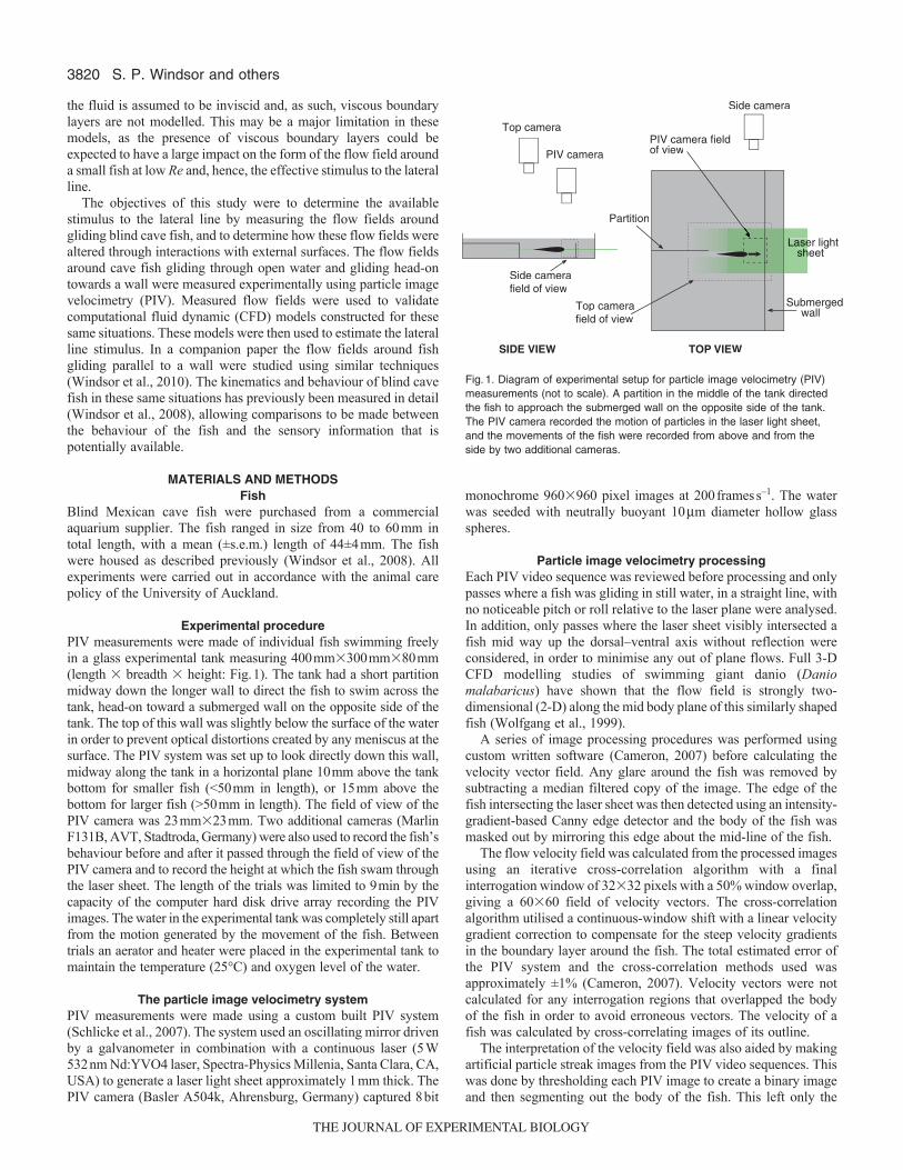
Open water computational fluid dynamic modellingTwo 2-D CFD models and a 3-D model were used to model a fishgliding through open water (Fig.2). The first 2-D model was basedon a NACA 0013 aerofoil, which has the same length to maximumwidth ratio as a blind cave fish. The second 2-D model was a ‘fishshaped’ model representing the cross-sectional shape of the blindcave fish, as seen when looking down at the dorsal surface of the

Unorm =

u

U. (3)

� �

CP =P

0.5 ρU 2. (4)


3822

fish. The shape of the fish was traced from video frames of glidingblind cave fish. For the 3-D modelling, an axisymmetric body ofrevolution based on a NACA 0013 aerofoil, was used to representthe shape of the fish. This shape matched the medial–lateral cross-sectional shape of the fish well (excluding the tail), but did not havethe increased dorsal–ventral height seen in blind cave fish. Thisshape represented the other extreme of geometry from a two-dimensional aerofoil. The true fish shape, with its flattened lateralsurfaces, lies somewhere between the torpedo shaped body ofrevolution and the infinite wing being modelled in the 2-D cases.The 3-D model showed the effects of flow in the dorsal–ventraldirection, although these effects will have been exaggeratedcompared with the true shape of the fish. The models were run atRe ranging from 1000 to 8000, representing the Re range observedin previous behavioural trials (Windsor et al., 2008). Thiscorresponded to swimming velocities ranging from 23 to 180mms–1

for a fish of the mean length used in the PIV trials. The Re wasdefined based on the body length of the fish (L):

In the 2-D models (Fig.3), the boundaries of the square flow domainwere placed 5BL away from the centre of the fish, giving a domainsize of 10�10BL (X�Y), with 64 nodes along each boundary face.A mesh was created around the fish with 256 nodes along each surface,with nodes bunched around the leading and trailing edges of the body,to give a higher mesh resolution in these areas. The mesh had 20structured inflation layers around the fish, so as to accurately capturethe boundary layer flow. The rest of the domain was filled by anunstructured Voronoi mesh. For the 3-D open water model a similargeometry was used, with the domain being 10BL in the Z dimensionand with 20 nodes along each boundary face. A mesh was createdaround the fish with 128 nodes along the length of the fish and 10structured inflation layers around the fish.

All modelling was done using the CFD code (Norris et al., 2010;Were, 1997). The incompressible Navier–Stokes equations weresolved on an unstructured mesh using a scheme that was formallythird order in space and first order in time. See the Appendix forfull details of the CFD methodology used. The flow was assumedto be laminar given the low Re being modelled.

Re =

ULρμ

. (5)

Mesh refinement studies were conducted to establish the meshresolution needed to accurately capture the nature of the flow fieldand quantify the discretisation error. For the 2-D modelling, a NACA0008 aerofoil at a Re of 6000 was used as a test case, for the 3-Dmodelling the axisymmetric body of revolution based on a NACA0013 aerofoil was used. In both cases a range of mesh resolutionswere tested and the results on each mesh compared using Richardsonextrapolation (Roache, 1997). See Appendix for full details and results.


A

C

B

Fig.2. Diagram of the body shapes used in the computational fluiddynamics (CFD) models. (A)2-D NACA 0013 aerofoil. (B)2-D fish shape.(C)3-D axisymmetric body of revolution based on a NACA 0013 aerofoil.

U

X

Y

10 BL

P=0dux/dx=0

Fig.3. Diagram of the 2-D CFD mesh and boundary conditions (not toscale). The body of the fish was in the centre of the domain, with the noseof the fish at the origin and the body aligned with the X-axis. The –X faceof the domain was an inlet, with a uniform inlet velocity based on theReynolds number (Re). The +X face of the domain was set as an outlet,with the pressure set to zero and a zero velocity gradient normal to theboundary. The +Y and –Y faces were set as symmetry planes. The fishgeometry was set as a no slip wall. A very coarse representative mesh isshown. The mesh had structured inflation layers around the fish, while therest of the domain was filled with an unstructured Voronoi mesh.

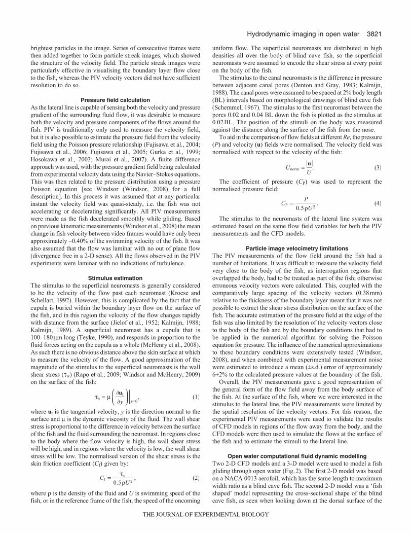
Fig.4. Contour plots of the normalised absolute velocity fields (Unorm) inopen water at a Re of 6000. (A)PIV velocity field, with the wall of the tankat the top of the frame. The shadow of the fish obscures the flow field onthe far side of the fish. Fish body length is 49mm. (B)2-D NACA 0013CFD velocity field. (C)2-D fish-shaped CFD velocity field. (D)3-D NACA0013 body CFD velocity field. The CFD plots are shown in the sameorientation as the PIV data to facilitate comparison.



Head-on computational fluid dynamic modellingTo model the head-on approach of a body towards a wall requiredthe geometry of the model to change as the body moved towardsthe wall. This was implemented in the ALE CFD software using asmoothly deforming unstructured Voronoi mesh, where the boundarynodes of the mesh moved through a defined motion over time. Withinthe mesh, the internal nodes were moved using an iterative smoothingalgorithm, and the connectivity of the nodes recalculated at each stepto maintain a valid Voronoi mesh. The Navier–Stokes equations werecast in the arbitrary Lagrangian Eulerian (ALE) form (Hirt et al.,1974) to enable the flow to be solved on a moving mesh. See Norriset al. for the full details of the ALE method used (Norris et al., 2010).

The same two 2-D shapes as in the open water model were usedto represent the body of a fish: a NACA 0013 aerofoil and a fishshaped geometry. The flow domain was a square, 10�10BL (X�Y)in size, with the –X face of the domain representing a solid wall.The solution process was started with the body aligned along theX-axis, 6BL away from the –X boundary. The body was then movedsteadily towards the wall as the solution progressed, up to the pointwhere the nose of the body was so close to the wall that the formationof a valid mesh was no longer possible. All of the boundaries ofthe domain were set as no slip walls. The fish body was set as a noslip wall with a prescribed velocity of 1BL per unit time.

There were 256 nodes along each side of the fish body, withnodes bunched around the leading and trailing edges of the bodyto give a higher mesh resolution in these areas. There were 10structured inflation layers around the body so as to accurately capturethe boundary layer flow. The body approached the –X boundarywall, which had 736 nodes, with the nodes being bunched aroundthe point where the nose of the body would hit the wall. The +Yand –Y boundaries each had 56 nodes, bunched towards the –X face,and the +X boundary had 32 nodes. The domain was filled with anunstructured Voronoi mesh.

Models were run at Re of 1000, 2000, 4000 and 6000. The meanRe measured for head-on approaches in previous behavioural

experiments was 3000±200 with a range from 960 to 7900 (Windsoret al., 2008). The same time step and body velocity were used inall of the models, with the viscosity of the fluid being varied to alterthe Re. The time step for each iteration was constant and set to keepthe maximum Courant number less than 0.4, in order to maintainthe stability and accuracy of the solution (Anderson, 1995). Theeffect of the size of the time step was quantified (see Appendix forfull details). The flow was assumed to be laminar given the low Rebeing modelled. The pressure at one node, well away from the regionof interest, was set to zero in order to define a reference pressurefor the pressure field.

To verify the implementation of the ALE-based moving mesh,the moving mesh solution was compared with the open water NACA0013 model at a Re of 6000. See Appendix for full details and results.It was found that once the body had moved 4BL then the pressuredistribution was steady and that over the final 2BL as it approachedthe wall, any changes to the flow field were due to the presence ofthe wall.

RESULTSOpen water results

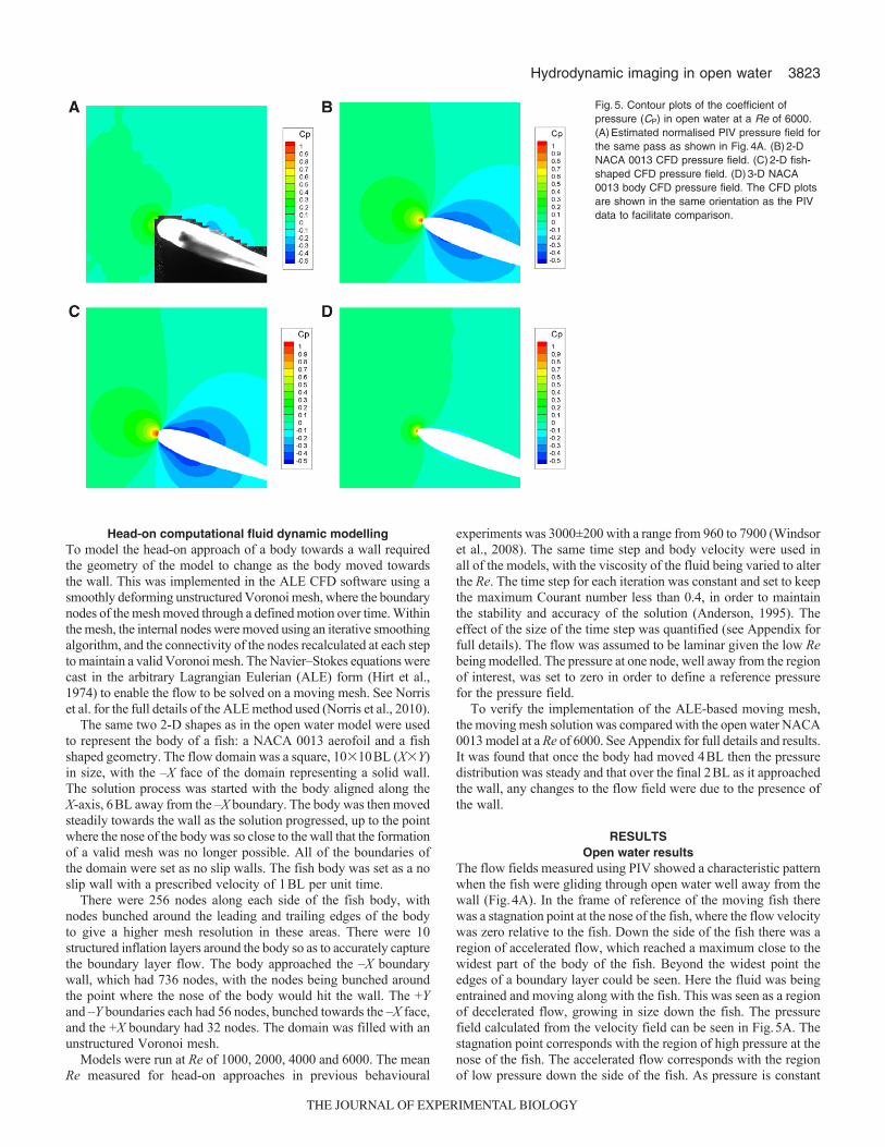
The flow fields measured using PIV showed a characteristic patternwhen the fish were gliding through open water well away from thewall (Fig.4A). In the frame of reference of the moving fish therewas a stagnation point at the nose of the fish, where the flow velocitywas zero relative to the fish. Down the side of the fish there was aregion of accelerated flow, which reached a maximum close to thewidest part of the body of the fish. Beyond the widest point theedges of a boundary layer could be seen. Here the fluid was beingentrained and moving along with the fish. This was seen as a regionof decelerated flow, growing in size down the fish. The pressurefield calculated from the velocity field can be seen in Fig.5A. Thestagnation point corresponds with the region of high pressure at thenose of the fish. The accelerated flow corresponds with the regionof low pressure down the side of the fish. As pressure is constant

Fig.5. Contour plots of the coefficient ofpressure (CP) in open water at a Re of 6000.(A)Estimated normalised PIV pressure field forthe same pass as shown in Fig.4A. (B)2-DNACA 0013 CFD pressure field. (C)2-D fish-shaped CFD pressure field. (D)3-D NACA0013 body CFD pressure field. The CFD plotsare shown in the same orientation as the PIVdata to facilitate comparison.


3824

across a boundary layer (White, 2006) this feature of the flow couldnot be identified in the pressure field. All the flows observed in thePIV experiments were laminar with no indications of turbulence.

The CFD velocity fields around the 2-D NACA 0013 aerofoil andthe 2-D fish shape were very similar to each other (Fig.4B,C). Theyboth showed a large area of reduced velocity in front of the fish andlarge areas of accelerated flow down the sides of the fish. Incomparison, the 3-D aerofoil CFD model (Fig.4D) showed a muchsmaller region of reduced velocity in front of the nose and no part ofthe flow was accelerated above the free stream velocity. The PIVresults indicate that the flow around the fish fell between the 2-D and3-D cases. The CFD models all showed boundary layers of a similarthickness, and the PIV results also suggested the edge of a boundarylayer of a similar thickness. The pressure fields showed similar trendsto the velocity fields (Fig.5B,C,D). Both 2-D CFD models showedlarge high-pressure regions at the nose, as well as large low-pressureregions down the sides of the body. The fish shape had slightly largerhigh- and low-pressure regions than the aerofoil. The 3-D model againshowed much smaller high- and low-pressure regions, reflecting thesmaller accelerations seen in the velocity field. The PIV data againfell between the 2-D and 3-D CFD modelling results.

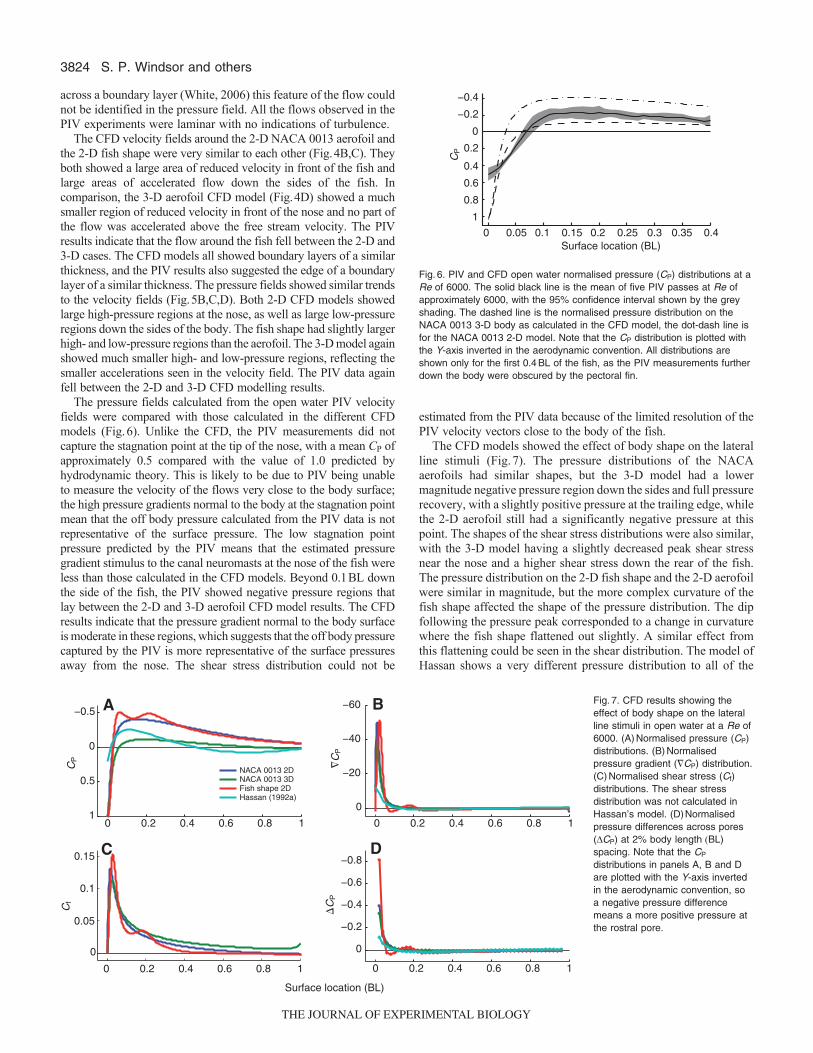
The pressure fields calculated from the open water PIV velocityfields were compared with those calculated in the different CFDmodels (Fig.6). Unlike the CFD, the PIV measurements did notcapture the stagnation point at the tip of the nose, with a mean CP ofapproximately 0.5 compared with the value of 1.0 predicted byhydrodynamic theory. This is likely to be due to PIV being unableto measure the velocity of the flows very close to the body surface;the high pressure gradients normal to the body at the stagnation pointmean that the off body pressure calculated from the PIV data is notrepresentative of the surface pressure. The low stagnation pointpressure predicted by the PIV means that the estimated pressuregradient stimulus to the canal neuromasts at the nose of the fish wereless than those calculated in the CFD models. Beyond 0.1BL downthe side of the fish, the PIV showed negative pressure regions thatlay between the 2-D and 3-D aerofoil CFD model results. The CFDresults indicate that the pressure gradient normal to the body surfaceis moderate in these regions, which suggests that the off body pressurecaptured by the PIV is more representative of the surface pressuresaway from the nose. The shear stress distribution could not be

estimated from the PIV data because of the limited resolution of thePIV velocity vectors close to the body of the fish.

The CFD models showed the effect of body shape on the lateralline stimuli (Fig.7). The pressure distributions of the NACAaerofoils had similar shapes, but the 3-D model had a lowermagnitude negative pressure region down the sides and full pressurerecovery, with a slightly positive pressure at the trailing edge, whilethe 2-D aerofoil still had a significantly negative pressure at thispoint. The shapes of the shear stress distributions were also similar,with the 3-D model having a slightly decreased peak shear stressnear the nose and a higher shear stress down the rear of the fish.The pressure distribution on the 2-D fish shape and the 2-D aerofoilwere similar in magnitude, but the more complex curvature of thefish shape affected the shape of the pressure distribution. The dipfollowing the pressure peak corresponded to a change in curvaturewhere the fish shape flattened out slightly. A similar effect fromthis flattening could be seen in the shear distribution. The model ofHassan shows a very different pressure distribution to all of the


0 0.05 0.1 0.15 0.2 0.25 0.3 0.35 0.4

−0.4

−0.2

0

0.2

0.4

0.6

0.8

1

Surface location (BL)

CP

Fig.6. PIV and CFD open water normalised pressure (CP) distributions at aRe of 6000. The solid black line is the mean of five PIV passes at Re ofapproximately 6000, with the 95% confidence interval shown by the greyshading. The dashed line is the normalised pressure distribution on theNACA 0013 3-D body as calculated in the CFD model, the dot-dash line isfor the NACA 0013 2-D model. Note that the CP distribution is plotted withthe Y-axis inverted in the aerodynamic convention. All distributions areshown only for the first 0.4BL of the fish, as the PIV measurements furtherdown the body were obscured by the pectoral fin.

0 0.2 0.4 0.6 0.8 1

−0.5

0

0.5

10 0.2 0.4 0.6 0.8 1

0 0.2 0.4 0.6 0.8 1


0 0.2 0.4 0.6 0.8 1

−60

−40

−20

0

−0.8

−0.6

−0.4

−0.2

0

NACA 0013 2DNACA 0013 3DFish shape 2DHassan (1992a)

0

0.05

0.1

0.15

A B

DC

�C

P

CP

�C

P

Cf

Fig.7. CFD results showing theeffect of body shape on the lateralline stimuli in open water at a Re of6000. (A)Normalised pressure (CP)distributions. (B)Normalisedpressure gradient (�CP) distribution.(C)Normalised shear stress (Cf)distributions. The shear stressdistribution was not calculated inHassan’s model. (D)Normalisedpressure differences across pores(DCP) at 2% body length (BL)spacing. Note that the CP

distributions in panels A, B and Dare plotted with the Y-axis invertedin the aerodynamic convention, soa negative pressure differencemeans a more positive pressure atthe rostral pore.



CFD models, with positive pressure down the rear half of the fish(Hassan, 1992a). In terms of the normalised pressure differenceacross the canal pores, the maximum stimuli at the nose in Hassan’smodel were only 35% of that predicted by the 3-D CFD model, theclosest comparison in terms of geometry. As Hassan’s model wasinviscid, it was not possible to compare the shear stress distributions.

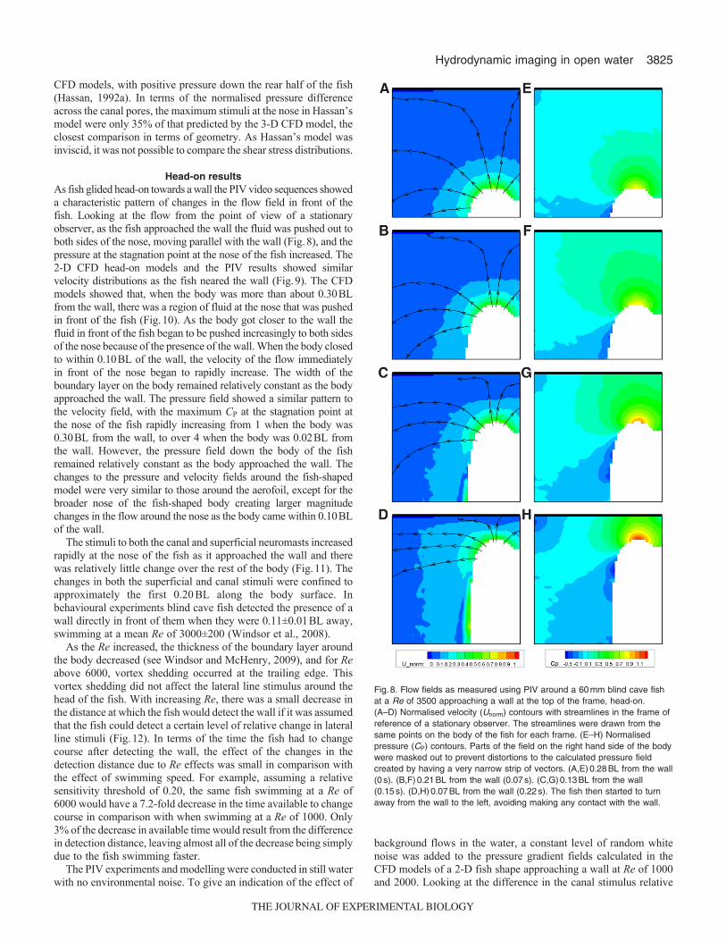
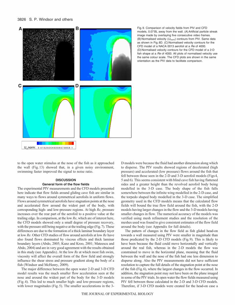
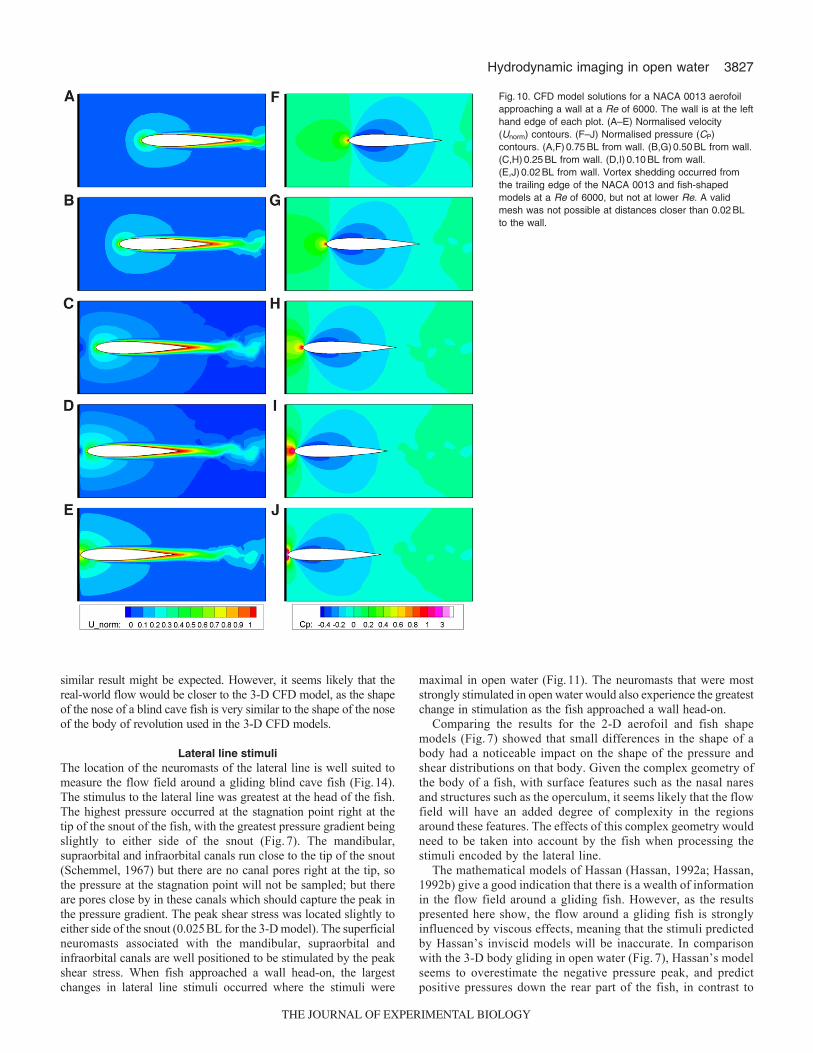
Head-on resultsAs fish glided head-on towards a wall the PIV video sequences showeda characteristic pattern of changes in the flow field in front of thefish. Looking at the flow from the point of view of a stationaryobserver, as the fish approached the wall the fluid was pushed out toboth sides of the nose, moving parallel with the wall (Fig.8), and thepressure at the stagnation point at the nose of the fish increased. The2-D CFD head-on models and the PIV results showed similarvelocity distributions as the fish neared the wall (Fig.9). The CFDmodels showed that, when the body was more than about 0.30BLfrom the wall, there was a region of fluid at the nose that was pushedin front of the fish (Fig.10). As the body got closer to the wall thefluid in front of the fish began to be pushed increasingly to both sidesof the nose because of the presence of the wall. When the body closedto within 0.10BL of the wall, the velocity of the flow immediatelyin front of the nose began to rapidly increase. The width of theboundary layer on the body remained relatively constant as the bodyapproached the wall. The pressure field showed a similar pattern tothe velocity field, with the maximum CP at the stagnation point atthe nose of the fish rapidly increasing from 1 when the body was0.30BL from the wall, to over 4 when the body was 0.02BL fromthe wall. However, the pressure field down the body of the fishremained relatively constant as the body approached the wall. Thechanges to the pressure and velocity fields around the fish-shapedmodel were very similar to those around the aerofoil, except for thebroader nose of the fish-shaped body creating larger magnitudechanges in the flow around the nose as the body came within 0.10BLof the wall.

The stimuli to both the canal and superficial neuromasts increasedrapidly at the nose of the fish as it approached the wall and therewas relatively little change over the rest of the body (Fig.11). Thechanges in both the superficial and canal stimuli were confined toapproximately the first 0.20BL along the body surface. Inbehavioural experiments blind cave fish detected the presence of awall directly in front of them when they were 0.11±0.01BL away,swimming at a mean Re of 3000±200 (Windsor et al., 2008).

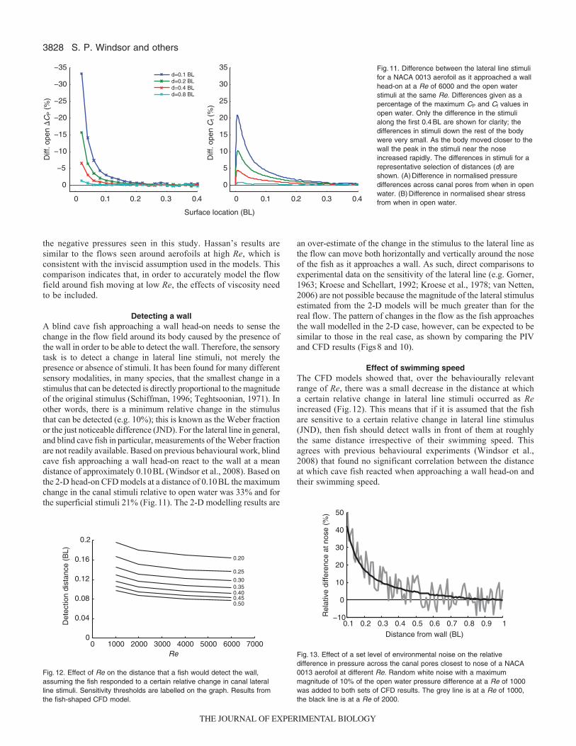
As the Re increased, the thickness of the boundary layer aroundthe body decreased (see Windsor and McHenry, 2009), and for Reabove 6000, vortex shedding occurred at the trailing edge. Thisvortex shedding did not affect the lateral line stimulus around thehead of the fish. With increasing Re, there was a small decrease inthe distance at which the fish would detect the wall if it was assumedthat the fish could detect a certain level of relative change in lateralline stimuli (Fig.12). In terms of the time the fish had to changecourse after detecting the wall, the effect of the changes in thedetection distance due to Re effects was small in comparison withthe effect of swimming speed. For example, assuming a relativesensitivity threshold of 0.20, the same fish swimming at a Re of6000 would have a 7.2-fold decrease in the time available to changecourse in comparison with when swimming at a Re of 1000. Only3% of the decrease in available time would result from the differencein detection distance, leaving almost all of the decrease being simplydue to the fish swimming faster.

The PIV experiments and modelling were conducted in still waterwith no environmental noise. To give an indication of the effect of

background flows in the water, a constant level of random whitenoise was added to the pressure gradient fields calculated in theCFD models of a 2-D fish shape approaching a wall at Re of 1000and 2000. Looking at the difference in the canal stimulus relative

Fig.8. Flow fields as measured using PIV around a 60mm blind cave fishat a Re of 3500 approaching a wall at the top of the frame, head-on.(A–D) Normalised velocity (Unorm) contours with streamlines in the frame ofreference of a stationary observer. The streamlines were drawn from thesame points on the body of the fish for each frame. (E–H) Normalisedpressure (CP) contours. Parts of the field on the right hand side of the bodywere masked out to prevent distortions to the calculated pressure fieldcreated by having a very narrow strip of vectors. (A,E)0.28BL from the wall(0s). (B,F)0.21BL from the wall (0.07s). (C,G)0.13BL from the wall(0.15s). (D,H)0.07BL from the wall (0.22s). The fish then started to turnaway from the wall to the left, avoiding making any contact with the wall.


3826

to the open water stimulus at the nose of the fish as it approachedthe wall (Fig.13) showed that, in a given noisy environment,swimming faster improved the signal to noise ratio.

DISCUSSIONGeneral form of the flow fields

The experimental PIV measurements and the CFD models presentedhere indicate that flow fields around gliding cave fish are similar inmany ways to flows around symmetrical aerofoils in uniform flows.Flows around symmetrical aerofoils have stagnation points at the noseand accelerated flow around the widest part of the body, withcorresponding high- and low-pressure regions. At high Re, pressureincreases over the rear part of the aerofoil to a positive value at thetrailing edge. In comparison, at the low Re, which are of interest here,the CFD models showed only a small degree of pressure recovery,with the pressure still being negative at the trailing edge (Fig.7). Thesedifferences are due to the formation of a thick laminar boundary layerat low Re. Other CFD studies of flow around aerofoils at low Re havealso found flows dominated by viscous effects and thick laminarboundary layers (Abdo, 2005; Kunz and Kroo, 2001; Mateescu andAbdo, 2004) and are in very good agreement with the results obtainedin this study (see Appendix). At the low Re at which most fish swim,viscosity will affect the overall form of the flow field and stronglyinfluence the shear stress and pressure gradient along the body of afish (Windsor and McHenry, 2009).

The major difference between the open water 2-D and 3-D CFDmodel results was the much smaller flow acceleration seen at thenose and around the widest part of the body for the 3-D models(Fig.4). This led to much smaller high- and low-pressure regions,with lower magnitudes (Fig.5). The smaller accelerations in the 3-

D models were because the fluid had another dimension along whichto disperse. The PIV results showed regions of decelerated (highpressure) and accelerated (low pressure) flows around the fish thatfell between those seen in the 2-D and 3-D aerofoil models (Figs4,5 and 6). This seems consistent with blind cave fish having flattenedsides and a greater height than the revolved aerofoil body beingmodelled in the 3-D case. The body shape of the fish fallssomewhere between the infinite wing modelled in the 2-D case, andthe torpedo shaped body modelled in the 3-D case. The simplifiedgeometry used in the CFD models means that the calculated flowfields will bound the true flow field around the fish, with the 2-Dmodels having larger changes in the flow and the 3-D models havingsmaller changes in flow. The numerical accuracy of the models wasverified using mesh refinement studies and the resolution of themeshes used was found to give consistent estimates of the flow fieldaround the body (see Appendix for full details).

The pattern of changes in the flow field as fish glided head-ontowards a wall measured using PIV were smaller in magnitude thanthose predicated by the 2-D CFD models (Fig.9). This is likely tohave been because the fluid could move horizontally and verticallyaround the real fish, whereas in the 2-D models the flow wasconstrained to move in the horizontal plane, meaning that the fluidbetween the wall and the nose of the fish had one less dimension todisperse along. Also the PIV measurements did not have sufficientresolution to capture the full details of the stagnation point at the noseof the fish (Fig.6), where the largest changes in the flow occurred. Inaddition, the stagnation point may not have been on the plane imagedin some of the PIV trials. In open water the flow fields measured usingPIV fell between those calculated in the 2-D and 3-D CFD models.Therefore, if 3-D CFD models were created for the head-on case a


Fig.9. Comparison of velocity fields from PIV and CFDmodels, 0.07BL away from the wall. (A)Artificial particle streakimage made by overlaying five consecutive video frames.(B)Normalised velocity (Unorm) contours from PIV. Same dataas shown in Fig.8D. (C)Normalised velocity contours for theCFD model of a NACA 0013 aerofoil at a Re of 4000.(D)Normalised velocity contours for the CFD model of a 2-Dfish shape at a Re of 4000. All plots of normalised velocity usethe same colour scale. The CFD plots are shown in the sameorientation as the PIV data to facilitate comparison.



similar result might be expected. However, it seems likely that thereal-world flow would be closer to the 3-D CFD model, as the shapeof the nose of a blind cave fish is very similar to the shape of the noseof the body of revolution used in the 3-D CFD models.

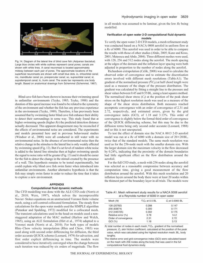
Lateral line stimuliThe location of the neuromasts of the lateral line is well suited tomeasure the flow field around a gliding blind cave fish (Fig.14).The stimulus to the lateral line was greatest at the head of the fish.The highest pressure occurred at the stagnation point right at thetip of the snout of the fish, with the greatest pressure gradient beingslightly to either side of the snout (Fig.7). The mandibular,supraorbital and infraorbital canals run close to the tip of the snout(Schemmel, 1967) but there are no canal pores right at the tip, sothe pressure at the stagnation point will not be sampled; but thereare pores close by in these canals which should capture the peak inthe pressure gradient. The peak shear stress was located slightly toeither side of the snout (0.025BL for the 3-D model). The superficialneuromasts associated with the mandibular, supraorbital andinfraorbital canals are well positioned to be stimulated by the peakshear stress. When fish approached a wall head-on, the largestchanges in lateral line stimuli occurred where the stimuli were

maximal in open water (Fig.11). The neuromasts that were moststrongly stimulated in open water would also experience the greatestchange in stimulation as the fish approached a wall head-on.

Comparing the results for the 2-D aerofoil and fish shapemodels (Fig.7) showed that small differences in the shape of abody had a noticeable impact on the shape of the pressure andshear distributions on that body. Given the complex geometry ofthe body of a fish, with surface features such as the nasal naresand structures such as the operculum, it seems likely that the flowfield will have an added degree of complexity in the regionsaround these features. The effects of this complex geometry wouldneed to be taken into account by the fish when processing thestimuli encoded by the lateral line.

The mathematical models of Hassan (Hassan, 1992a; Hassan,1992b) give a good indication that there is a wealth of informationin the flow field around a gliding fish. However, as the resultspresented here show, the flow around a gliding fish is stronglyinfluenced by viscous effects, meaning that the stimuli predictedby Hassan’s inviscid models will be inaccurate. In comparisonwith the 3-D body gliding in open water (Fig.7), Hassan’s modelseems to overestimate the negative pressure peak, and predictpositive pressures down the rear part of the fish, in contrast to

Fig.10. CFD model solutions for a NACA 0013 aerofoilapproaching a wall at a Re of 6000. The wall is at the lefthand edge of each plot. (A–E) Normalised velocity(Unorm) contours. (F–J) Normalised pressure (CP)contours. (A,F)0.75BL from wall. (B,G)0.50BL from wall.(C,H)0.25BL from wall. (D,I)0.10BL from wall.(E,J)0.02BL from wall. Vortex shedding occurred fromthe trailing edge of the NACA 0013 and fish-shapedmodels at a Re of 6000, but not at lower Re. A validmesh was not possible at distances closer than 0.02BLto the wall.


3828

the negative pressures seen in this study. Hassan’s results aresimilar to the flows seen around aerofoils at high Re, which isconsistent with the inviscid assumption used in the models. Thiscomparison indicates that, in order to accurately model the flowfield around fish moving at low Re, the effects of viscosity needto be included.

Detecting a wallA blind cave fish approaching a wall head-on needs to sense thechange in the flow field around its body caused by the presence ofthe wall in order to be able to detect the wall. Therefore, the sensorytask is to detect a change in lateral line stimuli, not merely thepresence or absence of stimuli. It has been found for many differentsensory modalities, in many species, that the smallest change in astimulus that can be detected is directly proportional to the magnitudeof the original stimulus (Schiffman, 1996; Teghtsoonian, 1971). Inother words, there is a minimum relative change in the stimulusthat can be detected (e.g. 10%); this is known as the Weber fractionor the just noticeable difference (JND). For the lateral line in general,and blind cave fish in particular, measurements of the Weber fractionare not readily available. Based on previous behavioural work, blindcave fish approaching a wall head-on react to the wall at a meandistance of approximately 0.10BL (Windsor et al., 2008). Based onthe 2-D head-on CFD models at a distance of 0.10BL the maximumchange in the canal stimuli relative to open water was 33% and forthe superficial stimuli 21% (Fig.11). The 2-D modelling results are

an over-estimate of the change in the stimulus to the lateral line asthe flow can move both horizontally and vertically around the noseof the fish as it approaches a wall. As such, direct comparisons toexperimental data on the sensitivity of the lateral line (e.g. Gorner,1963; Kroese and Schellart, 1992; Kroese et al., 1978; van Netten,2006) are not possible because the magnitude of the lateral stimulusestimated from the 2-D models will be much greater than for thereal flow. The pattern of changes in the flow as the fish approachesthe wall modelled in the 2-D case, however, can be expected to besimilar to those in the real case, as shown by comparing the PIVand CFD results (Figs8 and 10).

Effect of swimming speedThe CFD models showed that, over the behaviourally relevantrange of Re, there was a small decrease in the distance at whicha certain relative change in lateral line stimuli occurred as Reincreased (Fig.12). This means that if it is assumed that the fishare sensitive to a certain relative change in lateral line stimulus(JND), then fish should detect walls in front of them at roughlythe same distance irrespective of their swimming speed. Thisagrees with previous behavioural experiments (Windsor et al.,2008) that found no significant correlation between the distanceat which cave fish reacted when approaching a wall head-on andtheir swimming speed.


0 0.1 0.2 0.3 0.4

−35

−30

−25

−20

−15

−10

−5

0

d=0.1 BLd=0.2 BLd=0.4 BLd=0.8 BL

0 0.1 0.2 0.3 0.4

0

5

10

15

20

25

30

35


Diff

. ope

n �

CP (

%)

Diff

. ope

n C

f (%

)

Fig.11. Difference between the lateral line stimulifor a NACA 0013 aerofoil as it approached a wallhead-on at a Re of 6000 and the open waterstimuli at the same Re. Differences given as apercentage of the maximum CP and Cf values inopen water. Only the difference in the stimulialong the first 0.4BL are shown for clarity; thedifferences in stimuli down the rest of the bodywere very small. As the body moved closer to thewall the peak in the stimuli near the noseincreased rapidly. The differences in stimuli for arepresentative selection of distances (d) areshown. (A)Difference in normalised pressuredifferences across canal pores from when in openwater. (B)Difference in normalised shear stressfrom when in open water.

0 1000 2000 3000 4000 5000 6000 70000

0.04

0.08

0.12

0.16

0.2

Re

Det

ectio

n di

stan

ce (

BL)

0.20

0.25

0.300.350.400.450.50

Fig.12. Effect of Re on the distance that a fish would detect the wall,assuming the fish responded to a certain relative change in canal lateralline stimuli. Sensitivity thresholds are labelled on the graph. Results fromthe fish-shaped CFD model.

0.1 0.2 0.3 0.4 0.5 0.6 0.7 0.8 0.9 1−10

0

10

20

30

40

50

Distance from wall (BL)

Rel

ativ

e di

ffere

nce

at n

ose

(%)

Fig.13. Effect of a set level of environmental noise on the relativedifference in pressure across the canal pores closest to nose of a NACA0013 aerofoil at different Re. Random white noise with a maximummagnitude of 10% of the open water pressure difference at a Re of 1000was added to both sets of CFD results. The grey line is at a Re of 1000,the black line is at a Re of 2000.



Blind cave fish have been shown to increase their swimming speedin unfamiliar environments (Teyke, 1985; Teyke, 1988) and theduration of this speed increase was found to be related to the symmetryof the environment and whether the fish has any previous experiencein the environment (Teyke, 1989). Therefore, it has previously beenassumed that by swimming faster blind cave fish enhance their abilityto detect their surroundings in some way. This study found that athigher swimming speeds (higher Re) the predicted detection distanceactually decreased. This apparent disagreement may be reconciled ifthe effects of environmental noise are considered. The experimentsand models presented here and in previous behavioural studies(Windsor et al., 2008) were all conducted in still water with noenvironmental noise. In the absence of environmental noise then therelative change in the stimulus to the lateral line is only weakly affectedby swimming speed (Fig.12). But if a set level of random white noiseis added to the lateral line stimulus then at higher swimming speedsthe signal to noise ratio will be greater (Fig.13) and it should be easierfor the fish to detect the change in the stimuli created by the presenceof a wall. This hypothesis remains to be tested experimentally, butcould explain why blind cave fish swim faster when introduced intounfamiliar environments. Another alternative hypothesis is that thefish may simply swim faster in order to reduce the time that it takesto explore a new environment.

APPENDIXComputational fluid dynamic methods

The CFD modelling was done with the ALE CFD code (Norris etal., 2010; Were, 1997), which solves the incompressibleNavier–Stokes equations on an unstructured Voronoi finite volumemesh, using a cell-centred collocated formulation. The steady flowcalculations for the open water models used the SIMPLE algorithm(Patankar and Spalding, 1972) modified for a collocated mesh.The transient calculations used in the head-on models used a non-staggered adaptation of the MAC method (Harlow and Welch,1965), using an ALE formulation (Hirt et al., 1974) adapted to aVoronoi mesh (Norris et al., 2010). For both types of modelsRhie–Chow velocity interpolation (Rhie and Chow, 1983) wasused along with second order differencing for diffusion, the thirdorder accurate QUICK scheme (Leonard, 1979) for advection, andfirst order explicit differencing in time. The models wereconsidered to have iteratively converged when the change betweeneach iteration was reduced by six orders of magnitude. The flow

in all models was assumed to be laminar, given the low Re beingmodelled.

Verification of open water 2-D computational fluid dynamicmodels

To verify the open water 2-D CFD models, a mesh refinement studywas conducted based on a NACA 0008 aerofoil in uniform flow ata Re of 6000. This aerofoil was used in order to be able to comparethe results with those of other studies (Abdo, 2005; Kunz and Kroo,2001; Mateescu and Abdo, 2004). Three different meshes were used,with 128, 256 and 512 nodes along the aerofoil. The mesh spacingat the edges of the domain and the inflation layer spacing were bothadjusted in proportion to the number of nodes along the aerofoil.

Richardson extrapolation (Celik, 2008) was used to calculate theobserved order of convergence and to estimate the discretisationerrors involved with different mesh resolutions (TableA1). Thegradient of the normalised pressure (�CP) at half chord length wereused as a measure of the shape of the pressure distribution. Thegradient was calculated by fitting a straight line to the pressure andshear values between 0.45 and 0.55BL, using a least squares method.The normalised shear stress (Cf) at the position of the peak shearstress on the highest resolution mesh was used as a measure of theshape of the shear stress distribution. Both measures reachedasymptotic convergence with an order of convergence of 2.31 and2.72, respectively, and estimated errors, given by the gridconvergence index (GCI), of 1.18 and 3.13%. This order ofconvergence is slightly below the formal third order of convergenceof the QUICK differencing scheme, but this may be due to thediffusion terms being only second order accurate (Leonard, 1988)and so this is not unexpected.

To test the effect of domain size the NACA 0013 2-D aerofoilmodel was run at a Re of 6000 with a domain size of 20�20BL,twice that of the standard models. The same mesh resolution wasused as for the 256-node mesh with the smaller domain size. Withthe larger domain size the maximum velocity in the flow decreasedby 0.24%, indicating that the proximity of the domain boundarieshad little significant effect on the flow distribution around theaerofoil.

For the full CFD study, a mesh with 256 nodes along the aerofoilwas selected as a reasonable compromise between accuracy andcomputation time, giving a good measurement of the flowdistribution around the aerofoil. With this mesh resolution and 20inflation layers around the body there were at least 20 nodes withinthe thinnest part of the boundary layer in all trials. The models were

Fig.14. Diagram of the lateral line of blind cave fish (Astyanax fasciatus).Large blue circles with white outlines represent canal pores; canals areshown with white lines. A canal neuromast is located approximatelymidway between each pair of pores. The approximate locations of thesuperficial neuromasts are shown with small blue dots. io, infraorbital canal;mc, mandibular canal; po, preopercular canal; so, supraorbital canal; st,supratemporal canal; tc, trunk canal. The scale bar represents one bodylength. Based on anatomical drawings from Schemmel (Schemmel, 1967).

Table A1. Mesh refinement study results for a NACA 0008 aerofoilat a Reynolds number of 6000 in open water

Mesh (N) �CP at 0.5 BL Cf at 0.0065 BL

128 (20782) 0.288 0.147256 (83874) 0.300 0.171512 (445725) 0.302 0.175Relative error (%) 3.78 14.2Order of convergence 2.31 2.72GCI (%) 1.18 3.13

N, total number of nodes in each mesh; �CP, gradient of the normalisedpressure; Cf, skin friction coefficient, calculated at the position of the peakvalue, which was calculated using the highest resolution mesh; BL, bodylengths.

The relative error and grid convergence index (GCI) were calculated basedon the mesh with 256 nodes along the body that was used in the fullcomputational fluid dynamics study.


3830

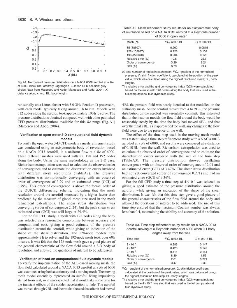
run serially on a Linux cluster with 3.0GHz Pentium D processors,with each model typically taking around 3h to run. Models with512 nodes along the aerofoil took approximately 100h to solve. Thepressure distributions obtained compared well with other publishedCFD pressure distributions available for this Re range (Fig.A1)(Mateescu and Abdo, 2004).

Verification of open water 3-D computational fluid dynamicmodels

To verify the open water 3-D CFD models a mesh refinement studywas conducted using an axisymmetric body of revolution basedon a NACA 0013 aerofoil, in a uniform flow at a Re of 6000.Three different meshes were used with 85, 128 and 192 nodesalong the body. Using the same methodology as the 2-D case,Richardson extrapolation was used to calculate the observed orderof convergence and to estimate the discretisation errors involvedwith different mesh resolutions (TableA2). The pressuredistribution was asymptotically converging with an observedorder of convergence of 3.29 and an estimated error (GCI) of6.79%. This order of convergence is above the formal order ofthe QUICK differencing scheme, indicating that the meshresolution around the aerofoil increased by a higher factor thanpredicted by the measure of global mesh size used in the meshrefinement calculations. The shear stress distribution wasconverging (order of convergence 2. 24), but the peak shear stressestimated error (GCI) was still large at 29.4%.

For the full CFD study, a mesh with 128 nodes along the bodywas selected as a reasonable compromise between accuracy andcomputational cost, giving a good estimate of the pressuredistribution around the aerofoil, while giving an indication of theshape of the shear distribution. The 128-node models tookapproximately 3h to solve, and the 192-node mesh took over 60hto solve. It was felt that the 128-node mesh gave a good picture ofthe general characteristic of the flow field around a 3-D body ofrevolution and allowed the questions of interest to be addressed.

Verification of head-on computational fluid dynamic modelsTo verify the implementation of the ALE-based moving mesh, theflow field calculated around a NACA 0013 aerofoil at a Re of 6000was examined using both a stationary and a moving mesh. The movingmesh model essentially represented an aerofoil being impulsivelystarted from rest, so it was expected that it would take some time forthe transient effects of the sudden acceleration to fade. The aerofoilwas moved through 9BL and the results showed that after it had moved

4BL the pressure field was nearly identical to that modelled on thestationary mesh. As the aerofoil moved from 4 to 9BL, the pressuredistribution on the aerofoil was essentially constant. This indicatedthat in the head-on models the flow field around the body would bereasonably steady by the time the body had moved 4BL, and thatover the final 2BL, as it approached the wall, any changes to the flowfield were due to the presence of the wall.

The effect of the time step used in the moving mesh modelwas tested using a time step refinement study with a NACA 0013aerofoil at a Re of 6000, and results were compared at a distanceof 0.10BL from the wall. Richardson extrapolation was used tocalculate the observed order of convergence and to estimate thediscretisation errors involved with the size of the time step(TableA3). The pressure distribution showed oscillatingconvergence with an observed order of convergence of 2.01 andan estimated error (GCI) of 3.47%. The shear stress distributionhad not yet converged (order of convergence 0.271) and had anestimated error (GCI) of 9.36%.

For the full CFD study a time step of 4�10–4 was selected asgiving a good estimate of the pressure distribution around theaerofoil, while giving an indication of the shape of the sheardistribution. It was felt that this time step gave a good picture ofthe general characteristics of the flow field around the body andallowed the questions of interest to be addressed. The use of thistime step ensured that the maximum Courant number was alwaysless than 0.4, maintaining the stability and accuracy of the solution.


Table A2. Mesh refinement study results for an axisymmetric bodyof revolution based on a NACA 0013 aerofoil at a Reynolds number

of 6000 in open water

Mesh (N) �CP at 0.5 BL Cf at 0.02 BL

85 (38507) 0.202 0.0815128 (102897) 0.226 0.109196 (276870) 0.234 0.123Relative error (%) 10.5 25.5Order of convergence 3.29 2.24GCI (%) 6.79 29.4

N, total number of nodes in each mesh; �CP, gradient of the normalisedpressure; Cf, skin friction coefficient, calculated at the position of the peakvalue, which was calculated using the highest resolution mesh; BL, bodylengths.

The relative error and the grid convergence index (GCI) were calculatedbased on the mesh with 128 nodes along the body that was used in thefull computational fluid dynamics study.

Table A3. Time step refinement study results for a NACA 0013aerofoil moving at a Reynolds number of 6000 when 0.1 body

lengths away from the wall

Time step �CP at 0.5 BL Cf at 0.016 BL

8�10–4 0.385 0.1474�10–4 0.420 0.1492�10–4 0.411 0.151Relative error (%) 8.39 1.55Order of convergence 2.01 0.271GCI (%) 3.47 9.36

�CP, gradient of the normalised pressure; Cf, skin friction coefficient,calculated at the position of the peak value, which was calculated usingthe highest resolution time step; BL, body lengths.

The relative error and the grid convergence index (GCI) were calculatedbased on the 4�10–4 time step that was used in the full computationalfluid dynamics study.

0 0.1 0.2 0.3 0.4 0.5 0.6 0.7 0.8 0.9 1

−0.4

−0.3

−0.2

−0.1

0

0.1

0.2

0.3

0.4

0.5

X (BL)

C

P

Fig.A1. Normalised pressure distribution on a NACA 0008 aerofoil at a Reof 6000. Black line, arbitrary Lagrangian–Eulerian CFD solution; greycircles, data from Mateescu and Abdo (Mateescu and Abdo, 2004). X,distance along chord; BL, body length.



LIST OF SYMBOLS AND ABBREVIATIONSALE arbitrary Lagrangian–Eulerian BL body lengthCFD computational fluid dynamicsCf skin friction coefficientCP coefficient of pressureP pressure fieldPIV particle image velocimetryRe Reynolds numberu velocity fieldut tangential velocityU swimming speed of the fishUnorm normalised velocity fieldy direction normal to the surfaceDCP normalised pressure difference across canal pores�CP gradient of the normalised pressure the dynamic viscosity of the fluid the density of the fluidw wall shear stress

REFERENCESAbdo, M. (2005). Low-Reynolds number aerodynamics of airfoils at incidence. In 3rd

AIAA Aerospace Sciences Meeting and Exhibit. Reno, Nevada: American Institute ofAeronautics and Astronautics.

Anderson, J. D. (1995). Computational Fluid Dynamics: the Basics with Applications.New York, Bogotá: McGraw-Hill.

Cameron, S. M. (2007). Near-Boundary Flow Structure and Particle Entrainment. PhDThesis, University of Auckland, NZ.

Celik, I. B. (2008). Procedure for estimation and reporting of uncertainty due todiscretization in CFD applications. J. Fluid. Eng. 130, 078001.

Coombs, S. and Montgomery, J. C. (1999). The enigmatic lateral line system. InComparative Hearing: Fish and Amphibians (ed. R. R. Fay and A. N. Popper), pp.319-362. New York: Springer-Verlag.

Denton, E. J. and Gray, J. (1983). Mechanical factors in the excitation of clupeidlateral lines. Proc. R. Soc. Lond. B. Biol. Sci. 218, 1-26.

Denton, E. J. and Gray, J. (1988). Mechanical factors in the excitation of the lateralline of fishes. In Sensory Biology of Aquatic Animals (ed. J. Atema, R. R. Fay, A. N.Popper and W. N. Tavolga), pp. 595-618. New York: Springer-Verlag.

Dijkgraaf, S. (1963). Functioning and significance of lateral-line organs. Biol. Rev.Camb. Philos. Soc. 38, 51-105.

Drucker, E. G. and Lauder, G. V. (2002). Experimental hydrodynamics of fishlocomotion: Functional insights from wake visualization. Integr. Comp. Biol. 42, 243-257.

Dubois, A. B., Cavagna, G. A. and Fox, R. S. (1974). Pressure distribution on bodysurface of swimming fish. J. Exp. Biol. 60, 581-591.

Fujisawa, N., Nakamura, K. and Srinivas, K. (2004). Interaction of two parallel planejets of different velocities. J. Visual. 7, 135-142.

Fujisawa, N., Tanahashi, S. and Srinivas, K. (2005). Evaluation of pressure field andfluid forces on a circular cylinder with and without rotational oscillation using velocitydata from PIV measurement. Meas. Sci. Technol. 16, 989-996.

Fujisawa, N., Nakamura, Y., Matsuura, F. and Sato, Y. (2006). Pressure fieldevaluation in microchannel junction flows through mu PIV measurement.Microfluidics and Nanofluidics 2, 447-453.

Gorner, P. (1963). Untersuchungen zur morphologie und elektrophysiologie desseitenlinienorgans vom krallenfrosch (Xenopus laevis Daudin). Zeitschrift FurVergleichende Physiologie 47, 316-338.

Gurka, R., Liberzon, A., Hefetz, D., Rubinstein, D. and Shavit, U. (1999).Computation of pressure distribution using PIV velocity data. In Proceedings of theThird International Workshop PIV, pp. 671-676. Santa Barbara.

Harlow, F. H. and Welch, J. E. (1965). Numerical calculation of time-dependentviscous incompressible flow of fluid with free surface. Phys. Fluids 8, 2182-2189.

Hassan, E. S. (1985). Mathematical-analysis of the stimulus for the lateral line organ.Biol. Cybern. 52, 23-36.

Hassan, E. S. (1989). Hydrodynamic imaging of the surroundings by the lateral line ofthe blind cave fish Anoptichthys jordani. In The Mechanosensory Lateral Line:Neurobiology and Evolution (ed. S. Coombs, P. Gorner and H. Munz), pp. 217-228.New York: Springer-Verlag.

Hassan, E. S. (1992a). Mathematical-description of the stimuli to the lateral line systemof fish derived from a 3-dimensional flow field analysis: I. The cases of moving in openwater and of gliding towards a plane surface. Biol. Cybern. 66, 443-452.

Hassan, E. S. (1992b). Mathematical-description of the stimuli to the lateral linesystem of fish derived from a 3-dimensional flow field analysis: II. The case of glidingalongside or above a plane surface. Biol. Cybern. 66, 453-461.

Hirt, C. W., Amsden, A. A. and Cook, J. L. (1974). An arbitrary Lagrangian-Euleriancomputing method for all flow speeds. J. Comput. Phys. 14, 227-253.

Hosokawa, S., Moriyama, S., Tomiyama, A. and Takada, N. (2003). PIVmeasurement of pressure distributions about single bubbles. J. Nucl. Sci. Technol.40, 754-762.

Jielof, R., Spoor, A. and Devries, H. (1952). The microphonic activity of the lateralline. J. Physiol. Lond. 116, 137-157.

Kalmijn, A. J. (1988). Hydrodynamic and acoustic field detection. In Sensory Biologyof Aquatic Animals (eds J. Atema, R. R. Fay, A. N. Popper and W. N. Tavolga), pp.83-130. New York: Springer-Verlag.

Kalmijn, A. J. (1989). Functional evolution of lateral line and inner ear sensorysystems. In The Mechanosensory Lateral Line: Neurobiology and Evolution (eds S.Coombs, P. Gorner and H. Munz), pp. 187-216. New York: Springer-Verlag.

Kroese, A. B. A. and Schellart, N. A. M. (1992). Velocity-sensitive and acceleration-sensitive units in the trunk lateral line of the trout. J. Neurophysiol. 68, 2212-2221.

Kroese, A. B. A., Vanderzalm, J. M. and Vandenbercken, J. (1978). Frequency-response of lateral-line organ of Xenopus laevis. Pflugers Arch. Eur. J. Physiol. 375,167-175.

Kuiper, J. W. (1967). Frequency characteristics and functional significance of thelateral line organ. In Lateral Line Detectors (ed. P. H. Cahn), pp. 105-121.Bloomington: Indiana University Press.

Kunz, P. J. and Kroo, I. (2001). Analysis and design of airfoils for use at ultra-lowReynolds numbers. In Fixed and Flapping Wing Aerodynamics For Micro Air VehicleApplications, Vol. 195 (ed. T. J. Mueller), pp. 35-60. Reston, VA: American Instituteof Aeronautics and Astronautics.

Leonard, B. P. (1979). Stable and accurate convective modeling procedure based onquadratic upstream interpolation. Comput. Meth. Appl. Mech. Eng. 19, 59-98.

Leonard, B. P. (1988). Elliptic systems: finite-difference method IV. In Handbook ofNumerical Heat Transfer (eds W. J. Minkowycz, E. M. Sparrow, G. E. Schneider andR. H. Pletcher), pp. 347–378. New York: Wiley.

Mateescu, D. and Abdo, M. (2004). Aerodynamic analysis of airfoils at very lowReynolds numbers. In 42nd AIAA Aerospace Sciences Meeting and Exhibit, pp.6341-6351. Reno, NV, USA: American Institute of Aeronautics and AstronauticsIncorporated, Reston.

McHenry, M. J., Strother, J. A. and van Netten, S. M. (2008). Mechanical filtering bythe boundary layer and fluid-structure interaction in the superficial neuromast of thefish lateral line system. J. Comp. Physiol. A 194, 795-810.

Murai, Y., Nakada, T., Suzuki, T. and Yamamoto, F. (2007). Particle trackingvelocimetry applied to estimate the pressure field around a Savonius turbine. Meas.Sci. Technol. 18, 2491-2503.

Norris, S. E., Were, C. J., Richards, P. J. and Mallinson, G. D. (2010). A Voronoibased ALE solver for the calculation of incompressible flow on deformingunstructured meshes. Int. J. Numer. Meth. Fluid. Epub ahead of print.

Partridge, B. L. and Pitcher, T. J. (1980). The sensory basis of fish schools - relativeroles of lateral line and vision. J. Comp. Physiol. 135, 315-325.

Patankar, S. V. and Spalding, D. B. (1972). Calculation procedure for heat, mass andmomentum-transfer in 3-dimensional parabolic flows. Int. J. Heat Mass Transf. 15,1787-1806.

Rapo, M. A., Jiang, H., Grosenbaugh, M. and Coombs, S. (2009). Usingcomputational fluid dynamics to calculate the stimulus to the lateral line of a fish instill water. J. Exp. Biol. 212, 1494-1505.

Rhie, C. M. and Chow, W. L. (1983). Numerical study of the turbulent-flow past anairfoil with trailing edge separation. AIAA J. 21, 1525-1532.

Roache, P. J. (1997). Quantification of uncertainty in computational fluid dynamics.Annu. Rev. Fluid Mech. 29, 123-160.

Schemmel, C. (1967). Vergleichende Untersuchungen an den Hautsinnesorganenober- und unterirdisch lebender Astyanax-Formen. Zeitschrift fur Morphologie derTiere 61, 255-316.

Schiffman, H. R. (1996). Sensation and Perception: an Integrated Approach. NewYork: Wiley.

Schlicke, T., Cameron, S. M. and Coleman, S. E. (2007). Galvanometer-based PIVfor liquid flows. Flow. Meas. Instrum. 18, 27-36.

Teghtsoonian, R. (1971). On the exponents in Stevens’ law and the constant inEkman’s law. Psychol. Rev. 78, 71-80.

Teyke, T. (1985). Collision with and avoidance of obstacles by blind cave fishAnoptichthys jordani (Characidae). J. Comp. Physiol. A 157, 837-843.

Teyke, T. (1988). Flow field, swimming velocity and boundary layer: parameters whichaffect the stimulus for the lateral line organ in blind fish. J. Comp. Physiol. A 163,53-61.

Teyke, T. (1989). Learning and remembering the environment in the blind cave fishAnoptichthys jordani. J. Comp. Physiol. A 164, 655-662.

Teyke, T. (1990). Morphological differences in neuromasts of the blind cave fishAstyanax hubbsi and the sighted river fish Astyanax mexicanus. Brain Behav. Evol.35, 23-30.

van Netten, S. M. (2006). Hydrodynamic detection by cupulae in a lateral line canal:functional relations between physics and physiology. Biol. Cybern. 94, 67-85.

von Campenhausen, C., Riess, I. and Weissert, R. (1981). Detection of stationaryobjects by the blind cave fish Anoptichthys jordani (Characidae). J. Comp. Physiol. A143, 369-374.

Weissert, R. and von Campenhausen, C. (1981). Discrimination between stationaryobjects by the blind cave fish Anoptichthys jordani (Characidae). J. Comp. Physiol. A143, 375-381.

Were, C. J. (1997). The Free-ALE Method for Unsteady Incompressible Flow inDeforming Geometries. PhD Thesis, University of Auckland, NZ.

White, F. M. (2006). Viscous Fluid Flow. Boston: McGraw-Hill.Windsor, S. P. (2008). Hydrodynamic Imaging by Blind Mexican Cave Fish. PhD

Thesis, University of Auckland, NZ.Windsor, S. P. and McHenry, M. J. (2009). The influence of viscous hydrodynamics

on the fish lateral-line system. Integr. Comp. Biol. 49, 691-701.Windsor, S. P., Tan, D. and Montgomery, J. C. (2008). Swimming kinematics and

hydrodynamic imaging in the blind Mexican cave fish (Astyanax fasciatus). J. Exp.Biol. 211, 2950-2959.

Windsor, S. P., Norris, S. E., Cameron, S. M., Mallinson, G. D. and Montgomery, J.C. (2010). The flow fields involved in hydrodynamic imaging by blind Mexican cave fish(Astyanax fasciatus). Part II: gliding parallel to a wall. J. Exp. Biol. 213, 3832-3842.

Wolfgang, M. J., Anderson, J. M., Grosenbaugh, M. A., Yue, D. K. P. andTriantafyllou, M. S. (1999). Near-body flow dynamics in swimming fish. J. Exp. Biol.202, 2303-2327.

Yasuda, K. (1973). Comparative studies on swimming behavior of blind cave fish andgoldfish. Comp. Biochem. Physiol. 45, 515-527.


Documents

The flow fields involved in hydrodynamic imaging by blind Mexican