Embed Size (px)
Citation preview
Paper by Eric Shen for IDS Workshop on Friday, October 23, 2009
h f ll h b l d d• The full paper has not been translated and revised in English.
• A set of slides have been prepared, some of which I will use in the presentation and some pthat are supplementary. The supplementary slides will be used for reference to respond to pquestions.
• Please read through the slides before the• Please read through the slides before the workshop.
A Sequential Group Decision Process M th d f E RMethod for Emergency Response
Eric ShenP f f IT d ISProfessor of IT and IS
Department of Management Information SystemsAnti College of Economics & Management
Shanghai Jiao Tong University, China
Eric (Huizhang) ShenEric (Huizhang) Shen
• Research on Group Decision Support of Emergency Response to Crisis Management. g y p gSupported by the National Natural Science Foundation of ChinaFoundation of China
• Research on the Diffusion and Control of Panic h l hPsychologies and Behaviors in Emergencies.
Supported by the PhD Programs Foundation of the Ministry of Education of China
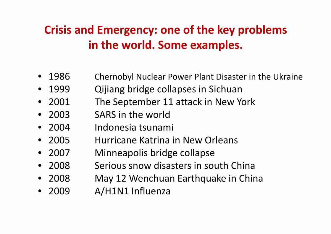
Crisis and Emergency: one of the key problems in the world. Some examples.
• 1986 Chernobyl Nuclear Power Plant Disaster in the Ukraine• 1999 Qijiang bridge collapses in Sichuan1999 Qijiang bridge collapses in Sichuan• 2001 The September 11 attack in New York• 2003 SARS in the world2003 SARS in the world• 2004 Indonesia tsunami• 2005 Hurricane Katrina in New Orleans• 2007 Minneapolis bridge collapse• 2008 Serious snow disasters in south China• 2008 May 12 Wenchuan Earthquake in China• 2009 A/H1N1 Influenza
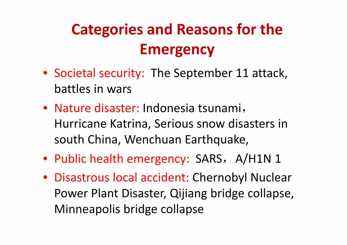
Categories and Reasons for the Emergency
• Societal security: The September 11 attack, battles in wars
• Nature disaster: Indonesia tsunami,Hurricane Katrina Serious snow disasters inHurricane Katrina, Serious snow disasters in south China, Wenchuan Earthquake,
• Public health emergency: SARS,A/H1N 1• Disastrous local accident: Chernobyl Nuclear• Disastrous local accident: Chernobyl Nuclear Power Plant Disaster, Qijiang bridge collapse, Mi li b id llMinneapolis bridge collapse
Are there commonalities in Emergencies?
• Characteristics of emergencies?
• Decision problems in emergencies ?Decision problems in emergencies ?
• What decisions can be supported by i f i ?information systems ?
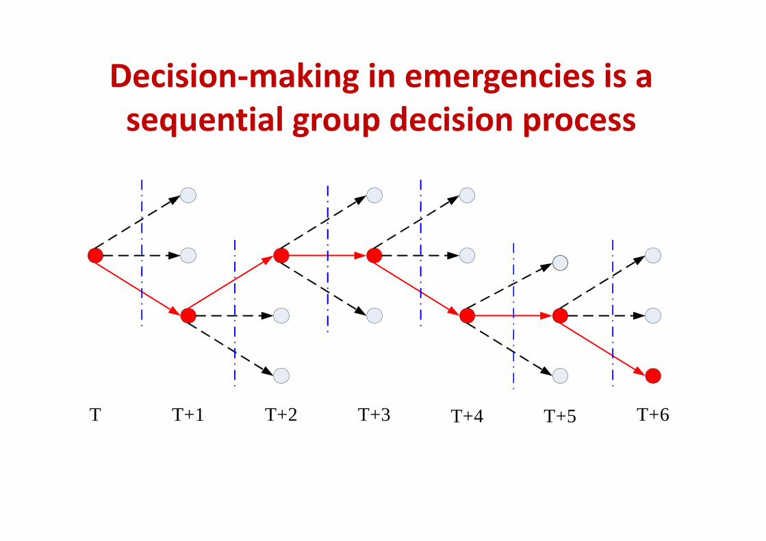
Decision‐making in emergencies is aDecision making in emergencies is a sequential group decision process
T T+1 T+2 T+3 T+4 T+5 T+6
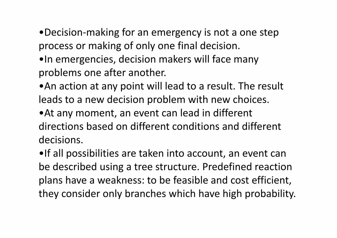
•Decision‐making for an emergency is not a one step process or making of only one final decision. •In emergencies, decision makers will face many problems one after another. •An action at any point will lead to a result. The result leads to a new decision problem with new choices. •At any moment, an event can lead in different directions based on different conditions and different decisions. •If all possibilities are taken into account, an event can be described using a tree structure. Predefined reaction plans have a weakness: to be feasible and cost efficient, they consider only branches which have high probability.
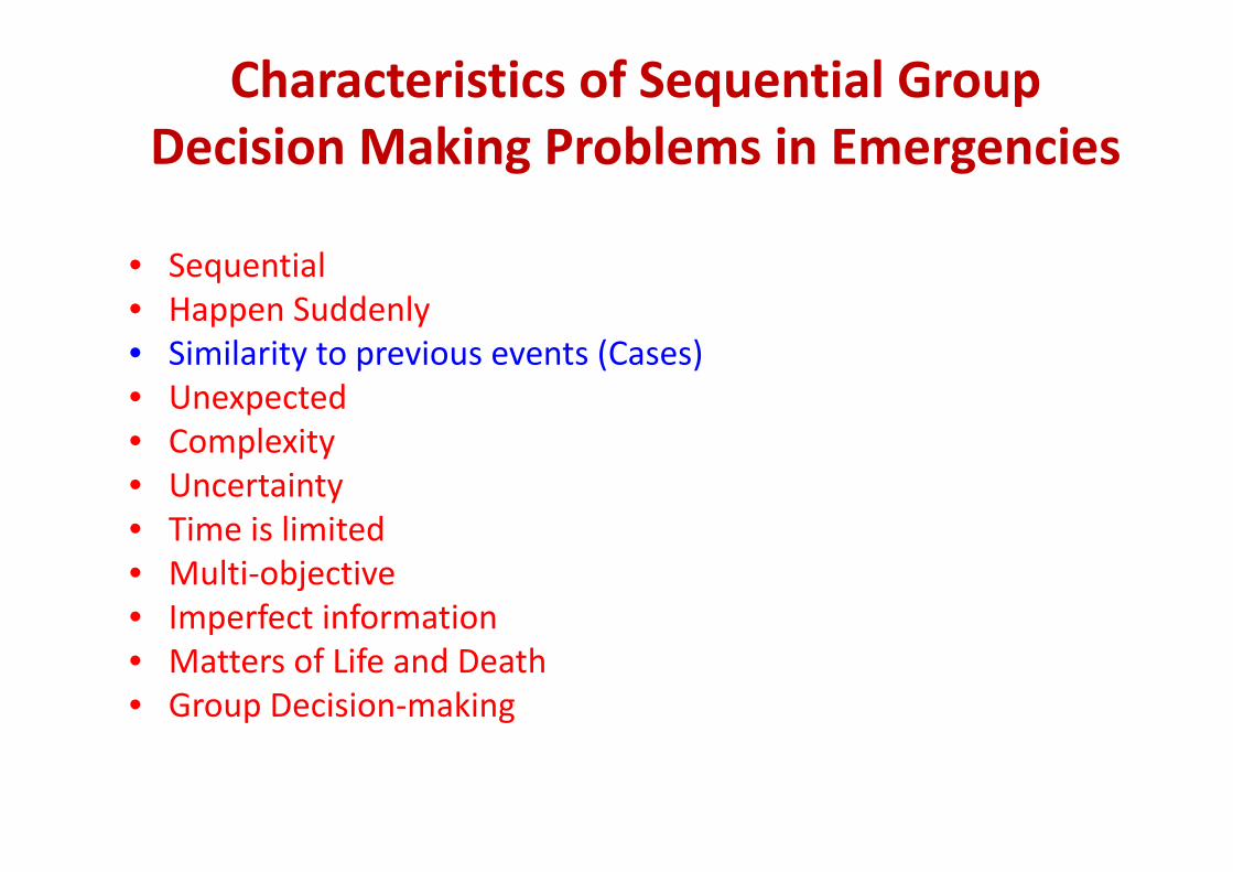
Characteristics of Sequential Group Decision Making Problems in EmergenciesDecision Making Problems in Emergencies
• Sequential• Happen Suddenly • Similarity to previous events (Cases)• Unexpected • Complexity• Complexity• Uncertainty• Time is limitedTime is limited• Multi‐objective • Imperfect information p• Matters of Life and Death • Group Decision‐making
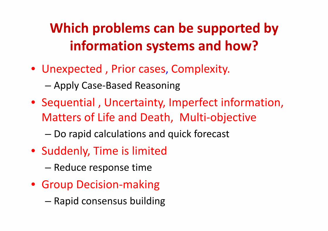
Which problems can be supported by information systems and how?
• Unexpected , Prior cases, Complexity. – Apply Case‐Based Reasoningpp y g
• Sequential , Uncertainty, Imperfect information, Matters of Life and Death Multi objectiveMatters of Life and Death, Multi‐objective – Do rapid calculations and quick forecast
• Suddenly, Time is limited– Reduce response time– Reduce response time
• Group Decision‐making– Rapid consensus building
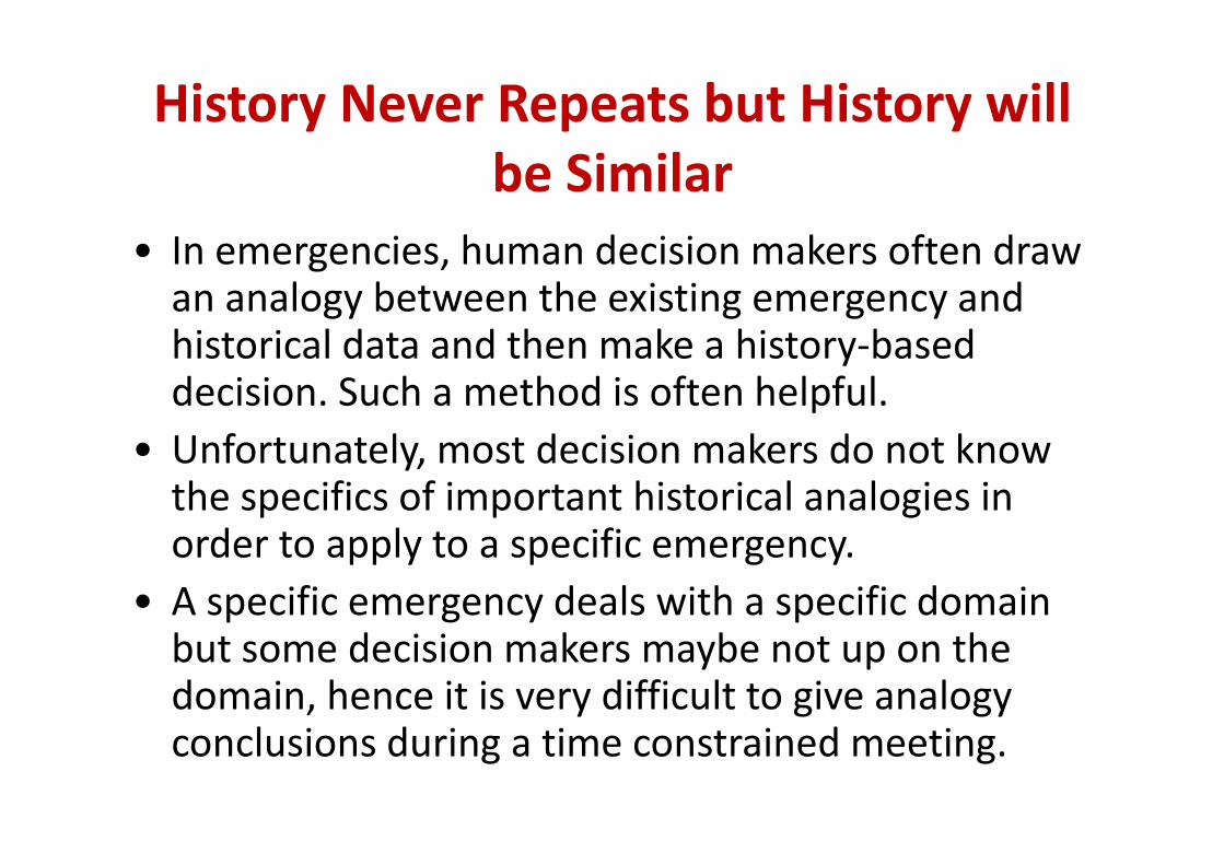
History Never Repeats but History will be Similar
i h d i i k f d• In emergencies, human decision makers often draw an analogy between the existing emergency and hi t i l d t d th k hi t b dhistorical data and then make a history‐based decision. Such a method is often helpful.
• Unfortunately, most decision makers do not know the specifics of important historical analogies in d l ifiorder to apply to a specific emergency.
• A specific emergency deals with a specific domain but some decision makers maybe not up on the domain, hence it is very difficult to give analogy
l d dconclusions during a time constrained meeting.
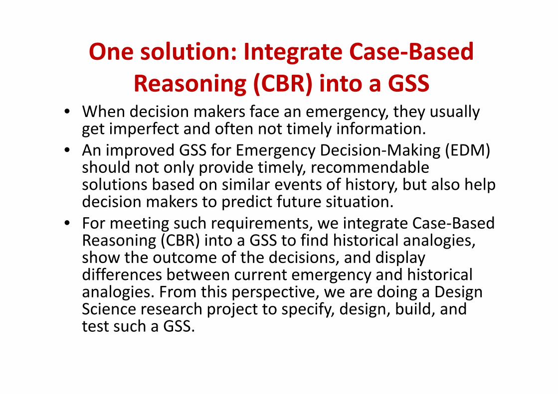
One solution: Integrate Case‐Based gReasoning (CBR) into a GSS
Wh d i i k f th ll• When decision makers face an emergency, they usually get imperfect and often not timely information.
• An improved GSS for Emergency Decision‐Making (EDM)An improved GSS for Emergency Decision Making (EDM) should not only provide timely, recommendable solutions based on similar events of history, but also help d i i k t di t f t it tidecision makers to predict future situation.
• For meeting such requirements, we integrate Case‐Based Reasoning (CBR) into a GSS to find historical analogiesReasoning (CBR) into a GSS to find historical analogies, show the outcome of the decisions, and display differences between current emergency and historical
l i F hi i d i D ianalogies. From this perspective, we are doing a Design Science research project to specify, design, build, and test such a GSS.test such a GSS.
A Classic Emergency Response Situation is a Battle in a War
• The Battle of Midway is an interesting study of emergency response in a battle. g y p
• The Battle of Midway is a good case study because there are lots of detailed reportsbecause there are lots of detailed reports.
• The Battle of Midway has many characteristics that are common to emergency.
Case‐Based Examples (Analogies) f lcome from History—War examples
• The Art of War (Chinese: pinyin: Sūn Zǐ Bīng Fǎ) is one ( p y g )of the oldest and most successful books on military strategy. It was written by Sun Tzu in the 6th century BC. gy y yIt is still one of the textbooks at West Point.
• Sun Tzu thought that strategy was not planning in theSun Tzu thought that strategy was not planning in the sense of working through an established list, but rather that it requires quick and appropriate responses tothat it requires quick and appropriate responses to changing conditions. Planning works in a controlled environment, but in a changing environment, competingenvironment, but in a changing environment, competing plans collide, creating unexpected situations.
The Art of War (2)The Art of War (2)
Another book the Zuo Zhuan ( pinyin: zuǒzhuàn), translated as the Chronicle of Zuo or )the Commentary of Zuo, is the earliest Chinese work of narrative history and coversChinese work of narrative history and covers the period from 722 BCE to 468 BCE.
It present war history as cases. h h iThese cases are short stories.
Case–based Advise from Art of War that apply in the Battle of Midway
• All d d i tt k th l th t ill b• All we need do is attack some other place that enemy will be obliged to relieve.
• Know the enemy and know yourself.
• Don't spread out your forces! Concentrate your attacks on oneDon t spread out your forces! Concentrate your attacks on one target at a time!
• Pride will lead to a fall• Pride will lead to a fall
• Be constantly on the alert to not be taken by surprise.
• Attack in order to defend.
Battle of Midway as an Emergency Response
Time=T=Mar 1942 (1)Time=T=Mar 1942 (1)
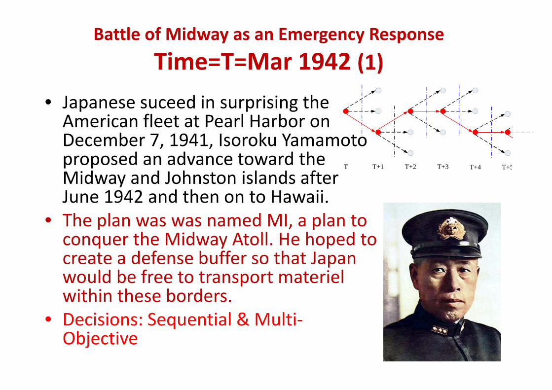
• Japanese suceed in surprising theJapanese suceed in surprising the American fleet at Pearl Harbor on December 7, 1941, Isoroku Yamamoto proposed an advance toward the Midway and Johnston islands after June 1942 and then on to Hawaii
T T+1 T+2 T+3 T+4 T+5
June 1942 and then on to Hawaii. • The plan was was named MI, a plan to conquer the Midway Atoll He hoped toconquer the Midway Atoll. He hoped to create a defense buffer so that Japan would be free to transport materiel pwithin these borders.
• Decisions: Sequential & Multi‐qObjective
Time=T=Mar 1942 (2)Time=T=Mar 1942 (2)
' l d b• Yamamoto's plan was not supported by everyone.
• The Headquarters and the top Navy leaders looked more toward the South Pacific as the next step of conquest, looking to seal off Australia (a potential American base) by ( p ) ypushing toward New Caledonia, Fiji, and Samoa.Samoa.
• Group Decision‐making & Multi‐objective
Time=T+1= April and May 1942 (1)Time=T+1= April and May 1942 (1)
• The Doolittle Raid, 18 April 1942, was the first air raid by the United States to strike a yJapanese home island. The raid caused everyone to support plan MI (main strike ateveryone to support plan MI (main strike at Midway with diversion attack on Alaska Aleutian IslandsAleutian Islands.
• The Pacific military balance between Japanese and United States is as follow:
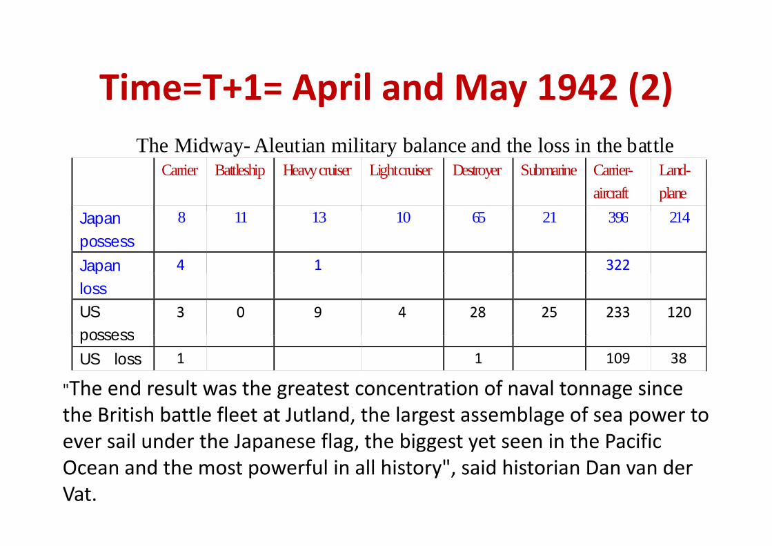
Time=T+1= April and May 1942 (2)Time=T+1= April and May 1942 (2)The Midway- Aleutian military balance and the loss in the battleThe Midway Aleutian military balance and the loss in the battle
Carrier Battleship Heavy cruiser Light cruiser Destroyer Submarine Carrier- aircraft
Land- plane
Japan possess
8 11 13 10 65 21 396 214
Japan 4 1 322 ploss US possess
3 0 9 4 28 25 233 120
"The end result was the greatest concentration of naval tonnage since
possessUS loss 1 1 109 38
g gthe British battle fleet at Jutland, the largest assemblage of sea power to ever sail under the Japanese flag, the biggest yet seen in the Pacific Ocean and the most powerful in all history", said historian Dan van der Vat.
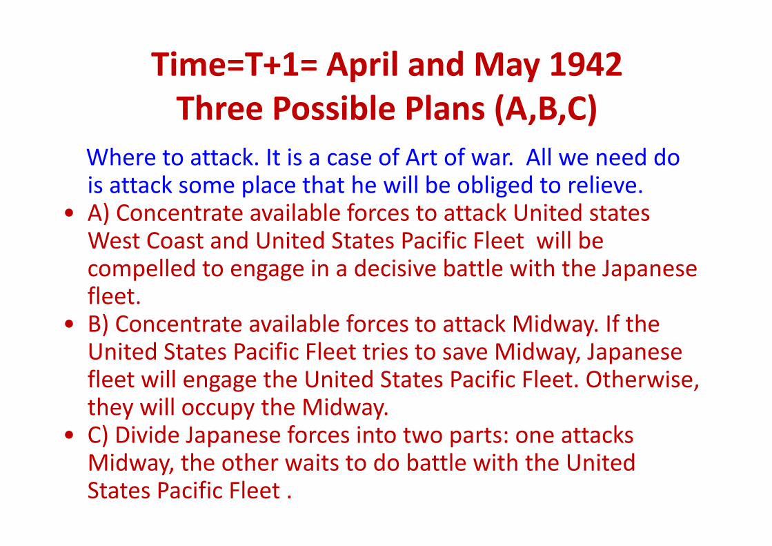
Time=T+1= April and May 1942Three Possible Plans (A,B,C)
Wh k I i f A f All d dWhere to attack. It is a case of Art of war. All we need do is attack some place that he will be obliged to relieve.
• A) Concentrate available forces to attack United states• A) Concentrate available forces to attack United states West Coast and United States Pacific Fleet will be compelled to engage in a decisive battle with the Japanesecompelled to engage in a decisive battle with the Japanese fleet.
• B) Concentrate available forces to attack Midway. If the ) yUnited States Pacific Fleet tries to save Midway, Japanese fleet will engage the United States Pacific Fleet. Otherwise, they will occupy the Midway.
• C) Divide Japanese forces into two parts: one attacks Midway the other waits to do battle with the UnitedMidway, the other waits to do battle with the United States Pacific Fleet .
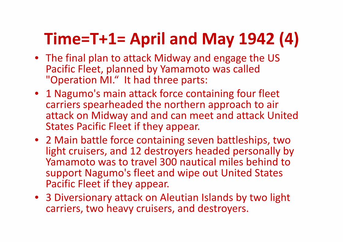
Time=T+1= April and May 1942 (4)Time=T+1= April and May 1942 (4)• The final plan to attack Midway and engage the US P ifi Fl t l d b Y t ll dPacific Fleet, planned by Yamamoto was called "Operation MI.“ It had three parts:
• 1 Nagumo's main attack force containing four fleet• 1 Nagumo s main attack force containing four fleet carriers spearheaded the northern approach to air attack on Midway and and can meet and attack United States Pacific Fleet if they appear.
• 2 Main battle force containing seven battleships, two li ht i d 12 d t h d d ll blight cruisers, and 12 destroyers headed personally by Yamamoto was to travel 300 nautical miles behind to support Nagumo's fleet and wipe out United Statessupport Nagumo s fleet and wipe out United States Pacific Fleet if they appear.
• 3 Diversionary attack on Aleutian Islands by two light carriers, two heavy cruisers, and destroyers.
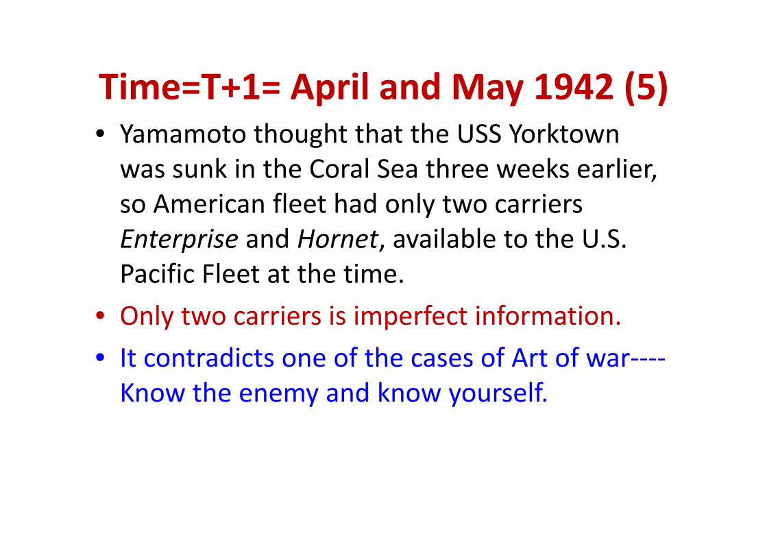
Time=T+1= April and May 1942 (5)Time=T+1= April and May 1942 (5)• Yamamoto thought that the USS Yorktown was sunk in the Coral Sea three weeks earlier, so American fleet had only two carriersso American fleet had only two carriers Enterprise and Hornet, available to the U.S. Pacific Fleet at the timePacific Fleet at the time.
• Only two carriers is imperfect information.
• It contradicts one of the cases of Art of war‐‐‐‐Know the enemy and know yourselfKnow the enemy and know yourself.
Time=T+1= April and May 1942 (6)Time=T+1= April and May 1942 (6)
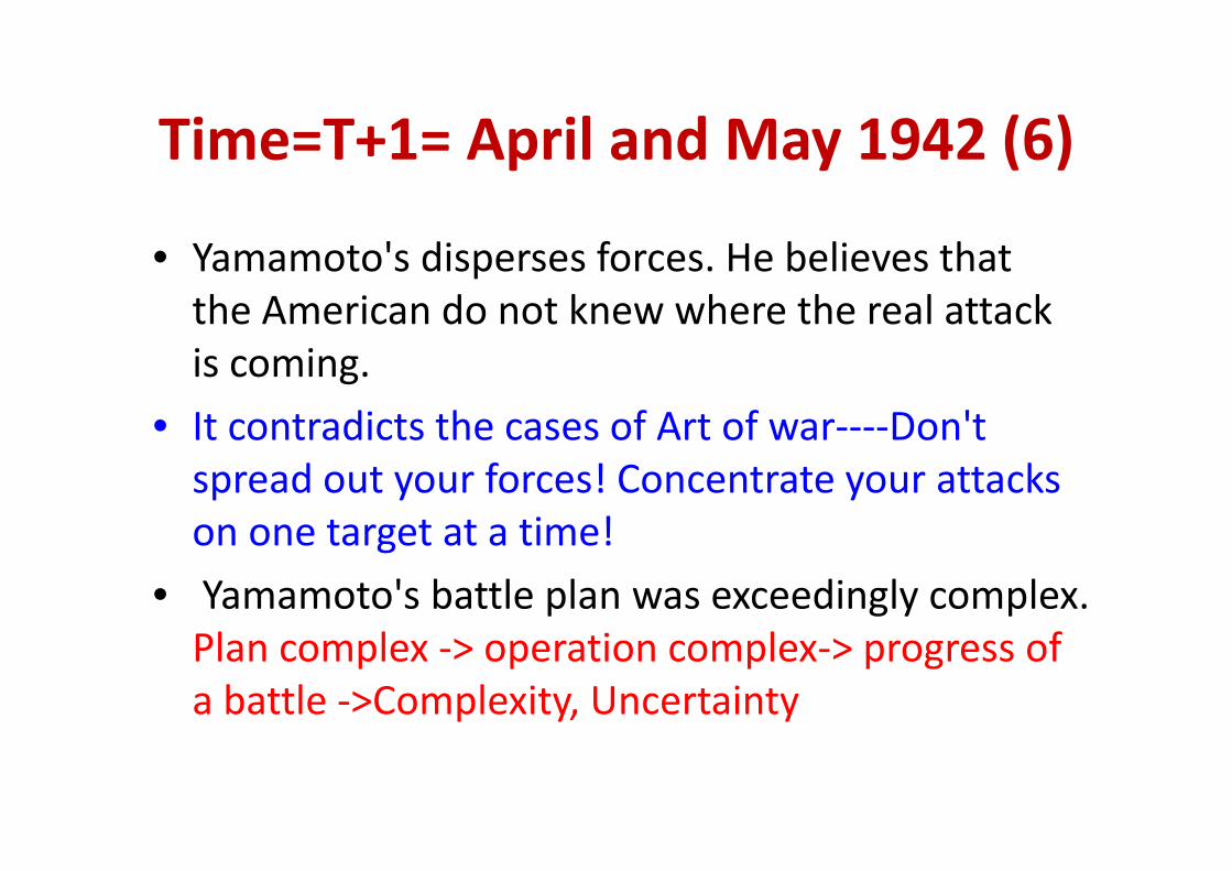
• Yamamoto's disperses forces. He believes that the American do not knew where the real attack is coming.
• It contradicts the cases of Art of war‐‐‐‐Don'tIt contradicts the cases of Art of war Don t spread out your forces! Concentrate your attacks on one target at a time!on one target at a time!
• Yamamoto's battle plan was exceedingly complex. l l i l fPlan complex ‐> operation complex‐> progress of
a battle ‐>Complexity, Uncertainty
Time=T+1= April and May 1942 (7)Time=T+1= April and May 1942 (7)
O M 27 1942 th t d il d f th• On May 27, 1942 the great armada sailed from the fleet anchorage in the Inland Sea of Japan. That day was the Navy Day ‐ anniversary of the great victorywas the Navy Day anniversary of the great victory of Japan over Russia in the Battle of Tsushima, during the Russo‐Japanese war. Japanese were g p pconfident that this sortie would end in success also. They knew that the weakened American fleet had
l t i t h d h i i donly two carriers at hand, whose inexperienced pilots had no chance to win against their more numerous and more experienced foenumerous and more experienced foe.
• It contradicts one of the cases of Art of war‐‐‐‐ Pride Will Have a FallWill Have a Fall
Time=T+1= April and May 1942 (8)Time=T+1= April and May 1942 (8)
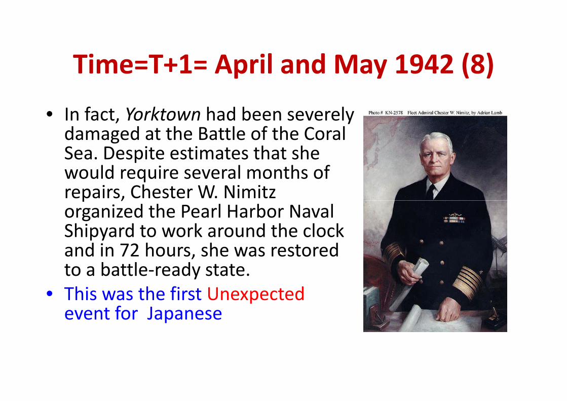
I f t Y kt h d b l• In fact, Yorktown had been severely damaged at the Battle of the Coral Sea Despite estimates that sheSea. Despite estimates that she would require several months of repairs, Chester W. Nimitz p ,organized the Pearl Harbor Naval Shipyard to work around the clock d i 72 h h t dand in 72 hours, she was restored
to a battle‐ready state.• This was the first Unexpected• This was the first Unexpectedevent for Japanese
Time=T+1= April and May 1942 (9)The second Unexpected for JapaneseThe second Unexpected for Japanese
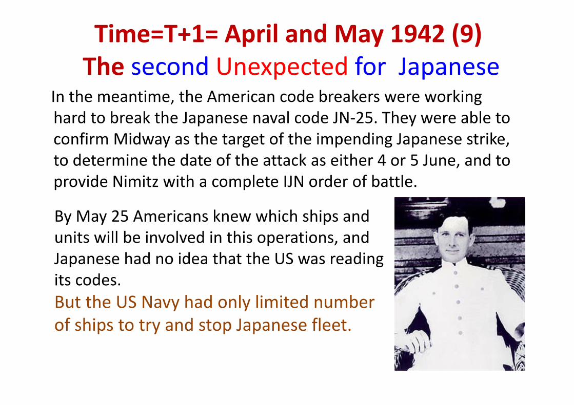
In the meantime, the American code breakers were working hard to break the Japanese naval code JN‐25. They were able to confirm Midway as the target of the impending Japanese strike, t d t i th d t f th tt k ith 4 5 J d tto determine the date of the attack as either 4 or 5 June, and to provide Nimitz with a complete IJN order of battle.
By May 25 Americans knew which ships and units will be involved in this operations, and Japanese had no idea that the US was reading its codes.But the US Navy had only limited number of ships to try and stop Japanese fleet.
Time=T+2= At exactly 04:00 Jun 4 1942(1)Time=T+2= At exactly 04:00 Jun 4 1942(1)
Japanese submarine do not find US carriers Actually USJapanese submarine do not find US carriers. Actually, US carriers had passed. Nagumo could make one of three decision:decision:A) Send scout planes to search for possible US fleet, after receipt of the report from scout plane then give ordersreceipt of the report from scout plane, then give orders.b) Send scout planes to search for possible US fleet, at the same time two carriers attack Midway and twothe same time, two carriers attack Midway and two carriers wait to deal with American fleet, if it showed up. C) Send scout planes to search for possible US fleet AtC) Send scout planes to search for possible US fleet. At the same time, all four carriers with their planes attack MidwayMidway

Time=T+2= At exactly 04:00 Jun 4 1942(2)Nagumo selected the last one. Total of 144 planes took off as a part of the strikeplanes took off as a part of the strike against Midway. Each of four carriers contributed 9 fighters while the rest were b bbombers.
• Imperfect information‐‐submarine had not supplied right information (US fleet hadsupplied right information. (US fleet had passed when submarine arrived at the sea area)
• Uncertainty‐‐do not know whether scout planes have found the US fleet.
• Time is limited Japanese fleet was already• Time is limited ‐‐Japanese fleet was already near Midway.
• Multi‐objective ‐‐ attack Midway protectMulti objective attack Midway, protect against US planes, and attack US fleet.
Time=T+3= At exactly 7:15 Jun 4 1942(1)Time=T+3= At exactly 7:15 Jun 4 1942(1)
American bombers based on Midway made several attacks on the yJapanese carrier fleet. This experience may well have contributed to Nagumo's determination to launch another attack on Midway. At about this time Nagumo got advice asking for the second strike. He still had no indication of the presence of any American surface force. Nagumo had three possible decisionsNagumo had three possible decisions.
A) Keep on going as planned with planes from all carriers. ) p g g p pB) Order two carriers with their planes to be re‐armed with bombs to attack Midway, and two carriers with their planes to be in
d d h d f hreserve and armed with torpedoes for use against the American fleet, if it showed up.C) Change Plan B to have reserve planes re‐armed with bombs toC) Change Plan B to have reserve planes re‐armed with bombs to attack Midway.
Time=T+3= At exactly 7:15 Jun 4 1942(2)Nagumo selected decision 3 to rearm reserve planes to attack Midwayreserve planes to attack Midway
l d d d l• Nagumo selected decision 3 in direct violation of Yamamoto's order that the carrier force should keep its reserve strike force armed for anti‐ship operations.anti ship operations.
• Decision contradicts the cases of Art of war‐‐‐‐Th l h l bThey were constantly on the alert not to be taken by surprise.
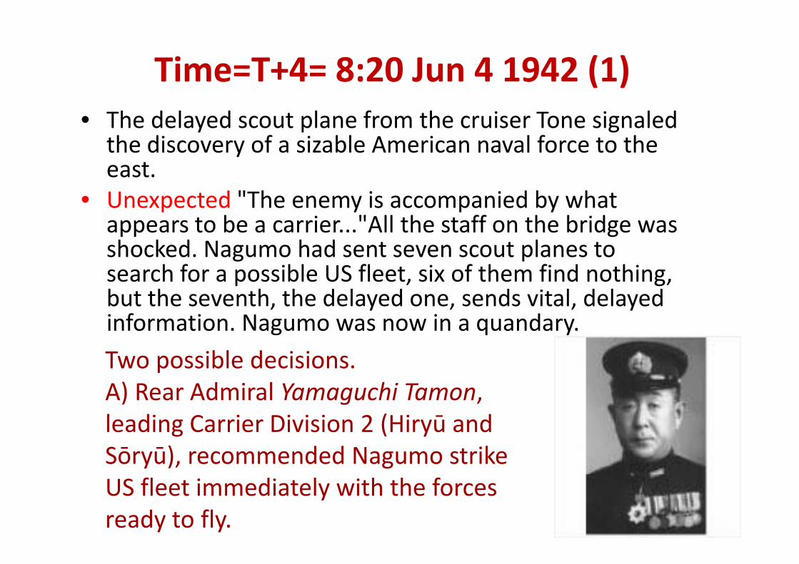
Time=T+4= 8:20 Jun 4 1942 (1)• The delayed scout plane from the cruiser Tone signaled the discovery of a sizable American naval force to the yeast.
• Unexpected "The enemy is accompanied by what t b i "All th t ff th b idappears to be a carrier..."All the staff on the bridge was
shocked. Nagumo had sent seven scout planes to search for a possible US fleet, six of them find nothing, p , g,but the seventh, the delayed one, sends vital, delayed information. Nagumo was now in a quandary.
Two possible decisions.A) Rear Admiral Yamaguchi Tamon, leading Carrier Division 2 (Hiryū and Sōryū), recommended Nagumo strike US fleet immediately with the forces ready to fly.
Time=T+4= 8:20 Jun 4 1942 (2)Evaluating the Proposed Decision AAd t• Advantages
• Seize the chance of winning a battle.• Attack in order to defend‐‐‐‐ It is a case of Art of war• Attack in order to defend‐‐‐‐ It is a case of Art of war.• To avoid being attacked by US planes.• Disadvantagessad a ages• No fighter screen, so many bombers will be lost. • If launch bombers to attack US fleet at the time, the planes that
i b k f th tt k Mid b fwere coming back from the attack on Midway, because of a shortage of fuel, will not make it to the carriers.
• The planes ready to go are armed with bombs but not torpedoes. p y g pIn attacking the US fleet, torpedoes are much better than bombs.
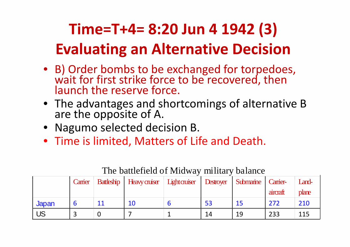
Time=T+4= 8:20 Jun 4 1942 (3)Evaluating an Alternative Decision
• B) Order bombs to be exchanged for torpedoes• B) Order bombs to be exchanged for torpedoes, wait for first strike force to be recovered, then launch the reserve force.
• The advantages and shortcomings of alternative B are the opposite of A.N l d d i i B• Nagumo selected decision B.
• Time is limited, Matters of Life and Death.
The battlefield of Midway military balanceC i B l hi H i Li h i D S b i C i L d Carrier Battleship Heavy cruiser Light cruiser Destroyer Submarine Carrier-
aircraft Land- plane
Japan 6 11 10 6 53 15 272 210
US 3 0 7 1 14 19 233 115
Time=T+5= 9: 18 Jun 4 1942Proceed with Decision B
Pl f th Mid t ik dPlanes from the Midway strike were recovered, and the whole Japanese fleet changed its course to 070 degrees to close in with the American fleetto 070 degrees to close in with the American fleet. The planes from the second wave were readied for attack on the US fleet. Planes were brought gfrom hangars to the flight deck, fully fueled and armed. The bombs that were taken off were not t d t th b b t b d th freturned to the bomb storage aboard the four
Japanese carriers; they were left lying all over the hangar deckhangar deck.
Time=T+5= 10: 22 Jun 4 1942Decision B Turns out Badly
• Japanese were totally surprised when lookouts spotted enemy• Japanese were totally surprised when lookouts spotted enemy dive bombers in a dive. It was too late for Japanese to do anything now. The dive bombers released their bombs from y g1,800 to 2,500 feet. The first three bombs missed. A fourth bomb hit, and in an instant turned the whole flight deck into a holocaust! Full of armed and fueled planes, the flight deck of the Kaga burst into flames.
I l th i t th US di b b d VB 6• In only three minutes, three US dive bomber squadrons, VB‐6, VS‐6 and VS‐3, sealed the fates of three Japanese fleet carriers and turned the tide of the whole war!and turned the tide of the whole war!
• Suddenly, Time is limited
The Design of a CBR‐Based Sequential Group Decision Process
Th d i i i ti l it ti• The group decision process in a sequential, iterative form is shown in Figure .
• The support system first presents decision makers with• The support system first presents decision makers with recommendations based on limited information.
• Then, decision makers iteratively interact with theThen, decision makers iteratively interact with the system, and estimate future events supported by the State Prediction Model component.
• With estimating result taken into account, the system sorts solutions by comparison with the real situation. O l t i f ti ti f db k• Once supplementary information or reaction feedback arrives, the new information initiate another round of decision making.dec s o a g
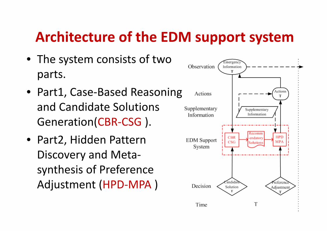
Architecture of the EDM support systemArchitecture of the EDM support system • The system consists of two e syste co s sts o t oparts.
P t1 C B d R i• Part1, Case‐Based Reasoning and Candidate Solutions Generation(CBR‐CSG ).
• Part2 Hidden PatternPart2, Hidden Pattern Discovery and Meta‐synthesis of Preferencesynthesis of Preference Adjustment (HPD‐MPA )
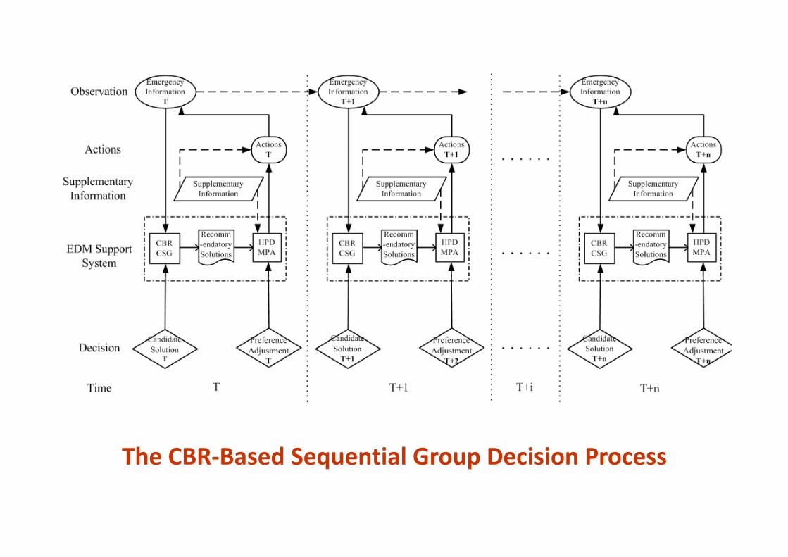
The CBR‐Based Sequential Group Decision Processq p
The CBR based sequential group decisionThe CBR‐based sequential group decisionprocess consists of n stages from “time” T to T+n‐1 h i di id d i i l h i1. Each stage is divided into six layers. The Timelayer denotes that decision makers implement around of group decision‐making for a specificemergency with the assistant of EDM supportemergency with the assistant of EDM supportsystem. The Decision layer describes aninteractive process between decision makers andinteractive process between decision makers andthe system. Decision makers should finish two
k O i i i f dtasks. One is estimating future events andproposing candidate solutions. The other isadjusting preferences to achieve consensus.
The EDM support system layer is organizedby CBR CSG (Case‐Based Reasoning andby CBR CSG (Case Based Reasoning andCandidate Solutions Generation) and HPDMPA (Hidden Patter Discovery and MetaMPA (Hidden Patter Discovery and Meta‐synthesis of Preference Adjustment). TheSupplemental Information layer is additionalinformation and data acquired during theevolution of the emergency. The Actions layeris a set of activities which implement theis a set of activities which implement theselected solution. The Observation layer isobjective events for the emergencyobjective events for the emergency.
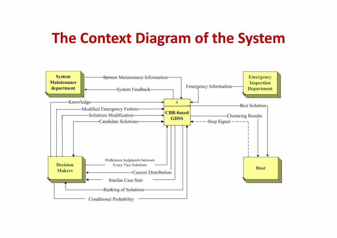
The Context Diagram of the SystemThe Context Diagram of the System
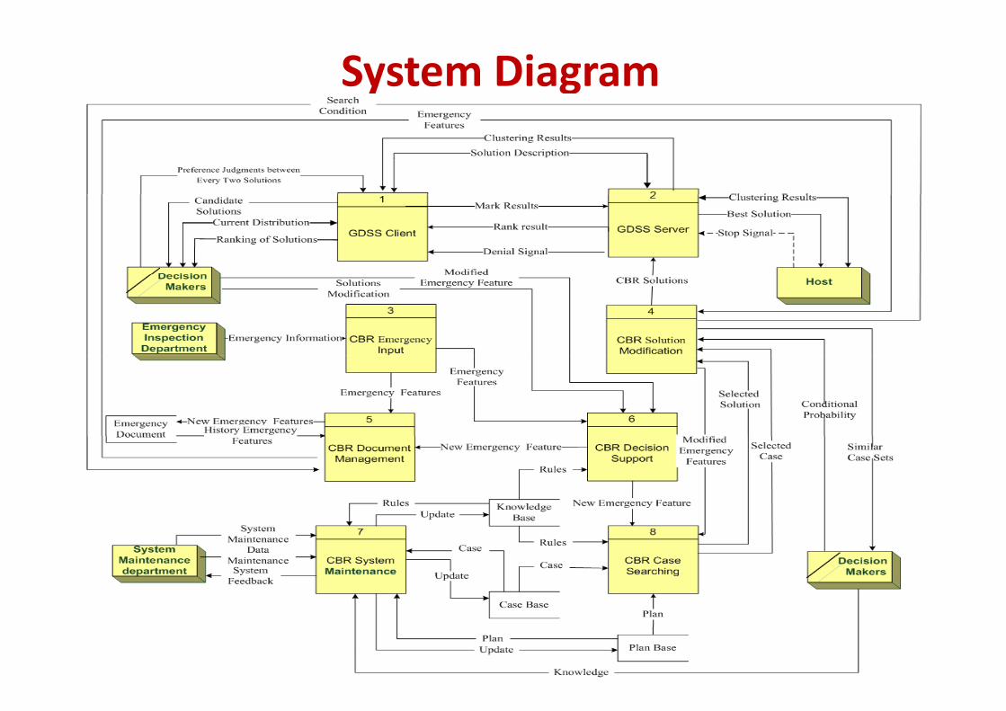
System Diagram
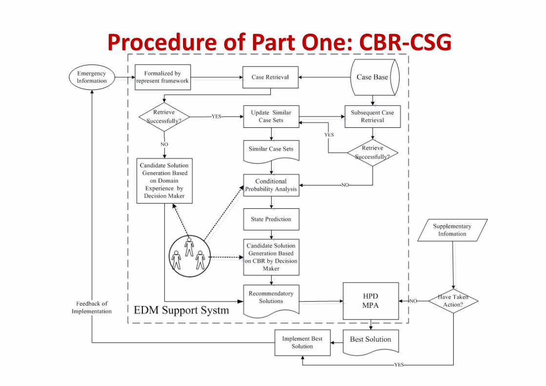
Procedure of Part One: CBR‐CSG
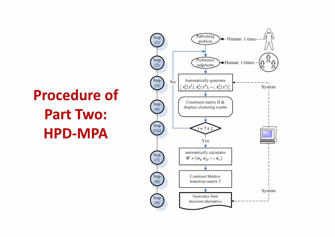
P d fProcedure of Part Two:Part Two: HPD‐MPA
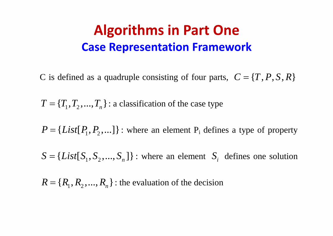
Algorithms in Part OneCase Representation Framework
C is defined as a quadruple consisting of four parts, { , , , }C T P S R=
1 2{ , ,..., }nT T T T= : a classification of the case type
1 2{ [ , ,...]}P List P P= : where an element Pi defines a type of property
1 2{ [ , ,..., ]}nS List S S S= : where an element iS defines one solution
1 2{ , ,..., }nR R R R= : the evaluation of the decision
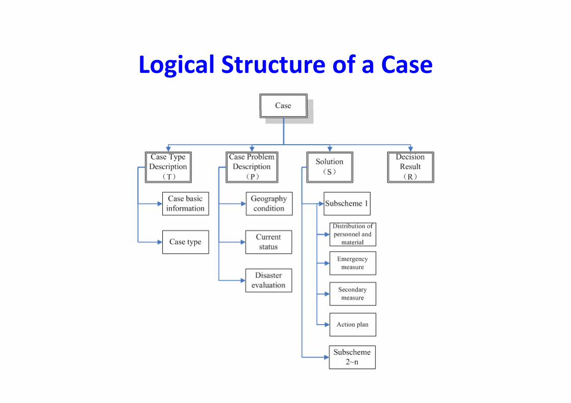
Logical Structure of a CaseLogical Structure of a Case
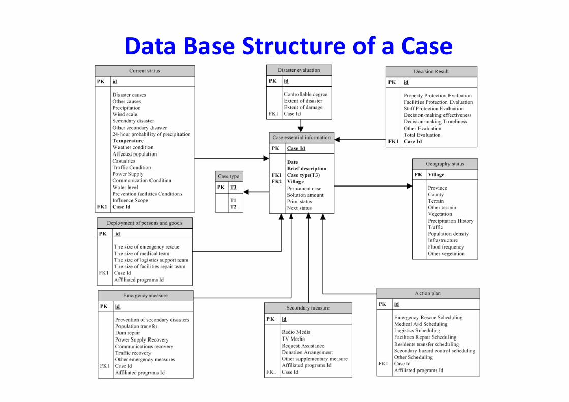
Data Base Structure of a Case
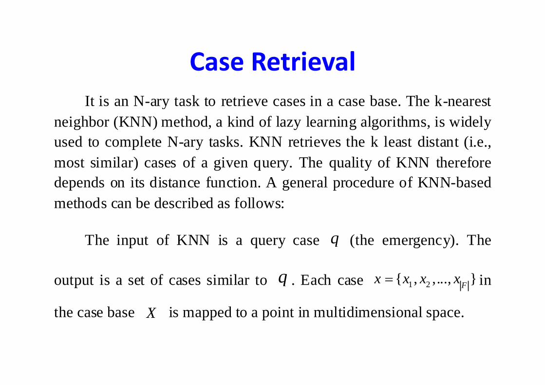
Case RetrievalCase RetrievalIt is an N-ary task to retrieve cases in a case base. The k-nearestIt is an N ary task to retrieve cases in a case base. The k nearest
neighbor (KNN) method, a kind of lazy learning algorithms, is widely used to complete N-ary tasks. KNN retrieves the k least distant (i.e.,p y ( ,most similar) cases of a given query. The quality of KNN therefore depends on its distance function. A general procedure of KNN-based methods can be described as follows:
Th i t f KNN i q (th ) ThThe input of KNN is a query case q (the emergency). The
output is a set of cases similar to q Each case { }x x x x= inoutput is a set of cases similar to q . Each case 1 2{ , ,..., }Fx x x x= in
the case base X is mapped to a point in multidimensional space.
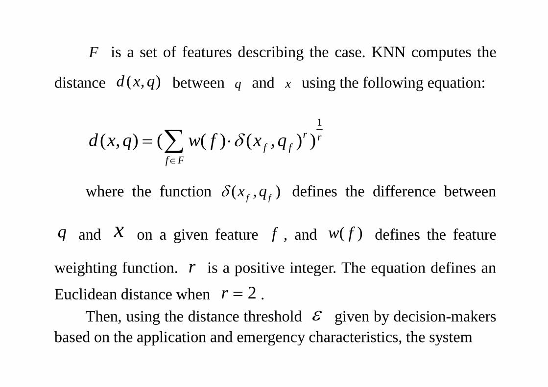
F is a set of features describing the case. KNN computes the
distance ( , )d x q between q and x using the following equation:
1
( , ) ( ( ) ( , ) )r rf fd x q w f x qδ= ⋅∑ ( ) ( ( ) ( ) )f f
f Fq f q
∈∑
where the function ( )x qδ defines the difference betweenwhere the function ( , )f fx qδ defines the difference between
q and x on a given feature f and ( )w f defines the featureq and on a given feature f , and ( )w f defines the feature
weighting function. r is a positive integer. The equation defines an
Euclidean distance when 2r = . Then, using the distance threshold ε given by decision-makers
based on the application and emergency characteristics, the system
retrieves all the cases whose distance to q are less than the given q g
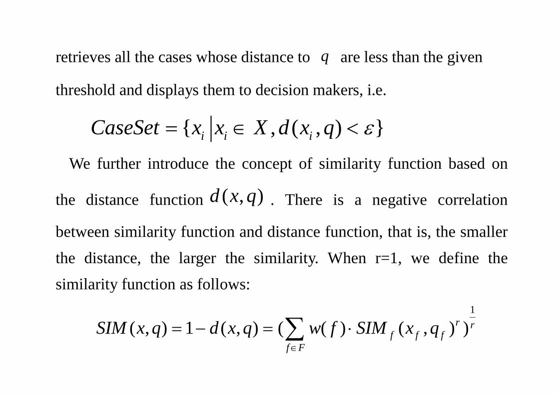
threshold and displays them to decision makers, i.e.
{ , ( , ) }i i iCaseSet x x X d x q ε= ∈ <
We further introduce the concept of similarity function based on
the distance f nction ( )d x q There is a negati e correlationthe distance function ( , )d x q . There is a negative correlation
between similarity function and distance function, that is, the smallerthe distance, the larger the similarity. When r=1, we define thesimilarity function as follows:similarity function as follows:
1
( , ) 1 ( , ) ( ( ) ( , ) )r rf f fSIM x q d x q w f SIM x q= − = ⋅∑
( , ) 1 ( , ) ( ( ) ( , ) )f f f
f F
SIM x q d x q w f SIM x q∈∑
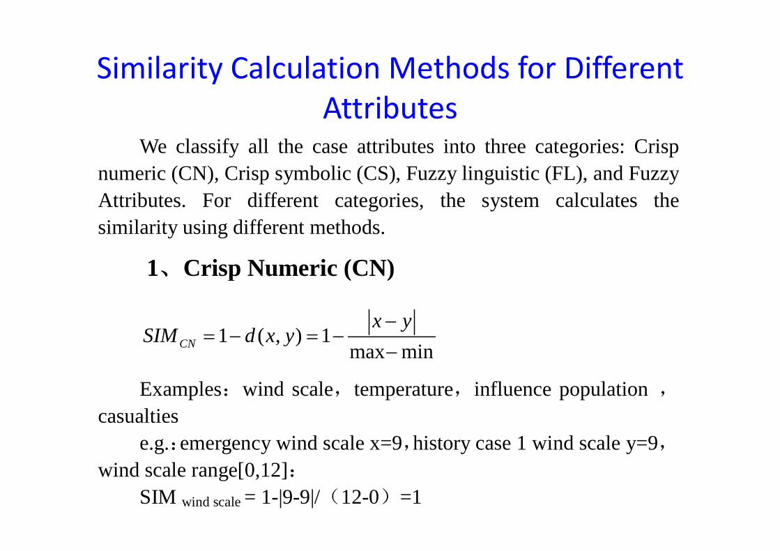
Similarity Calculation Methods for Different Attributes
We classify all the case attributes into three categories: CrispWe classify all the case attributes into three categories: Crisp numeric (CN), Crisp symbolic (CS), Fuzzy linguistic (FL), and FuzzyAttributes. For different categories, the system calculates the similarity using different methods.
1、Crisp Numeric (CN)1、Crisp Numeric (CN)
1 ( ) 1x y
SIM d x y−
= − = −1 ( , ) 1max minCNSIM d x y= =
− Examples:wind scale,temperature,influence population ,
casualties e.g.:emergency wind scale x=9,history case 1 wind scale y=9,
i d l [0 12]wind scale range[0,12]:SIM wind scale = 1-|9-9|/(12-0)=1
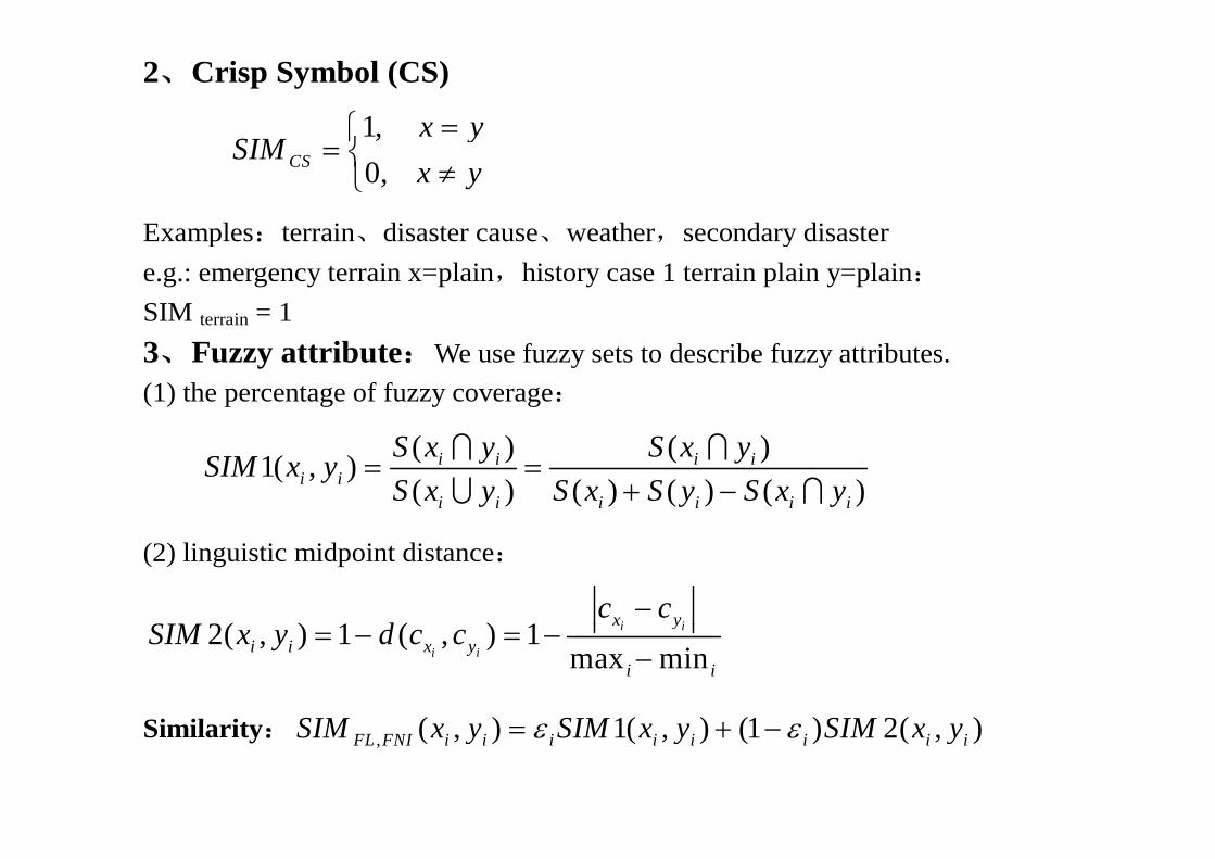
2、Crisp Symbol (CS)
1, x y=⎧⎨
,0, CS
ySIM
x y⎧
= ⎨ ≠⎩ Examples:terrain disaster cause weather secondary disasterExamples:terrain、disaster cause、weather,secondary disastere.g.: emergency terrain x=plain,history case 1 terrain plain y=plain: SIM terrain = 1 3、Fuzzy attribute:We use fuzzy sets to describe fuzzy attributes. (1) the percentage of fuzzy coverage:
( ) ( )1( , )( ) ( ) ( ) ( )
i i i ii i
i i i i i i
S x y S x ySIM x yS x y S x S y S x y
= =+ −
I I
U I
(2) linguistic midpoint distance:
2( ) 1 ( ) 1 i ix yc cSIM d
−2( , ) 1 ( , ) 1
max mini i
i i
x yi i x y
i i
SIM x y d c c= − = −−
Si il it ( ) 1( ) (1 ) 2( )SIM SIM SIMSimilarity: , ( , ) 1( , ) (1 ) 2( , )FL FNI i i i i i i i iSIM x y SIM x y SIM x yε ε= + −
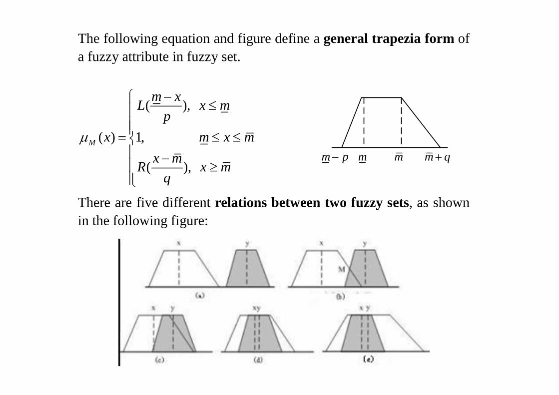
The following equation and figure define a general trapezia form of a fuzzy attribute in fuzzy set.y y
( )m xL x m−⎧ ≤⎪ ( ),
( ) 1, M
L x mp
x m x mμ
≤⎪⎪⎪= ≤ ≤⎨⎪
h fi diff i f h
m p m m m q− +( ), x mR x m
q
⎪ −⎪ ≥⎪⎩
There are five different relations between two fuzzy sets, as shown in the following figure:
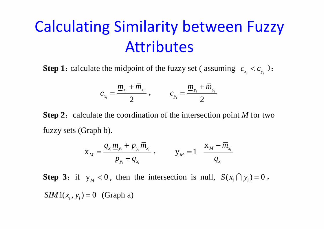
Calculating Similarity between Fuzzy Attributes
Step 1:calculate the midpoint of the fuzzy set ( assuming i ix yc c< ):
m m+ m m+2
i i
i
x xx
m mc
+= ,
2i i
i
y yy
m mc
+=
Step 2 calculate the coordination of the intersection point M for twoStep 2:calculate the coordination of the intersection point M for two
fuzzy sets (Graph b).
x i i i i
i i
x y y xM
y x
q m p mp q
+=
+,
xy 1 i
i
M xM
x
mq−
= −
Step 3:if y 0M < , then the intersection is null, ( ) 0i iS x y =I ,
1( ) 0SIM (G h )1( , ) 0i iSIM x y = (Graph a)
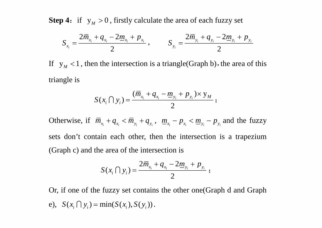
Step 4:if y 0M > , firstly calculate the area of each fuzzy set
2 2m q m p+ + 2 2m q m p+ +2 22
i i i i
i
x x x xx
m q m pS
+ − += ,
2 22
i i i i
i
y y y yy
m q m pS
+ − +=
If 1< th th i t ti i t i l (G h b) th f thiIf y 1M < , then the intersection is a triangle(Graph b),the area of this
triangle is
( ) y( )
2i i i ix x y y M
i i
m q m pS x y
+ − + ×=I ;
Otherwise, if i i i ix x y ym q m q+ < + ,
i i i ix x y ym p m p− < − and the fuzzy
sets don’t contain each other, then the intersection is a trapezium, p
(Graph c) and the area of the intersection is
2 2m q m p+ − +2 2( )
2i i i ix x y y
i i
m q m pS x y
+ +=I ;
Or if one of the fuzzy set contains the other one(Graph d and GraphOr, if one of the fuzzy set contains the other one(Graph d and Graph
e), ( ) min( ( ), ( ))i i i iS x y S x S y=I .
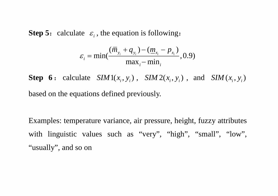
St 5 l l t th ti i f ll iStep 5:calculate iε , the equation is following:
( ) ( )i ( 0 9)i i i iy y x xm q m p+ − −( ) ( )
min( ,0.9)max min
i i i iy y x xi
i i
q pε =
−
St 6 l l t 1( )SIM 2( )SIM d ( )SIMStep 6: calculate 1( , )i iSIM x y , 2( , )i iSIM x y , and ( , )i iSIM x y
based on the equations defined previously.
Examples: temperature variance air pressure height fuzzy attributesExamples: temperature variance, air pressure, height, fuzzy attributes
with linguistic values such as “very”, “high”, “small”, “low”,
“usually”, and so on
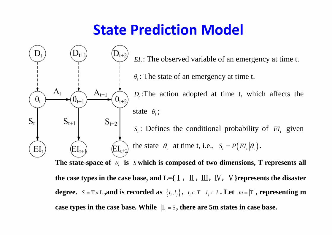
State Prediction Model
tEI : The observed variable of an emergency at time t.
tθ : The state of an emergency at time t.
h i d d i hi h ff htD :The action adopted at time t, which affects the
state tθ ;
tS : Defines the conditional probability of tEI given
th t t θ t ti t i ( )S P EI θthe state tθ at time t, i.e., ( )t t tS P EI θ= .
The state-space of tθ is S which is composed of two dimensions, T represents all
the case types in the case base, and L={Ⅰ,Ⅱ,Ⅲ,Ⅳ,Ⅴ}represents the disaster
degree. T LS = × ,and is recorded as { },i jt l , it T∈ jl L∈ . Let Tm = , representing m
case types in the case base. While L 5= , there are 5m states in case base.
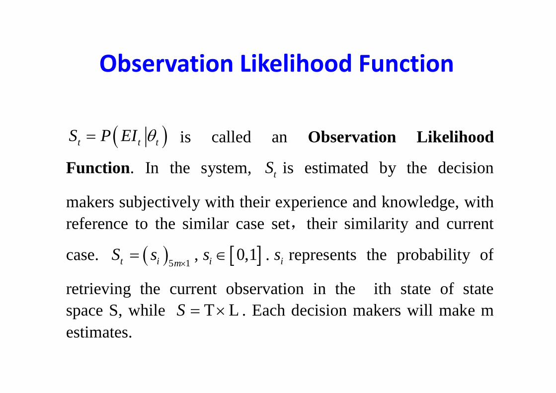
Observation Likelihood FunctionObservation Likelihood Function
is called an Observation Likelihood( )t t tS P EI θ=
Function. In the system, tS is estimated by the decision
k bj i l i h h i i d k l d i hmakers subjectively with their experience and knowledge, withreference to the similar case set,their similarity and current
case. ( )5 1t i mS s
×= , [ ]0,1is ∈ . is represents the probability of
t i i th t b ti i th ith t t f t tretrieving the current observation in the ith state of statespace S, while T LS = × . Each decision makers will make m estimatesestimates.
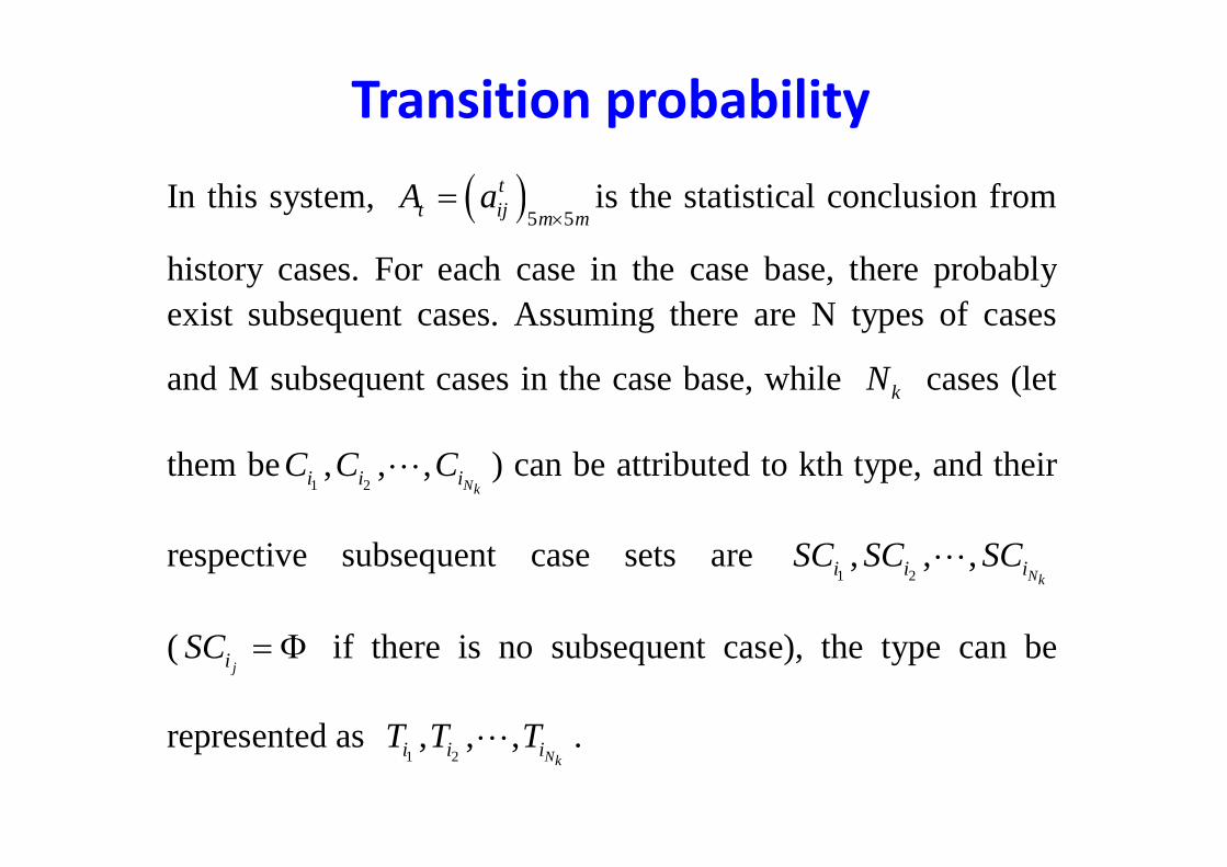
Transition probability
In this system, ( )5 5
tt ij m m
A a×
= is the statistical conclusion from
history cases. For each case in the case base, there probably exist subsequent cases. Assuming there are N types of cases
and M subsequent cases in the case base, while kN cases (let
them be1 2, , ,
Nki i iC C CL ) can be attributed to kth type, and their
respective subsequent case sets are 1 2, , ,
Nki i iSC SC SCL
(ji
SC = Φ if there is no subsequent case), the type can be
t d T T Trepresented as 1 2, , ,
Nki i iT T TL .
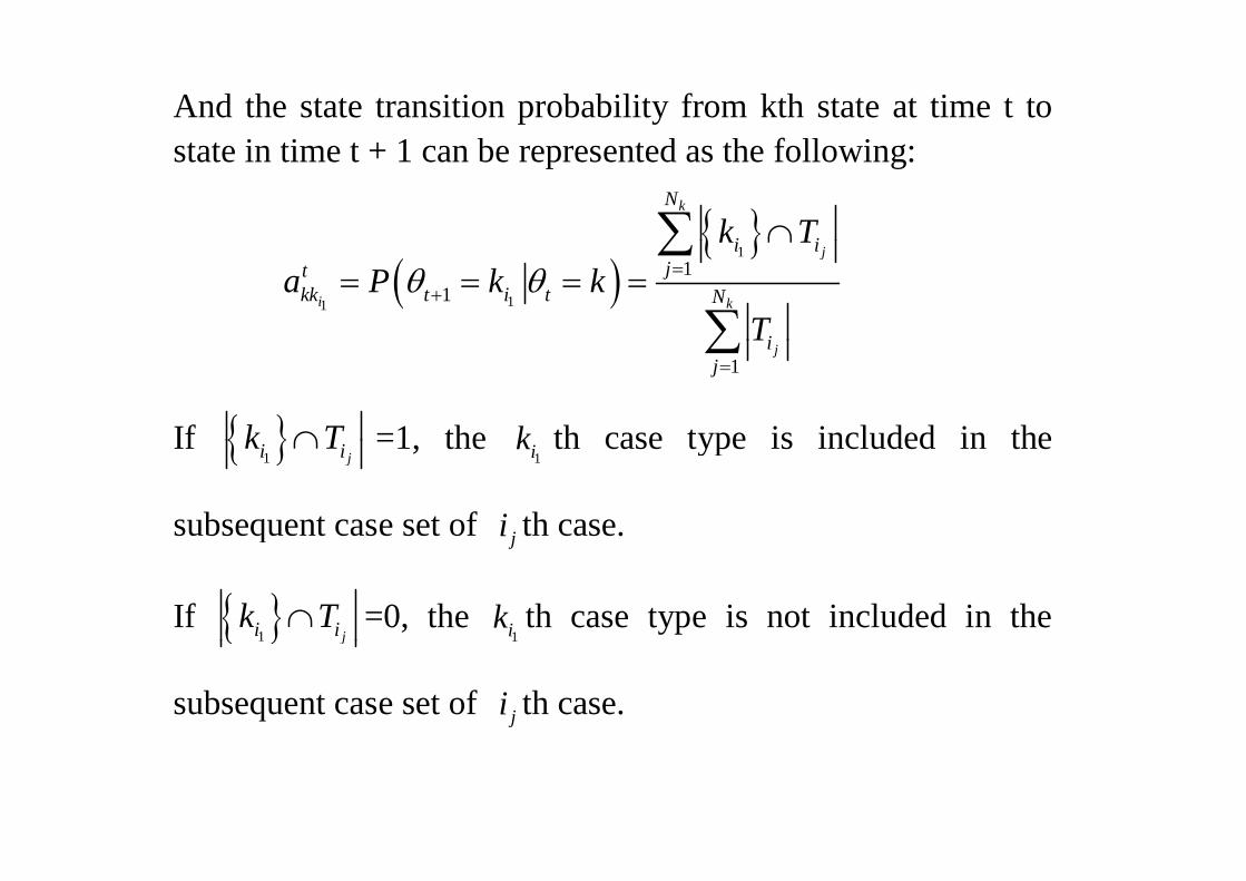
And the state transition probability from kth state at time t toi i 1 b d h f ll istate in time t + 1 can be represented as the following:
{ }kN
i ik T∩∑( )
{ }1
11
11
j
i k
i ijt
kk t i t N
i
k Ta P k k
Tθ θ =
+
∩= = = =
∑
∑
1ji
j=∑
If { }k T∩ =1 the k th case type is included in theIf { }1 ji ik T∩ =1, the 1i
k th case type is included in the
subsequent case set of ji th case.q j
If { }1 ji ik T∩ =0, the 1i
k th case type is not included in the { }1 j 1
subsequent case set of ji th case.
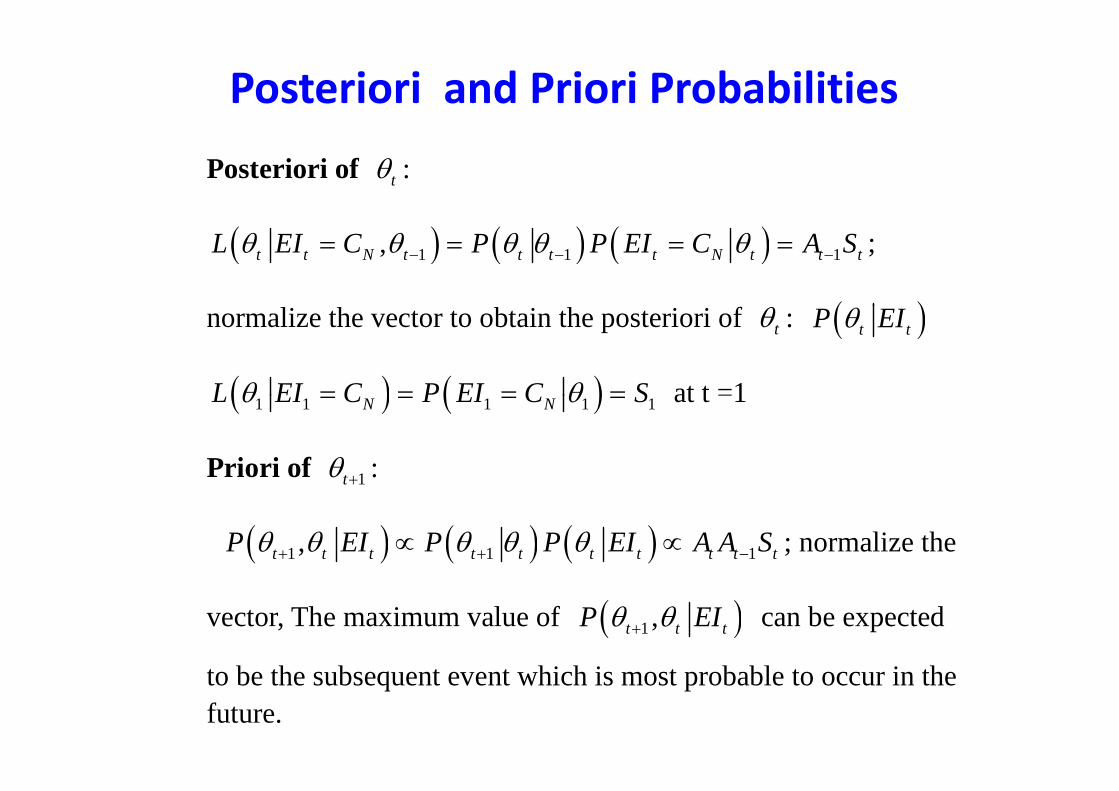
Posteriori and Priori Probabilities
Posteriori of tθ :
( ) ( ) ( )1 1 1,t t N t t t t N t t tL EI C P P EI C A Sθ θ θ θ θ− − −= = = = ;
( )normalize the vector to obtain the posteriori of tθ : ( )t tP EIθ
( ) ( )L EI C P EI C Sθ θ= = = = at t =1( ) ( )1 1 1 1 1N NL EI C P EI C Sθ θ= = = = at t 1
Priori of 1tθ + :
( ) ( ) ( )1 1 1,t t t t t t t t t tP EI P P EI A A Sθ θ θ θ θ+ + −∝ ∝ ; normalize the
vector, The maximum value of ( )1 ,t t tP EIθ θ+ can be expected
to be the subsequent event which is most probable to occur in the future.
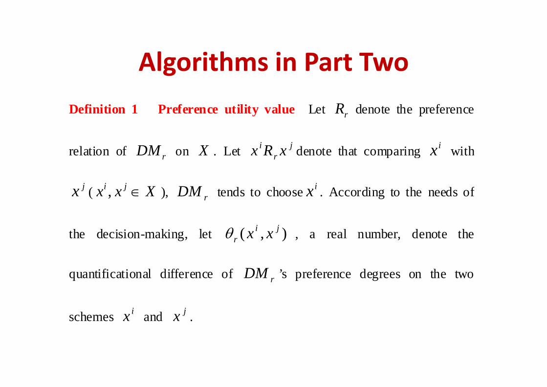
Algorithms in Part Two
D fi iti 1 P f tilit l L t R d t th f
Algorithms in Part Two
Definition 1 Preference utility value Let rR denote the preference
relation of DM on X Let ji xRx denote that comparing ix withrelation of rDM on X . Let jr xRx denote that comparing x with
jx ( i jx x X∈ ) DM tends to choose ix According to the needs ofx ( ,x x X∈ ), rDM tends to choose x . According to the needs of
the decision-making, let ),( ji xxθ , a real number, denote thethe decision making, let ),(r xxθ , a real number, denote the
quantificational difference of rDM ’s preference degrees on the two r
schemes ix and jx .
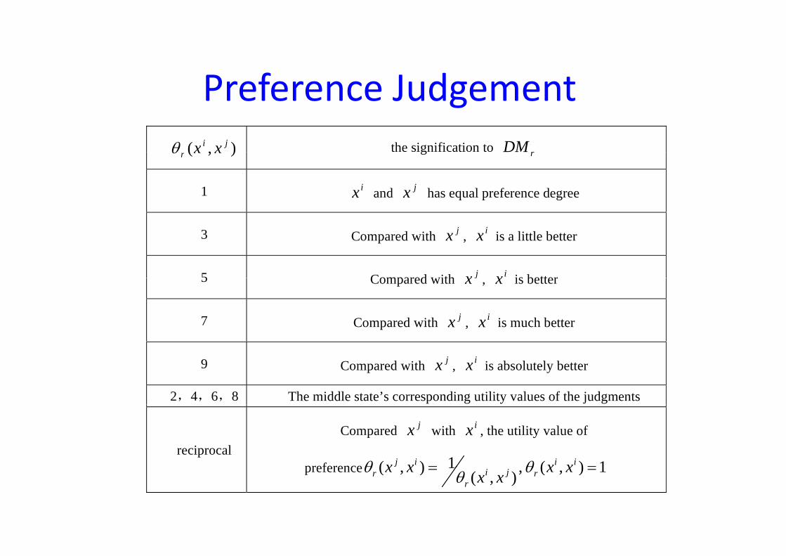
Preference Judgement),( ji xxθ the signification to DM
Preference Judgement),(r xxθ e s g c o o rDM
1 ix and jx has equal preference degree
3 Compared with jx , ix is a little better
5 Compared with jx ix is better5 Compared with jx , x is better
7 Compared with jx , ix is much better
9 Compared with jx , ix is absolutely better
2,4,6,8 The middle state’s corresponding utility values of the judgments
reciprocal Compared jx with ix , the utility value of
preference 1( ) ( ) 1j i i ix x x xθ θ= =preference 1( , ) , ( , ) 1( , )i jr rr
x x x xx xθ θθ= =
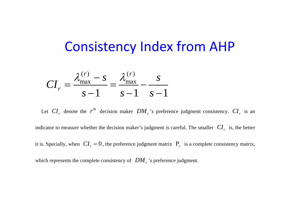
Consistency Index from AHP
( ) ( )r rs sλ λ−max max
1 1 1rs sCI
s s sλ λ−
= = −− − −
Let rCI denote the thr decision maker rDM ’s preference judgment consistency. rCI is an
indicator to measure whether the decision maker’s judgment is careful. The smaller rCI is, the better
it is. Specially, when 0rCI = , the preference judgment matrix rΡ is a complete consistency matrix, r r
which represents the complete consistency of rDM ’s preference judgment.
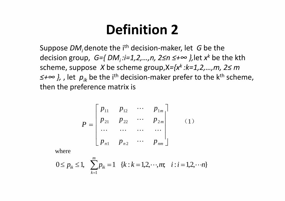
Definition 2Definition 2Suppose DMi denote the ith decision‐maker, let G be the d i i { i } l k b h k hdecision group, G={ DMi :i=1,2,…,n, 2≤n ≤+∞ },let xk be the kth scheme, suppose X be scheme group,X={xk :k=1,2,…,m, 2≤ m ≤+∞ } let p be the ith decision‐maker prefer to the kth scheme≤+∞ }, , let pik be the i decision‐maker prefer to the k scheme, then the preference matrix is
⎥⎥⎤
⎢⎢⎡
m
m
pppppp
PL
L
22221
11211
(1)
⎥⎥⎥
⎦⎢⎢⎢
⎣
=
nmnn ppp
P
L
LLLL
21
(1)
where },2,1:;,,2,1:{1,10 niimkkpp
m
ikik LL ===≤≤ ∑ 1k∑=
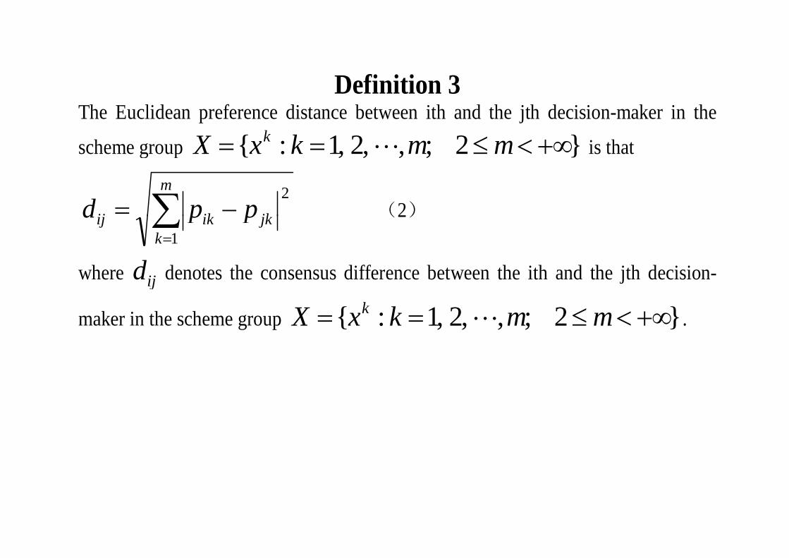
Definition 3Definition 3 The Euclidean preference distance between ith and the jth decision-maker in the
scheme group }2;,,2,1:{ +∞<≤== mmkxX k L is thatscheme group }2;,,2,1:{ +<≤mmkxX is that
∑ −=m
jkikij ppd2
(2)∑=k
jkikij ppd1
(2)
where ijd denotes the consensus difference between the ith and the jth decision-where ijd denotes the consensus difference between the ith and the jth decision
maker in the scheme group }2;,,2,1:{ +∞<≤== mmkxX k L .
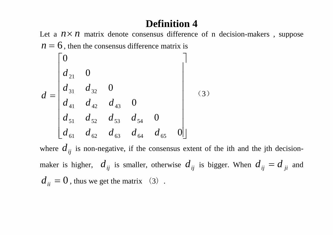
Definition 4 Let a nn× matrix denote consensus difference of n decision-makers , suppose , pp
6=n , then the consensus difference matrix is
⎥⎤
⎢⎡0
⎥⎥⎥⎥
⎢⎢⎢⎢
00
3231
21
ddd
( )
⎥⎥⎥
⎢⎢⎢=
00434241
3231
ddddddd
d (3)
⎥⎥⎥
⎦⎢⎢⎢
⎣ 00
6564636261
54535251
ddddddddd
dwhere ijd is non-negative, if the consensus extent of the ith and the jth decision-
maker is higher, ijd is smaller, otherwise ijd is bigger. When jiij dd = and j j jj
0=iid , thus we get the matrix (3).
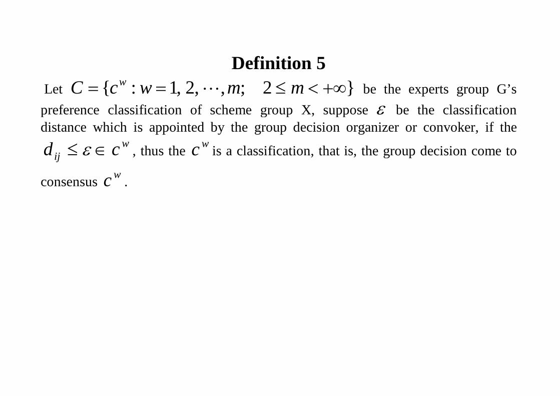
Definition 5Definition 5 Let }2;,,2,1:{ +∞<≤== mmwcC w L be the experts group G’s preference classification of scheme group X suppose ε be the classificationpreference classification of scheme group X, suppose ε be the classification distance which is appointed by the group decision organizer or convoker, if the
wij cd ∈≤ ε thus the wc is a classification that is the group decision come toij cd ∈≤ ε , thus the c is a classification, that is, the group decision come to
consensus wc .
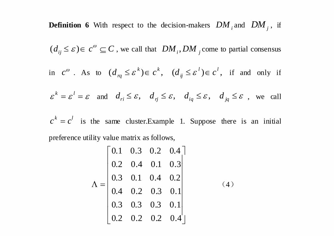
Definition 6 With respect to the decision-makers iDM and jDM , if
∈≤ )( εijd c Cω ⊆ , we call that ji DMDM , come to partial consensus
in cω . As to ,)(,)( llij
kkrq cdcd ∈≤∈≤ εε if and only if
lk εεε == lk and εεεε ≤≤≤≤ jqiqrjri dddd ,,, , we call
lk lk cc = is the same cluster.Example 1. Suppose there is an initial
preference utility value matrix as follows,
0.1 0.3 0.2 0.40.2 0.4 0.1 0.3⎡ ⎤⎢ ⎥⎢ ⎥
0.3 0.1 0.4 0.20.4 0.2 0.3 0.1
⎢ ⎥⎢ ⎥
Λ = ⎢ ⎥⎢ ⎥⎢ ⎥
(4)
0.3 0.3 0.3 0.10.2 0.2 0.2 0.4
⎢ ⎥⎢ ⎥⎣ ⎦
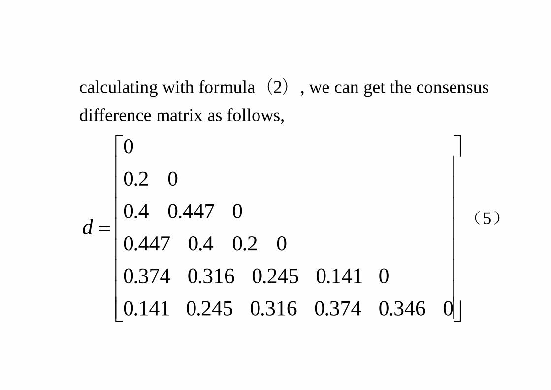
calculating with formula(2), we can get the consensus difference matrix as follows,
⎤⎡0
⎥⎥⎤
⎢⎢⎡
02.00
⎥⎥⎥⎥
⎢⎢⎢⎢
=020404470
0447.04.0d (5)
⎥⎥⎥⎥
⎢⎢⎢⎢
0141.0245.0316.0374.002.04.0447.0
⎥⎥⎦⎢
⎢⎣ 0346.0374.0316.0245.0141.0
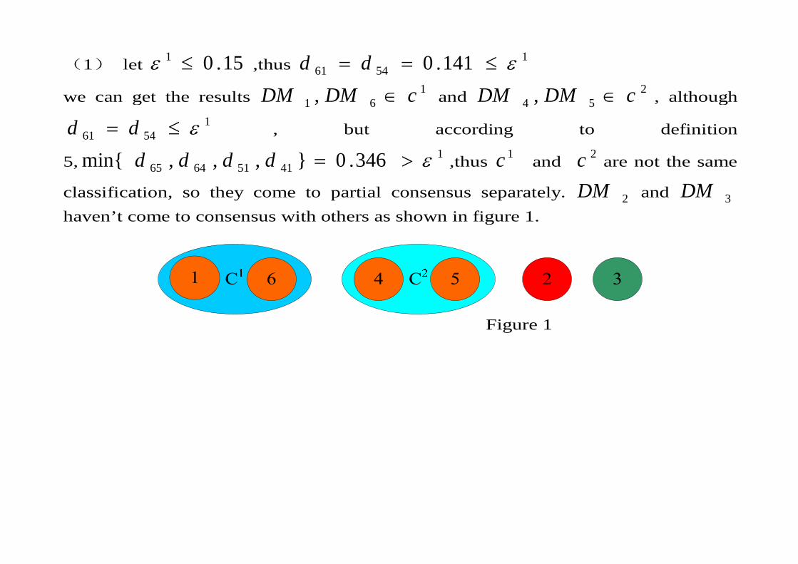
(1) let 15.01 ≤ε ,thus 15461 141.0 ε≤== dd
1DMDM 2DMDMwe can get the results 161 , cDMDM ∈ and 2
54 , cDMDM ∈ , although 1
5461 ε≤= dd , but according to definition 13460}i { dddd 1 25, 1
41516465 346.0},,,min{ ε>=dddd ,thus 1c and 2c are not the same
classification, so they come to partial consensus separately. 2DM and 3DMhaven’t come to consensus with others as shown in figure 1haven t come to consensus with others as shown in figure 1.
Figure 1
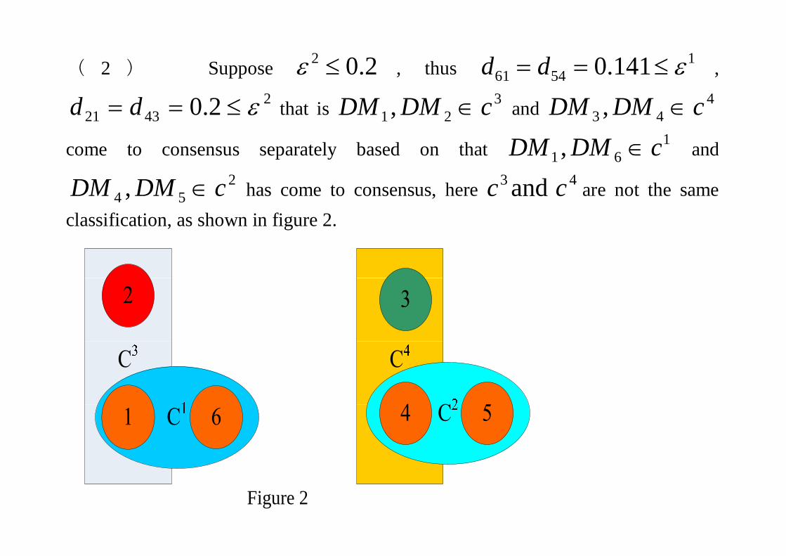
( 2 ) Suppose 2.02 ≤ε , thus 15461 141.0 ε≤== dd ,
24321 2.0 ε≤== dd that is 3
21 , cDMDM ∈ and 443 , cDMDM ∈
come to consensus separately based on that 161 cDMDM ∈ andcome to consensus separately based on that 61 , cDMDM ∈ and
254 , cDMDM ∈ has come to consensus, here 43 and cc are not the same
l ifi ti h i fi 2classification, as shown in figure 2.
Figure 2
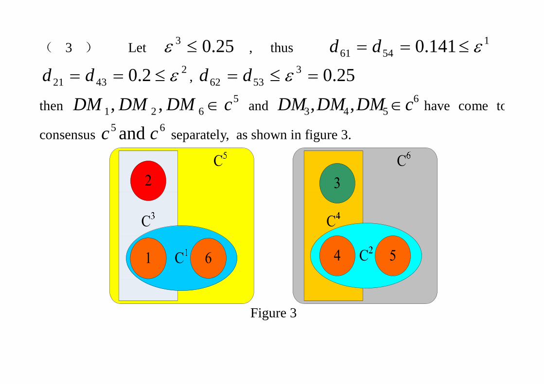
( 3 ) Let 25.03 ≤ε , thus 15461 141.0 ε≤== dd ,
24321 2.0 ε≤== dd , 25.03
5362 =≤= εdd
then 5cDMDMDM ∈ and 6cDMDMDM ∈ have come tothen 621 ,, cDMDMDM ∈ and 543 ,, cDMDMDM ∈ have come to
consensus 65 and cc separately, as shown in figure 3.
Figure 3
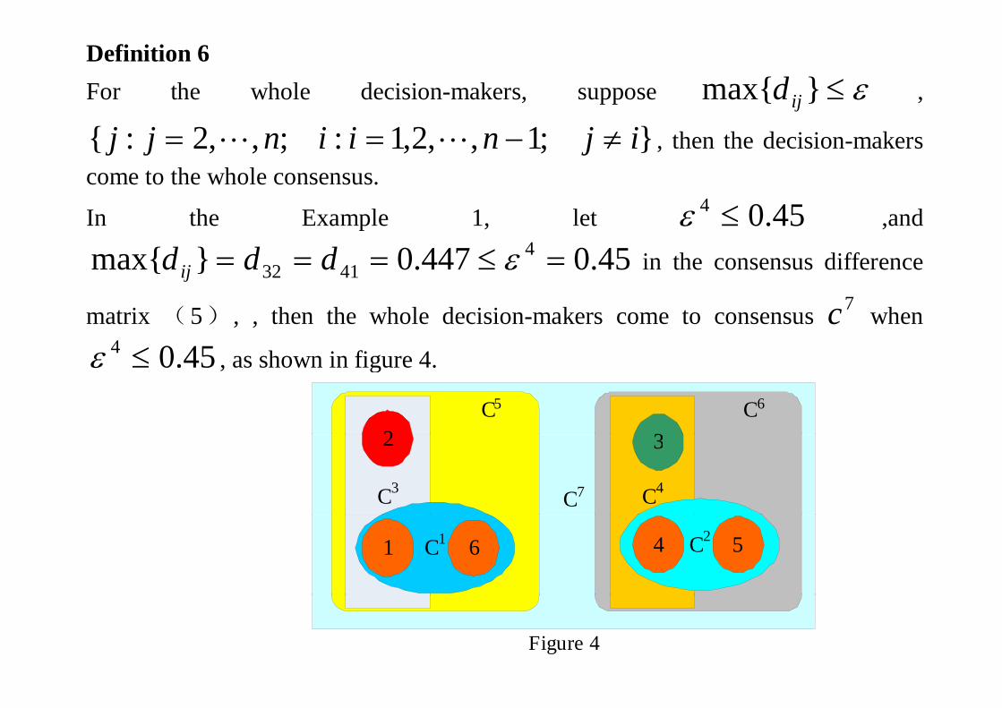
Definition 6 For the whole decision-makers, suppose ε≤}max{ ijd ,
};1,,2,1:;,,2:{ ijniinjj ≠−== LL , then the decision-makers come to the whole consensus.
In the Example 1, let 45.04 ≤ε ,and
45.0447.0}max{ 44132 =≤=== εdddij in the consensus difference}{ 4132ij
matrix (5) , , then the whole decision-makers come to consensus 7c when
4504 ≤ε h i fi 445.0≤ε , as shown in figure 4.
C6 C5
32
C7 C4C3
32
C1 C24 561
Figure 4
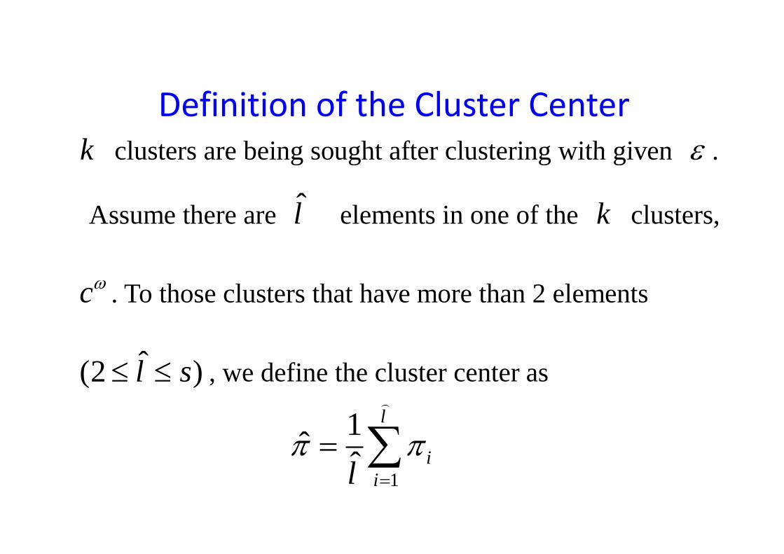
Definition of the Cluster Centerk clusters are being sought after clustering with given εk clusters are being sought after clustering with given ε .
Assume there are l̂ elements in one of the k clusters Assume there are l elements in one of the k clusters,
cω . To those clusters that have more than 2 elements
ˆ(2 )l s≤ ≤ , we define the cluster center as
1ˆ ˆl
ilπ π= ∑
)
1il =∑
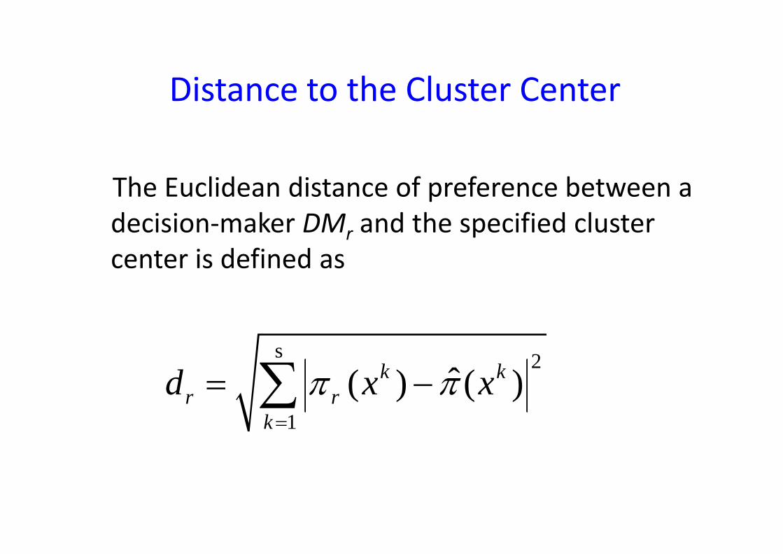
Distance to the Cluster CenterDistance to the Cluster Center
The Euclidean distance of preference between a d i i k DM d h ifi d ldecision‐maker DMr and the specified cluster center is defined as
s 2ˆ( ) ( )k k
r rd x xπ π= −∑1
r rk=∑
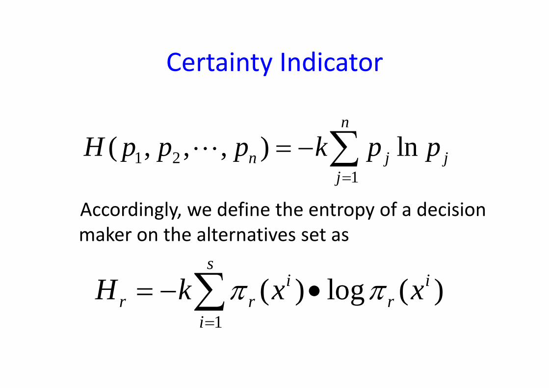
Certainty IndicatorCertainty Indicator
( ) ln
n
H p p p k p p= − ∑L1 21
( , , , ) lnn j jj
H p p p k p p=
= ∑L
Accordingly, we define the entropy of a decision maker on the alternatives set asmaker on the alternatives set as
( ) l ( )s
i iH k∑1
( ) log ( )i ir r r
iH k x xπ π
=
= − •∑1i
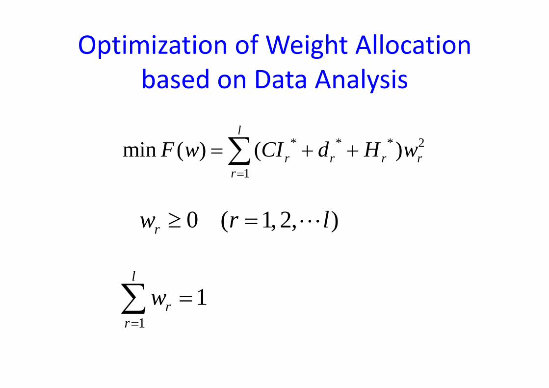
Optimization of Weight Allocation based on Data Analysis
* * * 2min ( ) ( )l
F w CI d H w= + +∑1
min ( ) ( )r r r rr
F w CI d H w=
= + +∑
0 ( 1, 2, )rw r l≥ = L
l
11r
rw
=
=∑ 1r
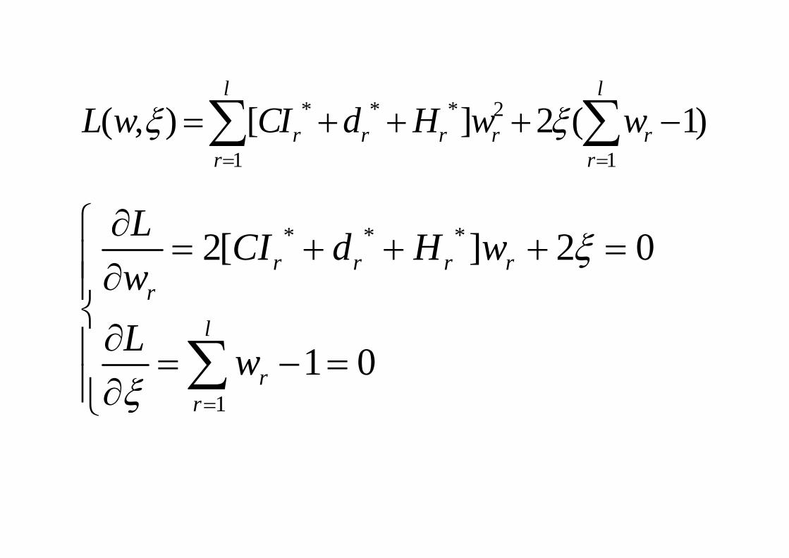
l l * * * 2( , ) [ ] 2 ( 1)l l
r r r r rL w CI d H w wξ ξ= + + + −∑ ∑1 1r r= =
L∂⎧ * * *2[ ] 2 0r r r rL CI d H ww
ξ∂⎧ = + + + =⎪∂⎪ rl
wL∂⎪
⎨∂⎪ ∑
11 0r
r
L wξ =
∂⎪ = − =⎪∂⎩
∑1rξ =⎩
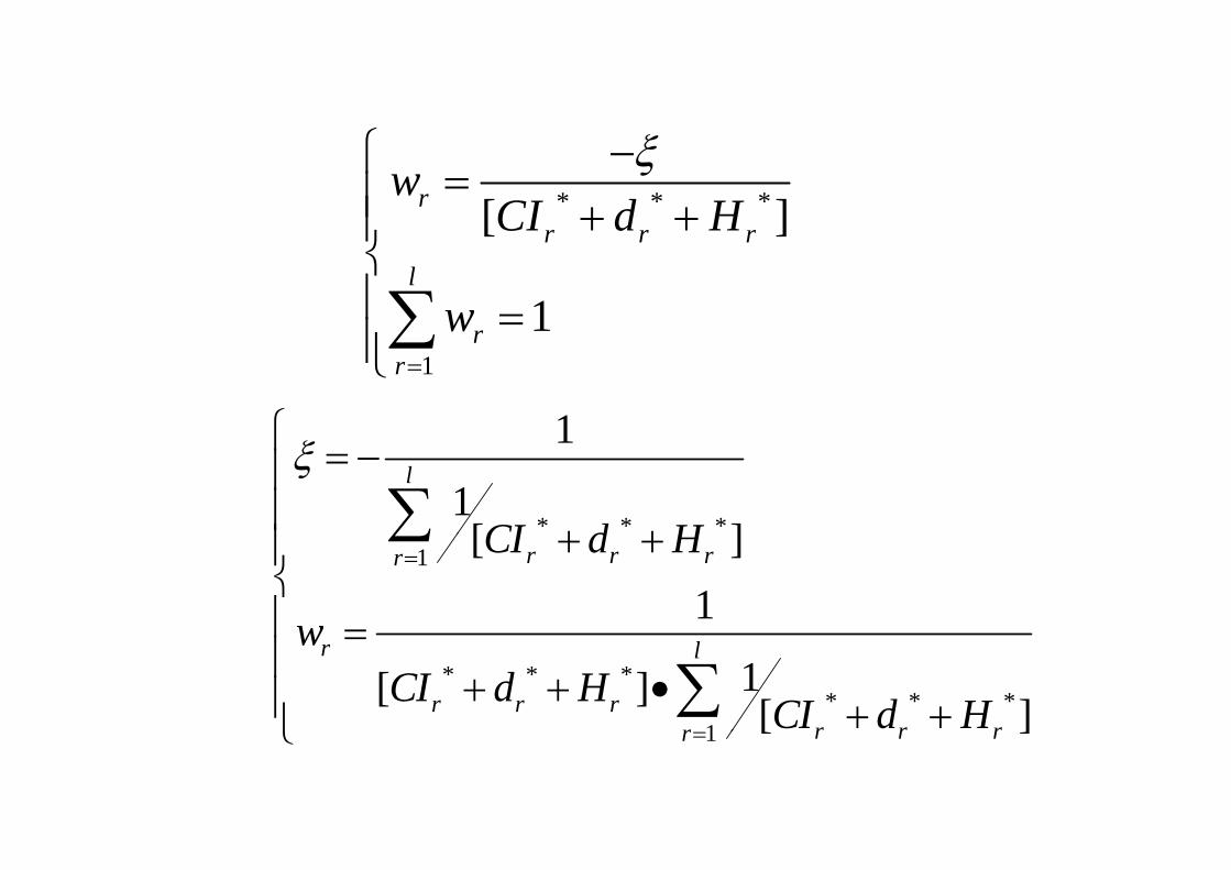
ξ⎧ * * *[ ]r
r r r
wCI d H
ξ−⎧ =⎪ + +⎪⎨
[ ]
1
r r rl
rw
⎪⎨⎪ =⎪⎩∑
1r
r=⎪⎩∑
1⎧
* * *
1
1[ ]
l
CI d H
ξ⎧ = −⎪⎪ + +⎪
∑1 [ ]
1r r rr CI d H
w
= + +⎪⎨⎪ =
∑
* * ** * *
1
1[ ] [ ]
r l
r r rr r rr
wCI d H CI d H
⎪ =⎪
+ + •⎪ + +⎩∑
1 [ ]r r rr=⎩
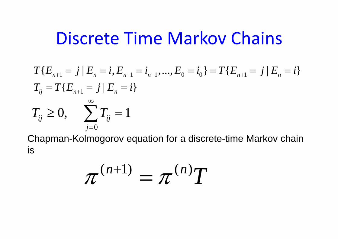
Discrete Time Markov ChainsDiscrete Time Markov Chains
1 1 1 0 0 1
1
{ | , ,..., } { | }{ | }
n n n n n n
ij n n
T E j E i E i E i T E j E iT T E j E i
+ − − +
+
= = = = = = == = =1{ | }ij n nj+
0, 1ij ijT T
∞
≥ =∑0
ij ijj=∑
Chapman-Kolmogorov equation for a discrete-time Markov chain iis
( 1) ( )n n Tπ π+ ( ) ( )Tπ π=
Hidden Pattern of Group Preference Change Based on Markov Chain
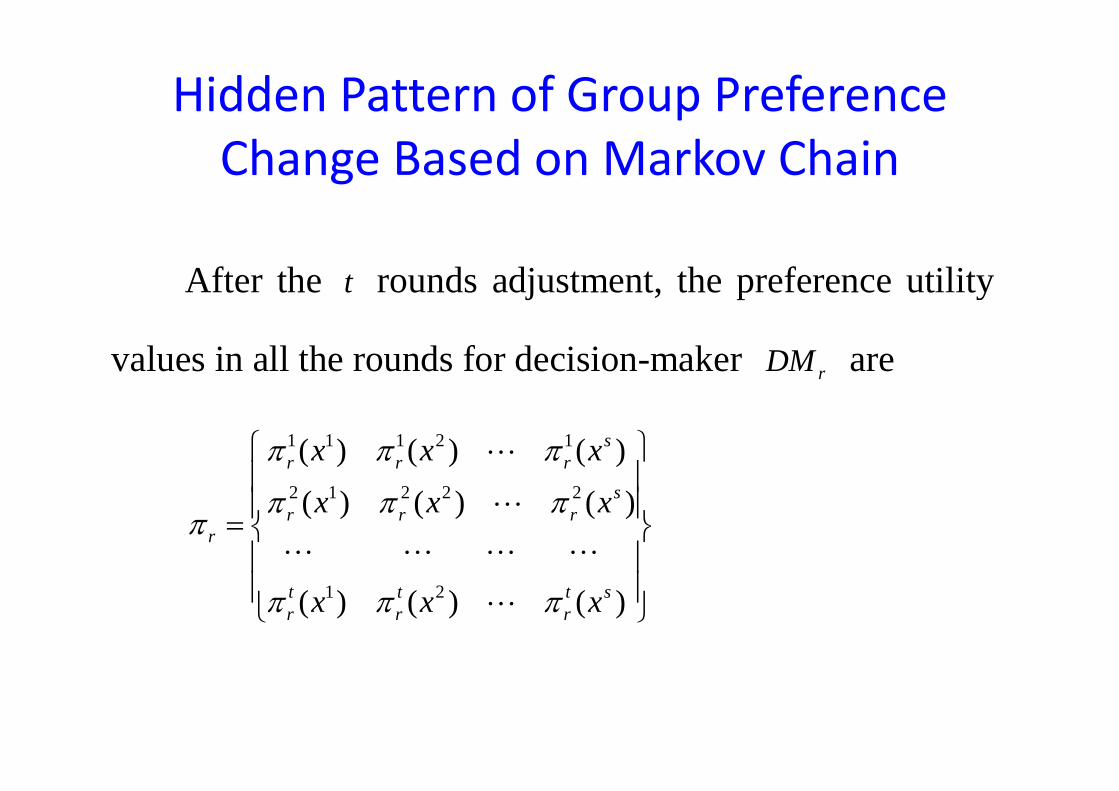
After the t rounds adjustment, the preference utility
values in all the rounds for decision-maker rDM are
1 1 1 2 1( ) ( ) ( )sr r rx x xπ π π⎧ ⎫
⎪ ⎪L
2 1 2 2 2( ) ( ) ( )sr r r
rx x xπ π π
π⎪ ⎪⎪ ⎪= ⎨ ⎬⎪ ⎪⎪ ⎪
L
L L L L
1 2( ) ( ) ( )t t t sr r rx x xπ π π⎪ ⎪
⎩ ⎭L
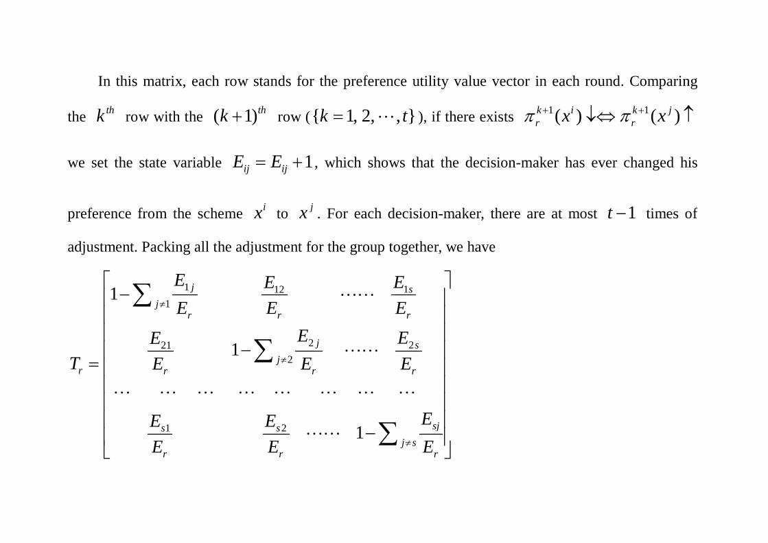
In this matrix, each row stands for the preference utility value vector in each round. Comparing, p y p g
the thk row with the ( 1)thk + row ({ 1, 2, , }k t= L ), if there exists 1 1( ) ( )k i k jr rx xπ π+ +↓⇔ ↑
we set the state variable 1ij ijE E= + , which shows that the decision-maker has ever changed his
f f th h i t j F h d i i k th t t 1t ti fpreference from the scheme ix to jx . For each decision-maker, there are at most 1t − times of
adjustment. Packing all the adjustment for the group together, we have
⎡ ⎤1 1121
1 j sj
r r r
E EEE E E
E EE
≠
⎡ ⎤−⎢ ⎥
⎢ ⎥⎢ ⎥
∑ LL
2 2212
1 j sj
r r r r
E EET E E E≠
⎢ ⎥−⎢ ⎥
= ⎢ ⎥⎢ ⎥⎢ ⎥
∑ LL
L L L L L L L L
1 2 1 sjs sj s
r r r
EE EE E E≠
⎢ ⎥⎢ ⎥
−⎢ ⎥⎣ ⎦
∑LLr r r⎣ ⎦
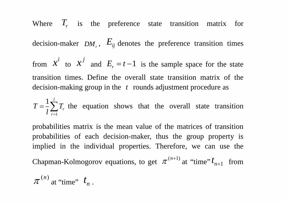
Where rT is the preference state transition matrix for
decision-maker rDM , ijE denotes the preference transition times
from ix to
jx and 1rE t= − is the sample space for the state
transition times Define the overall state transition matrix of thetransition times. Define the overall state transition matrix of thedecision-making group in the t rounds adjustment procedure as
1 l
1
1r
rT T
l =
= ∑ the equation shows that the overall state transition
b biliti t i i th l f th t i f t itiprobabilities matrix is the mean value of the matrices of transitionprobabilities of each decision-maker, thus the group property isimplied in the individual properties Therefore we can use theimplied in the individual properties. Therefore, we can use the
Chapman-Kolmogorov equations, to get ( 1)nπ + at “time” 1nt + from
( )nπ at “time” nt .
Conclusions 1) From the Battle of Midway, we find a lot of
commonalities in Emergencies and some Common problemscan be supported by information systems. Informationsystems could improve emergency response in applying Case‐Based Reasoning, finishing rapid calculations and quickforecast, reducing response time and speeding up consensusb ildibuilding.
2) In emergencies, human decision makers often draw anl b t th i ti d hi t i l d tanalogy between the existing emergency and historical data
and then make a history‐based decision. However, it isdifficult and sometimes even impossible for most decisiondifficult and sometimes even impossible for most decisionmakers to grasp the specifics of historical events in order tomake an analogy and apply it to a specific emergency inmake an analogy and apply it to a specific emergency inlimited time, therefore, cases‐based GDSS is useful.
3) B d hi t i l l i th t t ti ll3) Based on historical analogies, the system automaticallyfinds the transition probabilities of events from one state toanother Such information helps decision makers analyze andanother. Such information helps decision makers analyze andevaluate the differences between current emergency andhistorical analogies. Integrating transition probabilities andg g g pdomain expertise of decision makers, the system predicts thenext possible state and help decision makers put forward a
t did t l ticorrect candidate solution.
4) We finished the analysis design and most of the4) We finished the analysis, design and most of theimplementation of the cases-based GDSS. A Flood casesbase have be constructed, including about one hundredgprevious events. We are now conducting an experiment atChina Executive Leadership Academy-Pudong.
5) Our current GDSS mainly supportsnumerical computation In near future wenumerical computation. In near future, weplan to formalize the emergency
i f k i d i irepresentation framework using descriptionlogics and semantic web related technology inorder to further support logic reasoning.

Th k YThank You
Supplementary slidesSupplementary slides
• Example of CBR‐CSG
• Example of HPD‐MPAp