Embed Size (px)
Citation preview
8 September 2016 DRAFT: NOT FOR CITATION
1 | P a g e
The Fiscal Policy Space of Cities:
A Comprehensive Framework for City Fiscal Decision-Making
Report prepared by the Fiscal Policy Space of Cities research team
at the University of Illinois at Chicago1
Abstract
This paper describes a new framework—the Fiscal Policy Space (FPS)—for assessing the unique
financial, economic, and political parameters cities operate under. We devised the FPS framework to help
model how city leaders confront revenue and spending decisions and the environment that constrains their
decision-making space. The FPS framework includes three attributes that shape policy choices: 1) the
intergovernmental system, 2) the underlying economic and fiscal system, and 3) citizen demands for
services and the local political culture. We created new measures from 100 cities’ experiences to depict
how the interaction of the three dimensions constrains a city’s FPS and shapes its ability to respond to
economic shifts. We find, for example, that cities with the most constrained FPS are more likely to spend
more per capita and, during the Great Recession, drew down reserves dramatically; and those with the
least constrained FPS spent less per capita and maintained their reserves during the Great Recession. The
FPS is a construct that reshapes the narrative about cities and their fiscal behavior. As cities continue to
emerge from the Great Recession, the FPS offers insight on where to focus policy and guidance from
federal, state, and local policymakers within the complex intergovernmental system.
The generous support of the John D. and Catherine T. MacArthur Foundation is greatly appreciated. We
would like to thank Valerie Chang for her unwavering commitment to this research project that focuses
on the municipal finances and fiscal policy behavior of American cities.

8 September 2016 DRAFT: NOT FOR CITATION
2 | P a g e
Overview
Cities and metropolitan regions are the drivers of economic wealth and competitiveness.2
Underlying cities’ abilities to create and sustain economic growth is the fiscal capacity of
general‐purpose municipal governments. These governments invest in local economies;
construct, maintain, and operate the infrastructure on which economic development is built; and
ensure the health, safety, and welfare of the people in their communities.3 The consequences of
the Great Recession have been severe for cities and their economic regions. Underlying
economic conditions have compromised the capacity of cities to invest in future economic
growth. These conditions have undermined the fiscal capacity of city governments to raise
adequate resources and adequately fund investment and services.
A city’s fiscal capacity to extract resources or revenue to fund basic services and infrastructure is
unique. Some, but not all, cities can tax income and utilities. Some can tax real estate transfers
and tangible property. Others can tax retail sales and motor fuels. Still others can tax gross
receipts. Cities, like all organizations, share similarities, but like all organizations, it is their
differences that define them.
The national debate on cities—their precarious fiscal positions during and after the recession,
and how to prevent another Detroit—is not much different from the national debate on health
care. Everyone has a favorite treatment (policy) and every city claims it won’t work in their city.
In one respect, the refrain that “it won’t work here” is understandable. After all, cities, much like
human beings, evolve and adapt to changing economic, social, and political circumstances. With
time, new personalities, different community needs and wants, and new identities emerge,
making cities that at one time might have shared similar characteristics appear quite different
over time.
The main theme of the Fiscal Policy Space framework is analogous to the personalized or
precision medicine initiative underway. After all, wrote President Obama in the 2016 budget
address, “Treatments that are very successful for some patients don't work for others. Think
about it, if you need glasses, you aren't assigned a generic pair. You get a prescription
customized for you.”4
Cities, too, are idiosyncratic. The effects of policy prescriptions are unpredictable, and each
city’s unique history, demographic makeup, land use and development patterns, and more
require us to consider each city individually. That is what the Fiscal Policy Space begins to do.
8 September 2016 DRAFT: NOT FOR CITATION
3 | P a g e
The Economic and Fiscal Condition of U.S. Cities
The economic malaise following the recession of 2008-09 has lingered longer than any other
since the Great Depression, and the “fiscal recession” has lingered longer still.5
Although local governments, especially those that rely on the property tax, were not affected as
quickly as their state and federal counterparts, cities in general experienced declining general
fund revenue for six consecutive years starting in 2007.6 In constant dollars, the average city lost
between 0.9 percent and 4.5 percent of its revenue from the previous year for five consecutive
years between 2007 and 2012.
Nonetheless, the “average” city masks the variation in city fiscal positions. City revenue
structures are too complex for broad-stroke analyses. There is no average or typical municipal
revenue structure. In the twentieth century, cities’ own-source revenues shifted from a near total
reliance on the property tax to a complex mix. Today, cities’ property tax revenues compose only
a slightly greater share than their combined sales and income tax revenues, which are also nearly
equal to city user charge revenues.7 In fact, approximately 9 percent of U.S. municipalities have
the authority to levy an income tax, and 55 percent have authority to levy a sales tax.
The contemporary revenue picture represents the direct fallout from the Great Recession, and it
has dramatic implications for the services that cities provide and the quality of life of the
residents and communities. The annual fiscal surveys conducted by the National League of Cities
in cooperation with the University of Illinois at Chicago show a persistent trend of service cuts
and retrenchment. The two areas most likely to be cut during the Great Recession were personnel
(wages, pensions, and other benefits) and infrastructure projects―cuts that, ironically, provide a
drag on the national economic recovery.8 The unemployment numbers from the U.S. Bureau of
Labor Statistics reveal that approximately a half million jobs were lost in the local government
sector during the Great Recession.9 At the same time, cities have also made severe cuts in a
range of services, from social and human services, to parks and recreation and public safety.
Identifying solutions and pathways requires an enhanced understanding of the underlying fiscal
and economic capacities of cities and the factors that drive those capacities. Unfortunately, the
national dialogue about the governance of cities and regions is poorly informed about the range
of variation in local governance and economic models, and it lacks timely, relevant data
describing current and ongoing conditions. Assessments of local conditions too often assume
similarities in revenue and governance structures, ignore wide variation in underlying economic
drivers, and lack understanding of the myriad differences in local political culture, traditions, and
institutions.

8 September 2016 DRAFT: NOT FOR CITATION
4 | P a g e
The Frame: Fiscal Policy Space of Cities
Much of the research and policy discourse has focused on understanding the changing dynamics
of the economy. Some has focused on the role of state governments, but much less has focused
on the economic and fiscal dynamics of cities.10
The size and shape of the fiscal policy space of
cities vary considerably. Cities are authorized or required by state governments to perform
certain responsibilities and to raise certain kinds of revenue. They may also offer other, elective
services in response to local demands and political culture and may often generate revenue from
these nonprescribed activities. Underlying economic and demographic factors also drive city
fiscal capacity. The variation in fiscal policy space suggests that there are at least 50 municipal
systems framed by each state’s constitutional structures. Yet, even within states, cities’ revenue
systems are not homogeneous. Although each municipality is unique, it is also true that patterns
and typologies of resource‐generating activities and institutions can be identified that can better
inform our understanding of fiscal and economic decision‐making, adaptation, and governance.
The Fiscal Policy Space (FPS) framework contends that policymakers operate within a confined
decision-making environment. This confined environment typically transcends periods of change
in the business cycle, defining the range of options available to local policymakers in periods of
economic growth and decline. The key attributes of this decision environment, which are adapted
from earlier work by Pagano and Hoene,11
collectively mold the “space” within which fiscal
policy is addressed. They include the following:
The intergovernmental context, including both state-imposed and locally imposed
limitations on taxes and expenditures.
The fiscal base, meaning the link between a city’s economic base and its fiscal
architecture or authority to tap into a city’s underlying economy.
The demands and preferences of citizens for a quantity and quality of services and the
local political culture that creates a set of expectations, norms of conduct and behavior,
and informal rules.
Sample Cities
We collected data for the FPS project from 100 cities that are representative of the municipal
sector, provided variation in terms of revenue structures and region of the country, and had
available data.12
A key challenge in selecting a sample of cities that is economically representative of the
municipal sector is that economic output data are not collected regularly for a wide range of
cities. For example, gross domestic product estimates are typically available for metropolitan
areas but not as readily or regularly available for individual cities. As a result, the project team

8 September 2016 DRAFT: NOT FOR CITATION
5 | P a g e
used a selection method that attempts to crudely approximate the relative economic and fiscal
importance of large cities within metropolitan areas. We selected project cities on the basis of
their relative population size and the relative population size of their metropolitan statistical area
(MSA), based on the 2011 census estimates. To be included in the sample, a city must be among
the largest U.S. central cities and be within the largest MSA’s in the United States. For example,
a smaller central city located in a large MSA would not be included in the sample, or a larger
central city located in a smaller MSA would not be included. The interaction of city size and
MSA size produced a list of cities that approximates the most economically and fiscally
influential cities in the United States.
We have created a public-access data portal that includes more than 600 variables for the time
period 1992-2012 for the 100 sample cities at:
http://www.srl.uic.edu/fiscalpolicyspace/index.php
8 September 2016 DRAFT: NOT FOR CITATION
6 | P a g e
FPS Attribute 1: The Intergovernmental Context
As noted, three major attributes of the FPS shape and limit the options and decisions of city
policy officials: a city’s intergovernmental context, the link between a city’s economic base and
its fiscal architecture, and citizen demands for services all interact to constrain and confine fiscal
policy behavior.
Cities are creatures of state government, and any analysis of their fiscal policy space should start
by describing how cities are nested within state rules and fiscal structures—their
intergovernmental context. State fiscal structures primarily shape a city’s intergovernmental
context. Those structures include authorities, limitations, and accompanying rules that state
governments set. For instance, even if city officials were to propose a tax on residents’ income,
in most states they would be restricted from doing so under state laws. Moreover, although
nearly all major cities are authorized to levy a local property tax, many states limit or cap the tax,
which limits the ability of city leaders to adjust the property tax to changing economic
conditions.
Our analysis of the intergovernmental context starts by examining state fiscal structures,
including local taxing authority, state aid to cities, and the existing of tax and expenditure
limitations (TELs). The legal existence of TELs does not in and of itself constrain cities’ FPS.
Therefore, we also analyze the extent to which state-imposed TELs have barred property tax
increases or whether a “gap” exists between the actual property tax rate and the TEL-imposed
property tax rate.
This section examines state-local fiscal structures and how state fiscal regimes do or do not
create a fiscal environment that makes it difficult for cities to effectively fund their own
activities.13
Our analysis is organized around four criteria:
1. City general taxing authority, which refers to states providing cities access to general
taxes, in particular taxes on property, sales, and income;
2. Own-source revenue reliance, which refers to the proportion of total revenues that cities
generate from their own local sources, thus determining their ability to control the
majority of their revenue;
3. State aid, or the amount of state support for cities as a proportion of their total revenue;
4. The existence of tax and expenditure limits (TELs), which constrain local fiscal
autonomy by restricting local governments’ taxing or spending authority.
A key distinction is public education, a required service in all states, is not organized in a
uniform manner. School districts, an independent level of government, govern the majority of
8 September 2016 DRAFT: NOT FOR CITATION
7 | P a g e
schools. However, some states make schools a dependent service provided by general purpose
local governments, either as a function of incorporated municipalities or as a county
responsibility.14
Cities in states where schools are dependent local government services tend to
be more reliant on local property taxes, less fiscally autonomous, and more dependent on state
aid.
City General Taxing Authority
We first examine the tax authority of city governments using the three major sources of state and
local tax revenue: the property tax, sales tax, and income tax. We rate cities as having authority if
they have an option to levy the tax, a local option to control the tax rate (within some increment;
they have some ability to shift the rate), and if the revenue is for general use. The most fiscally
autonomous cities would, therefore, be allowed a local option for all three tax sources, and the
revenue from those sources would all be for general use. The least fiscally autonomous cities
would be prohibited from levying any of the three taxes or be restricted from changing the tax
rate and using the revenue.
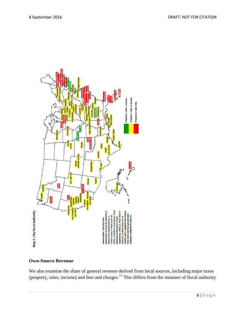
No state uniformly authorizes all three tax sources (see Map 1). The most common state fiscal
structure is one in which a state allows its cities to levy two local option taxes, typically a local
property tax and local sales tax (usually added on as an increment to the state sales tax). Some
states allow particular cities to levy some form of a third local option tax. For example, cities in
Alabama can levy a local option property tax and sales tax and a local option occupation tax (a
form of income tax) paid by those working in those cities. Birmingham has used the latter.
Cities in Missouri, New York, and Pennsylvania can levy special tax options (income tax in
Kansas City, St. Louis, New York City, and Yonkers, and a sales tax in Philadelphia).
Among the three major taxes, an incomes tax is used the least and, where authorized, they vary
in application and structure. Cities in Ohio and Kentucky can tax personal income at both the
place of employment and the place of business, making their income taxes a “commuter” tax as
well as a tax on residents. Moreover, Ohio and Kentucky cities can tax business profits at the
same rate as individual income. Cities in Washington State can impose a business and occupancy
(B&O) tax on all businesses (including services) that perform work or sell services within the
jurisdiction and on all incomes that are derived from working within the city. In other words, the
B&O tax operates much like a broad-based sales tax (including services) and income tax.15
Cities with the least fiscal autonomy (one local tax authority or no local tax autonomy) are in
many New England states, such as Boston, MA; Hartford, CT; and Providence, RI. These cities
only have access to a local property tax. Cities in Florida, Idaho, Mississippi, Nevada, Oregon,
and Wisconsin are also limited to a local property tax. Cities in Oklahoma only have access to a
local sales tax.16
8 September 2016 DRAFT: NOT FOR CITATION
8 | P a g e
Own-Source Revenue
We also examine the share of general revenue derived from local sources, including major taxes
(property, sales, income) and fees and charges.17
This differs from the measure of fiscal authority
8 September 2016 DRAFT: NOT FOR CITATION
9 | P a g e
in that it extends to how much cities rely on local sources.18
Having authority to levy a tax, for
instance, does not necessarily mean the tax is levied or structured to produce significant revenue.
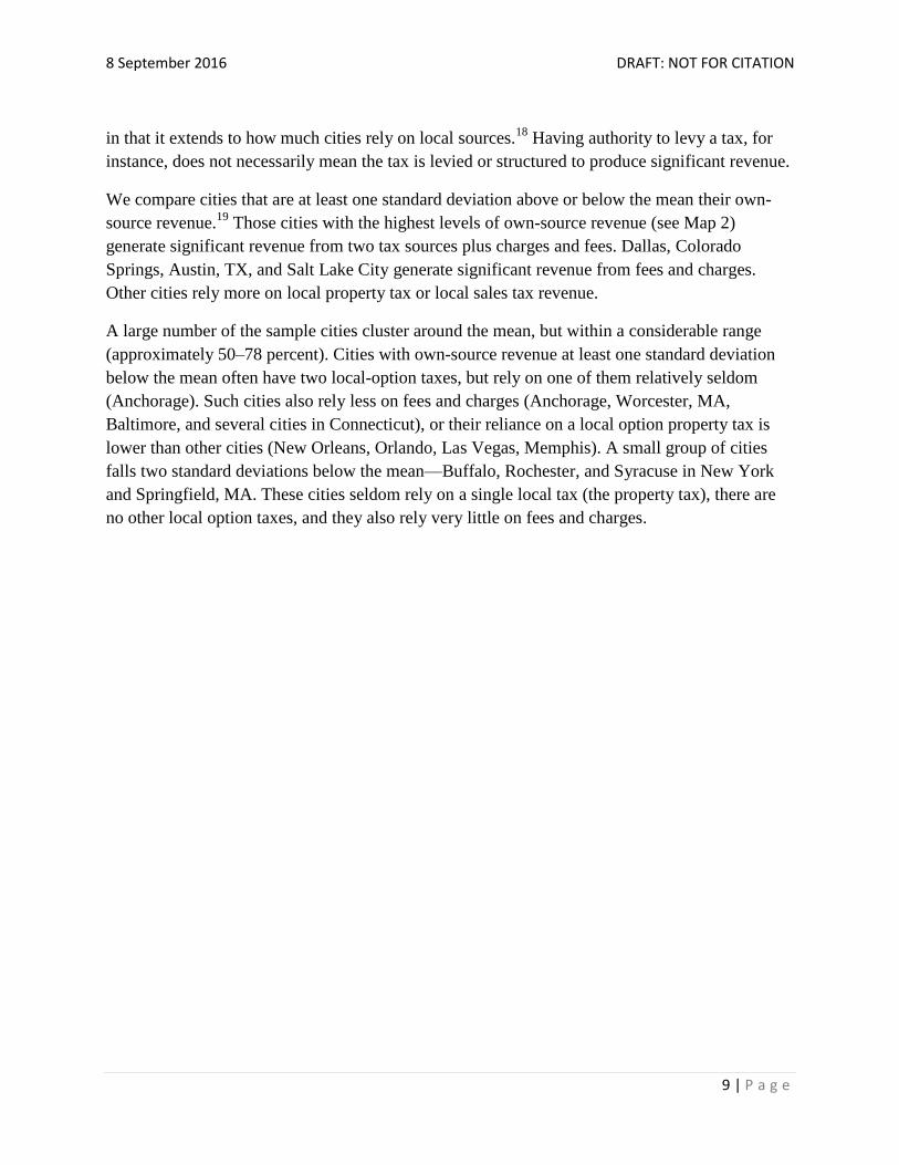
We compare cities that are at least one standard deviation above or below the mean their own-
source revenue.19
Those cities with the highest levels of own-source revenue (see Map 2)
generate significant revenue from two tax sources plus charges and fees. Dallas, Colorado
Springs, Austin, TX, and Salt Lake City generate significant revenue from fees and charges.
Other cities rely more on local property tax or local sales tax revenue.
A large number of the sample cities cluster around the mean, but within a considerable range
(approximately 50–78 percent). Cities with own-source revenue at least one standard deviation
below the mean often have two local-option taxes, but rely on one of them relatively seldom
(Anchorage). Such cities also rely less on fees and charges (Anchorage, Worcester, MA,
Baltimore, and several cities in Connecticut), or their reliance on a local option property tax is
lower than other cities (New Orleans, Orlando, Las Vegas, Memphis). A small group of cities
falls two standard deviations below the mean—Buffalo, Rochester, and Syracuse in New York
and Springfield, MA. These cities seldom rely on a single local tax (the property tax), there are
no other local option taxes, and they also rely very little on fees and charges.
8 September 2016 DRAFT: NOT FOR CITATION
10 | P a g e
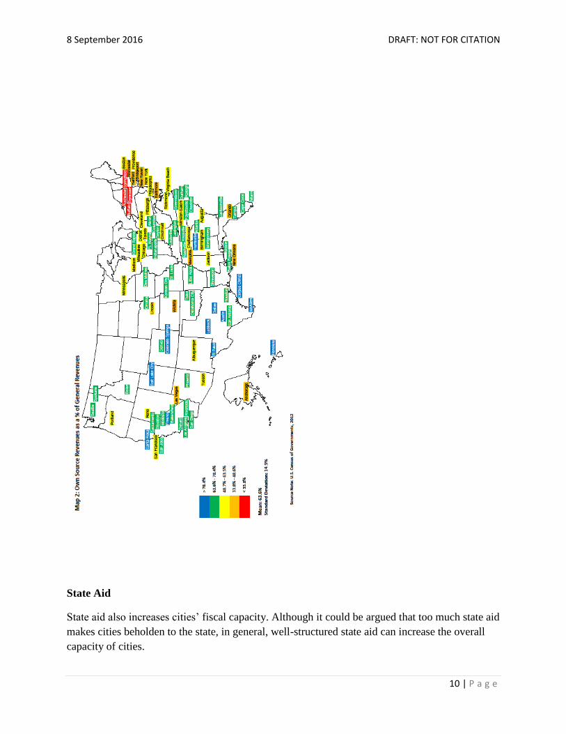
State Aid
State aid also increases cities’ fiscal capacity. Although it could be argued that too much state aid
makes cities beholden to the state, in general, well-structured state aid can increase the overall
capacity of cities.

8 September 2016 DRAFT: NOT FOR CITATION
11 | P a g e
We measure state aid to cities as the share of general revenue from state sources (direct state
aid), regardless of intent. In this case, we separate cities in states in which schools are dependent
units of city government because those cities receive substantially larger state assistance to help
cover school expenditures. Among this smaller group (see Table 1), those that rely most on state
aid—Buffalo, NY; Springfield, MA.; Rochester, NY; and New Haven, CT, for example—also
have significantly less own-source revenue, which not surprisingly makes them more reliant on
state assistance.
Table 1: State Aid as a Percentage of General Revenues (among cities with dependent
schools)
City State State Aid (%) SD
Buffalo NY 68.05 1
Springfield MA 65.68 1
Rochester NY 59.26 1
New Haven CT 58.82 1
Syracuse NY 54.54
Bridgeport CT 50.54
Worcester MA 47.58
Hartford CT 45.21
Anchorage AK 42.08
Baltimore MD 41.27
Providence RI 38.69
Memphis TN 35.27
Virginia Beach VA 32.42
Richmond VA 31.91
New York NY 29.04
Boston MA 28.09
Nashville TN 23.81 -1
Knoxville TN 13.64 -1
Chattanooga TN 8.11 -1
Mean
40.74
SD
16.15
Source: U.S. Census of Governments (2012)
Notes:
SD = standard deviation. "General Revenue" is used as defined by the U.S. Census of Governments, including
all local revenue except that from utilities and liquor store operations. The U.S. Census defines "General
Revenue" in broader terms than most cities' definitions. "State aid" is defined as general revenues that cities
receive from state governments. Data are missing for Charlotte, NC.

8 September 2016 DRAFT: NOT FOR CITATION
12 | P a g e
Among the larger group of cities without responsibility for schools, certain states stand out for
state assistance. Cities in Pennsylvania, Wisconsin, Arizona, and Ohio receive significantly
larger shares of state assistance (see Map 3) than others. In contrast, those in Texas and
California receive less state aid.
8 September 2016 DRAFT: NOT FOR CITATION
13 | P a g e
Tax and Expenditure Limits
Another way that state and local tax systems are constrained is through voter- or state-imposed
(constitutional or statutory) TELs. We examine two types of TELs: those that constrain the
property tax in particular and those that constrain overall revenue spending increases. Locally,
the most common TELs affect local property taxes, while effects on general revenue and
spending limits are less common.
There are three types of property tax limits: 1) those that seek to cap the property tax rate; 2)
those that seek to limit growth in local property assessments; and 3) those that seek to limit the
total levy (revenue) growth from property taxes from year to year. Not all of these limits are
individually binding in that raising assessments could circumvent a rate limit, or raising the
property tax could circumvent an assessment limit. We therefore make a distinction between
relatively “less (or non-) binding” and “potentially binding” property tax limits. Potentially
binding limits are those with either a levy limit (because it caps the bottom line level at which the
levy might increase) or some combination of rate and assessment limits together, thereby
negating the ability of localities to circumvent the limits. General revenue and spending limits
are considered potentially binding on their own given that they create caps on revenue or
spending growth.20
Sixty-three of the 100 sample cities have potentially binding limits in place
(see Map 4).
Twelve cities are unencumbered by TELs.21
Twenty-five cities confront nonbinding property tax
limits. The next tier, encompassing 41 cities, includes those constrained by potentially binding
property tax limits, in other words, those cities where a state TEL effectively caps or largely
restricts the local property tax. Lastly, 22 cities confront a combination of potentially binding
property tax limits and some form of limit on the annual growth of general revenues or
expenditures. It is worth noting that the existence of potentially binding TELs does not mean that
cities have no fiscal policy space available. Rather, it likely reduces the available space to
maneuver, limiting the range of fiscal decisions at the disposal of city leaders.

8 September 2016 DRAFT: NOT FOR CITATION
14 | P a g e
The Property Tax TEL Gap—TELs are an important factor in shaping the local fiscal
policy space, particularly those that limit local property tax authority and growth (and, therefore,
TEL are particularly important in cities that rely on property taxes as a major revenue source).
Most property tax TELs are imposed by state governments, but several cities also have imposed
8 September 2016 DRAFT: NOT FOR CITATION
15 | P a g e
TELs as additional constraints on local property taxes. Specific TEL terms and conditions vary
across states and over time. For example, California imposes a 2 percent limit on annual property
tax levy growth, whereas Pennsylvania, which also limits local property tax levies, sets the
growth limit at 10 percent. Property tax limits can also be amended.
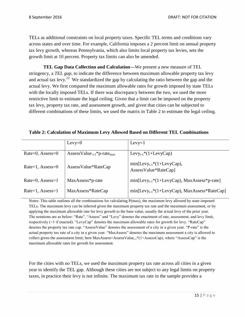
TEL Gap Data Collection and Calculation—We present a new measure of TEL
stringency, a TEL gap, to indicate the difference between maximum allowable property tax levy
and actual tax levy.22
We standardized the gap by calculating the ratio between the gap and the
actual levy. We first compared the maximum allowable rates for growth imposed by state TELs
with the locally imposed TELs. If there was discrepancy between the two, we used the more
restrictive limit to estimate the legal ceiling. Given that a limit can be imposed on the property
tax levy, property tax rate, and assessment growth, and given that cities can be subjected to
different combinations of these limits, we used the matrix in Table 2 to estimate the legal ceiling.
Table 2: Calculation of Maximum Levy Allowed Based on Different TEL Combinations
Levy=0 Levy=1
Rate=0, Assess=0 AssessValue t-1*p-ratemax Levyt-1*(1+LevyCap)
Rate=1, Assess=0 AssessValue*RateCap min[Levyt-1*(1+LevyCap),
AssessValue*RateCap]
Rate=0, Assess=1 MaxAssess*p-rate min[Levyt-1*(1+LevyCap), MaxAssess*p-rate]
Rate=1, Assess=1 MaxAssess*RateCap min[Levyt-1*(1+LevyCap), MaxAssess*RateCap]
Notes: This table outlines all the combinations for calculating P(max), the maximum levy allowed by state-imposed
TELs. The maximum levy can be inferred given the maximum property tax rate and the maximum assessment, or by
applying the maximum allowable rate for levy growth to the base value, usually the actual levy of the prior year.
The notations are as below: “Rate”, “Assess” and “Levy” denotes the enactment of rate, assessment, and levy limit,
respectively (=1 if enacted). “LevyCap” denotes the maximum allowable rates for growth for levy. “RateCap”
denotes the property tax rate cap. “AssessValue” denotes the assessment of a city in a given year. “P-rate” is the
actual property tax rate of a city in a given year. “MaxAssess” denotes the maximum assessment a city is allowed to
collect given the assessment limit; here MaxAssess=AssessValuet-1*(1+AssessCap), where “AssessCap” is the
maximum allowable rates for growth for assessment.
For the cities with no TELs, we used the maximum property tax rate across all cities in a given
year to identify the TEL gap. Although these cities are not subject to any legal limits on property
taxes, in practice their levy is not infinite. The maximum tax rate in the sample provides a

8 September 2016 DRAFT: NOT FOR CITATION
16 | P a g e
reasonable estimate for the highest possible level of tax levy. Using the same approach, we also
calculated the revenue gap for the cities subject to general revenue and expenditure limits.23
Negative TEL gap— There were many instances of a negative TEL gap. A TEL gap
becomes negative when an exemption allows cities to exceed existing limits. The distribution of
negative TEL gaps can shed light on the extent to which cities are exempted from TELs over
time. Of the 1,609 total observations, 652 (40 percent) had a negative TEL gap. Among these,
315 (that is, 40 cities in some years) had a TEL gap between 0 and -0.1, indicating these cities
exceeded their ceiling levy by 10 percent in these years. Another 177 (that is, 31 cities in some
years) had a TEL gap between -0.1 and -1, indicating that the actual levy exceeds the ceiling levy
by two times. Twelve cities had a TEL gap smaller than -1 (the actual levy is twice the ceiling).24
Four of these 12 cities are only subject to rate limits and thus it is possible for them to exceed the
ceiling levy by increasing property assessed values. The remaining eight cities are subject to
potentially binding TELs (a levy limit, or simultaneous rate and assessment limits), but it is
likely that there are TEL exemptions, or a related process, that allow the cities to exceed the
ceiling levy.
To examine the extent of TEL stringency, we divided the TEL gap into six brackets. The first
bracket includes all negative TEL gap cities—those cities that have exceeded the limits. The next
four brackets are 0–0.2, 0.2–0.3, 0.3–0.4, and 0.4–0.5. The last bracket includes all TEL gap with
values greater than 0.5. Figure 1 depicts the number of cities within each bracket and between
1995 and 2011. The number of cities in the first (less than zero) and second (0–0.2) brackets
increased, indicating that TELs became increasingly stringent after taking into account actual
property taxes levied. It also suggests that with time, more cities approached the legal levy limit,
or managed to exceed it through exemptions, voter override, or other processes.

8 September 2016 DRAFT: NOT FOR CITATION
17 | P a g e
Figure 1: Number of Cities by TEL Gap Bracket (1995-2011)
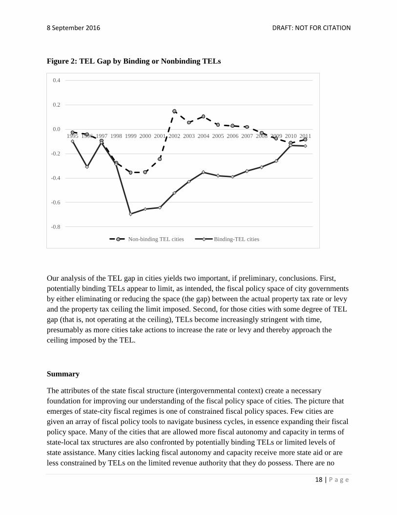
Interaction between TEL Gap and “Bindingness.”— We also identified an interaction
between the TEL gap and the degree to which a TEL binds the city’s ability to raise revenues. .
Nonbinding TELs, defined as imposing only a rate limit or only an assessment limit, can create
an abundant gap for property taxation because cities can circumvent the rate limit by raising
assessments or bypass the assessment limit by raising the property tax rates. Dividing cities into
binding and nonbinding groups, Figure 2 delineates the change in the average TEL gap between
1995 and 2011. We find that cities subject to nonbinding TELs or with no TELs had higher
average TEL gaps than cities with potentially binding limits. We also find higher TEL gap
averages between 2001 and 2007 for the cities with nonbinding limits, whereas the average TEL
gap for cities with potentially binding limits remains negative, pointing to less fiscal policy
space. Figure 2 suggests that potentially binding TELs are, in fact, more restrictive because they
limit the upside for additional property tax growth and, therefore, constrain the fiscal policy
space of cities confronted by those limits.
0
10
20
30
40
50
60
70
80
90
100
1995 1996 1997 1998 1999 2000 2001 2002 2003 2004 2005 2006 2007 2008 2009 2010 2011
L<0 0<L<0.2 0.2<L<0.3 0.3<L<0.4 0.4<L<0.5 L>0.5
8 September 2016 DRAFT: NOT FOR CITATION
18 | P a g e
Figure 2: TEL Gap by Binding or Nonbinding TELs
Our analysis of the TEL gap in cities yields two important, if preliminary, conclusions. First,
potentially binding TELs appear to limit, as intended, the fiscal policy space of city governments
by either eliminating or reducing the space (the gap) between the actual property tax rate or levy
and the property tax ceiling the limit imposed. Second, for those cities with some degree of TEL
gap (that is, not operating at the ceiling), TELs become increasingly stringent with time,
presumably as more cities take actions to increase the rate or levy and thereby approach the
ceiling imposed by the TEL.
Summary
The attributes of the state fiscal structure (intergovernmental context) create a necessary
foundation for improving our understanding of the fiscal policy space of cities. The picture that
emerges of state-city fiscal regimes is one of constrained fiscal policy spaces. Few cities are
given an array of fiscal policy tools to navigate business cycles, in essence expanding their fiscal
policy space. Many of the cities that are allowed more fiscal autonomy and capacity in terms of
state-local tax structures are also confronted by potentially binding TELs or limited levels of
state assistance. Many cities lacking fiscal autonomy and capacity receive more state aid or are
less constrained by TELs on the limited revenue authority that they do possess. There are no
-0.8
-0.6
-0.4
-0.2
0.0
0.2
0.4
1995 1996 1997 1998 1999 2000 2001 2002 2003 2004 2005 2006 2007 2008 2009 2010 2011
Non-binding TEL cities Binding-TEL cities
8 September 2016 DRAFT: NOT FOR CITATION
19 | P a g e
examples of cities with a combination of broad fiscal autonomy and capacity (in terms of own-
source revenue), greater state aid, and freedom from TELs. There are, in contrast, cities with
little or no fiscal autonomy, limited capacity, low levels of state aid, and potentially binding
TELs.
The structure of state-local systems fundamentally determines the extent to which cities’ fiscal
bases are well aligned with their economic bases, highlighted in a later section. In addition, state-
local fiscal structures interact with and are shaped by local political cultures, which determine
the demand for city services and willingness to provide city revenues (discussed later).
Expanding the fiscal policy space of cities will therefore require revisiting the issue of options
available within the context of state-local fiscal structures.

8 September 2016 DRAFT: NOT FOR CITATION
20 | P a g e
FPS Attribute 2: Alignment between Cities’ Economic Base and Fiscal
Base
The second FPS attribute is the extent to which the fiscal base of cities is well or poorly aligned
with their bases of economic activity. For instance, if the average income of a city’s residents
increases, one might conclude that the economic and fiscal bases of the city have improved. Yet,
if the city is unable to tax local incomes and other local option taxes remain stable, the city’s
fiscal health might hardly improve at all. We present a “fiscal base” measure that is meant to
more accurately represent the extent to which a city’s fiscal levers overlay the growth sectors of
the city’s economy.
The evolution of municipal revenue structure was largely a response to the changing political
climate and legal constraints on municipal revenue. The evolution of municipal revenue systems,
however, does not reflect the changing economic bases of cities, which have undergone
significant changes in recent decades. As a result, municipal revenue structures have gradually
become disconnected from their economic bases. This misalignment has undermined the fiscal
capacity of municipal governments to raise adequate resources and fund investment and services
at appropriate levels.
Our analysis seeks to reconnect the two. Using economic and fiscal data from 100 large U.S.
cities, we first calculated the constant dollar value of three economic components: per capita
market value of properties, per capita value of retail sales, and per capita income.25
We
aggregated the three measures and calculated the share of each component in the aggregate
economic base. Then we compared each economic base share with the share of tax revenue
collected from that source.
The comparison shows quite substantial differences between taxes and the economic bases. For
instance, in Mobile, AL, in 2010, the per capita value of properties was 60 percent of its
aggregate economic base, but the local property tax only contributed 10 percent total tax
revenue. Similarly, the shares of per capita value of properties were 63 percent and 61 percent in
Colorado Springs and Oklahoma City, respectively, in 2010, but the shares of property tax
revenue were just 15 percent and 16 percent, respectively. On the other hand, in Wichita, KS;
Jackson, MS; Rochester, NY; and Buffalo, NY, per capita values of properties were less than 60
percent of their aggregate economic bases, but property taxes accounted for 100 percent of tax
revenue in 2010. The average shares of per capita value of properties and property taxes were 64
and 67 percent, respectively, for the 100 sample cities in 2010.
A similar pattern of misalignment is evident for local sales taxes. In 2007, some cities had
significant per capita retail sales (above 20 percent in Fort Wayne, IN and Jackson, MS) but very
low shares of sales taxes (zero in Fort Wayne and Jackson). Other cities had quite large shares of

8 September 2016 DRAFT: NOT FOR CITATION
21 | P a g e
sales tax revenue (88 percent in Colorado Springs and 92 percent in Mobile) but relatively small
shares of per capita value of retail sales (14 percent for Colorado Springs and 19 percent for
Mobile). The average shares of per capita value of retail sales and sales tax were 12 percent and
24 percent, respectively, for the sample cities in 2007.
The misalignment of municipal tax structure with cities’ economic base is the result of changing
economic conditions coupled with a largely politically driven evolution of municipal tax
structures. The substantial gaps between the share of tax revenue and the share of cities’ tax base
reflect municipalities’ varying access to different components of the economic base for revenue.
The restricted access to revenue results in structural imbalance between revenue-raising capacity
and spending need.
A City’s Fiscal Base
A city’s ability to transform its economic base into government revenue depends on the types of
legal taxing authorities and state-imposed constraints on revenue. Therefore, we introduce fiscal
base to better reflect the extent of alignment between a city’s revenue structure and its
underlying economic base. We define municipal fiscal base as the aggregate economic activities
from which cities can draw to finance public services. In other words, a fiscal base is the
economic base that a city government can tax. The definition not only reflects the connection
between economic conditions and revenue raising potential, but it also highlights the restrictive
nature of relevant state laws and statues on municipal access to various revenue sources.
The fiscal base value is defined as the weighted average of the three economic base components:
per capita market value of properties, per capita value of retail sales, and per capita income. We
use the share of the aggregate broad-based taxes from a particular source (property tax, sales tax,
income tax) as the weight of that economic tax base, and we calculate the fiscal base value as a
weighted average of the three tax bases. For instance, if property tax accounts for 60 percent of
total local tax revenue, the per capita property value will be multiplied by 60 percent.
We calculate the fiscal base for 93 sample cities in 2000 and 2010. Some cities are excluded
because of missing data. We find wide variations in fiscal bases across the cities. In both 2000
and 2010, the fiscal base values are above $100,000 for four cities: Orlando, FL; Honolulu, HI;
Portland, OR; and Atlanta, GA. Five cities have fiscal bases below $30,000 in both years,
including Oklahoma City, Mobile, AL; Buffalo, NY; Colorado Springs, CO; and Tulsa, OK. The
median values of the fiscal base are $44,733 in 2000 and $54,195 in 2010. Minimum values are
$22,049 and $22,613, respectively. Maximum values are $162,319 and $170,643.
Between 2000 and 2010, the fiscal base grew in 67 cities (some significantly) and declined in 26
cities. Three cities doubled their fiscal base in this 10-year period, including San Diego, CA,
from $40,357 to $98,697; Miami, FL, from $57,355 to $126,547; and Oxnard, CA, from $26,811
to $59,214. However, five cities saw a decline of more than 20 percent in their fiscal base in the
8 September 2016 DRAFT: NOT FOR CITATION
22 | P a g e
same period. These cities are Winston-Salem, NC, from $95,102 to $75,277; Greensboro, NC,
from $98,030 to $74,270; Charlotte, NC, from $115,172 to $78,882; Fayetteville, NC, from
$72,984 to $46,504; and Boise, ID, from $120,158 to $71,635. The median growth rate during
the period was 17.4 percent.
Fiscal Base Rankings
For cities with similar tax structures, their fiscal base rankings are based on three tax bases, and
particularly the property tax base. The figures show the relative magnitude of each per capita tax
base (measured by the distance from origin to the intersection of the blue triangle with each axis)
and the relative magnitude of the reliance ratio on each broad based tax (measured by the
distance from the origin to the intersection of the orange triangle with each axis). The numbers 1,
2 and 3 on the triangle points differentiate property tax base (ratio), sales tax base (ratio) and
income tax base (ratio). The other decimal numbers only show relative scales without much
practical meaning.
For instance, Buffalo, NY, and Orlando, FL, are two of 23 cities that relied solely on property tax
in 2010. Orlando’s fiscal base is ranked 1st because its per capita property values are
approximately $171,000 compared with $25,000 in Buffalo, which as ranked 91st in 2010 (see
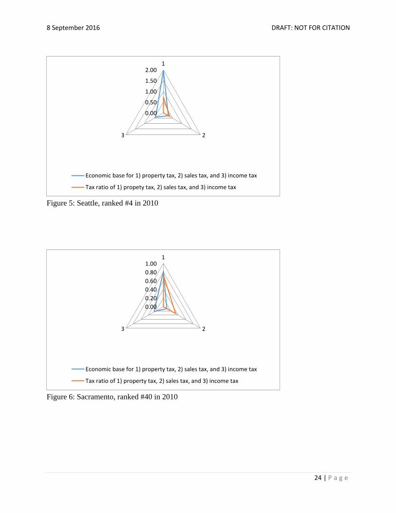
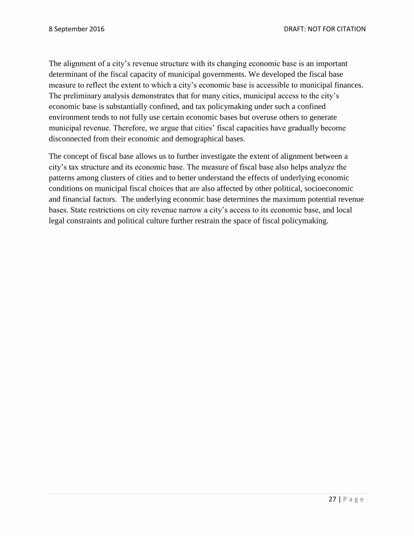
Figures 3 and 4). Seattle and Sacramento are also similar in tax structure (deriving about 73
percent from property tax and 27 percent from sales tax). Yet they have quite different fiscal
bases (Seattle was ranked 4th
and Sacramento 40th
in 2010) because Seattle has much larger
property and sales tax bases ($197,000 and $27,000 per capita, respectively) than Sacramento at
$82,000 and $10,000, respectively (see Figures 5 and 6).
A large fiscal base is the result of a high valued tax base coupled with a high reliance on that tax
revenue. As a result, two cities with similarly valued tax bases may have quite different fiscal
bases if their tax structures are different. For instance, as shown in Figures 7 and 8, Boston and
Denver had similar per capita property values in 2010 ($137,000 and $134,000, respectively).
They also had similar per capita retail sales in 2007 ($11,500 and $11,900, respectively), and
similar per capita personal incomes in 2010 ($32,000 and $31,000). Yet Boston’s 2010 fiscal
base is much higher (7th) than Denver’s (42nd) because Boston relies much more on property
tax (100 percent) than Denver (40 percent). Although Denver also collects about 60 percent of its
tax revenue from municipal sales taxes, the sales tax base is much smaller than the property tax
base. Likewise for Tampa, FL, and Huntsville, AL (see Figures 9 and 10). Both cities share
similar per capita property values and retail sales. But because Tampa relies primarily on
property taxes and Huntsville relies more on sales taxes, Tampa ranks much higher (12th) on its
fiscal base than Huntsville (59th).

8 September 2016 DRAFT: NOT FOR CITATION
23 | P a g e
Figure 3: Orlando, ranked #1 in 2010
Figure 4: Buffalo, ranked #91 in 2010
0.00
0.50
1.00
1.50
2.001
23
Economic base for 1) property tax, 2) sales tax, and 3) income tax
Tax ratio of 1) property tax, 2) sales tax, and 3) income tax
0.00
0.20
0.40
0.60
0.80
1.001
23
Economic base for 1) property tax, 2) sales tax, and 3) income tax
Tax ratio of 1) property tax, 2) sales tax, and 3) income tax
8 September 2016 DRAFT: NOT FOR CITATION
24 | P a g e
Figure 5: Seattle, ranked #4 in 2010
Figure 6: Sacramento, ranked #40 in 2010
0.00
0.50
1.00
1.50
2.001
23
Economic base for 1) property tax, 2) sales tax, and 3) income tax
Tax ratio of 1) propety tax, 2) sales tax, and 3) income tax
0.00
0.20
0.40
0.60
0.80
1.001
23
Economic base for 1) property tax, 2) sales tax, and 3) income tax
Tax ratio of 1) property tax, 2) sales tax, and 3) income tax

8 September 2016 DRAFT: NOT FOR CITATION
25 | P a g e
Figure 7: Boston, ranked #7 in 2010
Figure 8: Denver, ranked #42 in 2010
0.00
0.50
1.00
1.501
23
Economic base for 1) property tax, 2) sales tax, and 3) income tax
Tax ratio of 1) property tax, 2) sales tax, and 3) income tax
0.00
0.50
1.00
1.501
23
Economic base for 1) property tax, 2) sales tax, and 3) income tax
Tax ratio of 1) property tax, 2) sales tax, and 3) income tax

8 September 2016 DRAFT: NOT FOR CITATION
26 | P a g e
Figure 9: Tampa, ranked #12 in 2010
Figure 10: Huntsville, ranked #59 in 2010
0.000.200.400.600.801.001.20
1
23
Economic base for 1) property tax, 2) sales tax, and 3) income tax
Tax ratio of 1) property tax, 2) sales tax, and 3) income tax
0.000.200.400.600.801.001.20
1
23
Economic base for 1) property tax, 2) sales tax, and 3) income tax
Tax ratio of 1) property tax, 2) sales tax, and 3) income tax
8 September 2016 DRAFT: NOT FOR CITATION
27 | P a g e
The alignment of a city’s revenue structure with its changing economic base is an important
determinant of the fiscal capacity of municipal governments. We developed the fiscal base
measure to reflect the extent to which a city’s economic base is accessible to municipal finances.
The preliminary analysis demonstrates that for many cities, municipal access to the city’s
economic base is substantially confined, and tax policymaking under such a confined
environment tends to not fully use certain economic bases but overuse others to generate
municipal revenue. Therefore, we argue that cities’ fiscal capacities have gradually become
disconnected from their economic and demographical bases.
The concept of fiscal base allows us to further investigate the extent of alignment between a
city’s tax structure and its economic base. The measure of fiscal base also helps analyze the
patterns among clusters of cities and to better understand the effects of underlying economic
conditions on municipal fiscal choices that are also affected by other political, socioeconomic
and financial factors. The underlying economic base determines the maximum potential revenue
bases. State restrictions on city revenue narrow a city’s access to its economic base, and local
legal constraints and political culture further restrain the space of fiscal policymaking.

8 September 2016 DRAFT: NOT FOR CITATION
28 | P a g e
FPS Attribute 3: Local Political Demand
The third FPS attribute addresses the variation among cities in demands on government services
and local political culture. The higher the demands, the less likely city leaders can expand or
provide additional services, unless higher demands are coupled with greater acceptance of higher
taxes. For example, the Great Recession put pressure on many cities to provide more social
services. However, at the same time, the public recognized that services would likely decrease
amid declining fiscal conditions. We present a new measure of “demand” as a means of
exploring the impact of citizen demands on the fiscal policymaking behavior of city officials.
As an essential dimension of the FPS, the local political demand attribute—its conceptualization
and operationalization—is unique and enables a greater understanding of the tension that local
fiscal policymakers can feel as a result of local political demands. The elephant in the room for
any locality is the local political culture and its dynamic interaction with the demands and
preferences of its citizens. Essentially, this attribute formalizes the interaction of how local
political ideology, interests, culture, and institutions of a community act to constrain or widen
fiscal decision-making options.
Measuring the Local Political Space
It is not possible to “cleanly” separate the elements of local politics; instead, this FPS attribute
comprises a limited number of summary measures of city politics that encapsulate various
influences on fiscal policy.
The local political demand includes:
1. The partisanship or ideology of the local population, which primarily refers to the
rightward or leftward tilt of voters (or those who might sometimes choose to vote) in the
area; and
2. Resident and interest‐group demands, which may be thought of as the bottom‐up
pressures facing local policymakers from various constituencies, whether organized or
unorganized.
Partisanship or Ideology of the Local Population— The strength of political party leanings
is not always theorized as an essential component of local fiscal policy in comparison to
federalism, economic competition, and leadership. However, we cannot ignore that in local
politics just as in national politics, party allegiances underlie policy preferences. Democratic
tendencies are associated with more expansive fiscal policies and with allegiances to public
employees, the poor, and minorities, whereas Republican leanings are associated with fiscal
8 September 2016 DRAFT: NOT FOR CITATION
29 | P a g e
conservatism, a presupposition against tax increases, and allegiance to a good business climate
and businesslike efficiencies in government.
As such, we expect significant differences between left‐leaning (more Democratic) and right‐
leaning (more Republican) cities in their approaches to fiscal reform and financial adjustments.
We rank local political ideology on a simulated scale from liberal (low negative values) to
conservative (high positive values); for the FPS sample of cities, the 2002 local political
ideology scale ranged from -0.96 to 0.32, and the 2002 local political ideology scale ranged from
-1.02 – 0.24.26
Liberal cities, particularly those with high union coverage, will tend to experience
pressures in favor of increasing or maintaining per capita spending levels and levels of public
employment. Depending on one’s perspective (and on whether economic times are bountiful or
poor), this might be viewed as either a constraint on fiscal reform or an opportunity for new sorts
of programmatic commitments.
Resident and Interest‐Group Demands—The local public sector is where local
demands and interests are translated into public policy decisions and public services.27
Both
resident demands and other interest group demands can affect fiscal policy decision-making
differently and thus are two separate concepts in measuring the local political space.
We use housing affordability to represent resident demands. We capture local resident demands
in a rent-to-income ratio.28
Housing affordability has been shown to predict certain orientations
to residential policy among city officials, who were apparently cognizant of residents’
affordability problems.29
Homeowners are generally thought to be more sensitive than renters to
increases in local taxes or indebtedness (given homeowners pay property taxes), whereas renters,
low‐income households, and racial minorities are often thought to hold more fiscally
expansionary views. Local resident demands are represented in a rent-to-income ratio, a measure
of unaffordability of rental housing in the city, where higher values indicate greater rental
housing unaffordability.30
Interest groups’ influence on the local political space focuses on public‐sector unions (or other
associations of municipal employees), who bargain for or protest against particular types of fiscal
changes. We use the percentage of public‐sector workers covered by a collective bargaining
agreement in a metropolitan area in a given year to represent interest group demands.31
Cities
with a larger percentage of public‐sector unionized workers will tend to exact pressure on fiscal
policymakers for certain types of fiscal changes, such as less contracting or outsourcing of
services. In addition, more public sector unionization should generate more pressure to retain
existing spending commitments (especially for personnel) and support higher taxes and more
revenue. Thus, the effect can both constrain and expand the fiscal decision-making process.
8 September 2016 DRAFT: NOT FOR CITATION
30 | P a g e
Local Political Demand Space
Together with the other FPS attributes, local ideology, public unionism, and housing
affordability might well have interactive, contingent, and nonlinear effects on fiscal
policymaking. The demand scale is the summary measurement of this dynamic interaction that
represents the political pressure for fiscally expansionary policy in each city. High values on the
demand scale indicate greater pressure, which would make fiscal load‐shedding, contracting out,
or austerity policies more difficult. Low (negative) values indicate less fiscally expansionary
pressure.32
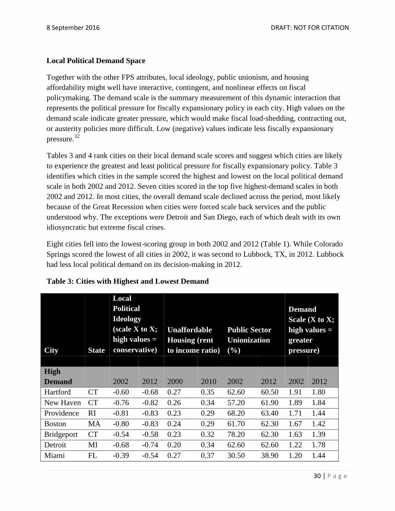
Tables 3 and 4 rank cities on their local demand scale scores and suggest which cities are likely
to experience the greatest and least political pressure for fiscally expansionary policy. Table 3
identifies which cities in the sample scored the highest and lowest on the local political demand
scale in both 2002 and 2012. Seven cities scored in the top five highest-demand scales in both
2002 and 2012. In most cities, the overall demand scale declined across the period, most likely
because of the Great Recession when cities were forced scale back services and the public
understood why. The exceptions were Detroit and San Diego, each of which dealt with its own
idiosyncratic but extreme fiscal crises.
Eight cities fell into the lowest-scoring group in both 2002 and 2012 (Table 1). While Colorado
Springs scored the lowest of all cities in 2002, it was second to Lubbock, TX, in 2012. Lubbock
had less local political demand on its decision-making in 2012.
Table 3: Cities with Highest and Lowest Demand
City State
Local
Political
Ideology
(scale X to X;
high values =
conservative)
Unaffordable
Housing (rent
to income ratio)
Public Sector
Unionization
(%)
Demand
Scale (X to X;
high values =
greater
pressure)
High
Demand 2002 2012 2000 2010 2002 2012 2002 2012
Hartford CT -0.60 -0.68 0.27 0.35 62.60 60.50 1.91 1.80
New Haven CT -0.76 -0.82 0.26 0.34 57.20 61.90 1.89 1.84
Providence RI -0.81 -0.83 0.23 0.29 68.20 63.40 1.71 1.44
Boston MA -0.80 -0.83 0.24 0.29 61.70 62.30 1.67 1.42
Bridgeport CT -0.54 -0.58 0.23 0.32 78.20 62.30 1.63 1.39
Detroit MI -0.68 -0.74 0.20 0.34 62.60 62.60 1.22 1.78
Miami FL -0.39 -0.54 0.27 0.37 30.50 38.90 1.20 1.44

8 September 2016 DRAFT: NOT FOR CITATION
31 | P a g e
Low
Demand 2002 2012 2000 2010 2002 2012 2002 2012
Ft. Wayne IN 0.15 0.06 0.16 0.17 66.00 27.90 -0.42 -1.11
Lubbock TX 0.27 0.24 0.19 0.22 14.30 0.00 -1.00 -1.39
Virginia
Beach VA 0.32 0.19 0.18 0.22 22.40 12.70 -1.04 -1.08
Wichita KS 0.00 -0.03 0.15 0.18 23.30 28.60 -1.08 -0.97
Winston-
Salem NC 0.02 -0.16 0.17 0.20 9.90 13.00 -1.09 -0.85
Lincoln NE 0.06 -0.05 0.15 0.17 23.60 -1.13 -1.25
Huntsville AL 0.11 0.14 0.14 0.17 16.10 35.10 -1.40 -1.07
Colorado
Springs CO 0.31 0.18 0.17 0.17 15.50 24.50 -1.42 -1.29
Table 4: Local Political Demand Scale Ranking of Sample Cities
City State Demand Scale 2002 Demand Scale 2012
Hartford CT 1.91 1.80
New Haven CT 1.89 1.84
Providence RI 1.71 1.44
Boston MA 1.67 1.42
Bridgeport CT 1.63 1.39
Syracuse NY 1.49 0.93
Buffalo NY 1.49 1.30
New York NY 1.40 1.33
Rochester (NY) NY 1.37 1.39
San Francisco CA 1.32 1.26
Detroit MI 1.22 1.78
Miami FL 1.20 1.44
Los Angeles CA 1.09 1.03
Philadelphia PA 1.06 1.05
Santa Rosa CA 0.92 0.72
Cleveland OH 0.91 1.01
Springfield (MA) MA 0.83 0.94
Seattle WA 0.76 0.64
Minneapolis MN 0.74 0.53

8 September 2016 DRAFT: NOT FOR CITATION
32 | P a g e
Baltimore MD 0.72 0.62
Pittsburgh PA 0.71 0.58
Chicago IL 0.67 0.65
Sacramento CA 0.64 0.62
New Orleans LA 0.63 0.76
San Diego CA 0.51 0.60
Milwaukee WI 0.39 0.52
Portland (OR) OR 0.38 0.42
Madison WI 0.37 -0.15
St. Louis MO 0.35 0.51
Worcester MA 0.33 0.42
San Jose CA 0.30 0.44
Stockton CA 0.26 0.80
Richmond VA 0.25 0.34
Memphis TN 0.23 0.01
Akron OH 0.22 0.09
Dayton OH 0.20 -0.06
Birmingham AL 0.19 0.17
Riverside CA 0.19 0.44
Honolulu HI 0.18 0.42
Orlando FL 0.13 -0.12
Spokane WA 0.10 -0.11
Fresno CA 0.09 0.08
Oxnard CA 0.06 0.09
Atlanta GA 0.05 -0.14
Toledo OH 0.01 0.20
Modesto CA -0.01 0.23
Denver CO -0.03 -0.09
Tampa FL -0.05 -0.03
Cape Coral FL -0.08 -0.43
Cincinnati OH -0.09 -0.18
Columbus (OH) OH -0.11 0.02
Austin TX -0.11 -0.15
Grand Rapids MI -0.18 0.16
Tucson AZ -0.18 -0.36
Kansas City (MO) MO -0.19 -0.24
Anchorage AK -0.27 -0.99
Las Vegas NV -0.28 -0.14

8 September 2016 DRAFT: NOT FOR CITATION
33 | P a g e
Des Moines IA -0.30 -0.32
Louisville KY -0.32 -0.59
Reno NV -0.34 -0.18
Durham NC -0.39 -0.41
Tulsa OK -0.40 -0.82
Albuquerque NM -0.41 -0.59
Dallas TX -0.41 -0.16
Ft. Wayne IN -0.42 -1.11
Houston TX -0.49 -0.41
Bakersfield CA -0.49 -0.33
Baton Rouge LA -0.51 -0.33
Salt Lake City UT -0.53 -0.79
Shreveport LA -0.55 -0.71
McAllen TX -0.56 -0.73
Greensboro NC -0.56 -0.36
Mobile AL -0.58 -0.55
Little Rock AR -0.60 -0.88
Phoenix AZ -0.63 -0.69
Indianapolis IN -0.66 -0.54
Jackson MS -0.67 -0.10
Knoxville TN -0.68 -0.57
Raleigh NC -0.69 -0.72
Nashville TN -0.71 -0.79
Chattanooga TN -0.72 -0.83
Jacksonville FL -0.72 -0.67
Montgomery AL -0.78 -0.32
Boise ID -0.79 -0.84
Corpus Christi TX -0.83 -0.71
Charlotte NC -0.83 -0.83
El Paso TX -0.85 -0.69
San Antonio TX -0.85 -0.65
Omaha NE -0.86 -0.94
Lexington KY -0.88 -0.75
Augusta (GA) GA -0.91 -0.24
Fayetteville (NC) NC -0.98 -0.94
Lubbock TX -1.00 -1.39
Virginia Beach VA -1.04 -1.08
Oklahoma City OK -1.06 -0.97
8 September 2016 DRAFT: NOT FOR CITATION
34 | P a g e
Wichita KS -1.08 -0.97
Winston-Salem NC -1.09 -0.85
Lincoln NE -1.13 -1.25
Huntsville AL -1.40 -1.07
Colorado Springs CO -1.42 -1.29
Note: Ideology, a component of the summary scale, was inverted for the Demand Scale calculation, per description
in text. However, in this section and for all figures and tables, Demand Scale is not inverted as it is for the fiscal, tax,
demand, and gap analysis in the “Putting It Altogether” section.
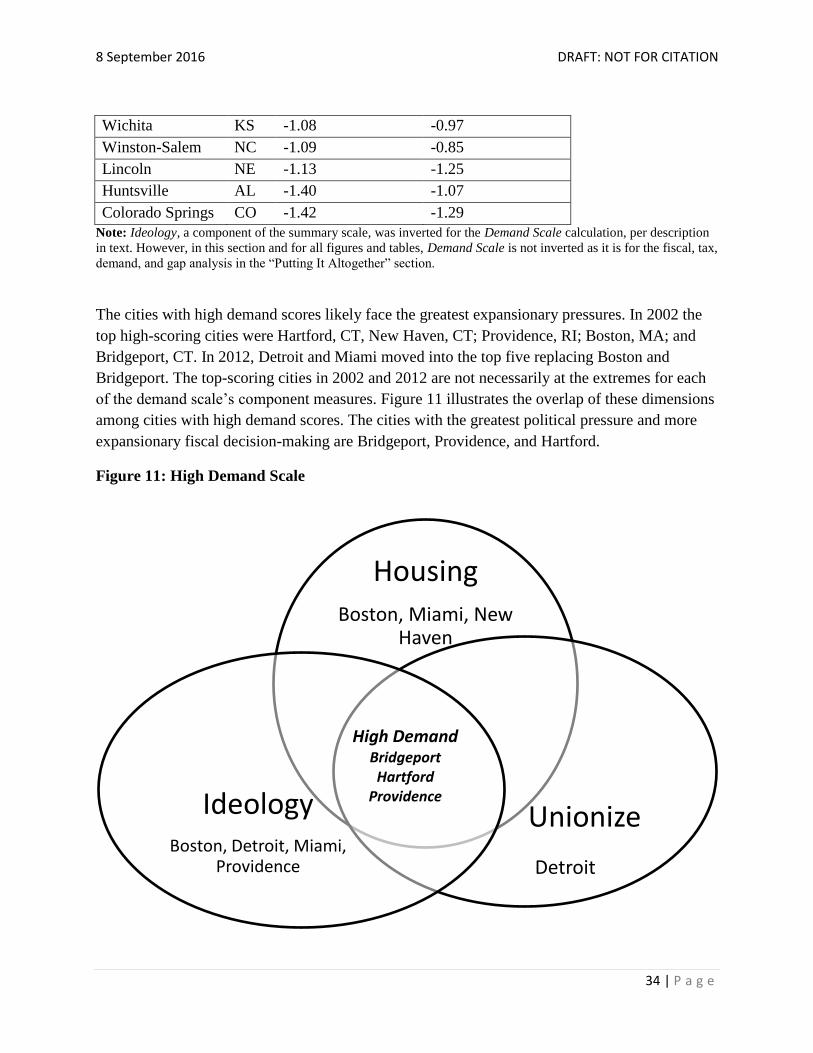
The cities with high demand scores likely face the greatest expansionary pressures. In 2002 the
top high-scoring cities were Hartford, CT, New Haven, CT; Providence, RI; Boston, MA; and
Bridgeport, CT. In 2012, Detroit and Miami moved into the top five replacing Boston and
Bridgeport. The top-scoring cities in 2002 and 2012 are not necessarily at the extremes for each
of the demand scale’s component measures. Figure 11 illustrates the overlap of these dimensions
among cities with high demand scores. The cities with the greatest political pressure and more
expansionary fiscal decision-making are Bridgeport, Providence, and Hartford.
Figure 11: High Demand Scale
Housing Boston, Miami, New
Haven
Unionize
Detroit
Ideology Boston, Detroit, Miami,
Providence
High Demand Bridgeport Hartford
Providence

8 September 2016 DRAFT: NOT FOR CITATION
35 | P a g e
The cities with the least political pressure for expansionary policies in 2000 were Wichita, KS;
Winston-Salem, NC; Lincoln, NE; Huntsville, AL; and Colorado Springs, CO. In 2012, Virginia
Beach, VA: Ft. Wayne, IN; and Lubbock, TX, replaced Wichita, Winston-Salem, and Huntsville.
Overall, the cities expected to have the least political pressure and expansionary fiscal policy are
Colorado Springs and Huntsville (Figure 12).
Figure 12: Low Demand Scale
Case Study: Providence
Providence is a perfect example of the types of expansionary fiscal pressures that a city can
experience. Providence was hit hard by the Great Recession. Employment declined significantly,
particularly in manufacturing, which, given its ongoing 30-year decline, has resulted in a low per
capita income as the workforce transferred from manufacturing to the lower-paying service
industry.
Housing Ft.Wayne, Lincoln, Lubbock, Wichita,
Winston-Salem
Unionize Lubbock
Winston-Salem
Ideology Ft. Wayne, Lubbuck, Virginia
Beach
Low Demand Colorado Springs
Huntsville
8 September 2016 DRAFT: NOT FOR CITATION
36 | P a g e
In addition, Providence’s fiscal architecture is not as well aligned with its fiscal base. Beyond the
pressure of lower earnings among its residents, Providence relies heavily on property taxes,
ranging from 35 to 57 percent of total revenue. However, properties have low market and
assessed values compared with most constrained FPS cities. The fiscal reliance is compounded
because nearly 40 percent of the city’s property is tax-exempt, owned by more than 3,000
nonprofit organizations, such as the universities and hospitals that are eight of the ten largest
employers in Providence.33
The assessed value of this property is said to be more than $3
billion.34
Providence also relies on state aid (which has in the past been reduced by 50 percent),
and in 2009, the state legislature eliminated general revenue sharing payments to all
municipalities. Finally, in 2007, the state passed more stringent TEL legislation that limited levy
increases and required a city’s governing body to secure an 80 percent majority to increase the
tax cap.35
Thus, Providence is restricted by a misaligned fiscal architecture compounded by TEL
restrictions.
This fiscal misalignment, however, confronts great local political demand for fiscal expansion.
Providence’s expenditures on public safety have remained steady as did expenditures for public
works, though still low among constrained FPS cities. In 2009, Mayor David Cicilline’s
proposed $7.1 million budget reduction included a wage freeze for unionized employees,
estimated to save $12 million. He also proposed eliminating 30 vacant fire positions to save
another $3 million. After tense negotiations with the fire union, both sides came to a tentative
agreement that froze wages for 2010 and 2011 and reduced 31 positions by way of attrition.36
A
few years later in 2011, Mayor Angel Taveras sought to cut the police force by 78 positions, but
contract negotiations resulted in only 30-40 early retirements and the elimination of 26 unfilled
vacant positions. Thus, in 2011, the number of law enforcement employees reached a two-decade
low of 428 compared with 494 in mid-2009.
The effect of local political demand in combination with fiscal and intergovernmental limitations
is evident in Providence. Providence experienced declining housing affordability and became
more liberal during the decade. Strong unionization made it difficult to reduce municipal
employment even though it would create savings. The policy actions suggest that Providence is
in a desperate need of breathing room.
8 September 2016 DRAFT: NOT FOR CITATION
37 | P a g e
Pathways of Adjustment: How the Fiscal Policy Space Shaped Cities’
Recent Fiscal Policy Responses
We posit that the three FPS attributes fundamentally shape the fiscal policy actions—the
pathways of adjustment—that city leaders employ when encountering changing economic and
fiscal conditions, whether an external shock (e.g., the Great Recession) or a period of marked
economic growth. Here we begin to examine the interaction of cities’ FPS and their fiscal
pathways of adjustment to identify any patterns that can inform a more detailed and robust
analysis of how the FPS of cities drives policy action.
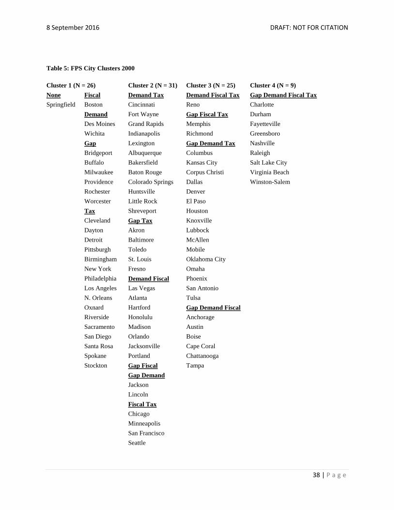
We cluster cities on the basis of four FPS attributes.37
We then categorized cities by creating
dummy variables that designate cities in the following manner:
Fiscal Base (FISCAL) denotes cities with a fiscal base measure above the mean, indicating
cities with fiscal architectures that are better aligned with their underlying fiscal base. Cities
below the mean do not receive the "Fiscal" designation (see Tables 5 and 6).
Demand Pressure (DEMAND) denotes cities with a local political demand scale measure above
the mean, indicating that cities with fewer local political demands. Cities below the mean
do not receive the “Demand” designation.
Tax Authorization (TAX) denotes cities with access to more than a local property tax, either a
local sales tax, or local income tax, or both. Cities with access only to a property tax
do not receive the "Tax" designation.
Property Tax Gap (GAP) denotes cities with the ability to increase their local property tax levy,
within the space allowed by property tax TELs. Cities lacking this ability, and which are
therefore operating at their maximum property tax levy, do not receive the "Gap” designation.
8 September 2016 DRAFT: NOT FOR CITATION
38 | P a g e
Table 5: FPS City Clusters 2000
Cluster 1 (N = 26) Cluster 2 (N = 31) Cluster 3 (N = 25) Cluster 4 (N = 9)
None Fiscal Demand Tax Demand Fiscal Tax Gap Demand Fiscal Tax
Springfield Boston Cincinnati Reno Charlotte
Demand Fort Wayne Gap Fiscal Tax Durham
Des Moines Grand Rapids Memphis Fayetteville
Wichita Indianapolis Richmond Greensboro
Gap Lexington Gap Demand Tax Nashville
Bridgeport Albuquerque Columbus Raleigh
Buffalo Bakersfield Kansas City Salt Lake City
Milwaukee Baton Rouge Corpus Christi Virginia Beach
Providence Colorado Springs Dallas Winston-Salem
Rochester Huntsville Denver
Worcester Little Rock El Paso
Tax Shreveport Houston
Cleveland Gap Tax Knoxville
Dayton Akron Lubbock
Detroit Baltimore McAllen
Pittsburgh Toledo Mobile
Birmingham St. Louis Oklahoma City
New York Fresno Omaha
Philadelphia Demand Fiscal Phoenix
Los Angeles Las Vegas San Antonio
N. Orleans Atlanta Tulsa
Oxnard Hartford Gap Demand Fiscal
Riverside Honolulu Anchorage
Sacramento Madison Austin
San Diego Orlando Boise
Santa Rosa Jacksonville Cape Coral
Spokane Portland Chattanooga
Stockton Gap Fiscal Tampa
Gap Demand
Jackson
Lincoln
Fiscal Tax
Chicago
Minneapolis
San Francisco
Seattle

8 September 2016 DRAFT: NOT FOR CITATION
39 | P a g e
Table 6: FPS City Clusters in 2010
Cluster1 (N = 18) Cluster 2 (N = 32) Cluster 3 (N = 30) Cluster 4 (N = 11)
None Fiscal Demand Tax Demand Fiscal
Tax
Gap Demand Fiscal
Tax
Milwaukee Boston Dayton Little Rock Charlotte
Springfield Worcester Fort Wayne Gap Fiscal Tax Dallas
Demand Indianapolis Richmond Durham
Des Moines Albuquerque San Diego Greensboro
Gap Baton Rouge Santa Rosa Knoxville
Buffalo Huntsville Gap Demand Tax Nashville
Hartford Shreveport Cincinnati Raleigh
Providence Spokane Lexington Reno
Rochester Gap Tax Kansas City Salt Lake City
Tax Baltimore Bakersfield Virginia Beach
Akron Columbus Colorado Springs Winston-Salem
Cleveland Pittsburgh Corpus Christi
Detroit Toledo Denver
Grand Rapids St. Louis El Paso
Birmingham Fresno Fayetteville
New York Memphis Houston
Philadelphia Riverside Lubbock
New Orleans Sacramento McAllen
Oxnard Stockton Mobile
Demand Fiscal Oklahoma City
Anchorage Omaha
Boise Phoenix
Madison San Antonio
Gap Fiscal Tulsa
Bridgeport Gap Dem. Fiscal
Honolulu Atlanta
Portland Austin
Gap Demand Cape Coral
Jackson Chattanooga
Lincoln Las Vegas
Wichita Orlando
Fiscal Tax Tampa
Chicago Jacksonville
Los Angeles
Minneapolis
San Francisco
Seattle
8 September 2016 DRAFT: NOT FOR CITATION
40 | P a g e
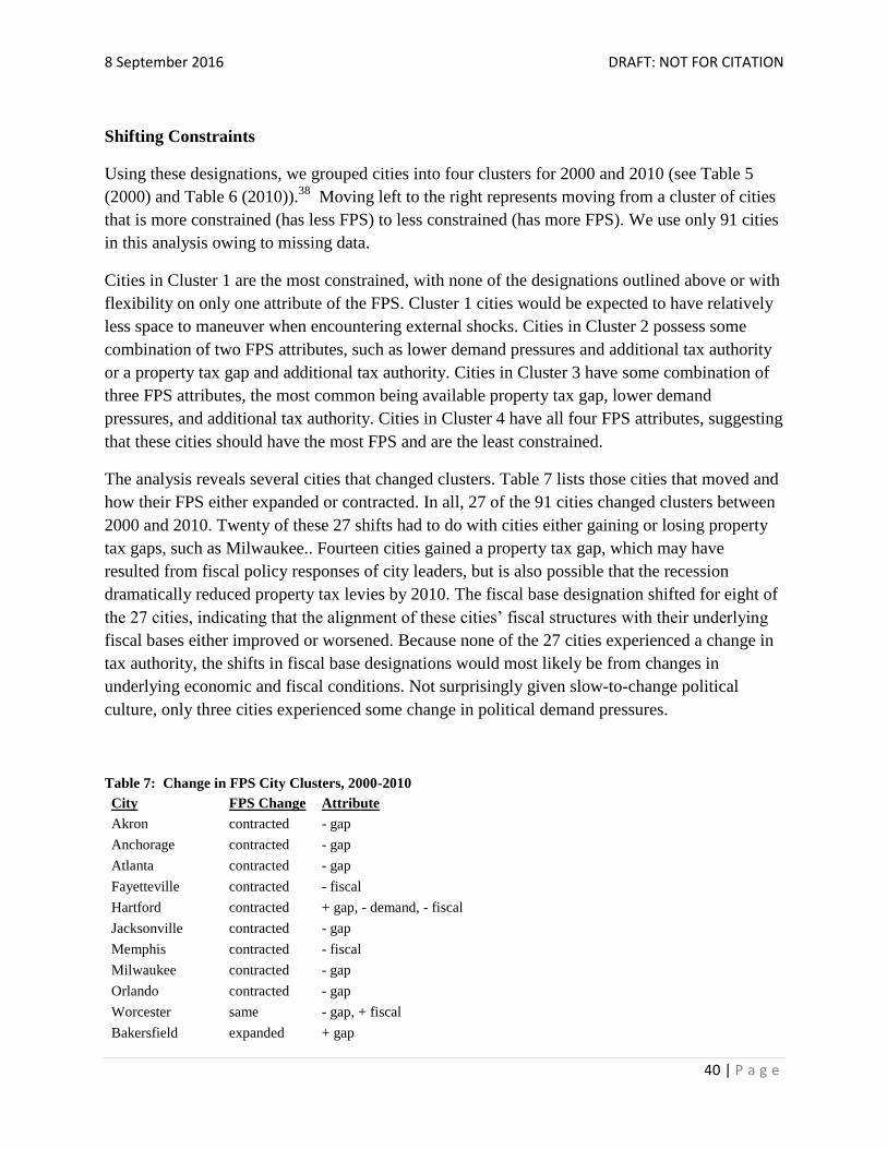
Shifting Constraints
Using these designations, we grouped cities into four clusters for 2000 and 2010 (see Table 5
(2000) and Table 6 (2010)).38
Moving left to the right represents moving from a cluster of cities
that is more constrained (has less FPS) to less constrained (has more FPS). We use only 91 cities
in this analysis owing to missing data.
Cities in Cluster 1 are the most constrained, with none of the designations outlined above or with
flexibility on only one attribute of the FPS. Cluster 1 cities would be expected to have relatively
less space to maneuver when encountering external shocks. Cities in Cluster 2 possess some
combination of two FPS attributes, such as lower demand pressures and additional tax authority
or a property tax gap and additional tax authority. Cities in Cluster 3 have some combination of
three FPS attributes, the most common being available property tax gap, lower demand
pressures, and additional tax authority. Cities in Cluster 4 have all four FPS attributes, suggesting
that these cities should have the most FPS and are the least constrained.
The analysis reveals several cities that changed clusters. Table 7 lists those cities that moved and
how their FPS either expanded or contracted. In all, 27 of the 91 cities changed clusters between
2000 and 2010. Twenty of these 27 shifts had to do with cities either gaining or losing property
tax gaps, such as Milwaukee.. Fourteen cities gained a property tax gap, which may have
resulted from fiscal policy responses of city leaders, but is also possible that the recession
dramatically reduced property tax levies by 2010. The fiscal base designation shifted for eight of
the 27 cities, indicating that the alignment of these cities’ fiscal structures with their underlying
fiscal bases either improved or worsened. Because none of the 27 cities experienced a change in
tax authority, the shifts in fiscal base designations would most likely be from changes in
underlying economic and fiscal conditions. Not surprisingly given slow-to-change political
culture, only three cities experienced some change in political demand pressures.
Table 7: Change in FPS City Clusters, 2000-2010
City FPS Change Attribute
Akron contracted - gap
Anchorage contracted - gap
Atlanta contracted - gap
Fayetteville contracted - fiscal
Hartford contracted + gap, - demand, - fiscal
Jacksonville contracted - gap
Memphis contracted - fiscal
Milwaukee contracted - gap
Orlando contracted - gap
Worcester same - gap, + fiscal
Bakersfield expanded + gap

8 September 2016 DRAFT: NOT FOR CITATION
41 | P a g e
Boise expanded + gap
Bridgeport expanded + fiscal
Cincinnati expanded + gap
Colorado Springs expanded + gap
Columbus expanded + demand
Dallas expanded + fiscal
Dayton expanded + demand
Las Vegas expanded + gap
Pittsburgh expanded + gap
Reno expanded + gap
Riverside expanded + gap
Sacramento expanded + gap
San Diego expanded + gap, + fiscal
Santa Rosa expanded + gap, + fiscal
Spokane expanded + demand
Stockton expanded + gap
Wichita expanded + gap
City Fiscal Responses from 2007 to 2012
We are particularly interested in how cities responded to the Great Recession, particularly
between 2007 and 2012. Despite some variation in the specific actions taken by cities, common
responses emerged. Generally, when cities confront declining economic and fiscal conditions,
they can raise additional revenue (from taxes, fees and charges, and intergovernmental
revenues), reduce expenditures by cutting programs and services (including staffing), or draw
down reserves. We examined city responses in these categories during the period using the 2010
city cluster designations.
Revenue Patterns—Overall, total city revenue declined across all clusters (see Figure
12). The largest drop occurred in Cluster 1 cities, those cities with the most constrained FPS. The
mean decline for total revenue was $186 per capita between 2007 and 2012.39
In all four clusters,
revenue declines were notable for non-tax revenue, with the scale of the decline following a
linear pattern. The largest drop occurred in Cluster 1 ($172 per capita), followed by Cluster 2 and
Cluster 3, and finally Cluster 4 ($52 per capita).
For nontax revenue, the largest source of revenue is intergovernmental, where there is notable
variation across the city clusters. Cities in Cluster 1 lost the largest amount, dropping by $103
per capita. Several cities in Cluster 1 are driving this decline, including Philadelphia (-$311),
Boston (-$318), and Providence (-$523). Here again, revenue declines follow a linear pattern
8 September 2016 DRAFT: NOT FOR CITATION
42 | P a g e
across the city clusters. (Cities in Cluster 4 experienced a mean increase of $17 per capita over
the period.)
Cluster 1 declines appear to be driven, in part, by the prevalence of cities in this cluster with
dependent schools (where school districts are the responsibility of city governments). Eight of
the 18 Cluster 1 cities have dependent schools. For these cities, funding for education comes
from a combination of local property tax revenues (typically a larger share than cities receive in
other states) and state assistance (which is provided to separate school districts in other states).
As a result, these cities receive a larger share of their annual revenues from the state and,
therefore, are likely to experience larger swings in intergovernmental revenues as economic and
fiscal conditions shift in similar ways for city and state governments. Overall, this pronounced
pattern in intergovernmental revenue changes matches up with expectations about the interaction
of cities’ FPS and their fiscal policy responses, showing that the more constrained cities
experienced more substantial revenue declines and the less constrained cities experienced
smaller declines or actual gains.
Patterns in tax revenue follow a somewhat similar, if less pronounced, pattern. Cities in Clusters
3 and 4 experienced the largest drops in tax revenues at $61 per capita and $60 per capita,
respectively. Several cities in these clusters experienced particularly large declines in tax
revenues: Tampa, FL (-$223 per capita); Richmond, VA (-$232 per capita); Virginia Beach, VA
(-$334 per capita); and Cape Coral, FL (-$416 per capita). For example, Tampa (Cluster 3),
characterized by lower demand pressures, available property tax gap, and better fiscal base
alignment, also relies more on local property tax revenue because it lacks additional sales or
income tax authority. The Great Recession, driven in large part by a decline in housing values
and wealth, significantly reduced local property tax revenue from $187.1 million to $119.4
million over the period. Many of the cities in Clusters 3 and 4 (33 of 41 cities) have authority
over two sources of local tax authority, in most cases a combination of a local property tax and
local sales tax. The Great Recession reduced both sources of revenue in most cases.
In comparison, cities with more constrained FPS experienced smaller tax revenue declines. Cities
in Cluster 1 experienced only $14 per capita declines. Cities in Cluster 2 experienced a slight
increase in tax revenue of $4 per capita. Although the pattern of tax revenue is not as linear as
non-tax revenues (and intergovernmental revenue in particular), those cities with more fiscal
policy space—presumably those cities more able to shape their tax revenue—experienced larger
declines in tax revenue during the period than more constrained cities.
The breadth of tax revenues affected and the size of their declines during the recession suggest
that tax revenue declines should have been significant for most cities. However, there was
surprising variation among cities, particularly in terms of the effect on local property tax
revenue.40
Much of that variation reflects the dramatically different housing markets and,
therefore, local property tax collections. The factors driving that variation likely have less to do

8 September 2016 DRAFT: NOT FOR CITATION
43 | P a g e
with the FPS of cities than other issues particular to the Great Recession and specific types of
housing markets.
In summary, non-tax revenue, and intergovernmental revenues in particular, declined for cities in
all four clusters during the timespan, but to a greater degree in cities with more constrained FPS
(cities in Clusters 1 and 2). Cities with less constrained FPS (Clusters 3 and 4) were more likely
to experience some combination of decline in tax and non-tax revenue.
Source: Comprehensive Annual Financial Reports, downloaded via Electronic Municipal Market Access
Expenditure Patterns— As with the patterns in city revenue, patterns in city
expenditures (see Figure 13) from 2007 to 2012 reveal the effects of the economic downturn.
Cities’ spending declined in all the categories except debt service. However, spending on city
programs and services did not decline in proportion to the decline in city revenue, suggesting that
cities balanced their budgets during the period using additional options, most likely by using
reserves. We account for city reserves by measuring spending as a share of cities’ total general
expenditures, that is, their fund balance. We will address patterns in fund balances in the next
section, but it is clear at first glance that reduced fund balances were common to cities in all four
clusters.
The interaction between FPS and spending responses yields less discernible patterns than for
revenue (excluding fund balances). However, when observing spending in aggregate, and
-200
-150
-100
-50
0
50
Figure 12: Per Capita Revenue Change, 2007-2012 (Governmental Funds)
(2012 dollars)
Cluster 1 Cluster 2 Cluster 3 Cluster 4
8 September 2016 DRAFT: NOT FOR CITATION
44 | P a g e
factoring out a few city cases where expenditure declines are anomalies, we begin to observe
patterns that are more unique to the clusters.
In the spending category of “general government,” Cluster 3 had the largest decline. A few cities
are driving those averages. Atlanta and Chattanooga, for example, reduced government spending
by $253 and $166 per capita, respectively. Without those two cities, the decline in the mean for
Cluster 3 declines from $34 per capita to $22. This leaves the differences among the clusters
minor, at $11 per capita decline for cities in Cluster 1, $23 for cities in Cluster 2, and $15 for
cities in Cluster 4. That cities in all four clusters exhibited similar patterns in general government
spending is not surprising given that most cities cut general government spending (largely for
city administrative services) in response to economic and fiscal shocks.
Spending on public safety declined substantially in Cluster 3 cities. Atlanta reduced spending by
$198 per capita; Richmond, VA, by $138; and El Paso, TX, by $171. The mean decline is $31
per capita. Excluding those three cities, the average decline is $20 per capita. Similarly, in
Cluster 2, Bridgeport, CT, drove up the average with a $324 per capita increase in public safety
spending. Without Bridgeport, public safety spending in Cluster 2 actually decreased by $28 per
capita. Here again, removing the extreme cases reveals that changes in spending on public safety
were relatively consistent across the cluster.
Perhaps more notable is that the scale of the changes in public safety spending was not
particularly large in any of the clusters, given that public safety expenditures typically
encompass the largest category of city spending. In other words, few cities significantly cut
spending on public safety during the recession. This is not surprising, given the corresponding
increases in demand for those services during recessions, as well as contracts with public safety
employees and the optics and related political challenges that come with public safety cuts.
Public works spending declined in all clusters, with the largest decline in Cluster 3. When
factoring out Kansas City’s $500 per capita decline, Cluster 3 declined by only $24 per capita
instead of $53 per capita. Although public safety spending declines were somewhat similar
across the four clusters, spending declined more in cities with the most restricted FPS.
Overall city spending declined in all four clusters, with Cluster 3 leading way with the largest
reductions. Once again, a handful of cities drive the reductions, with five cities experiencing total
spending reductions of more than $450 per capita. Total spending reductions for the remaining
16 cities were $47, slightly more than the average decline of $43 for Cluster 4 cities. Patterns
were again linear, with the largest reduction in Cluster 1 (most constrained) and the smallest
reduction in Clusters 3 and 4. In other words, the more constrained cities, with fewer tools at city
leaders’ disposal to respond to the recession, made greater cuts in city spending across the board.
City leaders in cities with more fiscal policy space to maneuver were able to avoid these more
drastic cuts.
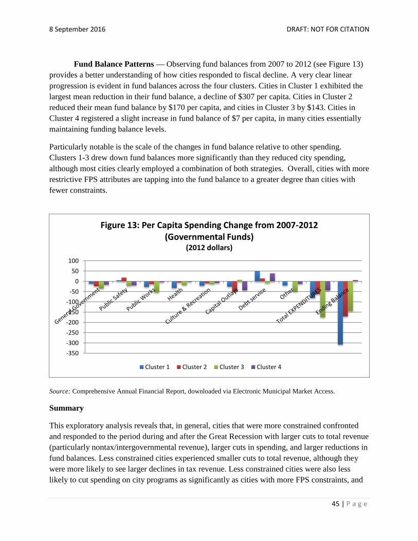
8 September 2016 DRAFT: NOT FOR CITATION
45 | P a g e
Fund Balance Patterns — Observing fund balances from 2007 to 2012 (see Figure 13)
provides a better understanding of how cities responded to fiscal decline. A very clear linear
progression is evident in fund balances across the four clusters. Cities in Cluster 1 exhibited the
largest mean reduction in their fund balance, a decline of $307 per capita. Cities in Cluster 2
reduced their mean fund balance by $170 per capita, and cities in Cluster 3 by $143. Cities in
Cluster 4 registered a slight increase in fund balance of $7 per capita, in many cities essentially
maintaining funding balance levels.
Particularly notable is the scale of the changes in fund balance relative to other spending.
Clusters 1-3 drew down fund balances more significantly than they reduced city spending,
although most cities clearly employed a combination of both strategies. Overall, cities with more
restrictive FPS attributes are tapping into the fund balance to a greater degree than cities with
fewer constraints.
Source: Comprehensive Annual Financial Report, downloaded via Electronic Municipal Market Access.
Summary
This exploratory analysis reveals that, in general, cities that were more constrained confronted
and responded to the period during and after the Great Recession with larger cuts to total revenue
(particularly nontax/intergovernmental revenue), larger cuts in spending, and larger reductions in
fund balances. Less constrained cities experienced smaller cuts to total revenue, although they
were more likely to see larger declines in tax revenue. Less constrained cities were also less
likely to cut spending on city programs as significantly as cities with more FPS constraints, and
-350
-300
-250
-200
-150
-100
-50
0
50
100
Figure 13: Per Capita Spending Change from 2007-2012 (Governmental Funds)
(2012 dollars)
Cluster 1 Cluster 2 Cluster 3 Cluster 4
8 September 2016 DRAFT: NOT FOR CITATION
46 | P a g e
they were able to maintain or only marginally draw down fund balances. Although the analysis
covers only one time period, it points to a clear relationship between the constraints on the fiscal
policy space of cities—the room for city leaders to maneuver when confronted by changing
conditions—and the resulting fiscal actions and outcomes of cities.
The FPS is a behavioral frame and needs to be better understood in order to (i) analyze the
efficacy of fiscal policy decisions, (ii) design federal or state programs, and (iii) identify
appropriate changes in those constraints that enhance city autonomy to efficiently, effectively
and fairly pursue their own pathways to make better communities and cities.
NOTES
1 This effort draws on the work we’ve done together, what we’ve learned, and our continuing commitment to
better informing the dialogue about cities. It also draws upon the interest of – and collaboration with – the Federal Reserve Bank of Chicago and the State-Local Fiscal Policy Working Group of the Fed banks, and the MacArthur Foundation’s interest in improving outcomes in the state-local arena. We are grateful to the participants of two Thinkers’ Sessions who helped shape the project and clarify the concept of Fiscal Policy Space. The Thinkers’ Sessions, supported by the Lincoln Institute of Land Policy, were convened in the Great Cities Institute of the University of Illinois at Chicago in March 2006 and January 2007. The participants included: Richard Feiock, Elisabeth Gerber, Deborah Carroll, Katherine Barrett, Richard Greene, Rachel Weber, Nathan Anderson, Rebecca Hendrick, William Barnes, Benoy Jacob, Kseniya Khovanova, Kim Rueben, John Petersen, David Garrison, Annette Steinacker, Joan Youngman, Brian Murphy, Daphne Kenyon, Jane Malme, David Perry, and Semida Munteanu. The FPS research team includes the co-Principal Investigators of the FPS project, Michael A. Pagano and Christopher Hoene, in addition to Yonghong Wu, Darrene Hackler, Paul Lewis, Richard Mattoon, Christiana McFarland and numerous graduate research assistants, including Shu Wang, Ayman Bari, Yu Shi, Nisa Yazici, Jill Mason Terzakis, James Eisenhauer, Samuel Bassett, Kathryn Cowlin, and Suriya Sundararaj. 2 See, e.g., Edward Glaeser, Triumph of the City: How Our Greatest Invention Makes US Richer, Smarter, Greener,
Healthier, and Happier (New York: Penguin Books, 2012); Bruce Katz and Jennifer Bradley, The Metropolitan Revolution: How Cities and Metros Are Fixing Our Broken Politics and Fragile Economy (Washington, DC: Brookings Institution, 2013). 3 Duranton and Puga argue that there still are gaps in understanding city growth: “Furthermore, some potential
drivers of the growth of cities are yet to be explored. The biggest gap is arguably studying the effects of municipal and city governments, local policies and public finance.” (p. 57) See Gilles Duranton and Diego Puga, “The Growth of Cities.” CEPR Discussion Paper no. DP9590. (August 2013), http://ssrn.com/abstract=2309234. 4 Lindsay Holst, “The Precision Medicine Initiative: Data-Driven Treatments as Unique as Your Own Body,” White
House Briefing Room, January 30, 2015, https://www.whitehouse.gov/blog/2015/01/30/precision-medicine-initiative-data-driven-treatments-unique-your-own-body. 5 The Great Depression witnessed unemployment rates of nearly 25 percent, while the Great Recession’s
unemployment rate reached nearly 10 percent by 2009. The stock market (Dow Jones Industrial Averages) dropped by 89 percent by 1933, but only 20-30 percent by 2010. Price declines were nearly 25 percent during the Great Depression, while they remained steady during the Great Recession. Bank foreclosures reached nearly 50 percent in 1933, but only 10 percent during the Great Depression. Social disruptions were fairly limited during the Great Recession but widespread during the 1930s. See, e.g., Michael A. Pagano, “Cities and the Great Recession: Lessons in Dynamic Change and Adaptation.” In Metropolitan Resilience in a Time of Economic Turmoil, ed. M. A. Pagano (Urbana: University of Illinois Press, 2014), 3-18.

8 September 2016 DRAFT: NOT FOR CITATION
47 | P a g e
6 Christiana McFarland and Michael A. Pagano, City Fiscal Conditions in 2015 (Washington, DC: National League of
Cities, 2015). 7 According to the latest census estimates, 38 percent of total own-source revenues are derived from user fees,
charges, and miscellaneous, while 28 percent is derived from the property tax and 26 percent from both the local-option sales and income taxes. 8 McFarland and Pagano, City Fiscal Conditions in 2015.
9 According to Bureau of Labor Statistics, seasonally unadjusted data released for April 2016, the total number of
local government employees is 14,463,000, as compared with 14,914,000 employees for November 2008. This represents an improvement over 2013’s low-water mark, which counted a half-million fewer local government positions than in 2008. http://www.bls.gov/web/empsit/ceseeb1b.htm 10
Studies on city fiscal conditions are abundant in the academic literature. Our argument is not that there’s a dearth of studies, rather that these studies focus on the ‘average’ city without recognizing the enormous variation among city fiscal options or they ignore the fiscal policy behavior of cities or the constraints within which fiscal decision making occurs. Examples of a city fiscal conditions studies include: Ladd, H. F., and Yinger, J.M. 1989. America’s Ailing Cities: Fiscal Health and Design of Urban Policy. Baltimore, MD: John Hopkins University Press; Tannenwald, Robert. 1999. “Fiscal disparities among the states revisited.” New England Economic Review: 3-25; Advisory Commission on Intergovernmental Relations. 1981. Measuring the fiscal capacity and effort of state and local areas. Washington, DC: ACIR; Clark, T.N. and Ferguson, L.C. 1983. City Money: Political Processes, Fiscal Strain and Retrenchment. New York: Columbia University Press; Hendrick, R. 2004. “Assessing and measuring the fiscal health of local governments: Focus on Chicago suburban municipalities.” Urban Affairs Review, 40 (1): 78-114; Chernick, Howard, Adam H. Langley, and Andrew Reschovsky. 2015. “Comparing central city finances using Fiscally Standardized Cities.” Journal of Comparative Policy Analysis 17(4): 430-440; Hendrick, R. 2014. “Municipal fiscal policy space and fiscal structure: Tools for managing spending volatility.” Public Budgeting and Finance, 34 (3): 24-50. 11
Michael A. Pagano and Christopher W. Hoene, “States and the Fiscal Policy Space of Cities.” In The Property Tax and Local Autonomy, Michael Bell et al., eds. (Cambridge, MA: Lincoln Institute of Land Policy, 2010). 12
By representative, we mean that the cities selected should represent a sizeable portion of the municipal sector in terms of economic output and fiscal capacity. The sample must also provide sufficient variation along several dimensions, including revenue structures (tax authority) and region of the country (using U.S. Census regions and Federal Reserve districts). Therefore, the selected project cities do not represent a random sample of cities. The sample also reflects a focus on feasibility in terms of data collection, including cities whose economic and fiscal information is regularly reported in national data sources or that are willing to provide requested information and data. A key challenge in selecting a sample of cities that is economically representative of the municipal sector is that economic output data are not collected regularly for a wide range of cities. For example, Gross Domestic Product estimates are typically available for metropolitan areas, but not as readily or regularly available for individual cities. As a result, the project team employed a selection method that attempts to crudely approximate the relative economic and fiscal importance of large cities within metropolitan areas. Project cities were selected based on their relative population size and the relative population size of their metropolitan statistical area (MSA), based on the 2011 U.S. In order to be included in the sample, a city must be among the largest central cities in the U.S. and within the largest MSA’s in the U.S. For example, a smaller central city located in large MSA might not be included in the sample, or a larger central city located in a smaller MSA might not be included. The interaction of city size and MSA size produced a list of cities that approximates the most economically and fiscally influential cities in the U.S. Washington, D.C. is excluded from the sample because of its unique governmental structure. In addition, the analyses conducted as part of the FPS project will occasionally separate out or exclude New York City when the relative fiscal capacity would otherwise overwhelm aggregated city data. 13
We use the terms “cities” and “municipalities” broadly to refer to all municipal governments. 14
These states include Alaska, Connecticut, Maine, Maryland, Massachusetts, Michigan, New Hampshire, New Jersey, New York, Rhode Island, Tennessee, and Virginia.
8 September 2016 DRAFT: NOT FOR CITATION
48 | P a g e
15
Local income taxes, as we refer to them here, are not always referred to as income taxes by the individual states. In Kentucky, for instance, cities and counties levy two income related taxes, an occupational license tax on income earned in a jurisdiction by individuals and a net profits tax on businesses. 16
Oklahoma cities can levy a property tax for debt service. 17
“General revenue” as defined by the U.S. Census of Governments, including all local revenues except revenues from utilities and liquor store operations. This definition is broader than how states and cities budget, in which the “general fund” is the annual operating budget, with a series of other funds for special activities/projects. 18
Our measure of own-source revenue reliance differs from a commonly used census definition of “own-source revenues” in that local revenues are not counted as own source if there is no local authority (using our definition of authority based on a local option that can be used for general purposes). Local fees and charges revenues include administrative and court fees, waste disposal fees, building permits, development impact fees, law enforcement and fines and fees, and service fees for libraries and parks. 19
Measured as one standard deviation above the mean capacity (percent share of general revenue). Throughout the report we generally use the mean and standard deviation statistics to determine break points for differences among states. 20
We created a five-point scale to indicate the restrictiveness of TELs in 2012. A higher number indicates more restrictive TELs and therefore the less space for fiscal policies. The scale is: 1 = no TELs; 2 = nonbinding property tax limit; 3= potential binding property tax limit; 4 = nonbinding property tax with general revenue or expenditure limit, potential binding property tax limit with general revenue or expenditure limit, or binding property tax limit; and, 5 = binding property tax with general revenue or expenditure limit . For the purpose of analysis, we reverse the scale so that a lower number indicates less fiscal policy space, a direction that is consistent with the other dimensions in our analysis. We place cities along an axis based on this five-point scale. Here again we examine the three major sources of state and local tax revenue, the property tax, sales tax, and income tax. Once again, we rate municipalities as having authority if they have a local option to control the tax rate and if the revenues are for general use. We also define tax authority as one that has been executed, rather than one that is authorized by legislation and not implemented. We use data collected from US Census of Governments (2012) and official websites of city governments to determine whether the cities in our sample have authority to levy a property tax, sales tax, and income tax. This less (or non-) binding / potential binding approach is well documented within the academic and analytic research on TELs. For instance, see Daniel R. Mullins and Bruce A. Wallins. 2004. “Tax and expenditure limits: Introduction and overview.” Public Budgeting and Finance 24: 2–15. 21
Georgia had a potentially binding property tax limit that expired in 2011. 22
For state-imposed TELS, we used Lexis Legal to identify laws on state-imposed TELs. We cross-referenced our list of laws with secondary data sources such as Advisory Commission on Intergovernmental Relations, Tax and expenditure limits on local governments. Report M-194. (Washington, DC: Government Printing Office, 1995) and Lincoln Institute of Land Policy. We also used a search of legislative session laws to track TEL amendments, producing a panel data set on TEL changes. We used the following protocol to code TEL terms and conditions: limit types, maximum allowable rates for growth, institutional codification (constitutional vs. statutory), override processes, and TEL exemption. For a detailed discussion and explanation, see Shu Wang, Effects of State-Imposed Tax and Expenditure Limitation on Municipal Revenue Structure: A Legal Approach, PhD dissertation, Department of Public Administration University of Illinois at Chicago, 2015. For locally imposed TELS, we used Brooks and Phillips’ survey responses as a guide in identifying which cities may have TELs. We then attempted to confirm legislation in city charters and municipal codes. We collected the local ordinances and coded the limit rates specified, the tax base on which the rate is applied, whether the limit is binding, whether the referendum is allowed to override the limits, and whether supermajority is needed for tax increase. See, Leah Brooks and Justin Phillips, “When and why do cities bind themselves? The existence and extent of locally imposed tax and expenditure limits.” Working Paper. Cambridge, MA: Lincoln Institute of Land Policy, 2009. 23
The data are limited in the following ways. First, some cities do not report assessed values for a particular year or throughout the entire study period, which reduced the number of observations from 1,700 to 1,609. Second, there are many instances of a negative TEL gap. Negative values indicate that the cities managed to exceed the legal TEL
8 September 2016 DRAFT: NOT FOR CITATION
49 | P a g e
ceiling through exemptions or voter overrides. Because of the lack of data on the amount of TEL exemptions, we are unable to incorporate the TEL exemptions into the TEL gap measure. 24
They are Fort Wayne, IN; Indianapolis, IN; Huntsville, AL; Birmingham, AL; Philadelphia, PA; Pittsburgh, PA; Minneapolis, MN; Shreveport, LA; Chicago, IL; Des Moines, IA; Detroit, MI; and Little Rock, AR. Although there is a levy limit imposed by Pennsylvania, the limit only applies to cities with population less than 250,000, and thus is not applicable to Philadelphia and Pittsburgh. 25
For cities that are authorized to collect income tax from commuters, we use per capita income for the entire metropolitan areas to incorporate the exported portion of income tax to nonresidents. 26
The ideology variable is a result of two larger efforts. First, we utilize Tausanovitch and Warshaw to estimate mrp_ideology, where the estimate of left/right ideology of city residents is on a standardized scale, where negative values represent liberalism and positive values conservatism. Tausanovitch and Warshaw estimated from pooled surveys of 275,000 Americans, using multilevel regression and post-stratification (MRP) to impute the “ideal points” of public opinion at the city level for cities of 25,000 or higher population. Because Tausanovitch and Warshaw state that these estimates represent the average value for each city from 2000 to 2011, we interpret these values as approximating 2006 or 2007 values, thus are appropriate for the 2007 FPS sample year. For other FPS years, we simulate MRP ideology scores using our second procedure to estimate the “ideology_##_sim” variables. The resulting ideology values for each city are estimated (or simulated) values of mrp_ideology_Tausanovitch for the sample years of the Fiscal Policy Space Project: 1992, 1997, 2002, 2007, and 2012. Since the Tausanovitch & Warshaw ideology estimate was available only for a single time point, taken to be 2006, we adjusted the ideology scores to the FPS years by using presidential vote variables, which are available for presidential‐election years, but only at the county level. To make these ideology estimates, we used the following procedure. First, we ran an OLS regression of mrp_ideology_Tausanovitch on elec_06interp (the latter being the average of the presidential vote in 2004 and 2008). The residuals of this regression provide a good way to “correct” the presidential‐election variables (given they are measured at the county rather than municipal level) and relate them to the MRP values. By construction, a regression of mrp_ideology_Tausanovitch on elec_06interp and the residuals of the previous regression fits the data perfectly (i.e., R‐squared of 1.0). We use the values of the coefficients and constant of this regression equation in order to estimate values of ideology for earlier and later years in the data series. Specifically, the equation is: ideology_##_sim = .8096758 – (.0190509 * elec_##) + residMRPelec06, where ## is the 2‐digit year abbreviation, and residMRPelec06 are the residuals of the regression of mrp_ideology_Tausanovitch on elec_06interp (and * is a multiplication sign). We use the following presidential election variables for specific years of ideology:
ideology_92_sim: elec_92
ideology_97_sim: elec_96
ideology_02_sim: elec_02_interp
ideology_07_sim: Here we simply substitute the mrp_ideology_Tausanovitch value, which
should correspond to approximately 2006.
ideology_12_sim: elec_12 Special note regarding Anchorage, AK: Presidential election data are missing for Anchorage. However, Tausanovitch and Warshaw did provide an ideology estimate for Anchorage. In order to not lose a case from the analysis, we have inserted values of ideology_##_sim for Anchorage for the missing years (i.e., other than 2007). We do this by adjusting upward and downward its mrp_ideology_Tausanovitch value by the average difference from 2007 to the year in question among the other 99 FPS cities. Source: Downloaded and entered from http://www.americanideologyproject.com/ , “City‐Level Public Preference Estimates”; for documentation of the method, see Chris Tausanovitch and Christopher Warshaw “Measuring Constituent Policy Preferences in Congress, State Legislatures, and Cities,” Journal of Politics 75(2)(2013): 330‐342. 27
Deacon, R. T. (1978). “A demand model for the local public sector,” Review of Economics and Statistics 6, 184‐92. 28
The rent-to-income ratios differ due to data availability. For rentincomeratio_00 and rentincomeratio_10,we use a ratio of annualized rent of the given Census year (for example 2000) to median household income the year prior (for example 1999) because the decennial Census asks respondents for their income in the prior calendar year. The rent-to-income ratio is a measure of the unaffordability of rental housing in the city. The year 2010 is used instead

8 September 2016 DRAFT: NOT FOR CITATION
50 | P a g e
of 2012 because lack of data after 2010 makes it impossible to align a straight‐line interpolation of the value of the rent‐to-income ratio for census year 2010 with FPS sample year 2012. Thus, the 2010 data are used for the 2012 analysis. 29
Paul G. Lewis and Max Neiman. 2009. Custodians of place: Governing the growth and development of cities. Washington: Georgetown University Press. 30
The rent-to-income ratios shown differ due to data availability. For rentincomeratio_00 and rentincomeratio_10: Ratio of annualized rent (in the given Census year, for example 2000) to median household income the year prior (for example 1999; note that the decennial Census asks respondents for their income in the prior calendar year). This is a measure of the unaffordability of rental housing in the city. The year 2010 is used instead of 2012 for this variable due to the fact that a straight‐line interpolation of the value of the rent‐to-income ratio for the Census year 2010 to coincide with FPS sample year 2012 is not possible because of a lack of data subsequent to 2010; thus the 2010 data is used for 2012 analysis. 31
The municipal‐level data are unavailable, and Anchorage, AK, and Lincoln, NE, are missing from the source data for the final two years (2007, 2012). For documentation, see http://unionstats.gsu.edu and Barry T. Hirsch and David A. MacPherson, "Union Membership and Coverage Database from the Current Population Survey: Note," Industrial and Labor Relations Review, 56 (2)( January 2003):349‐54. 32
The demand scale is constructed by standardizing the values of the three individual items to mean 0 and variance 1, and then summing the standardized values. Note that the Ideology variable, which runs from liberal (low values) to conservative (high values), is reversed before the standardizing and summing takes place. The command in the Stata 12 statistical package that produces the scale is: alpha ideology_##_sim union##_coverage rentincomeratio_##, std gen(demand_scale_##); where ## is the 2‐digit year (02 or 12), and italicized words are variable names. Alpha reliability coefficient for the scale is .73 in 2002. Note that demand_scale_12 is a summary scale of our estimate of the political pressure for fiscally expansionary policy in each city in 2012. This variable is constructed exactly like the demand scale for the earlier 13 years, except that we use rentincomeratio_10, given that we lack estimates of median rent or median income after 2010. The alpha reliability coefficient for demand_scale_12 is .70. 33
Sarah Emmans, “Providence Case Study,” unpublished report for the George Mason University Municipal Sustainability Project, Center for State and Local Government Leadership, George Mason University, http://s3.amazonaws.com/chssweb/documents/12790/original/GMU_Providence_9.13.pdf?1379560620. 34
Ibid. 35
Ibid. 36
Denise Dowling, “Cease Fire,” Rhode Island Monthly, May 2010. http://www.rimonthly.com/Rhode-Island-Monthly/May-2010/Cease-Fire/index.php?cparticle=3&siarticle=2#artanc. 37
We first calculated Z-scores for the fiscal base and the demand pressure variables to determine if a city’s score was above or below the mean of each of these variables. We further classified cities by whether they have access to more than a local property tax (either a local sales or income tax) and if cities have a property tax gap, if they have room to increase their revenues through the property tax (despite the existence of TELs). 38
The biggest challenge in clustering cities is to demarcate the clusters clearly; that is, how to determine the threshold that places cities in each cluster. Our strategy centered on the mean for the demand pressure and fiscal base attributes of the FPS. We then categorized cities by whether they had access to more than a property tax and whether they had a property tax gap and could increase the levy. Clustering cities on the basis of whether they are above or below a mean value has its flaws, but for our purposes of understanding city fiscal behavior, this method allows us to compare and analyze similarly situated cities within the FPS framework. Further and more robust testing of this relationship is needed to truly understand the subtle differences between cities and how the constraints they confront drive their responses to changing economic and fiscal conditions. 39
All revenue and expenditure data are standardized to 2012 dollars and presented in per capita terms. Revenue and expenditure data were collected from the city Comprehensive Annual Financial Reports posted on the Electronic Municipal Market Access (EMMA) website. See the description of data extraction for the FPS project at: http://www.srl.uic.edu/fiscalpolicyspace/index.php 40
See, for example, the National League of Cities’ annual reports on “City Fiscal Conditions” 2009-2012.