The Fiscal Effects of Population Aging in the U.S ... · Our analysis here has two goals: ... whose lives were saved by declining mortality might be functionally ... The Fiscal Effects

This PDF is a selection from a published volumefrom the National Bureau of Economic Research

Volume Title: Tax Policy and the Economy, Volume16

Volume Author/Editor: James M. Poterba, editor

Volume Publisher: MIT Press

Volume ISBN: 0-262-16210-5

Volume URL: http://www.nber.org/books/pote02-1

Conference Date: October 30, 2001

Publication Date: January 2002

Title: The Fiscal Effects of Population Aging in theU.S.: Assessing the Uncertainties

Author: Ronald Lee, Ryan Edwards

URL: http://www.nber.org/chapters/c10865

THE FISCAL EFFECTS OFPOPULATION AGING INTHE U.S.: ASSESSING THEUNCERTAINTIES

Ronald Lee and Ryan EdwardsUniversity of California

EXECUTIVE SUMMARY

Population aging, accelerating as the Baby Boom generations age, willhave important fiscal consequences because expenditures on social secu-rity, Medicare, and institutional Medicaid make up more than a third ofthe federal budget. However, the projected fiscal pressures are far in thefuture, and long-term projections are very unreliable. Our analysis herehas two goals: to examine the fiscal impact of population aging, and to dothis in a probabilistic setting. We find that the old age dependency ratio isvirtually certain to rise by more than 50% through the 2030s, and willprobably continue to increase after 2050, possibly by a great deal. Undercurrent program structures, population aging would be virtually certainto increase the costliness of Federal programs as a share of GDP by 35percent (±2 percent) by the 2030s, and by 60 percent (± 15 percent) in thesecond half of the century. We project Federal expenditures (excludinginterest payments and pre-funded programs) to rise from 16 percent ofGDP in 2000 to 30 percent in 2075, almost doubling, while state and local

Research for this paper was funded by a grant from NIA, R37-AC11761. We thank TimothyMiller for his help with various parts of the analysis, and James Poterba for helpful com-ments.

142 Lee & Edwards

expenditures rise only modestly relative to GDP. Almost all of this in-crease is for programs going primarily to the elderly, which rise from 8percent of GDP in 1999 to 21 percent of GDP in 2075, due mainly to costs ofhealth care for the elderly, with pensions a distant second. We expect thatgovernments wifi respond to these aging-induced cost changes by alter-ing program structures, so that these conditional projections will not berealized. Looking at social security, we find that raising the payroll tax rateby 1.89 percent would have relatively little effect on the probabilities ofearly exhaustion, raising the 2.5 percent bound for the exhaustion datefrom 2024 to 2036, but raising the median date of exhaustion from 2036 to2070, and with a 55 percent chance of insolvency within the 75 yearhorizon. Looking at Medicare, which now costs 2.2 percent of GDP, weproject a median share in 2075 of 11 percent, five times as great, with a 95percent probability interval at 5 percent to 26 percent of GDP. Thus thereis a 97.5 percent chance that the ratio wifi at least double, and a 2.5 percentchance that it wifi increase at least twelve-fold. Although the future ishighly uncertain in many respects, unforeseen demographic or economicchange wifi almost certainly not avert the long-run fiscal crunch. Chang-ing demographic realities will require some combination of substantial taxincreases or substantial benefit cuts, or other forms of restructuring.

1. INTRODUCTIONExpenditures on social security, Medicare, and Medicaid for nursing-home care together make up more than a third of the federal budget.1These are all programs for the elderly, paid for largely out of taxes on theworking-age population. Around 2010, the Baby Boom generations willbegin to turn 65 and to draw on these programs, and by 2040, the ratio ofelderly people to those in the current working ages wifi have doubledfrom about 0.2 to about 0.4. Clearly, population aging will exert heavypressure on the federal budget in the coming decades. Nonetheless,there are many questions about this process. The projected fiscal pres-sures are far in the future, and long-term projections are very unreliable;might not the whole problem evaporate if we just wait? For example, wifiincreased costs in programs for the elderly be offset by decreased expendi-tures for children elsewhere in the federal budget and in the state andlocal budgets? Wifi the passing of the Baby Boom generations bring fiscalrelief? Wifi high-fertility immigrants raise national fertility, as Censusprojects? Or will fertility in the U.S. move towards low European levels,

1 Institutional Medicaid is the part of the Medicaid program that pays for nursing-homecare, primarily for the indigent elderly.

The Fiscal Effects of Population Aging in the U.S. 143

closer to one child per woman, greatly intensifying population aging? Inaddition to these demographic sources of uncertainty, there are verysubstantial economic uncertainties. These are well illustrated by the rapid-ity with which projections of fiscal doom in the mid-1990s were replacedin the late 1990s by projections of burgeoning surpluses, which haverecently been corrected to show declining surpluses over the short run.To formulate fiscally responsible policies, policymakers must have notonly best-guess forecasts of the future, but also a measure of the uncer-tainty surrounding these forecasts.

Before proceeding, some background will be helpful. First, it is impor-tant to put population trends in the U.S. into international perspective.Among the industrial nations, the U.S. has high fertility and a stingypublic pension system. Combined with middling mortality and immigra-tion, this adds up to relatively mild population aging and to relativelymodest fiscal pressure, compared to most European nations or Japan.An OECD study (Roseveare, Leibfritz, Fore, and Wurzel, 1996) foundthat the fiscal imbalance in the U.S. public pension system over the next75 years was among the smallest of any of the OECD countries, relativeto GDP. The fiscal consequences of population aging for the U.S. wifiindeed be severe, but in many other industrial nations they wifi besimply staggering.

Second, it is important to distinguish between the fundamental re-source problem posed by population aging, which would exist whateverour institutional structures, and the particular problems that arise specifi-cally because of our institutional arrangements for supporting the el-derly, including government programs.

Population aging raises the number of elderly people relative to thenumber of working-age people, when we hold the age boundary con-stant at some level such as age 65. In this sense, population aging occurspartly because individuals live longer, and partly because birth rates arelower, so that younger generations are smaller at birth than the oldergenerations. Longer life, by contrast, results at least in part from betterhealth, so that elderly people at any specific age are more vigorous andless likely to be disabled. For many years, it was feared that peoplewhose lives were saved by declining mortality might be functionallyimpaired by their close brush with death or by weaker constitutions, sothat disability rates at older ages would rise. In the U.S., at least, this hasnot happened, and indeed rates of disability at older ages are decliningat roughly the same rate as mortality itself. Older people wifi increas-ingly be functionally able to prolong their working lives (Manton,Corder, and Stallard, 1997; Freedman and Martin, 1999; Crimmins,Saito, and Ingegneri, 1997). People may choose to take their additional

144 Lee & Edwards

years of life as leisure years rather than as working years, and conse-quently they may need to save more or pay higher taxes to support thoseadditional years of leisure. That is a matter of choice, and not caused byaging itself. In this sense, longer life does not cause a fundamentalresource problem. By contrast, lower fertility means there are fewerworking-age people in the population relative to the elderly, withoutaltering the health or functional status of the elderly. Population agingdue to low fertility, unlike that due to low mortality, does fundamentallyalter the resource constraints facing society.

Population aging occurs in the context of a particular set of institutionsand traditions. In the U.S., the median age at retirement, far from risingwith increasing longevity, has declined by five years since 1950. To somedegree, this decline reflects a choice for more leisure at the end of life,influenced by higher lifetime incomes and the public and private pen-sions which have made it easier for people to realize what would anywayhave been their preferred life-cycle plans. That is the positive side of thestory. On the negative side, however, both public and private pensionprograms have incorporated incentives for earlier retirement, whether bydesign or by accident. In Europe, the easy availability of government-provided disability and unemployment benefits for older people hasadded to these incentives, and extended them to younger ages (Gruberand Wise, 1999). These pension, disability, and unemployment programscreate an implicit tax on continuation of work, inducing many people toretire early. When population aging occurs in the context of rigid anddistortionary institutions, particularly severe problems may arise. This isthe case for most public pension programs throughout the OECD coun-tries, and to a lesser extent for the U.S.

Institutional arrangements surrounding the provision of health care,particularly for the elderly, shape the impact of population aging onpublic health care costs. Once again, we must distinguish betweenlonger life and lower fertility as causes of population aging. Longer lifegoes with improved health in old age, and the net effect on health costsappears to be slight (Lubitz and Prihoba, 1984; Lubitz, Beebe, and Baker,1995). Nor have the costs of typical medical procedures risen in realterms, on the contrary, they may have fallen (Cutler, McClellan, New-house, and Remler, 1998; Cutler and Sheiner, 2000). Why, then, aregovernment health care expenditures projected to rise so strongly rela-tive to GDP over the twenty-first century? First, because lower fertilitywifi mean fewer workers to bear the cost of health care for the elderly(that is, future GDP will be lower than otherwise). Second, becausepopulations of industrial nations have a great appetite for the costly newprocedures made available by striking technological advances in medi-


cine over recent decades, advances which are expected to continue in thefuture. In the U.S., these two factorspopulation aging due to lowfertility and the purchase of costly new biomedical technologiesareexpected to account for roughly equal shares of the projected increasedexpenditure on health care relative to GDP (Lee and Miller, 2001b). Theportion of the increase due to low fertility and population aging cannotbe avoided, except possibly by pro-natalist and pro-immigration poli-cies. It is important to make sure that the other part, due to increasedquantity and quality of health care services consumed, is growing in away consistent with individual and social preferences, not simply be-cause of distortions arising from the structures of institutions formeddecades ago.

It is easy to exaggerate the fiscal pressures generated by populationaging. In practice, the structure and generosity of programs do not re-main fixed as population changes, and changing population age distribu-tions have only modest power to explain government expenditures onsocial welfare programs in the past. The structure and generosity ofprograms may be rigid in the short term, but in the longer term these tooadjust. We should keep in mind, however, that even if the fiscal pres-sures are mitigated by program changes, these mitigating changes maysimply pass costs on to the beneficiaries, in the form of later retirementor reduced medical benefits.

This paper will begin by discussing demographic change in the U.S.Next, it wifi discuss approaches to assessing the uncertainty of projec-tions, which is then followed by an overview of our own probabilisticprojections of population aging. Then it wifi consider how populationaging alters the budgetary trade-offs that constrain government pro-grams in the aggregate, contingent on the continuation of current pro-gram structure. An overview of stochastic budget projection techniquesfollows, motivated by a summary of deterministic predictions. The pa-per will then discuss in more detail the uncertainty of projections forsocial security and for Medicare. In the final section, we discuss ourresults.

2. POPULATION CHANGE IN THE U.S.2.1 FertilityOver the past two centuries in the U.S., the economic roles of women andchildren have changed, incomes have risen dramatically, mortality hasdeclined, the frontier has been settled, and contraceptive technologyhas advanced. Consequently, fertility has declined steadily from 7 or 8births per woman in 1800 to 2.0 births per woman today, a decline

146 Lee & Edwards

interrupted by the Baby Boom between 1946 and 1965. Similar factorshave led to a fertility decline in other industrial countries as well. How-ever, fertility in the U.S. has always been high compared to levels in otherindustrial populations. The average level for Europeanpopulations is 1.4births per woman, with some countries like Spain, Italy, and Germanyclose to 1.2, and a few smaller populations close to 1.0. Will fertility in theU.S. decline toward European levels in the coming decades? Two consid-erations reduce the likelihood. First, European women typically report onsurveys that they would like to have 2 children on average, suggestingthat fertility may rise in the future. Second, the average age of childbear-ing has been rising steadily in most European countries in recent de-cades, as women postpone giving birth. This trend distorts the standardfertility measure downward by 0.2 to 0.4 births, relative to fertility levelsover the life cycle of these women, again suggesting that European fertil-ity may rise in the future.

Fertility is high in the U.S. in part due to the higher fertility of minoritygroups such as African Americans, Latinos, and Asians. Projectionsindicate that the population share of non-Hispanic Whites wifi declinefrom around 70 percent today to around 50 percent by 2050. Will grow-ing population shares of these minority groups lead to higher aggregatefertility? The U.S. Census Bureau has assumed in its recent projectionsthat it will. We are skeptical. It is mainly first-generation immigrantswho have high fertility; by the third generation fertility has historicallyconverged to the levels of the general population (Smith and Edmons-ton, 1997). For example, first-generation Latino women have more thanthree births on average, whereas third-generation Latino women haveonly two. Furthermore, fertility in the sending countries in Latin Amer-ica and East Asia is rapidly falling In Mexico, fertility is now down to 2.6births per woman and falling rapidly, while many populations in EastAsia, including China, have fertility below replacement level. This sug-gests that future immigrants will not have fertility that is much higherthan the rest of the U.S. population.

Overall, therefore, we believe it is reasonable to project, as a pointestimate, that fertility levels continue at the current level of about 2.0,while noting that there is a great deal of uncertainty about this centralforecast.

2.2 MortalitjImprovements in nutrition, public sanitation and hygiene, personal hab-its, biomedical technology, and health service delivery have caused mor-tality declines throughout the world. Dramatic progress first againstinfectious disease, and then against chronic and degenerative disease,


has brought life expectancy in most industrial nations from 30 to 40 yearsat birth in the early nineteenth century to 75 to 80 years at birth today.The acceleration of the rate of decline in death rates at the older ages,even above 100, in recent decades has been particularly striking (Kan-nisto, Lauritsen, Thatcher, and Vaupel, 1994). Mortality is expected tocontinue to decline in the twenty-first century, but how far and how fastis open to question and controversy. The pessimists believe that it will bedifficult to raise life expectancy above 85 years without truly revolution-ary medical advances to slow the progress of aging itself (Fries, 1980,1984; Olshansky, Carnes, and Desesquelles, 2001; Board of Trustees,2001). Optimists believe that advances in stem-cell and genetic therapiesmay raise life expectancy as high as 150 years in this century. Forecastingmethods based on long-run trend extrapolation suggest that life expec-tancy in the U.S. wifi rise from its current 76.7 years to around 86 yearsby 2075, plus or minus 4 years (Lee and Carter, 1992; Lee and Miller,2001a; Tuljapurkar, Li, and Boe, 2000). Our forecasts in this paper wifi bebased on this latter approach.

2.3 ImmigrationThe annual number of net immigrants to the U.S. has risen linearly since1950, and shows no signs of decelerating in recent years. Nonetheless,because immigration is a policy variable, we have elected to follow theSocial Security Actuaries in assuming that the net annual number willremain at 900,000. Certainly a case could be made for forecasting thelinear trend to continue.

2.4 Projections by the U.S. Bureau of the Census and the SocialSecurity AdministrationWhile the assumptions about net immigration are very similar betweenCensus and SSA, the assumptions for fertility and mortality are quitedifferent. The SSA assumes that fertility will decline from about 2.05children per woman today to 1.95 by 2025, remaining constant thereafter.The USBC assumes that fertility will instead increase from its currentlevel to 2.22 in 2050, then declining slightly to 2.20 in 2075. The differenceof about 0.25 in fertility implies an eventual difference of about 0.5 per-cent per year in the population growth rate, which is substantial. Further-more, the SSA assumes a slower increase in life expectancy, to 81.7 in2050 and 83.0 in 2075, vs. 84.0 and 87.1 for the USBC. Thus by 2075,Census has life expectancy higher by four years than the Actuaries. Thesedifferences in fertility and assumed mortality decline lead Census to pre-dict more rapid population growth, and indeed, while the SSA projectsgrowth at 0.3 percent per year in 2050 and 2075, Census projects 0.7

148 Lee & Edwards

percent per year in both years, more than twice as rapid. By 2075, thepopulation projected by Census is 80 million greater than that by the SSA.Higher fertility eventually makes a population younger, while higher lifeexpectancy makes it older, so the differences in the projected old agedependency ratio (OADR) are not as great as otherwise. In 2050, the SSAOADR is lower, and in 2075, the Census OADR is lower.

2.5 Population ProjectionsBased on this discussion of fertility, mortality, and immigration, it isstraightforward to carry out the arithmetic of a population projection,generating forecasts for total population size and age distributions fromwhich measures such as the OADR could be calculated. Before doingthis, however, we wifi pause to consider how much confidence shouldbe put in results of this sort.

3. THE UNCERTAINTY OF PROJECTIONSThe public and the government have become well aware of the impend-ing fiscal pressures that wifi be caused by population aging as the BabyBoom grows older. Major changes in social security and Medicare, theprograms expected to be most heavily affected, are currently under con-sideration. Indeed, important changes in social security were alreadymade in the early 1980s, with the expectation that they would helprestore long-run balance to the system far into the future. Those expecta-tions now appear to have been too optimistic, for a variety of reasons.

Might our current expectations about population aging and its conse-quences again turn out to be incorrect? Certainly they will. The projec-tion horizon for social security is 75 years, but projection only a fewyears into the future is fraught with error. The question is not whetherthere will be errors, but rather how large and how important the errorswifi be. For this reason, it is very important that forecasts present notonly the best guess about future outcomes, but also an indication of theuncertainty surrounding them.

The typical projection results from assumptions about trajectories forseveral input variables, such as fertility, mortality, immigration, produc-tivity growth, inflation, interest rates, and so on. The traditional way ofassessing and conveying the uncertainty of a long-run projection beginsby developing high, medium, and low trajectories for each of the inputvariables. It then bundles combinations of these trajectories together tocalculate high, medium, and low projection scenarios. The way the bun-dling is done depends on the purpose of the projection, and has animportant influence on the results. Consider, for example, population


forecasts. The Social Security Actuaries bundle together high fertility,high mortality, and high immigration, because all of these conduce to alower OADR and to lower projected costs per worker. Census bundlestogether high fertility, low mortality, and high immigration, because allof these conduce to more rapid population growth. The resulting highlow bounds for projected outcomes wifi differ. For example, the SocialSecurity projections of population size in 2075 range from 344 million to486 million, whereas those from Census range from 304 to 809 million.At the same time, the Social Security projections for the OADR in 2075range from 0.314 to 0.563, whereas those from Census range from 0.343to 0.494. For population size, the highlow range of Census is 3.5 timesas great as that of the Social Security projections. For the OADR, thehighlow range for Social Security is 1.6 times as great as that of Census.Since they give very different indications of the uncertainty associatedwith their forecasts of different items, they cannot both be right.

There are four ways in which the scenario-based approach to assess-ing uncertainty of forecasts is seriously flawed.2 First, by its very nature,it is forced to make patently false assumptions about the correlationstructure of forecast errors in the input variablesspecifically, that allthe cross-correlations in errors are either +1.0 or 1.0. This problemresults from the bundling just described. When Social Security bundleshigh fertility with high mortality, it assumes that a large positive forecasterror for fertility always goes with a large positive forecast error formortality. Census assumes the opposite. The second problem is similar,but applies across time rather than across variables. The scenariomethod must assume that the input variables will either always followthe highest plausible trajectory or always follow the lowest one, therebyruling out the possibility of long-run fluctuations like the Baby Boom,which could produce greater variations in some outputs such as theOADR. Here, it is assumed that the correlation of errors across time isalways + 1.0. Third, the indications of uncertainty attached by the sce-nario method to differing outcome variables such as population size,

2 Although flawed for assessing uncertainty, scenario-based projections can be very usefulfor analytic purposes and for sensitivity tests.

In principle, one could calculate the error from each of the past Census or SSA forecastsof fertility and mortality, by comparing the forecasts with subsequent realized outcomes,and then these errors could be used to find the actual ex post correlation of errors ingovernment agency forecasts of fertility and mortality. Unfortunately, this has not yet beendone. Alternatively, we could fit time-series models to fertility and mortality, and examinethe correlation of the residuals. This results in correlations that are insignificantly differentthan 0. However, the time-series models fit short-term movements in the series, whereasforecast errors arise most dramatically from errors in forecasting long-term levels andtrends.

150 Lee & Edwcirds

births, fertility, life expectancy, and OADRs are inconsistent. This hap-pens because each of these outcomes will reflect differing ways of averag-ing out the errors in forecasting inputs, with differing degrees of cancella-tion of errors, but the method is unable to take this into account, due tothe assumed rigid covariance structure for errors. Fourth, the scenariomethod is intrinsically unable to assign probabilities to its high-lowranges. (See Lee, 1999, and Lee and Tuijapurkar, 2000, for an extensivediscussion of the problems with scenario-based forecasting.)

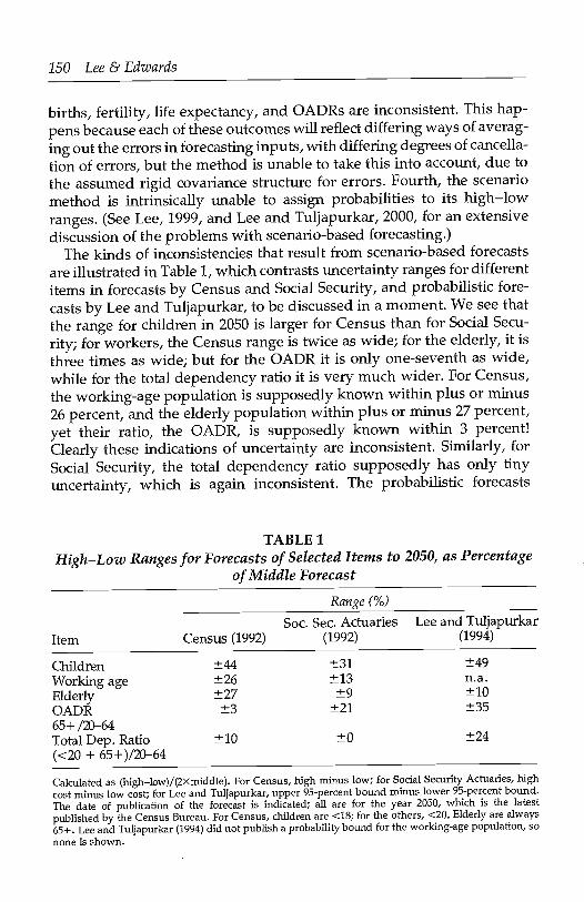
The kinds of inconsistencies that result from scenario-based forecastsare illustrated in Table 1, which contrasts uncertainty ranges for differentitems in forecasts by Census and Social Security, and probabilistic fore-casts by Lee and Tuljapurkar, to be discussed in a moment. We see thatthe range for children in 2050 is larger for Census than for Social Secu-rity; for workers, the Census range is twice as wide; for the elderly, it isthree times as wide; but for the OADR it is only one-seventh as wide,while for the total dependency ratio it is very much wider. For Census,the working-age population is supposedly known within plus or minus26 percent, and the elderly population within plus or minus 27 percent,yet their ratio, the OADR, is supposedly known within 3 percent!Clearly these indications of uncertainty are inconsistent. Similarly, forSocial Security, the total dependency ratio supposedly has only tinyuncertainty, which is again inconsistent. The probabilistic forecasts

TABLE 1High-Low Ranges for Forecasts of Selected Items to 2050, as Percentage

of Middle Forecast

(<20 + 65+)/20-64

Calculated as (highlow)/(2Xmiddle). For Census, high minus low; for Social Security Actuaries, highcost minus low cost; for Lee and Tuljapurkar, upper 95-percent bound minus lower 95-percent bound.The date of publication of the forecast is indicated; all are for the year 2050, which is the latestpublished by the Census Bureau. For Census, children are <18; for the others, <20. Elderly are always65+. Lee and Tuljapurkar (1994) did not publish a probability bound for the working-age population, sonone is shown.

R2nge (%)

Soc. Sec. Actuaries Lee and TuljapurkarItem Census (1992) (1992) (1994)

Children ±44 ±31 ±49Working age ±26 ± 13 n.a.Elderly ±27 ±9 ±10OADR ±3 ±21 ±3565+ /20-64Total Dep. Ratio ±10 ±0 ±24

The Fiscal Effects of Population Aging in the U.s. 151

shown in the last column have fully consistent indications of uncer-tainty, taking into account all covariances.

Although the traditional and widely used scenario method for assess-ing uncertainty of forecasts is seriously flawed, there are two othergeneral approaches that are more useful. The first is analysis of theperformance of past forecasts, and from that analysis, development ofprobability distributions for current forecasts on the assumption that themethods used and other circumstances are sufficiently similar in the pastand future to make this useful. This approach is illustrated by the proba-bility distributions provided for Congressional Budget Office (CBO) fore-casts of the federal surplus (CBO, 2001). The CBO had only a shorthistorical record of forecast performance to analyze, so its probabilitydistributions were provided for only five years ahead, a serious limita-tion. Another difficulty is that a separate historical analysis of forecasterrors must be conducted for each variable of interest. For an applicationof this approach in demography, see National Research Council (2000,chapter 7). For an application to the Social Security Actuaries' forecastingrecord, see Lee and Tuljapurkar (2000). The second approach is to de-velop stochastic forecasts that incorporate errors in the forecast of eachinput, and reflect their propagation through the forecast process.

Here we will follow a variant of this second approach, in which time-series methods are used to fit stochastic models for each input variable,and the propagation of errors is tracked through stochastic simulation.With this approach, a probability distribution can be calculated for anyoutcome of interest, including joint probability distributions for multipleoutcomes. In most cases, we constrain the central trajectory for eachinput (that is, the long-run mean) to match an assumption by the SocialSecurity Actuaries, the Centers for Medicare and Medicaid Services (pre-viously the Health Care Financing Administration), or the CongressionalBudget Office, but this is not the case for mortality. In all cases, thevariances and covariances are estimated from the historical data series.

4. STOCHASTIC POPULATION FORECASTSThe population forecasts we report below are distinctive in two respects.First, they reflect the choices for central trends in fertility, mortality, andimmigration that we have just discussed, which differ from those in theprojections by Social Security (in having lower mortality) and the CensusBureau (in having lower fertility). Second, they are probabilistic fore-casts based on a new method (Lee and Tuljapurkar, 1994).

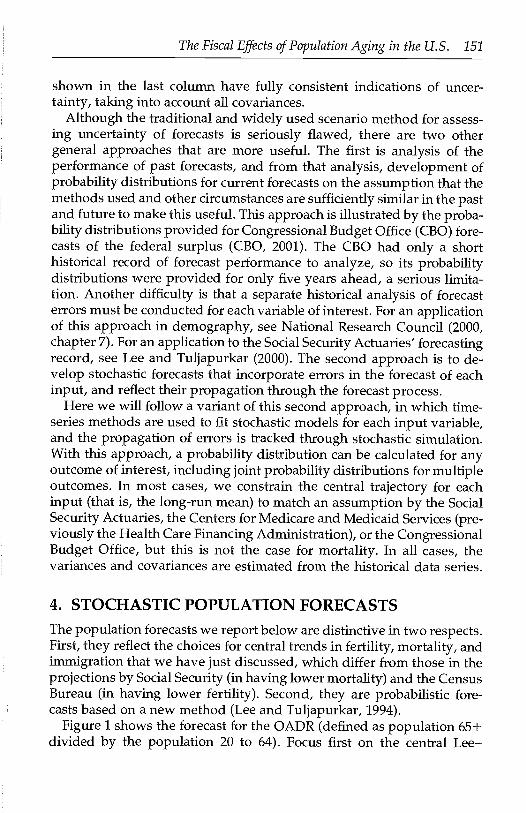
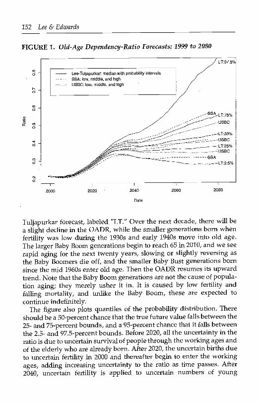
Figure 1 shows the forecast for the OADR (defined as population 65 +divided by the population 20 to 64). Focus first on the central Lee-

152 Lee & Edwards

FIGURE 1. Old-Age Dependency-Ratio Forecasts: 1999 to 2080

Lee-Tuijapurkar: median with probability intervalsSSA: low, middle, and highUSBC: low, middle, and high

LT:50%

USBC

LT:25%USBC

SSA

- -SSA LT:75%

.--USBC

LT:25%

LT:97.5%

2000 2020 2040 2060 2080

Date

Tuijapurkar forecast, labeled "LT." Over the next decade, there wifi bea slight decline in the OADR, while the smaller generations born whenfertility was low during the 1930s and early 1940s move into old age.The larger Baby Boom generations begin to reach 65 in 2010, and we seerapid aging for the next twenty years, slowing or slightly reversing asthe Baby Boomers die off, and the smaller Baby Bust generations bornsince the mid 1960s enter old age. Then the OADR resumes its upwardtrend. Note that the Baby Boom generations are not the cause of popula-tion aging; they merely usher it in. It is caused by low fertility andfalling mortality, and unlike the Baby Boom, these are expected tocontinue indefinitely.

The figure also plots quantiles of the probability distribution. Thereshould be a 50-percent chance that the true future value falls between the25- and 75-percent bounds, and a 95-percent chance that it falls betweenthe 2.5- and 97.5-percent bounds. Before 2020, all the uncertainty in theratio is due to uncertain survival of people through the working ages andof the elderly who are already born. After 2020, the uncertain births dueto uncertain fertility in 2000 and thereafter begin to enter the workingages, adding increasing uncertainty to the ratio as time passes. After2040, uncertain fertility is applied to uncertain numbers of young

0

(00

0

0

0

co0


women, compounding the uncertainty in the ratio. Finally, after 2065 thehighly uncertain size of birth cohorts begins to affect the projected num-bers of elderly in the numerator as well as workers in the denominator.Note also that there is nearly twice as much uncertainty in the upwarddirection as in the downward direction.4 By 2075, there is a 2.5-percentchance that the increase in the OADR wifi be twice as large as the centralforecast, and a 2.5-percent chance that it wifi be only one-fourth as largeas forecast. In any case, however, it is virtually certain that substantialpopulation aging wifi occur over the next forty years.

For comparison, Figure 1 also plots the central projections by SocialSecurity (SSA) and Census (USBC), along with their non-probabilistichigh and low projection variants. We note that there are not majordifferences in the central forecasts, but that after 2040, the Census andSocial Security projection ranges have much less than 95-percent proba-bility coverage. The upward range for both Census and Social Security isclose to the LeeTuljapurkar 75-percent bound, meaning that the truevalue would be expected to exceed the high bound for these projectionsabout 25 percent of the time, if the LeeTuijapurkar probability distribu-tion is correct.

5. HOW POPULATION AGING AFFECTSGOVERNMENT BUDGETS

It is straightforward and natural to use population projections to projectthe future costs of benefits, on the assumption that program structureswill remain as they are now. Such projections are useful for tracing outthe implications of current policies, and thereby informing decisionsabout changing those policies. These exercises should be viewed only asconditional forecasts, however. Studies of the effect of population agingin the past on government budgets show much smaller effects, becausein practice programs are adjusted. For example, Gruber and Wise (2001)examined data for OECD countries over time, and found that a 10-percent increase in the proportion of elderly in the population led to a 5-percent increase in expenditures on the elderly, so that expenditures perindividual old person declined while the aggregate expenditure on theelderly increased (that is, they found an expenditure elasticity of 0.5,measured relative to GDP). They also found that spending in other areasof the budget was reduced, so that total government expenditures as ashare of GDP did not change with population aging.

This is typical of the probability distributions for population forecasts. Population growthis multiplicative, so uncertainty is lognormally distributed.

154 Lee & Edwards

FIGURE 2. Benefits bj Program and Age

0000CU

00U)

000

000U)

0 -Other benefits such as public assistance and congestibles.

Medicare

Social Security

0 20 40

Age

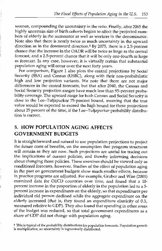
Evidently population change does not dictate outcomes, but ratheralters the trade-offs and constraints faced by policymakers. In the rest ofthis section, we will consider how this works. We begin by presenting thecurrent cost of benefits received by age in the U.S., 13(x), and tax pay-ments by age, T(x). Figure 2 plots 13(x), broken down by broad category ofexpenditure, but originally based on 25 individual or household benefitprograms (school lunches, TANF, energy assistance, SSI) plus additionalnon-individual programs (roads, police, etc.) (see the Appendix for expla-nation of how these were estimated). The data refer to average amountsper surviving individual at each age, so keep in mind that there arerelatively few survivors to very old ages. They include all governmentexpenditures at the federal, state, and local levels, except for expendi-tures on public goods (mostly defense spending). Expenditures which donot accrue to individuals or households are assigned on a per capitabasis.The concentration of expenditures on children and on the elderly is appar-ent. The average elderly person receives over $20,000, which is about fourtimes as much as the average child. Note that Medicaid expenditures forelderly people are primarily for nursing-home care.

Figure 3 plots 7(x), again per surviving individual at each age, andbroken down by kind of tax (see the Appendix for details of construc-

60 80

FIGURE 3. Taxes by Program and Age

c00 -

000


Other taxes including federal corporate tax and charges/fees.

0

I I I

20 40 60 80

Age

tion). Note that for some kinds of taxes, the elderly pay about the sameamount as prime-age adultsnotably corporate tax (inferred from divi-dend income), property tax, and sales tax. However, because theydon't have much labor income, they pay far less payroll tax and incometax, and in total pay much lower taxes than prime-age adults.

To see how population aging will affect the costliness of our currentagebenefit structure, we can calculate how the changing populationage distribution would alter the ratio of total taxes to total benefit expen-ditures. We will call this ratio the fiscal support ratio. We could imagine anindividual or a planner weighing the utility of receiving the benefit sched-ule 13(x) over the life cycle, vs. receiving the after-tax income that wouldbe released by reducing or eliminating the programs that 13(x) comprises.While individual utility from the stream of benefits is distributed overfuture years of the life cycle, the cost in taxes is determined by the cross-sectional balanced-budget constraint in each year, which is in turn deter-mined by the population age distribution. This interplay between theindividual life cycle and the cross-sectional population age distributiongenerates the fiscal effects of population aging. In an important sense,the population age distribution determines the price of the vector of life-cycle benefits, 13(x). This price is the ratio of aggregate taxes to benefits,

156 Lee & Edwards

FIGURE 4. Projected Fiscal Support Ratio b!,' Level of Government,2000 to 2100

1.1

00

0.8

0.7

State and Local

Federal

2100I I I I P

2000 2010 2020 2030 2040 2050 2060 2070 2080 2090Year

Note: The fiscal support ratio is calculated as the ratio of tax revenues to government expenditures,based on the age-specific tax and expenditure profiles for 2000, applied to the projected age distributionfor each period.

evaluated for the changing population age distributions in the future,using the current age profiles of taxes and benefits, 13(x) and 7(x). Asimilar calculation could be made using the projected profiles of taxesand benefits for some later year, and that would give somewhat differentresults.

Figure 4 plots the changing ratio of taxes to benefits over the next cen-tury, based on the central population forecast. It can be seen that there ishardly any effect at the state and local level; the ratio is quite constantover the century. At the federal level, however, population aging leadsto a far bigger increase in benefit costs than in tax revenues. The samelevel of taxes represented by 7(x) would buy a level of benefits, 13(x), only64 percent as high in 2075 as in 2000. Put differently, we might say thatpopulation aging wifi raise the price of this benefit bundle 13(x) by 56


percent (0.64 = 1/1.56) over this century, in terms of after-tax income.5As population aging alters this price, we might expect voters and policymakers to choose a lower level of the benefit age profile (x), and corre-spondingly more after-tax income for taxpayers.6 The net effect on aggre-gate benefit expenditures would be ambiguous. Although there will be agreater number of elderly people, each of them would receive lowerbenefits, and consequently the net effect of population aging on bothaggregate benefit expenditures and on aggregate taxes and tax rateswould be ambiguous. This interpretation, although ignoring the costs oftransitions between program regimes, is broadly consistent with Gruberand Wise's (2001) results described above.

Note also that Figure 4 is based on the current program structure, andso it does not reflect the large expenditure increases per beneficiary thatare projected for Medicare and Medicaid over the course of the twenty-first century, due to projected increases in the quality and quantity ofservices consumed (Lee and Miller, 2001b).

Figure 4 showed a single forecast of the support ratio, as if we actuallyknew what the future would bring. Figure 5 presents probabilistic fore-casts of the support ratio, showing the median value (which was plottedin Figure 4) along with 95-percent probability intervals. In early years,uncertainty results largely from uncertainty about fertility; the effects ofuncertain mortality emerge only over the longer run. Variations in fertil-ity have a strong effect on state and local finance once they affect thenumber of children of school age, that is, at age 5 or older. Thus theprobability band for the state and local support ratio is very narrow forthe first five years of the forecast, and opens up rapidly thereafter. Thenumber of children has relatively little effect on the federal budget untilthey grow old enough to enter the work force and begin paying taxes,beginning around age 20. Even then, the steep slope of 7(x) implies thatuncertain fertility does not have a large effect on taxes for a number ofyears after that. Thus, the probability interval for the federal supportratio is very narrow for the first thirty years or so, and then widens asuncertainty about the size of the labor force grows. Uncertain mortality

Strictly speaking, this interpretation makes sense only when all difference in populationage distributions is due to change in fertility, not mortality, and the system is unchangingover time. When mortality is declining, then the expected value of the benefit package overthe life cycle wifi rise, since the expected duration of receiving benefits in old age increases.When the program system is changing over time, then the link between individual benefitsover the life cycle and the current benefit package is not tight.

In reality, the shape of /3(x) could also be changed, for example by favoring programs forchildren at the expense of programs for the elderly. Population aging also alters the cost ofproviding benefits to a child relative to the cost of providing benefits to an elderly person.

158 Lee & Edwards

FIGURE 5. Projected Fiscal Support Ratio by Level of Government,2000 to 2100 (Median and 95% Probability Interval)

Federal

State and local

Note: The Fiscal Support Ratio is calculated as the ratio of tax revenues togovernment expenditures, based on the age specitic tax and expenditure profilesfor 2000, applied to the projected age distribution for each period. Stochasticpopulation projections were bused on the methods in Lee and Tuljapurkar, 1994.

I I I I I

2000 2020 2040 2060 2080 2100

Year

Note: The fiscal support ratio is calculated as the ratio of tax revenues to government expenditures,based on the age-specific tax and expenditure profiles for 2000, applied to the projected age distributionfor each period. Stochastic population projections were based on the methods in Lee and Tuijapurkar(1994).

contributes a small amount of uncertainty to the support ratio, but notmuch.

It is clear that demographic change is almost certain to cause seriouspressures on the federal budget as the Baby Boom generations enter oldage. Through 2040 or so, budgetary pressures can be projected withgreat confidence. After this it is not so clear whether pressures wificontinue to mount, or somewhat abate.

At the state and local level, the median support ratio shows no trend,but there is a great deal of uncertainty. It is not clear that there would beany advantage to planning for a growing school-age population, whenthat population is just as likely to decline, relative to taxpaying workers.

Co.4-a

1

ci)

0 C"4-a

Co1

ci)><CjI- 000

cc0 0

.4-a

00

C,)

0U) 0

LL


In the long run, there is a negative correlation between errors in fore-casting the state and local fiscal support ratio and the federal one. Highfertility is costly for the state and local entities providing public educa-tion, but it allows lower taxes at the federal level, since it generates moreworkers to support the elderly. Thus, there is less uncertainty in thetotal fiscal support ratio than one would expect from looking at its con-stituent parts.

6. CONSTRUCTING STOCHASTIC BUDGETARYFORECASTSWe can build on these stochastic population forecasts to developstochastic projections of government expenditures, assuming that thebasic structure of programs is unchanged. To do so we need first todevelop the linkage of population forecasts to costs of benefits, andsecond to incorporate some sources of economic uncertainty.7 Popula-tion is linked to benefit costs by the age schedule of costs of benefitscurrently received by a person in age group x. This average benefitprofile is the 13(x) presented earlier in Figure 2. This schedule cannot beexpected to remain fixed in the future, however, even under the assump-tion that program structure remains fixed. Benefits for most programscan be expected to rise as productivity increases. We will follow CBO inassuming that most benefits rise in real cost at the same rate as productiv-ity growth, which raises per capita incomes and labor costs. Some pro-grams, notably social security, Medicare, and Medicaid, require specialtreatment, however, as we now discuss.

For social security, we take into account the legislated change in thenormal retirement age from 65 to 67 in the coming decades. Our projec-tions of benefits are based on the actual rules governing benefits inrelation to prior earnings (see Lee and Tuljapurkar, 1998a and 1998b, fordetails), and indirectly take into account such particulars as the notchgeneration, the selective effect of mortality at older ages, and the effectsof loss of spouse on benefit levels.

Benefit costs for Medicare have typically been rising much more rapidlythan productivity growth, and are expected to do so for the foreseeablefuture. We constrain our median projection for health care costs per en-rollee at each age to follow the CBO (2000) assumptions (which are verysimilar to the 2001 HCFA/CMMS projection assumptions in Board of Trust-ees of the Federal Hospital Insurance Trust Fund, 2001) in which the rate

For a number of years, CEO published stochastic long-term forecasts based on these Lee-Tuljapurkar stochastic population forecasts, with deterministic economic variables.

160 Lee & Edwards

of increase per enrollee declines to an eventual level 1 percent per yearmore rapid than the growth rate of productivity. We differ, however, intaking into account the distribution of the population at each age by timeuntil death. The Medicare costs of individuals have been shown to beclosely associated with their proximity to death (Lubitz and Prihoba, 1984;Lubitz, Beebe, and Baker, 1995; Miller, 2001). In a projection, we know foreach year what proportion of people at a given age will die within oneyear, one to two years, ten years, and so on, and can allocate health costsaccordingly. Time until death thus serves as a kind of index of healthstatus. We apply the rate of increase of per enrollee cost to each categoryof time until death separately (see Lee and Miller, 2001b, for details).

For Medicaid, we note that the proportion of the elderly population inlong-term care facilities at each age has been declining for some time,presumably due to the improving health of the elderly population. Weproject this decline to continue, which partially offsets the increasingcosts of care for those in institutions.

7. DETERMINISTIC FORECASTS OF THE FISCALEFFECTS OF AGING

We will begin by considering some deterministic projections, then turnto stochastic ones.

Figure 6 plots projected government expenditures as shares of GDP forthe federal government, and for state and local governments grouped to-gether, as well as their sum. Excluded from these totals are interest pay-ments on the federal debt, and benefits paid for pre-funded programssuch as most state and local pensions and some insurance funds. Totalexpenditures are initially 25 percent of GDP, but are projected to riseabove 40 percent of CDP by 2075 and to continue climbing thereafter. Forthe federal budget and overall, there is an acceleration in the rate ofincrease between 2010 and 2030 when the Baby Boom is reaching old age,but clearly that is only a part of the story, since the trend continues rapidlyupward after 2040. At the state and local level, expenditures rise onlymildly relative to GDP. Almost all the increase in the total is due toincreases at the federal level, which is not surprising given the importanceof federal transfers to the elderly. Federal expenses increase from 16 per-cent of GDP in 2000 to 30 percent iii 2075, almost a doubling, and by 2100they are approaching 40 percent.

It is also interesting to separate these expenditures by age group of therecipients. We define three categories: spending on the elderly, spend-ing on children, and programs that are age-neutral. We have assigned

0.2

0.1

02000 2010


FIGURE 6. Government Expenditures as Shares of GDP

0.5

0.4

State and Local

2050 2060Year

2070 2080 2090 2100

each program to one of these three categories, based either on the natureof the program or on some criterion such as the average dollar-weightedage of the recipient.

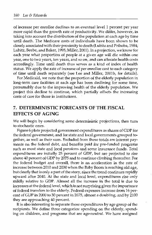
Figure 7 shows the result for all levels of government combined. Ex-penditures for children are flat over the next 100 years, relative to GDP.Age-neutral expenditures show some growth, but only to the extent thatthey include the non-institutional component of Medicaid, which growsfaster than GDP due to excess growth in per capita health care costs.Almost all the projected increase in government spending over the next75 years and beyond is due to increased expenditures on programs forthe elderly. These rise from about 8 percent of GDP in 1999 to 21 percentof GDP in 2075, and they more than triple their share by 2100.

It is also illuminating to look at the growth in expenditures by kind ofprogram, rather than by age of recipient. Figure 8 shows the growth inprojected expenditures for retirement programs (OASDI, federal employ-ees, and railroad workers), health programs for the elderly (MedicareParts A and B and institutional Medicaid), other expenditures for the

20402020 2030

162 Lee & Edwards

FIGURE 7. Government Expenditures per GDP b Age Group

0.3

0.25

0.1

0.05

Elderly

200 2010 2020 2030 2040 2050 2060 2070 2080 2090 2100Year

elderly, and all other federal expenditures. It is striking that the growthin expenditures for retirement programs, including social security, issuch a small part of the projected growth in federal spending, contraryto the attention allocated to retirement programs in public discussions.Retirement accounts for only one-eighth of the total growth, with mostof the rest due to growth in health care for the elderly. This very lowshare is in part due to the assumption of a 2.3-percent mean rate ofproductivity growth, which is 1.0 percent higher than the Social SecurityActuaries' assumption, and which in itself would improve the summaryactuarial balance measure from 1.89 percent of the present value ofpayroll to only 0.89 percent, making more than half of the projectedimbalance disappear. Without this assumption, retirement programswould account for about a quarter of the projected expenditure increase.The projected increases in health care for the elderly are roughly halfdue to population aging (reflecting low fertility rather than mortalitydecline) and half to increases in costs per enrollee in excess of productiv-ity growth (Lee and Miller, 2001b). The new assumptions by CBO and

AgeNeutral

Children

0.2000

0.15


FIGURE 8. Federal Expenditures per GDP by Type of Spending

2000 2010 2020 2030 2040 2050 2060 2070 2080 2090 2100Year

HCFA/CMIvIS on this excess rate of cost growth have a powerful influ-ence on these projections.

8. STOCHASTIC BUDGETARY PROJECTIONSSo far we have not discussed how economic uncertainty is incorporatedin our projections. We treat productivity growth and (where relevant)real interest rates and stock market returns as stochastic, following amodeling strategy similar to that used for fertility in the demographicprojections (see the Appendix for details). That is, we model these asstochastic time series, and fit the models on historical data. The modelswe fit are constrained to have mean values that are consistent either withcomparable official projections or the historical record, depending on thepurpose of the forecast. Matching social security, our real interest rateaverages 3 percent per year; we set labor productivity growth at 2.3percent per year, roughly its postwar average; and real stock market

0.4

0.3

00

+ NonElderly0,ci)

ci)

+Other-ci)

E

0+ Health Care

0.1

Retirement

164 Lee & Edwards

returns are 7 percent per year, reflecting historical trends in the S&P 500.Thus for the most part, our fitted models are providing the structure oferrors for our forecasts of economic inputs, but not their mean or medianvalues, which are rather imposed. For the productivity growth rate, thestandard error of the one-step forecast is 1.78 percent, so a 95-percentprobability interval has a width of 7 percent, wide indeed. For theinterest-rate model, the one-step forecast has a standard error of 2.04percent, so the width of a 95-percent interval is over 8 percent. Theseintervals are very much wider than the highlow assumption ranges ofSocial Security, which have a width of 1 percent for productivity growthand 1.5 percent for real interest rates. However, it must be borne in mindthat the stochastic interval refers to realized values in a single year,whereas the Actuaries' assumptions can best be thought of as referringto a long-run average.

The actual stochastic forecast is then carried out through stochasticsimulation. A single stochastic trajectory is calculated by drawing ran-dom numbers to determine the forecast errors for the first year, whichare then inserted in the appropriate equation for each input, along withthe previous years' values, leading to a one-step forecast. Then theforecasts of population and benefit costs are derived mechanically fromthese forecasts of inputs. Then a second round of random numbers isdrawn to generate the second year of the forecast, and so on. In thisway one stochastic trajectory is forecast. We generate many such trajec-tories, generally at least a thousand, and then use the frequency distri-bution for outcomes of interest to estimate the probability distribution ofthe forecast. Outcomes include total expenditures on benefits, expendi-tures for a particular program, the date of Trust Fund exhaustion forsocial security, or the Trust Fund ratio, and so on. If desired, we canalso project tax revenues in a similar way, and we can constrain tax ratesto be adjusted so as to maintain some target such as a pre-specifieddebt-to-GDP ratio.

9. STOCHASTIC PROJECTIONS FORSOCIAL SECURITY

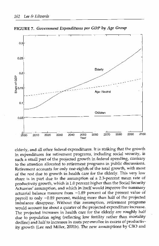
We now turn to stochastic long-term projections of the finances of thesocial security system, drawing on Lee and Tuljapurkar (1998a, 1998b).We have already described the methods we have used, so we can movedirectly to results. Perhaps the most basic statistic is the cost rate, that is,the costs of benefits in a given year as a percentage of payroll in thatyear. In a pure pay-as-you-go system, with no accumulated trust fund,

35

20

15


FIGURE 9. Cost Rate (Outgo as a Percentage of Taxable Payroll)

this would be the payroll tax rate for each year. Figure 9 plots variousprobability quantiles and the mean of the cost rate for each year through2075, with a projection base year of 2000. These runs are based on theproductivity growth-rate assumption of Social Security, so aside fromour forecast of more rapid mortality improvement, our central forecastsshould match closely those of the Social Security Actuaries for the samebase year (Board of Trustees, 2000). The results reported here weregenerated by a stochastic simulation program written by Michael Ander-son and Shripad Tuljapurkar,8 which can be accessed free via the In-ternet at http: / /simsoc.demog.berkeley.edu.

Users can modify many aspects of the policy environment, includingplans for investing a portion of the Trust Fund in equities, raising theage at retirement, and raising the payroll tax rate.

8 The results presented in Figures 9-12 are based on the output of this program, which iscurrently in beta testing and not guaranteed to be bug-free.

2000 2010 2020 2030 2040

Year2050 20&3 2070

166 Lee & Edwards

We see that by 2075, the median cost rate is 21.2 percent. There is a 2.5-percent probability that the cost rate wifi be only 14.6 percent, but also a2.5-percent probability that it wifibe at least as high as 36.5 percent. Thesefigures can be compared with the Social Security projections (Board ofTrustees, 2000), which give 19.5 percent for the intermediate trajectoryand 13.9 to 28.3 percent for the range. Our central forecast is about 2percent higher, due to the more rapid decline in mortality that we project.Our lower 2.5-percent bound is similar to the SSA low cost scenario, butour high 2.5-percent bound is almost 7 percent higherconsistent withFigure 1, which showed much larger uncertainty in the upward directionfor the OADR than indicated by either Social Security or Census. Byconstruction (see the Appendix) the long-run means of our forecasts forfertility, for the productivity growth rate, and for the real interest rate areidentical to those assumed by the Social Security Actuaries, while ourprojected life expectancy for 2075 is about three years higher.

We have compared our outcomes with those of the Actuaries, but it isimportant to note that ours are probabilistic whereas theirs are determin-istic ranges and have no probabilistic meaning. It appears that the Actu-aries' low cost scenario matches our lower 2.5-percent bound for the costrate, while their high cost scenario corresponds roughly to our upper 86-percent bound. That is, the chances that the cost rate wifi exceed theActuaries' high cost boundary are more than five times greater than thechances of its failing to reach the low cost boundary.

There is relatively little uncertainty in the income rate, that is, tax in-come as a proportion of payroll, since the only uncertainty comes fromrevenues from taxes on benefits. However, the highly uncertain cost rateleads to large uncertainty in the various measures of net outcome. Forexample, our forecasts find a median date of fund exhaustion undercurrent policy of 2038, very close to the intermediate projection of theActuaries, 2037. We find a 2.5-percent chance of exhaustion by 2024,versus 2027 for the high cost projection of the Actuaries. We also findroughly a 4-percent probability of exhaustion after 2075, compared to noexhaustion by 2075 for the Actuaries' low cost projection, which also hasa healthy Trust Fund ratio at that point.

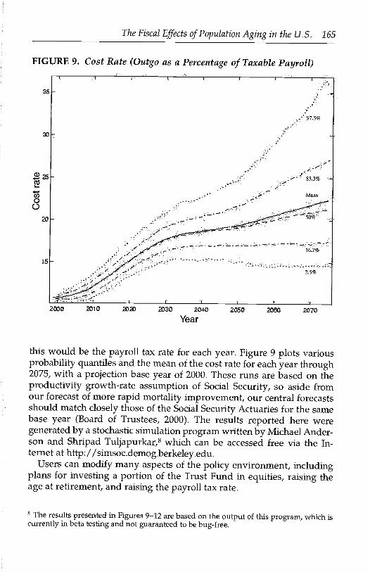
The Actuaries finds that an immediate rise in the payroll tax of 1.89percentage points should restore actuarial balance over the 75-year hori-zon. We have also simulated the outcome assuming taxes are raised inthis manner, from the current rate of 12.4 percent to 13.29 percent.Figure 10 depicts a histogram of the 1,000 probabilistic dates of exhaus-tion generated by our model under such a policy. Our method makesexplicit what may be fairly intuitive: An immediate rise in payroll taxesdesigned to restore actuarial balance wifi only prevent Trust Fund bank-

FIGURE 10. Histogram of 1,000 Dates of Exhaustion with ImmediatePayroll Tax Increase of 1.89%


2030 2040 2050 2060 2070 2080 2090 2100+

Year

ruptcy roughly 50 percent of the time. More strikingly, the lognormaldispersion of exhaustion dates in Figure 10 implies that the mode of thedistribution actually occurs much earlier than 2075. Even a painfullylarge hike in the payroll tax today does not move the most frequentlyrealized future date of bankruptcy past about 2055.

Figure 11 displays a histogram showing 1,000 realizations of the 75-year actuarial balance dating from 2000, under the prescribed 1.89-percentage-point rise in the payroll tax. The long left tail indicates thatthe chances of undershooting actuarial balance, denoted by 0 on thehorizontal axis of the graph, are more widely dispersed than the chancesof overshooting. That is, although the risks are roughly balanced underan immediate payroll tax hike, the downside risks are more costly.

Our stochastic framework lends itself particularly well to analyses involv-ing social security's finances and risk. During the Clinton administration,

00-(Y)

0C\J 2.5% by 2036

0 16.7% by 20480- 50.0% by 207083.3% after 2099+

0 97.5% after 2099+U)1

001

0U)

0

168 Lee & Edwards

FIGURE 11. Histogram of Actuarial Balances with Horizon to 2074

z.

- -iActuarial balance

policymakers considered plans to invest part or all of the Trust Fund inequities, and currently the Bush administration is said to be weighingthe option to replace part of the system with private accounts. An assess-ment of the riskiness of such plans is important in light of the uncer-tainty of stock market returns. Figure 12 presents a histogram of TrustFund exhaustion dates under a particular investment plan: immediatelyplacing 20 percent of the entire Fund balance in the S&P 500 in 2000, andincreasing that share to 50 percent by 2010. The most striking characteris-tic of Figure 12 is that the distribution peaks soon around 2030-2035 andthen tapers off very rapidly, even though the median date of Fundexhaustion is 2044. This dynamic is due to the risky nature of stockreturns, which may potentially help social security's finances consider-ably, but at the same time wifi not change the expected date of bank-ruptcy very much. We have also simulated the effects of investing 75

percent of the Trust Fund in equities immediately. This leads to a meanfund balance equal to three times GDP in 2074. However, the median

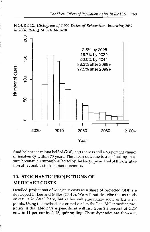
FIGURE 12. Histogram of 1,000 Dates of Exhaustion: Investing 20%in 2000, Rising to 50% by 2010

00-C\i


83.3% after 2099+97.5% after 2099+

00

0LU

0

2020 2040 2060 2080 21 00+

Year

fund balance is minus half of GDP, and there is still a 63-percent chanceof insolvency within 75 years. The mean outcome is a misleading mea-sure because it is strongly affected by the long upward tail of the distribu-tion of favorable stock market outcomes.

10. STOCHASTIC PROJECTIONS OFMEDICARE COSTS

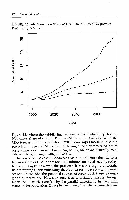
Detailed projections of Medicare costs as a share of projected GDP aredeveloped in Lee and Miller (2001b). We wifi not describe the methodsor results in detail here, but rather wifi summarize some of the mainpoints. Using the methods described earlier, the LeeMiller median pro-jection is that Medicare expenditures wifi rise from 2.2 percent of GDPnow to 11 percent by 2075, quintupling. These dynamics are shown in

2.5% by 2025

0-IA)-

1

16.7% by 203250.0% by 2044

170 Lee & Edwards

FIGURE 13. Medicare as a Share of GDP: Median with 95-percentProbability Interval

0C"

2000 2020 2040 2060

Year

Figure 13, where the middle line represents the median trajectory ofMedicare's share of output. The LeeMiller forecast stays close to theCBO forecast until it terminates in 2040. More rapid mortality declinesprojected by Lee and Miller have offsetting effects on projected healthcosts, since, as discussed above, lengthening life spans generally coin-cide with lengthening healthy life spans.

The projected increase in Medicare costs is huge, more than twice asbig, as a share of GDP, as are total expenditures on social security today.Not surprisingly, however, the projected increase is highly uncertain.Before turning to the probability distribution for the forecast, however,we should consider the potential sources of error. First, there is demo-graphic uncertainty. However, note that uncertainty arising throughmortality is largely canceled by the parallel uncertainty in the healthstatus of the population: If people live longer, it wifi be because they are


in better health, or so the time-until-death approach assumes. Second,note that uncertainty about the rate of productivity increase is also fil-tered out, once we express the costs relative to GDP. If productivitygrowth is 1 percent per year more rapid than expected, then by assump-tion health costs will also grow 1 percent per year more rapidly thanexpected, as will GDP. The ratio of total costs to GDP is unaffected.Therefore the most important sources of uncertainty in the ratio of coststo GDP will be fertility and the size of the gap between the rates ofincrease in per-enrollee costs and productivity growth. We have fitted atime-series model to this gap over the past 50 years and then used it toassess the variance structure of the gap.9

With this background, we found that the 95-percent probability inter-val for the cost-to-GDP ratio in 2075 is 5 to 26 percent, as shown in Figure13. That is, there is a 97.5-percent chance that the ratio will at leastdouble, and a 2.5-percent chance that it wifi increase at least twelvefold.The uncertainty in the upward direction is more than twice as great as inthe downward direction, similar to results we have seen before. Thisrange of uncertainty reflects the U.S. experience with cost containmentin the 1990s as well as earlier periods of more rapid growth. It is indeeddifficult to plan for the future when there is so much uncertainty.

Comparing our 95-percent intervals with the CBO projections, wefind that while in later years of their forecasts their highlow range issimilar to our 95-percent range, for earlier years their range greatlyunderstates the uncertainty. This is a common problem with the sce-nario approach for assessing uncertainty in projections.

11. DISCUSSIONPopulation aging is virtually certain to occur in the coming decades, andit wifi have a serious impact on the costliness of many governmentprograms. We have assessed the fiscal pressures of population aging byexamining its impact on many age-assignable government programs, aswell as on tax receipts. However, recent economic change has under-lined the dangers of ignoring the role of chance in formulating our plans.Many projections simply assume that the short-run or long-run futurewifi unfold according to the pattern of the past few years, which is arisky practice. Good forecasts ought to provide some measure of thisrisk. Yet the scenario method, which is most widely used to incorporate

We have followed the suggestion of the Technical Advisory Panel for HCFA/CMMS inusing a more general measure of health costs to calculate this gap, rather than specificallyMedicare costs, and therefore we are able to go back in time before Medicare was launchedin 1965.

172 Lee & Edwards

uncertainty in government forecasts, is seriously flawed. We, togetherwith collaborators, have developed new and explicitly probabilistic meth-ods for forecasting population and government expenditures, based onanalysis of historical variability combined in many cases with expertjudgement about central trends. Thus our analysis has had two goals: toexamine the fiscal effects of population aging, and to do this in a probabi-listic setting using stochastic simulation.

Beginning with the demography, we find that the OADR is virtuallycertain to increase by more than 50 percent in the 2030s. While it ispossible that it wifi decline a bit thereafter as the Baby Boom generationsdie, more likely it will continue to increase after 2050, possibly by a greatdeal. The chance of very high ratios is substantially greater than indi-cated by Census or Social Security projections. Population aging raisesthe cost of the current structure of government programs (includingthose for children) relative to tax revenues, and makes a given packageof life-cycle benefits more costly relative to the life-cycle tax paymentsnecessary to fund it. We find that population aging is virtually certain toincrease the costliness of current federal programs by 35 percent (±2percent) by the 2030s, and with less certainty by 60 percent (± 15 percent)in the second half of the century. Although population aging will notaffect the costliness of average state and local programs in the mean ormedian forecast, there is considerable uncertainty about this (±20 per-cent or so) after 2020. We expect that governments wifi respond to theseaging-induced cost changes by altering program structures, as they havein the past.

Although it is unlikely that the current program structure wifi remainunchanged, it is nonetheless useful to project the consequences of main-taining it. Under this assumption (while the retirement age rises as cur-rently legislated and health care costs per enrollee rise as projected),federal expenditures are projected to rise dramatically relative to GDP,from 16 percent of GDP in 2000 to 30 percent in 2075, almost a doubling,and by 2100 they are approaching 40 percent (these figures excludeinterest payments on the debt and payments into pre-funded pro-grams). State and local expenditures rise only modestly relative to GDP.Almost all of this increase is for programs going primarily to the elderly,which rise from 8 percent of GDP in 1999 to 21 percent of GDP in 2075and which more than triple their share by 2100. Programs for health carefor the elderly account for the greatest part of this increase, with pen-sions a distant second.

Looking specifically at the social security system, although we believethe Actuaries underproject future mortality improvements, we are im-


pressed by the quality of their projections. However, we find that theyunderestimate the risk of very costly outcomes. According to our proba-bilistic projections, the chances that the cost rate will exceed the Actu-ary's high cost boundary are more than five times greater than thechances of its failing to reach the low cost boundary. Raising the payrolltax rate by 1.89 percent, which according to the Trustees Report of 2000would have put the system into 75-year actuarial balance, has relativelylittle effect on the probabilities of early exhaustion, raising the 2.5-percent bound of exhaustion from 2024 to 2036, while raising the mediandate of exhaustion from 2036 to 2070; there would still be a 55-percentchance of insolvency within the 75-year horizon, with a median TrustFund balance after 75 years of 6 percent of GDP. Investing some or allof the Trust Fund in equities may help solve the long-run problem interms of average outcomes, but not in terms of more important mea-sures such as the median outcome or the probability of insolvency.

Looking specifically at Medicare, which now costs 2.2 percent of GDP,we found a median share in 2075 of 11 percent, five times as great. The95-percent probability interval for 2075 is 5 to 26 percent of GDP, so thatthere is a 97.5-percent chance that the ratio wifi at least double, and a2.5-percent chance that it wifi increase at least twelvefold. The uncer-tainty in the upward direction is more than twice as great as in thedownward direction, reflecting lognormality, as we have seen before.

Because probabilistic forecasts have only recently become available,research on their uses and implications has barely begun. The immedi-ate impulse is to treat these forecasts as if they simply provided animproved highlow range. In fact, they contain much more informationthan that, and they can support more powerful uses and analyses.

One key question is how uncertainty should affect our planning.Should the possibility of worse outcomes lead us to take additional pre-cautionary measures today, or should the possibility of better outcomeslead us to postpone action until we are sure action wifi be necessary?(See, for example, Auerbach and Hassett, 2001). Another importantquestion is how different kinds of policies perform in the context ofuncertainty. Do some reduce the uncertainty and others amplify it? Forexample, indexing retirement benefits to life expectancy at retirement(as has been done in Sweden) wifi reduce uncertainty for the pensionsystem arising from future mortality, by passing on the consequences ofthe uncertainty from the taxpayers to the beneficiaries. Medicare coststurn out to be only slightly affected by uncertainty in future mortality,because of offsetting effects of health improvement on numbers of en-rollees and costs per enrollee. Using the stochastic simulations as a kind

174 Lee & Edwards

of experimental laboratory, various policies can be assessed in terms ofcriteria such as intergenerational equity, rapidity of changes in taxes,rates of return, and so on.

APPENDIX: METHODS USED FOR STOCHASTICPROJECTIONS

A.1 Demographic ProjectionsA.li Mortality Let m(x,t) be a central death rate for age [x,x+5) andtime [t,t+1). Suppose we have a matrix of X age-specific death rates overT years. The LeeCarter method estimates the model:

In = a + b1k + 8x,t (A.1)

using a singular-value decomposition (SVD) or some other appropriatemethod. This yields estimates of a, b, and k. A second-stage procedureadjusts k to match exactly the life expectancy at birth implied by thefor each year t.

We now have a time series of k over T years (for most purposes, wehave used data from 1950 to 1999; for some purposes, we start in 1900).This time series is modeled using standard BoxJenkins methods. (Testsfor covariance with the residuals from the fertility model described be-low showed no association, so they were modeled independently). Inmost applications, it is well fitted by a random walk with drift. The fittedmodel for k can then be used to forecast k over the desired horizon,together with a probability distribution for each forecast year:

= k1 1.029 +, s.e.e. = 1.366. (A.2)(0.195)

From the forecasts of k, using equation (A. 1), probability distributions andmean or median values of 1n and the implied life expectancies can becalculated, along with probability distributions. These probability distri-butions wifi typically reflect the innovation error in k, along with theuncertainty of the estimate of the drift in the k process. They typically willnot include the 8xt terms, nor the uncertainty in the estimates of the a andb, which do not add much to the uncertainty after the first decade or two.On all of this, see Lee and Carter (1992) and Lee and Miller (2001a).

A.1.2 Fertility A similar approach is followed, but the fertility ratesthemselves, rather than their logs, are modeled. The model for age-specific fertility g is


g = c + df, + (A.3)

which is again estimated using a SVD. Time-series models applied to thehistory of fertility in the U.S. do not provide a plausible model or fore-cast for fertility, for various reasons, so the mean of the forecast is con-strained to equal a level specified ex ante, and in practice is taken to equalthe ultimate level of fertility assumed by the Social Security Actuaries,currently 1.95 children per woman. The fitted time-series model thenprovides crucial information about the variability and autocovariance offertility. See Lee (1993) for a discussion of all these issues, and explora-tion of some alternative modeling strategies. The fitted fertility time-series model is

= 0.96f - 0.0037 + + 0.52v, (A.4)

where the standard deviation of v is 0.11.

A.1.3 Immigration Immigration was projected deterministically follow-ing the assumption of the Social Security Actuaries, since it was thoughtbetter to treat it as a policy instrument than to attempt to forecast futurepolicy.

A.t4 Population Forecasts Initial conditions for the forecast comefrom the base-period population age distribution, taken from social secu-rity data. A single stochastic sample path is generated by drawing ran-dom numbers for the errors in the fertility and mortality equations, andthereby generating a trajectory of age-specific fertility and mortality ratesover the desired horizon, say 100 years. Sample paths containing a totalfertility rate below 0 or greater than 4 are discarded. In remaining paths,any negative age-specific birth rates are set to 0. These are combinedwith the deterministic immigration rates. Using well-known accountingidentities, the population forecast by age group is then calculated for thissingle sample path. The procedure is then repeated many times, some-times 1,000 times and sometimes 10,000 times. The frequency distribu-tions of outcomes of interest then provide estimates of the probabilitydistributions for these outcomes, and joint distributions can be providedin a similar way.

A.2 Economic ProjectionsA.2.1 Productivit, A demographically adjusted productivity growthseries was constructed. First, an average wage profile by age and sex wascalculated from the 1997 March Current Population Survey (CPS). Data

176 Lee & Edwards

on the agesex composition of the labor force were also taken from theCPS, from 1948 to the present. The effect of the changing agesex compo-sition of the labor force, based on these agesex weights for wages, wasthen calculated for each year since 1948 and used to adjust the officialmeasure of productivity growth in the private non-farm business sectorto remove the effect of the changing demographic structure of the laborforce. The adjustment made little difference in general.

Next, a constrained-mean time-series model was fitted to the ad-justed productivity growth series. As with fertility, the time-seriesmodel provides information about the variance, autocovariance, andcross-covariance of the series, but not about the long-run mean, whichis imposed. An autoregressive model of order one was found to fit thedata best:

g - = /3:g-1 - aLtg) + 8gt, (A.5)

where /3 is estimated at 0.1640 with a standard error of 0.1408. Thestandard deviation of 8g,t is 0.0178. (The model was run on data inwhole units rather than percentage points.) For general budget fore-casts, including social security and other individual programs, beforeestimating the AR(1) we constrain the long-run mean gtO the historicalpost-W.W. II (arithmetic) average labor productivity growth rate, 2.3percent. This is nearly 1 percent per year higher than the SSA assump-tion on labor productivity growth, but a bit below recent CongressionalBudget Office assumptions. For some runs in which we are lookingsolely at social security, and wish to contrast the stochastic forecastswith deterministic ones, we constrain productivity growth to match thatassumed by the Social Security Actuaries. Note that the rate of growthof covered wages in the social security system, which is a central compo-nent of the Actuaries' projections, is less rapid than labor productivitygrowth, since the former is affected by changing hours of work and bythe changing share of total compensation that takes the form of untaxedbenefits. We assume the wedge is 0.3 percentage point.

A.2.2 Interest Rates The bonds held in the Social Security Trust Fundare a special Treasury issue with a rate of return equal to an average ofrates on longer term Treasury bonds. We use this special issue rate,minus the rate of inflation as measured by the CPI-U, as our baselinereal interest rate. All balances in government trust funds and govern-ment debt held by the public earn interest at either this rate or amoving average of it, the latter of which is intended to capture theeffect of the broader array of maturities held outside the Social Security


Trust Fund. To project the real interest rate, we fit a VAR of order threethat recognizes the conjoined behavior of bond returns (re) and realstock returns (se):

r = a1r_1 + a2r_2 + a3rt*_3 + Yi-i + Y2-2 + y3s3 + 8r,t' (A.6)

where asterisks denote detrended variables. (The analogous equation forstock returns in the VAR is not shown.) Point estimates of the a's and '/sare, in order, 1.1785, 0.8029, 0.4826, 0.0065, 0.0232, and 0.0052. Thestandard deviation of e, is 0.0204. As with fertility and productivitygrowth, we constrain the long-run means of both series. Real stock re-turns are assumed to average 7.0 percent, while the long-run real interestrate is assumed to be 3.0 percent, mirroring the SSA assumption.

A.2.3 Economic Projections We begin with a stochastic sample pathfor population. From a recent March CPS, we calculate age-specific aver-age labor earnings over all people in an age group (sometimes also bysex). We adjust this age profile multiplicatively so that in conjunctionwith the initial population age distribution, it implies aggregate laborearnings equal to a control total from the National Income and ProductAccounts (NIPAs). Then a stochastic sample path for adjusted productiv-ity growth is generated. For each forecast year, this sample path is usedto shift the ageearnings profile multiplicatively. Together with thepopulation sample path, this results in an implied aggregate level oflabor earnings for each forecast year. If needed, a GDP forecast is alsogenerated by assuming that labor earnings are a constant share of GDP,as is implied by the behavior of an economy with CobbDouglas produc-tion that is in a steady state.

A.3 Fiscal Impact ProjectionsA.3.1 Age Profiles Cross-sectional age profiles of per capita benefitcosts (per member of the population, not just recipients) are estimated forthe base period, using March CPS data for some programs, using adminis-trative data for some others such as social security and Medicare, andsometimes combining data from surveys and administrative records. Allprofiles are adjusted to yield totals consistent with aggregate control totalswhen multiplied by the base-period population age distribution.

A.3.2 Social Security Benefits For these, a cross-sectional profile is notappropriate, because each generation's benefits are pegged to a propor-tion of its earnings level just before it retires, and the real benefit level isnot subject to economic uncertainty thereafter. However, a generation's

178 Lee & Edwards

benefits do vary on a per capita basis as it ages, due to selective mortal-ity, to changing proportions of widow(er)s and married couples, and tothe continuing labor supply of some members combined with greaterdeferred benefits. We estimate this age-specific benefit profile for theolder ages, and peg its initial value based on the stochastic productivitylevel just prior to retirement for each generation.

A.3.3 Health Costs The basic strategy was described in the text. Perenrollee health costs for each closeness-to-death category are projectedaccording to a time-series model fitted to the gap between the growth rateof health cost data and productivity growth, with the mean gap con-strained in future years to match the CBO projection assumptions, whichare also similar to the recently revised HCFA/CMIMS assumptions. CBOand HCFA/CMMS assume that the gap will continue indefinitely, but thatit will decline to about 1 percent in a few decades (Lee and Miller, 2001).

A.4 Budget ProjectionsA.4.1 General Strategy Following CBO, we assume that most benefitage schedules rise with productivity growth; social security and healthprograms are exceptions, as discussed above. Each sample path wifi havedifferent benefit cost profiles, due to stochastic productivity growth. Theage profiles are then multiplied by the stochastic population forecasts togenerate stochastic program cost estimates. Tax payments can be calcu-lated using tax payment age profiles for various kinds of taxes, estimatedcross-sectionally from a recent March CPS, and adjusted to match theNIPA control totals, or inferred from payroll tax rules and earnings. Taxes

on capital are assumed to grow with GDP, since rents are assumed to be aconstant share of income in the steady state. Trust funds are projectedalong sample paths using accounting identities and the stochasticinterest-rate projections. Likewise, debt can be projected using account-ing identities and a moving average of the same real interest rate. In suchruns, Trust Fund balances and debt levels will be among the outputs. Insome other runs, tax rates are set endogenously to comply with stipu-lated assumptions about limits on debt-to-GDP ratios, or on the SocialSecurity Trust Fund ratio to costs. It is also possible to adjust benefitlevels in addition to, or instead of, tax rates, to meet such imposed budgetbalance constraints.

A.4.2 Age-Neutral Budget Components Some important parts of thebudget are not age-targeted. These include public goods, mainly expen-ditures on defense and research. We follow CBO in projecting these as a

The Fiscal Effects of Population Aging in the U. S 179

constant share of GDP. They also include private goods or quasi-publicgoods, such as expenditures for roads, sewers, police, fire, and so on.These are also assumed to be a fixed proportion of GDP, and thereforegrow stochastically with population and productivity growth. Finally,there is national debt. The balance of flows into and out of national debtis determined endogenously by the budget balance each year.

REFERENCES

Auerbach, A. J., and K. A. Hassett (2001). "Uncertainty and Design of Long-RunFiscal Policy." In Demographic Change and Fiscal Policy, Alan J. Auerbach andRonald D. Lee (eds.). Cambridge, U.K.: Cambridge University Press.

Board of Trustees, Federal Hospital Insurance Trust Fund (2001). 2001 AnnualReport of the Board of Trustees of the Federal Hospital Insurance Trust Fund. Wash-ington: U.S. Government Printing Office.

Board of Trustees, Federal Old-Age and Survivors Insurance and Disability Insur-ance Trust Funds (2000). 2000 Annual Report of the Board of Trustees of the FederalOld-Age and Survivors Insurance and Disability Insurance Trust Funds. Washing-ton: U.S. Government Printing Office.

Board of Trustees, Federal Old-Age and Survivors Insurance and Disability Insur-ance Trust Funds (2001). 2001 Annual Report of the Board of Trustees of the FederalOld-Age and Survivors Insurance and Disability Insurance Trust Funds. Washing-ton: U.S. Government Printing Office.

Congressional Budget Office (2000). "The Long-Term Budget Outlook" (Octo-ber), www.cbo.gov.

Congressional Budget Office (2001). "The Budget and Economic Outlook: FiscalYears 2002-2011" (January), www.cbo.gov.

Crimmins, E. M., Y. Saito, and D. Ingegneri (1997). "Trends in Disability-FreeLife Expectancy in the United States, 1970-90." Population and DevelopmentReview 23(no. 3, September):555-572.

Cutler, D., M. McClellan, J. Newhouse, and D. Remler (1998). "Are MedicalPrices Declining? Evidence from Heart Attack Treatments." Quarterly Journal ofEconomics 113(no. 4, November):991-1024.

Cutler, D., and L. Sheiner (2000). "Demographic and Medical Care Spending:Standard and Non-standard Effects." In Demography and Fiscal Policy, A. Auer-bach and R. Lee (eds.). Cambridge, UK: Cambridge University Press.

Freedman, V. A., and L. G. Martin (1999). "The Role of Education in Explainingand Forecasting Trends in Functional Limitations among Older Americans."Demography 36(no. 4, November): 461-473.

Fries, J. F. (1980). "Aging, Natural Death, and the Compression of Morbidity."New England Journal of Medicine 303:130-135.

Fries, J. F. (1984). "The Compression of Morbidity: Miscellaneous Commentsabout a Theme." The Gerontologist 24:354-359.

Gruber, J., and D. A. Wise (1999). Social Security and Retirement around the World.NBER Conference Report. Chicago: University of Chicago Press.

Gruber, J., and D. A. Wise (2001). "An International Perspective on Policies foran Aging Society." NBER Working Paper no. 8103.

Kannisto, V., J. Lauritsen, A. R. Thatcher, and J. Vaupel (1994). "Reductions in

180 Lee & Edwards

Mortality at Advanced Ages: Several Decades of Evidence from 27 Countries."Population and Development Review 20(no. 4):793-810.

Lee, R. (1993). "Modeling and Forecasting the Time Series of US Fertility: AgePatterns, Range, and Ultimate Level." International Journal of Forecasting 9:187-202.

Lee, R. (1999). "Probabilitistic Approaches to Population Forecasting." In Rethink-ing Population Projections, supplement to volume 24 of Population and Develop-ment Review, W. Lutz, J. Vaupel, and D. Ahlburg (eds.).

Lee, R. and L. Carter (1992). "Modeling and Forecasting U.S. Mortality." Journalof the American Statistical Association 87(419, September):659-671; "Rejoinder,"674-675.

Lee, R., and T. Mifier (2001a). "Evaluating the Performance of Lee-Carter Mortal-ity Forecasts." Demography, v. 38, n. 4 (Nov.) pp. 537-549.

Lee, R., and T. Miller (2001b). "An Approach to Forecasting Health Expendi-tures, with Application to the U.S. Medicare System," under review.

Lee, R., and S. Tuljapurkar (1994). "Stochastic Population Forecasts for the U.S.:Beyond High, Medium and Low." Journal of the American Statistical Association

89(no. 428, December):1175-1189.Lee, R., and S. Tuijapurkar (1998a). "Stochastic Forecasts for Social Security." In

Frontiers in the Economics of Aging, David Wise (ed.). (Chicago: University of

Chicago Press).Lee, R., and S. Tuljapurkar (1998b). "Uncertain Demographic Futures and Social

Security Finances." American Economic Review (May):237-241.Lee, R., and S. Tuljapurkar (2000). "Population Forecasting for Fiscal Planning:

Issues and Innovations." In Demography and Fiscal Policy, A. Auerbach and R.Lee (eds.). Cambridge, UK: Cambridge University Press.

Lubitz, J., and R. Prihoba (1984). "The Use of Medicare Services in the Last TwoYears of Life." Health Care Financing Review 5:117-131.

Lubitz, J., J. Beebe, and C. Baker (1995). "Longevity and Medicare Expenses."New England Journal of Medicine 332:999-1003.

Manton, K., L. Corder, and E. Stallard (1997). "Chronic Disability Trends inElderly United States Populations: 1982-1994." Proceedings of the NationalAcad-

emy of Science 94(March):2593-2598.Miller, T. (2001): "Increasing Longevity and Medicare Expenditures." Demogra-

phy 38:215-226.National Research Council (2000). Beyond Six Billion: Forecasting the World's Popula-

tion. Panel on Population Projections, John Bongaarts and Rodolfo A. Bulatao(eds.). Washington: National Academy Press.

Olshansky, S. J., B. A. Carnes, and A. Desesquelles (2001). "Demography. Pros-pects for Human Longevity." Science 291(23 February, no. 5508):1491-1492.

Roseveare, D., W. Leibfritz, D. Fore, and E. Wurzel (1996). "Ageing Popula-tions, Pension Systems and Government Budgets: Simulations for 20 OECDCountries." Economics Department Working Paper No. 168. Paris: Organiza-tion for Economic Co-operation and Development.

Smith, J. P., and B. Edmonston, eds. (1997). The New Americans: Economic, Demo-

graphic, and Fiscal Effects of Immigration. Washington: National Academy Press.Tuljapurkar, S., N. Li, and C. Boe (2000). "A Universal Pattern of Mortality

Decline in the G7 Countries." Nature 405(June 15):789-792.

Documents

The Fiscal Effects of Population Aging in the U.S ... · Our analysis here has two goals: ... whose lives were saved by declining mortality might be functionally ... The Fiscal Effects