Embed Size (px)
Citation preview
The First Experiments with Bose-Einstein
Condensation of 87Rb
by
Jason Remington Ensher
B.S., State University of New York at Bu�alo, 1993
M.S., University of Colorado at Boulder, 1996
A thesis submitted to the
Faculty of the Graduate School of the
University of Colorado in partial ful�llment
of the requirements for the degree of
Doctor of Philosophy
Department of Physics
1998

This thesis entitled:
The First Experiments with Bose-Einstein Condensation of 87Rb
written by Jason Remington Ensher
has been approved for the Department of Physics
Eric Cornell
Carl Wieman
Date
The �nal copy of this thesis has been examined by the signatories, and we
�nd that both the content and the form meet acceptable presentation
standards of scholarly work in the above mentioned discipline.

Ensher, Jason Remington (Ph.D., Physics)
The First Experiments with Bose-Einstein Condensation of 87Rb
Thesis directed by Prof. Eric Cornell
Bose-Einstein Condensation (BEC) is the macroscopic occupation of
the ground-state of a system of bosons that occurs when the extent of the wave-
functions of the particles is comparable to the interparticle spacing. Although
predicted by Albert Einstein in 1924, BEC in a dilute system was observed
only recently in an atomic vapor of 87Rb by our group in 1995. This thesis
describes the �rst experiments to explore the properties of this new state of
matter. In early experiments, we studied how interparticle interactions mod-
ify the ground-state wavefunction and mean energy. We observed phonon-like
collective excitations of the condensate. We studied modes of di�erent an-
gular momenta and energies. Our observations of how the characteristics of
the modes depend on interactions quantitatively supported the mean-�eld pic-
ture of the dilute BEC. Shortly thereafter, we developed thermometry and
calorimetry to study the ground-state fraction and mean energy of the Bose
gas as a function of temperature. The BEC transition temperature and the
temperature dependence of the ground-state fraction are in good agreement
with predictions for an ideal Bose gas. However, the measured mean energy is
larger than that of the ideal gas below the transition. We observe a distinct
change in the energy-temperature curve near the transition, which indicates a
sharp feature in the speci�c heat.
In an e�ort to produce larger condensates we constructed a double-
MOT apparatus that became the third-generation machine at JILA to observe

iv
and study BEC. The new apparatus produces condensates �ve times more
quickly than the original experiment, increasing the number of atoms in the
condensate from several thousand to 1-2 million atoms. Using the improved
apparatus, we studied the TOP (time-averaged orbiting potential) magnetic
trap. An important, new observation is that the trap symmetry is a�ected by
the sag due to gravity, an e�ect which can be exploited to create very harmonic,
spherical potentials. We also measured a sharp decrease in trap lifetime for
bias �elds below 1 G. The improved understanding of the TOP trap should
enable future interesting experiments with BEC.

I dedicate this thesis to my family, and especially to Mom.

Acknowledgements
I would like to acknowledge the many people who have helped make
my thesis work fun and rewarding. I thank my advisor Eric Cornell for giving
me the opportunity to work on the BEC experiment. He helped me cultivate
my skills as a scientist and has been an outstanding source of support and
advice throughout my graduate work. Similarly, I thank Carl Wieman for
being my de facto second advisor, o�ering guidance and terri�c insights. It
has been a privilege and a pleasure to work with such outstanding physicists
as Eric and Carl. I have learned tremendously not only from their advice, but
also from watching them work their magic.
I also want to thank all of the post-docs with whom I have worked
in the lab. I thank Nate Newbury, Wolfgang Petrich and especially Mike
Anderson for teaching me the ropes and leading the charge to BEC. I also
thank Debbie Jin, whose keen mind and constant drive was a great source of
inspiration and taught me much about being a physicist. I also thank David
Hall for his experimental and physical insights and for great camraderie in the
lab.
My graduate experience was also blessed with many capable students
who were also good friends. I especially thank Mike Matthews for his skills in
the lab and in physics, and for his friendship. Around the BEC experiments

vii
I thank Neil Claussen, Brian DeMarco, Rich Ghrist, Paul Haljan, Heather
Lewandowski, Chris Myatt and Jake Roberts. I also thank Steve Bennett,
Kristan Corwin, Tim Dineen, Kurt Vogel and Chris Wood.
Thanks go to Murray Holland, Jinx Cooper, Chris Greene and John
Bohn for numerous discussions about the theoretical aspects of my work. I also
thank the many JILA sta� people who have helped me throughout my studies.
In particular, thanks to Hans Rohner for all his glass-making artistry.
I will never forget the wonderful experience I had at the European
Laboratory for Non-Linear Spectroscopy in Florence, Italy. I am grateful to
Massimo Inguscio and Guglielmo Tino for their hospitality and support during
my visit. I also thank Marco Prevadelli, Chiara Fort, Francesco Cattaliotti and
Francesca for making my visit to Florence so productive and so much fun.
Finally, thank-you to all my friends, in and around physics, for putting
up with me and making my graduate school years a lot of fun. I'd like to
point-out a few people. First, I thank Brett Esry and Brad Paul for years of
friendship, months of pre-comps preparation and one fantastic road-trip. We'll
always have Tuktoyatuk. I also thank Julie Paul and especially Hilary Eaton.
And I couldn't have made it without Kim King, John Metz, Sarah and Harold
Parks, Sarah Roberts and Heather Robinson.
Contents
Chapter
1 Introduction 1
1.0.1 BEC in an Ideal Gas. . . . . . . . . . . . . . . . . . . . . 2
1.0.2 Some Real Systems . . . . . . . . . . . . . . . . . . . . . 5
1.1 History . . . . . . . . . . . . . . . . . . . . . . . . . . . . . . . . 7
1.1.1 Conceptual beginnings . . . . . . . . . . . . . . . . . . . 7
1.1.2 Spin-polarized hydrogen . . . . . . . . . . . . . . . . . . 8
1.1.3 Laser cooling and the ascendancy of alkalis . . . . . . . . 9
1.1.4 Cold reality: limits on laser cooling . . . . . . . . . . . . 11
1.1.5 Magnetic Trapping . . . . . . . . . . . . . . . . . . . . . 12
1.1.6 Evaporative cooling and the return of Hydrogen . . . . . 12
1.1.7 Hybridizing MOT and evaporative cooling techniques . . 15
1.1.8 Collisional concerns . . . . . . . . . . . . . . . . . . . . . 19
1.2 A thesis begins... . . . . . . . . . . . . . . . . . . . . . . . . . . 21
1.2.1 Multiple Loading . . . . . . . . . . . . . . . . . . . . . . 22
1.2.2 Compression . . . . . . . . . . . . . . . . . . . . . . . . . 22
1.2.3 Enhancing MOT density . . . . . . . . . . . . . . . . . . 23
1.2.4 Reducing background loss . . . . . . . . . . . . . . . . . 23
1.2.5 Forced evaporation . . . . . . . . . . . . . . . . . . . . . 24

ix
1.2.6 Magnetic trap improvements . . . . . . . . . . . . . . . . 25
1.2.7 Early research with BEC . . . . . . . . . . . . . . . . . . 27
1.2.8 The Next Generation BEC Machine . . . . . . . . . . . . 27
1.3 Thesis Timeline and Outline . . . . . . . . . . . . . . . . . . . . 28
2 Interactions in the Condensate at Zero Temperature 31
2.1 BEC: The Undiscovered Country . . . . . . . . . . . . . . . . . 31
2.2 Theory of Interactions in a dilute Bose gas . . . . . . . . . . . . 32
2.3 Experimental Procedure . . . . . . . . . . . . . . . . . . . . . . 34
2.4 Measurements of the Interaction Energy . . . . . . . . . . . . . 38
2.5 Conclusions . . . . . . . . . . . . . . . . . . . . . . . . . . . . . 41
3 Collective Excitations of a Bose-Einstein Condensate in a Dilute Gas 43
3.1 Introduction . . . . . . . . . . . . . . . . . . . . . . . . . . . . . 43
3.2 Experimental Procedure . . . . . . . . . . . . . . . . . . . . . . 44
3.3 Theory of Excitations . . . . . . . . . . . . . . . . . . . . . . . . 44
3.4 Exciting collective modes . . . . . . . . . . . . . . . . . . . . . . 45
3.5 Observation of Excitations . . . . . . . . . . . . . . . . . . . . . 45
3.6 E�ect of Interactions . . . . . . . . . . . . . . . . . . . . . . . . 48
3.7 Damping . . . . . . . . . . . . . . . . . . . . . . . . . . . . . . . 52
4 Bose-Einstein Condensation in a Dilute Gas: Measurement of Energy
and Ground-State Occupation 55
4.1 Introduction . . . . . . . . . . . . . . . . . . . . . . . . . . . . . 55
4.2 Experiment . . . . . . . . . . . . . . . . . . . . . . . . . . . . . 56
4.3 Data Analysis . . . . . . . . . . . . . . . . . . . . . . . . . . . . 56
4.4 Ground-State Fraction . . . . . . . . . . . . . . . . . . . . . . . 60

x
4.5 Energy . . . . . . . . . . . . . . . . . . . . . . . . . . . . . . . . 61
4.6 Speci�c Heat . . . . . . . . . . . . . . . . . . . . . . . . . . . . 63
4.7 Summary and Epilogue . . . . . . . . . . . . . . . . . . . . . . . 64
5 The Third Generation BEC Machine at JILA 68
5.1 Vacuum System . . . . . . . . . . . . . . . . . . . . . . . . . . . 68
5.1.1 The Collection Cell . . . . . . . . . . . . . . . . . . . . . 69
5.1.2 The Science Cell . . . . . . . . . . . . . . . . . . . . . . 70
5.1.3 Transfer Tube . . . . . . . . . . . . . . . . . . . . . . . . 72
5.1.4 Pumps . . . . . . . . . . . . . . . . . . . . . . . . . . . . 74
5.1.5 System Layout . . . . . . . . . . . . . . . . . . . . . . . 75
5.1.6 Construction, Pump-down and Bake-out . . . . . . . . . 76
5.1.7 Rb Dispensers . . . . . . . . . . . . . . . . . . . . . . . . 79
5.2 Collection MOT . . . . . . . . . . . . . . . . . . . . . . . . . . . 81
5.2.1 MOPA Trap Laser . . . . . . . . . . . . . . . . . . . . . 81
5.2.2 Repump Light . . . . . . . . . . . . . . . . . . . . . . . . 85
5.2.3 MOT Con�guration . . . . . . . . . . . . . . . . . . . . . 85
5.2.4 Alignment and Operation . . . . . . . . . . . . . . . . . 86
5.3 Science MOT . . . . . . . . . . . . . . . . . . . . . . . . . . . . 87
5.3.1 General Considerations . . . . . . . . . . . . . . . . . . . 87
5.3.2 Lasers . . . . . . . . . . . . . . . . . . . . . . . . . . . . 87
5.3.3 Quadrupole Coils . . . . . . . . . . . . . . . . . . . . . . 88
5.3.4 Shim Fields . . . . . . . . . . . . . . . . . . . . . . . . . 90
5.3.5 MOT Con�guration and Alignment . . . . . . . . . . . . 92
5.3.6 MOT Operating Characteristics . . . . . . . . . . . . . . 93
5.4 Collection MOT to Science MOT Transfer . . . . . . . . . . . . 95

xi
5.4.1 General Scheme . . . . . . . . . . . . . . . . . . . . . . . 95
5.4.2 Hexapole Magnets . . . . . . . . . . . . . . . . . . . . . 96
5.4.3 Push Beam . . . . . . . . . . . . . . . . . . . . . . . . . 97
5.4.4 First-Time Alignment . . . . . . . . . . . . . . . . . . . 97
5.4.5 Transfer Procedure . . . . . . . . . . . . . . . . . . . . . 98
5.4.6 Final Notes on Transfer . . . . . . . . . . . . . . . . . . 100
5.5 TOP Magnetic Trap . . . . . . . . . . . . . . . . . . . . . . . . 100
5.6 MOT-to-TOP Transfer . . . . . . . . . . . . . . . . . . . . . . . 102
5.6.1 General Considerations . . . . . . . . . . . . . . . . . . . 102
5.6.2 Prelude to Transfer . . . . . . . . . . . . . . . . . . . . . 103
5.6.3 CMOT . . . . . . . . . . . . . . . . . . . . . . . . . . . . 103
5.6.4 Molasses Cooling . . . . . . . . . . . . . . . . . . . . . . 104
5.6.5 Optical Pumping . . . . . . . . . . . . . . . . . . . . . . 104
5.6.6 TOP Trap . . . . . . . . . . . . . . . . . . . . . . . . . . 108
5.7 RF Evaporative Cooling . . . . . . . . . . . . . . . . . . . . . . 109
5.7.1 Forced Evaporative Cooling through Induced RF Tran-
sitions . . . . . . . . . . . . . . . . . . . . . . . . . . . . 109
5.7.2 Coupling rf to the atoms . . . . . . . . . . . . . . . . . . 110
5.7.3 Control of RF frequency and amplitude . . . . . . . . . . 112
5.7.4 Initial Conditions for Evaporation and Limitations to Ef-
�ciency . . . . . . . . . . . . . . . . . . . . . . . . . . . 112
5.7.5 Evaporation Protocol . . . . . . . . . . . . . . . . . . . . 113
5.7.6 Evaporation Round-Up . . . . . . . . . . . . . . . . . . . 116
5.8 Imaging System . . . . . . . . . . . . . . . . . . . . . . . . . . . 118
5.8.1 Absorption . . . . . . . . . . . . . . . . . . . . . . . . . 118
5.8.2 Optics and CCD Camera . . . . . . . . . . . . . . . . . . 119

xii
5.8.3 Basic Imaging Procedure . . . . . . . . . . . . . . . . . . 122
5.8.4 Detailed Imaging Protocol . . . . . . . . . . . . . . . . . 124
6 The Time-Averaged Orbiting Potential Magnetic Trap 128
6.1 Introduction . . . . . . . . . . . . . . . . . . . . . . . . . . . . . 128
6.2 Theory of the Time-Averaged Orbiting Potential . . . . . . . . . 131
6.2.1 Basic Theory . . . . . . . . . . . . . . . . . . . . . . . . 131
6.2.2 E�ects of Gravity . . . . . . . . . . . . . . . . . . . . . . 134
6.2.3 Anharmonicities . . . . . . . . . . . . . . . . . . . . . . . 136
6.2.4 E�ect of Eccentricity on the TOP Trap . . . . . . . . . . 141
6.3 Experimental Method . . . . . . . . . . . . . . . . . . . . . . . . 143
6.4 Trap Frequency and Symmetry Measurements . . . . . . . . . . 146
6.5 The TOP trap at Low Magnetic Bias �elds . . . . . . . . . . . . 149
6.6 E�ects of Bias Field Rotation Frequency . . . . . . . . . . . . . 169
6.7 Summary and Conclusions . . . . . . . . . . . . . . . . . . . . . 173
Bibliography 177
Appendix
A Behavior of atoms in a compressed magneto-optical trap [1] 193
A.1 Abstract . . . . . . . . . . . . . . . . . . . . . . . . . . . . . . . 193
A.2 Introduction . . . . . . . . . . . . . . . . . . . . . . . . . . . . . 193
A.3 Experimental Procedure . . . . . . . . . . . . . . . . . . . . . . 197
A.4 Laser Detuning E�ects . . . . . . . . . . . . . . . . . . . . . . . 198
A.5 E�ect of the quadrupole �eld gradient . . . . . . . . . . . . . . 199

xiii
A.6 E�ect of changing the number of atoms in the trap . . . . . . . 203
A.7 Conclusion . . . . . . . . . . . . . . . . . . . . . . . . . . . . . . 204
B Reduction of light-assisted collisional loss rate from a low- pressure
vapor-cell trap [2] 206
B.1 Abstract . . . . . . . . . . . . . . . . . . . . . . . . . . . . . . . 206
B.2 Introduction . . . . . . . . . . . . . . . . . . . . . . . . . . . . . 206
B.3 Experimental Considerations . . . . . . . . . . . . . . . . . . . . 209
B.4 Results in the Detuned Dark-Spot Trap . . . . . . . . . . . . . . 211
B.5 Results in the Forced Dark-Spot Trap . . . . . . . . . . . . . . . 213
B.6 Experiments with 85Rb . . . . . . . . . . . . . . . . . . . . . . . 214
B.7 Conclusions . . . . . . . . . . . . . . . . . . . . . . . . . . . . . 215
C Stable, Tightly Con�ning Magnetic Trap for Evaporative Cooling of
Neutral Atoms [3] 216
C.1 Abstract . . . . . . . . . . . . . . . . . . . . . . . . . . . . . . . 216
C.2 Introduction . . . . . . . . . . . . . . . . . . . . . . . . . . . . . 216
C.3 Experiments in the Quadrupole Trap . . . . . . . . . . . . . . . 218
C.4 Theory of the TOP Trap . . . . . . . . . . . . . . . . . . . . . . 221
C.5 Experimental Procedure: TOP Trap . . . . . . . . . . . . . . . 224
C.6 TOP trap Results . . . . . . . . . . . . . . . . . . . . . . . . . . 225
C.7 Connection to inelastic loss mechanisms . . . . . . . . . . . . . 226
C.8 Conclusions . . . . . . . . . . . . . . . . . . . . . . . . . . . . . 226
D Observation of Bose-Einstein Condensation in a Dilute Atomic Vapor
[4] 227
D.1 Abstract . . . . . . . . . . . . . . . . . . . . . . . . . . . . . . . 227

xiv
D.2 Introduction . . . . . . . . . . . . . . . . . . . . . . . . . . . . . 227
D.3 The Experiment . . . . . . . . . . . . . . . . . . . . . . . . . . . 230
D.4 Results . . . . . . . . . . . . . . . . . . . . . . . . . . . . . . . . 235
D.5 Lifetime of the Condensate . . . . . . . . . . . . . . . . . . . . . 240
D.6 Summary and Conclusions . . . . . . . . . . . . . . . . . . . . . 240

Figures
Figure
1.1 Rubidium 87 5S1=2 Zeeman energy level structure . . . . . . . . 13
1.2 The �rst vapor cell used by Monroe, et. al 1990 . . . . . . . . . 16
1.3 Vapor cell of the Science MOT of the Third Generation BEC
Machine (JILA III). . . . . . . . . . . . . . . . . . . . . . . . . 18
2.1 Optical System for imaging Bose Condensates. Adding a second
lens and moving the �rst lens L1 (focal length = 6 cm, diameter
= 2.5 cm) closer to the atoms we increased our magni�cation
and improved our resolution limit. The new position required a
MOT alignment with lens L1 in the MOT beam and placed one
focal length from the retromirror and quarter-wave plate (rM�).
For probing in the magnetic trap, (rM�) was rotated out of the
probe light path to permit light to reach the CCD array. All
dimensions in cm. M� = retromirror and quarter-wave plate; M
= mirror; L = lens. . . . . . . . . . . . . . . . . . . . . . . . . . 37

xvi
2.2 We measured the condensate energy as a function of e�ective
interaction strength of Np�. The expansion velocity, and there-
fore energy, was obtained from a linear �t to the time-dependent
widths of freely expanding condensates (inset). The widths
were obtained from �ts to either a Gaussian (solid shapes) or
a parabolic surface (open shapes), as discussed in the text. The
condensates contained � 4200 (circles), � 2100 (triangles) or
� 800 (squares) atoms. The solid line shows the mean �eld pre-
diction by Dalfovo and Stringari [5], which agrees well with the
Gaussian �t data. Figure taken from Ref.[6]. . . . . . . . . . . 40
2.3 Comparison of the release energy as a function of interaction
strength from mean-�eld theory (solid line) and the experimen-
tal measurements (�). Inset shows experimental widths in the
horizontal (�) and vertical (�) directions against the mean-
�eld predictions (dashed and solid lines) for the data point at
10�4N�1=2 = 0:53 Hz1=2. Used with permission of M. Holland
from Ref.[7]. . . . . . . . . . . . . . . . . . . . . . . . . . . . . 42
3.1 In the unperturbed trap, contours of equipotential in the trans-
verse plane are symmetric (solid line). To drive the m = 0
excitation (a) we applied a weak harmonic modulation with fre-
quency �d to the trap radial spring constant. The m = 2 drive
(b) broke axial symmetry with elliptical contours which rotate
at �d=2. The amplitude of perturbation is shown exaggerated
for clarity. Figure taken from Ref.[8]. . . . . . . . . . . . . . . . 46
xvii
3.2 We applied a weak m = 0 drive to a N � 4500 condensate in
a 132 Hz (radial) trap. Afterward, the freely evolving response
of the condensate showed radial oscillations. Also observed is a
sympathetic response of the axial width, approximately 180� out
of phase. The frequency of the excitation was determined from
a sine wave �t to the freely oscillating cloud widths. Each data
point represents a single destructive condensate measurement.
Figure taken from Ref.[8]. . . . . . . . . . . . . . . . . . . . . . 49
3.3 We measured the frequency of the m = 0 (triangles) and m = 2
(circles) condensate modes as a function of interaction strength.
The relative interaction strength in the condensate varied as the
product of number of atoms, N , and the square root of the radial
trap frequency, �r. Solid lines show the mean-�eld calculation
by Edwards and co-workers [9, 10], dotted lines show the results
of similar calculations by B. Esry and C. Greene [11] and dashed
lines show the prediction by Stringari for the strongly-interacting
limit [12]. Figure taken from Ref.[8]. . . . . . . . . . . . . . . . 51
3.4 The freely oscillating frequency of the condensate is shown as
a function of response amplitude. The condensates, consisting
of 4500 atoms, were held in a 132 Hz radial frequency trap and
driven with m = 2 symmetry. The solid line shows a parabolic
�t to the data. Figure taken from Ref.[8]. . . . . . . . . . . . . . 53

xviii
4.1 Total number N (inset) and ground-state fraction No=N as a
function of scaled temperature T=To. The scale temperature
To(N) is the predicted critical temperature, in the thermody-
namic (in�nite N) limit, for an ideal gas in a harmonic poten-
tial. The solid (dotted) line shows the in�nite (�nite) N theory
curves. At the transition, the cloud consisted of 40,000 atoms
at 280 nK. The dashed line is a least-squares �t to the form
No=N = 1 � (T=Tc)3 which gives Tc = 0:94(5)To. Each point
represents the average of three separate images. Figure taken
from Ref.[13]. . . . . . . . . . . . . . . . . . . . . . . . . . . . . 59
4.2 The scaled energy per particle E=NkBTo of the Bose gas is plot-
ted vs. scaled temperature T=To. The straight, solid line is
the energy for a classical, ideal gas, and the dashed line is the
predicted energy for a �nite number of non-interacting bosons
[14, 15]. The solid, curved lines are separate polynomial �ts
to the data above and below the empirical transition temper-
ature of 0:94To. (inset) The di�erence � between the data
and the classical energy emphasizes the change in slope of the
measured energy-temperature curve near 0:94To (vertical dashed
line). Figure taken from Ref.[13]. . . . . . . . . . . . . . . . . . 62

xix
4.3 Speci�c heat, at constant external potential, vs. scaled tem-
perature T=To is plotted for various theories and experiment:
theoretical curves for bosons in a anisotropic 3-d harmonic os-
cillator and a 3-d square well potential, and the data curve for
liquid 4He [16, 17]. The at dashed line is the speci�c heat for
a classical ideal gas. (inset) The derivative (bold line) of the
polynomial �ts to our energy data is compared to the predicted
speci�c heat (�ne line) for a �nite number of ideal bosons in a
harmonic potential. Figure taken from Ref.[13]. . . . . . . . . . 65
4.4 The sum of kinetic and interaction energy, as de�ned in the
[18], obtained in the two- uid model, compared with the data
of Ensher et al [13] (diamonds) and with the ideal gas result
(dotted curve). Results obtained from the zero-order solution
(full curve), from the �rst-order perturbative treatment (dashed
curve) and from the complete numerical solution (circles). The
straight line is the classical Maxwell-Boltzmann result. The in-
set is an enlargement of the region around Tc. Figure taken from
Ref.[18] with permission of S. Conti. . . . . . . . . . . . . . . . 67
5.1 Schematic of the Collection Cell . . . . . . . . . . . . . . . . . . 71
5.2 Schematic of the Science Cell . . . . . . . . . . . . . . . . . . . 73
5.3 Layout of the JILA III Double MOT Apparatus . . . . . . . . . 77

xx
5.4 Change in the Collection MOT initial �ll rate as a function of
time the dispenser is on or o�. (a) Rise in �ll rate when dispenser
is turned-on at 2.5 A at the beginning of the day. Five minutes
after initially turning on the dispenser, the �ll rate saturates.
The solid line is a guide to the eye. (b) We then measure the
decrease in the rate after the dispenser is turned o�. (c) Decrease
in the Collection MOT �ll rate when the dispenser current is
turned-o�, after 10 hrs of continuous dispenser operation. The
solid lines in (b) and (c) are exponential �ts to the data with
1=e times given in the �gures. . . . . . . . . . . . . . . . . . . . 82
5.5 Layout of the MOPA laser system used for trap light in the
Collection MOT and probe light cold atoms in the Science MOT.
M = mirror; L = lens . . . . . . . . . . . . . . . . . . . . . . . 84
5.6 Bypass scheme for the repump light to the Science MOT. PBS
= Polarizing Beam Splitter Cube; M=mirror . . . . . . . . . . . 89
5.7 Cross-section of the Quadrupole Coils. There are two coils, with
symmetry axis parallel to gravity (and the long edge of the page).
Dimensions are in cm. . . . . . . . . . . . . . . . . . . . . . . . 91
5.8 Timing of the Collection MOT to Science MOT Transfer. (a)
Pulse AOM brie y shifts MOPA frequency to push detuning.
(b) Status of push shutter. (c) Collection MOT trap light shut-
ter. (d) Collection MOT axial quadrupole magnetic �eld gradi-
ent. (e) Trigger to record uorescence signal on photodiode for
monitoring progress of Science MOT �ll. . . . . . . . . . . . . . 99
5.9 Timing of the Trap Laser Parameters during MOT to TOP
Transfer . . . . . . . . . . . . . . . . . . . . . . . . . . . . . . . 105

xxi
5.10 Timing of the magnetic �elds during MOT to TOP Transfer.
(a) Values for the shim coils, optimized either for Science MOT
loading or TOP magnetic trapping. (b) Amplitude of the TOP
rotating bias �eld. (c) Axial Quadrupole gradient. . . . . . . . 106
5.11 Timing of the Repump and Optical Pumping during MOT to
TOP Transfer. Frame (a) shows the status of the shutter for the
main repumping light; when the shutter is open, light illuminates
the atoms. Frame (b) is the shutter for the bypass repumping
light. Again, when the shutter is open, bypass repump light
illuminates the atoms. (c) Status of Optical Pumping Shutter.
(d) Optical Pumping Pulse Trigger. Optical pumping light il-
luminates atoms in multiple pulses, but only for the time when
the trigger pulse is high. . . . . . . . . . . . . . . . . . . . . . . 107
5.12 Circuit for coupling an rf magnetic �eld to the atoms for forced
evaporative cooling . . . . . . . . . . . . . . . . . . . . . . . . . 111
5.13 Schematic of the imaging system. Dimensions are in cm and the
drawing is not to scale. . . . . . . . . . . . . . . . . . . . . . . 121
5.14 Timing of the Shadow Frame. The cloud is ballistically ex-
panded for 21 ms from a TOP trap of B0
z = 89 G/cm and
BTOP = 3:3 G. The frames refer to: (a) TOP Bias �eld am-
plitude; (b) Axial Quadrupole �eld gradient; (c) Probe Repump
Shutter; (d) Probe Shutter; (e) Camera Trigger . . . . . . . . . 125
5.15 Timing of the (b) Repump and (c) Cycling-Transition Probe
Pulses, synchronized to the (a) TOP bias rotation frequency
(1800 Hz). The timing refers to imaging a dropped cloud of
F = 1; mF = �1 atoms as in Fig. 5.14 . . . . . . . . . . . . . . 126

xxii
6.1 Comparison of the diagonal radial (�!rr=!r, solid line), diag-
onal axial (�!zz=!z, dashed line) and o�-diagonal (�!ij=!i,
where i 6= j, dotted line) contributions to the fractional an-
harmonic frequency shift, as a function of mg=�B0
z, the ra-
tio of atom weight to magnetic force. In general, �!mn =
!m�!0m, where !0m is the zero-amplitude oscillation frequency
in the mth direction. We assume the same energy of motion in
axial and radial directions and express the fractional frequency
shift in terms of the ratio A2r=R
2, where the Ar is the radial os-
cillation amplitude and R is the orbital radius of the quadrupole
zero. . . . . . . . . . . . . . . . . . . . . . . . . . . . . . . . . . 139
6.2 Plot of the fractional shift, !i�!0i=!0i in the axial (i=z, dashed
line) and radial (i=r, solid line) trap frequencies as a function
of mg=�B0
z, the ratio of atom weight to magnetic force. To
facilitate comparison of axial and radial frequency shifts, we
assume the same energy of motion in axial and radial directions
and express the fractional frequency shift in terms of the ratio
A2r=R
2, where the Ar is the radial oscillation amplitude and R
is the orbital radius of the quadrupole zero. The solid, vertical
line indicates where the TOP has spherical symmetry (the zero-
amplitude axial and radial frequencies are equal). . . . . . . . . 140
6.3 Ratio of y to x \radial" trap frequencies in an eccentric TOP
trap. . . . . . . . . . . . . . . . . . . . . . . . . . . . . . . . . 144
6.4 Center-of-mass oscillations of atoms in the TOP magnetic trap
for BTOP = 0:54G and B0
z = 34 G/cm. . . . . . . . . . . . . . . 148

xxiii
6.5 TOP Trap frequencies in the axial and radial directions as a
function of axial quadrupole gradient. The rotating bias �eld is
0.54 Gauss for all the data. . . . . . . . . . . . . . . . . . . . . . 150
6.6 Ratio of the axial to radial trap frequencies, shown in Figure 6.5,
as a function of axial quadrupole gradient. The solid, horizontal
line atp8 is the frequency ratio in the absence of gravitational
sag. The curved line is the analytical form for the TOP symme-
try, Eq. 6.11 . . . . . . . . . . . . . . . . . . . . . . . . . . . . 151
6.7 Lifetime for noncondensed clouds in a TOP trap at various bias
�elds. The lifetime is the 1=e time of an exponential �t to the
atom number versus time data. . . . . . . . . . . . . . . . . . . 156
6.8 Ratio of trap depth to mean cloud energy for noncondensed
clouds in a TOP trap at the same bias �elds used to study
lifetimes (see Fig. 6.7). The squares and hollow circles show
the ratio of trap depth to mean cloud energy, Ed=3kBT , for
clouds initially in the trap and after a steady-state temperature
is reached due to heating, respectively. Ed is de�ned in the text. 157
6.9 Decay of a Bose condensate in a TOP trap with bias �eld of 6.2
Gauss. Condensate decay was �rst measured without an rf shield
(solid squares). The data are �t to a decay curve in which the
number of atoms decreases linearly in time (solid curve). The
1=e decay time, obtained from the linear �t, is 12 sec. Next, con-
densate decay was measured using an rf shield (empty circles).
The loss rate decreases dramatically and the data are well-�t by
an exponential decay curve. From the �t to the shielded data
we extract a 1=e lifetime of 67 sec. . . . . . . . . . . . . . . . . 160

xxiv
6.10 Lifetimes of Bose condensates in a TOP trap for various bias
�elds. The error bars are purely statistical, based on exponential
�ts to the observed number vs. time decays. The data are �t
to a linear function of the bias �eld in which the lifetime is
constrained to vanish when B = 0, as anticipated for the TOP. . 161
6.11 Lifetimes of Bose condensates in a TOP trap versus the ratio of
quadrupole orbit radius to radial half-width at zero maximum
(hwom), R=Xhwom (solid squares), and versus central density
(hollow circles), for the data in Fig.6.10. . . . . . . . . . . . . . 163
6.12 Measurement of the �eld noise from the TOP coils at the loca-
tion of the trapped atoms. The �eld noise, in �G/pHz, rolls-o�
roughly as 1/frequency3 until it reaches the noise oor of the rf
spectrum analyzer at 800 kHz. Above 800 kHz, the plotted noise
spectrum is an upper-estimate to the actual �eld noise. . . . . . 166
6.13 Comparison of measured lifetimes of Bose condensates in a TOP
trap to a model (solid line) of noise-induced (dashed line) and
three-body plus background collision (short dashed-dotted line)
losses as a function of the net bias �eld. Small-scale roughness
in the curves is an artifact of the sparse number of calculated
points. The model, explained in the text, uses the measured
power spectral density of the magnetic �eld noise to predict the
rate of spin- ip transitions in the trapped cloud. Also shown is
the predicted noise-induced lifetime if the �eld noise were twice
the measured value (dotted-line). . . . . . . . . . . . . . . . . . 168

xxv
6.14 Lifetimes of Bose condensates in a TOP trap as a function of
the frequency of the rotating bias �eld, for three di�erent values
of the bias �eld. The solid circles are measured in a trap of 0.65
Gauss bias �eld, fx = 23 Hz and fz = 43 Hz. The solid squares
are measured in a trap with 0.59 Gauss bias �eld, fx = 36 Hz
and fz = 87 Hz. The empty triangles are measured in a trap
with 0.36 Gauss bias �eld, fx = 28 Hz and fz = 48 Hz. The
Larmor frequency is 700 kHz/Gauss. . . . . . . . . . . . . . . . 172
A.1 (a) Horizontal and vertical sizes, (b) number of atoms, and (c)
peak densities shown as a function of the vertical magnetic �eld
gradient @B=@rz (= 2@B=@rx;y). The detuning was set to -44
MHz. The �lled symbols in (b) and (c) represent the actual pa-
rameters of the cloud, and the open symbols are an estimate of
the fraction of atoms in the central feature and the peak densi-
ties connected to this estimated fraction (see text). The dashed
curves in (a) are a �t to an inverse-square-root dependence with
a forced ratio ofp2 between the radial and the axial sizes. Fig-
ure taken from Ref. [19]. . . . . . . . . . . . . . . . . . . . . . 202

xxvi
A.2 Properties of the central feature shown as a function of the total
number of atoms N collected in the trap. (a) The horizontal and
vertical sizes, (b) the number of atoms in the central feature Ncf ,
and (c) the peak densities are displayed. For these measurements
the detuning of the CMOT is -32 MHz, and the vertical magnetic
�eld gradient is 85 G/cm. The dashed line in (b) illustrates the
behavior if all atoms were in the central feature (Ncf � N).
Note the apparent limit on the sizes and numbers of atoms in
the central feature for N � 2� 107. Figure taken from Ref. [19]. 205
B.1 (a) Lifetime � of the forced dark-spot trap (circles) vs the partial
pressure of 87Rb, as compared to an ordinary MOT (crosses).
(Note: 1 Torr = 133 Pa.) (b) Number N of trapped atoms.
(c) The product N� . At the trap center the repumping light is
blocked by the shadow of a dark spot. Further forcing of the
population into the F = 1 dark state is achieved by applying
light resonant with the 5S1=2(F = 2)! 5P3=2(F0 = 2) transition
onto the trapped atoms (see text). The fractional dark-state
population is � 0:97. Figure taken from Ref. [20]. . . . . . . . . 212

xxvii
C.1 The magnetic �eld con�guration (a) and the cylindrically sym-
metric potential (b) of a quadrupole trap. The magnetic �eld at
!rf for evaporation is shown schematically (b). The instanta-
neous horizontal �eld con�guration of the TOP trap (c) is dis-
played together with the time-averaged, orbiting potential (d)
of this new type of trap. In both the quadrupole potential and
the TOP potential, an atom like 87Rb is considered, which is
trapped in a state with the total angular momentum quantum
number F = 1 and the magnetic quantum number m = �1.
Figure taken from Ref. [21]. . . . . . . . . . . . . . . . . . . . . 219
C.2 The storage time of 87Rb atoms as a function of trapped cloud
size in the quadrupole and TOP traps. The �t to the quadrupole
data (dashed line) indicates the scaling law expected from losses
due to collisions with background gas and due to nonadiabatic
spin ips in the center of the quadrupole trap. Figure taken
from Ref. [21]. . . . . . . . . . . . . . . . . . . . . . . . . . . . . 222

xxviii
D.1 Schematic of the apparatus. Six laser beams intersect in a glass
cell, creating a magneto-optical trap (MOT). The cell is 2.5 cm
square by 12 cm long, and the beams are 1.5 cm in diameter. The
coils generating the �xed quadrupole and rotating transverse
components of the TOP trap magnetic �elds are shown in green
and blue, respectively. The glass cell hangs down from a steel
chamber (not shown) containing a vacuum pump and rubidium
source. Also not shown are coils for injecting the rf magnetic
�eld for evaporation and the additional laser beams for imaging
and optically pumping the trapped atom sample. Figure taken
from Ref. [22]. . . . . . . . . . . . . . . . . . . . . . . . . . . . . 232
D.2 False-color images display the velocity distribution of the cloud
(A) just before the appearance of the condensate, (B) just after
the appearance of the condensate, and (C) after further evapo-
ration has left a sample of nearly pure condensate. The circular
pattern of the noncondensate fraction (mostly yellow and green)
is an indication that the velocity distribution is isotropic, consis-
tent with thermal equilibrium. The condensate fraction (mostly
blue and white) is elliptical, indicative that it is a highly non-
thermal distribution. The elliptical pattern is in fact an image
of a single, macroscopically occupied quantum wave function.
The �eld of view of each image is 200 �m by 270 �m. The ob-
served horizontal width of the condensate is broadened by the
experimental resolution. Figure taken from Ref. [22]. . . . . . . 234

xxix
D.3 Peak density at the center of the sample as a function of the �nal
depth of the evaporative cut, �evap. As evaporation progresses
to smaller values of �evap, the cloud shrinks and cools, causing
a modest increase in peak density until �evap reaches 4.23 MHz.
The discontinuity at 4.23 MHz indicates the �rst appearance of
the high-density condensate fraction as the cloud undergoes a
phase transition. When a value for �evap of 4.1 MHz is reached,
nearly all the remaining atoms are in the condensate fraction.
Below 4.1 MHz, the central density decreases, as the evaporative
\rf scalpel" begins to cut into the condensate itself. Each data
point is the average of several evaporative cycles, and the error
bars shown re ect only the scatter in the data. The temperature
of the cloud is a complicated but monotonic function of �evap.
At �evap = 4:7 MHz, T = 1:6 �K, and for �evap = 4:25 MHz,
T = 180 nK. Figure taken from Ref. [22]. . . . . . . . . . . . . . 236
D.4 Horizontal sections taken through the velocity distribution at
progressively lower values of �evap show the appearance of the
condensate fraction. Figure taken from Ref. [22]. . . . . . . . . 238

Tables
Table
5.1 Temperature limits of vacuum components . . . . . . . . . . . . 77
5.2 Evaporation steps for F = 1 atoms . . . . . . . . . . . . . . . . 117
5.3 Evaporation steps for F = 2 atoms . . . . . . . . . . . . . . . . 117
6.1 Higher-Order Terms in the TOP expansion . . . . . . . . . . . . 136
6.2 Positive and Negative Features of the TOP Magnetic Trap . . . 176
Chapter 1
Introduction
In the conditions of our everyday experience, the quantum mechanical
distinction of whether a gas is composed of bosons or fermions is irrelevant to
the statistical behavior of the gas. The thermal wavelength of a gas particle is so
small compared to the interparticle spacing that each particle appears perfectly
distinguishable and countable. The gas therefore obeys classical statistics.
We can quantify the degree of quantum degeneracy of the system by de�ning
the phase space density of the system D � n�3dB, where �dB is the thermal
deBroglie wavelength h=p2�mkBT and n is the density. For most temperatures
and densities, the phase space density of a gas is much less than one. Typically,
much, much less. In the controlled environment of a room temperature gas of
rubidium in a vacuum of 10�11 Torr the phase space density is � 10�22.
As Einstein �rst pointed out in 1924 [23], expanding upon a sug-
gestion by Satyendranath Bose [24], if the temperature of a non-interacting
gas of bosons is low enough and the density high enough such that the phase
space density approaches unity, the quantum indistinguishability of the parti-
cles requires a new statistical description - later called Bose-Einstein statistics.
Bose-Einstein Condensation (BEC) is an exotic consequence of the new statis-
tics: When D ! 2:612, a gas of bosons accumulates in the ground-state of

2
the system. This condensation is driven purely by the quantum statistics of
the bosons and not by interactions between them. A Bose condensate is also a
unique state of matter, rich in interesting physics, because it is a many-body
quantum state that involves a macroscopic fraction of the system.
Recently, advances in laser trapping and cooling, in conjunction with
magnetic trapping and evaporative cooling have enabled the �rst observation
of BEC in a dilute atomic vapor. The purpose of this thesis is to describe the
�rst experiments with BEC in a gas of 87Rb. In this introductory chapter I
present a brief history of BEC, particularly as it relates to systems of atomic
gases. The presentation will not be comprehensive in the context of dilute
atomic systems either, but focuses on the concepts and techniques essential
to the research of the present work. In the �rst section I review the theory
of ideal-gas BEC. The second section presents a history of the �eld, starting
from the conceptual beginnings of Bose and Einstein, moving to the �rst real
systems to show quantum degeneracy (liquid Helium, superconductive state of
metals, and excitons) and then describing the e�orts to achieve BEC in atomic
systems. The third section describes the experimental situation when research
for this thesis began in 1993, culminating in the observation of BEC in 1995.
In the last section I outline the research of the thesis.
1.0.1 BEC in an Ideal Gas.
Consider a system of N indistinguishable bosons, distributed among
the microstates of a con�ning potential, such that any occupation number is
allowable. The mean distribution, the Bose-Einstein distribution (BED), may
be derived in several di�erent ways. See for instance [25]. In the end one may
always understand the BED as the most random way to distribute a certain

3
amount of energy among a certain number of particles in a certain potential.
The BED gives the mean number of particles in the ith state as
ni =1
e(�i��)=kT � 1(1.1)
where �i is the energy of a particle in the ith state, k is Boltzmann's con-
stant, and T and � are identi�ed as the temperature and chemical potential,
respectively. In the grand canonical understanding of the BED, � and T are
determined from the constraints on total number N and total energy E:
N =Xi
1
e(�i��)=kT � 1(1.2a)
E =Xi
�i
e(�i��)=kT � 1(1.2b)
For systems with a large volume and an in�nite number of particles, the con-
straints may be written as integrals
N =
Zd�
g(�)
e(���)=kT � 1(1.3a)
E =
Zd�
�g(�)
e(���)=kT � 1(1.3b)
where g(�) is the density of states in the con�ning potential.

4
Equations (1.1)-(1.3) contain nearly all the ideal gas physics of BEC.
The number of spatial dimensions, and the e�ects of a con�ning potential, are
all taken care of in the power law of the density of states, g(�). A particularly
illuminating system is the \box-potential", a 3-d square well potential where
within a volume V the potential is at and at the edge it goes to in�nity.
Extending the volume to in�nity, while also allowing N ! 1 such that the
gas density n is �xed we can use equations (1.3) to determine the ground state
occupation as a function of temperature. The result is that when the phase
space density of the system is � 2:612, the number of particles occupying
all states of the system other than the ground-state saturates. The critical
temperature for ideal-gas BEC in a gas with mass m is related to density n by
Tc;ideal =h2
2�mk
�n
�(3=2)
�2=3
(1.4)
where �(z) is the Riemann zeta function and �(3=2) � 2:612. Below this
temperature and/or above this density, particles in the gas accumulate in the
ground state of the system. Although this result was derived for a particular,
homogeneous potential it actually applies to systems in all con�ning potentials
where the critical temperature is much larger than the energy splitting between
levels of the system [26].
The e�ects of �nite number, and of very asymmetric potentials [27],
can be determined by using the sums rather than the integrals to constrain
� and T . The critical temperature, the ground-state occupation fraction, the
speci�c heat, can all be calculated without di�culty. Only number uctuations,
which require a more careful consideration of the underlying ensemble statistics,

5
are left out of this picture. The overall picture is su�ciently easy to understand
that, if it the system truly were an ideal gas, there would be little left to study
at this point.
As it actually has turned out, interactions between particles add im-
measurably to the richness of the system. A central focus of the work in this
thesis was to understand the role of interactions in dilute-gas BEC.
1.0.2 Some Real Systems
Einstein's original conception of BEC was in a dilute gas, but the
�rst experiments in BEC were in super uid Helium, a liquid, (which is to say
a strongly correlated uid, the opposite limit from a dilute gas). The beau-
tiful and startling experiments on viscosity, vortices, and heat- ow in liquid
Helium, and the ground-breaking theory those experiments inspired, more or
less de�ned the �eld of Bose-Einstein condensation for four decades and more
[28]. The BEC concept has been put to use in broader contexts over the years,
however, in such diverse topics as Kaons in neutron stars [29], cosmogene-
sis, and exotic superconductivity [30]. Using the term in its broadest meaning
(\macroscopic number of bosons in the same state") one needn't have a uid of
any sort { lasers and masers produce macroscopically occupied states of optical
and microwave photons, respectively. For that matter, a portable telephone,
or even a penny-whistle produce macroscopic occupation numbers of identical
bosons (radio-frequency photons in one case, acoustic-frequency phonons, in
the other.)
In super uid He-4, the bosons exist independently of the condensate
process. The fermionic neutrons, protons, and electrons that make up a He-4
atom bind to form a composite boson at energies much higher than the super-

6
uid transition temperature. There exists a broad family of physical systems,
however, in which the binding of the fermions to form composite bosons, and
the condensation of those bosons into a macroscopically occupied state, occurs
simultaneously. This of course is the famous BCS mechanism. Best-known for
providing the microscopic physical mechanism of superconductivity, the Bose-
condensed \Cooper pairs" of BCS theory occur in super uid He-3 and may
also be relevant to the dynamics of large nuclei [31] and of neutron stars.
Previous to the observation of BEC in a dilute atomic gas, the labo-
ratory system which most closely realized the original conception of Einstein
was excitons in cuprous oxide [32]. Excitons are formed by pulsed laser exci-
tation in cuprous oxides. There exist meta-stable levels for the excitons which
delay recombination long enough to allow the study of a thermally equilibrated
Bose gas. The e�ective mass of the exciton is su�ciently low that the BEC
transition at cryogenic temperatures occurs at densities which are dilute in the
sense of the mean inter-particle spacing being large compared to the exciton
radius. Recombination events, which can be detected either bolometrically
[33] or by collecting their uorescence [32] are the main experimental observ-
able. The most convincing evidence for BEC in this system is an excess of
uorescence from \zero-energy" excitons. In addition, anomalous transport
behaviour evocative of super uidity has been observed [34].
As an experimental and theoretical system, BEC in a dilute gas is
nicely complementary to the variety of BEC-like phenomena described above.
In terms of strength of interparticle interaction, atomic gas BEC is intermediate
between liquid helium, for which interactions are so strong that they can not
be treated by perturbation theory, and photon lasers, for which \interactions"
or nonlinearity, is small except in e�ectively two-dimensional con�gurations.

7
In terms of the underlying statistical mechanics, atomic-gas BEC is most like
He-4. Unlike in superconductivity, the bosons are formed before the transition
occurs, and unlike in lasers, the particle number is conserved. The properties of
the phase transition, then, should most closely resemble liquid helium. Finally,
in terms of experimental observables, atomic-gas BEC is in a class entirely by
itself. The available laboratory tools for characterizing atomic-gas BEC are
essentially orthogonal to those available for excitonic systems or for liquid
helium.
1.1 History
1.1.1 Conceptual beginnings
The notion of Bose statistics dates back to a 1924 paper in which
Satyendranath Bose used a statistical argument to derive the black-body radi-
ation spectrum [24]. Albert Einstein extended the statistical model to include
systems with conserved particle number [35, 23]. The result was Bose-Einstein
statistics. Particle which obey B-E statistics are called bosons, and of course
today it is known that all particles with integer spin (and only those particles)
are bosons. Einstein immediately noticed a peculiar feature of the distribu-
tion: at low temperature, it saturates. \I maintain that, in this case, a number
of molecules steadily growing with increasing density goes over in the �rst
quantum state (which has zero kinetic energy) while the remaining molecule
separate themselves according to the parameter value A = 1 [in modern nota-
tion, � = 0] : : : A separation is e�ected; one part condenses, the rest remains
a `saturated ideal gas.' " [35, 36] Thus began the concept of Bose-Einstein
condensation.

8
BEC has not always been a particularly reputable character. In the
decade following Einstein's papers, doubts were cast on the reality of the model
[37]. Fritz London and L. Tisza [38, 39] resurrected the idea in the mid 1930s
as a possible mechanism underlying super uidity in liquid helium-4. London's
view was either disbelieved or else felt to be not particularly illuminating.
Certainly the in uential helium theory papers of the 50s and 60s make little
or no mention of BEC. [40, 41, 42]. I am not well-versed in the history of
that era, but it is evident that sometime in the intervening years the bulk of
expert opinion has shifted. Experiment and theory (neutron scattering [43]
and path-integral Monte Carlo simulations [44], respectively) now support the
idea that the microscopic physics underlying super uidity is a zero-momentum
BEC. Due to interactions, only about 10% of the helium atoms participate in
the condensate, even at temperatures so low that empirically 100% of the uid
appears to be in the super state.
1.1.2 Spin-polarized hydrogen
E�orts to make a dilute BEC in an atomic gas were spurred by
provocative papers by Hecht [45] and Stwalley and Nosanov [46]. They argued
on the basis of the quantum theory of corresponding states that spin-polarized
hydrogen would remain a gas down to zero temperature, and thus would be
a great candidate for making an weakly interacting BEC. A number of exper-
imental groups [47, 48, 49, 50] in the late 70s and early 80s began work in
the �eld. Spin-polarized hydrogen was �rst stabilized by Silvera and Walraven
in 1980 [47], and by the mid-80s spin-polarized hydrogen had been brought
within a factor of 50 of condensing [49]. These experiments were performed in
a dilution refrigerator, in a cell whose walls were coated with super uid liq-

9
uid helium. A radiofrequency (rf) discharge dissociated hydrogen molecules,
and a strong magnetic �eld preserved the polarization of the resulting atoms.
Individual hydrogen atoms can thermalize with a super uid helium surface
without becoming depolarized. The atoms were compressed using a (concep-
tually) simple piston-in-cylinder arrangement [51], or inside a helium bubble
[52]. Eventually the helium surface became problematic, however. If the cell is
made relatively cold, the surface density of hydrogen atoms becomes so large
that they undergo recombination there. If the cell is too hot, the volume den-
sity of hydrogen necessary for BEC becomes so high that, before that density
can be reached, the rate of three-body recombination becomes too high [53].
1.1.3 Laser cooling and the ascendancy of alkalis
Contemporaneous with (but quite independent from) the hydrogen
work, an entirely di�erent kind of cold-atom physics was evolving. The remark-
able story of laser cooling has been reviewed elsewhere [54, 55, 56, 57] but we
mention some of the highlights in compressed form below. The idea that laser
light could be used to cool atoms was suggested in early papers from Wineland
and Dehmelt [58], from H�ansch and Shawlow [59], and from Letokhov's group
[60]. Early optical force experiments were performed by Ashkin [61]. Trapped
ions were laser-cooled at the University of Washington [62] and at the National
Bureau of Standards (now NIST) in Boulder [63]. Atomic beams were de ected
and slowed in the early 80s [64, 65, 66]. Optical molasses was �rst studied at
Bell Labs [67] and at the National Bureau of Standards in Gaithersburg [68].
The temperatures in optical molasses were understood from the following 1-d
model. Consider a two-level atom which scatters photons from two counter-
propagating laser beams of equal intensity and detuned to a frequency less than

10
the atomic resonance (at zero-velocity). The atom scatters more photons from
the beam which opposes the atom's direction of motion because the frequency
of the opposing beam is Doppler shifted closer to resonance. The momentum of
the scattered photons reduce the kinetic energy of the atom. However, because
the scattering is spontaneous, the random scattering also imparts a di�usive
heating to the atom. The balance between the cooling and heating leads to
the Doppler Temperature Limit, Td = ~�=2kB where � is the linewidth of the
atom and kB is Boltzmann's constant. Measured temperatures in the early
molasses experiments were consistent with the Doppler limit, which amounts
to about 300 microkelvin in most alkalis.
Coherent stimulated forces of light were studied [69, 70]. The dipole
force of light was used to con�ne atoms as well [71]. Then in 1987 there
was a major advance. Pritchard and coworkers demonstrated a practical
spontaneous-force trap, the Magneto-Optical trap (MOT) [72]. The MOT
works because real atoms have internal level structure. By superimposing a
quadrupole magnetic �eld onto three orthogonal pairs of suitably polarized,
counter{propagating laser light, a spatially varying photon scattering rate is
achieved. The scattered photons create a damping and restoring force that
con�nes the atoms. A second major advance came in 1988 when it was ob-
served that under certain conditions, the temperatures in optical molasses are
in fact much colder than the Doppler-limit [73, 74, 75]. These were heady times
in the laser-cooling business. The MOT had generated much higher densities
in the trapped gases. With experiment yielding temperatures mysteriously far
below what theory would predict, it seemed reasonable enough at the time to
speculate that still colder temperatures and still higher densities were due to
arrive shortly. Perhaps the methods of laser cooling and trapping might soon

11
lead directly to BEC!
1.1.4 Cold reality: limits on laser cooling
It didn't happen that way, of course. By 1990 it was clear that there
were fairly strict limits to both the temperature and density obtainable with
laser cooling. Theory caught up with experiment and showed that the sub-
Doppler temperatures were due to a combination of light-shifts and optical
pumping that became known as Sysiphus cooling. Random momentum uctu-
ations from the rescattered photons limit the ultimate temperature to about
a factor of ten above the recoil limit [76]. The rescattered photons are also
responsible for a density limit { the light pressure from the reradiated photons
gives rise to an e�ective inter-atom repulsive force [77]. The product of the
coldness limit and the density limit works out to a phase-space density of about
10�5, which is to say, �ve orders of magnitude too low for BEC.
Since 1990, advances in laser cooling and trapping have allowed both
the temperature [78, 79] and the density [80] limit to be circumvented. But it
seems that in most cases higher densities have been won at the cost of high
temperatures, and lower temperatures have been achievable only in relatively
low density experiments. The peak phase-space density in laser cooling exper-
iments has increased hardly at all in the decade since 1989 [81]. For instance,
MOT's typically operate at or slightly below the Doppler Temperature. Sub-
Doppler cooling is suppressed by the magnetic �eld gradients intrinsic to the
MOT. The limitations to temperature in MOTs on the one hand and the den-
sities in optical molasses on the other inevitably shaped how these techniques
were later integrated into a method to achieve BEC.
The alkali-atom work of the 1980s included another development,

12
however, which was to have a large impact on BEC work. Sodium atoms
were trapped in purely magnetic traps [82, 83, 84].
1.1.5 Magnetic Trapping
Magnetic traps for neutral atoms play an essential role in the road to
BEC. The magnetic moment ~� of an atom interacts with a magnetic �eld ~B
(to �rst order) through the Hamiltonian H = �~� � ~B. The potential energy of
atoms that are spin aligned with the �eld increases as the magnetic �eld in-
creases. Hence, the atoms experience a force towards lower magnetic �elds. By
creating a local minimum in the magnetic �eld we can con�ne these so-called
\weak-�eld seeking" states. For alkali atoms, where we describe the ground-
state structure of the atoms in the hyper�ne angular momentum picture, the
magnetic potential energy is Umag = mFgFB, where mF is the magnetic sub-
level and gF is the Land�e g-factor of the atomic state. Rubidium 87 is the atom
used in experiments for this thesis work and it's structure is typical of the al-
kalis. It's nuclear magnetic moment is I = 3=2, yielding two hyper�ne ground
states, F = 1 and F = 2. Based on the above arguments (see also Figure 1.1),
three states of 87Rb are trapped: jF = 2; mF = 2i, j2; 1i and j1;�1i.
1.1.6 Evaporative cooling and the return of Hydrogen
Harold Hess from the MIT hydrogen group realized the signi�cance
that magnetic trapping could make for their BEC e�ort. Atoms in a magnetic
trap have no contact with a physical surface and thus the surface recombina-
tion problems could be circumvented. Moreover, thermally isolated atoms in a
magnetic trap were the perfect candidate for evaporative cooling. In a remark-
able paper Hess laid out in 1986 most of the important concepts of evaporative

13
gF = -1/2
gF = +1/2
0.7 MHz / G
0.7 MHz / G
6834 MHz
magnetic field
-1
0
+1
-2
-10
+1
+2
mF =
5 S1/2 F = 1
5 S1/2 F = 2
Figure 1.1: Rubidium 87 5S1=2 Zeeman energy level structure

14
cooling of trapped atoms [53]. Let the highest energy atoms escape from the
trap, and the mean energy, and thus the temperature, of the remaining atoms
will decrease. In a dilute gas in an inhomogeneous potential, decreasing tem-
perature in turn means decreasing occupied volume. One can actually increase
the density of the remaining atoms even though the total number of con�ned
atoms decreases. The Cornell University Hydrogen group also considered evap-
orative cooling [85]. By 1988 the MIT group had implemented these ideas and
had demonstrated that the method was as powerful as anticipated. In their
best evaporative run, they obtained, at a temperature of 100 �K, a density
only a factor of �ve too low for BEC [86]. Further progress was limited by
dipolar relaxation, but perhaps more fundamentally by loss of signal-to-noise,
and the need for a more accurate means of characterizing temperature and
density in the coldest clouds [87]. Evaporative work was also performed by the
Amsterdam group [88].
The evaporation results from MIT made a big impression on the JILA
alkali group. It seemed that a hybrid approach combining laser cooling and
evaporation had an excellent chance of working. Evaporation from a magnetic
trap seemed like a very appealing way to circumvent the limits of laser cooling.
Laser cooling could serve as a pre-cooling technology, replacing the dilution
refrigerator of Hydrogen work. With convenient lasers in the near-IR, and with
the good optical access of a room-temperature glass cell, detection sensitivity
could approach single-atom capability. The elastic cross-section, and thus the
rate of evaporation, should almost certainly be larger in an alkali atom than
it is in hydrogen. Encouraged by these thoughts (and by other collisional
considerations, see section 1.1.8 below) the JILA group set out to combine the
best ideas of alkali and of hydrogen experiments, in an attempt to see BEC in

15
an alkali gas.
1.1.7 Hybridizing MOT and evaporative cooling techniques
In a sense e�orts to hybridize optical cooling with magnetic trapping
are as old as atomic magnetic trapping itself. The original NIST magnetic trap
[83] and the �rst Io�e-Pritchard (IP) trap [84] were loaded by an Zeeman-tuned
optical beam-slower. Most modern alkali BEC apparatuses, however, can trace
their conceptual roots through a series of devices built at JILA during an era
beginning in late 1980's and continuing into the early 90s [89, 90, 91, 92, 20, 93,
94]. As things stood at the end of the 1980s, optical cooling on the one hand
and magnetic trapping on the other were both somewhat heroic experiments,
to be undertaken only by advanced and well-equipped AMO laboratories. The
prospect of trying to get both working, and working well, on the same bench
and on the same day was daunting.
The JILA vapor-cell MOT, with its superimposed IP trap (Figure
1.2) represented a much-needed technological simpli�cation and introduced a
number of ideas which are now in common use in the hybrid trapping business
[89, 90]: i) Vapor-cell (rather than beam) loading; ii) fused-glass rather than
welded-steel architecture. iii) extensive use of diode lasers; iv) magnetic coils
located outside the chamber; v) over-all chamber volume measured in cubic
centimeters rather than liters; vi) temperatures measured by imaging an ex-
panded cloud; vii) magnetic-�eld curvatures calibrated in situ by observing
the frequency of dipole and quadrupole (sloshing and pulsing) cloud motion.
In the early experiments [89, 91, 90, 92] a number of experimental issues came
up that continue to confront all BEC experiments: the importance of aligning
the centers of the MOT and the magnetic trap; the density-reducing e�ects of

16
Figure 1.2: The �rst vapor cell used by Monroe, et. al 1990

17
mode-mismatch; the need to account carefully for the (usually ignored) force
of gravity; heating (and not merely loss) from background gas collisions; the
usefulness of being able to turn o� the magnetic �elds rapidly; the need to syn-
chronize many changes in laser status and magnetic �elds together with image
acquisition. At the time the design was quite novel, but by now it is almost
standard. It is instructive to note how much our current, third generation BEC
device (Figure 1.3) resembles its ancestor (Figure 1.2).
The basic MOT properties established in the early vapor cell work
laid the foundation for the development of the MOT as a pre-cooling stage for
reaching BEC. The �rst demonstrated MOT was loaded from an atomic beam
and the collection rate was therefore more or less determined by the beam ux.
In the vapor cell, however, the source of atoms is a room temperature bath of
atoms. The intersection of the six MOT beams de�nes a trapping volume V
where atoms may be caught from the vapor, but the optical forces of the MOT
are only able to slow down a small fraction of the total speed distribution of
atoms, typically characterized by a maximum capture velocity vc. The rate R
at which the MOT captures atoms out of the vapor works out to be
R =P
2kBTV 2=3v4c
�m
2kBT
�3=2
(1.5)
where P and T are the ambient vapor pressure and temperature, respectively
[89]. Several mechanisms can lead to loss from the trap. First, room tempera-
ture rubidium atoms in the untrapped vapor can collide with the trapped atoms
with enough energy to cause a loss from the trap at a rate 1=�Rb. A second
class of loss mechanisms are inelastic losses from collisions between trapped

18
To VacuumPumps
To CollectionCell
Imaging Window
MOT Window(1 of 6)
Figure 1.3: Vapor cell of the Science MOT of the Third Generation BEC
Machine (JILA III).

19
atoms. The primary mechanism is photon-assisted binary collisions. An atom,
excited by a scattered photon can spontaneously emit the photon during a
collision with a ground state atom, gaining kinetic energy (from moving along
the excited state potential) that exceeds the energy depth of the MOT. The
overall rate equation for the MOT is
dN
dt= R� N
�Rb� �
Zn2(~r)d3r; (1.6)
where � is the rate constant for light-assisted collisional losses (see for ex-
ample Ref.[20]). Since 1=�b � P , at high vapor pressure the light-assisted
losses can be negligible and the number in the MOT achieves a steady state
Nss = R�Rb. In this \vapor-pressure limited regime", increasing vapor pres-
sure actually doesn't help improve conditions for evaporation: the number is
independent of pressure (note dependence of R and � on P ) while the lifetime
is decreasing. We therefore needed to keep the background pressure low but
�nd another way to increase the density within the MOT (see Section 1.2).
1.1.8 Collisional concerns
From the very beginning, dilute-gas BEC experiments had to con-
front the topic of cold collisions. Even before evaporation was considered,
when cooling was simply a matter of conduction to the chamber walls, the
rate of three-body decay determined the lifetime of samples of spin-polarized
hydrogen samples. With the advent of evaporation, there was a demand for
understanding several di�erent collisional processes { elastic collisions, dipolar
relaxation, three-body recombination, and to a lesser extent spin-exchange.

20
Atomic collisions at very cold temperatures is now a major branch
of the discipline of AMO physics, but in the early 1980s there was almost no
experimental data, and what there was came in fact from the spin-polarized hy-
drogen experiments [95] There was theoretical work on hydrogen from Shlyap-
nikov and Kagan [96, 97], and from Silvera and Verhaar [98]. An early paper
by Pritchard [99] includes estimates on low-temperature collisional properties
for alkalis. His estimates were extrapolations from room-temperature results,
but in retrospect they were surprisingly accurate.
Experiments on cold collisions between alkali atoms were initially all
performed on inelastic excited-state/ground-state collisions in MOTs [100, 101,
102]. The earliest ultra-cold ground-state on ground-state measurements were
based on pressure-shifts in the Cs clock transition [103] and thermalization
rates in magnetically trapped cesium [92], Rb [94] and Na [104]. Eventually
experiment and theory of excited state collisions, in particular photoassociative
events, yielded so much information on atom-atom potentials that ground-state
cross-sections could be extracted [105, 106, 107, 108, 109, 110]. By the time
BEC was observed in rubidium, sodium, and lithium, there existed at least at
the 20% level reasonable estimates for the respective elastic scattering length
of each species. Evaporation e�orts on all three species were initially begun,
however, under conditions of relatively large uncertainty concerning elastic
rates, and near-ignorance on inelastic rates.
In 1992 the JILA group came to realize that dipolar relaxation in
alkalis should in principle not be a limiting factor. The scaling with temper-
ature and �eld is such that, except in pathological situations, the problem of
good and bad collisions in the evaporative cooling of alkalis is reduced to the
ratio of the elastic collision rate to the rate of loss due to imperfect vacuum;

21
dipolar relaxation and three-body recombination can be �nessed. Of course,
even given successful evaporative cooling, there was still the question of the
sign of scattering length, which must be positive to ensure the stability of a
large condensate. The JILA group had su�cient laser equipment, however, to
trap either 85Rb, 87Rb, or 133Cs. Given the \modulo" arithmetic that goes into
determining a scattering length, it seemed fair to treat the scattering lengths
of the three species as statistically independent events, and the chances then
of Nature conspiring to make all three negative were too small to worry about.
With regard to the possibility of all three being negative, we were also aware
of the small-condensate exception that the Rice group was successfully able to
exploit.
1.2 A thesis begins...
Such was the state of the art when I joined the JILA alkali group
in the summer of 1993. In summary, we had a convenient way to load alkali
atoms from a vapor (MOT) and a means to cool them (optical molasses).
New cold collision data suggested that evaporative cooling would probably not
be limited by too small elastic cross-sections or massive inelastic ones. The
principle question that remained was: Could we combine these tools to load
atoms into a magnetic trap in which evaporative cooling would runaway and
take us to BEC? Speci�cally, we recognized that the challenge was to increase
the elastic collision rate n�v (where n is the gas density, � the cold collision
cross-section and v the relative collision velocity) compared to the loss rate
from the magnetic trap (dominated by background losses).
A simple MOT, with operating parameters adjusted to maximize col-

22
lection rate, will have the density at which it can con�ne atoms limited by
reradiated photon pressure to a relatively low value [77], with correspondingly
low collision rate after transfer to the magnetic trap. Another complication
arose for the vapor cells at JILA. Maximizing collection rate meant operating
at high background vapor pressures that limited magnetic trap lifetimes.
1.2.1 Multiple Loading
Early e�orts to surmount the density limit included a multiple-loading
scheme pursued at JILA [91]. Multiple MOT-loads of atoms were launched in
moving molasses, optically pumped into an untrapped Zeeman level, focused
into a magnetic trap, then optically repumped into a trapped level. The re-
pumping represented the necessary dissipation, so that multiple loads of atoms
could be inserted in a continuously operating magnetic trap. In practice each
step of the process involved some losses, and the �nal result hardly justi�ed
all the additional complexity. It is interesting to note, however, that multiple
transfers from MOT to MOT [111, 93], rather than from MOT to magnetic
trap, is a technique currently in wide-spread practice.
1.2.2 Compression
Another approach to the collision rate limitation of optical traps is the
practice of magnetic compression. After loading into a magnetic trap from the
optical trap, the atoms can be compressed by further increasing the curvature
of the con�ning magnetic �elds. In a harmonic trap, the collision rate after
adiabatic compression scales as the �nal con�ning frequency squared [90]. This
is a technique available to experiments which use MOTs to load the magnetic
trap, but not to experiments which use cryogenic loading (in the latter, the
23
magnetic �elds are usually already at their maximum values during transfer
to maximize capture.) This method is discussed in [90] and was implemented
�rst in early ground-state collisional work [92].
1.2.3 Enhancing MOT density
An important advance came from the MIT Sodium group in 1992,
when they developed the Dark-spot MOT [80]. A shadow is arranged in the
repumping light, such that atoms that have already been captured and con-
centrated in the middle of the trap are pumped to an internal state that is
relatively unperturbed by close neighbors. In e�ect, the MOT is divided into
two spatial regions, one for e�cient collection, and one for e�cient compression
and storage. In a related technique, our group at JILA modulated the MOT
parameters temporally, rather than spatially. The approach (dubbed CMOT
for Compressed MOT) achieved transient compression of the MOT cloud for
an order of magnitude increase in the density [19]. A very thorough study of
related MOT behavior came out of a British-French collaboration [112].
1.2.4 Reducing background loss
Since the most important �gure of merit in the evaporation business
is the ratio of trap lifetime to elastic collision time, one can do almost as much
good improving vacuum as one can improving MOT density. Early machines
for cooling atomic beams were relatively dirty, by the standards of modern UHV
practice. Except for the Pritchard group's cryogenic trap [84], con�nement
times in trapping experiments were usually on the order of two or three seconds.
Improved beam design [113, 114] and the adoption of modern UHV practice has
made 100 s lifetimes standard. Shortly after the CMOT work, we recognized

24
the importance of a Dark-spot MOT for our vapor cell traps. By forcing atoms
in the central, dark region of the trap into a state that is also dark to the trap
light we dramatically suppressed light-assisted collisional losses [20]. We could
collect an order of magnitude more atoms into the forced Dark-spot MOT
with over an factor of ten longer lifetime than the vapor cell MOT at the same
background vapor pressures. At our lowest background pressures (< 10�12
Torr), we also observed a 1000s MOT lifetime. For �xed trap volumes, the
product of atom number and lifetime is proportional to the ratio of elastic to
loss-inducing collisions. With the Dark-spot MOT we substantially improved
the ratio achieved through optical collection from a vapor, setting the stage for
the �rst attempts at evaporative cooling of alkali atoms.
1.2.5 Forced evaporation
Cooling by evaporation is a process found throughout nature. Whe-
ther the material being cooled is an atomic nuclei or the Atlantic ocean, the
rate of natural evaporation, and the minimum temperature achievable, are
limited by the particular �xed value of the work-function of the evaporating
substance. In magnetically con�ned atoms, no such limit exists, because the
\work function" is simply the height of the lowest point in the rim of the con�n-
ing potential. Hess pointed out [53] that by perturbing the con�ning magnetic
�elds, the work-function of a trap can be made arbitrarily low; as long as favor-
able collisional conditions persist, there is no lower limit to the temperatures
attainable in this forced evaporation. Pritchard [115] pointed out that evapo-
ration could be performed more conveniently if the rim of the trap were de�ned
by an RF-resonance condition, rather than simply by the topography of the
magnetic �eld; experimentally, his group made use of position-dependent RF
25
transitions to selectively transfer magnetically trapped sodium atoms between
Zeeman levels and thus characterized their temperature [116]. From 1993-1995,
a number of other experimental groups launched e�orts to create BEC in alkali
species using the hybrid laser-cooling/evaporation approach. Progress accel-
erated and by summer of 1994 three groups, including the JILA team, had
announced the successful use of evaporation to increase the phase-space den-
sity of trapped alkalis [21, 117, 104]. By the DAMOP meeting in Toronto, in
May of 1995, the number of groups with clear evidence of evaporative cooling
had increased to four [118]. The Rice, JILA, and MIT alkali groups were all
seeing orders of magnitude increase in phase-space density.
1.2.6 Magnetic trap improvements
Of the three groups reporting run-away evaporation at Toronto, each
had recently implemented a major upgrade in magnetic trap technology. Us-
ing compression of the atom cloud (Section 1.2.2), there was much to be
gained by building a more tightly con�ning magnetic trap. Unfortunately, the
requirement of adequate optical access for the MOT, along with engineering
constraints on power dissipation, make the design problem complicated. When
constructing a trap for weak-�eld seeking atoms, with the aim of con�ning the
atoms to a spatial size much smaller than the size of the magnets, one would like
to use linear gradients. The quadrupole magnetic trap conveniently addressed
all the above concerns. It generates a linear magnetic �eld gradient from a pair
of coils in anti-Helmholtz con�guration. In addition to requiring only 2 coils,
the quadrupole �eld is intrinsic to the MOT. In quadrupole potential however
one is confronted with the problem of the minimum in the magnitude of the
magnetic �elds (and thus of the con�ning potential) occurring at a local zero

26
in the magnetic �eld. This zero represents a \hole" in the trap, a site at which
atoms can undergo Majorana transitions and escape from the trap. If one uses
the second-order gradients from the magnets to provide the con�nement, there
is a marked loss of con�nement strength. This scaling is discussed for instance
in reference [21].
The three experimental groups each solved the problem di�erently.
The Rice group built a trap with permanent magnets [114] that can be stronger
than electromagnets. The MIT and JILA groups each built traps with linear
gradients, and then \plugged the hole." At MIT, a beam of blue-detuned light
repelled atoms from the magnetic zero region [104]. At JILA, we added a small
rotating bias �eld to displace the static quadrupole zero and orbit it in a radius
that encompasses all the atoms [21]. The rotation frequency is chosen large
enough that the atoms perceive only a time-averaged potential that is nearly
harmonic with a micromotion associated with the rapid bias rotation that is
negligibly small. Details of the so-called TOP trap are discussed later in this
thesis (Chap. 6 and Appen. C).
As it turned out, all three methods worked well enough. In Spring
of 1995 (less than three weeks after the DAMOP meeting), the JILA group
saw BEC in rubidium 87, and by Autumn of 1995 all three groups had either
observed BEC or else had preliminary evidence for it [22, 119, 120]. If one is
willing to accept tight con�nement in two directions only, it turns out that the
original IP design, operated with a very low bias �eld, is more than adequate to
produce BECs. In 1996, BEC was observed in second-generation traps at both
MIT [121] and JILA [122]. The �elds were in the IP con�guration; additional
coils were used to nearly null the central magnetic �eld.

27
1.2.7 Early research with BEC
The initial observation of BEC raised several important questions.
Would the system be robust enough to allow repeated, quantitative study of
the condensates? The �rst experiments were complicated by poor imaging
resolution (a technical problem, but not a limit), slow experimental cycles
(a fact of life for the vapor cell Dark-Spot MOT), periodic irreproducibility
and a temperamental apparatus (both resolved by improving the lifetime and
noise in the magnetic trap, and by optimizing evaporation). In terms of the
physics, BEC was a vast, undiscovered country. The �rst measurements of
BEC measured a transition temperature that was higher than expected for
an ideal Bose gas, although the discrepancy was partly attributed to imaging
systematics [22]. Meanwhile, the e�ects of a repulsive mean-�eld interaction
seemed to be evident in our ballistic expansion data, further shaking the notion
of a non-interacting condensate [22] in 87Rb. Our �rst task was to improve our
BEC machine to make condensates more repeatably, with more atoms and
better imaging diagnostics. Next, we identi�ed those observables we could
quantify and measure to understand the physics of BEC. We soon returned to
the unresolved issues of interparticle interactions and the thermodynamics of
BEC.
1.2.8 The Next Generation BEC Machine
Even as we were performing the �rst experiments with BEC, a new
approach to overcome the limitations of the vapor cell was being developed.
Using only a single vapor cell we needed to operate at low background pressures
to insure long magnetic trap lifetimes. The forced dark-spot enabled us to �ll

28
the MOT up to � 107 atoms, but at the expense of long �ll times and hence
long times between condensates (3� 5 min). With an e�ciency of evaporating
only 1 in 1000 of the initially loaded atoms into the condensate we were limited
to relatively small condensates (. 104). Large condensates were desired for a
number reasons such as improving the signal-to-noise of the condensates and
increasing the size of interatomic interactions within (and between separate)
condensates.
The solution was the double-MOT apparatus [93]. The con icting fea-
tures of high collection rate (for rapid loading) and long lifetime and compact
cell (for high con�nement, long lifetime magnetic trapping and good evapora-
tion) were delegated to two separate vapor cells. A high collection rate MOT
is formed in the �rst cell via: (i) High rubidium pressure (� 10�9 Torr) and (ii)
Larger windows (38-51 mm) to allow larger and more powerful MOT beams.
The second vapor cell is connected to the �rst with a long, narrow tube to
allow di�erential pumping and a very low (� 10�11 Torr) vapor pressure for
long magnetic trap lifetimes in the second cell. Atoms from the (�rst) \Collec-
tion MOT" are transferred to the (second) \Science MOT" by pushing them
repeatedly down the transfer tube.
1.3 Thesis Timeline and Outline
The remainder of the thesis is organized as follows. The �rst two years
this thesis work were devoted to developing methods of increasing the MOT
density (Ref. [19] and Appen. A), achieving initial conditions for evaporation
(Ref. [20] and Appen. B) and creating a modi�ed quadrupole trap, the TOP
magnetic trap (Ref. [21] and Appen. C). This stage of the thesis culminated

29
in the �rst observation of BEC in a dilute gas of 87Rb in June, 1995 (Ref. [22]
and Appen. D).
Chapter 2 describes early measurements of mean-�eld interactions
and how they depend on both the number of atoms and the trap spring con-
stants.
Chapter 3 describes our study of phonon-like collective excitations
of the condensate. We observed modes with di�erent angular momenta and
di�erent energies and studied how their characteristics depend on interaction
energy. We also found that the condensate excitations persisted longer than
their counterparts in uncondensed clouds.
By this time, we understood the ballistic expansion diagnostics well-
enough to formulate a model-independent analysis for extracting thermody-
namic quantities of the condensate. Chapter 4 presents detailed measurements
of the ground-state occupation and mean-energy of the condensate as a func-
tion of temperature. These measurements were the �rst quantitative studies of
the macroscopic properties of the condensate. In addition, the change in the
slope of the energy-temperature curve at the transition temperature indicates
a feature in the speci�c heat of the gas.
Driven by the desire for better signal-to-noise, larger condensates and
shorter experimental cycles, I constructed the third generation BEC appara-
tus at JILA, a double-MOT system called JILA III. Chapter 5 discusses the
construction and operating procedures and principles in exquisite detail.
After completion of JILA III, I transferred my knowledge of the
double-MOT technology to the lab of Massimo Inguscio in Florence, Italy for
the study of isotopes of potassium. Upon my return to Boulder, this thesis
came full-circle. Working with JILA III, I revisited the TOP magnetic trap.

30
Chapter 6 present a comprehensive and detailed theoretical and experimental
study of the TOP trap.
Chapter 2
Interactions in the Condensate at Zero Temperature
2.1 BEC: The Undiscovered Country
The initial observation of Bose-Einstein Condensation (BEC) [22] in
a dilute vapor of 87Rb spurred great interest in experimentally studying the
quantum phase transition and the macroscopic quantum state, in a system
whose good diagnostics promised quantitative comparison to theory. These
aspirations raised several important questions. From a technical perspective,
could the system become robust enough to allow repeated, quantitative study
of the condensates? In terms of the physics, could we understand the details
of the condensate physics? Our roadmap for these initial studies was the set of
unresolved observations made by Anderson, et al [22] regarding the presence
of mean-�eld interactions and the temperature of the BEC transition. In this
chapter I describe our �rst e�orts to quantitatively study the mean-�eld in-
teractions in pure condensates [123]. Understanding the BEC phase transition
would wait until the results of the seminal studies of this chapter paved the
way to more sophisticated analysis (see Chapter 4).

32
2.2 Theory of Interactions in a dilute Bose gas
Bose condensates in dilute alkali vapors such as 87Rb should be well-
described by the Gross-Pitaevskii theory of weakly interacting bosons [124,
125, 126, 127]. The e�ects of binary collisions are described by a mean-�eld
interaction, parameterized by the two-body scattering length a. Considering
only binary collisions leads to a non-linear Schr�odinger equation, the Gross-
Pitaevskii (GP) equation, for the condensate wavefunction of the form:
i~@
@t=
��~
2r2
2m+ Vext +
4�~2a
mjj2
� (2.1)
where Vext is the external potential of the trap. For our experiments, the exter-
nal potential is a cylindrically symmetric harmonic oscillator Vext = 1=2m(!2rx
2+
!2ry
2 + !2zz
2) in which the trap aspect ratio is � � !z=!x . In a dilute gas at
zero-temperature, the density n at any point is space and time is jj2. The
non-linear interaction energy, relative to the harmonic oscillator energy, is pro-
portional to Nap�r when the density distribution is well-approximated by a
Gaussian distribution (see below and Refs. [128, 129, 130, 5]). Thus, varying
the scattering length, trap frequency, or number of atoms changes the impor-
tance of interactions in the condensates.
In the limit of zero interactions (a = 0), the ground-state wavefunc-
tion of the Bose gas is the harmonic oscillator ground-state. The density dis-
tribution is therefore Gaussian:

33
n(~r) =N
�3r
p�
(2�)3=2e�(x
2+y2+�z2)=�2r (2.2)
where �r =q
~
2m!ris the root mean square (rms) size of the density dis-
tribution. The mean energy (1 + �=2)~!r is equally divided among the mean
kinetic and harmonic oscillator potential energies. The interactions for ground-
state 87Rb atoms in our trap are e�ectively repulsive (scattering length a > 0)
[108, 131] which tends to lower the central density of the condensate compared
to the non-interacting case. This corresponds to less curvature, and therefore
less kinetic energy, in the condensate wavefunction. In the limit of very strong
interactions, the kinetic energy may be ignored (the Thomas-Fermi (TF) limit)
and the ground-state density distribution mirrors the spatial form of the con-
�ning potential. Note that in the TF limit, the interactions are still weak in the
sense of the scattering length being small compared to the mean interparticle
spacing. A condensate con�ned in the harmonic potential of our experiments
has a density distribution in the form of an inverted paraboloid. The TF wave-
function vanishes at a �nite distance from the center of the potential. We
de�ne this distance as the half-width at zero maximum (hwom) in the radial
(Rhwom) and axial (Zhwom) directions:
n(~r) =15
8�
N
R2hwomZhwom
�1�
� x
Rhwom
�2 � � y
Rhwom
�2 � � z
Zhwom
�2)
�(2.3a)

34
Rhwom = 2
�15
2�aN
�1=5
�4=5r (2.3b)
Rhwom = �Zhwom (2.3c)
The mean energy is 514(152aN�r�)2=5~!r. Since there is no contribution
from the kinetic energy, a generalization of the virial theorem shows that the
energy is distributed between the harmonic oscillator and interaction potential
energies in a ratio of 3 : 2 [5]. In the regime of atom number (103), trap
frequency (�r � 100 Hz) and scattering length (5:8 nm) of our early work
neither the non-interacting nor the TF limit truly applies and a numerical
solution of the GP equation is needed to extract the density pro�le. The
mean energy is distributed between kinetic, harmonic oscillator and interaction
energies Ekin, EHO and Eint.
2.3 Experimental Procedure
Details of the experimental apparatus and procedures can be found
elsewhere (see Appendix D and Chap. 3) and will only be outlined brie y
here. We note that the experimental procedures described here di�er from
the methods of Chapter 5. We optically trapped and pre-cooled 87Rb from
a vapor cell and then loaded the atoms into a purely magnetic TOP (time-
averaged orbiting potential) trap. The TOP trap consists of a large static
quadrupole �eld plus a small rotating transverse bias �eld [21]. The atoms

35
experience a time-averaged potential that is axially symmetric and harmonic
with an axial to radial frequency ratio ofp8. See Chap. 6 for more details.
Atoms in the TOP trap were cooled further by forced evaporation, in which an
applied radio frequency (rf) magnetic �eld selectively removes higher energy
atoms by inducing Zeeman transitions to untrapped spin states [132, 115].
We observed the atoms with absorption imaging, using a 26 �s pulse of
light near the 5S1=2; F = 2! 5P3=2; F = 3 atomic transition to illuminate the
atoms. A lens system, having a full-width half maximum spot size resolution
of 6 �m, imaged the shadow of the cloud onto a charge-coupled device (CCD)
array. By suddenly turning-o� the magnetic trapping �elds and allowing the
cloud to expand ballistically before illuminating the atoms we circumvented the
limited imaging resolution and observed a spatial distribution that accurately
re ected the initial velocity distribution in the magnetic trap. The image was
digitized and stored for analysis. The measurement destroys the cloud, but
a full-cycle of loading, cooling and imaging the atoms could be repeated in
several minutes.
We substantially improved our analysis of cloud shapes compared
with our initial studies of BEC [22]. The digitized velocity distributions were
�t to full 2-D pro�les which approximate the observed density distributions
(the observed distribution is actually the column density integrated through
the cloud). For classical clouds, a 2-D Gaussian pro�le accurately describe
the distribution. Pure condensates were �t to Gaussian or parabolic surfaces,
though both functional forms leave systematic residuals. The �ts to the ob-
served clouds gave detailed information about the Bose gas. Temperatures
were obtained from the width of a Gaussian �t to the classical component of
the total Bose gas. The size of the Gaussian or paraboloid surface �t to the
36
condensate gave a close approximation to the spatial extent of the ground-
state. By integrating under the area of the corresponding �t pro�les we also
obtained the number of condensate and classical atoms.
In addition to improved analysis, we substantially improved several
aspects of the experimental apparatus. First, we decreased losses due to noise
on the magnetic trapping �elds and re�ned our evaporative cooling pro�les
such that overall e�ciency of cooling an initially trapped atom into a pure
condensate rose, from 1 in 104, to 1 in 103. The higher e�ciency placed less
severe demands on the initial collision rates required to begin evaporation and
improved day-to-day robustness. Our ballistic imaging scheme was improved
in two important ways. First, we decreased the turn-o� time for the magnetic
trap to allow us to turn o� the trap potential rapidly enough to allow free
expansions from traps with any radial frequency between 9 and 308 Hz [133].
Second, we changed from a single lens imaging system, with di�raction-limited
fwhm spot size of 12:7 �m and magni�cation of 3.3, to a double-lens system
with a di�raction limit fwhm spot size of 2 �m and magni�cation of 8:8. In
practice, spherical aberrations in our optics and glass cell limited the fwhm
resolution limit spot size to 6 �m. We reduced the f=# of our optics by
moving the lens very near the atoms. This forced us to place the �rst lens in
the path of the MOT light. By positioning the �rst lens one focal length in front
of one of the retro-mirrors for the MOT (Fig.2.1) we preserved robust MOT
performance and alignment. The retro-mirror was mounted on a ip-mount to
remove it from the path of the probe light during the probe ash (and during
the magnetic trap when no retromirror is required). For the optical-loading
phase of the experiment, the mirror was returned to its initial position.
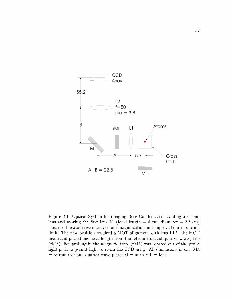
37
CCD
Array
L2
f=50
dia = 3.8
L1 Atoms
Glass
Cell
M�
A
B
55.2
5.7
rM�
A+B = 22.5
M
Figure 2.1: Optical System for imaging Bose Condensates. Adding a second
lens and moving the �rst lens L1 (focal length = 6 cm, diameter = 2.5 cm)
closer to the atoms we increased our magni�cation and improved our resolution
limit. The new position required a MOT alignment with lens L1 in the MOT
beam and placed one focal length from the retromirror and quarter-wave plate
(rM�). For probing in the magnetic trap, (rM�) was rotated out of the probe
light path to permit light to reach the CCD array. All dimensions in cm. M�
= retromirror and quarter-wave plate; M = mirror; L = lens.

38
2.4 Measurements of the Interaction Energy
The ballistic expansion we employed to facilitate imaging also gave us
a way to measure the mean energy of the cloud. When we suddenly turn o� the
trap potential, the harmonic oscillator energy EHO vanishes. By energy con-
servation, the kinetic energy plus the self interaction energy of the condensate
then appear in the form of purely kinetic energy E of the expanding cloud. By
varying the frequency of the trap and the number of atoms, we measured this
energy as a function of interaction strength. According to the virial theorem,
if the particles were ideal then E would equal half the total energy. However,
for a system with repulsive interactions the energy per particle due to Eint can
be non-negligible and E � 12Etot.
We approached the zero-temperature limit described by the Gross-
Pitaevskii Equation (eq.(2.1)) by evaporatively cooling to a point where the
non-condensate component was no longer observed, corresponding to T=T0 <
0:5 and N0=N > 0:8. Exact temperature and condensate fraction for these
deeply evaporated condensate clouds was di�cult to determine because no non-
condensate atoms were seen. We evaporated to BEC in the 373 Hz trap, then
adiabatically ramped the trap �elds to reach a new trap frequency and change
the strength of interaction in the condensate. We released the condensate
from this new trap by suddenly turning o� the magnetic �elds. In practice, a
weak magnetic trap remains which served to support the atoms against gravity
to allow longer expansion times. The e�ect of this remaining �eld on the
expansion was calculated as always less than 6% and was accounted for in the
analysis. We checked that our release of the atoms was purely non-adiabatic
by expanding uncondensed clouds, with T=T0 � 1:3 from di�erent frequency

39
traps. We observed that the expanded clouds are symmetric and found that,
for axial trap frequencies from 130 to 870 Hz, the energy expressed in units of
trap frequency, E=Nh�r, was constant to within 5%, as expected for classical
clouds in the non-interacting limit.
We performed expansions of condensates for the same range of trap
frequencies. In this experiment, each energy measurement consisted of typically
ten pictures of condensates taken for di�erent expansion times. We �t the
data twice, using the two di�erent limiting cases for the functional form - the
Gaussian of a non-interacting condensate and a parabolic surface for a strongly
interacting condensate in the TF limit. At short expansion times, the cloud
widths changed non-linearly with time as Eint was transformed into the pure
kinetic energy of the cloud. At long expansion times we performed a linear �t
to the expanded cloud widths to obtain the mean axial and radial velocities
(see inset to Fig.2.2), from which we calculated the total energy E.
Fig.2.2 contains condensate expansion data for N � 4200 (circles),
2100 (triangles), and 800 atoms (square) released from traps having axial fre-
quencies from 130 to 870 Hz. By using the product Np�r as the dependent
variable we combined our di�erent number and trap frequency data into one
�gure. From the trap asymmetry � =p8 the measured kinetic energy was
expected to be � 1:207. Note that the energies measured with parabolic �ts
for the most weakly interacting clouds were inconsistent with the energy in the
non-interacting limit. The parabolic surface �ts yielded lower energies than
the Gaussian �ts for all interaction strengths. We compared our measured
condensate energy, as a function of interaction strength, with the theoretical
prediction of Dalfovo and Stringari, who used the standard Gross-Pitaevskii
theory to calculate the energy of the condensate in the zero-temperature limit

40
Figure 2.2: We measured the condensate energy as a function of e�ective in-
teraction strength of Np�. The expansion velocity, and therefore energy, was
obtained from a linear �t to the time-dependent widths of freely expanding
condensates (inset). The widths were obtained from �ts to either a Gaus-
sian (solid shapes) or a parabolic surface (open shapes), as discussed in the
text. The condensates contained � 4200 (circles), � 2100 (triangles) or � 800
(squares) atoms. The solid line shows the mean �eld prediction by Dalfovo and
Stringari [5], which agrees well with the Gaussian �t data. Figure taken from
Ref.[6].

41
[5]. The solid line in Fig.2.2 shows the prediction using the current best value
of the scattering length for ground-state 87Rb atoms, a = 110a0, where a0 is
the Bohr radius [108, 131]. Unlike results presented by Mewes et al. [121],
the theory curve has no free parameters. Our energy data, measured from
Gaussian �ts, agrees reasonably well with the mean-�eld theory results.
2.5 Conclusions
Through several improvements in the original BEC apparatus we were
able to perform quantitative studies of the interaction energy present in Bose
condensates. For the data described here, Gaussian �ts to the expanded clouds
yielded condensate energies that are more in agreement with the predictions of
a Gross-Pitaevskii mean-�eld theory than �ts with paraboloids. Nonetheless,
even the condensate energies derived from Gaussian �ts are systematically
higher than the theory, for the largest interaction strengths. For the regime
of strong interactions, a parabolic surface should be a better approximation to
the condensate density. A quantitative reconciliation between our data and the
results of mean-�eld theory was achieved by Holland, et al. [7]. Using a mixed
distribution to �t the condensate, consisting of a central parabolic surface
and a Gaussian distribution in the periphery, they obtained good quantitative
agreement between the measured expansion energies and energies predicted
from mean-�eld theory (see Figure 2.3).

42
0 1 2 3 4 5 6 70
0.5
1
1.5
2
2.5
3
3.5
0 5 10 15 200
5
10
µm
)/ hε
ν
10
σ
N
Time (ms)
-4 ν1/2 [Hz1/2]
(
Figure 2.3: Comparison of the release energy as a function of interaction
strength from mean-�eld theory (solid line) and the experimental measure-
ments (�). Inset shows experimental widths in the horizontal (�) and vertical
(�) directions against the mean-�eld predictions (dashed and solid lines) for
the data point at 10�4N�1=2 = 0:53 Hz1=2. Used with permission of M. Holland
from Ref.[7].
Chapter 3
Collective Excitations of a Bose-Einstein Condensate in a Dilute
Gas
3.1 Introduction
Early experiments with BEC showed that interatomic interactions
in uence the energy and wavefunction of a zero-temperature condensate [121,
6]. Using simple Gaussian or paraboloid models of the density distribution of
the condensate, we observed good qualitative agreement between our energy
data and the predictions of the Gross-Pitaevskii mean-�eld theory [124, 125,
126]. Unfortunately, the model pro�les �t the subtle features of the condensate
pro�le too crudely, and thereby compromised a quantitative and detailed test
of theory. Gross-Pitaevskii theory also makes predictions for the existence
of elementary condensate excitations [9, 10, 11, 12, 134, 135]. Such time-
dependent behaviour was more amenable to a precise measurement since it
was easier to measure a frequency accurately than to determine the absolute
features of the density pro�le. We report herein on studies of low-energy,
collective excitations of a dilute condensate of 87Rb. Characterizing these low-
lying excitations was a �rst step towards understanding the dynamics of this
novel quantum uid [136].

44
3.2 Experimental Procedure
The apparatus and procedures for creating and observing BEC were
the same as used in Section 2.3. For the experiments described here, the �nal
evaporation took place in a trap with a radial frequency of 132 Hz (373 Hz
axial). To approach the zero-temperature limit, we evaporated well below the
BEC phase transition [137] so that the expanded clouds showed no sign of hav-
ing a thermal component. At higher temperatures, this component appeared
as a broad, symmetric Gaussian background [22]. Typically we had 4500�300
atoms in the condensate.
3.3 Theory of Excitations
The standard theory for BEC in a dilute atomic vapor uses a non-
linear Schr�odinger equation, the Gross-Pitaevskii equation, to describe the con-
densate wavefunction in the limit of zero temperature [138]. This equation
comes from a second-quantized mean-�eld theory with the interatomic inter-
actions modeled by an s-wave scattering length. The elementary excitations of
BEC in a �nite, harmonically-con�ned dilute gas were studied theoretically us-
ing this model [9, 10, 11, 12, 134, 135]. The lowest energy normal modes of the
condensate, corresponding to rigid-body center-of-mass motion (\sloshing"),
were predicted to occur at the trap frequencies. The frequencies of the next
lowest condensate excitation modes, however, were expected to deviate from
the spectrum of a cloud of ideal gas, for which the excitation frequencies are
simply multiples of trap frequencies. Not surprisingly, the amount of deviation
depends on the strength of the interatomic interactions.
45
3.4 Exciting collective modes
We excited these collective modes of the condensate by applying a
small time-dependent perturbation to the transverse trap potential. We gener-
ated the perturbations by applying a sinusoidal current to the coils responsible
for the rotating �eld of our TOP trap (in addition to the normal TOP cur-
rents). The response of the condensate depends on the symmetry of the driving
force as well as the driving frequency, �d. By appropriately setting the phases
of the currents through the coils, we generated perturbations with either of
two di�erent symmetries. We label these two driving symmetries m = 0 and
m = 2, where m, the angular momentum projection onto z, is a good quan-
tum number because of the axial symmetry of our unperturbed magnetic trap.
Equipotential contours for the two trap perturbations are shown in Fig. 3.1.
The m = 0 drive preserved axial symmetry and corresponds to an oscillation
in radial size. For the m = 2 drive symmetry, the trap spring constants along x
and y were modulated 90� out of phase. This corresponded to a normal mode
resembling a transverse ellipse whose major axis rotates in the x� y plane.
The basic spectroscopic approach was as follows: we distorted the
cloud by applying the perturbative drive for a short time, then allowed the
cloud to evolve freely in the unperturbed trap for a variable length of time.
Finally, we turned o� the con�ning potential suddenly and imaged the resulting
cloud shape after 7 ms of free expansion.
3.5 Observation of Excitations
Initial studies were made in a 132 Hz trap. The perturbative drive
pulse duration was 50 ms, the center frequency was set to match the frequency

46
Figure 3.1: In the unperturbed trap, contours of equipotential in the transverse
plane are symmetric (solid line). To drive them = 0 excitation (a) we applied a
weak harmonic modulation with frequency �d to the trap radial spring constant.
The m = 2 drive (b) broke axial symmetry with elliptical contours which rotate
at �d=2. The amplitude of perturbation is shown exaggerated for clarity. Figure
taken from Ref.[8].

47
of the excitation being studied, and the amplitude was 1.5% of the radial spring
constant of our trap. We observed two di�erent collective excitations of the
condensate. The observables in both cases were the widths of the expanded
clouds as a function of the free evolution time. In one case we observed a
sinusoidal oscillation of the radial width at a frequency of (1:84�0:01)�r, where
�r is the radial trap frequency and the error quoted re ects only statistical
uncertainties. This mode was driven by the axially symmetric m = 0 trap
perturbation and was not observed for the drive with m = 2 symmetry (with
the same drive amplitude and frequency). The cloud widths oscillated in both
axial and radial directions, with approximately opposite phase. This response
is shown in Fig. 3.2. The observed phase di�erence between the oscillations
of axial and radial widths is not exactly �; however, the free expansion of the
condensate prior to imaging complicates analysis of this phase shift [139]. The
second excitation oscillated freely at (1:43� 0:01)�r, and appeared in response
to a m = 2 drive, and not to a m = 0 drive. In this case, the radial width
oscillated, with no observable response in the axial width. The two-dimensional
projection of an ellipsoidal cloud whose major axis rotates in the transverse
plane would exhibit this behavior.
We calibrated the observed excitation frequencies in units of the trap
frequencies by making similar measurements on non-condensate clouds. The
temperature of these clouds, in units of the BEC transition temperature, is
T=Tc � 1:3; consequently the density and thus the interactions were very
small. Here, we saw a response that oscillated at 264 Hz and was driven with
either symmetry. A harmonically con�ned, noninteracting gas pulses at twice
the radial trap frequency, so this gave �r = 132� 1 Hz. We also checked that
the thermal cloud did not respond when driven at 1:43�r.

48
3.6 E�ect of Interactions
In the s-wave scattering approximation, the interactions for ground
state 87Rb atoms in our trap are repulsive (positive scattering length) [108, 131],
providing an e�ective potential energy which favors a lower central density of
the condensate compared to the non-interacting case. This interaction energy
determines the excitation spectrum of the condensate [140]. We were able to
examine this e�ect because BEC in trapped neutral atoms o�ers the advantage
of an adjustable interaction energy. In the standard mean-�eld picture, the
strength of the non-linear interaction term in the Gross-Pitaevskii equation,
relative to the harmonic trap's energy-level spacing, scales with Nap�r for the
regime of interactions in which the ground-state density is well-approximated
by a Gaussian [128, 129, 130, 5]. Thus, by varying the trap frequency or the
number of atoms, N , we changed the relative importance of interactions in the
condensates.
We measured the excitation frequencies of the m = 0 and m = 2
modes of the condensate as a function of both N and �r. In the 132 Hz trap,
we changed the relative interaction strength by reducing the number of atoms.
To change �r, we evaporated to BEC in the 132 Hz trap, then adiabatically
ramped the trap �elds until the condensate was held in a trap with an axial
frequency of 43.2 Hz. In this lower frequency trap, we excite the condensate
with a 100 ms pulse and a drive amplitude equal to 3% of the radial spring
constant. The observed fractional amplitude of the oscillations in the cloud
width was typically 11% of the mean width for this drive. We measured the
free oscillation frequency of the m = 0 and m = 2 modes in this trap to be
(1:90� 0:01)�r and (1:51� 0:01)�r, respectively, for N � 3000.

49
5 10 15 2012
14
16
18
24
26
28
30
radial axial
FW
HM
(µ m
)
time (ms)
Figure 3.2: We applied a weak m = 0 drive to a N � 4500 condensate in a
132 Hz (radial) trap. Afterward, the freely evolving response of the condensate
showed radial oscillations. Also observed is a sympathetic response of the axial
width, approximately 180� out of phase. The frequency of the excitation was
determined from a sine wave �t to the freely oscillating cloud widths. Each
data point represents a single destructive condensate measurement. Figure
taken from Ref.[8].

50
The measured excitation frequencies as a function of interaction stren-
gth are shown in Fig. 3.3. By using the product Np�r for the dependent
variable we combine our di�erent number and trap frequency data into one
graph. The solid lines in Fig. 3.3 show the mean-�eld theory calculation by
Edwards et al. [9, 10], using the best value of the scattering length for ground
state 87Rb atoms available at the time, a = 110ao [108], where ao is the Bohr
radius. An extension of this calculation by Esry and Greene is shown with
dotted lines [11]. Finally, dashed lines indicate the prediction by Stringari for
the \strongly interacting" limit [12], in which the kinetic energy of the ground
state is ignored. Our data agreed reasonably well with these mean-�eld theory
results; the measured energies of the low-lying collective excitations of the
condensate deviate from the simple harmonic trap spectrum as predicted, with
larger deviation for larger interaction strength. Error bars in Fig.3.3 indicate
statistical error in the determination of the frequencies, but do not include
possible systematic errors such as day-to-day variations in the trap magnetic
�elds, and therefore frequencies (estimated to be less than 0:5%). A signi�cant
systematic also arose from our method of using the m = 0 non-condensate
mode to calibrate the trap frequency: Measurements of �nite temperature
excitations [141] indicated this caused our measured excitation frequencies to
be low by 1%. Also, the theoretical curves are strictly valid only in the limit
of zero temperature and zero amplitude.
In the limit of low excitation amplitude, the spectrum of low-lying col-
lective excitations corresponds exactly to the Bogoliubov quasi-particle spec-
trum [9, 10]. The collective condensate response to our trap perturbation,
in the limit of low amplitude, is simply a coherent state of these elementary
excitations. To explore the question of whether or not our experiments were

51
0 2 4 61.2
1.4
1.6
1.8
2.0
10-4 N νr1/2
ν / ν
r
Figure 3.3: We measured the frequency of the m = 0 (triangles) and m = 2
(circles) condensate modes as a function of interaction strength. The relative
interaction strength in the condensate varied as the product of number of
atoms, N , and the square root of the radial trap frequency, �r. Solid lines
show the mean-�eld calculation by Edwards and co-workers [9, 10], dotted
lines show the results of similar calculations by B. Esry and C. Greene [11] and
dashed lines show the prediction by Stringari for the strongly-interacting limit
[12]. Figure taken from Ref.[8].

52
performed in this limit, we measured the condensate response for di�erent driv-
ing force amplitudes. In this test, we drove the m = 2 mode in the 132 Hz trap,
with N � 4500. The results are shown in Fig. 3.4 where we plot the frequency
of the oscillating radial width as a function of the amplitude of that response.
The solid line shows a �t to a parabola, a form which describes an oscillator
with anharmonic terms. As our measurements of excitation frequency were
performed for a response amplitude between 9 and 14%, which caused a shift
of only 1% in the frequency, this data suggests that we are in the regime where
the measured spectrum corresponds quite closely to the elementary excitations
of BEC in a dilute gas.
3.7 Damping
Finally, we examined the damping of a condensate excitation. For
comparison purposes we �rst studied the damping in a noncondensed thermal
cloud (T=Tc � 1:3) in the 132 Hz trap. We excited the 264 Hz m = 0 mode,
because damping in this mode is not in uenced by angular momentum con-
servation. We �t a sine wave with an exponentially decaying amplitude to the
observed oscillations in the radial cloud width. This gave an excitation lifetime
of 49 � 13 ms. Since the mean free path in these clouds is long compared to
the excitation wavelength and the e�ect of the trap anharmonicity is small, the
excitation lifetime should scale inversely as the atom-atom collision rate. This
rate in turn scales with the product of the density times the velocity of the
atoms. For a given harmonic oscillator con�ning potential, this collision rate is
proportional to the optical depth of the cloud. Using this scaling principle we
predicted that the damping lifetime in a classical cloud with the same optical

53
0 20 40 60180
190
200
210
220
m=2 excitation
Fre
quen
cy (
Hz)
Amplitude (%)
Figure 3.4: The freely oscillating frequency of the condensate is shown as a
function of response amplitude. The condensates, consisting of 4500 atoms,
were held in a 132 Hz radial frequency trap and driven with m = 2 symmetry.
The solid line shows a parabolic �t to the data. Figure taken from Ref.[8].

54
depth as the condensate would be 28� 8 ms.
But when we performed the same experiment on the 4500 atom con-
densate we obtained an excitation lifetime of 110�25 ms. Thus, the condensate
excitation persisted nearly four times longer than can be explained in a classical
picture.
In summary, we observed low-lying collective excitations of BEC in a
dilute atomic vapor. Both m = 0 and m = 2 modes were identi�ed, and their
frequencies measured as a function of relative interaction strength. The data
were taken in a linear regime where the collective modes should correspond to
the elementary excitations of BEC in this system, and reasonable agreement
was found between the experiment and mean-�eld theory results. The damping
lifetime of the m = 0 excitation was measured and found to be signi�cantly
longer than the prediction of a classical model. We believe further study of
these elementary excitations, particularly at di�erent temperatures, will help
deepen the understanding of the quantum phenomena of Bose-Einstein con-
densation of a gas.

Chapter 4
Bose-Einstein Condensation in a Dilute Gas: Measurement of
Energy and Ground-State Occupation
4.1 Introduction
The ability to create Bose-Einstein condensation (BEC) in magnet-
ically trapped alkali gases [22, 119, 142, 122] provided an opportunity to ex-
perimentally study the thermodynamics of bosonic systems in which the inter-
actions are (i) weak, (ii) binary and (iii) experimentally adjustable [8, 121, 6].
One goal of experimental and theoretical work in this �eld was to understand a
variety of low-temperature phenomena from both macroscopic and microscopic
points-of-view, with a quantitative reconciliation of these two approaches. The
experimental studies of collective excitations of zero-temperature condensates
( [8, 143] and Chap. 3). were a step in this direction. The purpose of the
present chapter is to explore the nature of the BEC phase transition by per-
forming quantitative measurements of BEC in a di�erent regime { near the
critical temperature [144].
In this chapter we analyze a series of images of ultra-cold clouds of
rubidium gas to determine the critical temperature and to extract ground-
state occupation and total energy as a function of temperature. Total energy
(or its derivative, speci�c heat) has a certain historical signi�cance because it

56
was Fritz London's comparison [38] of the speci�c heats of liquid helium and
an ideal Bose gas that began the rehabilitation of BEC as a useful physical
concept. Moreover, measurements of thermodynamic quantities such as speci�c
heat are essential in studying any phase transition. Ground-state occupation
and critical temperature of a Bose gas are interesting because in liquid helium
the former is very di�cult to measure, while the latter is almost impossible to
calculate accurately.
4.2 Experiment
The apparatus and procedures for creating BEC were the same as
used in Sections 2.3 and 3.2. The imaging procedure used here di�ers in two
speci�c ways. First, the atoms were always allowed to expand freely for a time
of 10 ms before probing by the resonant probe beam. Secondly, we applied
point-by-point corrections for imperfect polarization and saturation e�ects in
our digital analysis to render the true 2-d projection of the velocity distribution
in the expanded cloud.
4.3 Data Analysis
These distributions contain a wealth of thermodynamic information.
For instance, the integrated area under the distribution is proportional to the
total number, N , of atoms in the sample. The condensate appears as a narrow
feature centered on zero velocity [22]; the number of atoms in the ground state,
No, is then proportional to the integrated area under this feature. From the
mean square radius of the expanded cloud and the expansion time, we get the
mean square velocity, or average energy, of the cloud. Finally, as discussed

57
below, the temperature, T , is extracted from the images, even though the
temperature is not merely proportional to mean energy in a degenerate Bose
cloud.
We went to some lengths to extract these thermodynamic quantities
in a model-independent way. For instance, if we were to �t the observed veloc-
ity distributions to a Bose-Einstein distribution, we could hardly avoid coming
to the conclusion that the speci�c heat is discontinuous - the singular behavior
is built-in to the assumed functional form. Moreover, such a �t would preclude
our being able to observe e�ects due to interactions, �nite N , critical uctu-
ations, etc. Fortunately, useful thermodynamic information about the sample
can be extracted from direct calculation of various moments of the velocity
distribution, without speci�c reference to the nature of the distribution. The
total number and energy of the atoms, as mentioned above, are simply propor-
tional to the zeroth and second moments, respectively, calculated directly by
summing over the velocity distribution images [145].
We de�ned the number of atoms in the ground state to be the number
of atoms contributing to the narrow, central feature in the optical depth images
[22]. To avoid biased and noisy results we provided the least-squares �tting
routine with a tightly constrained template to use in its search for a condensate.
With an independent set of measurements on condensates near zero temper-
ature, we found that the condensate shapes were well-�t with 2-d Gaussians
whose widths, aspect ratios and peak-heights, for a given trap frequency and
expansion time, were functions only of the total number of atoms in the fea-
ture [6, 7]. The width, for instance, was parameterized by � = �o(1+�No)1=5,
where �o is the predicted non-interacting condensate width and � was extracted
empirically. The procedure yielded robust values of No, as long as the temper-

58
ature was high enough that the non-condensate atoms formed a distribution
that was signi�cantly broader than the sharp condensate feature. At tempera-
tures below T=To = 0:5, both T and No measurements became suspect as it was
no longer possible to cleanly separate the condensate and the non-condensate
components without recourse to a detailed model, which was contrary to the
spirit of this treatment.
Our thermometry di�ered from previously reported methods for ultra-
cold trapped gases [22, 119, 142, 8, 121, 6, 143]. For an ideal gas far from
quantum degeneracy the velocity distribution is a Gaussian whose width is
proportional to T 1=2. As the cloud is cooled closer to the BEC phase transition,
higher densities and lower temperatures cause a rapid increase in the signif-
icance of quantum statistics and of residual atom-atom interactions. Rather
than attempt to model these e�ects, we assumed that the high-energy tail
of the velocity distribution (i) remained in thermal equilibrium with the rest
of the cloud and (ii) was characterized by a purely ideal Maxwell-Boltzmann
(MB) distribution. The latter is plausible because these highest energy atoms
spend most of their trajectories in the low-density, and therefore weakly inter-
acting, outer part of the trapped cloud. Furthermore, the occupation numbers
of the corresponding energy states are much less than one. Finally, during the
free expansion, the high-energy atoms underwent on average much less than
one collision. Guided by these assumptions, we determined the temperature
by �tting a 2-d Gaussian to only the wings of our velocity-distribution images,
excluding the central part of the cloud, where degeneracy, interactions, uctu-
ations, etc. may be signi�cant. To test the assumption of thermal equilibrium
we checked that the measured temperature of clouds were independent of the
size of the exclusion region, outside of the degenerate regime [146].

59
0.0 0.5 1.0 1.5
0.0
0.2
0.4
0.6
0.8
1.0
No/
N
T / To (N)
0.0 0.5 1.0 1.5
4
8
12
N (
104 )
Figure 4.1: Total number N (inset) and ground-state fraction No=N as a func-
tion of scaled temperature T=To. The scale temperature To(N) is the predicted
critical temperature, in the thermodynamic (in�nite N) limit, for an ideal gas
in a harmonic potential. The solid (dotted) line shows the in�nite (�nite)
N theory curves. At the transition, the cloud consisted of 40,000 atoms at
280 nK. The dashed line is a least-squares �t to the form No=N = 1� (T=Tc)3
which gives Tc = 0:94(5)To. Each point represents the average of three separate
images. Figure taken from Ref.[13].

60
4.4 Ground-State Fraction
The �rst quantity we examined is the ground-state fraction, No=N ,
as a function of scaled temperature T=To (Fig. 4.1). The temperature scaling
removed the trivial shift in the transition temperature which occurred because
as we evaporatively cool through the transition we also reduced the total num-
ber of atoms, N (Fig. 4.1, inset). We chose our scaling temperature to be
To(N) = ~�!=kB(N=�(3))1=3 where �! is the geometric mean of the trap frequen-
cies and � is the Riemann Zeta function. To(N) is also the critical temperature,
in the thermodynamic limit, for non-interacting bosons in a harmonic poten-
tial [147, 84]. For this case the temperature dependence of the ground-state
fraction is No=N = 1� (T=To)3 below To (solid line, Fig. 4.1). We emphasize
that, in contrast with the recent work of Mewes et al. [121], this line contains
no free parameters and was not �t to the data, and so comparing this line to
our data provides a detailed test of theory.
From our data we found a critical temperature of Tc = 0:94(5)To.
The uncertainty was dominated by the systematic uncertainty in our measure-
ment of the scaled temperature stemming mostly from a 2% uncertainty in
the magni�cation of our imaging system. Our measurements were thus only
marginally di�erent from the theory for non-interacting bosons in the ther-
modynamic limit. Finite-number corrections [14, 15] will shift the transition
temperature Tc(N) down about 3% (dotted line, Fig. 4.1). Mean-�eld [84, 148]
and many-body [149] interaction e�ects may also shift Tc(N) a few percent.

61
4.5 Energy
The second result we present is a measurement of the energy and
speci�c heat. Ballistic expansion, which facilitates quantitative imaging, also
provided a way to measure the energy of a Bose gas [121, 6, 8]. The total energy
per particle of the trapped cloud consists of harmonic potential, kinetic, and
interaction potential energy contributions, or Epot, Ekin and Eint, respectively.
As the trapping �eld was non-adiabatically turned-o� to initiate the expansion,
Epot suddenly vanished. During the ensuing expansion, the remaining compo-
nents of the energy, Ekin and Eint, were then transformed into purely kinetic
energy, E, of the expanding cloud: Ekin + Eint ! E, where E is the quantity
we actually measured. According to the virial theorem, if the particles are ideal
(Eint = 0), E will equal half the total energy, i.e. E = 1=2Eidealtot . However, for
a system with interparticle interactions the energy per particle due to Eint can
be non-negligible and then E = �Etot, where � is not necessarily 1=2.
The scaled energy per particle, E=NkBTo, is plotted versus the scaled
temperature, T=To, in Fig. 4.2. E=N was normalized by the characteristic
energy of the transition kBTo(N) just as the temperature was normalized by To.
The data shown were extracted from the same cloud images as those analyzed
for the ground-state fraction. Above To, the data tended to the straight solid
line which corresponded to the classical MB limit for the kinetic energy. Most
interesting was the behavior of the gas at the transition. By examining the
deviation, �, of the data from the classical line we saw (Fig. 4.2, inset) that the
energy curve clearly changed slope near the empirical transition temperature
(0:94To) obtained from the ground-state fraction analysis discussed above.

62
0.4 0.6 0.8 1.0 1.2 1.4 1.6 1.80.0
0.5
1.0
1.5
2.0
∆E /
Nk B
To
T / To(N)
0.4 0.8 1.2 1.6
-0.4
-0.2
0.0
Figure 4.2: The scaled energy per particle E=NkBTo of the Bose gas is plotted
vs. scaled temperature T=To. The straight, solid line is the energy for a classi-
cal, ideal gas, and the dashed line is the predicted energy for a �nite number
of non-interacting bosons [14, 15]. The solid, curved lines are separate poly-
nomial �ts to the data above and below the empirical transition temperature
of 0:94To. (inset) The di�erence � between the data and the classical energy
emphasizes the change in slope of the measured energy-temperature curve near
0:94To (vertical dashed line). Figure taken from Ref.[13].

63
4.6 Speci�c Heat
The speci�c heat is usually de�ned as the temperature derivative of
the energy per particle, taken with either pressure or volume held constant. In
our case the derivative was the slope of the scaled energy vs. temperature plot
(Fig. 4.2), with neither pressure nor volume, but rather con�ning potential
held constant. To place our measurement in context, it is instructive to look
at the expected behavior of related speci�c heat versus temperature plots (Fig.
4.3). The speci�c heat of an ideal classical gas (MB statistics), displayed as
a dashed line, is independent of temperature all the way to zero temperature.
Ideal bosons con�ned in a 3-d box have a cusp in their speci�c heat at the
critical temperature (dotted line) [38]. Liquid 4He can be modeled as bosons
in a 3-d box, but the true behavior is quite di�erent from an ideal gas, as
illustrated by the speci�c heat data [16, 17] (dot-dash line): the critical (or
lambda) temperature is too low, and the gentle ideal gas cusp is replaced by
a logarithmic divergence. We compared our data with the calculated speci�c
heat of ideal bosons in a 3-d anisotropic simple harmonic oscillator (SHO)
potential [147] (solid line). Note that because we did not measure Epot, we
had to divide the SHO theory values by two to compare with our measured
expansion energies. The speci�c heat of the ideal gas is discontinuous and �nite
at the transition.
In order to extract a speci�c heat from our noisy data, we assumed
that, as predicted, there was a discontinuity in the slope at the empirically
determined transition temperature and �t the data to separate polynomials on
either side of Tc (curved, solid lines in Fig. 4.2). We extracted the speci�c heat
curve shown in Fig. 4.3 (bold line in inset). The observed step in the speci�c

64
heat at the critical temperature was considerably smaller than predicted by a
�nite number, ideal gas theory [14, 15] (Fig. 4.3, inset, thin line). A more
sensible comparison is to avoid taking the model-dependent derivative and
instead to compare theory and experiment directly in the energy-temperature
plot (Fig. 4.2). The major deviation between the data and the SHO ideal
gas theory (dotted line) occurs at scaled temperatures of 0.85 and below. The
di�erence is probably due in part to the e�ects of interactions. Mean-�eld
repulsion will tend to increase the energy at a given temperature.
4.7 Summary and Epilogue
We measured the critical temperature, ground-state occupation and
energy of a dilute Bose gas of 87Rb atoms. Our analysis was unique in that it
did not rely on detailed models of the quantum degenerate cloud shape. We
were thus able to examine the thermodynamics of the Bose gas in an unbi-
ased and quantitative way. The measured ground-state fraction and transition
temperature agreed well with the theory for non-interacting bosons. However,
the qualitative features of the energy data are signi�cantly di�erent from the
non-interacting theory.
Recent theoretical results [18, 150, 151] that consider the e�ects of
mean-�eld interactions at �nite temperature are in good agreement with our
data. The theories adapt the standard Gross-Pitaevskii treatment [129, 5] to
include the condensed and non-condensed components of the gas. Generally,
mean-�eld interactions reduce the ground-state occupation and increase the
energy per particle compared to the non-interacting Bose gas (in the thermo-
dynamic limit) at the same temperature. A downward shift in the critical

65
0.6 0.8 1.0 1.2 1.40
1
2
3
4
5
63d SHO
3d box
4He data
C /
Nk B
T / To(N)
0.8 1.0 1.20
2
4
Figure 4.3: Speci�c heat, at constant external potential, vs. scaled temperature
T=To is plotted for various theories and experiment: theoretical curves for
bosons in a anisotropic 3-d harmonic oscillator and a 3-d square well potential,
and the data curve for liquid 4He [16, 17]. The at dashed line is the speci�c
heat for a classical ideal gas. (inset) The derivative (bold line) of the polynomial
�ts to our energy data is compared to the predicted speci�c heat (�ne line)
for a �nite number of ideal bosons in a harmonic potential. Figure taken from
Ref.[13].

66
temperature due to �nite number and mean-�eld is also predicted. Our data
for the ground-state occupation lie between the mean-�eld predictions and the
ideal gas model [18, 151]. Due to systematic uncertainties in our temperature
measurement, the di�erences between our measurements and the recent the-
ory are marginal, however. The predicted energy per particle is in excellent
agreement with our measurements (Figure 4.4), including the observation of a
feature in the speci�c heat.
In future work we will attempt to elucidate the role interactions play
in the phase transition and the speci�c heat. For example, we can control
the interactions by adjusting the magnetic trap spring constants and changing
the number of trapped atoms [8]. In addition, with larger clouds [122] we
can reduce our uncertainty in Tc, allowing us to investigate �nite-number and
mean-�eld e�ects at the 1% level.

67
Figure 4.4: The sum of kinetic and interaction energy, as de�ned in the [18],
obtained in the two- uid model, compared with the data of Ensher et al [13]
(diamonds) and with the ideal gas result (dotted curve). Results obtained from
the zero-order solution (full curve), from the �rst-order perturbative treatment
(dashed curve) and from the complete numerical solution (circles). The straight
line is the classical Maxwell-Boltzmann result. The inset is an enlargement of
the region around Tc. Figure taken from Ref.[18] with permission of S. Conti.

Chapter 5
The Third Generation BEC Machine at JILA
In this chapter I describe the latest and most sophisticated apparatus
constructed at JILA to quickly (1 � 1:5 min) produce large BECs (typically
106 atoms). The chapter focuses on experimental details ranging from funda-
mental design considerations to actual experimental conditions. The apparatus
uses a double-MOT system to quickly load a purely magnetic trap in a low-
background pressure environment, in which radio-frequency (rf) evaporative
cooling is performed to reach BEC. I begin with a description of our vacuum
system, followed by discussion of the Collection MOT (Magneto-Optical Trap),
the Science MOT and the transfer of atoms from Collection MOT to Science
MOT. Next, I discuss construction of the TOP magnetic trap, transfer from
the Science MOT into the TOP magnetic trap and rf evaporation. The chapter
concludes with a description of the absorption imaging system.
5.1 Vacuum System
The heart of the BEC apparatus is the double-MOT vacuum design
�rst implemented by Myatt, et al. [93, 152]. The system uses a glass cell
maintained at 10�9 Torr of Rb for rapid loading of a MOT with many atoms
(� 108 atoms in 1�2 sec). We refer to this as the Collection Cell and the MOT

69
it contains as the Collection MOT. A long transfer tube connects the Collection
cell to a second glass cell maintained at much lower pressure (10�11 � 10�12
Torr). The low-pressure cell, which we refer to as the Science Cell, allows
long MOT and magnetic trap lifetimes. The Science cell is also designed for
small magnetic �eld coils that create a high-con�nement magnetic trap with
minimized power dissipation. Finally, many windows with optical-quality glass
allow for excellent access to the atoms in the Science Cell.
5.1.1 The Collection Cell
The collection cell is designed to collect a large number of atoms into
a MOT simply and quickly. Two features are essential for rapid loading of the
MOT with many atoms: large beam size and large amounts of trap light [153].
The high power laser used for trapping will be discussed in Section 5.2.1. The
Collection cell accommodates large trap beams with six, 35 mm dia windows
that provide access along each cardinal direction (Figure 5.1). Even larger
windows would be bene�cial, but the cost is a loss of simplicity. A larger glass
cell requires larger coils and more amp-turns for the quadrupole potential of the
MOT and the magnetic shim �elds. At the present coil sizes, we supply enough
current with simple 30V, 6A power supplies using air-cooled coils made from
magnet wire. There is little heating of the glass due to the power dissipated
from the coils. Another trade-o� with large volume is the need for greater
pump speeds.
Two other features of the Collection cell are worth noting. First, there
are three, 10 mm diameter viewing windows. Two windows, facing opposite
each other and perpendicular to the transfer tube axis, are used for monitoring
atoms with a charged-coupled device (CCD) camera and a photodiode (PD).

70
The third window faces down the transfer tube and permits a laser pulse to push
the MOT atoms down the tube. The second feature is the Rb metal dispenser
used as a low-maintenance, high- ux source of atoms. Three dispensers are
installed in each of two glass arms with vacuum feedthroughs, made of wire,
leading to the dispensers. The dispensers emit Rb atoms, as discussed in
Section 5.1.7.
5.1.2 The Science Cell
The Science cell (Fig.5.2) holds a large MOT of > 109 atoms, which
we refer to as the Science MOT, yet is compact enough to keep magnetic �eld
coils close to the atoms for high-con�nement magnetic trapping. There are �ve
main features of the Science Cell. (i) Six, 2:5 cm dia windows of good quality
permit up to 2:5 cm dia MOT beams, which is necessary to contain a large
number of atoms in the MOT. (ii) A \2-d" design of the cell, such that the
cell is compact in the vertical direction, permits placement of quadrupole coils
very near the atoms (for high magnetic �eld gradients). The small distance
between cell windows in the horizontal directions provides more clear angles to
the atoms and permits placement of the TOP coils nearer the atoms (for large
magnetic �elds). (iii) Three, 1 cm dia, high-quality windows in the horizontal
plane permit clean optical probing and monitoring. One window, facing down
the transfer tube, was initially used to align atom transfer and presently is used
for a monitor PD. The other two windows, facing perpendicular to the axis of
the transfer tube, are used for optically imaging the atoms. These latter two
windows are 3.5 cm away from the atoms and create a window-de�ned f=# of
3.5. (iv) The glass arm that connects the Science cell to the transfer tube has
two features. The length of the tube allows the main trap volume, at the center

71
To Vacuum Pump
Rb Dispensers
To ScienceCell
PushWindow
View Window(1 of 2)
MOTWindow(1 of 6)
Figure
5.1:Schem
atic
oftheCollectio
nCell

72
of the large windows, to be far away from the magnetic �elds of the transfer
tube. The bellows-to-con at connection reduces stress on the long glass arm
and permits some degree of freedom in the construction of the vacuum system.
(v) The 2:5 cm dia glass arm, which connects the Science cell to the large
vacuum assembly, maintains a relatively high conductance path to the vacuum
pump and the window at its end permits entry of one of the MOT beams
into the cell. The length of the arm strikes a compromise between structural
stability and the need to keep the vacuum apparatus away from the glass cell
for more convenient placement of optics.
5.1.3 Transfer Tube
The transfer tube is a 37 cm long, 1:3 cm dia stainless steel tube that
connects the Science cell to the Collection cell. Because the tube possesses a
conductance of only 0:5 L/sec it maintains a large (� 20�) di�erential pressure
between chambers while allowing atoms to be optically pushed from Collection
MOT to Science MOT. Near the Collection MOT, a short section of tube
branches o� the main transfer tube and connects the Collection cell to a 20
L/sec ion pump. Just beyond this branch is another short tube branch that
contains a glass-encased magnet (the glass capsule is � 3 � 4 cm long). The
magnet can be moved from outside the vacuum, using a solenoid, to obstruct
the tube and e�ectively \valve-o�" the two vacuum chambers. Along the entire
length of the tube we inserted a spiral-wound wire that rests against the inside
wall. The wire prevents shallow-angle scattering of light down the tube from
the Collection MOT light, which would limit transfer e�ciency by optically
depumping the atoms from a magnetically trapped transfer state.

73
To VacuumPumps
To CollectionCell
Imaging Window
MOT Window(1 of 6)
Figure 5.2: Schematic of the Science Cell
74
5.1.4 Pumps
We maintain sustained di�erential pressures between the Collection
MOT and the Science MOT with two ion pumps on either end of the transfer
tube. At the Collection cell end, we use a 20 L/sec ion pump that is actually
overkill given the limited conductance to the Collection cell. The e�ective
pump speed, at the cell, is only a few L/sec and the resulting pressure is of order
10�9 Torr. On the Science cell end, we are very concerned about maintaining
high vacuum so we use a 30 L/sec ion pump and Titanium Sublimation Pump
(TSP). The pumps are contained in a 4-way stainless-steel cross that is separate
from the Science cell. The arms of the cross are 6.4 cm dia and provide a large
surface area over which Titanium is periodically coated using sublimation from
the TSP �laments. The entire cross is hence a passive ion pump. The large
diameter arms also create a high conductance path from the 30 L/sec active
ion pump to the glass cell for an e�ective pump speed at the cell of about 10
L/sec. On the fourth arm of the cross a bakeable mechanical valve is attached
for the initial rough pump-down of the system and future vacuum servicing.
We make one �nal note concerning the pumps. Ion pumps use large
permanent magnets that generate substantial stray magnetic �elds. We pur-
posefully place the 30 L/sec pump as far from the Science cell as practical
without limiting the pump speed. We observe little e�ect on the atoms in the
Science MOT from this pump. Unfortunately, the 20 L/sec pump is placed
very near the Collection MOT, since it's e�ective pump speed is limited by
tube conductance. The stray �elds are a nuisance for the Collection MOT, as
they require larger shim coils that dissipate more heat.

75
5.1.5 System Layout
Several key ideas are incorporated into the layout:
�Minimize overall size to leave room on optical table for lasers, optics and
cameras
�Place cells near table edges for easy access to optics and coils
�Set cell heights consistent with standard height of the lasers on the table.
Keep the lasers mostly in one plane for eye safety.
�Preserve optical access by limiting obstruction by pumps and cells
�Design space for extensive light ba�es and shields.
�Place system on a separate breadboard to construct and bake the system away
from optics and lasers [154].
�Create thermal isolation between the vacuum system and the table for high
temperature bake-outs.
The overall layout of the double MOT is very compact, as it requires
a minimum of large and costly vacuum components (Figure 5.3). The system
occupies only 86 cm � 60 cm on the table. The absence of large and heavy
components means that the entire system is mounted simply on an optical
breadboard using only aluminum supports under the heaviest and most sen-
sitive joints. At the Collection cell end, the system is supported by holding
the 20 L/sec pump. At the Science cell end, the four-way cross is supported
under each arm by aluminum stands. The heavy 30 L/sec pump is supported
in part by its connection to the cross, and also by a stand under its neck near
the con at joint. In each of the ion pump mounts we allow for removal of
the permanent magnets (for baking the vacuum system and the pumps them-
selves). Finally, we support the con at joint where the Science cell meets the

76
transfer tube to prevent accidental breakage of the fragile glass tube. Under
all the mounts we place glass sheets or microscope slides to thermally isolate
the aluminum mounts from the breadboard.
5.1.6 Construction, Pump-down and Bake-out
Before construction of the vacuum system all the pieces, except the
ion pumps and cells, are degreased, cleaned in two ultrasonic baths, rinsed
with methanol and �nally rinsed with deionized water and left to air dry. The
stainless components are then baked in air at 400 �C for 3 hours to purge water
from the surfaces and form an oxide layer to bind surface sites where water
may adhere. The system is constructed with UHV clean protocol. An impor-
tant detail is we use non-magnetic and silvered screws in the con at joints.
The non-magnetic screws minimize stray magnetic �elds near our atoms. The
silvering allows us to use very little anti-seizing compound, greatly simplifying
and sanitizing the construction. Once built, we pump down and bake-out the
system using a grease and oil-free rough pumping station. The permanently
attached 20 L/sec and 30 L/sec ion pumps are o� during the entire bake-out.
The point of the initial bake-out is to clean out the system by heating
of the residual water vapor and adsorbed gases from the system components
into \dirty" vacuum pump that is later removed. In Table 5.1 we list some
of the temperature limits of the components. We also outgas the dispensers
(brie y) and TSP �laments during the bake since these contain large amounts
of embedded impurity gases that could outgas during use and compromise
operating pressures.
After the initial rough pumpdown we outgas the TSP �laments by
slowly increasing current through each: 30 A for 10 min, 40 A for 15 min

77
Science
Cell
Collection
Cell
20 L/s
Ion
Pump
30 L/s
Ion
Pump
Titanium
Sublimation
Pump
Roughing
Valve
Transfer
Tube
Magnet
Valve
86 cm
60
cm
Figure 5.3: Layout of the JILA III Double MOT Apparatus
component temperature limit (�C)
glass-to-metal seals 300
Ti:Sub �laments and
ceramic connectors 350
ion pumps:
magnets 250 (max)
300 (10-15% demagnetization)
High Voltage (HV) Connectors
and metal body 400-450
bakeable HV cable 250
bakeable valve:
open 450
closed 300
magnet \valve" 250
Table 5.1: Temperature limits of vacuum components

78
(800� 900 �C) and �nally a ramp up to 55 A over 1 min, followed by a quick
rampdown of the current. The slow ramping prevents strain of the roughing
pumps due to excess pressure from the outgas. Next, we outgas each alkali
metal dispenser. We run them at 4:5 A for 5 min. During this process we
notice the wire leads glow visibly, though the dispensers only heat to about
600 �C and outgas about 0:1 mg/cm (4%) of their total Rb.
Now we discuss the full system bake-out. We heat the system by
wrapping heater tapes around the components to cover as much surface area
as possible. We are careful not to overlap tapes because the heat generated can
burn the tapes. At all temperature-sensitive joints and components (e.g. mag-
nets, glass-metal seals) we place thermocouples to monitor bake temperatures.
It is best to remove the ion pump magnets, but we left the magnets on for
convenience and heated the pumps up to the maximum of 250�C. The entire
system is wrapped in layers of �berglass and aluminum foil to contain heat
from the heater tapes. We speci�cally adjust the temperature at any given
point on the system by locally adding or removing insulating layers.
We begin the bake by ramping up the heater tapes over 8� 12 hours
to minimize the thermal shock to the vacuum components and moderate ini-
tial outgassing that could overwhelm the roughing pumps. We also run 20
A through one TSP �lament to heat the vacuum system from within. The
system is baked at near the maximum allowable temperatures for 48 hrs. We
then cool the ion pumps over 6 hrs, after which we close the system from the
roughing pump and then turn on the main ion pumps. The pumps operate
on the system for 16 hrs while the rest of the vacuum system is still at high
temperature. Finally, we cool the entire system down over 8 hours observing
steadily decreasing pump currents (pressure). In all, the bake-out takes 90 hrs

79
to complete. Afterwards, the pumps register zero current, indicating pressures
. 10�10 Torr.
5.1.7 Rb Dispensers
The source of Rb atoms for our system are dispenser strips in which
rubidium is chemically bound to the surface. The dispensers (purchased from
Saes Getters) are 1:2 cm long and contain roughly 2:8 mg/cm each of Rb. The
dispensers emit atoms when an electric current heats the metal strip and in-
duces a chemical reaction that releases the Rb atoms. We placed six dispenser
strips in the Collection MOT and use only one at any given time. Three dis-
pensers each are connected in parallel, in one of two glass arms (Fig.5.2). Vac-
uum feedthroughs allow electrical connections to any single dispenser. Current
is controlled by a 6 A, 30 V power supply. The equilibrium Rb vapor pressure
is determined by the amount of current passing through the dispenser (and
the equilibrium temperature the dispenser reaches). According to the speci�-
cations, maximum operating currents are 6� 8 A, for which the dispenser will
yield 1=3 to 1=2 of its total Rb content in 20 min.
A period of curing of the glass surface is needed before any rubidium
is observed in the glass Collection cell. Our detection scheme uses a double-
passed beam from a diode laser whose frequency is swept through the 85Rb
and 87Rb resonances (as determined by a separate vapor cell). Absorption of
the beam by Rb vapor in the Collection cell is determined by the signal from
a photodiode. We cured the cell with rubidium by operating each dispenser at
3 � 4 A for about 5 min over the course of an hour. For one of these current
tests we ran 5 A through a single dispenser for 5 � 10 min. We noticed a
blue-black �lm formed on the windows near the dispenser that we interpreted
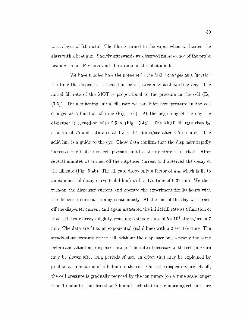
80
was a layer of Rb metal. The �lm returned to the vapor when we heated the
glass with a heat gun. Shortly afterwards we observed uorescence of the probe
beam with an IR viewer and absorption on the photodiode.
We have studied how the pressure in the MOT changes as a function
the time the dispenser is turned-on or o�, over a typical working day. The
initial �ll rate of the MOT is proportional to the pressure in the cell (Eq.
(1.5)). By monitoring initial �ll rate we can infer how pressure in the cell
changes as a function of time (Fig. 5.4). At the beginning of the day the
dispenser is turned-on with 2.5 A (Fig. 5.4a). The MOT �ll rate rises by
a factor of 75 and saturates at 1:5 � 109 atoms/sec after 4-5 minutes. The
solid line is a guide to the eye. These data con�rm that the dispenser rapidly
increases the Collection cell pressure until a steady state is reached. After
several minutes we turned o� the dispenser current and observed the decay of
the �ll rate (Fig. 5.4b). The �ll rate drops only a factor of 4.4, which is �t to
an exponential decay curve (solid line) with a 1=e time of 0.37 min. We then
turn-on the dispenser current and operate the experiment for 10 hours with
the dispenser current running continuously. At the end of the day we turned
o� the dispenser current and again measured the initial �ll rate as a function of
time. The rate decays slightly, reaching a steady state of 5�108 atoms/sec in 7
min. The data are �t to an exponential (solid line) with a 2 sec 1=e time. The
steady-state pressure of the cell, without the dispenser on, is nearly the same
before and after long dispenser usage. The rate of decrease of the cell pressure
may be slower after long periods of use, an e�ect that may be explained by
gradual accumulation of rubidium in the cell. Once the dispensers are left o�,
the cell pressure is gradually reduced by the ion pump (on a time scale longer
than 10 minutes, but less than 8 hours) such that in the morning cell pressure

81
is very low.
We have observed no deterioration in Rb vapor pressure, as inferred
by MOT �ll time, for the single dispenser we have used since construction of
the apparatus. We therefore infer that the dispenser lifetime is at least 2 years
when run approximately 10�12 hrs/day at 2:2�2:6 A. We note that this is the
estimated lifetime in a glass cell environment. In our experience, Rb dispensers
exhibit shortened lifetimes in steel-(rather than glass-)based vacuum chambers.
The steel apparently consumes the Rb and the dispenser lifetime depends on
the amount of steel surface area and the con�guration of the dispensers relative
to the surfaces.
5.2 Collection MOT
5.2.1 MOPA Trap Laser
We achieve rapid �lling of large atom numbers in the Collection MOT
through large beam size but also high total power. The large power exceeds
the output of even the most powerful diode lasers, and typically implies the use
of a Ti:Sapphire laser to reach the desired 0:5�1 Watt. We instead introduced
a substantial simpli�cation for generating high-power infra-red light by using
a solid-state Master Oscillator Power Ampli�er (MOPA) system. The Master
Oscillator (MO) is a low-power diode. Some of the light from the diode passes
through a Power Ampli�er (PA) chip, which is basically a semiconductor gain
medium, that ampli�es the power by nearly a factor of 100 and gives almost
0:5 Watts of total output power.
The layout for the system is shown in Figure 5.5. The master diode
laser beam �rst passes through an optical isolator and a lens then focuses it

82
0 1 2 3 4048
1216
(a)
0 1 2 3048
1216
τ = 0.37(1) min(b)
0 1 2 3 4 5 6 7468
1012
τ = 2(1) min
Initi
al C
olle
ctio
n M
OT
Fill
Rat
es (
108 /s
ec)
(c)
Time (min)
Figure 5.4: Change in the Collection MOT initial �ll rate as a function of time
the dispenser is on or o�. (a) Rise in �ll rate when dispenser is turned-on at
2.5 A at the beginning of the day. Five minutes after initially turning on the
dispenser, the �ll rate saturates. The solid line is a guide to the eye. (b) We
then measure the decrease in the rate after the dispenser is turned o�. (c)
Decrease in the Collection MOT �ll rate when the dispenser current is turned-
o�, after 10 hrs of continuous dispenser operation. The solid lines in (b) and
(c) are exponential �ts to the data with 1=e times given in the �gures.
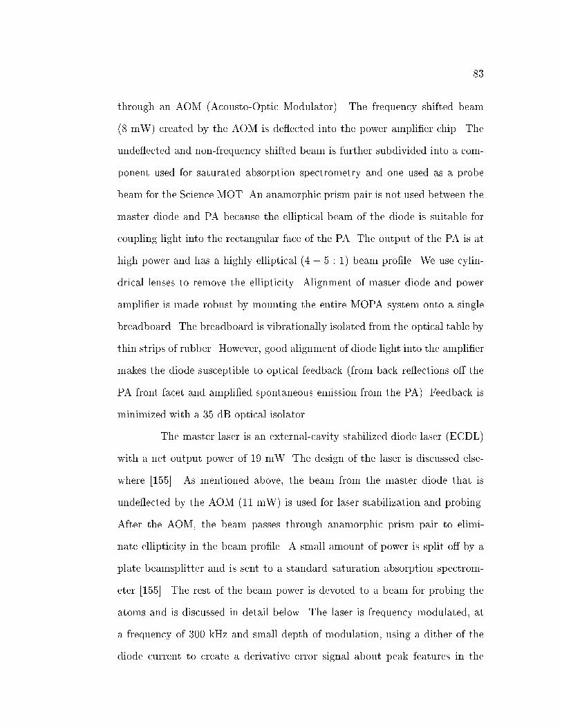
83
through an AOM (Acousto-Optic Modulator). The frequency shifted beam
(8 mW) created by the AOM is de ected into the power ampli�er chip. The
unde ected and non-frequency shifted beam is further subdivided into a com-
ponent used for saturated absorption spectrometry and one used as a probe
beam for the Science MOT. An anamorphic prism pair is not used between the
master diode and PA because the elliptical beam of the diode is suitable for
coupling light into the rectangular face of the PA. The output of the PA is at
high power and has a highly elliptical (4 � 5 : 1) beam pro�le. We use cylin-
drical lenses to remove the ellipticity. Alignment of master diode and power
ampli�er is made robust by mounting the entire MOPA system onto a single
breadboard. The breadboard is vibrationally isolated from the optical table by
thin strips of rubber. However, good alignment of diode light into the ampli�er
makes the diode susceptible to optical feedback (from back re ections o� the
PA front facet and ampli�ed spontaneous emission from the PA). Feedback is
minimized with a 35 dB optical isolator.
The master laser is an external-cavity stabilized diode laser (ECDL)
with a net output power of 19 mW. The design of the laser is discussed else-
where [155]. As mentioned above, the beam from the master diode that is
unde ected by the AOM (11 mW) is used for laser stabilization and probing.
After the AOM, the beam passes through anamorphic prism pair to elimi-
nate ellipticity in the beam pro�le. A small amount of power is split o� by a
plate beamsplitter and is sent to a standard saturation absorption spectrom-
eter [155]. The rest of the beam power is devoted to a beam for probing the
atoms and is discussed in detail below. The laser is frequency modulated, at
a frequency of 300 kHz and small depth of modulation, using a dither of the
diode current to create a derivative error signal about peak features in the

84
Diode
Laser
(MO)
Power
Amplifier
(PA)
Shutter
Optical
Isolator AOM
To
Saturated
Absorption
&
Probe
To Beam Shaping
Optics
Breadboard
L1 L2
M2
M1
M3
Figure 5.5: Layout of the MOPA laser system used for trap light in the Col-
lection MOT and probe light cold atoms in the Science MOT. M = mirror; L
= lens

85
saturated absorption spectrum. We stabilize the laser frequency by using the
slope of the dispersion curve to servo the MO laser PZT and diode current
about the desired absorption peak. Since we use the MOPA for MOT trapping
and near-resonant probing we peak-lock to the cross-over transition between
the 5S1=2F = 2 ! 5P3=2F0 = 2 and 5S1=2F = 2 ! 5P3=2F
0 = 3 transitions
that lies 133:5 MHz to the red of the \cycling" F = 2 ! F 0 = 3 transition.
The MOT detuning is set by choosing the frequency shift of the de ected beam
(� 120 MHz).
5.2.2 Repump Light
Our system requires much less power on the 5S1=2F = 1! 5P3=2F0 =
2 repumping transition. We generate enough repump light for both Collection
and Science MOTs from a single ECDL with total output of 17 mW. We divide
the beams with a �=2 plate and polarizing beam splitter cube and send 2 mW
to the Collection MOT. As described above, the frequency of the repump laser
is also stabilized to the F = 1 ! F 0 = 2 saturated absorption peak using a
300 kHz current dither. We found that both MOTs operate well at zero de-
tuning so that a direct peak-lock is su�cient. After the saturated absorption
spectrometer, an optical isolator prevents feedback to the diode. Lastly, the
diode laser and spectrometer is enclosed in a black-cardboard housing to con-
tain scattered photons. We have found this eliminates optical depumping of
F = 1; mF = �1 state during evaporative cooling.
5.2.3 MOT Con�guration
To take full advantage of the 38 mm window diameter we use 50
mm optics throughout the MOT set-up. We combine the MOPA and repump

86
light, and then use two telescopes and one polarizing beam splitter plate to
produce three beams that are roughly rectangular-shaped with approximate
1=e dimensions of 25 � 20 mm. The irregular shape and pro�le is the result
of (non-optimal) beam shaping optics and AOMs. The imperfections in the
beam do not prevent us from rapidly accumulating large numbers of atoms
in the MOT. We use 50 mm mirrors and �=4 plates, which minimize beam
clipping and power loss, to direct the beams into the cell in a standard 3-
beam retro-re ected MOT con�guration. The quadrupole �eld for the MOT
is generated by a pair of air-cooled coils wound from magnet wire and placed
in anti-Helmholtz con�guration. Stray magnetic �elds, especially from the
nearby ion pump, are compensated by three, unpaired shim coils. We monitor
the MOT number with a PD and position of the MOT with a low-cost CCD
camera.
5.2.4 Alignment and Operation
Alignment of the Collection MOT is non-critical because the trap
beams are so large and low temperature in the MOT is not important for
transfer. The basic goal is to occupy as much of the clear aperture of the
windows as possible with MOT light. We balance the beam intensities and then
roughly retro-re ect the beams to achieve reasonable MOT �ll-rate and total
number. We optimize the rate and number by adjusting the retro-mirrors while
monitoring the PD signal. This procedure also places the atoms nearly along
the transfer tube axis. We then optimize the transfer by slight adjustments to
the currents in the shim coils; these adjustments do not degrade either MOT �ll
rate or total number. Typically we run the MOT at 10 G/cm, using a total of
� 300 mW in the trapping beams once they reach the Collection cell, running
87
the dispenser current at 2:3� 2:8 A for a background pressure of roughly 10�9
Torr. We achieve a maximum total �ll of 1:5� 109 atoms in the MOT with a
1=e �ll time of 1� 2 sec.
5.3 Science MOT
5.3.1 General Considerations
The purpose of the Science MOT is to provide an environment for
loading a purely magnetic trap, at the lowest temperatures and highest densi-
ties possible, in a low-background pressure. The su�cient conditions are: (i)
hold > 109 atoms; (ii) optically cool atoms to sub-Doppler temperatures in a
molasses; (iii) optically compress the atoms in a Compressed MOT (CMOT);
(iv) allow alignment of optical trap and magnetic trap for smooth transfer of
atoms; and (v) optical access to probe small atom clouds (10's of �m).
5.3.2 Lasers
The trapping light for the Science MOT is generated by a single ECDL
that is o�set peak-locked to the cross-over transition between the F = 2 !
F 0 = 2 and F = 2 ! F 0 = 3 transitions. The scheme is completely identical
to the lock used for the MOPA laser except that the de ected beam is sent to
the spectrometer and the unde ected beam is sent to the MOT. The reason
is that we did not want to a�ect the MOT alignment by changes to the AOM
frequency, which in turn also shift the beam position. The net beam power out
of the laser is 55 mW while the power after the optical isolators and AOM's,
but before division of the beam into the separate MOT beams, is 20 mW.
Repump light on the F = 1 ! F 0 = 2 transition is provided by

88
our single repump laser. The total power sent to the Science MOT is 2 mW.
Initially this laser was locked to the side of the saturated absorption feature
and proved more than adequate to make reproducible Bose condensates in the
F = 2; mF = 2 state. We switched to a peak-locked repump only after we began
to produce condensates in the F = 1; mF = 1 state, when we require frequency-
stable repump light for optically pumping the atoms during the probe pulse.
We also modify the delivery of the repump light to the Science MOT for the
CMOT stage. We divide the repump beam into a main beam of 6 mW and
a bypass beam of only 35 �W. The set-up for the repump bypass is shown in
Figure 5.6.
5.3.3 Quadrupole Coils
The quadrupole �eld for the Science MOT serves two ends. In the
MOT loading phase, it generates the modest �eld gradient (axially, B0
z = 17
G/cm) for the MOT. In the magnetic trap phase, the coils must safely generate
signi�cantly higher gradients, handling kW's of power and still possess a rapid
turn-o� time. The quadrupole coils are constructed with 18" hollow copper
tubing that is wound into two coils. Each coil is 3 turns tall by 4 turns deep
and forms an annulus with rectangular cross section of 1:5 cm tall by 1:75
cm deep (Figure 5.7). The inner diameter of the coil is 1:27 cm and the inner
surface separation of the coils is 3:5 cm. The windings are electrically insulated
from each other by sheathing the copper in heat-shrink tubing. The coils are
made structurally solid by potting them in epoxy. We water cool the coils with
a wall-pressure ow of room temperature water through the hollow copper
tubing.
The coils are connected in series, in a nearly anti-Helmholtz con�g-

89
Main
Shutter
Bypass
Beam
Bypass
Shutter
� /2
Plate
� /2
Plate
PBS 1 PBS 2
M 1 M 2
Main
Beam
To
Atoms
Figure 5.6: Bypass scheme for the repump light to the Science MOT. PBS =
Polarizing Beam Splitter Cube; M=mirror

90
uration. Since maximizing gradient is our primary goal, the coils are placed
as close to the atoms as possible, with a distance generally limited by optical
access. Each coil has a resistance of about 6:8 m. We supply the coils with
a 6 V, 300 A power supply. The supply voltage and lead resistances limit the
ultimate �eld gradients to be B0
z = 305 G/cm at around 260 A. At 6 V and
13:6 m the max current is 441 A and max power dissipation is 2700 Watts.
However, �nite resistance in wires and connectors limits the maximum voltage
drop across the coils to 3:5 V and power dissipation to 1600 W. From the coil
geometry we calculate the inductance L of the coils [156] is equal to 4:9 �H.
Treating a single coil as an inductor in series with a resistance of R = 6:8
m gives the 1=e decay time of the current: � = L=R = 720 �sec. We mea-
sure 900 �sec. The currents (and hence �elds) are stabilized using a bank of
water-cooled power FET's as described in [157].
5.3.4 Shim Fields
Stray magnetic �elds inevitably shift the zero point of the magnetic
�eld from the center of the MOT beams, and alter the delicate overlap between
MOT and magnetic trap. We minimize stray �elds by assiduously avoiding
magnetic bases and magnetic metals (screws, mounts, vacuum components)
near the glass cell. Stray �elds are shimmed by three, unpaired coils. The
divergence of the shim �eld is so slight as to be insigni�cant to operation of
the MOT, molasses or magnetic trap. We also switch the currents through
the shim coils to di�erent values. One set of currents is optimized for loading
the MOT to maximum �ll from the Collection cell. The other set of currents
optimizes the molasses cooling and TOP loading, usually by observing the
isotropy of the molasses expansion, but sometimes also by optimizing number

91
3 turns
4
turns
3.5
1.5
1.75
1.27
Figure 5.7: Cross-section of the Quadrupole Coils. There are two coils, with
symmetry axis parallel to gravity (and the long edge of the page). Dimensions
are in cm.

92
in the condensate.
5.3.5 MOT Con�guration and Alignment
The Science MOT uses a con�guration of six independent beams. Al-
though the 6-beam approach is more cumbersome to align, previous experience
suggested that 3-beam Rb MOTs did not �ll to as large a number or perform
as robustly [152]. One factor is optical attenuation: With 109 atoms in a MOT
cloud of 0.5 cm diameter and trap light detuning of 3 linewidths the absorption
of a single pass through the cloud is 30%! Losses from scattering o� uncoated
optical surfaces (4%) can also shift the equilibrium position of the MOT away
from the zero-point in quadrupole magnetic �eld, due to imbalances in beam
intensity. Therefore MOT stability is reduced, as is the e�ciency of molasses
cooling.
Because alignment is more challenging, we emphasize ease of coupling
light into the cell, from all directions, with the least amount of loss. We use
two-inch optics wherever possible and especially far from the cell, where small
beam clipping means signi�cant loss of power. The larger optics also simplify
alignment because the MOT beams are much smaller in diameter than the
optics. Other notes on optics and design:
� Near the cell, large optics limit optical access so we more carefully align 25
mm dia PBS cubes and �=4 plates immediately before the cell.
� Use of Dielectric mirrors throughout the optical layout minimize loss of power
and preserve wavefront integrity. Nonetheless, the AOM's and optical isolator
degrade the wavefront quality substantially.
� Mounts are very minimal short posts and post-holders. Larger mounts limit
access to the cell without improving MOT stability.

93
We align the MOT with the following procedure. We balance the
power for each direction and optimize the throughput. We designate three
especially di�cult-to-align directions as the \Cardinal" directions, and align
those three beams to be centered and normally-incident on the cell windows.
Aperturing the beam sometimes helps, but it is most important that the ma-
jority of the irregular beam pro�le is centered on the window. This ensures
that most of the power reaches the atoms. Next, we align the three \anti-
Cardinal" beams to overlap with the \Cardinal beams". The overall procedure
usually produces a MOT of many 108 atoms with an irregular cloud shape.
The problem may be in the irregular pro�les of the MOT beams. In any event,
we optimize total number of atoms in the MOT by monitoring a PD signal and
adjusting the anti-Cardinal beam alignment only . This tends to produce MOT
clouds that are more round-shaped, and which contain large, stable numbers
of atoms (3�9�109 max). The molasses also performs best in this alignment.
5.3.6 MOT Operating Characteristics
Even with only 106 atoms, most MOTs operate in the constant den-
sity regime. Thus, adding more atoms necessarily means increasing the cloud
diameter. The ultimate limit to the total number of atoms contained in a
MOT is therefore the size of the MOT beams and the shape of the intensity
pro�le. Speci�cally, integrity of the beam pro�le and details of the beam qual-
ity at the edge of the beams, which comprise large trap volumes, can strongly
a�ect number in the MOT. With 109 atoms in our MOT, operating at a de-
tuning of 18 MHz, the cloud diameter is 5�7 mm (de�ned as the full-width at
half-maximum (FWHM)) and the mean density is approximately 1010 � 1011
atoms/cm3. Each beam has a total power that is typically 2 mW, with a

94
FWHM equal to roughly 1.5 cm (although the pro�les are fairly non-Gaussian)
giving an average intensity of 0:9 mW/cm2
We make several observations about our MOT, from which we connect
large sensitivity of max MOT �ll and low optical cooling temperatures to beam
alignment and spatial pro�le. We note that:
�Signi�cant re-alignment of the beams, even after the MOT beams seem
aligned and retrore ected, is necessary to reach the maximum MOT �ll. This
suggests that details of the beam pro�le, in addition to beam alignment, are
important.
�Small beam power imbalance can seriously degrade the total �ll, the molasses
temperatures, or both.
�An intermediate alignment of the beams can produce MOT clouds of 1�2�109
atoms that are highly unstable. The clouds have large, wispy arms and lose
many atoms at irregular intervals. Using this fairly large, unstable MOT we
can still produce BEC's, but with generally fewer atoms and less repeatability
than in our best MOT alignment.
�The best MOT numbers and temperatures are obtained when the cloud ap-
pears very regular and round. Number of atoms in the condensate is largest,
and most reproducible, under these conditions.
Lastly, I mention the issue of MOT lifetimes. The MOT lifetime is a
useful diagnostic for inferring the background pressure of the Science cell. The
time rate-of-change of the number of atoms in the MOT is well-understood
in terms of a loss rate due to background gas collisions, which is proportional
to number N , and a loss rate due to light-assisted collisions between atoms
in the MOT, which is proportional to density squared (see Eq. (1.6)). In
the low background pressures of the Science MOT, the MOT collection rate

95
is negligible and we observe no formation of a MOT directly from the vapor.
Hence, knowledge of the background pressure is determined from the loss of
atoms from the MOT. However, a simple analysis shows that light-assisted
collisions complicate the interpretation of the MOT lifetime in terms of the
background vapor pressure. For a Rb MOT whose trap beams are red-detuned
several linewidths from resonance, and which has total beam intensity equal
to several times the saturation intensity, the light-assisted decay rate con-
stant is � � 10�12 cm3/sec [158]. A MOT with rather modest density of 1010
atoms/cm3 will therefore have a light-limited lifetime of 100 s. With approxi-
mately 108 atoms in a MOT whose trap beams are red-detuned 20 MHz, and
which have a total intensity of 10 mW/cm2, we measure lifetimes of about 150
sec. We expect that our background collision rate is much smaller than that.
We suppressed light-assisted losses by reducing the number of atoms, which
decreases the MOT density. Using only 2� 106 atoms, we measure MOT life-
times of 450 � 500 sec. Reducing the total MOT intensity also increases the
observed MOT lifetime. The longest observed lifetimes are consistent with a
background pressure below 10�11 Torr.
5.4 Collection MOT to Science MOT Transfer
5.4.1 General Scheme
Atoms are transferred from the Collection cell to the Science cell by
applying a near-resonant laser beam that pushes atoms down the transfer tube
separating the Science cell from the Collection cell. The transfer e�ciency
is bolstered by using a hexapole magnetic �eld along the transfer tube that
provides radial magnetic con�nement. Several strategies work in the transfer.

96
Typically we accumulate atoms in the Collection MOT, turn o� the MOT,
apply a short pulse of the push laser, and then recapture the atoms in the
continuously operating Science MOT. We repeat the process until the Science
MOT reaches the desired number of atoms. We have also successfully trans-
ferred atoms using a continuous push beam and a Collection MOT cloud (the
cloud is slightly o�set from the axis of the transfer tube and push beam). This
creates a sort of Low-Velocity Intense Source [159] loading, whereby atoms are
continuously pushed out of the MOT and travel down the tube. Although we
have not compared the two approaches in detail, we have observed the pulsed
mode tends to have better transfer e�ciency and requires less time to �ll the
Science MOT. In the following sections I describe our standard procedure for
transferring in the pulsed mode.
5.4.2 Hexapole Magnets
The transfer e�ciency is boosted considerably by a hexapole magnetic
�eld along the transfer tube. The magnetic potential is harmonic in the radial
direction of the tube and prevents atoms, with slight radial velocities, from
colliding with the walls and hence being lost during transfer. The hexapole
�eld is created by six strips of permanent magnets which form a hexagonal ar-
rangement around the tube. To provide maximum con�nement, the magnets
rest directly on the tube and are conveniently held together around the tube
by their self-attraction. Small breaks in the magnet strips, due to con at joints
or transverse tubes for the ion pumps/magent valve, do not cause enough tran-
verse displacement on the atoms during their ight down the tube to degrade
e�ciency.

97
5.4.3 Push Beam
The push beam is 6:5 mW derived from the main MOPA beam used
for the Collection MOT. The beam is directed down the transfer tube, through
the access window of the Collection cell, and is brought to a shallow focus
near the Science MOT. Just before the transfer window, the beam is circularly
polarized with a �=4 plate. No magnetic �eld is used to create a quantization
axis during the optical push. The push pulse duration is controlled with a
mechanical shutter whose minimum cycle time to turn on and o� is about
1� 2 ms.
5.4.4 First-Time Alignment
The best approach to observe transfer is to build both MOTs, as-
signing the polarizations and quadrupole �eld directions of the Science MOT
based on a working Collection MOT. The transfer signal is then an unam-
biguous cloud that is observed with a CCD camera. Even small numbers of
transferred atoms are well-detected by simply repeating the push cycle and
watching the Science MOT cloud accumulate. Without building the Science
MOT, we monitored the atoms that reach the Science cell, causing them to
uoresce with a probe beam transverse to their velocities, and detecting the
uorescence with a PD. This method gives information about the velocity dis-
tribution and group velocity of the atoms, but tends to undercount the total
number transferred. Generally, use as many atoms and as much push power
as possible during �rst alignment. The beam direction and Collection MOT
position are easily chosen by sending the push beam through both transfer
windows and adjusting the shim coils of the Collection MOT until you see the

98
cloud, in the Collection MOT, become distorted by the push light. The ini-
tial detunings and intensity are set by maximizing the distortion of the MOT
cloud.
5.4.5 Transfer Procedure
We transfer atoms by applying the push beam to the Collection MOT
and turning o� the MOT trap light. The atoms are accelerated up to 20 m/sec
(and out of resonance with the push beam) in under 1 msec and reach the
Science MOT in approximately 20 msec. The push light remains on during
the entire ight of the atoms, after which (at 30 msec) the push turns o�, and
the trap light and �eld gradient of the Collection MOT turn-on again. The
hyper�ne repump light remains on during the entire cycle, initially so that
atoms scatter su�cient photons to be pushed down the tube, and later out of
convenience. The Collection MOT then rebuilds for 750 msec in preparation
for another transfer. The details of the timing are given in Figure 5.8.
We monitor the progress of the �ll of the Science MOT by triggering
a storage scope to record the MOT uorescence every fourth transfer. The
uorescence, collected on a PD, is proportional to the number of atoms in the
Science MOT. Our computer checks the uorescence to determine when the
MOT has �lled to the desired number of atoms, and hence when to terminate
loading. When the number in the Science MOT is within about 2�108 atoms of
the total �ll, the computer switches to a an abbreviated rebuild time, between
transfers, of only 250 ms. The timing of events is suitably compressed to
detect uorescence at the time given in the bottom panel of Figure 5.8. The
shorter build time allows a gradual approach to the desired �ll and reduces the
variation in the �nal number loaded into the Science MOT.

99
0 10 20 30 40 50 60 70 80 90 200 225 250
Don't Measure
MeasureFluorescence
Detection timing only every 4thshot, or when science MOT within
108 atoms of desired total.
FluorescenceDetect
Time (ms)
0 10 20 30 40 50 60 70 80 90 700 725 750
0
5
10
15Axial
Gradient(G/cm)
MOT Trap Light
ShutterLight Off
Light On
Light Off
Light On
PushShutter
MOT Detuning
Push Detuning
Push AOMTrigger
Figure 5.8: Timing of the Collection MOT to Science MOT Transfer. (a)
Pulse AOM brie y shifts MOPA frequency to push detuning. (b) Status of
push shutter. (c) Collection MOT trap light shutter. (d) Collection MOT
axial quadrupole magnetic �eld gradient. (e) Trigger to record uorescence
signal on photodiode for monitoring progress of Science MOT �ll.

100
5.4.6 Final Notes on Transfer
We estimate the transfer e�ciency is about 25%. We tend to un-
dercount the Collection MOT number because the Collection MOT is larger
than the �eld-of-view of our imaging PD. Optimal transfer of atoms generally
is achieved by adjusting the power, detuning polarization and alignment of the
push beam, as well as the position of the Collection MOT. The beam occupies
most of the input window to the Collection cell. When the beam is passed too
close to the Science MOT it is clearly visible because each transfer produces
a transient displacement of the Science MOT cloud, which limits the transfer
e�ciency for large MOT clouds.
The magnetic valve is left open during the entire transfer cycle, and
throughout the day while the experiment is active. When the experiment is
not in use, we slide the magnet plug across the transfer tube to minimize
the integrated ux of Rb down the tube. In principle, we can open/close the
valve each shot, or every experimental cycle, but we have never observed a
degradation of the Science MOT pressure leaving the tube open even for 24
hours.
5.5 TOP Magnetic Trap
The TOP trap is made of six coils. The spherical quadrupole magnetic
�eld is generated by the quadrupole coil (Section 5.3.3) whose symmetry axis
is parallel to the direction of gravity. The rotating bias �eld is created by two
pairs of coils, each of which creates a uniform magnetic �eld in the center of the
cell, driven 90� out-of-phase. Each coil is actually shaped as an ellipse in order
to wrap them directly to the glass cell (as explained below). The coil diameters

101
are 3 cm (horizontal) and 1.5 cm (vertical), and the coils are placed 1.7 cm
from the center of the trap. The �eld shimming coils, described in Section
5.3.4, cancel stray magnetic �elds and align the MOT with the magnetic trap.
The theory of the TOP trap is given in Chapter 6 and Appen. C.
The TOP coils are also water cooled using a substantially di�erent
design than the quadrupole coils. We require less cooling capacity but more
winding exibility for the TOP coils compared to the quadrupole coils. Some
cooling is necessary because we dissipate up to 180 Watts through the coils. As
a second requirement we also wanted to wrap the coils very close to the cell to
maximize the TOP bias �eld per amp-turn, requiring much more freedom and
exibility in the coil winding than allowed by hollow copper tubing. The recipe
for the TOP coils is as follows. We insert three sections of 22 AWG magnet
wire into a poly o tube of 18" outer diameter. The wire sections are electrically
connected in series. The poly o is wound directly onto the experimental glass
cell to form a pair of approximately Helmholtz separated coils with three (nine)
poly o (magnet wire) windings in each coil. A second poly o/magnet wire tube
is prepared and similarly wrapped, though 90� o�set from the �rst coil pair,
around the glass cell. Room temperature water is pushed through the poly o
at wall pressure to cool the wires. The net ow is extremely small, but is
su�cient to handle the maximum power when generating rotating bias �elds
of up to 50 G.
The TOP coils are driven from a high-�delity sine wave that is am-
pli�ed through a voltage-controlled gain. The sine wave is divided into two
channels which have separately adjustable gain and adjustable relative phase.
The channels are separately ampli�ed by a two-channel audio ampli�er. The
maximum output power of the audio amp is 180 W and must be impedance
102
matched to the TOP coils. We use a pair of home-built transformers wound
around magnetic ferrite cores to both impedance match and step down (up)
the voltage (current). Small di�erences in coil size and relative phase-shifts
require a careful calibration of the actual TOP �eld. We detect the rotating
�eld with two identical 25 turn, 2.5 cm dia pick-up coils whose axes coincide
with the TOP coil pairs. The detection coils are placed at the same distance
from the atoms as the TOP coils. The induced EMF is integrated and output
to a scope to create a Lissajou �gure whose amplitude and phase are propor-
tional to the rotating magnetic bias �eld. Monitoring the Lissajou, and using
our gain and phase adjustments, we can create a nearly circular (within 5%)
or a highly elliptical rotating �eld. The rotating �eld is a natural quantization
axis for the experiment. We utilize the �eld by synchronizing critical probing
and optical pumping timing to the TOP rotation and computer triggers. The
synchronization is achieved with a home-built triggerable pulse-generator or a
commercially-produced pulse sequencer.
5.6 MOT-to-TOP Transfer
5.6.1 General Considerations
The protocol for transferring atoms from the Science MOT to the
TOP magnetic trap consists of:
MOT ! CMOT ! optical molasses ! optical pumping ! TOP
The MOT collects and holds the atoms until the desired initial number is
reached. The CMOT compresses the atoms into a smaller, more uniform
cloud and initiates the ramp-down of magnetic �eld for molasses. The optical

103
molasses precools the atoms to sub-Doppler temperatures. Pulses of optical
pumping light transfer most of the atoms into the desired state for magnetic
trapping. Finally, the TOP is turned on by quickly turning-on the rotating
bias and increasing the quadrupole gradient.
5.6.2 Prelude to Transfer
After the �nal load of atoms arrives from the Collection MOT, but
before initiating the following procedure to load the TOP trap from the MOT,
we wait 250 msec. The lifetime of the MOT is longer than 100 sec so little
of the gas sample is lost during the short wait. The wait permits the MOT
to thoroughly settle after the last injection of atoms. The wait time is also
useful for technical housekeeping such as setting program ags and initiating
equipment for later use.
5.6.3 CMOT
The CMOT is one of the least well-characterized stages of the exper-
iment. The previous comprehensive study of the CMOT [19] operated with
only � 107 atoms, using di�erent detunings, trap light intensities and �eld
gradients. The CMOT we use is optimized to transfer the most atoms, at low
temperature, into the TOP trap and little careful study has been done. The
CMOT stage lasts 30 ms. First, the detuning of the trap laser is shifted to 32
MHz red of the cycling transition (Fig. 5.9a). Immediately (1 ms) later, we
dramatically reduce the repump light intensity by allowing only the repump
bypass to illuminate the atoms (Fig. 5.11a). Next, we ramp down the axial
quadrupole gradient from 17:4 to 5:2 G/cm in ten, 1 msec steps. We leave the
atoms in this reduced gradient for 10 ms, and �nally ramp the gradient o� in

104
ten, 1 ms steps. See Fig. 5.10a. The trap laser is then red-detuned 45 MHz
from resonance to begin the molasses stage (Fig. 5.9a). During the second 10
ms period, we change the currents in the Science MOT shim coils from their
values optimized for MOT loading to values optimized for the TOP loading
(Fig. 5.10c). Recently, we have also found that not increasing the trap laser
detuning during the CMOT enhances the �nal number in the condensate, de-
spite little change in the observed e�ciency of transferring atoms into the TOP.
We speculate that the bene�cial e�ects of (i) reduced repump light intensity,
(ii) reduced �eld gradient, and (iii) reduced detuning may be understood qual-
itatively in terms of increasing the region of the trap over which the Stark shift
is large compared to the Zeeman shift of the atoms. In this region, the cloud
that experiences strong polarization gradient (sub-Doppler) optical forces, as
opposed to the weaker, spontaneous scattering (Doppler) optical forces which
a�ect the rest of the cloud. All three e�ects in the CMOT therefore improve
the initial conditions for evaporation by cooling and/or compressing the cloud.
5.6.4 Molasses Cooling
The molasses lasts 10 msec. During the molasses, the quadrupole
�eld gradient remains o� (Fig. 5.10a) and the only repump light is supplied
by the bypass beam (Fig. 5.11, a and b). Because of technical problems we
are unable to re-lock the laser at the molasses detuning (Fig. 5.9c), but over
the brief duration of the stage we observe very little drift in frequency.
5.6.5 Optical Pumping
Next, we perform optical pumping on the atomic sample to transfer
most of the atoms into the F = 2; mF = 2 or F = 1; mF = �1 or both states.
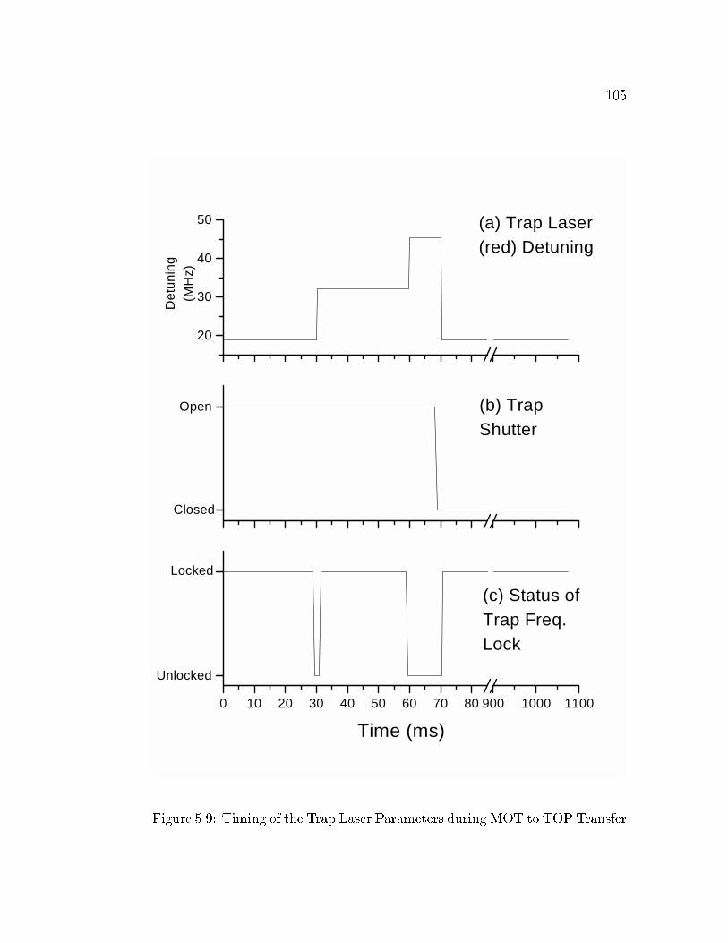
105
0 10 20 30 40 50 60 70 80 900 1000 1100
Unlocked
5
(c) Status ofTrap Freq.Lock
Locked
Time (ms)
0
Open (b) TrapShutter
Closed
20
30
40
50 (a) Trap Laser(red) Detuning
Det
unin
g(M
Hz)
Figure 5.9: Timing of the Trap Laser Parameters during MOT to TOP Transfer

106
0 10 20 30 40 50 60 70 80 900 1000 1100
0
10
20
150
200
250(c) Axial Quadrupole Gradient
Gra
dien
t(G
/cm
)
Time (ms)
0
20
40(b) TOP Bias Field
Fie
ld(G
)
0
TOP (a) ShimSettings
MOT
Figure 5.10: Timing of the magnetic �elds during MOT to TOP Transfer. (a)
Values for the shim coils, optimized either for Science MOT loading or TOP
magnetic trapping. (b) Amplitude of the TOP rotating bias �eld. (c) Axial
Quadrupole gradient.

107
0 20 40 60 80 100 900 1000 1100
0
Pulses On (d) OpticalPumping PulseTrigger
Pulses Off
Time (ms)
0
Open (c) OpticalPumping Shutter
Closed
Closed
0
Open(b) BypassRepump Shutter
0
Open
(a) Main RepumpShutter
Closed
Figure 5.11: Timing of the Repump and Optical Pumping during MOT to TOP
Transfer. Frame (a) shows the status of the shutter for the main repumping
light; when the shutter is open, light illuminates the atoms. Frame (b) is the
shutter for the bypass repumping light. Again, when the shutter is open, bypass
repump light illuminates the atoms. (c) Status of Optical Pumping Shutter.
(d) Optical Pumping Pulse Trigger. Optical pumping light illuminates atoms
in multiple pulses, but only for the time when the trigger pulse is high.

108
Because we use the TOP rotating bias �eld as a quantization axis (5.9 G, see
Fig. 5.10b), synchronization of optical pulses with the �eld is critical. We
initiate a pulse generator that triggers AOM's at speci�c delay times with a
certain phase relative to the TOP rotation. The duration of the AOM pulse is
also adjustable. We use the following di�erent pulse sequences to reach the:
� F = 1 state: Turn o� the F = 2 ! F = 3 MOT light 1 ms before turning
o� the F = 1 ! F = 2 bypass repump light (�gs. 5.9b and 5.11b, resp.),
followed by 72 pulses (each 400 �s long, 550 �s apart when the TOP trap
rotation frequency is 1800 Hz) from a 1 mW beam blue-detuned 9 MHz from
the F = 2! F = 2 and �� polarized. The 2-2 light depumps the F = 2 state
preferentially into the F = 1; mF = �1 state.
� F = 2 state: Keep repump light on while the F = 2 ! F = 3 light is
turned-o� and apply approximately 10 pulses (each 125 �s long) of 2-2 light
with �+ polarization to populate the F = 2; mF = 2 state.
� F = 1 and F = 2 states: Modify the F = 1 sequence, reducing the time-
delay between turn-o� of the F = 2! F = 3 and the F = 1! F = 2 bypass
repump light to less than 1 msec and reduce the number of 2 � 2 pulses to
achieve the desired relative mixture of states.
The fractional e�ciency of transferring the initial atom sample into
the TOP trap, in either the F = 1 or the F = 2 atomic state, is about 40-45%.
This number is a lower estimate to the optical pumping e�ciency since other
factors associated with the TOP trap limit the transfer (see below).
5.6.6 TOP Trap
Finally, we turn-on the TOP magnetic trap. There are several im-
portant considerations for selecting the initial trap parameters. First, we must

109
match the frequency of the TOP to the characteristic frequency for the atom
cloud de�ned by the spatial size and velocity spread of the atoms. Otherwise,
breathing modes are excited in the cloud that can be transformed into heat, via
anharmonic mixing. Second, the TOP trap must be su�ciently deep to contain
most of the molasses-cooled atoms. The depth of the TOP trap is 12
�kBBTOP ,
where � is the magnetic moment of the trapped state, and so a large trap
depth requires a large bias �eld. Third, the quadrupole gradient must be small
enough that the radius of the orbiting quadrupole zero (BTOP=B0
z=2) is much
larger than the atom cloud, which prevents spin- ip losses induced by the �eld
zero. We begin the TOP trap, for F = 1 atoms, with an axial �eld gradient
of 157 G/cm and a rotating bias �eld of 50 G (Fig. 5.10, a and b) to create a
trap depth of 840 �K, orbital radius of quadrupole zero of 3200 �m and trap
frequency of 20 Hz axially (7 Hz radially). We then adiabatically ramp the
gradient to 226 G/cm over 1 sec (Fig. 5.10a), increasing the trap frequency
to 29 Hz (10 Hz), to slightly increase the elastic collision rate as a prelude to
evaporative cooling. At the end of the transfer, we observe 40 � 45% of the
original 1� 2� 109 MOT atoms are loaded into the TOP trap.
5.7 RF Evaporative Cooling
5.7.1 Forced Evaporative Cooling through Induced RF Tran-
sitions
The TOP and Io�e-Pritchard magnetic traps con�ne atoms in the
low-�eld seeking states near the minimum in the magnetic potential. How-
ever, most of the spin states of the atoms are either untrapped or antitrapped
by the �eld minimum (see Fig.1.1 and discussion in Section 1.1.5). These

110
non-trapped states provide a natural mechanism for releasing atoms from the
magnetic trap by driving Zeeman transitions from the trapped and into the
non-trapped states. For the typical magnetic �elds involved (up to 50 � 100
G) we can use RF radiation techniques, as opposed to microwave or optical
methods that are more di�cult to implement. Evaporation is performed by
tuning the RF to induce transitions in atoms in the largest magnetic �elds,
which corresponds to the highest energy trapped atoms, and allowing the re-
maining sample to rethermalize to lower temperature. By ramping the RF to
lower frequencies we remove more energy from the sample so that it rether-
malizes to lower temperature. The general principles of evaporative cooling for
atomic systems were �rst discussed by H. Hess in 1986 [53]. The process of RF
evaporation was proposed by D. Pritchard [115].
5.7.2 Coupling rf to the atoms
In our experiment, the rf magnetic �eld is applied to the atoms with
an ampli�ed rf drive to one of the anti-Helmholtz coils of the quadrupole �eld.
This generates a magnetic �eld that oscillates parallel to the coil symmetry axis
and orthogonal to the quantization axis of the atoms (de�ned by the rotating
bias �eld). The rf �eld can therefore drive transitions between the trapped and
untrapped Zeeman sublevels.
The entire coupling circuit is shown in Figure 5.12. The RF is gener-
ated by a 0� 100 MHz GPIB controlled frequency synthesizer. The amplitude
is adjusted with a voltage controlled attenuator, and then the signal is am-
pli�ed by a constant 30 dB RF ampli�er. The output is connected to the
anti-Helmholtz coil through a pair of 0:68 �F capacitors. For a typical fre-
quency of 5 MHz, the coil inductance has an impedance of 150 , compared to

111
Amplifier
(+30 dB)
50 �
0.68 F
0.68 F
AH
Coil
4.9 H
50 �
Signal
Generator
Figure 5.12: Circuit for coupling an rf magnetic �eld to the atoms for forced
evaporative cooling

112
only 50 m for the capacitors. At higher frequencies the impedance continues
to be dominated by the coil inductance. At the low frequency end, we rarely
go below 4 MHz during evaporation. Thus, the e�ective load is always seen as
purely inductive.
5.7.3 Control of RF frequency and amplitude
One encounters several typical problems in this RF coupling scheme.
First, the impedance decreases during the RF ramp-down. We compensate for
the increased power delivered to the atoms by increasing the attenuation as
the frequency is lowered. Second, RF frequency generators have a �nite time
response to commands for changing their output frequency, which is typically
10 � 50 msec. We exercise care to allow the generator frequency to stabilize
during the ramp. Last, due to di�erent internal circuits that cover di�erent
frequency ranges, frequency generators sometimes exhibit unusual frequency
jumps as the frequency changes. We found the best solution is to use another
synthesizer.
5.7.4 Initial Conditions for Evaporation and Limitations to
E�ciency
The key to making runaway evaporative cooling is having a ratio of
the cloud's rethermalization rate to loss rate that is at least 100 � 200. The
rethermalization rate is simply the elastic collision rate divided by a factor of �
2:8 (as determined by Monte Carlo simulations [157]). In the UHV environment
of the Science cell the loss rate due to background gas is typically 0:002 sec�1.
Another loss process is the scattering of stray photons by magnetically trapped
atoms. Scattering can heat the atoms out of the trap and cause spin- ips into

113
untrapped states. We found that this can be a serious limitation to magnetic
trap lifetimes. We darken the Science cell, during the magnetic trapping phase
of the experiment, using the following measures:
� Multiple layers of cardboard light ba�es between lasers and apparatus
�Black plastic enclosure around the Science cell
�Cardboard enclosures around most mechanical shutters
�Isolate the repump laser in a separate cardboard enclosure to suppress unin-
tended optical pumping of atoms from the F = 1 state into the F = 2.
The other inelastic loss important to 87Rb is due to three-body recom-
bination. The rate constant is 3:5�10�30 cm6/sec, suggesting a recombination
lifetime in the initial stages of evaporation (when the density is perhaps only
1012 atoms/cm3) of 8 hrs! However, because the 3-body rate scales as the square
of the density this inelastic rate becomes important at densities approaching
those typical of a BEC of 106 atoms (1014/cm3)
When the trap losses are limited only by background collisions, the
minimum rethermalization rate necessary for runaway evaporation is about 0:3
sec�1, or an elastic rate of 0:7 sec�1. Fortunately in 87Rb, the elastic collision
cross-section is temperature-independent for the temperature range obtained
via optical cooling. Thus, we can enhance the collision rate by adiabatically
compressing the atoms because the elastic collision rate will scale as the square
of the trap frequency.
5.7.5 Evaporation Protocol
Once the minimum conditions on collision rate are met, evaporative
cooling works repeatably and is relatively insensitive to the exact details of
the pro�le of RF frequency sweep and magnetic trap compression. We ini-

114
tially ramp up the quadrupole gradient and then use several exponential ramp
sections to ramp down the RF frequency and TOP bias �eld. Exponential
ramping the RF cut value, in which the ramp rate is time-independent, has
the feature that, as the RF is swept down, the change in cut energy is always
a constant fraction of the total energy per unit time. For each ramp stage
we adjust the ramp rate and power of the RF. We increase the attenuation
of the RF as the frequency is ramped down to compensate for the decreasing
impedance of the RF coil. We are not overly generous in the amount of RF
power. Using more RF power than necessary to drive the RF transitions has
the e�ect of power broadening the transition probability, which reduces the en-
ergy selectivity of the RF knife and the evaporation e�ciency. The RF ramp
can proceed only as fast as the cloud rethermalizes and cools. Ramping faster
unnecessarily removes atoms that would rethermalize, also reducing e�ciency.
In the computer program which runs the experiment, the workhorse
procedure for our evaporation is a routine called coolexp. This routine ramps
the RF frequency and TOP bias �eld, simultaneously, or either one separately.
Coolexp is called with seven arguments: Coolexp Vi, Vf , fi, fc, ff , �, �. The
�rst two parameters Vi and Vf are the initial and �nal control voltages for the
ramp of the TOP bias �eld. fi and ff are the initial and �nal RF frequencies
of the ramp, while fc indicates the frequency corresponding to the center of the
trap. When fc = 0 Eqs. (5.1) show that the RF and bias �eld ramp together.
The pro�les look like:
fRF (t) = (fi � fc)exp((�r + �rt)t) + fc (5.1a)

115
BTOP (t) = BTOP (0)exp((�t + �tt)t) (5.1b)
�r = � (5.1c)
�r = � (5.1d)
�t = � ln
�Vf
Vi
�ln
�ff � fc
fi � fc
�(5.1e)
�t = � ln
�Vf
Vi
�ln
�ff � fc
fi � fc
�(5.1f)
Notice that the exponential ramp in coolexp actually employs a rate constant
that increases linearly with time: �i + �it. This allows additional exibility to
increase the ramp rate during a single Coolexp ramp.
In Tables 5.2 and 5.3 I present the speci�c evaporation steps we typ-
ically use for cooling atoms in the F = 1 and F = 2 states, respectively. The
di�erences in pro�les arise largely from two facts. First, atoms in the F = 2
state experience trap frequencies which are ap2 larger than for atoms in the
F = 1. Hence, collision rates are higher in the F = 2 for clouds of comparable
number. Secondly, loss rates for the two states di�er slightly, favoring slightly
di�erent ramp rates to obtain optimal e�ciency. Due to the long magnetic trap
lifetimes, we can begin evaporation at any time after the atoms are loaded into
the trap. We use this exibility to initialize various ags, long-time-constant
�lters and GPIB command sequences. Evaporation then follows the content

116
of Table 5.2 or 5.3. After the sequences are complete, the RF remains on for
400 msec at the �nal rf value which allows for passive evaporation and �nal
rethermalization of the cloud. The RF amplitude is then ramped o� via the
attenuator, and an RF switch with 60 dB attenuation interrupts the signal
path from the RF synthesizer to the ampli�er.
5.7.6 Evaporation Round-Up
Here are some typical numbers for initial conditions before evapora-
tion. For F = 1 atoms, we start with 1:5� 108 atoms at a temperature of 62
�K and a peak density of 9:3� 1010/cm3 in a fz = 45 Hz, fx = 16 Hz trap to
reach initial elastic collision rates of 3:7 sec�1. For atoms in the F=2 state, we
start with 1:7 � 108 atoms at a temperature of 91 �K and a peak density of
1:2�1011/cm3 in a fz = 65 Hz, fx = 23 Hz trap to reach initial elastic collision
rates of 5:7 sec�1.
Let me conclude by discussing the robustness of the evaporation to
speci�cs of the RF and spring constant ramp. If evaporation doesn't produce
reliably large BECs there is usually only one problem: Initial conditions have
deteriorated. A handful of problems that a�ect initial temperature and density
are:
� Poor molasses or CMOT due to (i) misalignment or intensity imbalances of
the MOT; or (ii) poor laser mode
� MOT and TOP not well-aligned and magnetic shims need adjustment
� Poor optical pumping
Second, a couple of problems degrade the magnetic trap lifetime:
� Insu�cient ba�ing of laser light
� Build-up of Rb in Science cell (The TSP must be run brie y to sublimate

117
Step No. Command
1 RF synth at 0:5 dBm output power
2 ramp rf attenuatora control voltage 0! 3 in 300 msec b
3 coolexp 0.85, 0.85, 80, 0, 67, -0.1, 0 c d
4 coolexp 0.85, 0.51, 70.2, 0, 42.1, -0.06, -0.001
5 coolexp 0.51, 0.1, 42.1, 0, 8.26, -0.04, -0.01
6 ramp rf attenuator control voltage 3! 2:68 in 80 msec
7 coolexp 0.1, 0.1, 8.26, 4.13, 6, -0.18, -0.02
8 ramp rf attenuator control voltage 2:68! 2:8 in 80 msec
9 coolexp 0.1, 0.1, 6, 4.13, 4.8, -0.5, -0.06
10 ramp rf attenuator control voltage 2:8! 2 in 80 msec
11 coolexp 0.1, 0.1, 4.8, 4.13, �nalrf, -0.17, -0.017
aMini Circuits ZAS 3bThe amplitude ramps reduce motion of the cloud in
the trap caused by RF transients that distort the magnetic
trap.cBTOP = 59VTOP where �eld is given in GaussdRF center frequency determined by the gF�B=hBTOP
where �B is the Bohr magneton and gF = 1=2 for 87Rb
Table 5.2: Evaporation steps for F = 1 atoms
Step No. Command
1 RF synth at �14 dBm output power
2 coolexp 0.85, 0.85, 80, 0, 67, -0.1, 0
3 coolexp 0.85, 0.58, 70.2, 0, 47.9, -0.001, -0.005
4 coolexp 0.58, 0.51, 47.9, 0, 42.1, -0.0075, -0.005
5 coolexp 0.51, 0.11, 42.1, 0, 9.08, -0.05, -0.005
6 coolexp 0.11, 0.11, 9.08, 4.54, 6, -0.15, -0.01
7 coolexp 0.11, 0.11, 6, 4.54, �nalrf, -0.1, -0.02
Table 5.3: Evaporation steps for F = 2 atoms

118
additional Titanium into the system and remove the excess Rb.)
5.8 Imaging System
5.8.1 Absorption
In the work described in this thesis, clouds of atoms are detected
by imaging the shadow of the atomic sample, caused by atomic absorption
of a near-resonance probe laser, onto a CCD camera. The F=2(1) atoms are
illuminated with a short pulse (10 � 30 �sec) of �+(-) polarized light with a
frequency tuned 0-20 MHz near the F = 2; m = +(�)2! F = 3; m = +(�)3
cycling transition. For the F = 1 atoms, a brief pulse of light tuned near the
F = 1 ! F = 2 transition optically pumps the atoms into the F = 2 state,
so that they can scatter many photons on the cycling transition. The optical
pulses are synchronized with the rotating bias �eld of the TOP which de�nes
a quantization axis for the atoms.
The atoms are viewed either in the magnetic trap or, more typically,
after a period of free-falling ballistic expansion lasting up to 20 ms. The ex-
pansion is often necessary because the FWHM spot resolution of the imaging
system is approximately 6 �m while the spatial extent of the condensate in the
trap is only 10 � 30 �m. Expansion also helps to diminish the high (several
100) on-resonant optical depths of condensates which saturate the absorption
image. In addition, high optical depth clouds behave like lenses for the probe
beam, greatly distorting the image of the shadow. We refer to this phenomena
as lensing. Depending on the choice of expansion time and frequency of trap
prior to release of the atoms, we reduce the optical depth, after expansion, by
a factor of about 10� 20. Similarly, adjusting the detuning of the probe light

119
from resonance e�ects a reduction of a factor of 10�30 in the observed optical
depth. Through judicious choice of detuning and expansion we usually observe
an optical depth of 1� 2.
5.8.2 Optics and CCD Camera
The probe light is taken from the unde ected beam of the Master
Oscillator (MO) laser after passing through an AOM. Recall that the AOM
is used for o�set-locking to the laser. We set the detuning of the probe beam
by shifting the probe frequency with another AOM, whose center frequency is
near 140 MHz, to counter the o�set-lock frequency of 133.5 MHz. The shifted
beam of the AOM is coupled into an optical �ber. The �ber spatially �lters
the probe beam and improves the beam-pointing stability. The beam has a
Gaussian transverse pro�le equal to 1.9 mm FWHM at the Science cell. We
typically operate at 230 �W of total power.
Figure 5.13 shows the imaging system for viewing cold atom samples.
Two lenses in a telescope con�guration (magni�cation 9.6) image the shadow of
the cloud onto the CCD camera. The �rst lens is a 2.5 cm dia, f = 6 cm placed
5.9 cm from the atoms. For the smallest samples light scattered from the cloud
is nearly at the focus of the �rst lens and is therefore nearly collimated as it
travels to the second lens. The second lens of 3.8 cm dia and f = 50 cm is
20.5 cm away from the �rst lens, and 50 cm in front of the CCD array to bring
the image into crisp focus. Both lenses are achromatic doublets to minimize
spherical aberrations. The speed of the imaging is determined by the aperature
of the window projected onto the �rst lens. That gives f=# = 6:0=1:7 = 3:6
and a di�raction limited FWHM spot size of 1:02� 0:78� 3:6 = 2:9 �m. The
larger diameter of the second lens captures all the light from the �rst and

120
prevents vignetting of the image. For viewing clouds much hotter than BEC
(typical of initial conditions in the magnetic trap) we add a de-magnifying
telescope to increase the �eld-of-view to properly capture the entirety of these
hot clouds.
We focus the imaging system on the atoms by viewing the tiniest
cloud of atoms, usually a small BEC. It is impractical to move the �rst lens
so we focus the system by moving the camera to �nd the image plane. We
use several criteria to de�ne \in-focus". First, we move the camera along the
optical axis until we observe the smallest clouds and the largest optical depth
with the probe tuned on-resonance. Because the lensing caused by the atoms
is at its worst when the probe is one-half linewidth detuned to either side of
resonance, we use small numbers of atoms viewed exactly on resonance. This
procedure usually yields a rather wide range of camera positions around the
minimum cloud size. We narrow-in on the image plane by exploiting the lensing
of the atoms. We detune to either side of resonance and recording the clouds'
optical depth, which changes with the camera position due to the lensing e�ect.
Moving the camera in a given direction through the image plane the optical
depth either increases or decreases depending on the sign of the detuning. The
intersection of the two curves of optical depth vs. position should occur at the
image plane. Focusing the system in this way we achieved minimum FWHM
spot sizes of 6 �m. These spots are clearly not di�raction limited. The large
minimum spot-size probably results from some residual spherical aberrations
in the optical system, but we have not worked to isolate the source or improve
upon the present resolution limit.
The shadow of the atom cloud is recorded on a triggerable Charge-
Coupled Device (CCD) camera. The camera output is digitized by a separate

121
CCD
Array
1.2 X 1.2
L1
f=6
2.5 dia
L2
f=50
3.8 dia
5.9
5020.5
Atom
Cloud
Figure 5.13: Schematic of the imaging system. Dimensions are in cm and the
drawing is not to scale.

122
electronic controller and the images are processed with numerical �tting rou-
tines. Camera, controller and software controls are commercially obtained
(Princeton Instruments), while the control software was written in-house. The
CCD is housed in a vacuum environment and cooled with a thermoelectric
cooler(unused). The CCD is a back-illuminated array, manufactured by SITe,
has 512� 512 pixels for an overall size of 12:3 � 12:3 mm. The pixels are 24
�m. The combination of back-illumination and a VIS/AR coating make the
quantum e�ciency 65% at 780 nm. The dynamic range of each pixel is 12 bits.
The controller operates in 12 bit (500 kHz) or 16 bit (150 kHz) modes. Finally,
the speci�ed readout noise is very low: 4-7 electrons at 50 kHz and 18-21 at 1
MHz.
5.8.3 Basic Imaging Procedure
In absorption, the observable is the optical depth (OD) of the atomic
sample at each point in space. For intensities of probe light, I0, that are small
compared to the saturation intensity, Is, the intensity I(~r) transmitted through
the cloud is given by Beer's Law:
I(~r) = Ioe�OD(~r) (5.2)
where OD(~r) =Rn(~r)�odz, n(~r) is the density distribution of the sample
and �o is the on-resonant optical cross-section at zero intensity. By detecting
the normalized transmission of the probe we deduce the spatial pro�le of the
cloud's OD:
123
OD(~r) = ln
�Io
I(~r)
�(5.3)
In practice, we measure optical depth by taking three images. First,
we image the atoms with the probe light (Shadow Frame). Second, we dump
the atoms from the trap and, approximately 1 sec later, record an image with
only the probe light present (Normalization or Light Frame). Finally, with no
light present at all, we record a Dark Frame that contains any electronic noise
or o�sets not due to light or atoms. In the �nal processing we calculate the
OD by subtracting the dark frame from both the light and shadow frames,
divide them and take their natural log on a point-by-point basis:
OD(~r) = ln
�Ilight � Idark
Ishadow � Idark
�(5.4)
If the probe light intensity is much more than 0:1Is the optical transi-
tion begins to saturate and the fractional absorption is no longer proportional
to the OD. The clouds look broader and at-topped as a result and the total
number of atoms is systematically under-counted. For a given probe beam
intensity, we can correct the optical depth for saturation e�ects using the ap-
propriate generalization to Beer's Law (in di�erential form):
dI
dz= �n(~r)�o
I
1 + I(5.5)
where I've rede�ned I ! I=Is. The useful form for correcting the observed,

124
saturated ODs to the true ODus is:
ODus = ODs + (1� e�ODs)I (5.6)
5.8.4 Detailed Imaging Protocol
In the following section I explain the experimental implementation
of the absorption imaging procedure in our system. After we complete an
experiment with a condensate, we want to rapidly turn-o� the magnetic trap
to create a ballistic expansion of the cloud. The rapid turn-o� is necessary to
non-adiabatically release the atoms from the trap. In practice, our quadrupole
coils turn-o� in just under 1 ms - long enough to a�ect the release of atoms.
We circumvent the slow turn-o� of the quadrupole �eld by initiating
the drop with a fast decrease of the TOP spring constant. This is possible
because we can rapidly change the TOP bias �eld (BTOP ) and hence the trap
spring constant scales as 1=BTOP . In the example shown in Figure 5.14, the
atoms are released from a TOP trap with BTOP = 3:3 G and B0z = 89 G/cm
by �rst increasing BTOP to 50 G (Fig. 5.14a) and then starting the quadrupole
gradient turn-o� 1=3 msec later (Fig. 5.14b). 1.33 ms after the release is
begun, we switch BTOP back to the lower trap �eld of 3.3 G (Fig. 5.14a), using
a �ltered control voltage to ensure a quiet, homogeneous magnetic �eld while
the atoms drop and ballistically expand. As shown in Figure 5.14, we image
the atoms after a total of 21 msec. The imaging is initiated by triggering the
camera 9 msec before the probe beams ash, to allow for camera processing
time (Fig. 5.14e). Next, we open the shutters to the probe and optical repump
beams 1� 2 msec before the beams are ashed on (Fig. 5.14, c and d).

125
0 5 10 15 20 25
0
Trigger Cam (e)
Time (msec)
0
Shutter Open(d)
0
Shutter Open (c)
0
50
100 (b)
Gradient(G/cm)
0204060 (a)
Trigger OpticalPulses (21ms)
Bias(G)
Figure 5.14: Timing of the Shadow Frame. The cloud is ballistically expanded
for 21 ms from a TOP trap of B0
z = 89 G/cm and BTOP = 3:3 G. The frames
refer to: (a) TOP Bias �eld amplitude; (b) Axial Quadrupole �eld gradient;
(c) Probe Repump Shutter; (d) Probe Shutter; (e) Camera Trigger
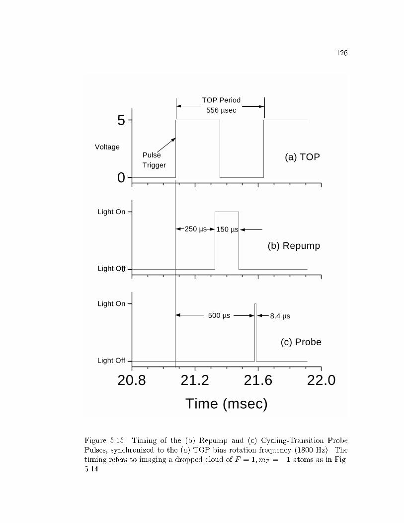
126
20.8 21.2 21.6 22.0
0
Light On
Light Off
Light Off
500 µs 8.4 µs
(c) Probe
Time (msec)
0
Light On
250 µs 150 µs
(b) Repump
0
5
PulseTrigger
TOP Period556 µsec
(a) TOPVoltage
Figure 5.15: Timing of the (b) Repump and (c) Cycling-Transition Probe
Pulses, synchronized to the (a) TOP bias rotation frequency (1800 Hz). The
timing refers to imaging a dropped cloud of F = 1; mF = �1 atoms as in Fig.
5.14

127
When the probe pulses are triggered at 21 msec we then enter into a
critical timing phase. To insure that the optical beams are parallel with the
rotating bias �eld, we synchronize the turn-on of the repump and probe beams
with the TOP �eld rotation. The repump light turns-on �rst, 250 �sec after
the �rst rising edge of the TOP trap Synch signal. The repump light is incident
on the atoms, but does not shine into the camera. The repump lasts 150 �sec
to completely pump the atoms into the F = 2 state. The probe light turns on
250 �sec later. To image the F = 2 atoms we only omit the initial ash of the
repump light.

Chapter 6
The Time-Averaged Orbiting Potential Magnetic Trap
6.1 Introduction
Magnetic trapping is a powerful technique to manipulate and con�ne
cold atoms. For many experiments, including BEC, a purely magnetic trap
circumvents the limitations which prevent the simultaneous achievement of
high densities (. 1012 atoms/cm3) and low temperatures (at or below the
recoil limit) in optical traps. The �rst magnetic trap realized for neutral atoms
was the quadrupole magnetic trap [83]. Some early experiments to achieve
BEC focused on quadrupole traps due to their simplicity, their integral nature
as part of a MOT apparatus and their tight con�nement [21, 104]. In addition,
BEC experiments need long trap lifetimes for successful evaporative cooling.
On this count, quadrupole traps fail: Atoms are ejected from the trap by
Majorana spin- ips [160] near the central zero-�eld region [21, 104]. The Time-
averaged Orbiting Potential (TOP) magnetic trap [21] successfully modi�ed
the quadrupole potential to permit long trap lifetimes and enable the �rst
observation of BEC in a dilute vapor of 87Rb [22]. Another solution to the
Majorana problem is to use a Io�e-Pritchard (IP) magnetic trap [82] which
has a non-zero magnetic �eld at its potential minimum. Shortly after the
success in the TOP trap, several experiments used a variety of di�erent IP

129
magnetic traps to achieve BEC [142, 121, 122, 161, 162]. In spite of the success
of the IP traps, TOP traps continue to be used in several BEC experiments
with 87Rb [163, 164, 165, 166] and 23Na [167], as well as experiments with 133Cs
[168, 169, 170].
Magnetic �elds can exert forces on atoms by interacting with an
atom's magnetic moment ~�. The interaction between a magnetic moment
and a magnetic �eld ~B is given by the familiar Hamiltonian H = �~� � ~B.
The potential energy of atoms that are spin aligned with the �eld increases
as the magnetic �eld increases. Thus, atoms experience a force towards lower
magnetic �elds, and by creating a local minimum in the magnetic �eld we can
con�ne these so-called \weak-�eld seeking" states. The Time-averaged Or-
biting Potential (TOP) creates a time-average minimum in a time-dependent
magnetic �eld consisting of a static spherical quadrupole magnetic �eld plus a
uniform bias �eld rotating at frequency !T [21]. The uniform �eld displaces
the zero point of the quadrupole magnetic �eld from its static position and
moves the point in a circular orbit. The TOP will con�ne the atoms as long as
two conditions on the rotation frequency of the bias �eld are satis�ed. First,
the bias �eld must rotate fast compared with the oscillation frequency ! of
atoms in the potential such that the net force of attraction of the atoms will
be towards the center of the quadrupole orbit. We call this the time-averaging
condition, which we state formally as
!T � !: (6.1a)
If the �eld rotates too quickly the magnetic moments are unable to follow the

130
�eld adiabatically. The atoms then make transitions from trapped to untrapped
spin-states. The upper bound on !T is determined by the Larmor frequency-
splitting between spin states of an atom in a magnetic �eld !L = �j ~Bj=~. We
call the upper bound on the TOP rotation frequency the adiabaticity condition,
which is formally expressed
!T � !L: (6.1b)
The subject of the present chapter is a detailed study of the properties
of, and the limitations to, the TOP magnetic trap. Historically, IP traps have
been studied in much greater detail than the TOP trap [82, 171, 92, 157, 114,
121, 152]. Very little experimental work has appeared in the literature about
the TOP trap beyond the initial demonstration [21] and its role in various BEC
experiments [22, 8, 172, 164]. There have been some theoretical treatments of
the TOP [173, 174, 175, 176, 177]. In the �rst part of this chapter we present
a detailed and improved theoretical description of the TOP that includes the
e�ects of gravity. We �nd corrections to the trap frequencies that o�er control
over the trap symmetry through the sag of atoms in the trap. The TOP is
only an approximately harmonic trap, so we also calculate anharmonic contri-
butions to the potential. We �nd that the anharmonicities of the TOP become
lower when the trap is made more spherical. We further generalize the TOP
theory for non-isotropic rotating bias �elds. In the latter section of the chapter
we present a series of measurements of the TOP trap. First, we verify the
improved theory of the TOP by precisely measuring the trap frequencies and
aspect ratios. Next, we determine limitations to TOP performance through

131
measurements of the loss of atoms from the trap when the TOP is operated in
various extremes of operation. As our �rst experiment, we studied the lifetime
of atoms in the TOP as a function of the bias �eld, from just over 6 Gauss to
a very small value of 200 mG. The low-�eld regime is particularly interesting
because recent experiments suggest that a low bias �eld trap is necessary to
observe BEC in 133Cs [178]. In our second study of extreme operation, we test
the fundamental conditions, 6.1, of the TOP by varying the rotation frequency
of the bias �eld. We measure loss of atoms from the TOP trap for a range of
rotation frequencies covering nearly three orders-of-magnitude.
6.2 Theory of the Time-Averaged Orbiting Potential
6.2.1 Basic Theory
The complete potential of a TOP Magnetic trap consists of the sum
of the total magnetic potential and the gravitational potential. Previous work
neglected the e�ects of gravity [21] but, as we will show, gravity can have
a profound in uence on the qualitative features of the trap. We begin by
brie y reproducing the results of [21] so we can later contrast them to the
results including gravity. The quadrupole magnetic �eld is cylindrically sym-
metric about an axis parallel to the vertical de�ned by gravity. We write the
quadrupole �eld, to lowest order in its spatial coordinates near the center of
the anti-Helmholtz coil pair that generates the �eld, as:
~Bq = B0
z(1
2xx +
1
2yy � zz); (6.2)

132
where B0
z is the axial magnetic �eld gradient. The bias �eld rotates in a plane
orthogonal to the axis of the quadrupole �eld that we write as:
~Bb = B0cos(!Tt)x+B0sin(!Tt)y (6.3)
where B0 is the bias �eld and !T is the angular frequency at which the bias
�eld rotates. When condition 6.1b is satis�ed, the atomic magnetic moments
~� adiabatically follow the magnetic �eld and only the magnitude of the total
�eld is important for calculating the magnetic potential energy:
Umagnetic(~r; t) = �j ~Bq + ~Bbj (6.4)
= �
r(B0
z
2x+B0cos(!Tt))2 + (
B0
z
2y +B0sin(!Tt))2 + (B0
zz)2 (6.5)
In practice the atoms are con�ned far from the rotating quadrupole
zero and very near the trap minimum at temperatures small compared with
the trap depth. In other words, the region of interest in the potential is for
distances r from the trap center small compared with the radius of the orbit of
the quadrupole zero, R � B0=B0
z=2. The radius R is the natural length scale
for the problem and we can rewrite Umagnetic in terms of r=R:
U(~r; t) = �B0
r(x
R+ cos(!Tt))2 + (
y
R+ sin(!Tt))2 + (2
z
R)2 (6.6)
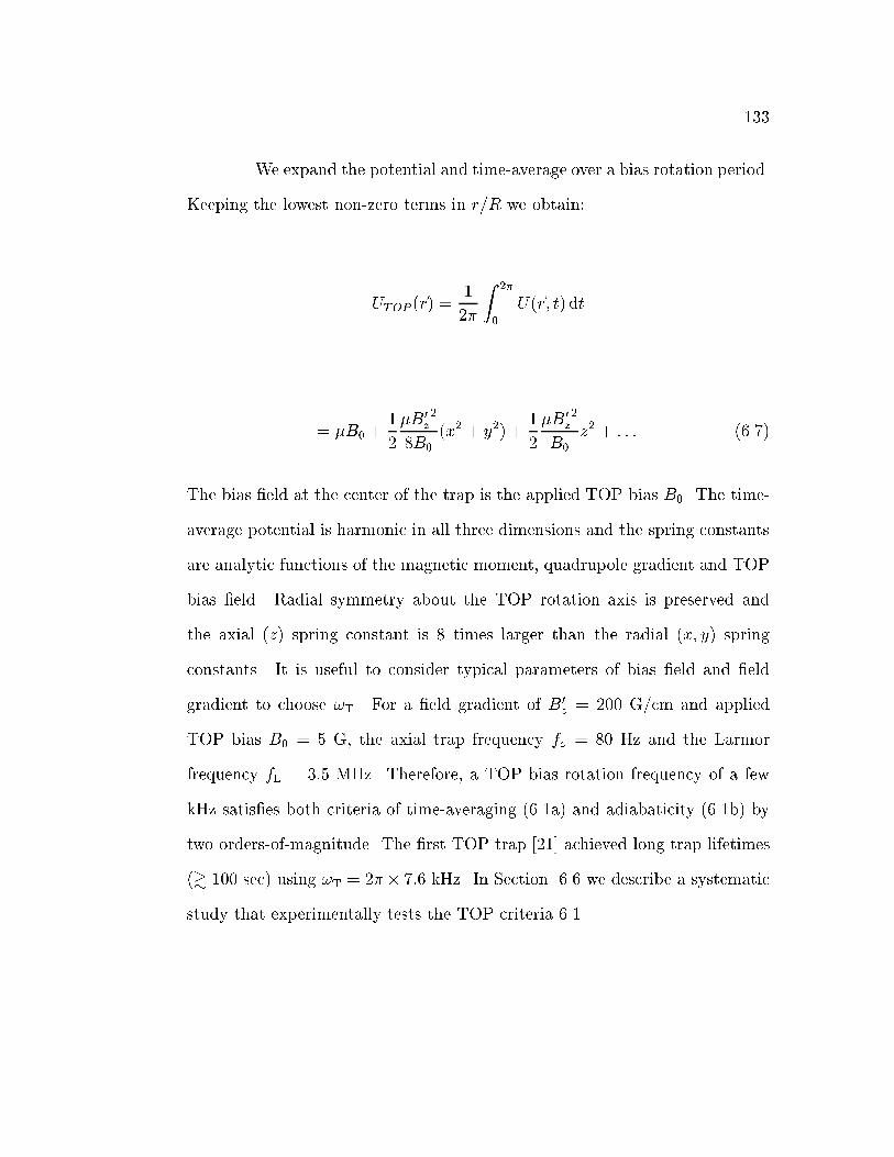
133
We expand the potential and time-average over a bias rotation period.
Keeping the lowest non-zero terms in r=R we obtain:
UTOP (~r) =1
2�
Z 2�
0
U(~r; t) dt
= �B0 +1
2
�B0
z2
8B0
(x2 + y2) +1
2
�B0
z2
B0
z2 + : : : (6.7)
The bias �eld at the center of the trap is the applied TOP bias B0. The time-
average potential is harmonic in all three dimensions and the spring constants
are analytic functions of the magnetic moment, quadrupole gradient and TOP
bias �eld. Radial symmetry about the TOP rotation axis is preserved and
the axial (z) spring constant is 8 times larger than the radial (x; y) spring
constants. It is useful to consider typical parameters of bias �eld and �eld
gradient to choose !T. For a �eld gradient of B0
z = 200 G/cm and applied
TOP bias B0 = 5 G, the axial trap frequency fz = 80 Hz and the Larmor
frequency fL = 3:5 MHz. Therefore, a TOP bias rotation frequency of a few
kHz satis�es both criteria of time-averaging (6.1a) and adiabaticity (6.1b) by
two orders-of-magnitude. The �rst TOP trap [21] achieved long trap lifetimes
(& 100 sec) using !T = 2�� 7:6 kHz. In Section 6.6 we describe a systematic
study that experimentally tests the TOP criteria 6.1.

134
6.2.2 E�ects of Gravity
The previous treatment breaks down when gravity causes the mini-
mum of the total magnetic plus gravitational potential to sag signi�cantly from
the center of the quadrupole �eld. The total potential including gravity is
U(~r; t) = �
r(B0
z
2x +B0cos(!Tt))2 + (
B0
z
2y +B0sin(!Tt))2 + (B0
zz)2 +mgz
(6.8)
where m is the mass of an atom and g is the acceleration due to gravity. The
equilibrium position for atoms is the position which minimizes U(~r; t):
~rmin = �R
2
�p1� �2
z (6.9)
For convenience I de�ne � � mg�B0
z
. Physically, � is the ratio of the weight of an
atom to the magnetic force from the axial quadrupole gradient that supports
it. We expand U(~r; t) in powers of j~r � ~rminj=R and time-average:
UTOP(~r � ~rmin) =1
2�
Z 2�
0
U(~r � ~rmin; t) dt
= �B0
p1� �2 +
1
2
�B0
z2
8B0
(1 + �2)p1� �2(x2 + y2) +
1
2
�B0
z2
B0
(1� �2)3=2z2 + : : : (6.10)

135
Several new features emerge. First, the total o�set in the potential vanishes as
the atoms sag more in the trap (� ! 1). This occurs because the potential en-
ergy due to the magnetic bias �eld is cancelled by the decrease in gravitational
potential energy as the atoms sag. Second, the potential remains harmonic to
lowest order in the axial and radial directions and is cylindrically symmetric,
but gravitational sag introduces factors depending on � into the spring con-
stants. The presence of factors like 1� �2 force the spring constants to vanish
as � ! 1. As we expect, the potential can hardly be con�ning if it cannot
support the atoms against gravity.
An even more important feature of the gravitational corrections is
that the axial and radial spring constants are not identical functions of the
quadrupole gradient. The aspect ratio is an analytical function of � = �(B0
z):
kz
kr= 8
1� �2
1 + �2(6.11)
In the limit of large gradients the trap asymmetry approaches 8 and agrees
with the calculation of Petrich, et al. [21]. By reducing B0
z, the aspect ratio
is continuously decreased towards zero as the gradient is lowered towards the
minimum to cancel gravity. The aspect ratio does not depend on the applied
TOP bias �eld although the net bias �eld, at the center of the trap, does
increase as the gradient decreases due to an increasing vertical component to
the magnetic �eld from the quadrupole �eld. The net bias �eld is B0=p1� �.
An important special value of trap symmetry occurs when � =q
79: The aspect
ratio is 1 and the TOP is spherically symmetric.

136
TOP Expansion
term coe�cient
r2(z � zmin) 4�(1� �2)(3�2 � 1)�B0
z
3
B2
0
(z � zmin)3 32�(1� �2)2
�B0
z
3
B2
0
r4 1=4(1� �2)3=2(1 + 6�2 � 15�4)�B0
z
4
B3
0
r2(z � zmin)2 8(1� �2)3=2(1� 12�2 + 15�4)
�B0
z
4
B3
0
(z � zmin)4 32(1� �2)5=2(5�2 � 1)
�B0
z
4
B3
0
Table 6.1: Higher-Order Terms in the TOP expansion
6.2.3 Anharmonicities
An important consideration for any nearly harmonic trapping po-
tential is the magnitude of anharmonicities. Anharmonic components to the
potential can impose serious systematic limitations to experiments by provid-
ing a mechanism for damping of excitation modes of a trapped cloud or the
conversion of in-trap sloshing into cloud heating. We calculated the coe�cients
of the higher-order anharmonic terms of the TOP up to the quartic terms in
the potential. See Table 6.1. Due to cylindrical symmetry the label r means
any direction perpendicular to the symmetry axis.
Reviewing the table we notice that all of the terms depend on the
trap sag through �. Terms r2z and r2z2 couple motion in the axial and radial
directions. Overall, the cubic and quartic terms introduce fractional corrections
to the harmonic trap frequency !0i in the direction i that depend on the square
of the ratio of the amplitude of oscillation Aj, in all three dimensions j = r; z,
to the radius R [179]:

137
�!=! = �A2 (6.12)
where �!=!, � and A2 are matrices de�ned by
�!=! =
0B@
!r�!0r!r
!z�!0z!z
1CA � =
0B@�rr �rz
�zr �zz
1CA A2 =
0B@
A2r
R2
A2z
R2
1CA
The �ij are dimensionless coe�cients depending on the quadrupole �eld gra-
dient through the parameter �. After straightforward, but lengthy algebra we
obtain the matrix of anharmonicity coe�cients:
� =
0B@
164
11+�2
(3 + 7�2 � 23�4 � 3�6) 14
1��2
1+�2(2� 17�2 + 9�4)
132(2� 17�2 + 9�4) �3
4(1� �2)
1CA (6.13)
Since the o�-diagonal elements are non-zero, the oscillation frequency in r (and
z) direction depends on the amplitudes of motion in both the r and z directions,
e.g. !r = !0r(1 + �rr(Ax=R)2 + �rz(Az=R)
2).
We �rst consider the o�-diagonal elements of �. These elements arise
solely from the mixing terms in the potential, r2z and r2z2. Recalling that
the trap aspect ratio is 6.11, we note that both o�-diagonal corrections to the
trap frequencies are equal for r and z oscillations of equal energy. Applying
similar reasoning, we can directly compare the fractional anharmonic frequency
shifts due to both diagonal and o�-diagonal terms. In Figure 6.1, we plot the

138
fractional anharmonic frequency corrections due to o�-diagonal and diagonal
terms, expressed in units of the square of the ratio of Ar=R, as a function of
mg=�B0
z, or �. In general, the o�-diagonal contributions are of the same order
as the diagonal elements.
Next, we are interested in the total fractional frequency shift in the
axial and radial directions, consisting of both diagonal and o�-diagonal ele-
ments. Once again, we assume equal energy of motion in all directions and
express the fractional frequency shifts in terms of the square of the ratio of
radial amplitude to R. This allows (i) evaluation of the anharmonic shifts in
a single frequency due to amplitudes of motion in both r and z directions,
and (ii) comparison of the anharmonicity shifts in axial versus radial direc-
tions. The anharmonic frequency shifts are plotted versus mg=�B0
z in Figure
6.2. The curves may be interpreted in the following way. Consider a motion in
the trap whose total energy is 3=2k0rA2r and is evenly divided among all three
dimensions. Now, for example, let Ar=R = 1, which means that the ampli-
tude of motion extends all the way to the orbit of the quadrupole zero. When
mg=�B0
z = 1, Figure 6.2 shows that the fractional shift in the axial (radial)
frequency is -0.375 (-0.3125). As expected, for an amplitude of motion far from
the center of the TOP expansion there are substantial anharmonic corrections
to the trap frequencies.
The changes in trap symmetry and anharmonicity di�er slightly from
previous experience with IP magnetic traps. Changing the IP trap symmetry
from highly asymmetric with cylindrical symmetry to nearly symmetric usu-
ally comes with two prices. First, a large bias �eld is required to reduce the
larger spring constant. Second, the anharmonicities in all directions worsen,
often quite substantially. In contrast, the TOP trap aspect ratio tunes only

139
0.0 0.2 0.4 0.6 0.8 1.0-0.2
-0.1
0.0
0.1
off-diagonal diagonal, axial diagonal, radial
∆ω i
j / ω
i (
A2 ra
dial /
R2 )
mg / µB'z
Figure 6.1: Comparison of the diagonal radial (�!rr=!r, solid line), diagonal
axial (�!zz=!z, dashed line) and o�-diagonal (�!ij=!i, where i 6= j, dotted
line) contributions to the fractional anharmonic frequency shift, as a function
of mg=�B0
z, the ratio of atom weight to magnetic force. In general, �!mn =
!m � !0m, where !0m is the zero-amplitude oscillation frequency in the mth
direction. We assume the same energy of motion in axial and radial directions
and express the fractional frequency shift in terms of the ratio A2r=R
2, where
the Ar is the radial oscillation amplitude and R is the orbital radius of the
quadrupole zero.

140
0.0 0.2 0.4 0.6 0.8 1.0-0.4
-0.3
-0.2
-0.1
0.0
0.1
radial axial
SphericalSymmetry
∆ω /
ω (
A2 ra
dial /
R2 )
mg / µB'z
Figure 6.2: Plot of the fractional shift, !i � !0i=!0i in the axial (i=z, dashed
line) and radial (i=r, solid line) trap frequencies as a function of mg=�B0
z,
the ratio of atom weight to magnetic force. To facilitate comparison of axial
and radial frequency shifts, we assume the same energy of motion in axial and
radial directions and express the fractional frequency shift in terms of the ratio
A2r=R
2, where the Ar is the radial oscillation amplitude and R is the orbital
radius of the quadrupole zero. The solid, vertical line indicates where the
TOP has spherical symmetry (the zero-amplitude axial and radial frequencies
are equal).

141
with the gradient. The net bias is a�ected, but as a second-order e�ect of the
gradient. Regarding anharmonicities in the TOP, the above discussion shows
that the magnitude of the fractional frequency shift generally increases as we
decrease the quadrupole gradient and make the potential spherical. The frac-
tional shift, however, is unchanged by the applied TOP �eld as long as the
ratio Ar=R is constant. It is also important to point out the magnitude of the
fractional frequency shift can be quite small. For the worst anharmonicities,
when � = 1, oscillation amplitudes less than 1=10R su�er less than a 1% frac-
tional frequency shift. This is a typical ratio of radial condensate size to R,
under reasonable experimental conditions.
6.2.4 E�ect of Eccentricity on the TOP Trap
When the rotating bias �eld of the TOP is not radially symmetric
several corrections occur to the TOP frequencies. Breaking of radial symmetry
may be characterized as an eccentricity e in the path of the quadrupole zero
point. Eccentricity is almost unavoidable in a laboratory TOP trap because
making a bias �eld that rotates with the same magnitude in all directions to
better than 5% is di�cult. Broken radial symmetry can subsequently alter the
physics of excitations of trapped atom clouds or Bose-Einstein Condensates
[8, 141]. Eccentricity also provides a tool for inducing excitations of various
symmetries into a trapped atom cloud [180].
Consider a TOP trap in which the bias �eld in the y direction is e
times larger in the x direction, i.e. B0x = B0 and B0y = eB0. The rotating
�eld becomes:

142
~Bb = B0cos(!T t)x + eB0sin(!T t)y (6.14)
For simplicity, we assume a large axial �eld gradient so we can ignore the sag
due to gravity and the gravitational potential. The simpli�ed total potential
is
Umagnetic(~r; t) = �
r(B0
z
2x+B0cos(!T t))2 + (
B0
z
2y + eB0sin(!T t))2 + (B0
zz)2
(6.15)
due to the combination of eccentric rotating �eld and the static quadrupole
potential. As before, we expand the potential about its minimum (~rmin = 0)
and retain terms to second-order in j~rj=R. The eccentricity obviously breaks
the cylindrical symmetry of the potential such that the time-averaged spring
constants are not analytical functions of e. We numerically integrate the po-
tential over a bias rotation period to obtain the time-averaged bias �eld and
spring constants. We are interested in the dependence of symmetry breaking
between the x and y spring constants on the eccentricity of the bias �eld. A
complicating e�ect is that increasing e > 1 also increases the time-averaged
magnetic �eld. We remove this complication by calculating the ratio of the
y frequency to the x frequency so that the overt �eld-dependence of the fre-
quencies cancel. The frequency ratio as a function of eccentricity is plotted
in Figure 6.3. As the �eld along y increases relative to the �eld along x, the
frequency along y decreases relative to the frequency along x. The dependence
on eccentricity is rather slow: when By is 50% larger than Bx (e = 1:5), !y is

143
only 10% smaller than !x. The weak dependence of !y=!x on e is also evident
in an analytical expansion in the limit of small eccentricity:
!x = (1 +1
4e)!y: (6.16)
We are also interested in knowing if the eccentricity changes the ratio
of the axial frequency to the radial frequencies. A calculation of the ratio of
!z to the mean radial frequency (!x + !y)=2 shows that the ratio is equal top8 for all values of e. This is precisely the ratio expected for a cylindrically
symmetric TOP with no eccentricity.
The insensitivity of the ratio of \radial" frequencies to the eccentricity
is useful for ensuring near-cylindrical symmetry in the TOP trap. The isotropy
of bias �eld in the rotation plane is typically no better than 5 � 10%. How-
ever, from Figure 6.3 and Equation 6.16 we note that the corresponding radial
frequencies are split by no more than 1:25 � 2:5%. In the opposite extreme
of large eccentricity, the frequency splitting can be very large (25% at e = 3)
without a fundamental breakdown of the TOP trap.
6.3 Experimental Method
We experimentally study the TOP magnetic trap by creating cold
clouds of 87Rb in a double-MOT apparatus and observing the behavior of the
atomic velocity distributions. We will only review the apparatus as details are
given elsewhere [172]. See also Chapter 5. A high-pressure (� 10�9 Torr)
vapor cell MOT creates ensembles of several 108 atoms that are pushed with
a resonant laser pulse into a second MOT maintained in a glass cell at very

144
1.0 1.5 2.0 2.5 3.00.75
0.80
0.85
0.90
0.95
1.00
2By
2Bxω
y / ω
x
Eccentricity (By / Bx)
Figure 6.3: Ratio of y to x \radial" trap frequencies in an eccentric TOP trap.

145
low vapor pressure (� 10�11 Torr). After twenty to thirty pulsed loading
cycles, 109 atoms are optically compressed (CMOT) and cooled (molasses) in
preparation for loading into a purely magnetic trap. The atoms are optically
pumped into the 5S1=2F = 1; mF = �1 (F = 1) state of 87Rb and the magnetic
�elds for the TOP trap are turned-on. The spring constants of the magnetic
trap are adiabatically ramped-up and a radio-frequency (rf) magnetic �eld is
ramped-down in frequency to perform evaporative cooling. The �nal value
of the rf frequency determines the �nal cloud temperature. After attaining
a cloud of desired temperature and density using a standard con�guration of
magnetic �elds and rf frequencies, we adiabatically ramp the trap to a new set
of trap parameters (net bias �eld, amount of sag, frequency, etc.) and conduct
experiments for an interaction and wait time (lasting tens of milliseconds to
minutes). Exact details of this penultimate stage are described in the following
experimental sections. After the interaction and wait, the atoms are released
from the trap and ballistically expand for typically 21 msec. The expanded
and dropped cloud is optically pumped from the F = 1 into the 5S1=2F = 2
ground-state and probed with an 8 �s pulse of light at a frequency tuned near
the 5S1=2F = 2; mF = 2 ! 5P3=2F = 3; mF = 3 cycling transition. The
release and absorption imaging destroys the cloud. The absorption shadow
of the atoms is imaged onto a CCD array and �t to a Gaussian, inverted
parabola or double-Gaussian distribution function depending on if the atom
cloud is a noncondensed gas, pure BEC, or a mixture of noncondensed and
quantum degenerate gases, respectively. From the �ts to the 2-D velocity
distributions we extract all the relevant information about the sample: Total
number, number in the condensate, temperature and position [13].

146
6.4 Trap Frequency and Symmetry Measurements
Accurate knowledge of trap parameters is crucial for extracting quan-
titative information from experiments with trapped particles. Nearly every
physical parameter of interest { temperature, density, phase space density, size
of ground state, etc. { is connected to knowledge of the trap frequencies. For
example, the temperature of a classical gas is obtained from knowing the root-
mean-square size of the gas in the trap and the trap frequency. In the following
section we describe measurements of the frequency of oscillation of atoms in
the TOP trap and the spatial symmetry of the trap. We compare these data
to the improved theory of the TOP frequencies.
We measure trap frequency by exciting small-amplitude oscillations
of our smallest clouds in the trap, recording the cloud's center-of-mass (CM)
position versus time, and �tting the data to a single-frequency sine wave. We
�rst create pure condensates as described above and then ramp the TOP to a
particular �eld gradient and bias �eld. CM oscillations of the BEC are created
in two complementary ways. First, an axial (vertical) CM oscillation is in-
duced using a �eld ramp that is slightly non-adiabatic, causing a vertical slosh
of the cloud as the atoms suddenly sag against gravity. Second, a radial CM
oscillation is induced by a magnetic �eld applied for several msec with a cur-
rent pulse through a small, horizontally-oriented coil. We minimize systematic
shifts in the oscillation frequency due to anharmonicities by using pure BECs
(our smallest clouds) and small excitation amplitudes (� 1=10R) After the
�eld ramp and horizontal push initiate the CM motion, the atom cloud freely
oscillates in the trap for a variable delay time. Immediately following the delay
we image the atoms. By repeating the cycle of cloud creation and CM excita-

147
tion, for varying free oscillation times, we generate a plot of the CM position
versus time that is �t to a single-frequency sine wave. The �t frequency is the
oscillation frequency of the trap in the direction of CM oscillation.
Typical CM oscillation data is shown in Figure 6.4 for the axial (6.4a)
and radial (6.4b) oscillations. Each pair of axial and radial center positions
at each time correspond to a single measurement cycle. The data for both
directions are well �t by a single frequency sine wave. The frequencies are
fz = 12:1 � 0:1 and fx = 13:0 � 0:1 Hz. The error bars are limited by the
statistical uncertainty of the �tting [181]. Finally, we point-out that for the
trap parameters chosen (B0 = 540 mG, B0
z = 34 G/cm) we observe a dramatic
change in the trap aspect ratio from thep8 value predicted for the TOP trap
in the absence of gravity.
We examine the theory of TOP operation, in the limit of small ax-
ial quadrupole gradients, by �xing the magnitude of the rotating bias �eld to
B0 = 540 mG and varying the axial �eld gradient to change the trap frequency
and symmetry. For each �eld gradient we measure both axial and radial trap
frequencies. The data are plotted in Figure 6.5. The error bars on each fre-
quency point are smaller than the points on the graph. At high gradients, the
axial frequencies are greater than 200 Hz. The radial frequencies are notice-
ably smaller at the same large gradients. Decreasing the �eld gradient causes
the axial frequency to decrease much more rapidly than the radial frequency,
until at B0
z = 36 G/cm the radial frequency (13.0 Hz) is larger than the axial
frequency (12.1 Hz). The frequency data are �t to functional forms for the
frequency given in Eq. (6.10) for the axial and radial directions, with two �t
parameters corresponding to the �eld gradient and bias �eld calibrations to
the control voltages. The excellent �t to the data veri�es the accuracy of the

148
0 100 200 300 400250
300
350
400
450fx = 13.0(1) Hz, amplitude = 70 µm
Rad
ial C
ente
r ( µ
m)
Time (ms)
0 100 200 300 400
350
400
450
500
fz = 12.2(1) Hz, amplitude = 75 µm
Axi
al C
ente
r ( µ
m)
Figure 6.4: Center-of-mass oscillations of atoms in the TOP magnetic trap for
BTOP = 0:54G and B0
z = 34 G/cm.

149
improved TOP theory. By assuming the functional forms for the frequency are
correct, the �ts calibrate both �eld gradient and bias �eld to a few percent. We
can simultaneously and accurately calibrate both trap �elds because the trap
frequencies vanish rapidly at a speci�c axial �eld gradient (30:6 G/cm for the
F = 1 state). The low-gradient dependence of the trap frequencies therefore
strongly constrains the �eld gradient parameter, while the overall range of trap
frequencies dictates the size of the magnetic bias parameter.
We now focus on the change of the trap symmetry with �eld gra-
dient by plotting the ratio of the axial to radial frequencies versus the axial
�eld gradient in Figure 6.6. At large �eld gradients, we expect that the ratio
approaches the \gravity-free" limit ofp8 shown by the black horizontal line.
As the gradient decreases, the measured frequency ratios decrease from nearlyp8 (axially symmetric) to below 1 (spherically symmetric). Also plotted on
the graph is Eq. (6.11) representing the expected dependence of the frequency
ratio on the gradient. Using the gradient calibration from the �t to the data
in Figure 6.5, Eq. (6.11) is in very good agreement with the data. The lowest
frequency ratio !z=!x = 4:5=9:4 = 0:48 demonstrates that we can tune near
and around the interesting case of spherical trap symmetry. By further reduc-
ing the TOP bias �eld we can increase the spherical trap frequencies, reaching
up to 27 Hz for a bias �eld of 250 mG.
6.5 The TOP trap at Low Magnetic Bias �elds
In our next experiments we study the behavior of the TOP trap at low
magnetic bias �elds. We cite two principle motivations for why operation at
low bias �elds is interesting for both IP and TOP magnetic traps. First, small

150
20 100 2003
10
100
300
axial radial
Tra
p F
requ
ency
(H
z)
Axial Quadrupole Gradient(G/cm)
Figure 6.5: TOP Trap frequencies in the axial and radial directions as a func-
tion of axial quadrupole gradient. The rotating bias �eld is 0.54 Gauss for all
the data.

151
40 80 120 160 200
0.5
1.0
1.5
2.0
2.5
3.0
spherical trap
gravity-free limit
Fre
quen
cy R
atio
Axial Quadrupole Gradient(G/cm)
Figure 6.6: Ratio of the axial to radial trap frequencies, shown in Figure 6.5,
as a function of axial quadrupole gradient. The solid, horizontal line atp8 is
the frequency ratio in the absence of gravitational sag. The curved line is the
analytical form for the TOP symmetry, Eq. 6.11
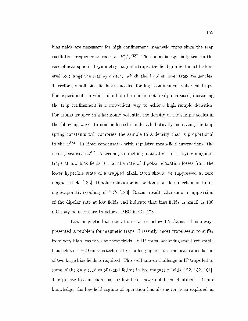
152
bias �elds are necessary for high con�nement magnetic traps since the trap
oscillation frequency ! scales as B0
z=pB0. This point is especially true in the
case of near-spherical symmetry magnetic traps: the �eld gradient must be low-
ered to change the trap symmetry, which also implies lower trap frequencies.
Therefore, small bias �elds are needed for high-con�nement spherical traps.
For experiments in which number of atoms is not easily increased, increasing
the trap con�nement is a convenient way to achieve high sample densities.
For atoms trapped in a harmonic potential the density of the sample scales in
the following ways. In noncondensed clouds, adiabatically increasing the trap
spring constants will compress the sample to a density that is proportional
to the !3=2. In Bose condensates with repulsive mean-�eld interactions, the
density scales as !6=5. A second, compelling motivation for studying magnetic
traps at low bias �elds is that the rate of dipolar relaxation losses from the
lower hyper�ne state of a trapped alkali atom should be suppressed at zero
magnetic �eld [182]. Dipolar relaxation is the dominant loss mechanism limit-
ing evaporative cooling of 133Cs [183]. Recent results also show a suppression
of the dipolar rate at low �elds and indicate that bias �elds as small as 100
mG may be necessary to achieve BEC in Cs [178].
Low magnetic bias operation { at or below 1-2 Gauss { has always
presented a problem for magnetic traps. Presently, most traps seem to su�er
from very high loss rates at these �elds. In IP traps, achieving small yet stable
bias �elds of 1�2 Gauss is technically challenging because the near-cancellation
of two large bias �elds is required. This well-known challenge in IP traps led to
some of the only studies of trap lifetime in low magnetic �elds [122, 152, 161].
The precise loss mechanisms for low �elds have not been identi�ed. To our
knowledge, the low-�eld regime of operation has also never been explored in
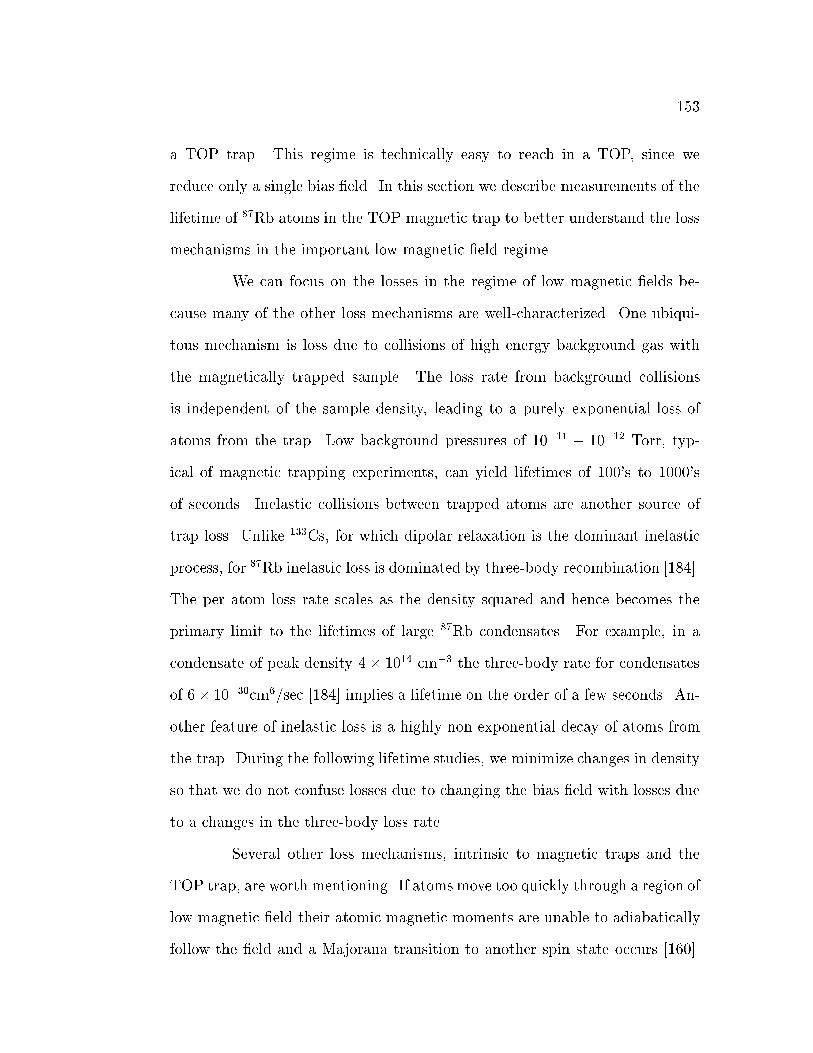
153
a TOP trap. This regime is technically easy to reach in a TOP, since we
reduce only a single bias �eld. In this section we describe measurements of the
lifetime of 87Rb atoms in the TOP magnetic trap to better understand the loss
mechanisms in the important low magnetic �eld regime.
We can focus on the losses in the regime of low magnetic �elds be-
cause many of the other loss mechanisms are well-characterized. One ubiqui-
tous mechanism is loss due to collisions of high energy background gas with
the magnetically trapped sample. The loss rate from background collisions
is independent of the sample density, leading to a purely exponential loss of
atoms from the trap. Low background pressures of 10�11 � 10�12 Torr, typ-
ical of magnetic trapping experiments, can yield lifetimes of 100's to 1000's
of seconds. Inelastic collisions between trapped atoms are another source of
trap loss. Unlike 133Cs, for which dipolar relaxation is the dominant inelastic
process, for 87Rb inelastic loss is dominated by three-body recombination [184].
The per atom loss rate scales as the density squared and hence becomes the
primary limit to the lifetimes of large 87Rb condensates. For example, in a
condensate of peak density 4� 1014 cm�3 the three-body rate for condensates
of 6� 10�30cm6/sec [184] implies a lifetime on the order of a few seconds. An-
other feature of inelastic loss is a highly non-exponential decay of atoms from
the trap. During the following lifetime studies, we minimize changes in density
so that we do not confuse losses due to changing the bias �eld with losses due
to a changes in the three-body loss rate.
Several other loss mechanisms, intrinsic to magnetic traps and the
TOP trap, are worth mentioning. If atoms move too quickly through a region of
low magnetic �eld their atomic magnetic moments are unable to adiabatically
follow the �eld and a Majorana transition to another spin state occurs [160].

154
The change of spin alignment and/or the gain of kinetic energy leads to trap
loss. Majorana transitions occur when the rate of change of the magnetic �eld
seen by the atom is comparable to the Larmor splitting between magnetic
spin states: ~v � ~r� ~BB
�� �B
~. For the temperatures and �eld gradients of our
experiments, this condition is met for magnetic �elds of only a few mG and
are much smaller than the �elds we study.
Another concern relating to trap loss is that the TOP trap has a
�nite energy depth Ed, de�ned by the radius R at which the quadrupole zero
orbits the atoms. The trap depth Ed = kBTd = �B=4 decreases as the bias
�eld decreases. Atoms with energy greater than or equal to the trap depth
encounter the quadrupole zero, undergo a spin- ip and are lost from the trap
at a rate on the order of the radial oscillation frequency. The fraction of a cloud
of atoms that is lost in this way is determined by the fraction of atoms with an
energy larger than the trap depth. For example, in a non-condensed gas 65%
of the sample is lost in a few radial oscillation periods if the trap depth is equal
to the mean energy of the cloud (3kBT ). If the trap depth is twice the cloud's
mean energy then only about 11% are lost in a similar time. Twice the mean
energy, 6kBT , therefore is a useful, approximate de�nition of the maximum
energy of atoms con�ned in the TOP trap. Equating 6kBT to the trap depth
Ed, we estimate the maximum temperature of an atom cloud in the TOP trap.
At a bias �eld of 1 Gauss, the trap depth for F = 1 (� = 1=2�B) atoms is 8:3
�K and implies a maximum temperature for the trapped atoms of < 1:4 �K.
A �nal concern are trap losses from magnetic �eld noise, coming from
an ambient source, a frequency component of the magnetic �eld current, or
both sources. Noise power at frequencies twice the trap frequencies (10-100's
of Hz) can parametrically drive the sample and eventually heat atoms out of

155
the trap [185]. At higher frequencies, noise power at hundreds of kHz can
directly drive spin- ip transitions.
In our �rst experiments we measured loss of atoms from noncondensed
clouds (Figure 6.7). Generally, we observe atom loss that is well-�t by an
exponential decay in the number of atoms. We therefore ascribe a 1=e lifetime
to the atom loss, that is the inverse of the exponential decay rate derived from
a �t to the data. Starting in the trap with 6.2 Gauss bias �eld we observe a
lifetime of 348 sec, consistent with losses due to collisions with background gas.
The lifetime decreases linearly with decreasing bias �eld in the trap, reaching 94
sec at 1.1 Gauss. Below 1 Gauss, the lifetime drops more quickly with the �eld
and reaches 0.5 sec at 190 mG. Although the cloud density increases slightly
as the bias �eld decreases, the loss rates are too fast to be explained by three-
body recombination. We also examined the trap depth as a loss mechanism.
A plot of the ratio of trap depth Ed = kBTd to the initial mean energy 3kBT
as a function of trap bias (Figure 6.8, solid squares) shows that the TOP is
shallower with respect to the mean particle energy at low bias �elds. We also
�nd heating of the atoms while they reside in the trap, further narrowing the
di�erence between trap depth and mean energy. The heating rate is initially
5 � 10 nK/sec and vanishes as the cloud reaches a steady-state temperature.
The time-scale for reaching the steady-state on the order of the 1=e lifetime.
Heating from a shallow trap might explain the very short lifetimes in the 190,
350 and 650 mG traps, where heating leaves the trap depth only 1.3, 2.9 and
3.3 times larger than the mean energy of atoms, for long dwell-times in the
trap (Figure 6.8, hollow circles). However, this mechanism seems unlikely to
be the loss mechanism for all the data. Above 1 Gauss, where the trap depth is
larger than four times the mean energy (after heating), a loss mechanism due
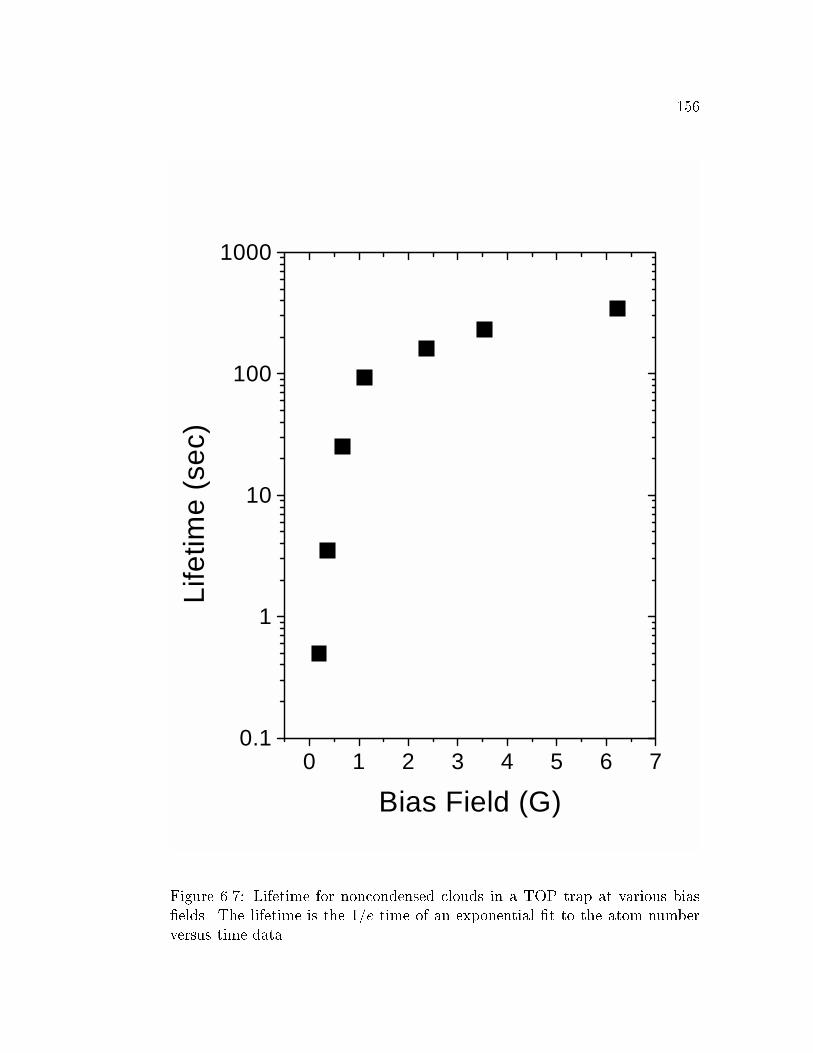
156
0 1 2 3 4 5 6 70.1
1
10
100
1000
Life
time
(sec
)
Bias Field (G)
Figure 6.7: Lifetime for noncondensed clouds in a TOP trap at various bias
�elds. The lifetime is the 1=e time of an exponential �t to the atom number
versus time data.

157
0 1 2 3 4 5 6 71
10
100
Trap Depth / Mean Energy:
initial cloud cloud after heating
Tra
p D
epth
/ 3k
BT
Bias Field (G)
Figure 6.8: Ratio of trap depth to mean cloud energy for noncondensed clouds
in a TOP trap at the same bias �elds used to study lifetimes (see Fig. 6.7). The
squares and hollow circles show the ratio of trap depth to mean cloud energy,
Ed=3kBT , for clouds initially in the trap and after a steady-state temperature
is reached due to heating, respectively. Ed is de�ned in the text.

158
to heating should exhibit a very non-exponential loss pro�le. In these cases, in
which mean energy is much less than the trap depth, a �nite time is required
to heat the atoms before their mean energy is comparable to the trap depth,
at which point the loss is subsequently exponential. We neither observe this
delay nor non-exponential character to our atom loss pro�les.
At this point we exploit some features of the Bose condensate to bet-
ter understand the loss physics. The maximum extent of a large (106 atom),
pure condensate is 2�3 times smaller than the full-width half maximum of non-
condensed (Gaussian pro�le) clouds just above the BEC transition. The con-
densate density pro�le for our experiments is well-approximated by an inverted
paraboloid which has a sharp spatial cut-o� in the density pro�le, de�ned by
the half-width at zero maximum (hwom) of the distribution. Therefore, the
probability of a condensate atom encountering the zero of the quadrupole �eld,
and hence being lost from the trap, is negligible if R < Xhwom. We created
condensates with temperatures T < 0:4Tc and measured their lifetime in the
trap. Our �rst measurements of the condensate lifetimes, for bias �elds larger
than 1 Gauss, displayed a surprising linear decay of number with time. For
these samples the condensate decays into a broad non-condensed cloud, which
also decays in time. The decay of a condensate in a TOP trap of bias �eld 6.2
Gauss is shown in Fig. 6.9 (solid squares). The cloud has an initial central
density of 7:3� 1013 atoms/cm3, from which we predict an initial three-body
limited lifetime of 86 sec. The observed 1=e time of the linear decay is only
12 sec. Our previous experience with similar loss behavior [152] suggested
that atoms heated out of the condensate nonetheless remain trapped, albeit
at higher energy, and enhance the loss rate by continuing to collide with the
remaining condensate atoms. We quench the loss-inducing collisions by ap-

159
plying a weak rf magnetic �eld tuned to an energy lying at or just inside the
orbit of the rotating zero-�eld. This so-called \rf shield" induces spin- ip of
hot atoms before they return to knock atoms from the condensate. The shield
lies at high enough energy that the initial condensate number is una�ected,
but the e�ect on the loss of atoms is dramatic. The decay pro�le becomes
well-�t by an exponential curve with a much longer 1=e lifetime than without
the rf shield. At 6.2 Gauss the lifetime, as extracted by an exponential �t to
the data (dashed line in Fig. 6.9), jumps to 67 sec, consistent with losses due
to background collisions (� 400 sec) and 3-body recombination [186].
We measured lifetimes of pure condensates over the same range of bias
�elds we studied with noncondensed clouds and applying an rf shield. The data
are shown in Figure 6.10. The lifetimes are determined by �tting exponential
decay curves to the data. The condensate lifetime decreases as the bias �eld
decreases. For bias �elds larger than 1 Gauss, the data are reasonably �t by a
linear function of the bias �eld that is constrained to intercept the origin (we
expect no atoms to remain in the TOP at zero magnetic �eld). For bias �elds
less than 1 Gauss, the lifetimes are consistently shorter than the linear �t.
We note that, even with the rf shield, only the data at 6.2 and 3.5 Gauss are
quantitatively consistent with a three-body recombination. As the bias �eld
is decreased, the e�ect of the rf shield also diminishes, until below 1 Gauss it
provides no enhancement to the condensate lifetime. Nonetheless, the loss of
atoms remains exponential for bias �elds below 1 Gauss. Also qualitatively
speaking, three-body recombination alone cannot explain the observed loss.
Over the range of bias �elds studied, the density increases a factor of two
(Fig. 6.11, empty circles), implying a factor of four change in the loss rate
due to recombination. The observed change in lifetime is a factor of 180.

160
0 40 80 120
1
10
BTOP
= 6.2 G rf shield no shield
BE
C N
umbe
r (1
05 )
Time (sec)
Figure 6.9: Decay of a Bose condensate in a TOP trap with bias �eld of
6.2 Gauss. Condensate decay was �rst measured without an rf shield (solid
squares). The data are �t to a decay curve in which the number of atoms
decreases linearly in time (solid curve). The 1=e decay time, obtained from the
linear �t, is 12 sec. Next, condensate decay was measured using an rf shield
(empty circles). The loss rate decreases dramatically and the data are well-�t
by an exponential decay curve. From the �t to the shielded data we extract a
1=e lifetime of 67 sec.

161
0 1 2 3 4 5 60.1
1
10
100
Con
dens
ate
Life
time
(sec
)
Bias Field (G)
Figure 6.10: Lifetimes of Bose condensates in a TOP trap for various bias �elds.
The error bars are purely statistical, based on exponential �ts to the observed
number vs. time decays. The data are �t to a linear function of the bias �eld
in which the lifetime is constrained to vanish when B = 0, as anticipated for
the TOP.

162
Two additional observations argue against a general density-dependent loss
that depends on magnetic �eld. First, at the same value of central density we
measure two very di�erent lifetimes (see Fig. 6.11). For example, at 9� 1013
atoms/cm3 (and at 15� 1013 atoms/cm3) we measure two lifetimes that di�er
by a factor of 3:2 (4:6). Second, as the bias �eld decreases, both condensate
and non-condensate lifetimes converge to the same values (0:4� 0:5 sec at 0.2
Gauss, see Figs. 6.7 and 6.10 ) even though the condensate central density is
an order of magnitude larger than the non-condensate. We also dismiss trap
depth as the mechanism for the decreasing condensate lifetimes. As seen in
Fig. 6.11 (solid squares) the radius of the orbit of the quadrupole zero is never
closer than 4.5 times the radial hwom (at the lowest bias �eld of 220 mG) and
is usually much larger.
Another candidate to explain the trap loss is magnetic �eld noise. The
�rst possible mechanism is that noise features near twice the trap frequencies
parametrically heat atoms out of the trap. We �nd no correlation between
reduced trap lifetime and coincidences of twice our trap frequencies with the
closest noise features at 60 and 120 Hz. The axial trap frequency is 32 Hz at
6.2 Gauss and increases with decreasing �eld to 45 Hz at 0.23 Gauss. We note
that the longest lifetime (67 sec) is observed for the axial frequency nearest
the 60 Hz feature. In the radial direction, trap frequencies start at 13 Hz (6.2
G) and also increase with decreasing �eld up to 33 Hz (0.23 G). The low �eld
lifetimes are near the 60 Hz noise, but the decrease in lifetimes begins for radial
frequencies much smaller than 60 Hz and well outside its spectral bandwidth.
Thus, parametric driving of atoms out of the trap appears unlikely.
Magnetic �eld noise at hundreds of kHz, which drives transitions in
trapped atoms into untrapped spin states, is a more likely candidate for low-

163
0 10 20 30 400.1
1
10
100
vs. R / Xhwom
Con
dens
ate
Life
time
(sec
)
R / Xhwom
6 8 10 12 14 16
vs. Central Density
Central Density (1013 cm-3)
Figure 6.11: Lifetimes of Bose condensates in a TOP trap versus the ratio
of quadrupole orbit radius to radial half-width at zero maximum (hwom),
R=Xhwom (solid squares), and versus central density (hollow circles), for the
data in Fig.6.10.

164
�eld loss. The danger of losses at these frequencies arises because the Larmor
frequency splitting between Zeeman levels is 700 kHz at 1 Gauss, and reduces
linearly with the bias �eld. We measure the magnetic �eld power spectrum by
directly monitoring, on a spectrum analyzer, the voltage induced in a pick-up
coil. The coil is placed near the trap region and oriented perpendicular to the
axis of the quadrupole coils. When only the quadrupole coils are on, we noticed
that the magnetic �eld noise spectrum exhibits a comb of noise spikes spaced
by � 20 kHz, beginning at 20 kHz and rolling-o� in amplitude above 1 MHz.
These features originate from the switching power supply for the quadrupole
coils. However, noise on the quadrupole current should be greatly suppressed
in the �eld at the center of the anti-Helmholtz coil pair because the quadrupole
coils are connected in series and so current noise cancels. Indeed, reducing the
noise spikes by 10 � 20 dB, using a less noisy power supply, did not improve
the lifetimes or the trend of reduced lifetime with reduced bias �eld. Only by
generating an arti�cial noise comb of the same frequencies with substantially
more power could we cause a reduction of trap lifetime.
Next we turned to the �eld noise associated with the TOP �eld. We
measure the power spectrum of the magnetic �eld near the cell when the TOP
coils are on, the quadrupole coils o�, and without any rotating bias �eld. Using
the same technique as above, we measure broad-band spectral noise that we
estimate is 0:7 �G=pHz at 100 kHz, rolling-o� roughly as 1/frequency3 and
hitting the noise oor of the spectrum analyzer at 800 kHz (see Fig. 6.12)
[187]. Herein lies another possible loss mechanism: As the bias �eld of the
trap is reduced, the Larmor frequency is tuned into resonance with the broad-
band noise �eld. We estimate the loss rate of atoms from the cloud with the
following model. We �rst calculate the rate at which a broad-band magnetic

165
�eld drives an atom from the trapped F = 1; mF = �1 state into the untrapped
F = 1; mF = 0 state of 87Rb using time-independent perturbation theory. The
rate may be expressed in terms of the power spectral density of the magnetic
�eld and is written as:
=�
4
��
~
�2
S(!) (6.17)
where � is the magnetic moment of the initial state, S(!) is the one-sided
power spectrum given by
S(!) =2
�
Z1
0
cos(!�)hB(t)B(t+ �)i d� .
and the correlation function of the magnetic �eld uctuations is [188]
hB(t)B(t + �)i � 1
T
Z T
0
B(T )B(T + �) dt
The loss rate for the entire sample is found by integrating the per
atom loss rate over the condensate density pro�le. The span of frequencies
covered by the condensate is so small that to an excellent approximation the
power spectrum is constant across the cloud. The rate equation is therefore:
dN
dt= ��
4
��
~
�2
S(!)N (6.18)
The frequency ! is determined by the splitting between Zeeman levels of the
F = 1 manifold, which is set by the magnetic bias �eld of the trap [189]. The

166
0 1000 2000 3000 400010
-4
10-3
10-2
10-1
100
101
P
ower
Spe
ctru
m (
µG/H
z1/2 )
Frequency (kHz)
Figure 6.12: Measurement of the �eld noise from the TOP coils at the loca-
tion of the trapped atoms. The �eld noise, in �G/pHz, rolls-o� roughly as
1/frequency3 until it reaches the noise oor of the rf spectrum analyzer at 800
kHz. Above 800 kHz, the plotted noise spectrum is an upper-estimate to the
actual �eld noise.

167
rate equation describes a purely exponential loss whose rate is proportional to
the power spectral density S(!) of the magnetic �eld noise. In our data we
also observe exponential decays, as well as increased losses for level-splitting
frequencies where the power spectral density is measured to increase. We make
a quantitative comparison to our data by modeling the overall loss rate as the
sum in parallel of the initial three-body recombination rate, a background
collision rate (0.0029 sec�1) and the noise-induced loss rate [190]. The results
of the model are compared to the measured lifetimes in Figure 6.13. The
model (solid line) closely resembles the lifetime data at very low bias �elds,
but underestimates the loss rate for much of our data. At low �elds this
is due to the rapid roll-o� in the spectral noise density S(!), which greatly
reduces the noise-induced loss rate (dashed-dotted line) above 0:2 Gauss. By
about 0.4 Gauss, three-body recombination is the predominant loss mechanism,
in the model. The model agrees well with the measured lifetimes above 3
Gauss. Given the di�culty of measuring absolute �eld noise at the atoms
a quantitative disagreement is not surprising. Unfortunately, even assuming
twice the measured �eld noise, an increased noise-induced rate (dotted line)
does not signi�cantly improve the agreement of the theory to most of the
data. The results of the model do suggest that broad-band noise-induced losses
may be a signi�cant loss mechanism at very low magnetic �elds. A detailed
understanding of the observed trap loss for all magnetic �elds requires further
study.
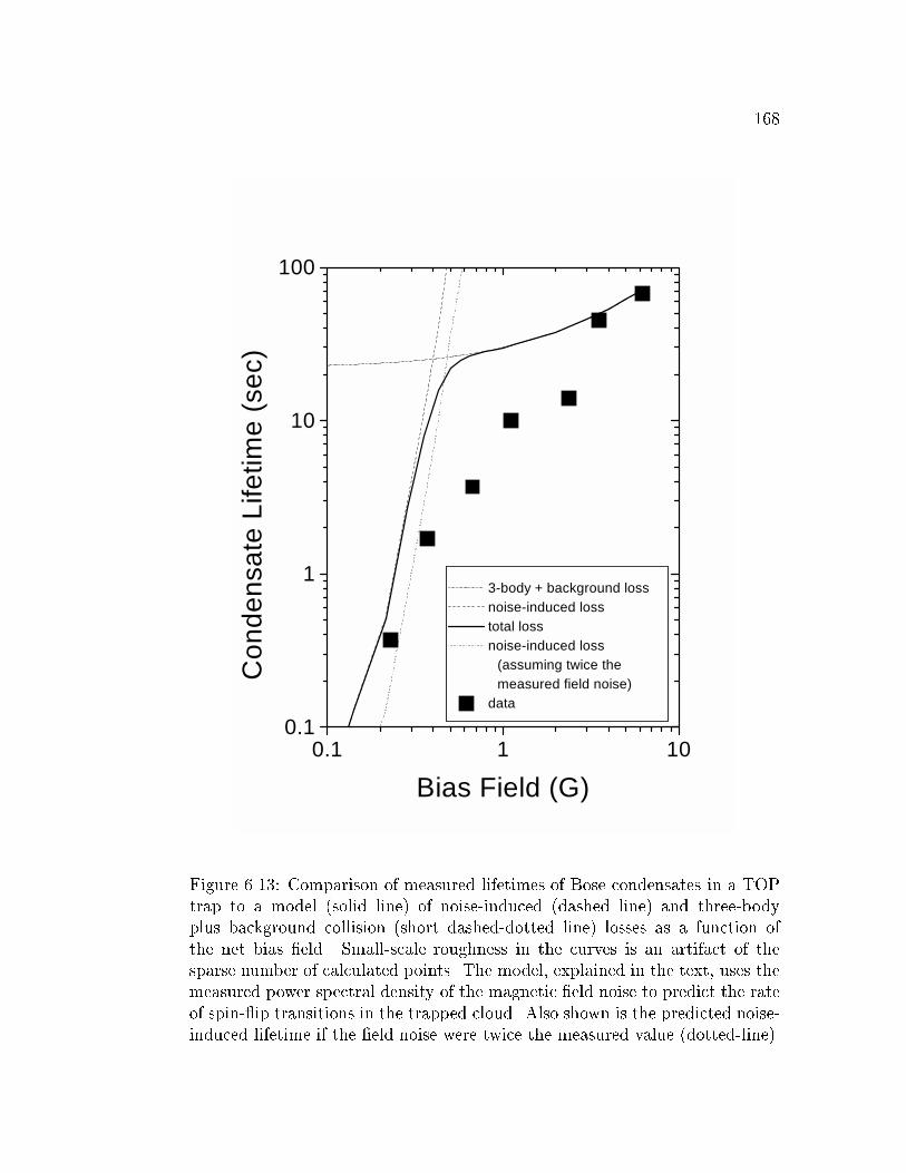
168
0.1 1 100.1
1
10
100
3-body + background loss noise-induced loss total loss noise-induced loss
(assuming twice the measured field noise)
data
Con
dens
ate
Life
time
(sec
)
Bias Field (G)
Figure 6.13: Comparison of measured lifetimes of Bose condensates in a TOP
trap to a model (solid line) of noise-induced (dashed line) and three-body
plus background collision (short dashed-dotted line) losses as a function of
the net bias �eld. Small-scale roughness in the curves is an artifact of the
sparse number of calculated points. The model, explained in the text, uses the
measured power spectral density of the magnetic �eld noise to predict the rate
of spin- ip transitions in the trapped cloud. Also shown is the predicted noise-
induced lifetime if the �eld noise were twice the measured value (dotted-line).

169
6.6 E�ects of Bias Field Rotation Frequency
As was mentioned at the end of Section 6.2.1, the original TOP trap
easily satis�ed the limiting conditions 6.1, and long trap lifetimes were observed
[21]. To our knowledge, no one has ever performed experiments to determine
at which rotation frequencies !T, relative to trap oscillation frequencies and
Larmor frequency, the TOP trap no longer holds atoms. In this section we
study the lifetime of atoms in the TOP trap as a function of !T to experimen-
tally quantify the breakdown of the time-averaging and adiabaticity conditions
6.1 in the TOP trap. Breaching the adiabaticity condition 6.1b is especially
interesting as it may play a role in increasing loss in the TOP at small bias
�elds. In our study of lifetime versus magnetic �eld, !T was held �xed while
the bias �eld, and hence the Larmor frequency, was reduced.
The experimental method is much the same as for studying the life-
time in the TOP at di�erent bias �elds. We begin each experimental cycle in
a TOP trap of 1.8 kHz bias rotation frequency. After evaporatively cooling
the cloud until only a pure condensate remains we then adiabatically ramp
the trap �elds to the desired bias �eld and trap frequencies. We then change
the TOP rotation frequency in . 0:5 ms, simultaneously adjusting the relative
gain and phase of the TOP channels. The gain and phase shift adjustments
compensate for the frequency-dependent gain and phase shifts of the TOP cir-
cuit and preserve the eccentricity and bias �eld for TOP frequencies other than
1.8 kHz. Technical limitations unfortunately prevent us from making the rota-
tion frequency either less than the trap frequencies or greater than the Larmor
frequency [191]. The atoms remain in the TOP trap for a variable dwell time,
after which the TOP rotation frequency is returned to 1.8 kHz with the ap-

170
propriate channel gains and phases. Once returned to the 1.8 kHz trap, the
atoms are probed with absorption imaging to count the remaining atoms. This
method of in situ frequency adjustment allows us to create and probe clouds
in a standard TOP trap whose critical timing is always the same, regardless of
the rotation frequency we wish to study.
In a �rst experiment, we study the lifetimes of condensates of �
7:5�108 atoms in a trap with frequencies fx = 36 Hz and fz = 87 Hz (Fig.6.14,
solid squares). The bias �eld is 0.59 Gauss (413 kHz Larmor frequency). At
1.8 kHz the lifetime is 1.9 sec, consistent with previously measured low-�eld
lifetimes. Over the decade of TOP frequencies up to 18 kHz the lifetime de-
creases only 15%, but at 27 kHz plummets to 0.2 sec. Decreasing the TOP
rotation frequency from 1.8 kHz, the lifetime steadily decreases to 0.4 sec at
0.2 kHz.
In our second experiment we attempt to improve the sensitivity of
the lifetimes to losses at extreme TOP frequencies by reducing the three-body
recombination limit to the lifetime. We decrease the initial condensate density
both by using only � 1 � 104 atoms and lowering the trap frequencies to
fx = 23 Hz and fz = 43 Hz [192]. The bias �eld is 0.65 Gauss (455 kHz
Larmor frequency). The data are shown in Figure 6.14 (solid circles). The
lifetime at 1.8 kHz is improved to 9 sec and remains approximately constant
with frequency, up to 27 kHz. Decreasing the TOP frequency from 1.8 to 0.35
kHz decreases the lifetime by a factor of 2, in qualitative agreement with the
0.59 Gauss data.
For our �nal experiment we focused on losses at high TOP frequencies
by reducing the Larmor frequency (Figure 6.14, empty triangles). We use an
intermediate number of atoms (� 2�105) and low trap frequencies (fx = 23 Hz

171
and fz = 48 Hz) to reduce three-body collisions. Working in a trap with bias
�eld of 0.36 Gauss the Larmor frequency, 250 kHz, is just 9.3 times larger than
the 27 kHz maximum TOP frequency. Increasing the TOP frequency from 1.8
to 27 kHz decreased the TOP lifetime by almost a factor of �ve.
Interpreting these data is di�cult for several reasons. Let us begin
with an examination of the data at high rotation frequencies. We point out
that in a trap with 0.59 Gauss bias �eld the lifetime at 27 kHz rotation fre-
quency is a factor of 10 smaller than at 18 kHz. In contrast, even though the
Larmor frequency is virtually identical, lifetimes taken in the 0.65 Gauss trap
for 27 and 18 kHz rotation frequencies are the same, within the experimental
error bars. Such inconsistency may be due, in large measure, to the technical
di�cult of consistently creating a TOP trap with 27 kHz rotation frequency.
We experience even greater problems in the data at low frequencies: in addition
to the challenge of making a 200 Hz rotation frequency in our TOP circuit,
the short lifetime measured at 200 Hz could be interpreted as the result of
noise at 60 Hz or its harmonics. The data at 0.65 Gauss, excluding the 27 kHz
data point, cover a wide range of rotation frequencies that are also far from
the ambiguous regions of operation mentioned above. The best conclusion we
are able to draw from these data is that if !T is at least 25 times smaller than
the Larmor frequency and at least 8 times larger than the axial trap frequency,
then the TOP trap lifetime is not decreased due to violations of the basic TOP
trap conditions 6.1b and 6.1a. Although the conclusion is less de�nitive than
initially intended, it nonetheless reveals that the reduction in trap lifetimes at
low bias �elds cannot be due to loss of adiabaticity in the TOP trap. In the
bias �eld data (Fig. 6.10), the Larmor frequency is at least 90 times larger
than the TOP rotation frequency.

172
0.1 1 100.1
1
10
0.65 G 0.59 G 0.36 G
Con
dens
ate
Life
time
(sec
)
TOP Rotation Frequency (kHz)
Figure 6.14: Lifetimes of Bose condensates in a TOP trap as a function of the
frequency of the rotating bias �eld, for three di�erent values of the bias �eld.
The solid circles are measured in a trap of 0.65 Gauss bias �eld, fx = 23 Hz
and fz = 43 Hz. The solid squares are measured in a trap with 0.59 Gauss bias
�eld, fx = 36 Hz and fz = 87 Hz. The empty triangles are measured in a trap
with 0.36 Gauss bias �eld, fx = 28 Hz and fz = 48 Hz. The Larmor frequency
is 700 kHz/Gauss.

173
6.7 Summary and Conclusions
In this chapter we have explored the properties of the TOP magnetic
trap both theoretically and experimentally. We rederived the time-averaged
orbiting potential including the e�ects of gravity and found corrections to the
spring constants that depend on the strength of the quadrupole gradient. Tun-
ing the gradient adjusts the trap aspect ratio fromp8 to less than 1. Simple
control over the aspect ratio should permit study of the resonant response of
the collective excitations of Bose condensates to trap symmetries [193]. We
also precisely calculated the anharmonicity of the TOP and found that, for
reasonable experimental conditions, the anharmonic terms introduce less than
a 1% fractional shift in the axial and radial frequencies. Low anharmonici-
ties should improve at least two classes of experiment. First, elimination of
anharmonic dephasing will allow unambiguous identi�cation of the damping
mechanisms in condensate collective excitations [194]. Second, reducing sys-
tematic uncertainties in frequency will enable precision measurement of the
condensate excitation frequencies beyond the 1% level, o�ering a �rst glimpse
at many-body physics in the condensate [195].
We have studied TOP trap lifetimes operating the trap under various
extreme conditions. We now understand several of the loss mechanisms that
plague magnetic traps operating with very small bias �elds. Above 1 Gauss,
we observe a loss process in which atoms are lost from the observable cloud but
remain trapped at higher energy, and subsequently collide with the observable
cloud leading to an enhanced loss. We suppress the loss with an rf magnetic
�eld (rf shield). Below 1 Gauss, the trap lifetime is strongly reduced and the
mechanism is not as well understood. We have eliminated processes due to the

174
�nite depth of the TOP trap and cloud density. A possible candidate is broad-
band magnetic �eld noise that weakly drives atoms into untrapped atomic
states. The mechanism is rather generic and may be the primary technical
limitation to low magnetic �eld lifetimes in all magnetic traps. Reducing mag-
netic �eld noise could allow evaporative cooling in atomic Cs to reach BEC. In
other studies we attempted to quantify the TOP criteria 6.1. We can conclude
that there is no change in TOP trap lifetime when the rotation frequency is at
least 25 times smaller than the Larmor frequency, and at least 8 times larger
than the axial trap oscillation frequency. Unfortunately, technical problems
impair our ability to draw conclusions about the trap lifetimes at rotation fre-
quencies closer to the Larmor frequency and trap frequencies. This �nding
eliminates loss-of-adiabaticity in the TOP as a mechanism for the losses from
low-bias �eld traps reported here.
The TOP and IP magnetic traps o�er a multitude of options for
experiments with trapped atoms and BEC. With the results of the present
work and other insights we have made over the past several years we can now
place the TOP trap in its context as a tool for the atomic physicist. Table 6.2
summarizes some of the advantages and disadvantages of the TOP magnetic
trap. The TOP is clearly not always the best magnetic trap. For the largest
�eld gradients and tightest con�nement an IP trap (for example, the cloverleaf
design [121]) is still better. IP traps can also achieve much larger di�erences in
axial and radial frequencies in cylindrically symmetric traps. Large bias �elds
(> 100 G) rotating at several kHz are di�cult to generate, given limitations on
power dissipation. Thus, exploiting most of the Feshbach resonances predicted
in alkali atoms is only feasible in IP traps [196, 197]. Even a modest TOP
bias �eld is di�cult to generate if a steel vacuum system is used, due to eddy

175
currents [198]. Both limits to the bias �eld limit the depth of the TOP, and
probably prohibits loading atom samples that are not cooled below the Doppler
Temperature. Finally, the time-dependent nature of the magnetic �elds can
complicate precision metrology in a TOP at the kHz level, such as measurement
of atomic hyper�ne transitions [199].
On the other hand, the TOP trap is very simple and contains a num-
ber of features that are nearly as good as, if not superior to, the IP traps. The
TOP can cover a wide range of frequencies (almost a factor of 80, from a few
Hz to 300 Hz axially) and bias �elds (a factor of 250, from 0.2 to 50 Gauss).
The TOP design is fairly economical: It requires only six coils, two of which
are the anti-Helmholtz coils that are already part of experiments using MOT's.
As a result, loading the atoms into the TOP trap from the MOT is relatively
simple because the centers of MOT and TOP are quasi-aligned. The rotating
bias �eld is a natural quantization axis that can be used over all 360� of the
rotation plane. The time-dependence of the bias, while a hinderance to some
precision measurements, can be a feature as well. Adjusting the frequency
and amplitude of the rotating bias is a way to carefully control the amount of
relative sag between states whose magnetic moments are identical [199, 163].
The rotation is also a natural method of angular averaging { an e�ect that can
substantially reduce systematic errors in measurements of beta decay [200]. In
terms of evaporative cooling, the TOP trap is assured of having at least 2-d
evaporation, whereas gravitational sag can sometimes limit IP traps to 1-d. In
fact, the quadrupole zero alone can perform evaporative cooling without any
rf required [201]. We believe that these positives and the features discussed in
the present work will continue to make the TOP magnetic trap an attractive
choice for a number of experiments.

176
Positive Negative
1. simple, compact 6 coil design 1. gradients and trap frequencies
smaller than Cloverleaf IP traps
2. simple, analytical potential 2. low-trap depths and limited maxi-
mum cloud sizes
3. tunable aspect ratio: < 1$p8 3. large bias �elds > 100 G are di�-
cult
4. low anharmonicities for most trap
symmetries
4. asymmetry abovep8 not possible
for high frequencies
5. wide frequency range 5. synchronization electronics, trans-
formers needed
6. intrinsic bias �eld/quantization
axis with 2� orientation angles
6. rotating �eld causes eddy-current
heating of stainless-steel cells and
limits size of bias �eld [198]
7. variable drive symmetries for creat-
ing excitations in trapped clouds
7. lifetime below 1 G is short
8. near-cylindrical symmetry easy 8. di�cult to achieve 3-D evaporation
9. center of TOP is very near the cen-
ter of MOT due to quadrupole �eld
9. shaving loss from quadrupole zero
10. tunable sag in trap for di�erent hy-
per�ne states [199]
10. time-dependent �eld complicates
precision metrology
11. low-bias �eld traps easy to make
12. cylindrically symmetric TOP al-
ways has 2-D RF evaporative cool-
ing
13. stray DC magnetic �elds only shift
trap center and don't alter trap
shape
14. no large uctuation in net bias �eld
15. built in 2-D evaporation from
quadrupole zero [201]
16. rotating bias averages over all an-
gles
Table 6.2: Positive and Negative Features of the TOP Magnetic Trap

Bibliography
[1] This paper �rst appeared in J. Opt. Soc. Am. B 11, 1332 (1994).
[2] This paper �rst appeared in Phys. Rev. A, 50 R3597 (1994).
[3] This paper �rst appeared in Phys. Rev. Lett., 74 3352 (1995).
[4] This paper �rst appeared in Science 269, 133 (1995).
[5] F. Dalfovo and S. Stringari, Phys. Rev. A 53, 2477 (1996).
[6] D. S. Jin et al., Czech. J. Phys. 46, 3070 (1996), Suppl. S6.
[7] M. J. Holland, D. S. Jin, M. L. Chiofalo, and J. Cooper, Phys. Rev. Lett.
78, 3801 (1997).
[8] D. S. Jin et al., Phys. Rev. Lett. 77, 420 (1996).
[9] M. Edwards et al., Phys. Rev. Lett. 77, 1671 (1996).
[10] P. A. Ruprecht, M. Edwards, K. Burnett, and C. W. Clark, Phys. Rev.
A 54, 4178 (1996).
[11] B. D. Esry and C. H. Greene, Private Communication, 1996.
[12] S. Stringari, Phys. Rev. Lett. 77, 2360 (1996).
[13] J. R. Ensher et al., Phys. Rev. Lett. 77, 4984 (1996).
[14] S. Grossmann and M. Holthaus, Phys. Lett. A 208, 188 (1995).
[15] W. Ketterle and N. J. van Druten, Phys. Rev. A 54, 656 (1996).
[16] W. H. Keesom and K. Clusius, Proc. Roy. Acad. Amsterdam 35, 307
(1932).
[17] W. H. Keesom and A. P. Keesom, Proc. Roy. Acad. Amsterdam 35, 736
(1932).

178
[18] A. Minguzzi, S. Conti, and M. P. Tosi, Jour. Phys. - Cond. Matt. 9, L33
(1997).
[19] W. Petrich, M. H. Anderson, J. R. Ensher, and E. A. Cornell, J. Opt.
Soc. Am. B 11, 1332 (1994).
[20] M. H. Anderson, W. Petrich, J. R. Ensher, and E. A. Cornell, Phys. Rev.
Lett. 50, R3597 (1994).
[21] W. Petrich, M. H. Anderson, J. R. Ensher, and E. A. Cornell, Phys. Rev.
Lett. 74, 3352 (1995).
[22] M. H. Anderson et al., Science 269, 198 (1995).
[23] A. Einstein, Sitzungsber. Kgl. Preuss. Akad. Wiss. 1924, 261 (1924).
[24] S. Bose, Z. Phys. 26, 178 (1924).
[25] K. Huang, Statistical Mechanics (John Wiley and Sons, New York, 1987).
[26] M. Bijlsma and H. T. C. Stoof, Phys. Rev. A 54, 5085 (1996).
[27] N. J. van Druten and W. Ketterle, Phys. Rev. Lett. 79, 549 (1997).
[28] Actually, the notion that super uidity was a manifestation of Bose-
Einstein Condensation was seen as highly controversial in the early theory
of liquid Helium. Landau rejected the idea in favor of quantum hydrody-
namics. See the Ref. [37] for more discussion.
[29] G. E. Brown, in Bose-Einstein Condensation, edited by A. Gri�n, D. W.
Snoke, and S. Stringari (Cambridge University Press, Cambridge, 1995),
Chap. 18, pp. 438{451.
[30] J. Ranninger, in Bose-Einstein Condensation, edited by A. Gri�n, D. W.
Snoke, and S. Stringari (Cambridge University Press, Cambridge, 1995),
Chap. 16, pp. 393{417.
[31] F. Iachello, in Bose-Einstein Condensation, edited by A. Gri�n, D. W.
Snoke, and S. Stringari (Cambridge University Press, Cambridge, 1995),
Chap. 17, pp. 418{437.
[32] J. L. Lin and J. P. Wolfe, Phys. Rev. Lett 71, 1222 (1993).
[33] A. Mysyrowicz, D. Hulin, and A. Antonetti, Phys. Rev. Lett. 43, 1123
(1979).
[34] E. Fortin, S. Fafard, and A. Mysyrowicz, Phys. Rev. Lett. 70, 3951
(1993).

179
[35] A. Einstein, Sitzungsber. Kgl. Preuss. Akad. Wiss. 1925, 3 (1925).
[36] English translation of Einstein's quotes and historical interpretation are
from A. Pais, Subtle is the Lord..., (Oxford University Press, Oxford,
1982).
[37] K. Gavroglu, Fritz London (Cambridge University Press, New York,
1995).
[38] F. London, Nature 141, 643 (1938).
[39] L. Tisza, Nature 141, 913 (1938).
[40] L. D. Landau, J. Phys. Moscow 5, 71 (1941).
[41] R. P. Feynman, in Progress in Low Temperature Physics, edited by C. J.
Gorter (North-Holland, Amsterdam, 1955), Vol. I, p. 17.
[42] L. P. Pitaevski, Sov. Phys. JETP 12, 155 (1961).
[43] P. Sokol, in Bose-Einstein Condensation, edited by A. Gri�n, D. W.
Snoke, and S. Stringari (Cambridge University Press, Cambridge, 1995),
Chap. 4, pp. 51{85.
[44] D. M. Ceperley, Rev. Mod. Phys. 67, 279 (1995).
[45] C. E. Hecht, Physica 25, 1159 (1959).
[46] W. C. Stwalley and L. H. Nosanow, Phys. Rev. Lett. 36, 910 (1976).
[47] I. F. Silvera and J. T. M. Walraven, Phys. Rev. Lett. 44, 164 (1980).
[48] W. N. Hardy, M. Morrow, R. Jochemsen, and A. J. Berlinsky, Physica
109, 1964 (1982).
[49] H. F. Hess et al., Phys. Rev. Lett. 51, 483 (1983).
[50] B. R. Johnson et al., Phys. Rev. Lett. 52, 1508 (1984).
[51] D. A. Bell et al., Phys. Rev. B 34, 7670 (1986).
[52] R. Sprik, J. T. M. Walraven, and I. F. Silvera, Phys. Rev. B 32, 5668
(1985).
[53] H. F. Hess, Phys. Rev. B. 34, 3476 (1986).
[54] Proceedings of the International School of Physics `Enrico Fermi', Course
CXVIII, Laser Manipulation of Atoms and Ions, edited by E. Arimondo,
W. D. Phillips, and F. Strumia (North Holland, Amsterdam, 1992).

180
[55] S. Chu, Rev. Mod. Phys. 70, 685 (1998).
[56] C. N. Cohen-Tannoudji, Rev. Mod. Phys. 70, 707 (1998).
[57] W. D. Phillips, Rev. Mod. Phys. 70, 721 (1998).
[58] D. J. Wineland and H. Dehmelt, Bull, Am. Phys. Soc. 20, 637 (1975).
[59] T. W. H�ansch and A. L. Schawlow, Opt. Commun. 13, 68 (1975).
[60] V. Letokhov, Pis'ma Zh. Eksp. Teor. Fiz. 7, 348 (1968).
[61] J. E. Bjorkholm, R. E. Freeman, A. Ashkin, and D. Pearson, Phys. Rev.
Lett. 41, 1361 (1978).
[62] W. Neuhauser, M. Hohenstatt, P. Toschek, and H. Dehmelt, Phys. Rev.
Lett. 41, 233 (1978).
[63] D. J. Wineland, R. E. Drullinger, and F. L. Walls, Phys. Rev. Lett. 40,
1639 (1978).
[64] S. V. Andreev, V. I. Balykin, V. S. Letokhov, and V. G. Minogin, Pis'ma
Zh. Eksp. Teor. Fiz. 34, 463 (1981), [JETP Lett., 34, 442 (1981)].
[65] J. Prodan et al., Phys. Rev. Lett. 54, 992 (1985).
[66] W. Ertmer, A. Migdall, J. L. Hall, and M. Zhu, Phys. Rev. Lett. 54, 996
(1985).
[67] S. Chu et al., Phys. Rev. Lett. 55, 48 (1985).
[68] W. D. Phillips, J. V. Prodan, and H. J. Metcalf, J. Opt. Soc. Am. B 2,
1751 (1985).
[69] A. Aspect et al., Phys. Rev. Lett. 57, 1688 (1986).
[70] P. J. Martin et al., Phys. Rev. A 36, 2495 (1987).
[71] S. Chu, J. E. Bjorkholm, A. Ashkin, and A. Cable, Phys. Rev. Lett. 57,
314 (1986).
[72] E. L. Raab et al., Phys. Rev. Lett. 59, 2631 (1987).
[73] P. D. Lett et al., Phys. Rev. Lett. 61, 169 (1988).
[74] J. Dalibard et al., in Proceedings of the 11th International Conference
on Atomic Physics, edited by S. Haroche, J. C. Gay, and G. Grynberg
(World Scienti�c, Singapore, 1989), pp. 199{214.
181
[75] S. Chu, D. S. Weiss, Y. Shevy, and P. J. Ungar, in Proceedings of the 11th
International Conference on Atomic Physics, edited by S. Haroche, J. C.
Gay, and G. Grynberg (World Scienti�c, Singapore, 1989), pp. 636{638.
[76] J. Dalibard and C. Cohen-Tannoudji, J. Opt. Soc. Am. B 6, 2023 (1989).
[77] T. Walker, D. Sesko, and C. Wieman, Phys. Rev. Lett. 64, 408 (1990).
[78] N. Davidson, H.-J. Lee, M. Kasevich, and S. Chu, Phys. Rev. Lett. 72,
3158 (1994).
[79] J. Lawall et al., Phys. Rev. Lett. 75, 4194 (1995).
[80] W. Ketterle et al., Phys. Rev. Lett. 70, 2253 (1993).
[81] Although see H. J. Lee and S. Chu, Phys. Rev. A. 57, 2905 (1998) for
recent progress, and a preprint by H. Katori, T. Ito, Y. Isoya and M.
Kuwata-Gonokami.
[82] D. E. Pritchard, Phys. Rev. Lett. 51, 1336 (1983).
[83] A. L. Migdall et al., Phys. Rev. Lett. 54, 2596 (1985).
[84] V. S. Bagnato et al., Phys. Rev. Lett. 58, 2194 (1987).
[85] R. V. E. Lovelace, C. Mehanian, T. J. Tommila, and D. M. Lee, Nature
318, 30 (1985).
[86] J. M. Doyle et al., Phys. Rev. Lett. 67, 603 (1991).
[87] J. M. Doyle, Ph.D. thesis, Massachusetts Institute of Technology, 1991.
[88] O. J. Luitin et al., Phys. Rev. Lett. 70, 544 (1993).
[89] C. Monroe, W. Swann, H. Robinson, and C. Wieman, Phys. Rev. Lett.
65, 1571 (1990).
[90] C. Monroe, E. Cornell, and C. Wieman, in Proceedings of the
International School of Physics `Enrico Fermi', Course CXVIII, Laser
Manipulation of Atoms and Ions, edited by E. Arimondo, W. D. Phillips,
and F. Strumia (North Holland, Amsterdam, 1992), pp. 361{377.
[91] E. A. Cornell, C. Monroe, and C. E. Wieman, Phys. Rev. Lett. 67, 2439
(1991).
[92] C. R. Monroe et al., Phys. Rev. Lett. 70, 414 (1993).
[93] C. J. Myatt et al., Opt. Lett. 21, 290 (1996).

182
[94] N. R. Newbury, C. J. Myatt, and C. E. Wieman, Phys. Rev. A 51, R2680
(1995).
[95] J. D. Gillaspy, I. F. Silvera, and J. S. Brooks, Phys. Rev. B 40, 210
(1989).
[96] Y. Kagan, I. A. Vartanyants, and G. V. Shlyapnikov, Sov. Phys. JETP
54, 590 (1981).
[97] Y. Kagan, G. V. Shlyapnikov, and I. A. Vartanyants, Phys. Lett. 101A,
27 (1984).
[98] A. Lagendijk, I. F. Silvera, and B. J. Verhaar, Phys. Rev. B 33, 626
(1986).
[99] D. E. Pritchard, in Electronic and Atomic Collisions, edited by D. C.
Lorents, W. E. Meyerhof, and J. R. Peterson (North Holland, Amster-
dam, 1986), pp. 593{604.
[100] M. Prentiss et al., Opt. Lett. 13, 452 (1988).
[101] P. L. Gould et al., Phys. Rev. Lett. 60, 788 (1988).
[102] D. Sesko et al., Phys. Rev. Lett. 63, 961 (1989).
[103] K. Gibble and S. Chu, Phys. Rev. Lett. 70, 1771 (1993).
[104] K. B. Davis et al., Phys. Rev. Lett. 74, 5202 (1995).
[105] H. R. Thorsheim, J. Weiner, and P. S. Julienne, Phys. Rev. Lett. 58,
2420 (1987).
[106] J. D. Miller, R. A. Cline, and D. J. Heinzen, Phys. Rev. Lett. 71, 2204
(1993).
[107] P. D. Lett et al., Phys. Rev. Lett. 71, 2200 (1993).
[108] J. R. Gardner et al., Phys. Rev. Lett. 74, 3764 (1995).
[109] W. I. McAlexander et al., Phys. Rev. A 51, R871 (1995).
[110] E. R. I. Abraham, W. I. McAlexander, C. A. Sackett, and R. G. Hulet,
Phys. Rev. Lett. 74, 1315 (1995).
[111] K. Gibble, S. Chang, and R. Legere, Phys. Rev. Lett. 75, 2666 (1995).
[112] C. G. Townsend et al., Phys. Rev. A 52, 1423 (1995).

183
[113] W. Ketterle, Private Communication, 1995.
[114] J. J. Tollett, C. C. Bradley, C. A. Sackett, and R. G. Hulet, Phys. Rev.
A 51, R22 (1995).
[115] D. Pritchard et al., in Proceedings of the 11th International Conference
on Atomic Physics, edited by S. Haroche, J. C. Gay, and G. Grynberg
(World Scienti�c, Singapore, 1989), pp. 619{621.
[116] A. G. Martin et al., Phys. Rev. Lett. 61, 2431 (1988).
[117] C. S. Adams et al., Phys. Rev. Lett. 74, 3577 (1995).
[118] R. G. Hulet, Bull. Am. Phys. Soc. 40, 1267 (1995).
[119] K. B. Davis et al., Phys. Rev. Lett. 75, 3969 (1995).
[120] C. C. Bradley, C. A. Sackett, J. J. Tollett, and R. G. Hulet, Phys. Rev.
Lett. 75, 1687 (1995), ibid. 79, 1170 (1997).
[121] M.-O. Mewes et al., Phys. Rev. Lett. 77, 416 (1996).
[122] C. J. Myatt et al., Phys. Rev. Lett. 78, 586 (1997).
[123] This chapter is an expanded version of material that appeared in Ref.
[6].
[124] L. P. Pitaevski, Sov. Phys. JETP 13, 451 (1961).
[125] E. P. Gross, Nuovo Cimento 20, 454 (1961).
[126] E. P. Gross, J. Math. Phys. 4, 195 (1963).
[127] The system is dilute if the interparticle spacing is much larger than the
two-body scattering length a describing binary collisions between bosons.
In other words, na3 � 1 where n is the density. By this standard, con-
densates of 87Rb [22] are indeed dilute: with densities of up to � 1013
atoms/cm3 and a � 6:0 nm the product na3 � 10�6.
[128] In the Gross-Pitaevskii equation, the ratio of interaction strength to the
harmonic oscillator energy scales as na=�r, where n is the density of the
condensate wavefunction. For the current experiments, the interactions
are weak enough that the density pro�le is still approximately Gaussian,
for which n � N�3=2r . In contrast, in the Thomas-Fermi limit the inter-
actions are so strong that the density pro�le is a paraboloid for which
n � N2=5�6=5r .

184
[129] V. V. Goldman, I. F. Silvera, and A. J. Leggett, Phys. Rev. B 24, 2870
(1981).
[130] G. Baym and C. J. Pethick, Phys. Rev. Lett. 76, 6 (1996).
[131] H. M. J. M. Boesten, C. C. Tsai, D. J. Heinzen, and B. J. Verhaar,
Private Communication, 1996.
[132] H. F. Hess et al., Phys. Rev. Lett. 59, 672 (1987).
[133] The release of the atoms for ballistic expansion is initiated by a sudden
increase in the transverse bias �eld, which quenches the con�ning forces
on a time-scale fast compared to any cloud dynamics. Interactions and
residual kinetic energy cause the cloud to y apart. The error in the �nal
velocity determination due to residual magnetic �elds is less than 2%.
[134] A. L. Fetter, Czech. J. Phys. 46, 547 (1996), Suppl. S1.
[135] K. Singh and D. Rokhsar, Private Communication, 1996.
[136] This chapter is an expanded version of material that appeared in Ref.
[8].
[137] The remaining noncondensate atoms represent less than 20% of the sam-
ple. We �nd good agreement between the calculated and measured BEC
transition temperatures; this data will be presented in a future paper.
[138] A. L. Fetter and J. D. Walecka, Quantum Theory of Many-Particle
Systems (McGraw-Hill, New York, 1971).
[139] A connection between the phase of the condensate perturbation and the
ultimate width of the expanded cloud may be obtained by numerical
integration of the non-linear Schr�odinger equation. See for example P. A.
Ruprecht, M. J. Holland, K. Burnett, and M. Edwards, Phys. Rev. A 51,
4704 (1995); M. Holland and J. Cooper, Phys. Rev. A 53, 1954 (1996).
[140] N. N. Bogoliubov, J. Phys. Moscow 11, 23 (1947).
[141] D. S. Jin et al., Phys. Rev. Lett. 78, 764 (1997).
[142] C. C. Bradley, C. A. Sackett, and R. G. Hulet, Phys. Rev. Lett. 78, 985
(1997).
[143] M.-O. Mewes et al., Phys. Rev. Lett. 77, 988 (1996).
[144] This chapter is an expanded version of material that appeared in Ref.
[13].

185
[145] Some smoothing is performed in the wings of the distribution, where
signal-to-noise is poor, using the same set of assumptions we use for
thermometry.
[146] As the excluded central region is enlarged, systematic bias in the inferred
temperature vanishes, but so does signal-to-noise. We found it necessary
to �t to a region which unfortunately samples the outer edge of the
degenerate portion of the cloud. From numerical studies of the ideal Bose-
Einstein distribution, we derive and apply a modest (< 10%) correction
to the measured temperature. The feature we see in the cloud energy
occurs regardless of whether we include this correction.
[147] S. R. de Groot, G. J. Hooyman, and C. A. ten Seldam, Proc. R. Soc. A
203, 266 (1950).
[148] F. Dalfovo, S. Giorgini, L. Pitaevskii, and S. Stringari, Czech. J. Phys.
46, 545 (1996), Suppl. S1.
[149] M. Bijlsma and H. T. C. Stoof, Czech. J. Phys. 46, 553 (1996), Suppl.
S1.
[150] H. J. Davies and C. S. Adams, Phys. Rev. A 55, R2527 (1997).
[151] S. Giorgini, L. P. Pitaevskii, and S. Stringari, Phys. Rev. Lett. 78, 3987
(1997).
[152] C. J. Myatt, Ph.D. thesis, University of Colorado, 1997.
[153] From Eq.(1.5), the collection rate of a vapor cell MOT scales as R �V 2=3v4c . The MOT volume V = L3, where the volume is assumed to
be a cube with side length L equal to the MOT beam diameter. The
capture velocity vc is proportional to the deceleration from spontaneously
scattered photons and the distance over which that force acts. Thus,
vc � IL2, where I is the laser intensity, and the collection rate R � I2L4.
[154] We use a 5 cm high breadboard that is more than rigid enough. The
excess height of the breadboard reduces the optical access below the cells
because our standard height for laser beams is only 15.2 cm. The entire
vacuum system may be elevated even higher than the beam heights, but
that introduces other problems: the beams are raised closer to eye levels
and longer mounts are required, making the entire system more prone to
vibrations.
[155] K. B. MacAdam, A. Steinbach, and C. Wieman, Am. J. Phys. 60, 1098
(1992).

186
[156] F. E. Terman, Radio Engineers' Handbook, textbook ed. (McGraw-Hill,
New York, 1943), pp. 53{64.
[157] C. R. Monroe, Ph.D. thesis, University of Colorado, 1992.
[158] D. Ho�mann, P. Feng, and T. Walker, Measurements of Rb trap-loss
collision spectra, 1994.
[159] Z. T. Lu et al., Phys. Rev. Lett. 77, 3331 (1996).
[160] E. Majorana, Nuovo Cimento 8, 107 (1931).
[161] J. Dalibard, Private Communication, 1998.
[162] T. Esslinger, I. Bloch, and T. W. H�ansch, Phys. Rev. A 58, R2664 (1998).
[163] D. S. Hall et al., Phys. Rev. Lett. 81, 1539 (1998).
[164] D. J. Han, R. H. Wynar, P. Courteille, and D. J. Heinzen, Phys. Rev. A
57, R4114 (1998).
[165] B. P. Anderson and M. A. Kasevich, Bull. Am. Phys. Soc. 43, 1251
(1998).
[166] A. Wilson, Private Communication, 1998.
[167] L. Deng et al., Bull. Am. Phys. Soc. 43, 1379 (1998).
[168] M. Arndt et al., Phys. Rev. Lett. 79, 625 (1997).
[169] J. Arlt et al., J. Phys. B 31, L321 (1998).
[170] E. Arimondo, Private Communication, 1998.
[171] T. Bergeman, G. Erez, and H. Metcalf, Phys. Rev. A 35, 1535 (1987).
[172] M. R. Matthews et al., Phys. Rev. Lett. 81, 243 (1998).
[173] V. E. Shapiro, Phys. Rev. A 54, R1018 (1996).
[174] A. B. Kuklov et al., Phys. Rev. A 55, 488 (1997).
[175] J. D. Luca, R. Napolitano, and V. S. Bagnato, Phys. Rev. A 55, R1597
(1997).
[176] V. I. Yukalov, Phys. Rev. A 56, 5004 (1997).
[177] V. Minogin, J. A. Richmond, and G. I. Opat, Phys. Rev. A 58, 3138
(1998).

187
[178] J. Dalibard, Lectures at the 1998 Enrico Fermi Summer School on BEC
in Varenna, Italy.
[179] L. D. Landau and E. M. Lifshitz, Mechanics, 3rd ed. (Pergamon Press,
Oxford, 1973).
[180] It should be possible to use large radial symmetry breaking in a rotating
magnetic potential to impart angular momentum to cold atom clouds.
[181] We minimize phase uncertainty in the measured frequencies by �tting
complete oscillation periods many periods apart. Systematic uncertain-
ties due to anharmonic frequency shifts are below 0:1%.
[182] The argument in this paragraph is due to C. Monroe and E. Cornell. The
results have been numerically validated by B. Verhaar's group.
[183] J. S�oding et al., Phys. Rev. Lett. 80, 1869 (1998).
[184] E. A. Burt et al., Phys. Rev. Lett. 79, 337 (1997).
[185] M. E. Gehm, K. M. O'Hara, T. A. Savard, and J. E. Thomas, Phys. Rev.
A 58, 3914 (1998).
[186] The exponential decay curve suggests that the loss mechanism is more
complicated than three three-body dominated loss, which should show a
non-exponential loss of atoms with time.
[187] Our noise detection method provides a genuine measure of the noise
on the TOP coils and an estimate of the noise near the atoms that is
better than a factor of two. Noise power registered on the pick-up coil
directly re ects noise on the TOP coil because the pick-up coil is wrapped
immediately next to one of the TOP coils. The absolute noise voltage
registered on the rf spectrum analyzer is calibrated with a digital FFT.
The uncertainty in the measured voltage, determined by statistical noise
in the power spectrum, is less than 3 dB. The resonance frequency of the
pick-up coil does not in uence the measured voltage since the resonance
occurs at a much higher frequency than what we measure. We calculate
the magnetic �eld noise at the location of the atoms from an estimate of
the distance between the trapped atoms and the TOP coil.
[188] The details of this approach are discussed in Ref. [185], in the context
of noise-induced heating in traps. We similarly reason that the averaging
time T is short compared to the time scale over which the level popula-
tions change, but is long compared to the correlation time of the magnetic
�eld uctuations.
188
[189] We assume that the loss rate is slow enough that (i) once an atom has
made a transition to the m = 0 state it is lost from the trap before it can
return to the m = �1 state; and (ii) the time-averaged magnetic �eld
determines the Zeeman splitting at a point ~r in the potential. The roll-
o� in the power spectral density at high frequencies implies that atoms
further from the trap center, which sample larger magnetic �elds, are less
likely to be lost from the trap.
[190] The three-body recombination rate is calculated assuming a per atom
rate that is constant with magnetic �eld, using the initially measured
condensate central density. Thus, the rate is an upper limit to the rate
of loss we expect from recombination events. The background collision
rate is assumed to be constant and equal to the lifetime measured for a
classical cloud in a 6.2 Gauss trap.
[191] At low !T , the ferrite-core transformer, which couples the oscillating
currents to the TOP coils, has decreased coupling e�ciency. The circuit
which generates the oscillating currents is also a limitation. At high !T ,
the roll-o� in the amplitude gain and phase response in the circuit limits
TOP operation above 30 kHz rotation frequencies. As a result of these
two constraints, we can only preserve the same bias �eld (� 1 Gauss) for
frequencies down to 150 Hz and up to 27 kHz. The limitations to high-
frequency operation force us to lower the bias �eld such that !L ! !T .
However, we cannot go to extremely low bias �elds without sacri�cing
lifetime (see Section 6.5). A similar trade-o� occurs in studying traps of
low !T . We can create axial trap frequencies of several hundred Hz, but
the increased density of the cloud limits the lifetime through three-body
recombination.
[192] We reduce the number of atoms by almost a factor of 100 by cutting
deeply with the rf into a pure condensate. The deeper cuts are less re-
peatable and cause increased shot-to-shot uctuations in the number of
atoms, which contribute to the larger uncertainty in the lifetimes for
these data.
[193] F. Dalfovo, C. Minniti, and L. P. Pitaevskii, Phys. Rev. A 56, 4855
(1997).
[194] L. P. Pitaevskii and S. Stringari, Phys. Lett. A 235, 398 (1997).
[195] L. Pitaevskii and S. Stringari, Phys. Rev. Lett. 81, 4541 (1998).
[196] S. Inouye et al., Nature 392, 151 (1998).
[197] J. L. Roberts et al., Phys. Rev. Lett. 81, 5109 (1998).

189
[198] D. Heinzen, Private Communication, 1998.
[199] D. S. Hall et al., Proc. SPIE 3270, 98 (1998).
[200] D. J. Vieira, 1998, private Communication.
[201] K. Helmerson, Private Communication, 1998.
[202] A. M. Steane, M. Chowdhury, and C. J. Foot, J. Opt. Soc. Am. B 9,
2142 (1992).
[203] C. Wieman, C. Monroe, and E. Cornell, in Proceedings of the Tenth
International Conference on Laser Spectroscopy 4, edited by M. D. E.
Giambini and G. Camy (World Scienti�c, Singapore, 1992).
[204] L. Marcassa et al., Phys. Rev. A 47, R4563 (1993).
[205] K. Lindquist, M. Stephens, and C. Wieman, Phys. Rev. A 46, 4082
(1992).
[206] A. M. Steane and C. J. Foot, Europhys. Lett. 14, 231 (1991).
[207] C. D. Wallace, T. P. Dinneen, K. Y. N. Tan, A. Kumarakrishnan, P. L.
Gould, and J. Javanainen, University of Connecticut, Storrs, Mans�eld,
Conn. 06269 (personal communication, 1994).
[208] J. Werner, H. Wallis, and W. Ertmer, Opt. Commun. 94, 525 (1992).
[209] D. W. Sesko, T. G. Walker, and C. E. Wieman, J. Opt. Soc. Am. B 8,
946 (1991).
[210] A. H�ope et al., Europhys. Lett. 22, 669 (1993).
[211] It has been brought to our attention that an increase in density for larger
detunings was also observed by C. Salomon and co-workers, Hertzienne de
l'Ecole Nationale Sup�erieure, Laboratoire de Spectroscopie, 75231 Paris
Cedex, France (personal communication), 1994; M. Drewsen, Ph. Lau-
rent, A. Nadir, G. Santarelli, A. Clairon, Y. Castin, D. Grison, and
C. Salomon, `Investigation of sub-Doppler cooling e�ects in a cesium
magneto-optical trap,' submitted to Appl. Phys. B.
[212] The calculations in Ref. [202] are valid only for small saturation param-
eters and for a J = 0 ! J 0 = 1 transition. Hence we cannot infer any
quantitative statement by comparing our results directly with these cal-
culations.
[213] N. Masuhara et al., Phys. Rev. Lett. 61, 935 (1988).
190
[214] M. Stephens, R. Rhodes, and C. Wieman, J. Appl. Phys. 76, 3479 (1994).
[215] T. Walker and P. Feng, in Advances in Atomic, Molecular and Optical
Physics, edited by B. Bederson and H. Walther (Academic Press, San
Diego, 1994), Vol. 34, pp. 125{170.
[216] P. Feng, D. Ho�mann, and T. Walker, Phys. Rev. A 47, R3495 (1993).
[217] C. Wallace et al., Phys. Rev. Lett. 69, 897 (1992).
[218] Numerical integration of Eq. B.1 yields a �ll pro�le which is remark-
ably exponential, even with a large nonlinear loss term. The nonlinearity
causes a surprising asymmetry between a �ll pro�le and its related loss
pro�le.
[219] For the case of retrore ected repumping beams we have not observed a
dependence on the sign of the repumping laser detuning. However, it is
normally positive.
[220] Lifetimes on the order of 50 min have also been observed for small num-
bers of trapped atoms by K. Libbrecht and coworkers, California Institute
of Technology, Pasadena (private communication, 1994).
[221] A. Cable, M. Prentiss, and N. P. Bigelow, Opt. Lett. 15, 507 (1990).
[222] T. H. Bergeman et al., J. Opt. Soc. Am. B 6, 2249 (1989).
[223] A. Antill�on, A. G�ongora, and T. H. Seligman, Z. Phys. D 24, 347 (1992).
[224] W. Petrich, M. H. Anderson, J. R. Ensher, and E. A. Cornell, in
Abstracts of Contributed Papers, International Conference on Atomic
Physics XIV, edited by D. J. Wineland, C. E. Wieman, and S. J. Smith
(unpublished, Boulder, Colorado, 1994), pp. 1M{7.
[225] F. G. Major and H. Dehmelt, Phys. Rev. 170, 91 (1968).
[226] Variations across the cloud in the phase and amplitude of the small-
amplitude circular motion, coupled with the secular motion of atoms
through the cloud, will give rise to a very small viscous heating associated
with each intratrap collision. The scale of the velocity variation across
the cloud is given by the ratio of the size of the cloud to the radius of
the hole orbit, times the speed of the circular motion. As an atom moves
across the cloud, there is a small amount of hysteresis, whose fractional
scale is given by the trap frequency over the �eld rotation frequency, such
that when short-range pairwise collisions take place the collision velocity
will have an additive term of order ��circ = (!t=!b)(l=R0)�B0q=m!b. This

191
extra velocity, which gives rise to viscous heating, is for the present TOP
parameters very small compared to(for instance) the zero-point motion
of a hypothetical Bose condensate con�ned in the TOP trap.
[227] C. E. Wieman (private communication), 1995. See also V. Shapiro, TRI-
UMF Report No. TRI-PP-94-83, 1994.
[228] There are limits to the amount the bias �eld may be safely reduced. As
the bias �eld is lowered, the oscillation frequencies in the TOP will no
longer be much smaller than !b, calling into question the validity of time
averaging the potential. Furthermore, for very low bias �elds the Larmor
frequency will no longer be much larger than !b, and the possibility of
nonadiabatic ip loss is resurrected.
[229] E. Tiesinga, B. J. Verhaar, and H. T. C. Stoof, Phys. Rev. A 47, 4114
(1993).
[230] �db = h=(2�mkT )1=2, where h is Planck's constant, m is the mass of the
atom, k is Boltzmann's constant, and T is the temperature.
[231] For reviews of the hydrogen work, see T. J. Greytak and D. Kleppner, in
New Trends in Atomic Physics, Proceedings of the Les Houches Summer
School, Session XXXVIII, Les Houches, France, 22 to 28 June 1993, G.
Greenberg and R. Stora, Eds. (North-Holland, Amsterdam, Netherlands,
1994), pp. 1127-1158; I. F. Silvera and J. T. M. Walraven, in Progress in
Low Temperature Physics, D. Brewer, Ed. (North-Holland, Amsterdam,
Netherlands, 1986), vol. 10, pp. 139-173; T. J. Greytak, in Bose Einstein
Condensation, A. Gri�n, D. W. Snoke, A. Stringari, Eds. (Cambridge
Univ. Press, Cambridge, 1995), pp. 131-159.
[232] O. J. Luiten et al., Phys. Rev. Lett. 70, 544 (1993).
[233] Special issue on laser cooling and trapping of atoms, edited by S. Chu
and C. Wieman [J. Opt. Soc. Am. B 6 (1989)].
[234] D. Pritchard et al., in Proceedings of the 11th International Conference
on Atomic Physics, S. Haroche, J. C. Gay, G. Grynberg, Eds. (World
Scienti�c, Singapore, 1989), pp. 619-621. The orbiting zero-�eld point in
the TOP trap supplements the e�ect of the rf by removing some high
energy atoms by Majorana transitions. Two other groups have evapo-
ratively cooled alkali atoms [C. S. Adams, H. J. Lee, N. Davidson, M.
Kasevich, S. Chu, Phys. Rev. Lett. 74, 3577 (1995); K. B. Davis, M. O.
Mewes, M. A. Jo�e, M. R. Andrews, W. Ketterle, ibid., p. 5202].

192
[235] J. R. Gardner et al. [Phys. Rev. Lett. 74, 3764 (1995)] determined the
ground-state triplet scattering lengths and found that they are positive
for 87Rb and negative for 85Rb. It is believed that a positive scattering
length is necessary for the stability of large samples of condensate. The
F = 2; m = 2 state also has the advantage that, of the Rb 5S states, it
is the spin state with the maximum magnetic trapping force.
[236] After the rotating �eld has been reduced to one third its initial value,
which increases the spring constant by a factor of 3, it is held �xed (at 5
G) and the �nal cooling is done only with the rf ramp.
[237] After the sample is cooled to just below the transition temperature, the
condensate peak does not appear immediately after the ramp ends but
instead grows during this 2-s delay.
[238] This exact correspondence between velocity and coordinate-space distri-
butions requires that the particles be an ideal gas, which is an excellent
approximation in our system, except in the condensate itself. It also re-
quires that sinusoidal trajectories of the atoms have random initial phase.
This is much less restrictive than requiring thermal equilibrium.
[239] Below the transition temperature the fraction of the atoms that go into
the condensate is basically set by the requirement that the phase space
density of the noncondensate fraction not exceed 2.612 (for an ideal
gas). As the cloud is further cooled or compressed, the excess atoms
are squeezed into the condensate [25].
[240] The temperature of a classical gas that would correspond to the kinetic
energy of the pure condensate cloud (�evap = 4:11 MHz), after adiabatic
expansion, is only 2 nK, and during the near-ballistic expansion it be-
comes substantially lower.
[241] E. Tiesinga, A. J. Moerdijk, B. J. Verhaar, and H. T. C. Stoof, Phys.
Rev. A 46, R1167 (1992).
[242] C. Myatt, N. Newbury, and C. Wieman, personal communication, 1995.
[243] L. You, M. Lewenstein, and J. Cooper, Phys. Rev. A 51, 4712 (1995).
[244] O. Morice, Y. Castin, and J. Dalibard, Phys. Rev. A 51, 3896 (1995).
[245] J. Javanainen, Phys. Rev. Lett. 72, 2375 (1994).
[246] B. V. Svistunov and G. V. Shylapnikov, JETP 71, 71 (1990).
[247] P. A. Ruprecht, M. J. Holland, K. Burnett, and M. Edwards, Phys. Rev.
A 51, 4704 (1995).

Appendix A
Behavior of atoms in a compressed magneto-optical trap [1]
A.1 Abstract
We investigate the behavior of a cloud of atoms in a magnet-optical
trap, which{ after collection{ is compressed when the �eld gradients of the trap
magnetic �eld are increased. We measure sizes and shapes of the atom cloud
as a function of laser detuning, magnetic �eld gradient, and number of trapped
atoms. A transient density increase of more than an order of magnitude has
been achieved. Moreover, reproducible Gaussian density distributions are ob-
served at large detunings and intermediate magnetic-�eld gradients, permitting
an accurate determination of density.
A.2 Introduction
The ability to capture and store atoms from a vapor in a magneto-
optical trap [72, 89] (MOT) has stimulated a broad �eld of research in atomic
physics and quantum optics including cold collisions and studies of quantum
e�ects in a dense, cold atom cloud [203, 115, 204]. Many of these experiments
require high trapped-atom densities. In this appendix we investigate the prop-
erties of a trapped-atom sample that we collected using low magnetic-�eld gra-
dients and subsequently compressed increasing the gradients of the con�ning
194
magnetic �eld. This two-step procedure avoids the drawback of low collection
e�ciency associated with high magnetic-�eld gradients in the MOT. Hence we
are able to maintain a large number of atoms and to achieve a transient but
substantial increase in the density of the atom cloud in the highly compressed
magneto-optical trap (CMOT).
The density and the temperature of optically trapped atoms have been
studied in detail [205, 202, 80]. Temperatures well below the Doppler limit have
been observed and associated with polarization gradient cooling [206, 207, 208].
Density studies have uncovered two density-limiting mechanisms. For small
numbers of atoms the density of the trapped atom cloud is given by the thermal
motion of each individual atom in the trapping potential. Considering the
trapping potential to be a simple harmonic well, we see that this motion causes
the atom cloud to adopt a Gaussian density distribution with a root- mean-
square radius hrii given by the equipartition theorem,
1
2kBTi =
1
2�ihrii2 (A.1)
where Ti is the temperature, kB is the Boltzmann constant, �i is the spring
constant of the trap, and i = x; y; z. In MOT's the cloud is usually treated
as being equilibrated (Tx = Ty = Tx � T ), and the spring constants in the
horizontal and the vertical directions ful�ll the relation 2�x = 2�y = �z � K.
Hence for N trapped atoms the peak density np is given by
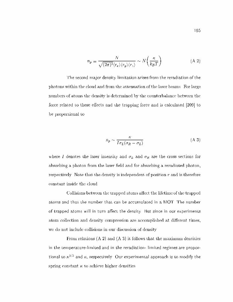
195
np �Np
(2�)3hrxihryihrzi� N
��
kBT
�(A.2)
The second major density limitation arises from the reradiation of the
photons within the cloud and from the attenuation of the laser beams. For large
numbers of atoms the density is determined by the counterbalance between the
force related to these e�ects and the trapping force and is calculated [209] to
be proportional to
np ��
I�L(�R � �L)(A.3)
where I denotes the laser intensity and �L and �R are the cross sections for
absorbing a photon from the laser �eld and for absorbing a reradiated photon,
respectively. Note that the density is independent of position r and is therefore
constant inside the cloud.
Collisions between the trapped atoms a�ect the lifetime of the trapped
atoms and thus the number that can be accumulated in a MOT. The number
of trapped atoms will in turn a�ect the density. But since in our experiments
atom collection and density compression are accomplished at di�erent times,
we do not include collisions in our discussion of density.
From relations (A.2) and (A.3) it follows that the maximum densities
in the temperature-limited and in the reradiation- limited regimes are propor-
tional to �3=2 and �, respectively. Our experimental approach is to modify the
spring constant � to achieve higher densities.

196
Because the spring constant is proportional to the magnetic-�eld gra-
dients @B=@ri, it is desirable to operate the trap at large gradients when aiming
for high densities. However, H�ope et al. [210] observed that increasing the gra-
dients leads to a strong decrease of the loading rate R � (@B=@ri)�14=3 at
which atoms are captured from the vapor gas. They reported a decrease in the
number of trapped atoms from 107 for a normal MOT with �eld gradients of
the order of 10 G/cm down to 10 atoms for a vertical gradient of 207 G/cm. In
contrast, for the measurements described in this paper we �rst collect atoms
from the vapor gas, using low �eld gradients, and then rapidly increase the �eld
gradients. This separation of the collection and the compression processes al-
lows us to achieve high densities for large numbers of atoms.
In addition it can be advantageous to increase the detuning �L of the
trapping laser beams. In the reradiation limit large detunings are expected to
decrease the repelling reradiation forces strongly (� ��4L ), while the decrease of
the trapping force only scales as ��1L in the central, low-magnetic-�eld region of
the trap and as ��3L in the outer region [202, 208]. Thus for a given number of
atoms the new balance between these forces favors higher densities. Although
in the temperature-limited regime larger detunings have been found to lead to
lower temperatures, the actual densities depend on the ratio between the tem-
perature and the (detuning-dependent) spring constant according to relation
(A.2). Steane et al. [202] suggest that the densities in the temperature-limited
regime are in fact independent of detuning.

197
A.3 Experimental Procedure
For trapping 85Rb atoms from a vapor gas we employ the standard
con�guration of a MOT, i.e., three pairs of appropriately polarized counter-
propagating laser beams intersecting in the zero point of a magnetic quadrupole
�eld, which is created by a pair of coils in an anti-Helmholtz con�guration.
Light from a diode laser drives the 5s2S1=2(F = 3) ! 5p2P3=2(F0 = 4) tran-
sition in 85Rb (natural linewidth �=2� = 6 MHz) at a wavelength of 780 nm
with a peak intensity of 15 mW/cm2 in each of the six beams (FWHM beam
size, 7 mm). To provide hyper�ne pumping we overlap the light emitted from
a second laser with the trapping laser beams and repump the atoms on the
5s2S1=2(F = 2) ! 5p2P3=2(F0 = 3) transition. At a measured e�ective sat-
uration parameter of S � 13 we are able to trap up to 108 atoms with a
loading rate of 107 atoms/s. The 1=e time constant for atoms to remain in
the trap under these conditions is 9 s. The number of trapped atoms can be
deduced from measuring a known fraction of the emitted uorescent light on
a calibrated photodiode. The accuracy in determining the absolute number
of atoms is about �20%, whereas the measurements on relative numbers at
a �xed detuning are better than �5%. Information on the size of the cloud
is obtained by observation of the uorescent light with a CCD camera and
analysis of the obtained video pictures of the cloud with a computer. (More
precisely, we store data from only the one horizontal line and the one vertical
line that include the peak of the atom cloud.) The resolution of this detection
scheme is better than 20 �m.
Initially we set the detuning to �9 MHz and the �eld gradient to
@B=@rz(= 2@B=@rx;y) = 11 G/cm to optimize the collection e�ciency of the
198
MOT. After collection for typically 0:5 s, the cloud contains 6�106 atoms and
exhibits horizontal and vertical FWHM sizes of 0:8 and 0:3 mm, respectively,
giving a density of 2 � 1010 cm�3. Note that in the uncompressed MOT the
shape of the cloud and hence also the ratio between the horizontal and the
vertical cloud sizes is signi�cantly distorted by intensity inhomogeneities of
the trapping laser beams. We then jump the detuning to various values. One
millisecond after having jumped the detuning, we ramp the magnetic �eld in
�ve steps over 5 ms to �eld gradients @B=@rz between 11 and 228 G/cm. After
each step the magnetic �eld settles within 0:1 ms. Details of stepping time
and step size are not critical unless the gradient is jumped in a single step;
in this case a signi�cant loss of atoms is observed. After establishing a new
magnetic-�eld gradient, we allow the cloud to equilibrate for 20 ms before we
measure sizes, shapes, and numbers of atoms of the cloud.
A.4 Laser Detuning E�ects
In the measurements described �rst, we concentrate on the in uence
of the laser detuning and do not change the �eld gradients. We collected atoms
from the vapor gas for 0:5 s (! N � 6�106 atoms) and then jumped the laser
detuning from the collection detuning �L = �9 MHz to values of �19, �32,
and �44 MHz at a constant vertical �eld gradient of @B=@rz = 11 G/cm.
We observe that for these low �eld gradients the cloud exhibits an irregular
non-Gaussian shape. Hence the measured sizes and therefore also the densities
in this regime have to be considered estimates. We believe that the irregular
shapes are due to an increased sensitivity to laser �eld inhomogeneities at
lower �eld gradients. When we jump the detuning from �9 to �19 MHz, the

199
cloud sizes decrease to � 0:5 mm (FWHM) in the horizontal plane and � 0:3
mm (FWHM) in the vertical direction. For larger detunings the cloud size
does not decrease any further. Since the number of atoms in the trap stays
approximately constant as the detuning is jumped, the estimated densities
increase by a factor of 3 in going from �9 to �19 MHz (Ref.[211]) but do not
increase for further detuning. The density's insensitivity to detuning above
�19 MHz coincides with the predictions in Ref.[202] for a cloud that is density
limited by its temperature; i.e., for large detunings (4��L � �) the cloud size
should become independent of the detuning [212].
A.5 E�ect of the quadrupole �eld gradient
We now describe measurements in which we ramp the �eld gradient
after we jump the laser detuning to�44 MHz. For this detuning and for vertical
�eld gradients of up to 60 G/cm all atoms are compressed into a narrow peak
that exhibits a Gaussian shape, permitting an accurate determination of the
densities. For @B=@rz > 60 G/cm, however, this narrow peak (central feature)
is surrounded by a di�use cloud of atoms. While the position and the shape
of the di�use cloud strongly depend on the alignment and the imbalance of
the laser beams, the position, the shape, and the size of the central feature
are relatively insensitive to slight misalignment. The existence of the two
parts of the atom cloud and their di�ering behavior is predicted in Refs.[202]
and [208]. This result is consistent with a picture of the central feature's
being compressed by a strong, position-dependent polarization gradient force,
which has been found to be the dominant trapping force for low magnetic
�elds,. i.e., in the trap center. On the other hand, in the large magnetic �elds

200
beyond the trap center this force is suppressed, and only the spontaneous force
remains, which allows the atoms to spread into a sparse cloud. In addition,
even the force of the magnetic �eld on the magnetic moments of the atoms
may be nonnegligible in this region. The precise roles of the individual forces,
however, require further investigation. Figure A.1(a) shows the FWHM of the
central feature in the horizontal and the vertical directions as a function of the
vertical �eld gradient @B=@rz , for the detuning of �L = �44 MHz. The data
follow the dependence expected from Eq. (A.1) for a constant temperature,
i.e., hrii � (@B=@ri)�1=2, and the ratio of the sizes in the horizontal and the
vertical directions is close top2 (see the dashed curves in Fig. A.1). The
fraction of atoms in the central feature can be estimated from the video data,
and the total number of atoms in the trap is deduced from the photodiode
signal. For the detuning of �44 MHz we observe no measurable decrease of
the total number of atoms during compression, and the lifetime of the atoms in
the CMOT is found to be of the order of seconds. Although the total number
of atoms stays approximately constant as the magnetic- �eld gradient changes,
the fraction of atoms in the central feature starts to decrease for gradients
larger than 60 G/cm [Fig. A.1(b)]. Knowing the total number of atoms, the
Gaussian width of the central feature, and having estimated the fraction of
atoms in the central feature, we calculate the peak density np shown in Fig.
A.1(c) as a function of the vertical magnetic-�eld gradient. For �elds smaller
than 60 G/cm, peak densities as high as 5 � 1011 cm�3 have been achieved.
This corresponds to an increase in density of more than an order of magnitude
compared with the density of a normal MOT (np � 2� 1010 cm�3). We point
out that for this large detuning the CMOT exhibits high densities with long
lifetimes and Gaussian density distributions; therefore it is an ideal tool to use
201
in studies that require high densities and for which a precise knowledge of this
density is desirable, such as investigations of cold collisions[204].
Analogous measurements have been performed with smaller detun-
ings of �9 (i.e., the normal MOT detuning), �19, and �32 MHz. In general
we �nd lower densities and less Gaussian-shaped curves in these cases. These
deviate signi�cantly from the magnetic-�eld gradient dependence expected for
the temperature-limited sizes � (@B=@ri)�1=2 as well as for reradiation-limited
sizes � (@B=@ri)�1=3. On the other hand, we observe that the sparse cloud sur-
rounding the central feature diminishes with decreasing detuning. In addition,
we �nd that the total number of atoms remaining in the trap after compression
also decreases; for the smallest detuning and the largest �eld gradient this loss
amounts to 65%. The loss of atoms occurs on two time scales: a rapid loss of
atoms, which is not yet understood, is observed mainly during compression,
followed by a slow decay with time constants between � 50 ms (@B=@rz = 228
G/cm, �L = �9 MHz) and seconds (both the rapid loss and the slow decrease
become less pronounced with larger detunings and smaller gradients). The slow
loss of atoms is likely to be caused by intratrap collisions, which are dependent
on the laser detuning in a manner consistent with light-assisted collisions [102].
In any case the lifetime of the CMOT would be plenty long enough to allow
for the transfer of the compressed atom cloud to a purely magnetic trap, in
which there would be no light-assisted collisions and where further cooling, for
instance, by evaporation [213], seems feasible.

202
Figure A.1: (a) Horizontal and vertical sizes, (b) number of atoms, and (c) peak
densities shown as a function of the vertical magnetic �eld gradient @B=@rz(= 2@B=@rx;y). The detuning was set to -44 MHz. The �lled symbols in (b)
and (c) represent the actual parameters of the cloud, and the open symbols
are an estimate of the fraction of atoms in the central feature and the peak
densities connected to this estimated fraction (see text). The dashed curves
in (a) are a �t to an inverse-square-root dependence with a forced ratio ofp2
between the radial and the axial sizes. Figure taken from Ref. [19].

203
A.6 E�ect of changing the number of atoms in the trap
In a further series of measurements the collection time � and hence
the total number of atoms is varied from � = 0:1 s to � = 30 s, corresponding
to 3�106 � N � 8�107. After collection of the atoms the detuning is jumped
to �L = �32 MHz, and the magnetic �eld gradient is ramped to @B=@rz = 85
G/cm. We �nd that both the sizes hrii [Fig.A.2(a)] and the number of atoms in
the central feature Ncf (Fig.A.2(b)] increase for small total numbers of atoms
N in the trap. Analyzing the data yields a dependence of hrii � 3
pNcf , which is
expected in the reradiation-limited regime according to relation (A.3); in fact,
the densities derived from the shown sizes and numbers are approximately
equal and amount to n � 2 � 1011 cm�3 [Fig.A.2(c)]. For N � 2 � 107 any
additionally loaded atoms are dispersed into the sparse cloud around the central
feature, so the number of atoms in the central feature as well as its size do
not increase any further. We believe that the limit on the size of the central
feature, and therefore on the number of atoms compressed therein, arises from
a suppression of polarization gradient forces for large radii. As is mentioned
above, the dominant role of these forces in the center of an ordinary MOT
is pointed out in Refs. [202] and [208]. Steane et al. [202] suggest that the
high gradients, however, give rise to Larmor frequencies, which then become
comparable with the optical pumping rate and the ac Stark shifts at radii small
enough to be inside the actual cloud. The occurrence of large magnetic �elds
close to the trap center will inhibit the polarization-gradient forces even at these
small radii, and in this way could lead to a limitation of the size of the strongly
compressed central feature. We �nd the size limit of the central feature and
the existence and properties of the di�use cloud an intriguing problem worthy

204
of further theoretical as well as experimental studies.
A.7 Conclusion
In summary, we have investigated the behavior of an atom cloud in
a magneto-optical trap that is suddenly exposed to high magnetic-�eld gradi-
ents. We have studied sizes and shapes of the atom cloud as a function of the
amplitude of the magnetic-�eld gradient, of the laser detuning, and of the total
number of atoms. For large detunings and intermediate �eld gradients, peak
densities as high as 5 � 1011 cm�3 are achieved, corresponding to a density
increase of more than an order of magnitude compared with the density of a
normal MOT. Although this density increase is in principle of a transient na-
ture, we observe lifetimes of the order of seconds for large detunings. Moreover,
we �nd that the density distribution in this highly compressed MOT is purely
Gaussian for large detunings and intermediate �eld gradients. Therefore in this
regime the CMOT appears to be an ideal tool for investigations that require
an accurate knowledge and high values of the density, such as studies of cold
collisions. Furthermore, �rst measurements indicate that the transfer of atoms
from the normal MOT into a magnetic trap can be signi�cantly improved by
this method of compression. The resulting high densities in the magnetic trap
are an important step toward the goal of evaporative cooling in the magnetic
trap, which might eventually lead to the observation of collective e�ects such
as Bose-Einstein condensation of the weakly interacting atom sample [203].

205


![Bose-Einstein Condensation with High Atom Number in a Deep ... · Bose-Einstein condensation was predicted in 1925 [Bose, 1924, Einstein, 1925], at the time when quantum mechanics](https://img.pdfslide.us/doc/110x75/5f0235fc7e708231d4031fe6/bose-einstein-condensation-with-high-atom-number-in-a-deep-bose-einstein-condensation.jpg)


![AVALANCHES IN A BOSE-EINSTEIN CONDENSATE · 1.4.1.1 BOSE-EINSTEIN CONDENSATION The realization of Bose-Einstein condensation in dilute gases in 1995 [1] was a milestone in the rapidly](https://img.pdfslide.us/doc/110x75/5f0235fc7e708231d4031fe8/avalanches-in-a-bose-einstein-condensate-1411-bose-einstein-condensation-the.jpg)