Embed Size (px)
Citation preview

No. 2001-16
THE FINANCING OF INNOVATION: LEARNING ANDSTOPPING
By Dirk Bergemann and Ulrich Hege
February 2001
ISSN 0924-7815
The Financing of Innovation:
Learning and Stopping∗
Dirk Bergemann† Ulrich Hege‡
November 2000
Abstract
This paper considers the financing of a research project under uncertainty about the time of comple-
tion and the probability of eventual success. The uncertainty about future success gradually diminishes
with the arrival of additional funding. The entrepreneur controls the funds and can divert them. We
distinguish between relationship financing, meaning that the entrepreneur’s allocation of the funds is
observable, and arm’s length financing, where it is unobservable.
We find that equilibrium funding stops altogether too early relative to the efficient stopping time in
both financing modes. We characterize the optimal contracts and equilibrium funding decisions. The
financial constraints will typically become tighter over time under relationship finance, and looser under
arm’s length financing. The trade-off is that while relationship financing may require smaller information
rents, arm’s length financing amounts to an implicit commitment to a finite funding horizon. The lack of
such a commitment under relationship financing implies that the sustainable release of funds eventually
slows down. We obtain the surprising result that arm’s length contracts are preferable in a Pareto sense.
Keywords: innovation, venture capital, relationship financing, arm’s length financing, learning, time-
consistency, stopping, renegotiation, Markov perfect equilibrium.
JEL Classification: D83, D92, G24, G31.
∗ The authors would like to thank Dilip Abreu, Patrick Bolton, Amil Dasgupta, Thomas Hellmann, Godfrey Keller, Georg
Noldeke, Kjell Nyborg, Ted O’Donoghue, David Pearce, Paul Pfleiderer, Rafael Repullo and Luca Rigotti for many helpful
comments and suggestions. Seminar participants at Basel, Budapest, LSE, Mannheim, Princeton, Rotterdam, Stockholm,
Tilburg, Econometric Society Winter Meetings’98 and EFA’99 provided stimulating discussions. The first author gratefully
acknowledges financial support from the National Science Foundation (SBR 9709887) and an A.P. Sloan Research Fellowship,
the second author from a TMR grant of the European Commission.† Department of Economics, Yale University, New Haven, CT 06511, E-mail [email protected], Phone 1-203-432
3592.‡Department of Finance, ESSEC Business School and CEPR, 95021 Cergy-Pontoise Cedex, France, E-mail [email protected],
Phone 33 1 3443 3239.
1

1 Introduction
Typically, when decisions are made to start an R&D project or an innovative venture, much uncertainty
subsists about the time and capital needed until the research is completed, and more generally about the
chances of the project to succeed. This uncertainty is a source of potential conflict between the parties
involved, mainly the financiers providing the capital and the researchers or entrepreneurs carrying out the
project. They may make it difficult to define enforceable and mutually satisfactory contract terms, and
encumber the effort to secure the necessary funding.
The research and development process for a new pharmaceutical product may serve as an illustration.
The idea for a new drug is most likely based on some initial and very preliminary research. The development
itself requires substantial investments before the value of the initial idea can be assessed. More information
will be produced over time as to whether the project will be successful or should be abandoned due to poor
results. The time and money spent until the research is completed successfully remain uncertain. And as
researchers obtain negative signals, they may be liable to withhold information from management, be it
because they are (over-) confident or because they rationally try to prolong the search.
Contracting problems of this kind are likely to create obstacles for the efficient funding of research as
exemplified by the following three areas. First, they will affect venture capital firms financing high-tech start-
ups. Empirical research on the venture capital industry reveals that venture capitalists are well aware of such
problems, and that they go to great length to build possible safeguards into their contracts.1 Second, the
optimal financing of research is also a concern for the capital budgeting for R&D expenditures process within
a firm. Third, the problems that we investigate arise also for governments, universities, research foundations
and other organizations that sponsor research. They need to evaluate progress of research projects and to
determine the timing for grant renewal or the decision to abandon.
This paper examines the funding of a research project, essentially an idea owned by an entrepreneur,
in the presence of uncertainty about the merit of the idea and about the time until completion. To find
out about the nature of the project and to save the chances for successful realization, a constant flow of
funds needs to be injected. The entrepreneur is wealth-constrained and must raise the funds from outside
investors. Uncertainty is represented by a simple stochastic process. If the project is promising and funds are
injected, then there is a positive probability in every period that the project will be completed successfully.
This probability is equal to zero if the project is a failure. The entrepreneur can ask for new funds in every
period and the time horizon itself is infinite. The development of the project initiates a Bayesian learning
process as continued lack of success will lead to a downgrading of the belief about the nature of project.
The project ends either with a success, or it will eventually be abandoned in the light of persistent negative
news.
The entrepreneur controls the allocation of the funds. She can choose to invest the funds efficiently into
the project or to divert them to private ends. This agency conflict is rich because of the dynamic nature of
the investment problem. When diverting the funds, the entrepreneur not only enjoys the immediate benefit
1For example the following instruments (documented in Sahlman (1990), Hellmann (1998), Kaplan and Stromberg (1999)
and Gompers and Lerner (1999)): Venture capitalists retain extensive control rights, in particular rights to claim control on
a contingent basis and the right to fire the founding management team; they keep hard claims in form of convertible debt or
preferred stock, underpinning the right to claim control and abandon the project; and staged financing and the inclusion of
explicit performance benchmarks make it possible to fine-tune the abandonment decision.
2

from consuming the money meant for investment. She can also secure the option of continued funding in
the future, since nothing can be learned about the project when the funds are not invested as supposed, and
since the project remains a positive net present value project all the same, meaning that the entrepreneur
can go back to the financier and solicit another round of funding. Thus, the entrepreneur’s discretion over
the funds is intimately linked to the timing of the abandonment decision.
As for the entrepreneur’s decision to invest or divert the funds, we shall make a distinction according to
whether the action is observable or unobservable.2 If the action of the entrepreneur is observable, it is in
fact “observable, but not verifiable” as it is usually described in the incomplete contracts literature. The
information about the future likelihood of success is then always shared by entrepreneur and investor and the
environment is at all times one of symmetric information. We liken this situation to relationship financing
since the investor needs to keep a hands-on approach on the project to stay informed. With unobservable
actions by the entrepreneur, we are investigating a standard moral hazard problem between investor and
entrepreneur. As the investor is uncertain whether the entrepreneur did or did not exert effort in the past
period, a situation of asymmetric information arises how to assess the true probability of future success. We
refer to this situation as arm’s length financing.
We develop the model first in discrete time and then consider the continuous time limit as the time
elapsed between any two periods converges to zero. This approach has the advantage that we can adopt
standard equilibrium definitions and discuss the decisions and belief updates in discrete time, yet obtain
explicit solution for equilibrium policies and values through differential equations which represent the dy-
namic programming equations. In the equilibrium analysis, we examine whether the funds are released at
the efficient rate by the investor and whether the project is abandoned at the efficient stopping point. We
further investigate how entrepreneur and investor share the proceeds of the project as a function of the
elapsed time and received funding until the completion of the project.
We first consider the environment with relationship financing (observable actions). The information about
the project is then always common for both parties and funding renewal is negotiated under symmetric in-
formation. We find that there is a unique Markov perfect equilibrium of the contracting game. Alternatively,
we relax the Markov assumption and merely impose that the equilibrium be weakly renegotiation-proof in
the sense of Farrell and Maskin (1989), meant to capture the inability of entrepreneur and investor to prevent
recontracting or renegotiation. It is shown that the unique equilibrium is identical to the equilibrium derived
under the Markov assumption.
The basic conflict between entrepreneur and investor can be described as follows. For the entrepreneur,
the project represents the possibility to win a single large prize. Yet as long as she can attract funding for
it, the project also constitutes a stream of rents provided by the funds which she could divert to her private
ends. The tension between investing and diverting the funds is accentuated by the fact that the successful
completion of the project automatically stops the flow of funds. The direct incentives for the entrepreneur
then have to be adequate to offset the possible loss in future rents, hence they have to be increasing in the
volume of future funding the entrepreneur expects to obtain in equilibrium. Yet as the project goes on and
the outlook becomes less promising, the participation constraint of the investor eats more and more into
the expected cash flow of the project, leaving less and less for the direct incentive of the entrepreneur. At
some point, this residual will fall short of what is needed to provide incentives. The only possible solution
2We would like to thank Patrick Bolton for a suggestion to include this distinction.
3

is that the investor slows down the release in funds, which happens in the form of probabilistic funding
decisions by the investor. This reduces the entrepreneur’s option value of prolonging the project, and the
incentive constraint can be met again. As time goes on and the posterior belief decreases, the slow down
in funding becomes more serious, and funding will come down to a trickle as the belief approaches the final
abandonment point. Funding ceases altogether too early relative to the efficient policy.
As we consider the case of arm’s length financing (actions are unobservable), we need to take into account
the dynamics of the moral hazard problem. The moral hazard problem about the entrepreneur’s decision
in the current period translates into an adverse selection problem about beliefs in future periods. For the
entrepreneur, control over the investment flow means also control over the information flow. Hence, the
private beliefs of entrepreneur and investor about the project can diverge. To facilitate the comparison with
the earlier results, we characterize first the Markov sequential equilibrium which is unique. We show that
the Markov restriction is in fact superfluous, as the asymmetric information implies that funding will be
stopped in finite time, and the outcome can be solved by backwards induction.
We find that while the tension between immediate incentives and intertemporal rents remains, there
is one subtle, yet important difference in the value of a deviation for the entrepreneur. With symmetric
information, the entrepreneur could renew his proposal after a deviation based on the belief held in the
previous period, since nothing in the perception of the project has changed on either side. In contrast, with
unobservable actions, the investor will automatically downgrade his belief after a deviation and insist in the
continuation game to be compensated on the basis of his belief, which is more pessimistic than warranted.
This change in the belief limits the maximal financing horizon, which relaxes the incentive constraint and
facilitates funding. On the other hand, the entrepreneur commands an additional information rent since she
controls the information flow.
The unobservability of the action may also affect the evolution of funding over time through the recursive
nature of the incentive problem. As funding towards the end of the project occurs now more frequently, the
entrepreneur may find herself more tempted to postpone investment at the beginning of the project’s lifetime.
This problem is particularly acute for projects with a very long funding horizon, that is projects where the
initial assessment is sufficiently good to warrant patient investment. These ‘rich’ projects may have to be
started with a slow rate of funding and observe a gradual increase in the funding rate as time elapses. The
change in the evolution of the funding rate is a consequence of the recursive incentive constraints, which
differ for observable and unobservable actions.
We briefly discuss the robustness of our assumptions for both environments, with observable and with
unobservable actions, notably by allowing for a redistribution of the bargaining power to the investor and
the possibility of long-term contracts that commit the investor to a certain course of funding. These changes
may improve the allocation to the extent that they reduce the entrepreneur’s future rents, but confirm the
thrust of the analysis.
We finally compare arm’s length and relationship financing. We identify the following basic trade-off:
Under relationship financing, there is no informational asymmetry, and the information rent that compen-
sates the entrepreneur for her control of the information flow can be saved; but under arm’s length funding,
the investor is committed to stick to a finite stopping time, reducing the option value of the entrepreneur to
prolong the project through deviations. We find that the second effect always dominates and arm’s length
contracts allow for a higher project value.
4

Our paper is related to a strand of the financial literature that looks at (static) agency problems linked
to entrepreneur’s discretion to influence the stopping decision. Qian and Xu (1998) observe that soft budget
constraint problems of this kind are endemic in bureaucratic systems of R&D funding, which may help explain
the secular demise of these systems. Cornelli and Yosha (1999) emphasize the possibility to window-dress
performance signals to have the project continued. Dewatripont and Maskin (1995) note that having multiple
investors may be a device to mitigate this problem. The choice whether research activities financed externally
or in-house may be determined by this problem (Ambec and Poitevin (1999)). Other papers investigate the
instruments of the venture capital financing with regard to moral hazard and stopping problems, like stage
financing and the use of convertible securities (e.g. by Repullo and Suarez (1999)) and the possibility to fire
incumbent management (Hellmann (1998)). All of these proposals refer to purely contractual instruments,
though. Since contracts can be renegotiated, the question then arises what happens if no time-consistent
commitment to stop is available. This is the starting point of our paper.
There is also a connection between our paper and the literature on the strategic default problem in
incomplete financial contracts, that is the problem of borrowers refusing to honor obligations in spite of
being solvent (Hart and Moore (1994, 1998), Bolton and Scharfstein (1996), Neher (1999)). Only incentive
contracts offering a stick in form of liquidation if there is such a strategic default, and a carrot in form of more
future profits if the contract is honored, can work. In these models, cash flows are received in intermediate
periods, and strategic default (weakly) reduces the value of future cash flows. In our model, only one cash
flow - but at an uncertain time - is received, and diverting funds increases the value of future periods. In
this literature, Gromb (1994) is closest to our model. Analyzing a (finite or infinite) repetition of projects a
la Bolton and Scharfstein (1996), he shows that the repeated nature of the game severely impinges on the
efficiency of feasible contracts.
Bergemann and Hege (1998) analyze a limited version of the present model from the narrower perspective
to derive implications for venture capital contracting. This paper extends and generalizes the analysis (i)
by considering stopping decisions that are renegotiation-proof or recontracting-proof, and (ii) by taking into
account observable, but unverifiable actions.
The paper is organized as follows. The model is formally presented in Section 2, where we also derive
the socially efficient funding policy in a discrete time framework. The equilibrium analysis begins in Section
3 by considering observable actions by the entrepreneur. Section 4 examines equilibrium financing when the
allocation decision of the entrepreneur is unobservable to the investor. Both sections end with a discussion of
the robustness of the equilibrium results to different bargaining and contracting assumptions. The structure
and efficiency of the equilibria under symmetric and asymmetric information are compared in Section 5.
Section 6 presents some concluding remarks.
2 The Model and First-Best Policy
The project, the investment technology and the evolution of the posterior beliefs are described in Subsection
2.1. We begin in discrete time and then describe the transition to continuous time. In Subsection 2.2, we
introduce the contracting problem. In Subsection 2.3, we derive the efficient stopping time and the first-best
value of the project.
5

2.1 Project with Unknown Returns
We begin by developing the model in discrete time. Time periods are denoted by t = 0, 1, ...,∞, and thediscount factor is δ ∈ (0, 1). The entrepreneur owns a project with unknown returns. The project is either“good” with prior probability α0 or “bad” with prior probability 1 − α0. If the project is “good”, then at
every t, the project is successfully completed with probability λ and yields a fixed positive payoff R. The
success probability λ requires an investment flow of cλ in every t. If the project is “bad”, then it will never
yield a positive return and the probability of success is zero independent of the investment flow.
The uncertainty about the project is resolved over time as the flow of funds either produces a success or
leads to a stopping of the project. The investment process is like an experiment which produces information
about the future likelihood of success. The current information is represented by the posterior belief αt that
the project is good. The evolution of the posterior belief αt, conditional on no success in period t, is given
by Bayes’ rule as a function of the prior belief αt and the investment flow λ:
αt+1 =αt (1− λ)
1− λαt. (1)
The posterior belief αt decreases over time if success doesn’t arise. The decline in the posterior belief is
stronger for larger investments flows λ as the agents become more pessimistic about the likelihood of future
success. The posterior belief changes only slowly for very precise beliefs about the nature of the project,
i.e. if αt is either close to 0 or 1. Correspondingly, the event of no success is most informative with diffuse
beliefs, or when αt is close to12 .
Next we consider the transition to continuous time, by defining ∆ to be the time elapsed between periods
t and t+∆ and consider the limit as ∆→ 0. The discount factor δ between any two periods is then given
by
δ =1
1 + r∆,
where r is the discount rate. The probability of success conditional on the project being good is now given
by ∆λ. The evolution of the posterior probability αt+∆ is consequently given by:
αt+∆ =αt (1−∆λ)1− αt∆λ
,
or
αt+∆ − αt = −αt+∆ (1− αt)∆λ,
which leads to the following differential equation as ∆→ 0,
dα (t)
dt= −λα (t) (1− α (t)) . (2)
For all variables, we use a subscripted t to indicate discrete time and a parenthetical (t) to indicate the
continuous time limit.
2.2 Contracting
The entrepreneur has initially no wealth and seeks to obtain external funds to realize the project. Financing
is available from a competitive market of investors, which is represented in the model by a single investor
6

who can only accept or reject contract proposals by the entrepreneur. Entrepreneur and investor share
initially the same assessment about the likelihood of success represented by the prior belief α0. The funds
are supplied by the investor and the entrepreneur controls the allocation of the funds. She can either invest
the funds into the project or divert the capital flow to her private ends.3 The entrepreneur is protected by
limited liability, i.e. her payoff can never be negative.
The time structure in every period t is as follows. At the beginning of period t the entrepreneur can offer
the investor a share contract st ≥ 0. The share st represents the share of the entrepreneur in the proceeds ifthe project succeeds in period t. The investor receives the remaining share 1 − st. The restriction to sharecontracts is without loss of generality due to the binary nature of the project. After the contract proposal,
the investor can decide whether to accept or reject the new contract. If he accepts the contract, then he
provides the entrepreneur with the necessary funds cλ in period t to support the development of the project.
If he rejects the contract, then a new proposal can be made by the entrepreneur in the subsequent period.
Finally, and conditional on funding, the entrepreneur decides whether to invest the funds in the project or
divert them to her private ends.
t t+ 1−−−−−−−−−−−−−−−−−−−−−−−−−−−−−−−−−−−−−−−−−−−−−−−−−−−−−−−−−−−−−−−→x x x xE offers st I offers 0 or λ E invests or diverts realization 0 or R
Figure 1: Timeline of Events
Initially we shall assume that the investment decision of the entrepreneur, or simply her ‘action’, is
observable but not verifiable to the investor. In contrast, in the second part of the paper, we shall investigate
the case of unobservable actions by the entrepreneur. In any case, the investment decision of the entrepreneur
is not contractible and hence not enforceable by the investor. The following notation pertains to the model
with observable actions, and the necessary modifications for the case of observable actions follow in due
course.
Formally, let Ht denote the set of possible public histories up to, but not including period t. A proposal
strategy by the entrepreneur is given by:
st : Ht → R .
A decision rule by the investor, possibly randomized, is a mapping from the history and the contract proposal
into a binary decision to reject (dt = 0) or to accept (dt = 1):
pt : Ht × st → ∆ {0, 1}
The probability of acceptance at (ht, st) is denoted by p (ht, st).4 Finally, an investment policy by the
entrepreneur is given by:
it : Ht × st × dt → {0,λ}3The model permits an equivalent and perhaps more standard formulation of the agency problem: the efficient application
of the investment requires effort, which is costly for the entrepreneur. By reducing the effort, the entrepreneur also reduces the
probability of success and hence the efficiency of the invested capital. In both cases, a conflict of interest arises about the use
of the funds.4The restriction to pure strategies with respect to the offer and investment decision by the entrepreneur is without loss of
generality.
7

A generic public history of the game is denoted by ht ∈ Ht and is simply a realized sequence of offers, fundingand investment decisions:
ht = {s0, ...., st−1; d0, ...., dt−1; i0, ..., it−1} .The evolution of the posterior belief αt is not included in the history as it can be inferred from Bayes’ rule
and the sequence of public funding and investment decisions. By default, updating occurs only conditional
on failure of the project as the game ends as soon as the project is completed successfully. Thus given any
prior α0, an arbitrary history ht uniquely determines the current posterior belief αt = α (ht).
2.3 First-Best Policy
We begin with an analysis of the socially optimal investment policy. The project should receive funds as
long as the expected returns of the investment exceed the cost, or
αtλR− cλ ≥ 0. (3)
It follows that the project should receive its final investment at the lowest αT where the current net return
is positive:
αTλR− cλ ≥ 0, (4)
while any further investment, conditional on failure today, would display negative net returns:
αT+1λR− cλ < 0, (5)
where αT+1 is computed by Bayes’ rule as in (1). The stopping condition in the discrete time model is then
described by the inequalities (4) and (5). This inequalities will coincide in the continuous time limit and
collapse to the equality:
αTλR− cλ = 0.The social value of the project, denoted by V (αt), is given by a familiar dynamic programming equation:
V (αt) = max {αtλR− cλ+ δ (1− λαt)V (αt+1), 0} . (6)
The value of the program can be decomposed into the flow payoffs and continuation payoffs. The flow payoffs
are the returns multiplied by the current probability of success minus the investment costs. The continuation
payoffs arise conditional on no success, or with probability (1− αtλ), in which case the future is assessed
at a new posterior, namely αt+1. The efficient stopping conditions (4) and (5) can be recovered from the
dynamic programming equation at αT by setting V (αT+1) = 0.
As we consider the transition to continuous time, the social problem in t can be written, using the earlier
∆ notation, as:
V (αt) = max
½αt∆λR− c∆λ+ (1−∆λαt)
1 + r∆V (αt+∆), 0
¾.
After multiplying with (1 + r∆) and dividing by ∆, we obtain
rV (αt) = max
½(1 + r∆)αtλR− cλ+ V (αt+∆)− V (αt)
∆− λαt1 + r∆
V (αt+∆), 0
¾,
8

and as we take the limit as ∆→ 0:
rV (α (t)) = max {α (t)λ (R− V (α (t)))− cλ+ α0 (t)V 0 (α (t)) , 0} .. (7)
The flow expected return in period t is α (t)λR and the flow costs are cλ. As the probability of success
is α (t)λ, the implicit cost of success is that the project is stopped and no further return can be expected.
On the other hand if no success is observed in period t, then the value of the program is changing as the
posterior belief is decreasing. The socially optimal stopping point in continuous time is given by the smooth
pasting conditions:
V (α∗) = V 0 (α∗) = 0,
which determine the efficient stopping point α∗ as expected:
α∗λR− cλ = 0 ⇔ α∗ =c
R. (8)
The stopping point is characterized by the posterior belief in (8). For any given prior belief α0 there is a
one-to-one relationship between the stopping point α∗ and the stopping time T ∗ which expresses the samepolicy in terms of real time:
T ∗ , max½t
¯α0e−λt
α0e−λt + (1− α0)≥ α∗
¾.
Evidently, the optimal stopping time T ∗ depends on the prior belief α0 at which the project is started.The dependence on α0 is suppressed for notational convenience. The stopping time T
∗ represents the timeelapsed between starting at α0 and arriving at the posterior belief α
∗ (under the assumption of a sociallyoptimal constant investment flow cλ). We summarize these results.
Proposition 1 (Optimal Investment Policy)
1. The optimal policy is to invest cλ until T ∗.
2. The social value of the project is:
V (α0) = α0λ (R− c) 1− e−T∗(λ+r)
λ+ r− (1− α0) cλ
1− e−rT∗r
. (9)
The value function V (α0) presents an intuitive decomposition of the value of the project. The first term
in (9) is the expected value of the project conditional on the project being good. Notice that the value of the
project is discounted at a rate which compounds the pure discount rate r and the probability of discovery λ
which results in the factor r+λ. The second term captures the case that the project is bad which occurs with
probability (1− α0). In this case, costly experimentation will continue with probability 1 until the stopping
time T ∗ is reached.We observe in this context that the characterization of the stopping problem (as well as all equilibrium
results) would remain unchanged if the probability of success λ would be a continuous variable with λ ∈ £0, λ¤and the cost of a conditional success probability λ a linear function of λ:
c(λ) = cλ, c > 0.
Due to the linear cost and probability structure, all results would then remain unchanged after replacing λ
by its upper bound λ.
9

3 Relationship Financing
In this Section, we analyze contracting with symmetric information, that is the entrepreneur’s actions are
observable (but not verifiable) for the investor. We refer to this situation as relationship financing. The
notion of subgame and Markov perfect equilibrium are defined in Subsection 3.1. The properties of the
Markov perfect equilibrium are investigated in Subsection 3.2. It is then shown in Subsection 3.3 that the
Markov perfect equilibrium coincides with the weakly renegotiation proof equilibrium. Finally, in Subsection
3.4 we discuss how the contracting results would be affected if the agents could commit to long-term contracts
yet could recontract in every period.
3.1 Equilibrium
In the environment with observable actions, the information of entrepreneur and investor is symmetric in
every period. For a given triple {st, dt, it}∞t=0 of strategies, denote the value function of the entrepreneurat the beginning of period t by VE (ht) and the value function of the investor by VI (ht). The continuation
value in any period after a contract offer st, a funding decision dt and investment decision it are denoted by
VE (st |ht ), VI (st, dt |ht ), and VE (st, dt, it |ht ), respectively.
Definition 1 (Subgame Perfect Equilibrium)
A subgame perfect equilibrium (SPE) is a sequence of policies
{s∗t , d∗t , i∗t }∞t=0 ,
such that for all ht the following inequalities hold:
VE (s∗t |ht ) ≥ VE (st |ht ) , for all st;
VI (st, d∗t |ht ) ≥ VI (st, dt |ht ) , for all st and dt;
VE (st, dt, i∗t |ht ) ≥ VE (st, dt, it |ht ) , for all st, dt and it.
The three inequalities in the definition of the equilibrium are necessary as offer, acceptance and investment
decision occur sequentially in any given time period t. We restrict our attention initially to Markovian
equilibria where strategies are allowed to depend only on the payoff relevant history of the game, which are
here represented by the posterior belief αt in every period t.
Definition 2 (Markov Perfect Equilibrium)
A Markov perfect equilibrium (MPE) is a subgame perfect equilibrium
{s∗t , d∗t , i∗t }∞t=0 ,
such that the sequence of policies satisfies ∀ht ∈ Ht, ∀h0t0 ∈ Ht0 , ∀st, s0t0 , ∀dt, d0t0 :
α (ht) = α (h0t0) ⇒ s∗t (ht) = s∗t0 (h0t0) ;
α (ht) = α (h0t0) , st = s0t0 ⇒ d∗t (ht, st) = d∗t0 (h
0t0 , s
0t0) ;
α (ht) = α (h0t0) , st = s0t0 , dt = d
0t0 ⇒ i∗t (ht, st, dt) = i∗t0 (h
0t0 , s
0t0 , d
0t0) .
(10)
10

The particular history ht may differ from the one expressed by h0t0 either because they pertain to twodifferent dates t = t0, and/or because they specify different past realizations. Since the moves in any periodare sequential, the relevant state for the investor is not only the belief about αt but must also include the
entrepreneur’s contract offer. Likewise, for the entrepreneur’s final allocation decision, the state description
needs to be augmented by her own contract offer and the investor’s approval decision.
3.2 Analysis
Consider the situation of the investor at an arbitrary point of time. He receives a proposal by the entrepreneur
to fund a project for the current period in exchange for shares in the proceeds of the project should it succeed
in the current period. As the current contract commits neither investor nor entrepreneur to any future course
of action, the investor is willing to accept the proposal as long as the expected returns are non-negative, or
α (t) (1− s (t))λR ≥ cλ. (11)
The inequality then represents the participation constraint of the investor. However, the expected returns
can only materialize if the entrepreneur decides to put the funds to work in the project, rather than to divert
them to her private ends. This is the incentive problem of the entrepreneur. Consider first what would
happen if the entrepreneur would only get a single chance to realize the project, and this chance would arise
at the belief α = α (t). She would then have to choose between investing and diverting, or
α (t) s (t)λR ≥ cλ. (12)
Jointly, the inequalities (11) and (12) imply that for any funding to occur in equilibrium the expected flow
return from the investment must cover both the cost of the funds for the investor and the opportunity costs
for the entrepreneur, which are represented by the utility arising from a diversion of the funds:
α (t)λR ≥ 2cλ.
The critical posterior belief at which funding will certainly cease is therefore given by
αS ,2c
R,
which is larger than the efficient stopping belief α∗, as αS = 2α∗.The previous argument, however, relied on the assumption that the entrepreneur would only be given a
single chance to realize the project. Yet as the investor cannot commit himself to stop funding the project as
long as a funding proposal leaves him with nonnegative returns, the incentive constraint for the entrepreneur
has to take into account her future opportunities. This can be represented in terms of her value function:
α (t)λ [(s (α (t))R− VE(α (t))] + α0 (t)V 0E (α (t)) ≥ cλ. (13)
The derivation of the equilibrium value function is based on the discrete time model similar to the con-
struction of the social value function earlier in Section 2. The details are presented in the proof of the next
theorem. For any contract s (α (t)), the entrepreneur can either invest the funds or divert them to her private
ends. If the project succeeds in period t, then the returns are given by s (α (t))R, but as they occur at the
11

cost of stopping the project, and therefore foregoing the realization of any future benefit, have to be adjusted
by VE (α (t)).. If the project fails in the current period, then the posterior belief declines and induces changes
in the net value for the entrepreneur, or α0 (t)V 0E (α (t)). The alternative action for the entrepreneur is tosimply divert the funds today and then face a similar problem tomorrow as the state of the project remains
unchanged. Therefore, the equilibrium can be characterized by a sequence of participation constraints for
the investor (as in (11)) and a sequence of incentive constraints for the entrepreneur (as in (13)).
As the entrepreneur will never leave the investor with more than necessary, the equilibrium share s∗ (α (t))is determined by the exact fulfillment of the participation constraint, or
s∗ (α (t)) =a (t)R− cα (t)R
. (14)
We refer to contracts which leave the investor with zero net utility as break-even contracts. As the share
s (α (t)) determines the payoff flow to the entrepreneur, one is lead to ask whether the incentive constraint (13)
can be satisfied for all α (t) ≥ αS . Using (14), we may rewrite the incentive constraint for the entrepreneur
as follows:
α (t)λR ≥ 2cλ+ α (t)λVE (α (t))− α0 (t)V 0E (α (t))). (15)
Here we observe that as VE (α (t)) ≥ 0 and α0 (t)V 0E (α (t))) ≤ 0, the incentive constraint can only be satisfied,for α (t) approaching αS , if α (t)λVE (α (t))− α0 (t)V 0E (α (t))) converges to zero at an appropriate rate. Asthe expected flow of benefits conditional on funding is given by (14), this implies that the only instrument
which can still control the evolution of the payoff is the rate at which funding is provided. In particular as
α (t) converges to αS , this requires that funding is provided only probabilistically and at a decreasing rate.
By considering the deviation option of the entrepreneur, the need to slow down funding becomes even clearer.
Now the entrepreneur can always guarantee herself at least cλ if funding occurs with certainty. Therefore,
continued funding would imply that the value for the entrepreneur would have to be (at least) equal to cλr .
This is the payoff the entrepreneur could guarantee for herself if she were to divert the funds in every period,
thereby pretending that the project is restarted perpetually at an unchanged posterior belief α.
Since the value of the entrepreneur can never exceed the social value of the project, it follows that the
value of the diversion option has to decline. The only way to achieve this is through a slower release of
funds, suggesting that the funding probability decreases as α (t) and hence as the social value of the object
decreases. Within the context of Markovian strategies the funding probability is denoted by p (α (t)). If the
probability is less than one, then participation constraint (11) as well as incentive constraint (13) have to be
satisfied as equalities. For if either one is an inequality, the investor could be induced to provide funds with
probability one.
This leaves the question open whether funding will ever be provided with certainty. To answer this
question, it is helpful to consider the limit case of the incentive constraint (15) as α (t) converges to 1. In
this case, the changes in the posterior belief α (t) and the value function VE (α (t)) as a function of time
become arbitrarily small and converge towards to zero. If funding could then be provided with certainty,
the value function of the entrepreneur would have at least to be equal to her perpetual rent cλr . Evaluated
at α (t) = 1, the incentive constraint (15) would read
λR ≥ 2cλ+ λcλ
r,
12

or
R ≥ 2c+ cλr. (16)
The inequality states the return from the project has to cover at least 2c, which are the current costs for
entrepreneur and investor and the perpetual rent for the entrepreneur. Condition (16) turns out to be a key
condition in our analysis. A project where the payoff R relative to the flow cost c is large enough so as to
satisfy (16) is a “rich” project, as opposed to “poor” projects where the condition is violated.
Theorem 1 (Relationship Funding)
1. In the unique MPE, funding is provided until α (T ) = αS.
2. The equilibrium probability p (α) displays the following behavior:
(a) for R < 2c+ cλr , p (α) < 1 for all α,
(b) for R ≥ 2c+ cλr , ∃α ∈ (αS , 1) s.th. p (α) < 1 if α < α, and p (α) = 1 if α ≥ α.
3. The equilibrium probability p (α) is strictly increasing in α if p (α) < 1.
Proof. See Appendix.
The sharing rule associated with the equilibrium is given by (14). Projects which have insufficient
returns to cover current costs and perpetual rents even at α = 1, or R < 2c + cλr , are then always subject
to probabilistic funding which decreases as time goes by. For projects with sufficiently high returns, or
R ≥ 2c + cλr , there will be a critical value α (yet to be characterized) such that the project will receive
funding with probability one as long as α ≥ α. The evolution of the value function of the entrepreneur as a
function of the posterior belief is illustrated below together with the evolution of the funding probabilities.
Insert Figure 2 here
Tracing the evolution of the values as a function of real time is perhaps even more illustrative than tracing
the evolution as a function of α.. The following diagram describes the evolution for a given prior belief α0
along a sample path without any success, for otherwise the project would be stopped. Observe that in the
limit as ∆ → 0, the evolution of values is deterministic as the funding probabilities essentially translates
in funding intensities p (α)λ. Since p (α) → 0 as α → αS , the value function of the entrepreneur and the
funding probabilities both converge to zero when t becomes large.
Insert Figure 3 here
We shall now develop intuitively when funding is actually restricted. The argument will at the same time
help to understand the condition R ≥ 2c + cλr . Recall that if there is unlimited funding in every period,the entrepreneur can secure a perpetual flow worth cλ
r in consumption. The minimum payoff that is needed
to satisfy incentive compatibility is made up of two components. First, the entrepreneur needs to receive
claims worth her contemporaneous rent of cλ, the utility she would receive from diverting the current funds.
Second, she needs to receive an intertemporal rent that compensates her for the loss in the value of her
perpetual cash flow that she could secure by diverting. Namely, if the entrepreneur invests, she succeeds
with probability α(t)λ; she keeps the option on the perpetual cash flow only with probability 1−α(t)λ. On
13

the other hand, if the entrepreneur diverts, she keeps the option on the perpetual cash flow with certainty.
It follows that by investing, the entrepreneur incurs a drop in the value of this perpetual rent from cλr to
(1− α(t)λ) cλr , or by α(t)λ cλr . An incentive-compatible contract must compensate the entrepreneur for this
loss.
Thus, the financing will be unconstrained whenever the project’s current cash flow exceeds what is
needed to meet participation constraint and the entrepreneur’s two rent components. In other words, the
instantaneous expected cash flow derived from the project, α(t)λR, must be sufficient to cover (i) the need
for the investor to break even, cλ, (ii) the instantaneous rent of the entrepreneur, which is also cλ since the
entrepreneur could divert the funds provided, and (iii) the loss in the intertemporal rent of the entrepreneur
which she evaluates, as just explained, as α(t)λ cλr .
Thus, unconstrained funding is possible as long as
α(t)λR ≥ 2cλ+ α(t)λcλ
r⇔ αt > α . (17)
Now expression (17) immediately implies that unlimited funding is possible for α(t)→ 1 precisely when
condition (16) holds. Moreover, expression (17) also allows us to determine the critical point α between the
unconstrained and the constrained funding region, which can be written as:
α =2c
R− cλr
.
All of this suggests that the characterization of the equilibrium financing is particularly transparent in
the case of the certain project, where α0 = 1, and the (eventual) successful completion of the project is only
a matter of time.
Corollary 1 (Certain Project)
The certain project receives funding
1. for R < 2c+ cλr with probability p (1) =rcλ (R− 2c) < 1,
2. for R ≥ 2c+ cλr , with probability one.
Another insight from this result is that the probability of financing is increasing in the discount rate r
and decreasing in the funding volume λ. An increase in the discount rate decreases the value of the option
to divert and hence the investor responds in equilibrium by a accelerating the flow of funds as it becomes
easier to satisfy the incentive constraint. Conversely, an increase in the efficient financing volume λ allows
the entrepreneur to divert in the current period and still expect a successful completion of the project in the
near future with a sufficiently high probability. The extent to which the open-endedness of the investment
problem hurts the entrepreneur is most clearly expressed in the value function which is increasing in r for
all r ≥ cλR−2c , i.e. for all r exceeding the threshold described in Corollary 1.
Finally, we can now sharpen the intuition why the restriction to share contracts of the form s(t) is indeed
without loss of generality. First, if the investor provides funds and no success occurs, the entrepreneur should
not get a compensation, since this compensation would also have to be paid if the entrepreneur diverted the
funds. So the payoff in this case should be zero, which is the lowest possible payoff for the entrepreneur
under limited liability. Second, there is only one possible payoff realization in the model, R, which is time-
invariant. Hence the only variable which parties would want to contract on is the timing of the success,
14
which is precisely what they do under the share contract. The share contract will therefore be the unique
optimal contract in every instant where less funding is feasible than the first-best policy would prescribe.
3.3 Renegotiation-Proof Equilibrium
The notion of a Markov equilibrium imposes a stationarity requirement on the offer and acceptance decisions
of the agents. In the context of our model, the Markovian assumption has a natural interpretation as a
consistency requirement on the process of (re)negotiation between the two parties; namely, the Markovian
condition requires that entrepreneur and investor find an arrangement mutually acceptable whenever they
have found the same arrangement acceptable in the past and absent any new information about the nature
of the project.
We now strengthen this intuition by considering arbitrary history-dependent policies instead. However,
we impose a condition that the policies must be time-consistent in the sense that if the players can coordinate
on a certain policy in a subgame, they are also able to coordinate on the same policy in any other subgame
where the circumstances are the same, that is if they share the same belief about α(t). In other words,
we assume that they are able to avoid any Pareto-inferior outcome under exactly the same circumstances.
To this end, we invoke the refinement of weakly renegotiation-proof equilibrium first suggested by Farrell
and Maskin (1989) for repeated games. The adaptation of the equilibrium notion to dynamic games is
straightforward.
Definition 3 (Weakly Renegotiation-Proof)
A subgame perfect equilibrium {s∗t , d∗t , i∗t }∞t=0 is weakly renegotiation-proof if there do not exist continu-ation equilibria at some ht and h
0t0 with α (h) = α (h0t0) and ht 6= h0t0 such that (VE (ht) , VI (ht)) ≥
(VE (h0t0) , VI (h
0t0)), with at least one strict inequality.
The renegotiation considered here occurs between time periods. It is conceptually different from rene-
gotiation in static principal-agent models as considered by Fudenberg and Tirole (1990) or Hermalin and
Katz (1991). The notion of weakly renegotiation-proof is often interpreted as an internal consistency require-
ment. Indeed, Farrell and Maskin (1989) suggested a strengthening of the notion by defining as strongly
renegotiation-proof any weakly renegotiation-proof profile with none of its continuation equilibria being
strictly Pareto dominated by another weakly renegotiation-proof profile. This distinction is immaterial to
our argument, as they all coincide in this sequential move game with symmetric information.
Theorem 2 (Equivalence)
The unique Markov perfect equilibrium is equivalent to the unique weakly renegotiation-proof equilibrium.
Proof. See Appendix.
The following simple example, which illustrates that renegotiation-proofness indeed imposes restrictions
on the equilibrium set, also hints at the general implications that follow from imposing it. For a certain
project with α0 = 1, consider the following strategy profiles which may be decomposed in two parts: (i) the
entrepreneur offers in each period break-even contracts to the investor and invests funds if her private value
to invest exceeds her private value to divert. If the investor has observed no deviations in the past, then the
investor accepts all contracts if he breaks at least even and can expect the entrepreneur to invest. He rejects
any contract proposal which doesn’t meet the above conditions. (ii) If there were any deviations in the past
15

then entrepreneur and investor pursue the stationary equilibrium strategies as described earlier. Consider
these strategy profiles for the case of R < 2c + cλr , when the Markov perfect equilibrium only allows for a
probabilistic funding with
p (1) =r
cλ(R− 2c) ,
and the resulting equilibrium value for the entrepreneur was VE (1) = R − 2c. In contrast, suppose part(i) of the strategy profile forms indeed a subgame perfect equilibrium. Then the value for the entrepreneur
would be
VE (1) = λR− cλ+ r
.
As it is immediately verified that offer and acceptance strategies in (i) have the best response property if the
entrepreneur subsequently invests, it remains to verify her incentive constraint, which can be written here
as:
VE (1) ≥ VE (1)⇔ R ≤ 2c+ cλr.
This is precisely the restriction on the primitives that we imposed for this example. Thus, the outlined strat-
egy profile would allow us to support funding with probability one everywhere along the equilibrium path,
and hence with strictly larger probability once α(t) < α is reached, by relying on the stationary equilibrium
as an off-the-equilibrium punishment path. The strategy profiles rely in an obvious way on continuation
plays which are not renegotiation-proof. As the investor receives zero utility on and off the equilibrium path,
it is sufficient to note that the entrepreneur receives different values on and off the equilibrium path to find
that the strategy profile is not weakly renegotiation-proof.
3.4 Bargaining and Long-Term Contracts
We have so far imposed two strong assumptions on the structure of contracts, namely (i) that all the
bargaining power rests with the entrepreneur and (ii) that only short-term contracts were possible. Here,
we briefly discuss the robustness of the results if we were to relax either of the assumptions.
Bargaining Power. Consider first a change in the bargaining power. Suppose that the investor now makes
all contract offers and the entrepreneur accepts or rejects all proposals. Still, the participation constraint of
the investor and the incentive constraint of the entrepreneur have to hold in any equilibrium. As long as
both constraints are binding, they uniquely determine the equilibrium. In the model, both constraints were
binding in the region α < α, where only randomized funding was feasible. Therefore, nothing would change
in this region with the redistribution of the bargaining power: The pattern of funding and the distribution
of the surplus remains the same.
A change in the allocation can only arise if one of the inequalities is not binding any more, and the change
would then pertain to the distribution of the surplus. Now in the benchmark model, the incentive constraint
was only slack in the region of optimistic posterior beliefs α ≥ α, where funding occurred with probability
one. But there, funding with probability one could be guaranteed anyhow, and a shift in bargaining power
would not alter that. It follows that the funding pattern in equilibrium would remain unaffected by a change
in the bargaining power.
Long-Term Contracts. In this model, we analyzed short-term contracts in which the participation con-
straint of the investor has to hold in every period. Consider then an extension of the contracting space to
16

allow for long-term contracts that are valid for any arbitrary horizon of T periods. We maintain our re-
quirement that existing contracts can be renegotiated or new contracts be concluded in every future period.
Formally, this allows us to substitute the sequence of participation constraints that had to be met in every
period by a single intertemporal participation constraint that has to hold only at the time of entry into the
contract. In contrast, the sequence of period-by-period incentive constraints needs to be maintained, as they
guarantee the proper allocation of investment funds in every period.
The advantages of a long-term contract reside naturally with a possible intertemporal smoothing of the
entrepreneur’s expected payoffs. More precisely, it is then possible to reallocate the entrepreneur’s payoff
stream over time so as to make it coincide with the stream that is necessary to guarantee incentives. Thus,
in every moment where the project’s current net cash flow (αtR−c)λ exceeds what is needed to maintain theentrepreneur’s incentives, or as long as αt > α, there is a surplus that can be reallocated. The entrepreneur
concedes a larger share to the investor today in exchange for receiving a larger share herself in the future.
Conversely, the investor makes profits initially in return for a commitment to subsidize the project later on,
when α falls below α.
Hence, if α0 > α, which is only possible if R > 2c+ cλr , a long-term contract can strictly improve upon the
allocation of short-term contracts. The region where full funding is provided can then be extended beyond
the threshold α. The funding pattern, however, would remain as before, insofar as the project would receive
full funding initially and then switch to probabilistic funding again. By contrast, we observe that as soon
as funding becomes probabilistic, our previous argument of the intertemporal smoothing effect of long-term
contracting never applies and long-term contracts can do no better than short-term contracts. Therefore, if
α0 ≤ α, which is always the case if R ≤ 2c+ cλr , there is no role for long-term contracts and the equilibrium
is unaffected by the larger set of feasible contracts. The reason is that the project is then in no instance rich
enough to generate surplus beyond participation and incentive constraints. The details are spelt out in an
earlier version of the current paper (Bergemann and Hege (2000)).
4 Arm’s Length Financing
In this section we relax the informational symmetry between entrepreneur and investor and assume that
the investment decision by the entrepreneur is unobservable by the investor. We first consider Markovian
equilibria, to maintain consistent equilibrium conditions across different informational structures. A Markov
sequential equilibrium is defined in Subsection 4.1, and the equilibrium analysis is presented in Subsection
4.2. It is then shown in Subsection 4.3 that the Markovian restriction is immaterial as the unique Markov
sequential equilibrium coincides with the unique sequential equilibrium. In Subsection 4.4, we discuss again
the robustness when changes in the bargaining power or long-term contracts are introduced.
4.1 Equilibrium
As we consider the contracting problem with unobservable actions by the entrepreneur, the observable history
of the game begins to differ for entrepreneur and investor. The entrepreneur still observes all past realizations
of the strategic choices and a private history ht for her is still given by:
ht = {s0, ...., st−1; d0, ...., dt−1; i0, ..., it−1} .
17

The investor, however, is not able to observe the action of the entrepreneur anymore. Along any arbitrary
sample path without success the observable history to him is given by
ht = {s0, ...., st−1; d0, ...., dt−1} .
Denote by Ht the set of all possible such histories. In consequence, the evolution of the posterior belief may
differ for entrepreneur and investor. We continue to denote by αt the entrepreneur’s posterior belief based
on the history ht, αt , α (ht). The investor’s belief αt will depend on the restricted history ht as well as on
the investor’s belief about the entrepreneur’s past investment behavior, {ı0, ..., ıt−1}. By Bayes’ law thereis a one-to-one relationship between the estimate regarding the entrepreneur’s past investments {ı0, ..., ıt−1}and the belief about αt. The estimate regarding {ı0, ..., ıt−1} depends on the incentives provided throughthe past and future share contracts {s0, ...., st, ...}. We refer to the posterior belief of the investor that theinvestor holds after the restricted history ht as αt , α(ht). As before, updating occurs only conditional on
current failure of the project as the game ends as soon as the project is completed successfully.
We are now in a position to define a sequential equilibrium of the game. The notion of a sequential
equilibrium is a Nash refinement when actions are imperfectly observable just as subgame perfect equilibrium
presents a Nash refinement with observable actions. The value functions are denoted as before by VE (ht)
and VI
³ht, αt
´with the obvious modification due to the distinction between private and public histories.
Definition 4 (Sequential Equilibrium)
A sequential equilibrium is a sequence of policies
{s∗t , d∗t , i∗t }∞t=0 ,
such that for all histories ht (defining ht) the following conditions hold:
VE (s∗t |ht ) ≥ VE (st |ht ) , for all st;
VI
³st, d
∗t
¯ht, αt
´≥ VI
³st, dt
¯ht, αt
´, for all st and dt;
VE (st, dt, i∗t |ht ) ≥ VE (st, dt, it |ht ) for all st, dt and it.
and α is consistent, i.e. there exists a sequence of totally mixed strategy vectors {snt , dnt , int }∞t,n=0 convergingto {s∗t , d∗t , i∗t }∞t=0 such that
limn→∞α
³hnt
´= αt.
The three inequalities involving the value function again guarantee sequential optimality of the policies.
The limiting behavior of the posterior αt guarantees that the beliefs are updated according to Bayes’ rule
whenever possible. Note that we have confined this requirement to the investor’s belief αt since the en-
trepreneur’s belief αt is unambiguous. We shall restrict our attention initially to Markovian strategies which
are allowed to depend only on the payoff relevant history of the game. As entrepreneur and investor observe
different histories, the payoff relevant history is represented by possibly different posterior beliefs about the
likelihood of success, αt and αt, respectively.
Definition 5 (Markov Sequential Equilibrium)
A Markov sequential equilibrium (MSE) is a sequential equilibrium
{s∗t , d∗t , i∗t }∞t=0
18

if ∀ht ∈ Ht (implying ht), ∀h0t0 ∈ Ht0 (implying h0t0) and as well ∀st, s0t0 ,∀dt, d0t0 :
α (ht) = α (h0t0) ⇒ s∗t (ht) = s∗t0 (h0t0) ;
α³ht
´= α
³h0t0´, st = s
0t0 ⇒ d∗t
³ht, st
´= d∗t0
³h0t0 , s
0t0
´;
α (ht) = α (h0t0) , st = s0t0 , dt = d
0t0 ⇒ i∗t (ht, st, dt) = i∗t0 (h
0t0 , s
0t0 , d
0t0) .
(18)
The Markovian restrictions contained in (18) are identical to the ones formulated earlier in (10), with the
exception that the underlying histories differ for entrepreneur and investor. As pointed out by Maskin and
Tirole (1997), a sequential equilibrium in Markovian strategies may not necessarily exist. For this reason,
they refer to the equilibrium defined above as strong Markov sequential equilibrium. However, the existence
of such an equilibrium is not an issue here as we prove existence directly by constructing a Markov sequential
equilibrium.
4.2 Analysis
Before we go to the details of the analysis, it might be useful to describe intuitively where the differences in
the equilibrium incentives arise and how they matter for the equilibrium funding. Conditional on receiving
the funds, the entrepreneur still has the option to either invest or divert the funds. The differences arises in
how entrepreneur and investor evaluate these different options. Clearly, the investor is only willing to provide
the funds if he is convinced that the funds will be directed to the project. Consider then the counterfactual
of a diversion of the funds by the entrepreneur. Following a deviation, the entrepreneur would know that the
funds didn’t benefit the project and hence a failure of the project to succeed in this period will not surprise
her at all. In contrast, for the investor, a deviation remains a counterfactual and thus he is downgrading
his beliefs about the future value of the project as the current failure induces a downward change in his
beliefs. Thus, a deviation, as an off-the-equilibrium behavior by the entrepreneur, leads to a divergence in
the posterior about the future likelihood of success. More precisely, the entrepreneur maintains her estimate
αt+1 = αt whereas the investor continues to update his belief to a lower value αt+1 < αt. Such a divergence
of beliefs per se could not arise in the environment with observable actions.
How does the possibility of divergent beliefs influence the equilibrium incentives? Ultimately the diver-
gence imposes more discipline on the funding decisions of the investor and therefore tends to ease the funding
problem. As a deviation will still lead to a lowering in the posterior belief of the investor, he will, after finitely
many positive funding decision, have a sufficiently low posterior belief such that he can credibly (based on
his, possibly wrong beliefs) deny any further funding. Thus, it will be impossible for the entrepreneur to
restart the relationship forever, and the relationship will be terminated after finitely many positive funding
decisions, independent of whether the entrepreneur ultimately invested or diverted the funds.
We examine next how these changes will be reflected in the participation and incentive constraints. We
describe the equilibrium conditions directly in the continuous time model. The derivation from the discrete
time model is again demonstrated as part of the proof for the next theorem. The participation constraint of
the investor remains unchanged at:
α (t) s (t)λR ≥ λc, (19)
with the exception that it is evaluated at α (t) rather than α (t). The modification is immaterial along the
equilibrium path, as α (t) = α (t). However the incentive constraint of the entrepreneur changes to reflect
19

the divergence of the beliefs off the equilibrium path. It is given by:
α (t)λ (s (α (t))R− VE (α (t))) + V 0E (α (t))α0 (t) ≥ cλ+ λ (1− α (t))VE (α (t)) + V0E (α (t))α
0 (t) . (20)
The reader may realize that the lhs of the inequality, which represents the “on-the-equilibrium path” behavior
remains identical to the one in the observable environment (c.f. expression (13)). The change occurs on
the rhs of the inequality, or the “off-the-equilibrium path”. The flow value of a diversion still contains the
immediate benefit of cλ. But as the investor continues to believe that an investment occurred, he will only
accept future proposals as if an investment today had indeed occurred. In consequence, the value function
of the entrepreneur will have to evolve (almost) as if the current failure had to be attributed to the project
rather than the diversion of the entrepreneur. There is one benefit, however, for the entrepreneur from the
continued updating. She will know that the true probability is still α (t) rather than α (t+∆). Thus instead
of multiplying the future probability of success with α (t+∆) she is certain that it is indeed α (t). The
resulting gain is given byα (t)
α (t+∆)VE (αt+∆) ,
and in the limit as ∆→ 0, it is the instantaneous differential in the evolution of α (t), or
− α (t)
α0 (t)VE (α (t)) ,
and since
α0 (t) = −λα (t) (1− α (t)) ,
the term λ (1− α (t))VE (α (t)) results. In fact, the incentive constraint may be rewritten after cancelling
the obvious terms as:
α (t)λs (α (t))R ≥ cλ+ λVE (α (t)) . (21)
Notice that if both constraints happen to be binding, then the value function of the entrepreneur can be
directly determined through (19) and (21) without even solving the differential equation.
As funding towards the end of the lifetime of the project becomes easier, a complementary problem arises
at the beginning of the project. If indeed funding will be generous close to the end of the project, then the
entrepreneur may have less incentives at the beginning of the project to invest funds, as the future will offer
plenty of opportunities to complete the project. Thus an easing of the incentive constraint near the end of the
project may tighten the incentive constraint at the beginning of the project, when the assessment in terms
of the beliefs α (t) is still very positive. This indicates that the monotonicity in the funding probabilities
may indeed be reversed with unobservable actions. We first state the results and then comment on some of
the equilibrium properties.
Theorem 3 (Arm’s Length Funding)
The Markov sequential equilibrium is unique and funding stops at α (T ) = αS.
1. If R < 4c, then p (α) is increasing in α if p (α) < 1, and
(a) R < 2c+ λr c ⇒ p (α) < 1, ∀ α;
(b) R ≥ 2c+ λr c ⇒ p (α) = 1 if and only if α ≤ α.
20

2. If R > 4c, then p (α) is decreasing in α if p (α) < 1, and
(a) R < 2c+ λr c ⇒ p (α) = 1 if and only if α ≤ α;
(b) R ≥ 2c+ λr c ⇒ p (α) = 1, ∀α.
Proof. See Appendix.
The critical point αwill be more closely examined in Corollary 2 below. We note, however, that α
in general refers to a different critical point than the point analyzed under relationship financing. The
equilibrium with unobservable actions shares a number of properties with the one under observable actions.
The equilibrium funding still stops at αT = αS as the incentive constraint in the final period is identical
under symmetric and asymmetric information. Moreover, if the projects displays low returns, or R < 4c,
then funding will always be constrained towards the end of the project and the recursive structure of the
problem implies that the funding probability can only increase with an increase in the posterior. As we
will see shortly, the funding probability will still be different under symmetric and asymmetric information.
Whether funding will eventually become unrestricted as α is sufficiently close to 1, is determined by the
same condition, R ≥ 2c + λr c, we encountered earlier in the symmetric environment. The reappearance of
the condition is plausible as for α sufficiently close to one, the differences in the beliefs of entrepreneur and
investor after a deviation become arbitrarily small as a current failure changes scantily the optimistic view
of the investor. These arguments can be retraced formally, by noting that in the incentive constraint for
α→ 1,
λ (1− α (t))VE (α (t)) + V0E (α (t))α
0 (t)→ 0 ,
and the incentive constraint under symmetric and asymmetric information become identical.
For projects with sufficiently high returns, or R > 4c, the equilibrium funding pattern however sees a
reversal in the monotonicity. The agency problem becomes less of a constraint toward the end phase of the
project. The funding may then be slow at the beginning of the project and accelerate as it comes closer
to the end of its lifetime. Only if the project is rich, or R > 4c, and the ratio of success probability and
discount rate is sufficiently small, or R ≥ 2c+ λr c, will the project be funded during its entire lifetime with
probability one. The evolution of the funding probabilities, both as a function of the posterior probability
and real time, are displayed for a rich project with R < 2c+ λr c below.
Insert Figure 4 here
Insert Figure 5 here
We omit the representation of a poor project, or R < 4c, as its pattern is similar to the one depicted
earlier with symmetric information (see Figure 2 and 3). The critical point α is given next together with the
equilibrium probability of funding.
Corollary 2 The critical point α is given by:
α =2c− λ
r c
R− 2λr c,
and the funding probability for p (α) < 1 is given by:
p (α) =r
λ
αR− 2c(2α− 1) c .
21

Proof. See Appendix.
The explicit representation of the funding probability informs us immediately that it is increasing in r
and decreasing in λ.As the entrepreneur discounts the future more heavily, the option of diverting funds today
and postponing all attempts to complete the project into the future becomes less valuable. As a consequence,
the incentives necessary to guarantee the appropriate action by the entrepreneur can be weakened and the
flow of funds can be accelerated. An increase in λ on the other hand makes future success for a given
posterior belief more likely, and therefore increases the value of a diversion today. The investor responds in
equilibrium with a lower funding probability.
At the intersection between poor and rich projects, when R = 4c, the probability of funding is constant
across all time periods and equal to
p (α) = 2r
λ.
if 2r < λ. Otherwise funding occurs with certainty. The different regimes are easiest displayed in the¡λr , R
¢space for a given c. The small curves in each field display the typical graph of the funding probability as a
function of the posterior belief α.
Insert Figure 6 here
We will finally inspect more closely the intuition for the conditions when funding is actually restricted.
The minimum payoff that is needed to satisfy incentive compatibility is made up of three components. First,
as in the case of observable actions, the entrepreneur needs to receive claims worth her contemporaneous
rent of cλ, the utility she would receive from diverting the current funds. Second, she needs to receive again
an intertemporal rent that compensates her for the loss in the option value from future possible deviations;
this option value is only (1 − α(t)λ)VE(α (t)) if she complies and invests, but if she diverts, she keeps the
option with certainty, a value of VE(α (t)). Thus, by investing the entrepreneur incurs a drop in the option
value of α(t)λVE(α (t)). Third, the entrepreneur needs to receive a learning rent that compensates her for
renouncing at the option that by diverting, she will evaluate the present value of its future share contract by
a more optimistic belief than by investing, simply because she does not learn anything in the current period
when diverting. This effect will make the value of all future incentive shares increase by − α(t)α0(t)VE (α (t)).
An incentive-compatible contract must compensate the entrepreneur for all three components.
Thus, the intuition differs in two important ways from the intuition in the observable actions case. First,
whereas with observable actions, the entrepreneur could always secure a perpetuity of funds worth cλr , with
unobservable actions a deviation will not “stop the clock” of the investor, who continues to downgrade his
beliefs and will stop providing funds as soon as his (putative) belief has fallen to αS . Second, the minimum
rent that the entrepreneur commands includes now also the learning rent to compensate for the informational
advantage that a deviation gains.
4.3 Sequential Equilibrium
The characterization of the equilibrium seemed to rely strongly on the Markovian assumption. In particular,
we represented the incentive problem of the entrepreneur through a Bellman equation. But there is one crucial
difference to relationship financing: As the investor continues to lower his belief every time he provided funds
yet did not observe success, he reaches the posterior belief αS after finitely many positive funding decisions.
22

This is true on the equilibrium path as well as off the equilibrium path. Thus, in contrast to the symmetric
environment, the horizon of the game effectively becomes finite. This allows us to analyze the game by
backwards induction over a finite horizon. As the (static) equilibrium in any final period where αT ≥ αS ,
yet αT+1 < αS , is unique, we can then construct the equilibrium recursively. Moreover the stage game has a
unique equilibrium for any given continuation payoff. In a sequential equilibrium, the investor’s beliefs α(ht)
are tied down according to Bayes’ rule after all possible histories, including off the equilibrium histories,
which is then sufficient to guarantee the uniqueness of the continuation equilibrium everywhere. It follows
that backwards induction leads to a unique sequential equilibrium independent of the Markov assumption.5
The construction of the equilibrium in Theorem 3 is thus in fact constructing the unique sequential
equilibrium, where the posterior belief αt merely serves to summarize the beliefs of the players for a given
history, but not as a restriction on the conditioning of the strategies.
Corollary 3 The unique Markov sequential equilibrium is the unique sequential equilibrium.
Proof. See Appendix.
For the same finite horizon logic, we do not need to refer to any notion of renegotiation-proofness in the
environment with unobservable actions.
4.4 Bargaining and Long-Term Contracts
As before, we ask how sensitive the equilibrium results are to the specifics of the contracting model, in
particular the distribution of the bargaining power and the restriction to short-term contracts.
Bargaining Power. Suppose now that the investor makes all the offers and the entrepreneur can only
respond with acceptance or rejection. For the set of projects with low returns, or R < 4c, the equilibrium
funding pattern is identical to the one under symmetric information and changes in bargaining structure
do not at all effect the funding probabilities. For projects with high returns, R > 4c, the funding pattern
remains in its qualitative properties but the equilibrium displays less inefficiencies. The reason is that
whenever funding is unrestricted, the project’s expected cash flow α (t)λ(R − c) leaves some free surplusafter participation and incentive constraints are satisfied. The question is then to whom this surplus should
be distributed in order to achieve the best overall allocation. If the surplus is given to the investor rather
than the entrepreneur then this lowers the equilibrium value of the entrepreneur. The minimum value of
the entrepreneur that guarantees incentive compatibility is recursively constructed. Thus, a lower expected
compensation in the future (since the free surplus is given to the investor) translates into a lower option value
of diverting and hence into a lower minimum compensation today. The incentive problem of the entrepreneur
in the current period is eased. In consequence, a change in the bargaining power would allow an increase of
the area where funding is provided with probability one and would increase the probability of funding over
the entire horizon.
Long-Term Contracts. The reasons why there can be benefits from adopting (renegotiation-proof) long-
term contracts are closely related. As long-term contracts replace the flow participation constraint of the
investor with a single initial constraint, intertemporal smoothing is possible. If the project has a high
return, R > 4c, then the project is initially constrained, and a free surplus arises towards the end of the
5Perfect Bayesian equilibrium cannot be used here since adverse selection is a consequence of the entrepreneur’s unobservable
actions, not of chance moves of nature.
23

relationship. As discussed for changes in the bargaining power, allocating this surplus to the investor lowers
the entrepreneur’s expected future value, and hence eases the current incentive problem. Moreover, in return
for making expected profits towards the end, the investor can agree to subsidize the project elsewhere, i.e. to
provide full funding while accepting a current share (1− s (t))α (t)λR that falls short of the investment flowcλ. The question is then when to schedule this subsidy phase. The answer is that this subsidy phase should
be scheduled as soon as possible, but the requirement that the equilibrium be immune to renegotiation is
an effective constraint on this. As a consequence, if R ≤ 2c+ cλr , the intertemporal smoothing arrangement
will allow an early start and an extension of the final phase where full funding can be provided, but only
probabilistic funding is possible initially. If R > 2c+ cλr , then full funding is possible from the start and can
be continued even beyond αS .
By contrast, for projects with low returns, or R < 4c, the dynamics of the funding pattern is reversed
and resembles roughly the picture with observable actions. The project is constrained towards the end,
necessitating to slow down the release of funds. The intertemporal smoothing option of long-term contracts
allows to prolong the initial full funding phase. But as soon as the surplus is exhausted, the optimal contract
reverts back to the sequence of contracts described above, with the same funding probabilities. If R ≤ 2c+ cλr
or if α0 is so small that short-term contracts never allow for funding to be provided with probability one,
then there is never a surplus to redistribute intertemporally and long-term contracting cannot improve upon
short-term contracts. For details and formal statements, we refer again to an earlier version of this paper
(Bergemann and Hege (2000)).
5 Observability and the Commitment to Stop
In the previous two sections, we gave separate accounts of the environment with observable and of the
unobservable actions. This section provides a comparison of the two cases. We equated observable actions
with relationship funding and unobservable actions with arm’s length financing. Thus, we might think of
this comparison reflecting a choice of the entrepreneur between these two funding modes.
It is important to note that, once the financing mode is chosen, the investor is committed to the infor-
mational environment throughout. The source of this commitment is not explained in the model. But if the
lack of information is due to a lack of institutional capacity or expertise to monitor, then it seems plausible
that the investor cannot suddenly renege and stop or start observing the entrepreneur’s decisions.
The immediate benefit of relationship funding is the absence of private information during the develop-
ment of the relationship. It means in particular that the design of the contract does not have to account
for the extraction of private information. It thus circumvents the learning rent which is associated with
the private information. We have shown above that under relationship financing, three different compo-
nents of rents must be awarded to the entrepreneur to make her willing to invest and risk early success,
namely the contemporaneous rent equal to the immediate gain in consumption that a deviation affords, the
intertemporal rent to compensate for the option to receive sure continued financing when deviating, and
finally the learning rent driven by the fact that only the entrepreneur knows whether something has actually
been learned about αt or not. By contrast, there were only two of these components present in the case of
relationship financing, since there was no need for the learning rent.
The (implicit) cost of the relationship funding resides with the ability of the entrepreneur to restart the
24

relationship after she diverted funds in previous periods. As the investor can’t commit himself to refuse
a contract with positive net payoffs, the entrepreneur was essentially able to extract a rent equivalent to
an infinite stream of funds cλ, worth cλ/r (or in the case of probabilistic funding pcλ/r). In contrast, the
asymmetry in the arm’s length relationship reduces the ability of the entrepreneur to renegotiate at favorable
terms and hence weakens the incentives for the entrepreneur to delay investment into the project.
With this basic trade-off between the two funding modes, we find that the possible cost of an arm’s length
relationship, namely the learning rent, is small in comparison to the benefit from commitment. Therefore,
we arrive at the following rather surprising result.
Theorem 4 (Comparison)
The funding probability is larger for all posterior beliefs α under arm’s length financing than under relation-
ship financing.
Proof. See Appendix.
To gain more insight into result, it is helpful to discuss separately projects with low returns (R < 4c) and
projects with high returns (R > 4c). For poor projects, R < 4c, we showed earlier that the funding pattern
under symmetric and asymmetric information is similar. To prove the theorem, it is then sufficient to show
that for all posterior beliefs α, the funding probability is higher with arm’s length funding as the sharing
rules themselves are invariant to the informational assumptions. For rich projects, or R > 4c, the result may
be surprising as we have shown that the evolution of the funding probabilities displays opposite signs: p(α)
is (weakly) decreasing with observable actions as the project goes on, but it is increasing with unobservable
actions. Yet for R > 2c+ cλr , we showed that funding is provided with probability one under arm’s length
contract throughout. Thus, it only remains to consider R ≤ 2c + cλr . Here funding always occurs with
probability less than one in relationship funding, and a comparison of the equilibrium probabilities again
establishes the result.
The clear Pareto-ranking between the two financing modes is a rather striking result. From a naive
point of view, it may appear counterintuitive since it says that the financing mode with an informational
asymmetry separating financier and entrepreneur is more efficient. We emphasized that the choice between
arm’s length and relationship financing comes down to a trade-off between the commitment effect and the
learning rent effect. The result then states that the commitment effect dominates the learning rent affect with
an infinite horizon. Naturally, if we were to impose a finite limit on the time horizon of project completion,
then the commitment effect would become weaker and eventually be dominated with a sufficiently short time
horizon.
6 Conclusion
In this paper we presented a dynamic agency model in which time and outcome of the project was uncertain.
The model prominently featured three aspects which together are defining elements for a wide class of agency
problems of research and development activities: (i) the eventual returns from the project are uncertain,
(ii) more information about the likelihood of success arrives with investment into the project, and (iii)
investor and entrepreneur (innovator) cannot commit to future actions. The analysis focused on Markovian
equilibria, but we showed that this is a rather mild or even immaterial restriction in the context of the
25
model. The equilibrium analysis proceeded sequentially, starting with symmetric information and ending
with asymmetric information. The funding level was determined endogenously and depended on the returns
of the project, the discount factor and the informational asymmetry between entrepreneur and investor.
The impatience of the entrepreneur was an important determinant in the volume of funding as the severity
of the incentive constraint increased with the discount factor. This is in contrast to the results in the theory
of repeated moral hazard games, where discount factors close enough to one often allow the equilibrium
set to reach the efficiency frontier. In addition, we showed that asymmetric information tends to relax the
incentive constraint of the entrepreneur. The recursive structure of the incentive constraint lead to distinct
funding dynamics for poor (R < 4c) and rich projects (R > 4c) with asymmetric information.
The basic trade-off between arm’s length and relationship financing revealed in this paper is that arm’s
length financing offers the advantage that the investor is implicitly committed to a finite stopping horizon,
while relationship financing saves up on the learning rent since investor and entrepreneur update beliefs
symmetrically.
A few possible extensions and generalizations of the analysis presented here should at least be mentioned.
First, it should be interesting to consider the funding of a sequence of projects, or alternatively the financing of
different stages of a single project with pre-specified performance benchmarks, thus capturing well-established
practice in venture capital financing.
Second, the entrepreneur may initially own some, perhaps small, investment funds, and we might ask
how inside and outside fund are optimally mixed over time. We are confident that a delayed use of the
entrepreneur’s equity can be shown to be optimal in some cases. This should notably be the case if the
entrepreneur’s funds help alleviate financing constraints when the promise of the project deteriorates. This
was more frequently the case under relationship financing.
Third, a worthwhile extension is to consider the equilibrium behavior when there are competing projects,
formed by different entrepreneurs, or different pairs of investors and entrepreneurs. As competition may limit
the rent of each particular entrepreneur, parallel research for an identical objective might be an arrangement
that improves efficiency in spite of the inevitable duplication of R&D efforts. Competition can be value-
increasing because the threat of preemption by a competitor limits the option of the entrepreneur to deviate
forever.
26

7 Appendix
This Appendix contains the proofs to all propositions in the main body of the text. We start with the
following two lemmata which describe some features common to all subgame perfect equilibria in discrete
time with symmetric information.
Lemma 1 In every SPE no funding occurs for α < αS.
Proof. The proof is by contradiction. Observe first that in every SPE funding can be provided only finitely
many times. The socially efficient stopping point is given by α∗ > 0 and can be reached in finite time. Anyfunding at α < α∗ must result in strictly negative payoffs for at least one agent, as the social losses associatedwith α < α∗ have to be absorbed. But as the entrepreneur can always divert the funds and the investor canalways decline to participate, the equilibrium payoff of each agent must be nonnegative. Consider therefore
any equilibrium in which funding is provided only finitely many times. Then there is a final period T in
which
αTλ (1− sT )R ≥ λc,
as well as
αTλsTR ≥ λc,
have to be satisfied, but both inequalities can never be satisfied at any αT < αS .
Lemma 2 In every SPE only break-even contracts have a positive probability of being accepted.
Proof. The proof is by backward induction. We start with any arbitrary α ≥ αS satisfying:
(1− λ)α
1− λα< αS . (22)
By Lemma 1 we know that at α the project will at most receive one round of additional funding. We first
show that at α and in equilibrium only break-even contracts have a positive probability of being accepted.
By induction, we then extend the argument backwards from any α0 to any α00 where α0 and α00 are linkedby Bayes rule:
α0 =(1− λ)α00
1− λα00. (23)
Suppose by way of contradiction, that the contract offered at α in a period t is not a break-even contract,
where the later is denoted by s. First we show that st ≤ s has to hold. Suppose not, or st > s, with st suchthat participation constraint:
αλ (1− st)R− λc ≥ δVI (ht+1) , (24)
and incentive constraint hold:
αλstR ≥ cλ+ δVE¡h0t+1
¢, (25)
where ht+1 describes the history after a refusal of the contract, and h0t+1 after a diversion of funds. Since
VI (ht+1) ≥ 0, st > s cannot satisfy (24).
27

Suppose next that st < s. The equilibrium conditions are again as in (24) and (25). If the acceptance
probability in equilibrium is pt ∈ (0, 1), then we can write (24) as
αλ (1− st)R− λc = δVI (ht+1) . (26)
If pt < 1, then we proceed directly to next period, in which the share of the investor must be even higher
due to discounting implied by the equality. Thus it cannot be that there is an infinite string of {pτ}∞τ=t withpt < 1 as otherwise the value for the investor would increase without bounds, obviously a contradiction.
Suppose then that after some hτ , pτ = 1, where τ > t. The following inequalities then apply:
αλ (1− sτ )R− λc ≥ δVI (hτ+1) , (27)
αλsτR ≥ cλ+ δVE¡h0τ+1
¢, (28)
where hτ+1 and h0τ+1 again describe the histories after a refusal of the contract or a diversion of funds,
respectively. Moreover as sτ is by hypothesis an equilibrium, any (s0, p0) must yield payoffs weakly lower
than sτ :
αλsτR ≥ p0αλs0R+ (1− p0) δVE¡h00τ+1
¢, (29)
where h00τ+1 is the history following a rejected offer s0. Consider then the inequality (29). Suppose theentrepreneur were to decrease the offer to the investor and consequently increase her share by ε relative
to sτ . As sτ is by hypothesis an equilibrium, any (s0, p0) must yield payoffs weakly lower than sτ , but for
s0 > sτ this has to imply that a proposal s0 with a share higher than sτ will only be financed with probabilitystrictly less than one. But in order to sustain a mixed funding decision by the investor his participation
constraint (27) has to hold as equality for all s0 > sτ :
αλ (1− s0)R− λc = δVI¡h00τ+1
¢.
But from here we conclude that for every ε > 0,
lims0↓sτ
VI¡h00τ+1
¢> (αλ (1− sτ )R− λc) /δ − ε
and hence the value for the investor increases at the rate 1/δ even in the case of pτ = 1 for all contracts
close to sτ , again a contradiction.
We complete the argument now by (backwards) induction. Suppose a belief α00 leads to a posterior beliefα0 conditional on investment and no success as in (23). Suppose further that, starting at α0, only break-evencontracts are part of the equilibrium funding arrangements and hence VI (ht+1) = 0 if α (ht+1) ≤ α0. Theearlier arguments then continue to go through with the obvious modifications. With slight abuse of notation,
let s now be the break-even contract relative to α00. Any contract with st > s cannot have a positive fundingprobability as it violates the participation constraint of the investor:
α00λ (1− st)R− λc+ δVI (ht+1) ≥ δVI¡h0t+1
¢, (30)
where ht+1 describes the history after a acceptance of the contract (followed by investment), and h0t+1 after
a rejection of the contract. Since VI (ht+1) = 0 and VI¡h0t+1
¢ ≥ 0, st > s cannot satisfy (30).Consider next st < s. The incentive constraint for the entrepreneur is now given by
α00λstR+ δVE (ht+1) ≥ cλ+ δVE¡h00t+1
¢.
28

where h00t+1 denotes the history after a diversion of funds. If the acceptance probability in equilibrium is
pt ∈ (0, 1), then we can write (30) as
αλ (1− st)R− λc = δVI¡h0t+1
¢, (31)
since by the induction hypothesis VI (ht+1) = 0. Starting from (31), we can then appeal to the earlier
argument by contradiction for st < s, which concludes this argument.
Proof of Theorem 1. Consider first the problem in discrete time where the time elapsed between t and
t+∆ is ∆.. We then obtain the formulation of the continuous time model in the limit as ∆→ 0. By Lemma
2, in equilibrium only break-even contracts have positive probabilities of funding. The value function of the
entrepreneur in period t along the equilibrium path is given by:
VE(αt) = pt
µαt∆λR− c∆λ+ (1−∆λαt)
1 + r∆VE(αt+∆)
¶+(1− pt)1 + r∆
VE(αt)
as
αtst∆λR = αt∆λR− c∆λ.After multiplying with (1 + r∆) and dividing by ∆, we obtain
rV (αt) = pt
µ(1 + r∆) (αtλR− cλ) + V (αt+∆)− V (αt)
∆− λαtV (αt+∆)
¶,
and as we take the limit as ∆→ 0, we obtain:
r
p (α (t))VE(α (t)) = α (t)λ (R− VE(α (t))− cλ+ α0 (t)V 0E (α (t))).
If in equilibrium the funding probability is less than one, then the incentive compatibility must be met with
equality and the value function can be represented by the value of the deviation:
VE (αt) = pt
µcλ∆+
1
1 + r∆VE (αt)
¶+1− pt1 + r∆
VE (αt) ,
where we use the stationarity property of the Markovian equilibrium on the rhs of the equation. This leads
after taking the limit as ∆→ 0 to:r
p (α (t))VE (α (t)) = cλ.
Suppose p (α (t)) ∈ [0, 1). The entrepreneur must then be indifferent between investing and diverting, andthe value function is given by:
α (t)λ (R− VE (α (t)))− cλ+ α0 (t)V 0E (α (t)) = cλ,
which together with the terminal condition
VE (αS) = 0,
leads to the following unique solution:
VE (α (t)) = α (t)R− 2c+ 2c (1− α (t)) ln
µ(1− α (t)) 2c
α (t) (R− 2c)¶, (32)
29

and associated equilibrium probability of funding:
p (α (t)) =rVE (α (t))
cλ. (33)
It is verified that the value function and the probability of funding is strictly increasing in α (t) for α (t) ≥ αS .
The critical point α where funding switches from a probability one event to less than probability one is given
by:
VE (α) =cλ
r. (34)
As VE (α) is a strictly increasing function of α it follows that the equation (34) has a unique solution α
provided that R ≥ 2c + cλr and no solution otherwise. It also follows that α is an increasing function of λ
and a decreasing function of r and R.
In contrast if p (α (t)) = 1, then the value function is given by
rVE(α (t)) = α (t)λ (R− VE(α (t))− cλ+ α0 (t)V 0E (α (t))). (35)
Expressed as function of the current belief α and the posterior belief α at the switching point, the unique
solution of the differential equation (35) is given by
VE (α) = αλ (R− c)1−
³α(1−α)α(1−α)
´ r+λλ
r + λ− (1− α) cλ
1−³α(1−α)α(1−α)
´ rλ
r+
µα (1− α)
α (1− α)
¶ rλµ1− α
1− α
¶cλ
r,
which completes the proof.
Proof of Corollary 1. The value of the entrepreneur and the (constant) probability of funding follow
directly from (32) and (33), evaluated at α (t) = 1.
Proof of Theorem 2. (⇒) It is a direct implication of the definition of the MPE that the equilibriumvalue functions of the players depend only on the payoff-relevant state of the game. The set of equilibrium
values at any α is therefore a singleton for every player and it follows that any MPE is also a weakly
renegotiation-proof equilibrium.
(⇐) The second part of the equivalence results is shown through Lemma 3 in conjunction with the earlierLemma 1 and 2. We essentially show that the renegotiation-proof equilibrium has a time-invariance property,
which uniquely singles out the MPE.
Lemma 3 For all α such thatα (1− λ)
1− αλ< αS,
the following properties hold:
1. There is a unique stationary SPE with p (ht) = p (α) for all ht.
2. Every non-stationary SPE with p (ht) 6= p (α) implies VE (ht) 6= VE (α) .
3. The weakly renegotiation-proof equilibrium is unique at α: p (ht) = p (α) for all ht.
30

Proof. By Lemma 2, it is sufficient to consider only break-even contracts. Suppose first that in equilibrium
p (ht) = 1 for all ht such that α = α (ht) Then the incentive constraint must satisfy:
αλR− cλ ≥ cλ
1− λ⇔ α ≥ 2− λ
1− λ
c
R. (36)
If α satisfies the inequality (36), it is easily verified that p (ht) = 1 if α = α (ht) is the unique equilibrium at
α. Consider next
α <2− δ
1− δ
c
R.
It follows from (36) that p (ht) = 1 for all ht with α (ht) = α cannot constitute an equilibrium. The unique
stationary equilibrium is given by the MPE derived earlier in Theorem 1. Consider then any SPE which is
time- and/or history-dependent. Suppose first that pt = 1, then it follows from (36) that there must exist
some u with pu < 1 conditional on a deviation having occurred in t. But then VE (ht) 6= VE (hu). Similarlyfor pt = 0. Consider next an equilibrium in which 0 < p (ht) < 1 for all ht and for some p (ht) 6= p (α), yetVE (ht) = VE (α). The value functions can then be written at t as
VE (α) = pt (αλR− cλ) + δ (1− pt)VE (α) . (37)
But as the value function has to satisfy
αλR− cλ = cλ+ δVE (α) , (38)
(37) permits only a single solution for p (ht) which is precisely the stationary equilibrium probability p (α)..
Finally, by Lemma 2, the value of the investor is VI (ht) = 0 in all subgame perfect equilibria with α = α (ht)
and thus a weakly renegotiation-proof equilibrium requires that VE (ht) is constant in ht as long as α (ht) = α
which identifies the stationary equilibrium.
Proof of Theorem 2 (Continuation). The uniqueness of the weakly renegotiation-proof equilibrium now
follows by backward induction. By Lemma 3, the continuation equilibrium is unique at α, provided that
α (1− λ)
1− αλ< αS .
Consider then α0 such that the continuation belief is given by α :
α0 (1− λ)
1− α0λ= α.
Again we can appeal to the argument in Lemma 2 to show that only break-even contracts will be accepted
with positive probability. The argument in Lemma 3 can then easily be extended to include the uniquely
defined continuation value VE (α) for the entrepreneur to lead to the uniqueness of the weakly renegotiation-
proof equilibrium at α0. By induction, the argument then extends backward to any arbitrary α0.
Proof of Theorem 3. We first construct a Markov sequential equilibrium in which the entrepreneur invests
with probability one whenever she is provided with the funds. We then show that there can be no other
Markov sequential equilibrium. Under the above hypothesis, the beliefs of entrepreneur and investor are
symmetric along the equilibrium path. Lemma 1 and 2 then remain valid along the equilibrium path. In
consequence, the contracts on the equilibrium path are the break-even contracts and satisfy:
αtstλR = αtλR− λc. (39)
31

We can therefore directly consider the recursive incentive problem of the entrepreneur. Again, we first
describe the problem in discrete time and then take the limit as the time elapsed between t and t + ∆
converges to zero as ∆ goes to zero. The incentive constraint of the entrepreneur can then be represented
recursively as:
αt∆λR−∆λc+ 1− αt∆λ
1 + r∆VE (αt+∆) ≥ ∆λc+ αt
αt+∆
1
1 + r∆VE (αt+∆) . (40)
By the earlier argument, the entrepreneur offers a break even contract, which has the flow benefit described
in (39). The continuation value conditional on investing and no success is based on
αt+∆ =αt (1−∆λ)1− αt∆λ
,
which explains the lhs of the inequality (40). If rather than pursuing the equilibrium policy, the entrepreneur
would deviate, then the investor would continue to believe that the entrepreneur invested the funds. Hence
he would accept in the future all policies which would be appropriate if the transition from αt to αt+∆ had
occurred. But as the entrepreneur chose to deviate, the true conditional probability of success is αt rather
than αt+∆. The true continuation probability of success for the entrepreneur are then multiplied by αt
rather than αt+∆ which explains the correction term before VE (αt+∆) and thus the rhs of the inequality. If
in equilibrium the probability of funding is less than one, then the inequality must be satisfied as an equality.
Otherwise the entrepreneur could offer the investor a contract which would leave him with strictly positive
expected surplus, which he would accept immediately as by the earlier recursive argument, he will receive
zero net utility in the future.
The value of the entrepreneur along the equilibrium path can then be represented as:
VE (αt) = pt
µαt∆λR−∆λc+ 1− αt∆λ
1 + r∆VE (αt+∆)
¶+(1− pt)1 + r∆
VE (αt) .
Multiplying everything by 1 + r∆, and dividing by ∆ we get
rVE (αt) = pt
µ(1 + r∆) (αt∆λR−∆λc)− αtλVE (αt+∆)− VE (αt+∆)− VE (αt)
∆
¶,
and taking the limit as ∆→ 0, we get:
r
p (α (t))VE (α (t)) = α (t)λR− λc+ V 0E (α (t))α
0 (t)− α (t)λVE (α (t)) . (41)
On the other hand if we randomize then the incentive constraint is binding and the value function can be
represented also by the value of the deviation:
VE (αt) = pt
µcλ∆+
1− αt∆λ
(1 + r∆) (1−∆λ)VE (αt+∆)¶+(1− pt)1 + r∆
VE (αt) ,
which leads after taking the limit as ∆→ 0 to:
r
p (α (t))VE (αt) = cλ+ λ (1− α (t))VE (α (t)) + V
0E (α (t))α
0 (t) . (42)
Suppose p (α (t)) ∈ [0, 1). Then the entrepreneur must be indifferent between pursuing the investment policyand deviating, or:
α (t)λs (t)R+ V 0E (α (t))α0 (t)− α (t)λVE (α (t)) = cλ+ λ (1− α (t))VE (α (t)) + V
0E (α (t))α
0 (t) . (43)
32

As the entrepreneur must receive the entire surplus, or else she would bribe the investor to increase the
probability of funding
α (t)λs (t)R = α (t)λR− cλ, (44)
we can write (43) as
α (t)λR− cλ = cλ+ λVE (α (t)) ,
which determines the value function as
VE (α (t)) = α (t)R− 2c.
The equilibrium probability of funding is then determined by
r
pVE (α (t)) = cλ+ λ (1− α (t))VE (α (t)) + V
0E (α (t))α
0 (t) , (45)
which leads to a unique mixing probability as a function of α (t):
p (α (t)) =r
λ
α (t)R− 2c(2α (t)− 1) c . (46)
It follows that
p0 (α (t)) < 0⇔ R− 4c > 0,and symmetrically
p0 (α (t)) > 0⇔ R− 4c < 0.Finally consider the critical point where the probability p (α (t)) reaches one. Suppose first that
R− 4c < 0,
then ∃ α ∈ (αS , 1] such thatp (α) =
r
λ
αR− 2c(2α− 1) c = 1, (47)
if and only if R > 2c + cλr . For R > 4c, it can be verified that the critical point α exists if and only if
R < 2c+ cλr . For R > 2c+
cλr , funding is provided with certainty for all α ≥ αS . The value function of the
entrepreneur for R < 4c and α ≥ α is given by:
VE (α) = αλ (R− c)1−
³α(1−α)α(1−α)
´ r+λλ
r + λ− (1− α) cλ
1−³α(1−α)α(1−α)
´ rλ
r+
µα (1− α)
α (1− α)
¶ rλµ1− α
1− α
¶(αR− 2c) ,
where α is determined by (47). For R > 4c and α ≤ α, funding is also provided with probability one, and
the value function in this area is described by
VE (α) = αλ (R− c)1−
³αS(1−α)α(1−αS)
´ r+λλ
r + λ− (1− α) cλ
1−³αS(1−α)α(1−αS)
´ rλ
r.
As for the uniqueness of the Markov sequential equilibrium, it is sufficient to observe that there cannot be an
equilibrium where funds are invested with probability less than one. The argument relies again on backward
33

induction. Consider the last period in which probabilistic investing is part of the equilibrium. By the earlier
argument, the payoffs for the investor from then on are equal to zero. Moreover, for probabilistic investing,
the entrepreneur needs to be indifferent between investing and diverting. But if she were to increase her share
by ε, the indifference would fail and investment would occur for certain. In consequence, the investor would
always accept the share offered in the deviation as an arbitrarily small decrease in the payoff conditional
on success is outweighed by the increase in the probability of the funds being invested. This completes the
proof.
Proof of Corollary 2: The equilibrium funding probability was derived in the proof of Theorem 3 and is
given by (46). The critical point α was determined by (47).
Proof of Corollary 3: It is immediately verified that the derivation of the Markov sequential equilibrium
above only relied on a backward induction argument. In the construction of the equilibrium the belief α (t)
merely served to summarize the information of the players but never to restrict the history contingency of
the strategies employed by the agents.
Proof of Theorem 4: Consider initially R < 4c. Consider first the equilibrium values when there is
randomization. It is then sufficient to show that
(1− α (t)) 2c
α (t) (R− 2c) ≤ 1,
or
α (t) (R− 2c) ≥ (1− α (t)) 2c,
which is guaranteed as it is equivalent to α (t)R ≥ 2c which holds provided that α (t) ≤ αS . Consider then
the equilibrium funding probabilities, which are given by:
r
λ
α (t)R− 2c(2α (t)− 1) c ≥
µα (t)R− 2c+ 2c (1− α (t)) ln
µ(1− α (t)) 2c
α (t) (R− 2c)¶¶
r
cλ.
As we showed above that(1− α (t)) 2c
α (t) (R− 2c) ≤ 1,
it is sufficient to establish thatr
λ
α (t)R− 2c(2α (t)− 1) c ≥ (α (t)R− 2c)
r
cλ,
which is true since 2α (t)− 1 ≤ 1.Consider next R > 4c and R ≥ 2c+ λc
r , then with asymmetric information funding is provided everywhere
with probability one. It therefore weakly dominates the symmetric environment. Thus it remains to consider
R > 4c and R < 2c+ λcr . Notice that as long as there is no randomization in the asymmetric environment, the
dominance with unobservable action is immediate. But for R < 2c+ λcr , the observable equilibrium implies
probabilistic funding everywhere. The argument just given above then applies, which shows that both the
probability as well as the value for the entrepreneur is higher in the asymmetric information environment.
34

References
[1] Ambec, S. and M. Poitevin (1999) ”Organizational Design of R&D Activities.” mimeo, University
of Montreal.
[2] Bolton, P. and D. Scharfstein (1996) “Optimal Debt Structure and the Number of Creditors.”
Journal of Political Economy , 104, 1-25.
[3] Bergemann, D. and U. Hege (1998) “Venture Capital Financing, Moral Hazard and Learning.”
Journal of Banking and Finance, 22, 703-735.
[4] - - - (2000) “The Financing of Innovation and Dynamic Agency.” mimeo, Yale University and Tilburg
University.
[5] Chan, Y., D.R. Siegel and A.V. Thakor (1990) “Learning, Corporate Control and Performance
Requirements in Venture Capital Contracts.” International Economic Review, 31, 365-381.
[6] Cornelli, F. and O. Yosha (1999) “Stage Financing and Convertible Debt.” mimeo, London Busness
School.
[7] Dewatripont, M. and Eric Maskin (1995) “Credit and Efficiency in Centralized and Decentralized
Economies.” Review of Economic Studies, 62, 541-555.
[8] Farrell, J. and E. Maskin (1989) “Renegotiation in Repeated Games.” Games and Economic Be-
havior, 1, 1989, 327-60.
[9] Fudenberg, D. and J. Tirole (1990) “Moral Hazard and Renegotiation in Agency Contracts.”
Econometrica, 58, 1279-1319.
[10] Gompers, P. and J. Lerner (1999) “The Venture Capital Cycle.” Cambridge MA: MIT Press.
[11] Gromb, D. (1994) “Renegotiation in Debt Contracts.” Mimeo, MIT.
[12] Hart, O.D. and J.H. Moore (1994) “A Theory of Debt Based on the Inalienability of Human
Capital.” Quarterly Journal of Economics, 109, 841-879.
[13] Hart, O.D. and J.H. Moore (1998) “Default and Renegotiation: A Dynamic Model of Debt.”
Quarterly Journal of Economics, 113, 1-41.
[14] Hellmann, T. (1998) “The Allocation of Control Rights in Venture Capital Contracts.” Rand Journal
of Economics, 29, 57-76.
[15] Hermalin, B. and M. Katz (1991) “Moral Hazard and Verifiability: The Effects of Renegotiation in
Agency.” Econometrica, 59, 1991, 1735-53.
[16] Kaplan, S. and P. Stromberg (2000) “Financial Contracting Theory Meets the Real World: An
Empirical Analysis of Venture Capital Contracts.” mimeo, Graduate School of Business Chicago Uni-
versity.
35

[17] Maskin, E. and J. Tirole (1990) “The Principal-Agent Relationship with an Informed Principal:
The Case of Private Values.” Econometrica, 58, 379-409.
[18] Maskin, E. and J. Tirole (1997) “Markov Perfect Equilibrium.” mimeo, Harvard University.
[19] Neher, D. (1999): “Stage Financing: An Agency Perspective.” Review of Economic Studies, 66, 255-
274.
[20] Qian, Y. and C. Xu (1998) “Innovation and Bureaucracy under Soft and Hard Budget Constraints.”
Review of Economic Studies, 65, 151-164.
[21] Repullo, R. and J. Suarez (1998) “Venture Capital Finance: A Security Design Approach.” mimeo,
CEMFI.
[22] Sahlman, W.A. (1990) “The Structure and Governance of Venture-Capital Organizations.” Journal
of Financial Economics, 27, 473-521.
36
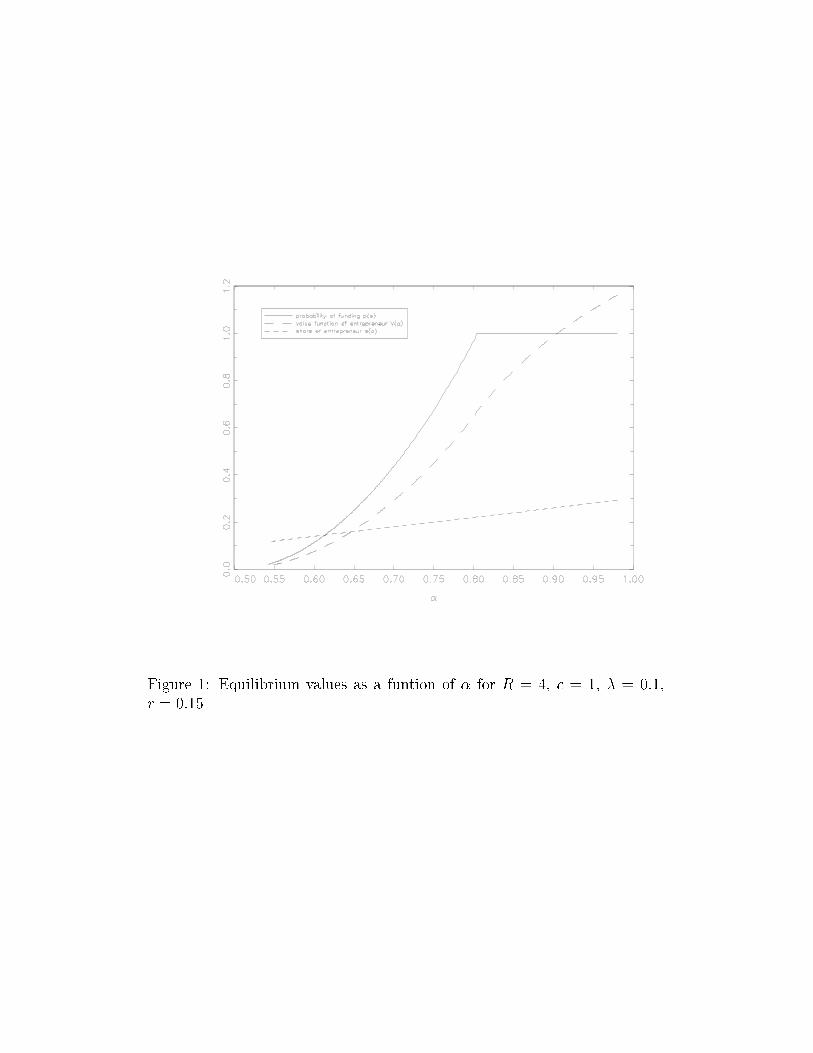
Figure 1: Equilibrium values as a funtion of � for R = 4, c = 1, � = 0:1,
r = 0:15

Figure 2: Symmetric information equilibrium values as a function of � for
R = 4, c = 1, � = 0:1, r = 0:15
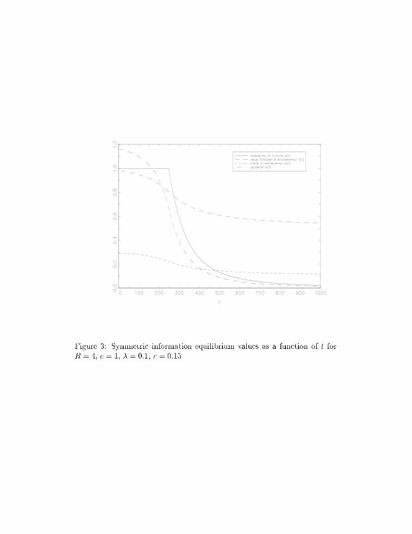
Figure 3: Symmetric information equilibrium values as a function of t for
R = 4, c = 1, � = 0:1, r = 0:15
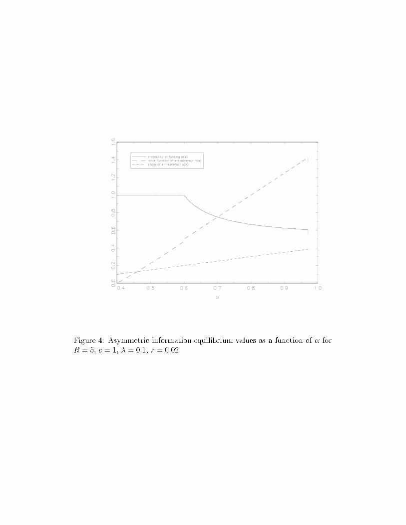
Figure 4: Asymmetric information equilibrium values as a function of � for
R = 5, c = 1, � = 0:1, r = 0:02

Figure 5: Asymmetric information quilibrium values as a function of t for
R = 5, c = 1, � = 0:1, r = 0:02

2
2
6
4
1 3 4
rccR λ+= 2
rλ
cR 4=
R
Figure 6: Evolution of funding probabilities p(α) in the ( rλ , R ) coordinates
for c = 1.