The financial instability hypothesis: A stochastic microfoundation framework

Contents lists available at ScienceDirect

Journal of Economic Dynamics & Control

Journal of Economic Dynamics & Control 35 (2011) 1151–1171

0165-18

doi:10.1

$ Fin

Technol

anonym� Cor

E-m1 Se

journal homepage: www.elsevier.com/locate/jedc

The financial instability hypothesis: A stochasticmicrofoundation framework$

Carl Chiarella, Corrado Di Guilmi �

School of Finance and Economics, The University of Technology, Sydney, PO Box 123, Broadway, NSW 2007, Australia

a r t i c l e i n f o

Article history:

Received 19 March 2010

Accepted 10 February 2011Available online 24 February 2011

JEL classification:

E12

E22

E44

Keywords:

Financial fragility

Complex dynamics

Stochastic aggregation

89/$ - see front matter & 2011 Elsevier B.V. A

016/j.jedc.2011.02.005

ancial support from the Paul Woolley Centre

ogy, Sydney is gratefully acknowledged. The a

ous referee for helpful comments and discus

responding author. Tel.: +61 2 9514 4746; fa

ail address: [email protected] (C. D

e the working paper series of the Levy Econo

a b s t r a c t

This paper examines the dynamics of financial distress and in particular the mechanism

of transmission of shocks from the financial sector to the real economy. The analysis is

performed by representing the linkages between microeconomic financial variables and

the aggregate performance of the economy by means of a microfounded model with

firms that have heterogeneous capital structures. The model is solved both numerically

and analytically, by means of a stochastic approximation that is able to replicate quite

well the numerical solution. These methodologies, by overcoming the restrictions

imposed by the traditional microfounded approach, enable us to provide some insights

into the stabilization policies which may be effective in a financially fragile system.

& 2011 Elsevier B.V. All rights reserved.

1. Introduction

Minsky (1977) defines financial fragility as ‘‘. . .an attribute of the financial system. In a fragile financial system continued

normal functioning can be disrupted by some not unusual event’’. The two key points highlighted by this definition are the‘‘not unusual event’’ that may stop the normal functioning of a financial system and that the system in question mustdisplay a certain degree of fragility. As regards the former point, there is no shortage of interpretations in this sense of thecrises that, at progressively shorter intervals, have hit capitalist economies (Kindleberger, 2005). The idea of an intrinsicinstability of the capitalist financial system dates back to Minsky (1982) and has gained increasing attention, especiallyduring the recent financial crisis.1 As regards to the second point, the identification of the degree of systemic fragility,according to Minsky, involves a microlevel analysis, as it depends on the ratio of financially sound to financially distressedfirms in the economy. More precisely, in his famous 1963 essay, Minsky classifies firms into hedge, speculative or Ponzitype. The first are the sound firms that can repay their debt and the interest on it. The second type are the ones able tomeet only the interest due on outstanding debt while, for the Ponzi firms, their cash flow is insufficient to fulfil neither therepayment of capital nor the interest due on outstanding debts.

As Taylor and O’Connell (1985) point out ‘‘Shifts of firms among classes as the economy evolves in historical time underlie

much of its cyclical behaviour. This detail is rich and illuminating but beyond the reach of mere algebra. What can perhaps be

ll rights reserved.

for Capital Market Dysfunctionality and the School of Finance and Economics at The University of

uthors would like to thank Masanao Aoki, Paul De Grauwe, David Goldbaum, Sherrill Shaffer and an

sions and Jonathan Randall for the excellent research assistance.

x: +61 2 9514 7722.

i Guilmi).

mics Institute of Bard College: http://www.levy.org/vtype.aspx?doctype=13.

www.elsevier.com/locate/jedc

dx.doi.org/10.1016/j.jedc.2011.02.005

mailto:[email protected]

http://www.levy.org/vtype.aspx?doctype=13

dx.doi.org/10.1016/j.jedc.2011.02.005

dx.doi.org/10.1016/j.jedc.2011.02.005

C. Chiarella, C. Di Guilmi / Journal of Economic Dynamics & Control 35 (2011) 1151–11711152

formalized are purely macroeconomic aspects of Minsky’s theories’’. According to them, this lack of formalism is one of thereasons for which Minksy’s work has been so far largely neglected.

Such is no longer the case. In recent years a consistent stream of research has started to deal with the microfoundationsof macroeconomics with heterogeneous and evolving agents. Significant results in terms of replication of empiricalstylized facts have been attained through the numerical solution of agent based models.2 From an analytical perspective,the most relevant contribution has been provided by Aoki,3 whose framework seems to allow a comprehensive analyticaldevelopment of Minsky’s theory that satisfactorily encompasses its essential microeconomic foundation.

Aoki adopts analytical tools originally developed in statistical mechanics. In his view, as the economy is populated by avery large number of dissimilar agents, we cannot know which agent is in which condition at a given time and whether anagent will change its condition, but we can know the present probability of a given state of the world. This approach hencefocuses in particular on the evolution of agents’ characteristics through time. The basic idea consists in introducing ameso-level of aggregation, obtained by grouping the agents into clusters according to a measurable variable. The dynamicsof the number of firms in each cluster defines as well the evolution of the whole economy, which is identifiable byspecifying some general assumptions on the stochastic evolution of these quantities. For example, assuming the dynamicsof occupation numbers to be a Markov process, it is possible to describe their stochastic evolution using the masterequation, which is a standard tool developed in statistical mechanics to model the evolution of ensembles of particles.Interaction among agents is modelled by means of the mean-field approximation (Aoki, 1996) that, basically, consists inreducing the vector of observations of a variable over a population to a single value. The usefulness and potential of thisapproach for analysing Minsky’s theoretical structure appears to be promising.

The aim of this paper is to propose a financial fragility model, along the lines of Minsky (1975) and Taylor and O’Connell(1985), with heterogeneous and interacting firms, using first a numerical simulation of the agent based model and thencomparing this solution with the one obtained by means of the stochastic dynamic aggregation technique mentionedabove. Besides the technical contribution, such a framework allows a deeper insight into the mechanism by which shocksare transmitted from the financial sector to the real economy. This aspect, which is central in Minsky’s approach, is not themain focus of Taylor and O’Connell (1985).

Our contribution concerns three main modifications that we bring to this original framework. The most relevant is themicrofoundation of the financial fragility approach. As already stressed, the presence of heterogeneous agents and theconsequent issues in consistently microfounding the framework are among the factors that have limited the diffusion ofMinsky’s approach through the economics profession. Here, differently from the original models, the equations areexpressed with reference to the microlevel composed of heterogeneous firms. We then study the macrodynamics usingtwo different approaches: the first being an agent based one, with the highest degree of heterogeneity, and the secondbeing a stochastic approximation, obtained by means of Aoki’s aggregation tools. The analytical solution complements theanalysis, allowing further insights into the model dynamics, very much in line with the approach proposed in Alfaranoet al. (2008).

The second modification derives from the observation that, from our perspective, the evaluation of capital assets comesfrom the stock market, in which investors display heterogeneous expectations about firms’ future profits. Thus we linkthese expectations to the dominant strategy in the stock market.

The third novel aspect regards the modelling of endogenous money which, if considered, is not analytically defined inthe cited studies. In the present treatment it is linked to the overall amount of financial assets rather than being a multipleof the monetary base as typically presented in the literature.4 In our opinion this view is more consistent with Minsky’sidea from two different perspectives. First, from a formal point of view, Minsky, in particular in his later writings,5 seemsto connect the degree of liquidity of the system to a wider range of marketable paper, such as for example, securities andderivatives, than the typical monetary aggregates. As a consequence financial innovation, besides having the effect oftransferring risk, also influences the credit supply by affecting the endogenous determination of the degree of liquidity inthe economy. Second, from a theoretical point of view, by modelling endogenous money as endogenous wealth, theavailability of credit is linked to the conditions of the financial system and, in particular, to the expectations of investors,providing a quantitative benchmark for the analytical representation of his idea of increased propensity to supply credit inperiods of expansions (Minsky, 1963). In this way we define a mechanism of endogenous credit creation, a concept largelyneglected by the literature.6

The outline of the paper is as follows. The next section introduces the previous models in order to define the generalcontext of the present contribution. Section 3 describes the general features of the model and outlines the basic structureof firms in the agent based framework. The behavioural hypotheses and equations are the same for the agent based set upand for the stochastic approximation; in the former they refer to each single firm, without limitation on the degree ofendogenous heterogeneity, while the stochastic dynamics considers a representative firm for each category. Section 4defines the hypotheses concerning investors and the capital market. Section 5 discusses the stochastic approximation to a

2 See by way of example Axtell et al. (1996) and Delli Gatti et al. (2005b).3 Namely, Aoki (1996, 2002) and Aoki and Yoshikawa (2006), with a further development provided by Di Guilmi (2008).4 For a review see Fontana (2003).5 As in Minsky (2008) about debt securities.6 Exceptions are Jarsulic (1989) and Keen (1995).

C. Chiarella, C. Di Guilmi / Journal of Economic Dynamics & Control 35 (2011) 1151–1171 1153

high order heterogeneous model. Section 6 presents the outcomes of the simulations for the agent based model andcontrasts them with the stochastic approximation results. Section 7 concludes with some discussion of the questions thatcan be addressed using the framework developed here.

2. The general framework

Minsky presented his theory of investment in chapter 5 of his 1975 book John Maynard Keynes. He refers to a genericproductive unit, for which the expectations about future returns on investment are quantified by a variable Pk. It is givenby Pk,t ¼ CtðKtÞ, where C is the capitalization factor and K the amount of all the existing assets at time t. Unlike Tobin(1969), this capitalization price may differ from the current price P of new capital, due to less than perfect foresight. Thedecision of the firm about its investment is based on this difference, and it can lead the firms to invest beyond theavailability of their cash flow and therefore to borrow external funds. Thus the capitalization price is impacted by theleverage level of the firm and, more precisely, by the evaluation of risk by both borrower and lender. As noted by Keynes inthe General Theory, cited by Minsky (1975): ‘‘During a boom the popular estimation of the magnitude of both these risks,both borrower’s risk and lender’s risk, is apt to become unusually and imprudently low’’, consequently raising thewillingness to invest.

On the financial side, the market valuation of the shares of a firm may differ from the present value of its capital, withthe difference being absorbed by net worth. Given the substitutability of assets, a shift of investor preferences impacts onthe net worth of firms via a different evaluation of capital assets.

Therefore, investor expectations of future profits influence, on the one hand the prices of firms’ equities on the stockmarket and, on the other hand the current value of firms’ assets. For example, if the market forecasts a rise in the demandfor a certain product, there will be an increase in the evaluation of the machines that produce that good and acontemporaneous rise in the price of shares for the firms that sell them (Wray and Tymoigne, 2008). These two effectsshape firms’ decisions on investment and, as a consequence, output and employment levels. At the aggregate level then theeconomy may experience periods of growth, depression or fluctuations due solely to changes in the market mood and notto its actual productivity.

Taylor and O’Connell (1985) developed this framework proposing an aggregative model with a real and a financialsector. For what concerns the real sector, they set up a functional relationship between Pk, the current level of the interestrate and the present and prospective return on investment, according to

Pk ¼ ðrþrÞP=i, ð1Þ

where r is the current profit rate and i the interest rate. The key variable in their study is r which represents the differencebetween the expected return on capital and its present value r. In the financial part of the model, investors allocate theirwealth among liquid assets, equities issued by the firms and government bonds. The share of wealth invested in eachactivity is calculated by means of a system of equations whose arguments are the interest rate and the current andexpected rate of profit of firms. Therefore, the key variable in the framework is the expected profitability r whichrepresents the connection between the financial and the real sectors. In their model it is left exogenous and investors areassumed to take into consideration the fundamentals of productive firms.

As anticipated we use the same theoretical structure but frame it in a bottom-up approach with heterogeneous firms,each having a different expected profitability. Also, we propose a way to endogenise r, defining it as a function of thestrategies in the stock market. More precisely we assume that each r is a function of the proportion of investors adopting afundamentalist or chartist strategy with an idiosyncratic multiplicative shock. According to the value of r investors pricefirms’ equities and allocate their wealth among equities, firms’ bonds and liquid assets. In the real sector, firms calculatetheir Pk according to Eq. (1) and decide on the level of investment. Therefore, the heterogeneity of r implies heterogeneityin firms’ investment levels and, as a consequence, in size and in their need of external financial resources.

3. Firms

This section presents the structure of the agent based model. Variables are written with the superscript j when theyrefer to a generic firm, while the mean-field values, that are introduced in Section 4, are identified by the subscript z¼ 1,2.Aggregate variables appear without any sub- or superscript. The model is set up in continuous time. The hypotheses arelisted below:

�
Due to informational imperfections on capital markets (Myers and Majluf, 1984), firms prefer to finance theirinvestments Ij with retained profits Fj and, only if these are not sufficient, by the emission of new equities Ej or withnew debt Dj. � Firms are classified into two groups, clustering together the speculative and Ponzi firms of the Minsky (1963)
taxonomy. In order to ease the calculations, analogously to Lima and Meirelles (2007), the threshold level of debt is setto 0. Therefore, the classification defines as speculative (type 1) the firms that have to finance their investment withdebt or new equity and as hedge (type 2) the firms that can finance all their investments with retained profits. Thus


firms can be classified into two states, depending on whether or not they display a positive debt in their balance sheet:3 state z=1: DjðtÞ40,3 state z=2: DjðtÞ ¼ 0.

This classification is the basis for the analytical solution of the model that is detailed in Section 5 below.
� Every period the j-th firm targets an amount of investment Ij. The new level of capital then determines the demand for
labour and the output. The investment is decided on the base of the shadow price of capital Pjk which has the same

meaning as in the cited works, so that

IjðtÞ ¼ aPjkðtÞ, ð2Þ

where a is a parameter measuring the sensitivity of firms to the current value of capital assets and the shadow price Pk

is specified below. This formulation recalls the one adopted by Delli Gatti et al. (1999), while the model of Taylor andO’Connell (1985), very much in line with Minsky (1975), takes into account the price differential between the shadowprice and the price of furnishing new investment goods. Our choice in (2) is motivated by the fact that the solutionadopted by Taylor and O’Connell (1985) would add a factor that might turn out to be too noisy for the identification ofthe effects of financial market fluctuations on investment.In the present treatment, Pj

k is determined according to

PjkðtÞ ¼

rjðtÞPðtÞ

iðtÞ, ð3Þ

where i is the interest rate. As highlighted with reference to (1), in the study of Taylor and O’Connell (1985) r is definedas the difference between the expected rate of profit and the present rate r. Here we do not make such a distinction andsimply consider rj as the expected rate of profit for firm j. For each firm, the accumulation of capital is given by theinvestment Ij(t) less the depreciation of the existing capital stock, measured by the constant rate v.
� Firms produce a good that can be used either for consumption or investment. The selling price of the final good is
obtained by applying a mark-up t on the direct production costs according to

PðtÞ ¼ ð1þtÞwðtÞb, ð4Þ

where w is the nominal wage and b is the labour-output ratio. The parameters t and b are assumed to be constant whilethe variable w is defined below. These quantities are equal for all firms.
� All salaries are consumed and the unit salary varies in each period in order to ensure the equilibrium in the product
market. In particular it is equal to

wðtÞ ¼IðtÞ

tbXðtÞ, ð5Þ

where X(t) is the total output.
� Assuming that the firms adopt a technology with constant coefficients, the amount of labour requested is residually
determined once the optimal level of investment, and hence of capital, is quantified. The supply of labour is infinitelyelastic. The production function G for firm j is written as

XjðtÞ ¼ GðKjðtÞ,LjðtÞÞ ð6Þ

with K and L representing, respectively, physical capital and labour. Given that the supply of labour is infinitely elastic andthe output/labour ratio b is constant, it is possible to define the production function just as a function of capital so that

XjðtÞ ¼j KjðtÞ, ð7Þ

where the output/capital ratio j is a constant parameter.
� Firms finance the part of investment that cannot be covered with internal funds by a fraction f iðtÞ of equities, where f40
is a parameter, and then the rest with debt, the dependence on the interest rate reflecting the fact that in periods with ahigh interest rate equities would be preferred. The price of the new capital goods is assumed to be equal to the final goodsprice P. The sum of retained profits is indicated by Fj. Thus, the variations of Ej and Dj at an instant of time are given by

dEjðtÞ ¼f iðtÞ

PðtÞIjðtÞ�FjðtÞ

Pe1ðtÞ

� �dt, ð8Þ

dDjðtÞ ¼ ½1�f iðtÞ�½PðtÞIjðtÞ�FjðtÞ� dt ð9Þ

where Pe1 is the price of equities for speculative firms to be defined in the following section.
� The timeline of the whole process over successive time intervals is shown in Fig. 1. In the first stage market
expectations determine the shadow price of capital and the desired level of investment. In the following unit of timefirms implement the decision, modifying the capital stock and producing the final good. The product is then sold in thesubsequent period, giving rise to a profit (or loss).

Fig. 1. Timeline of the investment process.


�

resp

Profits are given by

pjðtÞ ¼ PðtÞXjðtÞ�wðtÞbXjðtÞ�iðtÞDjðtÞ ¼ twðtÞbXj

ðtÞ�iðtÞDjðtÞ: ð10Þ

Accordingly, the variation in retained profits, or cash flow, for a hedge firm is

dFjðtÞ ¼ ½pjðtÞ�PðtÞIjðtÞ� dt: ð11Þ

If, at time t, FjðtÞoPðtÞIjðtÞ, the firm becomes speculative and Ij(t)�Fj(t) will be financed with new equities and debtaccording to Eqs. (8) and (9).
� A firm fails if its debt level exceeds some multiple of its capital stock, that is if
DjðtÞ4cKjðtÞ ð12Þ

with c41. The probability of a new firm entering is directly proportional to the variation in the aggregate productionwith respect to the previous period.

4. Investors

Even though a comprehensive modelling of stock markets would go beyond the aim of the present analysis, somebehavioural assumptions on investors are needed for the internal consistency of the framework. This section illustrates thehypotheses and the conditions of equilibrium for the capital market.

4.1. Behavioural hypotheses

Investor preferences are modelled in a Keynesian fashion, assuming that a share of wealth is kept liquid. Minsky (1975)gives to the usual Keynesian motives for holding money (transaction, precautionary, speculative) a formal representation,modelling the demand for liquid assets as a function of income, interest rate, asset price, firm debt and near money supply. Wemodel the demand for liquid assets in a similar way. Moreover, we assume that the financial operators act according to abounded rationality paradigm. Consequently, in order to quantify the level of confidence of the market in each period,we classify investors into two broad categories of chartists and fundamentalists, within an approach that has an establishedtradition in the literature.7 It has been demonstrated (Aoki and Yoshikawa, 2006, Chapter 9) that this classification accounts foralmost the totality of different possible strategies. We adopt this assumption, which turns out to be particularly suitable in thisframework. Indeed we can reasonably assume that, on average, fundamentalists, focusing on the real value of firms, will favourinvestment in hedge firms, while chartists, who base their decisions on extra-balance sheet information, may prefer riskierequities.8 We assume that all investors maximize a CARA utility function in order to avoid the distinction between chartist andfundamentalist wealth. Since our focus is on how changes in investor expectations impact on the real economy, we assume thatvariations in the proportion of the types of operators are not dependent on firms’ performance and are simply governed by astochastic law. This also allows for a wider range of possible outcomes and behaviours as a result of the multiplicity ofexogenous factors (not related to the economy) that influence the markets.

4.2. The determination of r

As anticipated, the variable r plays a key role in the entire story, as it incorporates expectations that emerge in financialmarkets into the decision process of firms about investment. Taylor and O’Connell (1985) introduce it in order to betterisolate the effect of the difference between the anticipated return and the current profit rate, an effect that in the originaltreatment of Minsky (1975) is directly incorporated in the shadow price Pk. As Taylor and O’Connell (1985) were notinterested in the impact of financial markets they did not explicitly model r, assuming independence between thebehaviour of investors and firms. In contrast since our perspective is mainly focused on the transmission of shocks fromthe financial sector, the role of r is reminiscent of Tobin’s q (Tobin, 1969), in that it is connected to equity values. In thissense our work constitutes a bridge between these two approaches and indeed is an extension of them.

7 See for example Zeeman (1974), Lux (1995), Brock and Hommes (1997), Chiarella and He (2003) and Chiarella et al. (2009).8 We adopt here a broader definition of chartist strategy than the standard used in the literature. We refer to it as a generic alternative approach with

ect to the fundamentalists rather than purely as a pricing rule inferred by analysis of time series of past prices.


Two basic assumptions are at the root of the formulation of r: the first is its dependence on the relative proportion ofchartists and fundamentalists in the market; the second concerns the formation of expectations. As anticipated, sincefundamentalists look at the balance sheet of firms while chartists use other information and focus only on the evolution ofreturns, we can assume that an increase in the proportion of chartists heightens the expectations about indebted firms that, onthe contrary, reduce when the share of fundamentalists is bigger.9 Accordingly, rj is determined differently depending onwhether a firm is in state 1 or in state 2 as a direct or indirect function of the proportion of chartists nc, namely

rj1 ¼ f1ðn

cÞ ¼ nc ~$ j,

rj2 ¼ f2ðn

cÞ ¼ ð1�ncÞ ~$j, ð13Þ

where ~$j is an idiosyncratic random variable specified over a constant positive support and E½$� ¼ 1. As one can see,at each time the value of r for each firm is the result of two independent random shocks: the proportion of chartists nc in themarket at that time, which is common for all firms, and the variable ~$ j which is different for each unit. Thus on average abigger fraction of chartists in the market leads firms in state 1 to increase their investments, their production and their debt. Atthe same time, the growing demand for credit puts pressure on interest rates. Therefore, the system experiences a debt drivenexpansion that makes it progressively more vulnerable to sudden changes in investor expectations.10

4.3. Equilibrium in the capital market

The equities of the two different types of firms can be correspondingly sorted into two classes with different associatedrisks.11 Investors will allocate part of their wealth between the two classes of shares according to the market expectationat the time of choice. In order to make the pricing model analytically tractable, we follow the mean-field approachdiscussed in the introduction and replace all the interactions among the heterogeneous firms and the investors with anaverage interaction. Namely we make use of the two indicative values r1 and r2, calculated as a statistic of the rj withineach cluster of firms, which represent the benchmark values for investors in order to allocate their wealth and price thetwo types of shares.

The wealth W of investors is the sum of shares, bonds and liquid assets, so that

WðtÞ ¼ Pe1ðtÞE1ðtÞþPe2ðtÞE2ðtÞþDðtÞþMðtÞ, ð14Þ

where M(t) is the nominal demand for liquid assets, E1(t) and E2(t) are the quantities of shares of, respectively, speculativeand hedge firms in the market, while Pe1(t) and Pe2(t) are their prices. Wealth evolves over time according to

dW

dt¼

dPe1

dtE1ðtÞþ

dPe2

dtE2ðtÞþPe1

dE1

dtþPe2

dE2

dtþ

dD

dtþ

dM

dt: ð15Þ

An initial endowment of money is assumed. Variations in total wealth are then due to capital gains, which in thisframework constitute high-powered wealth.

Investors allocate their wealth among equities, firm bonds and liquid assets according to the proportions:e1ði,r1,r2,cÞ,e2ði,r1,r2,cÞ, bði,r1,r2,cÞ and Cði,r1,r2,cÞ that satisfy the constraint e1þe2þbþC¼ 1. The parameter creflects the propensity toward liquid assets and it is assumed to be constant over time. Given the structure of the equilibriumconditions, and in particular the fact that the demand for credit is always (partially) accommodated, the bigger is c the largerare M and the aggregate wealth W. Thus, this parameter may be interpreted as a proxy for the capacity of the system togenerate endogenous credit. The proportions of the two kinds of strategies influence r and through this the allocation of wealthbetween the different assets. The equilibrium conditions on equities and credit markets are (time indices are omitted)

e1ði,r1,r2,cÞPe,1

W ¼ E1,

e2ði,r1,r2,cÞPe,2

W ¼ E2,

bði,r1,r2,cÞW ¼D,

Cði,r1,r2,cÞW ¼M,

W ¼ Pe1E1þPe2E2þDþM:

8>>>>>>>>>>><>>>>>>>>>>>:

ð16Þ

The system (16) may be solved for the value of asset prices, interest rate, demand for money and aggregate rentiers’ wealth.This latter turns out to be endogenously determined within the system in order to (partially) accommodate the demand forcredit.

9 In this sense the proportion of chartists can be regarded as a quantification of the market euphoria as described by Minsky.10 Our aim is to study how the economy reacts to unpredictable and possibly contradictory external shocks, without setting up an ad hoc circular

feedback between expectations and aggregate output. Hence we do not propose an explicit formulation for the return on equity, which would imply, to

some extent, an explicit modelling of expectations as a function of the performance of the macroeconomy.11 Actually, in each period, only speculative firms issue equities, given that hedge firms can finance all their investment with retained profits. In any

event in the market there are also the equities of firms that were speculative and became hedge, which would be assessed differently by investors.


5. Stochastic dynamics

In this section we apply the stochastic aggregation method that we introduced and briefly described in Section 1 to themodel described above. We have already set up a suitable structure classifying firms into two groups. Now we aim todescribe the evolution of the whole system by quantifying the dynamics of the proportions of firms in the two clusters.Two additional hypotheses are needed in order to develop the analytical solution: first, that firms switch from one state toanother according to a jump Markov process; second, that the number of firms N remains constant.

The first stage for this analytical treatment is the definition of the probability for a firm to switch from one group to theother (the transition probability). It would be analytically not feasible to quantify this probability for each firm in thesystem. Thus, a preliminary step is to define an average or representative firm for each cluster by means of the mean-fieldapproach. Our discussion so far has been in terms of single firms, referring all the variables to the agent level, and only inthe last section we have introduced the mean-field approximations rz, z¼ 1,2. These variables allow us to set up the toolsfor the analytical solution of the model. Eqs. (2) and (3) can be computed starting from the mean-field values rz in order tocalculate the variables Iz and then to identify, using the other equations of the agent based model, two firms that arerepresentative of each group. It is then possible to calculate the two transition probabilities (of entering and exiting a state)referring to these two firms. Multiplying these probabilities for the unconditional probability of being in one of the twostates we obtain the transition rates, which quantify the probabilities of observing a transition from one state to another ina unit of time. Finally, the transition rates are used to set up the master equation in order to identify the stochasticevolution of the number of the two types of firms.

Therefore, the model is able to generate dynamics in two different ways: an agent based approach with N differentagents and a stochastic approximation, with two different firms: one ‘‘good’’ and one ‘‘stressed’’.

5.1. Transition probabilities

The probability for a firm to transition from state 2 to state 1 depends upon its desired level of investment and retainedprofits, so a hedge firm becomes speculative if the former is bigger than the latter. Therefore, the probability z for a firm tomove from states 2 to 1 is equal to

zðtÞ ¼ Pr½PðtÞ I2ðtÞZF2ðtÞ�

¼ Pr ar2ðtÞPðtÞ

iðtÞZF2ðtÞ

� �, ð17Þ

where to obtain the second expression we make use of Eqs. (2) and (3).With regard to speculative firms, they can move to state 2 if they are able to generate a level of profit sufficient to repay

their debt; so that the relative probability of transition n is given by

nðtÞ ¼ Pr½twðtÞbX1ðtÞZD1ðtÞð1þ iðtÞÞ�

¼ PrftwðtÞbG½K1ðtÞ,L1ðtÞ�ZD1ðtÞð1þ iðtÞÞg

¼ Pr twðtÞbG K1ðt�dtÞþar1ðtÞPðtÞ

iðtÞ,L1ðtÞ

� �ZD1ðtÞð1þ iðtÞÞ

� �, ð18Þ

where to write the second equation we have used Eq. (6) and for the third we refer to Fig. 1. Substituting (13) into (17) and(18) and considering that E½$� ¼ 1 we can express the transition probabilities in terms of the known probability functionof nc, so that

zðtÞ ¼ FðnczÞ ¼ Pr ncðtÞr2�

F2ðtÞiðtÞ

PðtÞa

� �: ð19Þ

nðtÞ ¼ 1�FðncnÞ ¼ Pr ncðtÞ4

iðtÞ

PðtÞ a

D1ðtÞð1þ iÞ

twðtÞbj �K1ðt�dtÞ

� �� : ð20Þ

The expressions on the right hand sides are the critical levels in the proportion of chartists ncz and nc

n required for a firm toshift from one group to the other.

In order to quantify the transition rates, let us denote with Z the a-priori probability for a firm to be in state 1, taking itas exogenous.12 The transition rates will be then given by

lðtÞ ¼ ð1�ZÞzðtÞ,

mðtÞ ¼ ZnðtÞ:

12 As demonstrated in Aoki (2002) the solution of the master equation also provides a possible endogenous formulation for the probability Z. We do

not apply this result here as it is not essential in the present study.


5.2. The system dynamics

We have already defined the microstates of the process that correspond to states 1 and 2 for the firms. In order to definethe macrodynamics we focus on the occupation numbers, that is the number of firms which are in one of the states at agiven time. These occupation numbers identify the macrostates of the process, which accordingly, are given by all thepossible combinations of N1 and N2 satisfying the constraint N1þN2 ¼N. In this way, their stochastic dynamics can beconveniently described by a master equation (Kubo et al., 1978; Aoki, 2002). Using Nz to denote the occupation number forthe state z, the master equation can be expressed as

dPrðNz,tÞ

dt¼ lPrðNz�1,tÞþmPrðNzþ1,tÞ�ðlþmÞPrðNz,tÞ, ð21Þ

where Pr(Nz,t) indicates the probability of observing an occupation number equal to Nz in state z at time t. This ordinarydifferential-difference equation for Pr(Nz,t) allows us to describe the stochastic dynamics of the occupation numbers byidentifying the components of the stochastic process that governs their evolution. To this end Aoki (2002) suggestssplitting the state variable Nz into its drift (m) and diffusion (s) components, according to

NzðtÞ ¼NmþffiffiffiffiNp

s: ð22Þ

At this stage it is possible to apply the method detailed in Di Guilmi (2008) and Landini and Uberti (2008) to obtain thedynamics for m and s. The calculations detailed in the Appendix demonstrate that the asymptotic solution can berepresented by the system of coupled equations13

dm

dt ¼ lm�ðlþmÞm2, ð23Þ

@Q ðs,tÞ@t

¼ ½2ðlþmÞm�l� @@sðsQ ðs,tÞÞþ ½lmð1�mÞþmm2�

2

@

@s

� �2

Q ðs,tÞ, ð24Þ

where the first is an ordinary differential equation the solution of which is the drift of the process Nz, while the partialdifferential equation (24) describes the evolution of the density of the random spread s around the drift. As one can seefrom (23), m converges to the steady state value mn given by

m� ¼l

lþm: ð25Þ

Eq. (23) describes the evolution of the fraction m of firms and we see that it is fully dependent on transition rates.The solution of the equation for the density of the spread component, as shown in the Appendix, yields the limitdistribution function Q ðsÞ ¼ limt-1Q ðs,tÞ for the spread s, determining, in this way, the long run probability distribution offluctuations, namely

Q ðsÞ ¼ Cexp �s2

2s2

� �, ð26Þ

where s2 ¼ lm=ðlþmÞ2. Eq. (26) is a Gaussian density whose parameters are dependent on the transition rates.

5.3. Analytical description of the model

At this point we are able to identify the two dynamical variables that drive the dynamics of the economy: the first iscapital accumulation that reflects investors’ expectations and animal spirits, and the second is the underlying stochasticdynamics of the proportion of speculative firms. These two dynamical variables are connected via the fact that thetransition rate l is a function of the level of investment I2 and the aggregate investment depends on the shares of the twotypes of firms. Taking as state variable the share of speculative firms n1 ¼N1=N whose average trend is given by Eq. (23),we have

dn1ðtÞ ¼ fln1ðtÞ�ðlþmÞ½n1ðtÞ�2g dtþs dW ,

dKðtÞ ¼ IðtÞ dt�vKðt�dtÞ

¼ Nf½aPk1ðtÞ�n1ðtÞþ½aPk2ðtÞ�½1�n1ðtÞ�g dt�vKðt�dtÞ,

8><>: ð27Þ

where dW is a stationary Wiener increment and s dW is the stochastic fluctuation component in the proportion ofspeculative firms, coming from the distribution (26). These dynamics can then also identify the evolution of employmentand aggregate output.

13 As illustrated by Eq. (A.17) in the Appendix, t is the time rescaled by the factor N.


In order to highlight the role of the proportions of two types of investors and firms we substitute Eqs. (3) and (13) intothe second equation in (27) and considering that E½ ~$� ¼ 1, we can write the investment term as

IðtÞ ¼NaPðtÞ

iðtÞ½n2ðtÞþn1ðtÞð2ncðtÞ�1Þ�: ð28Þ

Eq. (28) sheds light on the dynamics of the agent based model and, in particular, it analytically represents the factthat the effect of the proportion of the number of speculative firms depends on market expectations. As long as the speculativefirms are the majority, a proportion of chartists nc 40:5 causes a positive variation in investment due to the expected rise in theasset price combined with the high market valuation of their equities. When expectations change and the fundamentalistinvestors prevail, the proportion of speculative firms has a negative effect on investment.

Fig. 2 presents some results from the simulations providing some further insight into the dynamics. For a proportion ofchartist lower than 0:5, there is an inverse relationship with the interest rate (as shown in the upper panel of the picture) and adirect relationship with the proportion of speculative firms in the following period (lower panel in the same figure) and the

Fig. 2. Scatter plots of the proportion of chartists and interest rate (upper panel) and lagged variation in the proportion of speculative firms (lower panel).

Based on the simulation of the agent based model.

Fig. 3. Flowchart of the model. Time indices are omitted.


accumulation of capital. This may be due to a liquidity effect in the right part of the graph (investors own an increasing quantityof bonds and then there is a positive liquidity effect) that pushes firms to increase their leverage. On the contrary, when thechartists become the majority the system is placed under pressure, determining a higher interest rate, because of the largerdemand for credit. In the following period the failures of speculative firms will shrink both their proportion and the aggregatecapital. This nonlinear mechanism is a possible cause of the emergence of right-skewed distributions at the aggregate level, asshown in the simulations in the following section, even with Gaussian fluctuations at the microlevel.

The different steps through which the model works are illustrated by the flow chart in Fig. 3. The chart highlights thefact that the key variable in the entire story is r. Thus the entire dynamics start with the calculation of this variable foreach unit in the system (first box on the left). Then these values impact, on the one hand, the financial sector and, on theother hand, the real sector. The two parts of economy are represented on the two sides of the chart. The left partsummarizes the stages through which it influences the equilibrium prices in the financial market. Investors assessdifferently the shares of the two types of firms, so they refer to the mean-field values r1 and r2, computed from the rj

z

within each cluster z of firms. These two variables, together with the parameter c, are the inputs into the system whichyield simultaneously the prices of the two shares, the interest rate and the demand for liquid assets. The right side of thechart details the determination of the amount of new investment for each firm through the different stages. Aftercomputing the value r and Pk, the level of investment is quantified for each firm. The amount of new investment, summedto the existing capital, quantifies the production and, then, the profits. The difference between the amount of retainedprofits less the cost of the new investment eventually determines the state (speculative or hedge) of each firm. As shownby the box at the bottom in the middle, the dynamics of aggregate capital can be therefore described by both the evolutionof capital priced at Pk and the amount of financial assets in the economy.

6. Simulations

This section presents the general settings of the simulations and their results. First (in Subsection 6.1) we present thefunctional forms and initial conditions. In Subsection 6.2, the results are illustrated and discussed, with particularattention paid to the possible analytical explanations for the aggregate outcomes and some suggestions for an adequateeconomic policy in a financial fragility context.

6.1. Specification of functional forms

The functions e1, e2, b and C of the system (16) are formulated as logistic functions, in order to ensure meaningfulvalues of the proportions of wealth invested in the different activities. The shares of wealth invested in hedge firm equities,speculative firm equities, debt and money are assumed to be positively related to, respectively, r2, r1, the rate of interest i

and the parameter c. The shares are thus given by

e1ðtÞ ¼1

1þeiðtÞþr2ðtÞþc�r1ðtÞ, ð29Þ

e2ðtÞ ¼1

1þeiðtÞþr1ðtÞþc�r2ðtÞ, ð30Þ

bðtÞ ¼1

1þer1ðtÞþr2ðtÞþc�iðtÞ, ð31Þ

CðtÞ ¼1

1þeiðtÞþr1ðtÞþr2ðtÞ�c: ð32Þ

The parameter c is kept fixed. Therefore the system (16) becomes

Pe1ðtÞE1ðtÞ ¼WðtÞ

1þeiðtÞþr2ðtÞþc�r1ðtÞ,

Pe2ðtÞE2ðtÞ ¼WðtÞ

1þeiðtÞþr1ðtÞþc�r2ðtÞ,

DðtÞ ¼WðtÞ

1þer1ðtÞþr2ðtÞþc�iðtÞ,

MðtÞ ¼WðtÞ

1þeiðtÞþr1ðtÞþr2ðtÞ�c,

WðtÞ ¼ Pe1ðtÞE1ðtÞþPe2ðtÞE2ðtÞþDðtÞþMðtÞ:

8>>>>>>>>>>>>>><>>>>>>>>>>>>>>:

ð33Þ

The mechanism for entry of new firms is stochastic. In every period a random number drawn from a uniform distributionwith support [0,1] is assigned to each potential new firm; if this number is bigger than the normalized variation ofaggregate output observed in the previous period the firm becomes active. The variation is normalized such that avariation of +12% is equal to 0 and of �12% is equal to 1. A typical configuration of parameters is: a=4; f¼ 1; c=7;c¼ 0:25; v¼ 0:009. A control is introduced in order to ensure that fir1. These parameters have been calibrated in order


to obtain the best performance in terms of replication of empirical data. The values of rz are the mean of the rj’s includedbetween the 10th and the 90th percentiles within each cluster of firms. As a starting condition, all firms are hedge, havingan initial endowment of internal funds, and the initial interest rate is set to 0.1.

The random variables nc and ~$ are assumed to have a uniform distribution with supports nc 2 ½0,1� and ~$ 2 ½0:01,1:99�.

6.2. Simulation results

Simulations are performed by implementing two separate procedures, one agent based and the other for the stochasticdynamics of Section 5, and each produces its own dynamics of proportions of firms and capital accumulation. The twoprocedures are linked as the exogenous shock of the variation in nc is the same for both and the mean-field variables rz,obtained from the rj of the agent based simulation, are the inputs for the stochastic approximation. Then, the routine forthe agent based model is replicated with the two representative firms for each state, obtaining dynamics driven by thestochastic system (27).

The transition probabilities are normalized by taking the theoretical maximum and minimum values of the right-handside of the inequalities in (19) and (20). We performed simulations for different numbers of periods and the results havebeen verified by running 1000 Monte Carlo replications for each simulation. A period can be considered as a year and theaverage interest rate for each replication is about 11%.

6.2.1. Distributional results and analytical insights

The model replicates well some quantitative features of US economy as far as the relationships of GDP dynamics withmarket capitalization and business debt are concerned. The results are displayed in Table 1.

The model is also able to replicate some statistical regularities that are observed in real data. The distribution ofvariations in the aggregate output is well approximated by a Weibull distribution (Fig. 4) as found by Di Guilmi et al.(2005) and the distribution of firms’ growth rates is well fitted by a double exponential PDF (Fig. 5 for profits) as detectedby Stanley et al. (1996). The size of speculative firms is distributed according to a Pareto law while the distribution ofhedge firms, on average larger and more dispersed, is well fitted by a lognormal one. The overall distribution of sizeappears therefore as a bimodal distribution (Fig. 6).

These regularities are connected as pointed out by the existing literature on firm size distribution. The appearance of alognormal distribution for surviving firms has been explained by Gallegati and Palestrini (2010). They show that it is theresult of the Kesten process of growth with lower bound. Here firms do not retire their capital and the maximum negativegrowth (for the hedge) is the rate of depreciation which therefore provides a lower bound. With regard to speculativefirms, they display, on average, larger rates of growth than the hedge ones. This is because during the boom periods theygrow faster while the growth of the hedge ones appears to be steady. This higher growth lasts until the turning point,when the weakest firms begin to fail, whilst the hedge units display a smoother evolution. This is confirmed by the debtdynamics, which during booms grows faster than capital, and by Figs. 6 and 7 which show, respectively, the firms sizedistributions during expansions and contractions and the shift of the hedge firms distribution to the right. Fig. 6 alsodisplays how the distribution of type-1 firms is more even during upturns, matching the empirical evidence presented byGaffeo et al. (2003) for the G-7 countries.

We can conclude that the positive long run trend is mainly given by the growth of the hedge firms while the periods ofboom and bust are mainly due to the dynamics of the speculative units. This fact is another possible explanation of theemergence of non-Gaussian outcomes at the aggregate level with Gaussian distributed fluctuations in the proportions ofthe two types of firms. Indeed, as evidenced by different papers (Gabaix, 2009; Delli Gatti et al., 2005a,b), right-skeweddistributions for macrofluctuations can be interpreted as the result of the underlying power law distribution of firms size.

6.2.2. Dynamics and policy indications

Fig. 8 reports the dynamics of the capital and the share of speculative firms. For both variables the stochasticapproximation mimics the results produced by the agent based simulation. The distribution of variations in n1 convergesto a normal which the bi-dimensional Kolmogorov–Smirnoff test confirms to be the same for the numerical and the

Table 1Results from Monte Carlo simulation of the model and comparable evidence for the US. Sources: market capitalization 1929–2008: CRSP data set; GDP

1880–2007: International Monetary Fund; business debt: Federal Reserve Bank of St. Louis. GDP fluctuations are calculated as variations on the long term

GDP trend.

Variable Empirical evidence Simulations

Correlation market cap.-GDP (1929–2000) 0.7000 0.6962

Mean market cap.-GDP ratio (1929–2000) 0.629470.3648 0.614170.2550

Correlation debt-GDP (1950–2007) 0.8612 0.8051

Mean debt-GDP ratio (1950–2007) 0.518170.1423 0.520870.1658

Variance in GDP fluctuations (percentage, 1950–2007) 0.0022 0.0022

Fig. 4. Frequency distribution of positive (upper panel) and negative (lower panel) variations in aggregate production with Weibull fit. Based on the

simulation of the agent based model.

Fig. 5. Frequency distribution of rates of variations in firms profits with Laplace fit. Based on the simulation of the agent based model.

Fig. 6. Pareto fit for speculative firms capital and lognormal fit for hedge firms capital during expansions and recessions. Based on the simulation of the

agent based model.


Fig. 7. Lognormal distribution fit of hedge firms capital at different time steps. Based on the simulation of the agent based model.

Fig. 8. Different dynamics of capital (upper panel) and share of speculative firms (lower panel). Simulation of the agent based model (continuous line)

and the endogenous stochastic approximation (dashed line).


analytical solutions. The distribution of variations in the aggregate output is well approximated by a Weibull distributionfor both solutions. Despite very close values for the parameters the test in this case rejects the null hypothesis that the twodistributions are identical.

The dynamics of capital (and consequently of aggregate production) displays a long term upward trend. Within thistrend, long cycles of a duration varying between about 10 and 30 periods and smaller variations (from one periodto another) are identifiable. The length and the amplitude of the cycles are determined by the underlying debt cycle(see Fig. 9). During periods of accelerated growth, the proportion of speculative firms and aggregate debt rise. Consistentlywith Minsky’s model, the growth and the accumulation of debt increase until the most indebted speculative firms begin tofail, reducing the amount of capital and the aggregate wealth in the system. The amount of available credit reduces,causing the demise of other speculative units. This downward spiral ceases when all the firms in the relatively worstfinancial condition have collapsed, allowing the cycle to start again. The dynamics of bankruptcies and capital arecompared in Fig. 10. These dynamics are interesting in particular because in the model there exists no feedback from thesector of firms to the financial market. Indeed, market sentiment and strategies are stochastic and not impacted by therelative profitability of the two types of firms. Thus it seems that the system is inherently unstable, prone to an excessiveaccumulation of debt with respect to the size of the economy, which leads to bankruptcies and consequent depressions.

Despite the fact that the variance of annual fluctuations of aggregate product is the same, Fig. 8 displays a more irregularpattern for our simulated economy than the one typically observed in real data, with long period of negative growth. Giventhe quantitative similarities for correlations of the time series, aggregate production dynamics and growth rates of firmdistribution between empirical and simulated data, these long periods of depression that the model displays can beinterpreted as the missing contribution of sectors of the economy which are not taken into consideration in the model, in

Fig. 9. Debt/capital ratio (left axes) and aggregate capital (right axis). Based on simulation of the agent based model.

Fig. 10. Rate of bankruptcy (left axes) and aggregate capital (right axis). Based on simulation of the agent based model.


particular the household and public sectors.14 Historically this contribution consisted in the shift of debt from the productiveand financial sectors first to the household and then to the public sector, according to a pattern that has become evidentduring the recent global financial crisis. In recent decades in the US, and to a lesser extent in all other developed economies,the growth of demand has been sustained by a remarkable increase of household debt. Due to the restrictions in the creditmarket in the wake of the crisis and to the ensuing recession, firms and households started a process of deleveraging whichforced national governments to take on part of the private sector’s liabilities or to directly sustain demand, shifting the privatedebt to the public sector. This aspect is further analysed in Fig. 11 which displays the debt series generated by the model,highlighting the periods of negative variation in production, and how this contrasts with comparable data for the US. In bothcases the beginning of a deleveraging process marks a recession. This finding is consistent with the evidence of theprocyclality of corporate debt presented in Jermann and Quadrini (2009). But while in the US the recessions are typically briefand always shorter than the deleveraging phase, in the model they last for approximately all the period of negative variationin business debt. In the real world the household and public sectors have provided so far a safety net, while in the modeldeleveraging and depression last until all the weakest productive units exit from the market.

14 Note also that here the level of productivity is assumed to be constant.

Fig. 11. Upper panel: Business debt dynamics for the US (billions of dollars) and recessions (grey areas). Lower panel: comparable results from

simulations of the agent based model.


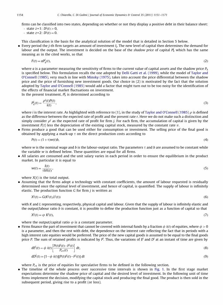
The possible areas of intervention for the policy maker to reduce the volatility of the system are identifiable in thelimitations to the creation of liquid assets and in the regulation of bankruptcy. These two areas are represented,respectively, by the parameters c, which quantifies the capacity of the system to create endogenous money, and c, which isthe maximum debt ratio allowed to avoid failure.

As shown by Fig. 12, the degree of financial innovation and the consequent capacity of the system to create endogenouscredit plays a key role in generating the booms. The availability of easily tradable financial instruments pumps liquidityinto the system augmenting the level of wealth W(t). Credit becomes cheaper and the accumulation of capital occurs at afaster rate. A bigger stock of liquid assets in the market makes possible the accumulation of a larger stock of capital in thelong run. The downside of this is the much larger volatility and the associated long periods of contraction. From thisperspective a regulatory framework for securitization and in general for the creation of financial derivatives may reduce cand be effective in reducing the volatility. Interestingly, for high values of c (above 0.6), the system may become unstableand subjected to waves of failures that involve almost all the active firms.

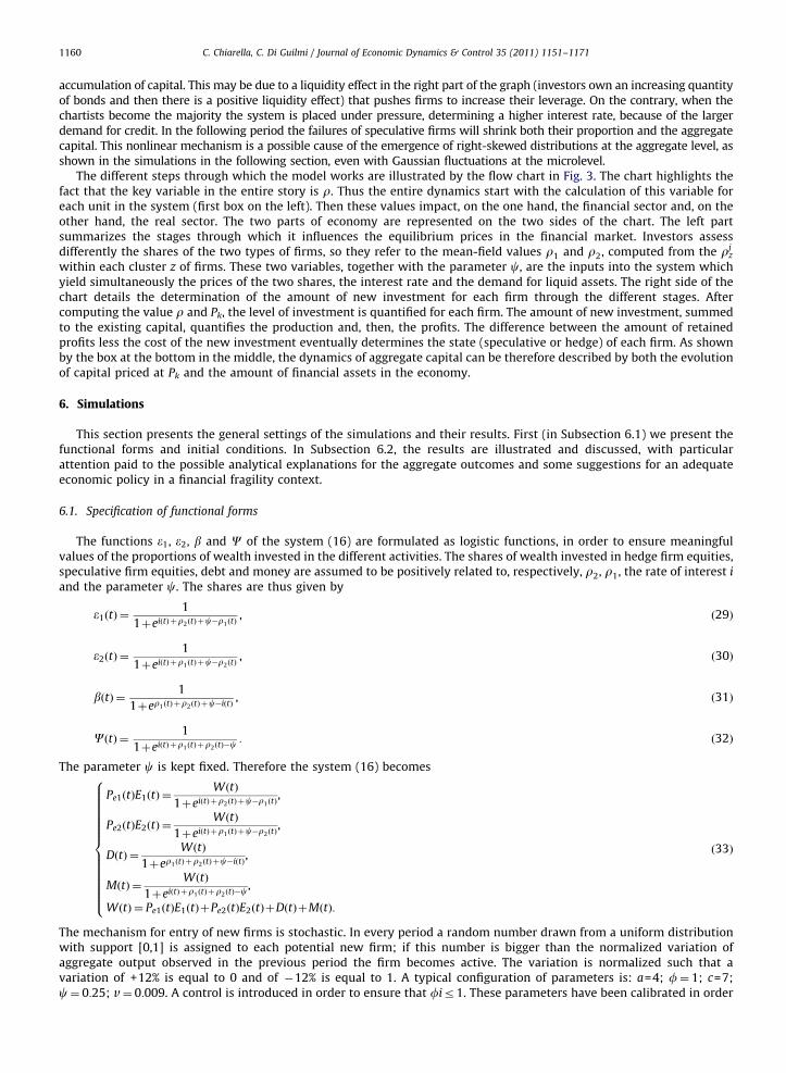
A larger value of the parameter c corresponds to an easing in the position of heavily indebted firms15 or to a temporarysupport to those in a critical condition. The model demonstrates that larger debt ratios can lengthen the positive trend but,as a consequence, the period of distress is longer, increasing the uncertainty in the system (Fig. 13). These results areconsistent with the findings of Suarez and Sussman (2007) that a softening in bankruptcy laws ensures a faster growth atthe expense of long term stability. The degree of uncertainty in the present model can be quantified by the parameter a,which measures the reactions of firms to market expectations, and by the possible changes in investor strategies, capturedby the distribution of nc. As a grows the cycles become more regular, longer and of larger amplitude. Beyond a certain

15 Chapter 11 in the USA and other similar legislations in other countries may be regarded as an example.

Fig. 12. Average aggregate capital, variance of fluctuations, interest rate and final wealth for different values of c. Based on the Monte Carlo simulation of

the agent based model.

Fig. 13. Average aggregate capital, variance of fluctuations, interest rate and final wealth for different values of c. Based on the Monte Carlo simulation of



threshold (a410) the positive long run trend virtually disappears and only long fluctuations are observable. A reduction inthe support for the distribution of nc or a less dispersed distribution (truncated normal rather than a uniform distribution)reduces the average interest rate, allowing a more sustained growth with a slower accumulation of debt.

As regards the choice of firms between equity and debt as source of financing, Fig. 14 shows that as the proportion ofinvestment financed with equity (measured by f) increases, the system becomes more stable. The accumulation of capitalimproves despite the fact that, for low shares of debt financing, private wealth shrinks.

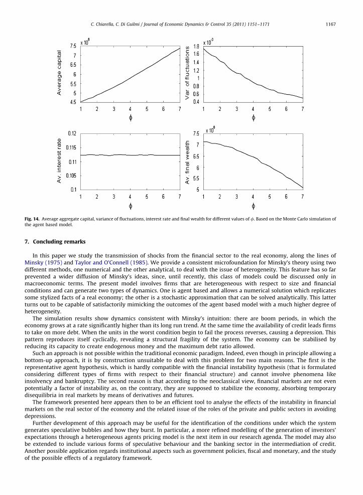
Fig. 14. Average aggregate capital, variance of fluctuations, interest rate and final wealth for different values of f. Based on the Monte Carlo simulation of



7. Concluding remarks

In this paper we study the transmission of shocks from the financial sector to the real economy, along the lines ofMinsky (1975) and Taylor and O’Connell (1985). We provide a consistent microfoundation for Minsky’s theory using twodifferent methods, one numerical and the other analytical, to deal with the issue of heterogeneity. This feature has so farprevented a wider diffusion of Minsky’s ideas, since, until recently, this class of models could be discussed only inmacroeconomic terms. The present model involves firms that are heterogeneous with respect to size and financialconditions and can generate two types of dynamics. One is agent based and allows a numerical solution which replicatessome stylized facts of a real economy; the other is a stochastic approximation that can be solved analytically. This latterturns out to be capable of satisfactorily mimicking the outcomes of the agent based model with a much higher degree ofheterogeneity.

The simulation results show dynamics consistent with Minsky’s intuition: there are boom periods, in which theeconomy grows at a rate significantly higher than its long run trend. At the same time the availability of credit leads firmsto take on more debt. When the units in the worst condition begin to fail the process reverses, causing a depression. Thispattern reproduces itself cyclically, revealing a structural fragility of the system. The economy can be stabilised byreducing its capacity to create endogenous money and the maximum debt ratio allowed.

Such an approach is not possible within the traditional economic paradigm. Indeed, even though in principle allowing abottom-up approach, it is by construction unsuitable to deal with this problem for two main reasons. The first is therepresentative agent hypothesis, which is hardly compatible with the financial instability hypothesis (that is formulatedconsidering different types of firms with respect to their financial structure) and cannot involve phenomena likeinsolvency and bankruptcy. The second reason is that according to the neoclassical view, financial markets are not evenpotentially a factor of instability as, on the contrary, they are supposed to stabilize the economy, absorbing temporarydisequilibria in real markets by means of derivatives and futures.

The framework presented here appears then to be an efficient tool to analyse the effects of the instability in financialmarkets on the real sector of the economy and the related issue of the roles of the private and public sectors in avoidingdepressions.

Further development of this approach may be useful for the identification of the conditions under which the systemgenerates speculative bubbles and how they burst. In particular, a more refined modelling of the generation of investors’expectations through a heterogeneous agents pricing model is the next item in our research agenda. The model may alsobe extended to include various forms of speculative behaviour and the banking sector in the intermediation of credit.Another possible application regards institutional aspects such as government policies, fiscal and monetary, and the studyof the possible effects of a regulatory framework.


Appendix A

This appendix summarises material from Di Guilmi (2008) and Di Guilmi et al. (2010) regarding the asymptoticsolution of the master equation. We can reformulate the master equation (21) using the alternative notation

dPrðNk,tÞ

dt¼ dðNkþ1ÞPrðNkþ1,tÞþbðNk�1ÞPrðNk�1,tÞ�½bðNkÞþdðNkÞ�PrðNk,tÞ: ðA:1Þ

The transition rates l and m are replaced by b and d which denote the birth and death processes while Pr(Nk,t) representsthe probability of having a number k of firm in state 1 at time t. In order to express the transition rates d(Nk) and b(Nk) in ahomogeneous way, we can make use of the lead and lag operators, here indicated as, respectively, L and L�1. Thus we canwrite the transition rates as

L½dðNkÞPðNk,tÞ� ¼ dðNkþ1ÞPðNkþ1,tÞ, ðA:2Þ

L�1½bðNkÞPðNk,tÞ� ¼ dðNk�1ÞPðNk�1,tÞ: ðA:3Þ

Using these operators, the master equation (A.1) can be expressed as

dPrðNk,tÞ

dt¼ ðL�1Þ½dðNkÞPrðNk,tÞ�þðL�1�1Þ½bðNkÞPrðNk,tÞ�: ðA:4Þ

The operators L and L�1 allow us to treat the transition rates in a generic way, regardless of whether they are births ordeaths. Denoting either of them by a(Nk) we write

ðL�1ÞaðNkÞ ¼ aðNkþ1Þ�aðNkÞ ¼X1k ¼ 0

1

k!

@

@Nk

� �k

aðNkÞ�X1k ¼ 0

1

k!

@

@Nk

� �k

aðNk�1Þ, ðA:5Þ

ðL�1�1ÞaðNkÞ ¼ aðNk�1Þ�aðNkÞ ¼�ðaðNkÞ�aðNk�1ÞÞ ¼�X1k ¼ 0

1

k!

@

@Nk

� �k

aðNk�1ÞþX1k ¼ 0

1

k!

@

@Nkþ1

� �k

aðNk�2Þ: ðA:6Þ

Splitting the state variable Nk into its trend and fluctuations component, according to Eq. (22) for Nz, the master equation(A.1) is modified and expressed as a function of the fluctuation component s using the fact that

_PrðNkÞ ¼@Q

@tþ@s

@t

@Q

@s¼ _Q ðsÞ: ðA:7Þ

According to (22), also the transition rates lðN�NkÞ and mNk must be reformulated as functions of s, so that

bðsÞ ¼ l½N�Nm�ffiffiffiffiNp

s�, ðA:8Þ

dðsÞ ¼ m½NmþffiffiffiffiNp

s�: ðA:9Þ

Applying Eqs. (A.5) and (A.6) on the generic transition rates a(s) we get

ðL�1ÞaðsÞ ¼N�1=2 @

@s

� �aðsÞþ

1

2N�1 @

@s

� �2

aðsÞþ � � � , ðA:10Þ

ðL�1�1ÞaðsÞ ¼ �N�1=2 @

@s

� �aðsÞþ

1

2N�1 @

@s

� �2

aðsÞþ � � � ðA:11Þ

with lead and lag operator, respectively, given by

ðL�1Þ ¼N�1=2 @

@s

� �þ

1

2N�1 @

@s

� �2

þ � � � ðA:12Þ

and

ðL�1�1Þ ¼�N�1=2 @

@s

� �þ

1

2N�1 @

@s

� �2

þ � � � : ðA:13Þ

From (22) it also follows that at a constant level of the state variable Nk

@s

@t¼�N1=2 dm

dt, ðA:14Þ

so that Eq. (A.7) can be rewritten as

_Q ðs,tÞ ¼@Q

@t�N1=2 @Q

@s

dm

dt: ðA:15Þ

The master equation can also be formulated using the lead and lag operators in the form

_Q ðs,tÞ ¼ ðL�1Þ½dðsÞQ ðs,tÞ�þðL�1�1Þ½dðsÞQ ðs,tÞ�: ðA:16Þ


Rescaling the time variable according to

t¼ t

N: ðA:17Þ

The master equation (A.15) becomes

_Q ðs,tÞ ¼N�1 @Q

@t �N�1=2 dm

dt@Q

@s: ðA:18Þ

Substituting the (A.10) and (A.11) into the (A.16) and considering that both the (A.16) and (A.18) are master equationswe can write

N�1 @Q

@t �N�1=2 dm

dt@Q

@s¼ ðL�1Þ½mðmþN�1=2sÞQ ðs,tÞ�þðL�1�1Þ½lð1�m�N�1=2sÞQ ðs,tÞ�: ðA:19Þ

Now we expand the new master equation (A.19) in inverse powers of s up to the second order obtaining

N�1 @Q

@t �N�1=2 dm

dt@Q

@s

¼N�1=2 @

@s

� �½dðsÞQ ðs,tÞ�þN�1 1

2

@

@s

� �2

½dðsÞQ ðs,tÞ��N�1=2 @

@s

� �½bðsÞQ ðs,tÞ�þN�1 1

2

@

@s

� �2

½bðsÞQ ðs,tÞ�þ � � �

¼N�1=2 @

@s

� �½ðdðsÞ�bðsÞÞQ ðs,tÞ�þN�1 1

2

@

@s

� �2

½ðbðsÞþdðsÞÞQ ðs,tÞ�þ � � � : ðA:20Þ

Considering that

dðsÞ�bðsÞ ¼ ðlþmÞðNmþffiffiffiffiNp

sÞ�lN¼ ðlþmÞNk�lN,

dðsÞþbðsÞ ¼ ðl�mÞðNmþffiffiffiffiNp

sÞþlN¼ ðl�mÞNkþlN,

it is possible to rewrite Eq. (A.20) as

N�1 @Q

@t�N�1=2 dm

dt@Q

@s¼ ðlþmÞQ ðs,tÞþN�1=2ðdðsÞ�bðsÞÞ

@

@s

� �Q ðs,tÞþN�1 1

2ðbðsÞþdðsÞÞ

@

@s

� �Q ðs,tÞ: ðA:21Þ

We note that

bðsÞ�dðsÞ ¼�ðlþmÞmþlN¼ bðmÞ�dðmÞ, ðA:22Þ

bðsÞþdðsÞ ¼ �ðm�lÞm�lN¼ bðmÞþdðmÞ: ðA:23Þ

Substituting (A.22) and (A.23) into the (A.21) and applying the polynomial identity principle for powers of N of order �1,it is possible to derive the Fokker–Plank equation for Q ðs,tÞ, namely

N�1 @Q

@t ¼ ðd0ðmÞ�b0ðmÞÞ

@

@s

� �Q ðs,tÞþ 1

2dðmÞþbðmÞð Þ

@

@s

� �2

Q ðs,tÞ: ðA:24Þ

This partial differential equation describes the stochastic process in a continuous form indicating explicitly its drift andfluctuations components.

The theoretical probability Z of being in state 1 can be reformulated as the observed frequency Nk=N of firms occupyingstate 1. Accordingly, the transition rates have to be modified and rewritten as

bn ¼ rðNkþ1jNÞ ¼ zNk

N

N�Nk

N,

dn ¼ lðNk�1jNÞ ¼ iNk

N

Nk�1

N:

8>><>>: ðA:25Þ

In each unit of time we can observe an increment or decrement of one unit in Nk. These positive or negative variations areindicated, respectively, by r (a step to the right toward k+1) and by l (a step to the left toward k�1). Introducing the factorNk=N the probability transition z becomes a constant of proportionality between the birth rate per individual and thedeviation from the upper bound N�Nk. In the same way the probability transition i can be interpreted as a constant ofproportionality between the death rate per individual and the deviation from the lower bound or Nk�1. Given that, it ispossible to set the two functions:

lðNkÞ ¼ lNk

N,

mðNkÞ ¼ mNk

N: ðA:26Þ


Expressing the lead and lag operators L(P) and L�1(P) as

LðPrÞ ¼X1u ¼ 1

N�u=2

u!

@

@s

� �u

Q ðs,tÞ, ðA:27Þ

L�1ðPrÞ ¼X1u ¼ 1

ð�ÞuN�u=2

u!

@

@s

� �u

Q ðs,tÞ, ðA:28Þ

after few simple algebraic steps it is possible to write the master equation (A.1) as

dPr

dt¼N�2fm½NkðNkþ1ÞLðPÞþ2nP��l½ðNk�1ÞðN�Nkþ1ÞL�1ðPÞþðN�2nþ1ÞP�g, ðA:29Þ

and then, substituting the formulation of the above indicated operators (A.27) and (A.28) into Eq. (A.29), we obtain

dPr

dt¼N�2

X1u ¼ 1

½DðNkÞþð�ÞuBðNkÞ�

N�u=2

u!

@

@s

� �u

Q ðs,tÞ( )

þN�2f½2gNk�lðN�2nþ1Þ�Q ðs,tÞg, ðA:30Þ

where

BðNkÞ ¼ BðmÞ ¼ l½N2mð1�mÞþN3=2sð1�2mÞþNð2m�s2�1Þþ2N1=2s�1�,

DðNkÞ ¼DðmÞ ¼ m½N2m2þN3=22msþNðmþs2ÞþN1=2s�:

(ðA:31Þ

In order to derive an explicit formulation for N1/u for u¼ 1,2, we expand Eq. (A.30) to the second order, so that

u¼ 1 : N�1=2½DðmÞ�BðmÞ� ¼N3=2½�lmð1�mÞþmm2�þN½2msðlþmÞ�l/sS/sS�

þN1=2½s2ðlþmÞþðm�2lÞmþ1l��2lsþN�1=2ðms�lÞ,

u¼ 2 :N�1

2½DðmÞþBðmÞ� ¼N½lmð1�mÞþmm2�þN1=2½2msðlþmÞ�ls�

þ½s2ðm�lÞþmðmþ2lÞ�l�þN�1=22lsþN�1ðmsþlÞ:

8>>>>>><>>>>>>:

ðA:32Þ

The results can be substituted into Eq. (A.30), yielding the approximate master equation

dPr

dt¼ fN�1=2½�lmð1�mÞþmm2�þN�1½2msðlþmÞ�ls�g

@

@sQ ðs,tÞþf�N�3=2½s2ðlþmÞþðm�2lÞmþl��N�22ls

�N�5=2ðms�lÞg@

@sQ ðs,tÞþ 1

2fN�1½lmð1�mÞþmm2�þN�3=2½2msðlþmÞ�ls�g

@

@s

� �2

Q ðs,tÞ

þ1

2fN�2½s2ðm�lÞþmðmþ2lÞ�l�þN�5=2lsþN�3ðmsþlÞg

@

@s

� �2

Q ðs,tÞ

þfN�1½2mðlþmÞ�l�þN�3=2½2sðlþmÞ��N�2lg: ðA:33Þ

Then we have derived two different formulations for the master equation: Eqs. (A.18) and (A.33). We equate the twoexpressions and collect the terms which have the same power for N up to the second order, namely N�1 and N�1/2.We match them and, considering that all other terms are of higher order, so that they vanish more quickly as N-1, wecan write

�N�1=2 dm

dt@Q

@s¼�N�1=2½lmð1�mÞ�mm2�

@

@sQ ðs,tÞ, ðA:34Þ

N�1 @Q

@t ¼N�1½2mðlþmÞ�l� @@sðsQ ðs,tÞÞþ

N�1

2½lmð1�mÞþmm2�

@

@s

� �2

Q ðs,tÞ: ðA:35Þ

Therefore, the asymptotically approximate solution of the master equation turns out to be composed by the followingsystem of coupled equations:

dm

dt ¼ lm�ðlþmÞm2, ðA:36Þ

@Q

@t ¼ ½2ðlþmÞm�l�@

@sðsQ ðs,tÞÞþ ½lmð1�mÞþmm2�

2

@

@s

� �2

Q ðs,tÞ: ðA:37Þ

The first equation represents the dynamics of the drift. Equating it to 0 it is possible to quantify its stationary value

m� ¼l

lþm : ðA:38Þ

The final step is to identify an asymptotic solution for the Fokker–Planck equation (A.37), that is to say the stationaryprobability for Q ðs,tÞ for limt-1Q ðs,tÞ for the spread s. We indicate with yðsÞ this stationary probability and set the


equilibrium condition _Q ¼ 0. Thus Eq. (A.37) can be expressed as

2½l�2ðlþmÞm��½lm�ð1�m�Þþmm�2�

s¼1

yðsÞ@

@s

� �yðsÞ: ðA:39Þ

Integrating (A.39) with respect to s, we obtain

yðsÞ ¼ Cexpl�2ðlþmÞm�

lm�þðm�lÞm�2s2

� �: ðA:40Þ

Using the result in Eq. (A.38), we finally obtain an explicit formulation for the stationary probability yðsÞ

yðsÞ ¼ Cexp �s2

2s2

� �, s2 ¼

lgðlmÞ2

: ðA:41Þ

References

Alfarano, S., Lux, T., Wagner, F., 2008. Time variation of higher moments in a financial market with heterogeneous agents: an analytical approach. Journalof Economic Dynamics and Control 32, 101–136.

Aoki, M., 1996. New Approaches to Macroeconomic Modeling. Cambridge University Press.Aoki, M., 2002. Modeling Aggregate Behaviour and Fluctuations in Economics. Cambridge University Press.Aoki, M., Yoshikawa, H., 2006. Reconstructing Macroeconomics. Cambridge University Press.Axtell, R., Axelrod, R., Epstein, J.M., Cohen, M.D., 1996. Aligning simulation models: a case study and results. Computational & Mathematical Organization

Theory 1, 123–141.Brock, W.A., Hommes, C.H., 1997. A rational route to randomness. Econometrica 65, 1059–1096.Chiarella, C., Dieci, R., He, X.Z., 2009. Heterogeneity, market mechanisms and asset price dynamics. In: Hens, T., Schenk-Hoppe, K.R. (Eds.), Handbook of

Financial Markets: Dynamics and Evolution. North-Holland, Amsterdam, The Netherlands, pp. 277–344.Chiarella, C., He, X.Z., 2003. Dynamics of beliefs and learning under aL-processes—the heterogeneous case. Journal of Economic Dynamics and Control

27, 503–531.Delli Gatti, D., Di Guilmi, C., Gaffeo, E., Gallegati, M., Giulioni, G., Palestrini, A., 2005a. Firms’ size distribution and growth rates as determinants of business

fluctuations. In: Kirman, A., Salzano, M. (Eds.), Economics: Complex Windows. Springer, Milan, pp. 181–186.Delli Gatti, D., Di Guilmi, C., Gaffeo, E., Giulioni, G., Gallegati, M., Palestrini, A., 2005b. A new approach to business fluctuations: heterogeneous interacting

agents, scaling laws and financial fragility. Journal of Economic Behavior and Organization 56.Delli Gatti, D., Gallegati, M., Minsky, H.P., 1999. Financial institutions, economic policy, and the dynamic behavior of the economy. Macroeconomics

9903009, EconWPA.Di Guilmi, C., 2008. The Generation of Business Fluctuations: Financial Fragility and Mean-Field Interaction. Peter Lang Publishing Group, Frankfurt/M.Di Guilmi, C., Gaffeo, E., Gallegati, M., Palestrini, A., 2005. International evidence on business cycle magnitude dependence: an analysis of 16

industrialized countries, 1881–2000. International Journal of Applied Econometrics and Quantitative Studies 2, 5–16.Di Guilmi, C., Gallegati, M., Landini, S., 2010. Financial fragility, mean-field interaction and macroeconomic dynamics: a stochastic model. In: Salvadori, N.

(Ed.), Institutional and Social Dynamics of Growth and Distribution. Edward Elgar, UK, pp. 323–351.Fontana, G., 2003. Post Keynesian approaches to endogenous money: a time framework explanation. Review of Political Economy 15, 291–314.Gabaix, X., 2009. The granular origins of aggregate fluctuations. NBER Working Papers 15286, National Bureau of Economic Research, Inc.Gaffeo, E., Gallegati, M., Palestrini, A., 2003. On the size distribution of firms. additional evidence from the G7 countries. Physica A: Statistical Mechanics

and Its Applications 324, 117–123.Gallegati, M., Palestrini, A., 2010. The complex behavior of firms’ size dynamics. Journal of Economic Behavior and Organization 75, 69–76.Jarsulic, M., 1989. Endogenous credit and endogenous business cycles. Journal of Post Keynesian Economics 12, 35–48.Jermann, U.J., Quadrini, V., 2009. Macroeconomic effects of financial shocks, SSRN eLibrary.Keen, S., 1995. Finance and economic breakdown: modelling Minsky financial instability hypothesis. Journal of Post Keynesian Economics 17, 607–635.Kindleberger, C., 2005. Manias Panics and Crashes: A History of Financial Crises, fifth ed. Wiley.Kubo, R., Toda, M., Hashitume, N., 1978. Statistical Physics II. Non Equilibrium Statistical Mechanics. Springer-Verlag, Berlin.Landini, S., Uberti, M., 2008. A statistical mechanic view of macro-dynamics in economics. Computational Economics 32, 121–146.Lima, G.T., Meirelles, A.J.A., 2007. Macrodynamics of debt regimes, financial instability and growth. Cambridge Journal of Economics 31, 563–580.Lux, T., 1995. Herd behaviour, bubbles and crashes. Economic Journal 105, 881–896.Minsky, H.P., 1963. Can ‘‘it’’ happen again?. In: Carson, D. (Ed.), Banking and Monetary Studies. Richard D Irwin, Homewood. Reprinted in Minsky, H.P.,

1982. Inflation, Recession and Economic Policy. ME Sharpe, New York.Minsky, H.P., 1975. John Maynard Keynes. Columbia University Press, New York.Minsky, H.P., 1977. A theory of systemic fragility. In: Altman, E.I., Sametz, A.W. (Eds.), Financial Crisis: Institutions and Markets in a Fragile Environment.

John Wiley and Sons, New York.Minsky, H.P., 1982. Inflation, Recession and Economic Policy. ME Sharpe, New York.Minsky, H.P., 2008. Securitization. Economics Policy Note Archive 08-2, Levy Economics Institute.Myers, S.C., Majluf, N.S., 1984. Corporate financing and investment decisions when firms have information that investors do not have. Journal of Financial

Economics 13, 187–221.Stanley, M., Amaral, L., Buldyrev, S., Havlin, S., Leschhorn, H., Maass, P., Salinger, M., Stanley, H., 1996. Scaling behaviour in the growth of companies.

Nature 379, 804–806.Suarez, J., Sussman, O., 2007. Financial distress, bankruptcy law and the business cycle. Annals of Finance 3, 5–35.Taylor, L., O’Connell, S.A., 1985. A Minsky crisis. The Quarterly Journal of Economics 100, 871–885.Tobin, J., 1969. A general equilibrium approach to monetary theory. Journal of Money, Credit and Banking 1, 15–29.Wray, L.R., Tymoigne, E., 2008. Macroeconomics Meets Hyman P. Minsky: the financial theory of investment. Economics Working Paper Archive 543.

Levy Economics Institute.Zeeman, E.C., 1974. On the unstable behaviour of stock exchanges. Journal of Mathematical Economics 1, 39–49.

Documents

The financial instability hypothesis: A stochastic microfoundation framework