Embed Size (px)
Citation preview

The Financial Bubble Experiment:Advanced Diagnostics and Forecasts of Bubble Terminations
Volume III
R. Woodard, D. Sornette, J. Berninger
(The Financial Crisis Observatory)∗
Department of Management, Technology and Economics,ETH Zurich, Kreuzplatz 5, CH-8032 Zurich, Switzerland
(Dated: 2 May 2011)
This is a summary of the third installment of the Financial Bubble Experiment (FBE), wherewe identified 27 asset bubbles in November 2010 and revealed their names on 2 May 2011. Herewe provide the following original documents packaged as one in the following sequence:
1. the initial public summary document of the FBE Vol. III, uploaded on 12 November 2010as v1 at http://arxiv.org/abs/1011.2882 and which includes the digital fingerprint ofthe original Master document of the 27 assets (item 3 in this list);
2. the names, forecast quantiles and final analysis of the 27 bubbles released on 2 May2011;
3. the original Master document identifying the 27 assets, created on 12 November 2010 andwhose checksum (digital fingerprint) appears in the document of item 1).
For the purpose of verifying the checksums of the original Master document (item 3 in the abovelist), it and the rest of the contents of this summary document can be found individually onlineat http://www.er.ethz.ch/fco/index.
The checksums of the document in item 3 are:
Document name
SHA256SUM 4994beab18293be021d751d513b6fec0776fde9cf74c0098f7da8657487d950d
SHA512SUM ee20582b696a2ce880870b513e7b9e7ebb67bfbe62e2cad50dd18276a5158765af6fdf88d9fef6e047526c40478a865c722cab041386aa8efdd95da24dd9239d
TABLE I. Checksums of Financial Bubble Experiment Vol. III forecast document.
The tables on the following page list the names and forecast quantiles of the 27 assets andare reproduced from item 2 above.

2 H1 Assets (identified bubble)
Category Asset Ticker H1 C
Index MERVAL Buenos Aires ^MERV (Y) 1 *
Equity AUTOZONE AZO (Y) 1
TABLE II. 2 H1 assets of the Financial Bubble Experiment as of 12 November 2010. All listed assetsare candidates for H1 (identified bubble phase). In the Ticker column, (B) stands for Bloomberg and(Y) for Yahoo Finance. Columns ‘H1’ and ‘H2’ show a somewhat subjective score of -1 (worst), 0 or1 (best), reflecting the quality of the forecasts. This scoring is discussed further in Section III of themain analysis document available at http://www.er.ethz.ch/fco/index. Column ‘C’ has an asterisk ifan asset had a major correction within 3 days of t2 =2010-11-10 (the last data observation used in ouranalysis). This correlated dynamics also is discussed in Section III of the same analysis document.
25 H1 and H2 Assets (identified bubble)
Category Asset Ticker tc 20% - 80% tc 5% - 95% H1 H2 C
Index
BSE SENSEX, Bombay ^BSESN (Y) 2010-11-03 - 2010-12-01 2010-10-27 - 2010-12-10 0 1 *
Dow Jones-AIG Comm. ^DJC (Y) 2010-11-16 - 2010-12-04 2010-11-09 - 2010-12-10 1 1 *
FTSE 100 ^FTSE (Y) 2010-11-27 - 2010-12-26 2010-11-07 - 2011-01-03 1 1 *
Hang Seng Index ^HSI (Y) 2010-11-09 - 2010-12-09 2010-11-07 - 2010-12-16 1 1 *
Interactive Week Internet ^IIX (Y) 2010-11-12 - 2010-12-10 2010-11-04 - 2010-12-23 1 1 *
NASDAQ Computer ^IXK (Y) 2010-11-13 - 2010-12-06 2010-11-07 - 2010-12-09 1 1 *
Jakarta Composite ^JKSE (Y) 2010-11-06 - 2010-12-09 2010-10-23 - 2010-12-25 0 0
KOSPI Composite Index ^KS11 (Y) 2010-11-15 - 2010-12-26 2010-10-30 - 2011-01-07 1 0 *
NASDAQ-100 (DRM) ^NDX (Y) 2010-11-05 - 2010-11-29 2010-11-03 - 2010-12-22 1 1 *
Reuters/Jefferies CRB CRY INDEX (B) 2010-11-11 - 2010-11-22 2010-11-07 - 2010-11-26 1 1 *
TSEC weighted index ^TWII (Y) 2010-12-01 - 2011-01-03 2010-11-13 - 2011-01-08 1 -1 *
Major Market Index ^XMI (Y) 2010-11-10 - 2010-11-25 2010-10-30 - 2010-12-04 1 1 *
Equity
Ishares Singapore Index EWS (Y) 2010-11-14 - 2010-12-12 2010-11-06 - 2010-12-25 1 1 *
Freeport McMoRan FCX (Y) 2010-11-15 - 2010-12-17 2010-11-09 - 2010-12-27 1 1 *
F5 NETWORKS FFIV (Y) 2010-12-27 - 2011-03-09 2010-12-02 - 2011-04-08 1 1
INTUIT INTU (Y) 2010-11-28 - 2011-01-15 2010-11-07 - 2011-02-11 0 0 *
STARBUCKS SBUX (Y) 2010-11-08 - 2010-11-18 2010-11-06 - 2010-11-25 1 -1
UNITED RENTALS INC URI (Y) 2010-11-09 - 2010-12-13 2010-11-02 - 2011-01-08 1 -1
Commodity
Copper future (USD) HG1 COMB Comdty (B) 2010-11-09 - 2011-01-07 2010-10-31 - 2011-01-15 1 1 *
Corn future (CHF) C 1 COMB Comdty (B) 2010-11-18 - 2010-12-19 2010-11-08 - 2010-12-28 1 1 *
Cotton future (USD) CT1 COMB Comdty (B) 2010-11-12 - 2010-11-13 2010-11-08 - 2010-11-15 1 1 *
Palladium future (USD) PA1 COMB Comdty (B) 2010-11-12 - 2010-11-19 2010-11-10 - 2010-11-27 1 0 *
Silver future (CHF) SI1 COMB Comdty (B) 2010-11-13 - 2010-11-18 2010-11-08 - 2010-11-29 1 0 *
Sugar future (CHF) SB1 COMB Comdty (B) 2010-11-20 - 2010-12-09 2010-11-10 - 2010-12-17 1 1 *
Forex AUDUSD (B) 2010-11-12 - 2010-12-25 2010-10-30 - 2011-01-12 1 1 *
TABLE III. 25 H2 assets of the Financial Bubble Experiment as of 12 November 2010. All listed assetsare candidates for H1 (identified bubble phase) and H2 (identification of end of bubble phase). Quantilewindows of most likely dates of the end of the bubble phases are shown. Abbreviations (B), (Y), H1, H2and C are described in caption of Table II.
Item 1:Initial public summary document of
the FBE Vol. III,as uploaded on 12 November 2010 as v1
athttp://arxiv.org/abs/1011.2882

The Financial Bubble Experiment:Advanced Diagnostics and Forecasts of Bubble Terminations
Volume III–Master Document
R. Woodard, D. Sornette, M. Fedorovsky
(The Financial Crisis Observatory)∗
Department of Management, Technology and Economics,ETH Zurich, Kreuzplatz 5, CH-8032 Zurich, Switzerland
(Dated: 11 November 2010)
This is the third installment of the Financial Bubble Experiment. Here we provide the digitalfingerprint of an electronic document [1] in which we identify 27 bubbles in 27 different global assets;for 25 of these assets, we present windows of dates of the most likely ending time of each bubble.We will provide that document of the original analysis on 2 May 2011.
I. INTRODUCTION
The Financial Bubble Experiment (FBE) aims at testing the following two hypotheses:
• Hypothesis H1: Financial (and other) bubbles can be diagnosed in real-time before they end.
• Hypothesis H2: The termination of financial (and other) bubbles can be bracketed using probabilistic forecasts,with a reliability better than chance.
In a medical context, H1 corresponds to the diagnostic of cancer and H2 to the forecast of remaining life expectancy.The motivation of the Financial Bubble Experiment finds its roots in the failure of standard approaches. Indeed,
neither the academic nor professional literature provides a clear consensus for an operational definition of financialbubbles or techniques for their diagnosis in real time. Instead, the literature reflects a permeating culture that simplyassumes that any forecast of a bubble’s demise is inherently impossible.
Because back-testing is subjected to a host of possible biases, we propose the FBE as a real-time advanced forecastmethodology that is constructed to be free, as much as possible, of all possible biases plaguing previous tests ofbubbles. In particular, active researchers are constantly tweaking their procedures, so that predicted ‘events’ becomemoving targets. Only advance forecasts can be free of data-snooping and other statistical biases of ex-post tests. TheFBE aims at rigorously testing bubble predictability using methods developed in our group and by other scholarsover the last decade. The main concepts and techniques used for the FBE have been documented in numerous papers[2–6] and the book [7].
In the FBE, we propose a new method of delivering our forecasts where the results are revealed only after thepredicted event has passed but where the original date when we produced these same results can be publicly, digitallyauthenticated. Since our science and techniques involve forecasting, the best test of a forecast is to publicize it andwait to see how accurate it is, whether the wait involves days, weeks or months (we rarely make forecasts for longertime scales). We will do this and at the same time we want to delay the unveiling of our results until after theforecasted event has passed to avoid potential issues of liability, ethics and speculation. Also, we think that a full setof results showing multiple forecasts all at once is more revealing of the quality of our current methods than wouldbe a trickle of one such forecast every month or so. We also want to address the obvious criticism of cherry pickingsuccessful forecasts, as explained below. In order to be convincing, our experiment has to report all cases, be theysuccesses or failures.
The digital fingerprint of our first set of bubble forecasts was released on 2 November 2009 (with a hash update on6 November 2009). We added a new bubble forecast on 23 December 2009. The original forecasts and post-analysiswere presented publicly on 3 May 2010 and uploaded to the arxiv server on 14 May 2010. All versions are availableat [8].
This third set of forecasts presents the methodology described in [8] and the digital fingerprint of a single documentthat identifies and analyses 27 current asset bubbles (H1). For 25 of those 27 bubbles, the document also provideswindows of dates of the most likely ending time of each bubble. We will provide that original document of the analysison 2 May 2011.
2
II. DESCRIPTION OF THE METHODOLOGY OF THE FINANCIAL BUBBLE EXPERIMENT
Our method for this experiment is the following:
• We choose a series of dates with a fixed periodicity on which we will reveal our forecasts and make these datespublic by immediately posting them on our University web site and on the first version of our main publication,which we describe below. Specifically, our first publication of the forecasts was issued on 3 May 2010, withsuccessive deliveries every 6 months. The forecasts of the current document will be presented on 2 May 2011.However, we keep open the option of changing the periodicity of the future deliveries as the experiment unfoldsand we learn from it and from feedback of the scientific community.
• We then continue our current research involving analysis of thousands of global financial time series.
• When we have a confident forecast, we summarize it in a simple .pdf document.
• We do not make this document public. Instead, we make its digital fingerprint public. We generate two digitalfingerprints for each document, with the publicly available 256 and 512 bit versions of the SHA-2 hash algorithm[9] [10]. This creates two strings of letters and numbers that are unique to this file. Any change at all in thecontents of this file will result in different SHA-2 signatures.
• We create the first version of our main document (this one), containing a brief description of our theory andmethods, the SHA-2 hashes of our forecast and the date (2 May 2011) on which we will make the original .pdfdocument public.
• We upload this main ‘meta’ document to http://arxiv.org. This makes public our experiment and the SHA-2hashes of our forecast. In addition, it generates an independent timestamp documenting the date on which wemade (or at least uploaded) our forecast. arxiv.org automatically places the date of when the document wasfirst placed on its server as ‘v1’ (version 1). It is important for the integrity of the experiment that this date isdocumented by a trusted third party.
• We continue our research until we find our next confident forecast. We again put the forecast results in a .pdfdocument and generate the SHA-2 hashes. We now update our master document with the date and digitalfingerprint of this new forecast and upload this latest version of the master document to arxiv.org. The serverwill call this ‘v2’ (version 2) of the same document while keeping ‘v1’ publicly available as a way to ensureintegrity of the experiment (i.e., to ensure that we do not modify the SHA-2 hashes in the original document).Again, ‘v2’ has a timestamp created by arxiv.org.
• Notice that each new version contains the previous SHA-2 signatures, so that in the end there will be a list ofdates of publication and associated SHA-2 signatures.
• We continue this protocol until the future date (2 May 2011) at which time we upload our final version of themaster document. For this final version, we include the URL of a web site where the .pdf documents of all ofour past forecasts can be downloaded and independently checked for consistent SHA-2 hashes. For convenience,we will include a summary of all of our forecasts in this final document.
Note that the above method implies two aspects of the same important check to the integrity of our experiment:
1. We will reveal all forecasts, be they successful or not.
2. We will not simply ‘cherry-pick’ the results that we would want the community to see (with a few token, possibly,bad results). We do not have another simultaneous outlet where we are running a similar experiment, sincearxiv.org is a very visible international platform.
III. BACKGROUND AND THEORY
Our theories of financial bubbles and crashes have been well-researched and documented over the past 15 years inmany papers and books. We refer the reader to the Bibliography. In particular, broad overviews can be found in[2–6]. In short, our theories are based on positive feedback on the growth rate of an asset’s price by price, returnand other financial and economic variables, which lead to faster-than-exponential (power law) growth. The positivefeedback is partially due to imitation and herding among humans, who are actively trading the asset. This signature is

3
quantitatively identified in a time series by a faster-than-exponential power law component, the existence of increasinglow-frequency volatility, these two ingredients occurring either in isolation or simultaneously with varying relativeamplitudes. A convenient representation has been found to be the existence of a power law growth decorated byoscillations in the logarithm of time. The simplest mathematical embodiment is obtained as the first order expansionof the log-periodic power law (LPPL) model and is shown in Eq. (1):
lnP = A+B|t− tc|α + C|t− tc|α cos[ω ln |t− tc|+ φ] (1)
where P is the price of the asset and t is time. There are 7 parameters in this nonlinear equation, whose relativeimportance and estimation are described in our previous papers [2–6]. Our past work has led to the hypothesis thatthe LPPL signals can be useful precursors to an ending (change of regime) of the bubble, either in a crash or aless-dramatic leveling off of the growth.
IV. METHODS
A. Bubble identification
As are our theories, our methods are documented elsewhere so we only briefly mention the general technique sothat the forecasts that we make public can be better understood. In short, we scan thousands of financial time serieseach week and identify regions in the series that are well-fit by Eq. (1). We divide each time series into sub-seriesdefined by start and end times, t1 and t2 and then fit each sub-series (t1, t2). We choose max(t2) as the date of themost recent available observation. Many sub-series are created according to the following parameters: dt1 = dt2 = 7days, min(t2 − t1) = 91 days and max(t2 − t1) = 1092 days.
After filtering all fits with an appropriate range of parameters, we select those assets that have the strongest LPPLsignatures. To improve statistics, we can calculate the residues between the model and the observations and use theresidues to create 10 synthetic datasets (bootstraps) that have similar statistics as the original time series. We fitEq. (1) to the synthetic data and then extrapolate this entire ensemble of LPPL models to six months beyond our lastobservation. One of the parameters in the LPPL equation is the “crash” time tc, which represents the most probabletime of the end of the bubble and change of regime. We identify the 20%/80% and 5%/95% quantiles of tc of thefits of the ensemble consisting of original fits and bootstrap fits. These two sets of quantiles, the date of the lastobservation and the number of fits in the ensemble are published in our forecasts.
B. Post-analysis
Once the .pdf documents with the full description of the forecasts are made public, the question arises as howto evaluate the quality of the diagnostics and how these results help falsify the two hypotheses? In a nutshell, theproblem boils down to qualifying (and quantifying) what is meant by (i) a successful diagnostic of the existence of abubble and (ii) a successful forecast of the termination of the bubble. In the end, one would like to develop statisticaltests to falsify the two hypotheses stated above, using the track record that the present financial bubble experimenthas the aim to construct. For instance, Chapter 9 of (Sornette, 2003) suggests a number of options, including the“statistical roulette”, Bayesian inference and error diagrams. Our main goal with this FBE is to timestamp ourforecasts as we simultaneously continue our search for adequate measures to qualify the quality of our forecasts.
This quantification is an active, ongoing subset of our research. We are currently developing and testing novelestimations methods that will be progressively implemented in future releases. For our previous forecasts, we quantifiedthe quality of the forecasts with four measures that we will continue to use in the final analysis:
• Drawdown analysis: Drawdown analysis simply identifies the largest drawdown observed between t2 (dateof forecast) and the date of the public ‘unveiling’ of the original forecasts. That is, we identify the largestdrawdown in all available data after t2. A drawdown is simply defined as the largest peak-to-trough drop inprice in a given region.
• Fraction of up days in a running window: We calculate one day close-to-close returns for each asset andmark them as positive (up) or non-positive (zero or down). The ratio of up days relative to the sum of up anddown days in a running window of 30, 60 or 90 days is plotted on top of the price observations.
• Derivative of observations: Another measure of the change of regime is provided by an estimation of the localgrowth rate. We use the Savitzky-Golay smoothing algorithm to calculate the first derivative of the observations,using a third order polynomial fit centered within windows of 120 and 180 days.

4
• Bubble index: A measure we are developing that quantifies the quality of the LPPL fits to the price timeseries.
We are developing other measures that will be used in future analysis.
V. BUBBLE FORECASTS
The checksums of the analysis document [1] that contains the names of the 27 assets are shown in Table I. Thisdocument showing all 27 assets and 25 forecasts, as well as analysis of each identified bubble, will be uploaded tohttp://www.er.ethz.ch/fco/ on 2 May 2011.
Document name
SHA256SUM 4994beab18293be021d751d513b6fec0776fde9cf74c0098f7da8657487d950d
SHA512SUM ee20582b696a2ce880870b513e7b9e7ebb67bfbe62e2cad50dd18276a5158765af6fdf88d9fef6e047526c40478a865c722cab041386aa8efdd95da24dd9239d
TABLE I. Checksums of Financial Bubble Experiment Vol. III forecast document.
[1] R. Woodard, D. Sornette, and M. Fedorovsky (The Financial Crisis Observatory), “The Financial Bubble Experi-ment: advanced diagnostics and forecasts of bubble terminations, Vol. III–assets document,” (2011), to be posted athttp://www.er.ethz.ch/fco/ on 2 May 2011.
[2] Z.-Q. Jiang, W.-X. Zhou, D. Sornette, R. Woodard, K. Bastiaensen, and P. Cauwels, Journal of Economic Behavior &Organization 74, 149 (2010), ISSN 0167-2681, http://www.sciencedirect.com/science/article/B6V8F-4YK2DY8-1/2/3e0bc3155eed4914a7987ddd9ca7789e.
[3] A. Johansen, D. Sornette, and O. Ledoit, J. Risk 1, 5 (1999).[4] A. Johansen and D. Sornette, Brussels Economic Review 49 (2006), (http://arXiv.org/abs/cond-mat/0210509).[5] D. Sornette and A. Johansen, Quant. Financ. 1, 452 (2001).[6] D. Sornette and W.-X. Zhou, Int. J. Forecast. 22, 153 (2006).[7] D. Sornette, Why Stock Markets Crash: Critical Events in Complex Financial Systems (Princeton University Press, Prince-
ton, 2003).[8] D. Sornette, R. Woodard, M. Fedorovsky, S. Reimann, H. Woodard, and W.-X. Zhou (The Financial Crisis Ob-
servatory), “The Financial Bubble Experiment: advanced diagnostics and forecasts of bubble terminations,” (2009),http://arxiv.org/abs/0911.0454.
[9] http://en.wikipedia.org/wiki/SHA_hash_functions.[10] http://eprint.iacr.org/2008/270.pdf.
Item 2:Final analysis of the 27 bubbles,
released on 2 May 2011.

The Financial Bubble Experiment:Advanced Diagnostics and Forecasts of Bubble Terminations
Volume III–Final Analysis
R. Woodard, D. Sornette, J. Berninger
(The Financial Crisis Observatory)∗
Department of Management, Technology and Economics,ETH Zurich, Kreuzplatz 5, CH-8032 Zurich, Switzerland
(Dated: 2 May 2011)
This is the third installment of the Financial Bubble Experiment. Here we provide analysis ofthe 27 bubbles identified in the electronic document [1], whose digital fingerprint was published onarxiv.org on 12 November 2010 [2]. The abstract is purposefully succinct and without summary andconclusions in order to avoid influencing the reader and allow him/her to form his/her conclusions.
CONTENTS
I. Introduction 3
II. Executive summary of the results 3A. H1: Identification of a bubble 4B. H2: Forecast of change of regime 4
III. Explanation of analysis measures 4
IV. Results of Simple Trading Strategies 6
V. Analysis of H1 Assets 8A. H1 Indexes 9
1. MERVAL Buenos Aires 9B. H1 Equities 11
1. AUTOZONE 11
VI. Analysis of H1 & H2 Assets 13A. H1 & H2 Indexes 14
1. BSE SENSEX, Bombay 142. Dow Jones-AIG Commodity Index 163. FTSE 100 184. Hang Seng Index Hong Kong 205. Interactive Week Internet Index 226. NASDAQ Computer 247. Jakarta Composite 268. KOSPI Composite Index, Seoul 289. NASDAQ-100 (DRM) 30
10. Reuters/Jefferies CRB index 3211. TSEC weighted index 3412. Major Market Index 36
B. H1 & H2 Equities 381. Ishares Singapore Index 382. Freeport McMoRan Copper & Gold 403. F5 NETWORKS 424. INTUIT 445. STARBUCKS 466. UNITED RENTALS INC 48
C. H1 & H2 Commodities 50

2
1. Copper future (USD) 502. Corn future (CHF) 523. Cotton future (USD) 544. Palladium future (USD) 565. Silver future (CHF) 586. Sugar future (CHF) 60
D. H1 & H2 Foreign Exchange 621. AUDUSD 62
VII. State of the Market at Time of Analysis (November 2010) 64
References 65
3
I. INTRODUCTION
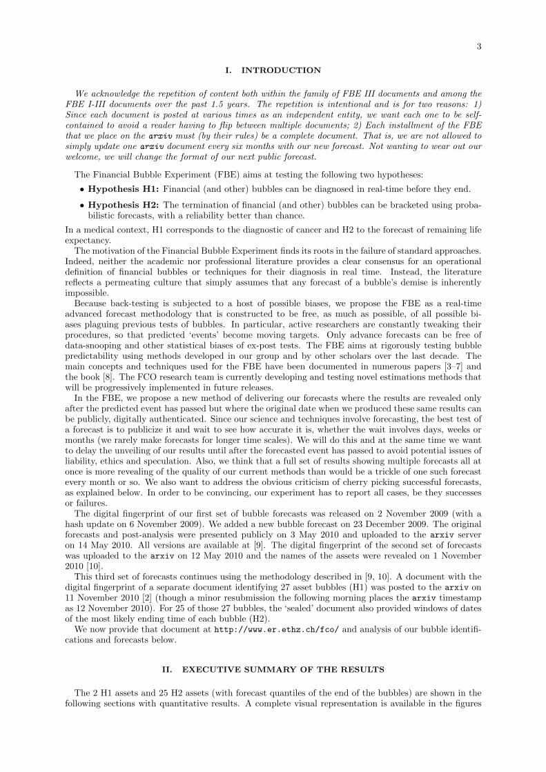
We acknowledge the repetition of content both within the family of FBE III documents and among theFBE I-III documents over the past 1.5 years. The repetition is intentional and is for two reasons: 1)Since each document is posted at various times as an independent entity, we want each one to be self-contained to avoid a reader having to flip between multiple documents; 2) Each installment of the FBEthat we place on the arxiv must (by their rules) be a complete document. That is, we are not allowed tosimply update one arxiv document every six months with our new forecast. Not wanting to wear out ourwelcome, we will change the format of our next public forecast.
The Financial Bubble Experiment (FBE) aims at testing the following two hypotheses:
• Hypothesis H1: Financial (and other) bubbles can be diagnosed in real-time before they end.
• Hypothesis H2: The termination of financial (and other) bubbles can be bracketed using proba-bilistic forecasts, with a reliability better than chance.
In a medical context, H1 corresponds to the diagnostic of cancer and H2 to the forecast of remaining lifeexpectancy.
The motivation of the Financial Bubble Experiment finds its roots in the failure of standard approaches.Indeed, neither the academic nor professional literature provides a clear consensus for an operationaldefinition of financial bubbles or techniques for their diagnosis in real time. Instead, the literaturereflects a permeating culture that simply assumes that any forecast of a bubble’s demise is inherentlyimpossible.
Because back-testing is subjected to a host of possible biases, we propose the FBE as a real-timeadvanced forecast methodology that is constructed to be free, as much as possible, of all possible bi-ases plaguing previous tests of bubbles. In particular, active researchers are constantly tweaking theirprocedures, so that predicted ‘events’ become moving targets. Only advance forecasts can be free ofdata-snooping and other statistical biases of ex-post tests. The FBE aims at rigorously testing bubblepredictability using methods developed in our group and by other scholars over the last decade. Themain concepts and techniques used for the FBE have been documented in numerous papers [3–7] andthe book [8]. The FCO research team is currently developing and testing novel estimations methods thatwill be progressively implemented in future releases.
In the FBE, we propose a new method of delivering our forecasts where the results are revealed onlyafter the predicted event has passed but where the original date when we produced these same results canbe publicly, digitally authenticated. Since our science and techniques involve forecasting, the best test ofa forecast is to publicize it and wait to see how accurate it is, whether the wait involves days, weeks ormonths (we rarely make forecasts for longer time scales). We will do this and at the same time we wantto delay the unveiling of our results until after the forecasted event has passed to avoid potential issues ofliability, ethics and speculation. Also, we think that a full set of results showing multiple forecasts all atonce is more revealing of the quality of our current methods than would be a trickle of one such forecastevery month or so. We also want to address the obvious criticism of cherry picking successful forecasts,as explained below. In order to be convincing, our experiment has to report all cases, be they successesor failures.
The digital fingerprint of our first set of bubble forecasts was released on 2 November 2009 (with ahash update on 6 November 2009). We added a new bubble forecast on 23 December 2009. The originalforecasts and post-analysis were presented publicly on 3 May 2010 and uploaded to the arxiv serveron 14 May 2010. All versions are available at [9]. The digital fingerprint of the second set of forecastswas uploaded to the arxiv on 12 May 2010 and the names of the assets were revealed on 1 November2010 [10].
This third set of forecasts continues using the methodology described in [9, 10]. A document with thedigital fingerprint of a separate document identifying 27 asset bubbles (H1) was posted to the arxiv on11 November 2010 [2] (though a minor resubmission the following morning places the arxiv timestampas 12 November 2010). For 25 of those 27 bubbles, the ‘sealed’ document also provided windows of datesof the most likely ending time of each bubble (H2).
We now provide that document at http://www.er.ethz.ch/fco/ and analysis of our bubble identifi-cations and forecasts below.
II. EXECUTIVE SUMMARY OF THE RESULTS
The 2 H1 assets and 25 H2 assets (with forecast quantiles of the end of the bubbles) are shown in thefollowing sections with quantitative results. A complete visual representation is available in the figures

4
in Sections V-VI.We confirm ‘bubble’ by an ex-post inspection of the price times series: a major downward change
in the growth rate of the price time series within the six months after our analysis indicates that theasset had been in a bubble. Because the definition of what is a “major downward change” is prone topossible subjective and a posteriori tweaking, we offer several metrics described below: (i) drawdowns,(ii) fraction of up days in running windows, and (iii) derivative of the log-price (providing an estimate ofthe trend). In general, our bubble theory says that a bubble ends in a change of regime, that is, whenthe super-exponential growth rate ends. This could range from a simple lessening of the growth rateto a large crash. One of the most frequent types of change of regime that we observed in this currentexperiment occurred when the price time series exhibited a well-defined correction or crash within 6months immediately following the date of when the initial document was posted to the arxiv on 12November 2010 [2].
A. H1: Identification of a bubble
We support H1 by confirming that bubbles existed in 24 of the 27 assets at the time of the lastobservation of our forecasts, t2 = 10 November 2010.
B. H2: Forecast of change of regime
We support H2 by confirming that 17 of the 25 H2 assets showed substantial corrections in the quantilewindows that we forecast.
III. EXPLANATION OF ANALYSIS MEASURES
In the following subsections, we include figures for each asset. The figures share some common features,explained here. Details for each individual asset and measure are discussed below.
Axes and observations: Price (or value of the asset) is shown on the left vertical axis and calendardays are indicated on the bottom horizontal axis. The circles represent closing price observations ontrading days. Note that the price axis shows observations in their natural units on a logarithmic scale.
Large shaded region, vertical and horizontal black lines: The large grey shaded regions thatbegin near the left price axis and end at the solid black vertical line near the right vertical axis representthe domain of the observations used in our analysis. The vertical line itself sits at t2 = 10 November2010: the last observation used in the analysis. The price at t2 is represented by the solid black horizontalline.
Small hatched, shaded regions: Two hatched shaded regions begin in the vicinity of t2. Theyrepresent our forecast “danger” zones, where changes of regimes are most likely to occur. The inner,narrow one with diagonal hatching represents the 20-80% quantile interval and the outer, wider onewith horizontal hatching represents the 5-95% quantile interval. That is, these two numbers imply a 60%(respectively, 90%) probability for the end of the bubble to be located within the diagonally (respectively,horizontally) hatched zone. The hatched shaded regions are presented for all 27 assets, even the two(MERVAL and AZO) for which we did not publish forecasts.
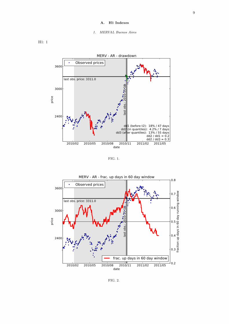
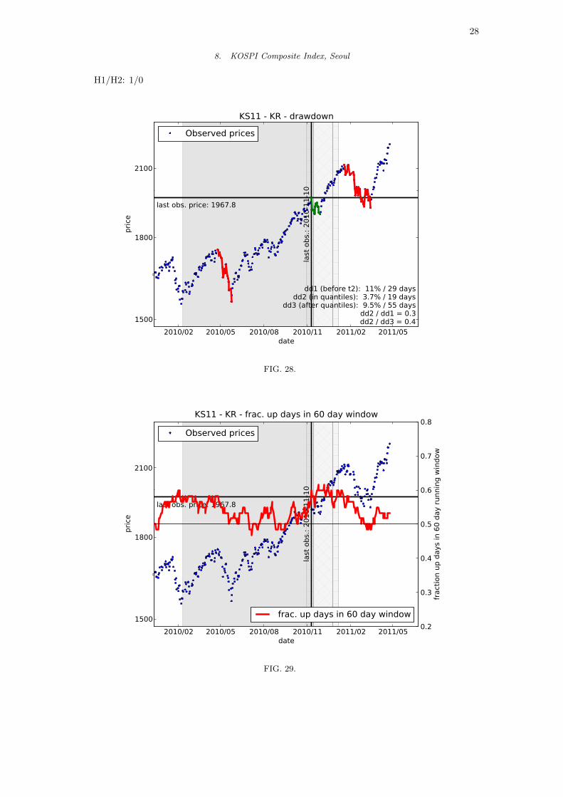
Drawdown analysis: Drawdown analysis figures show a solid red or green line connecting the pathof the largest drawdown observed in three distinct sections:
1. between the beginning of the domain of analysis (left edge of large shaded grey region) and t2 (redline);
2. between the 5% and 95% forecast windows (green line);
3. between the 95% quantile line and 27 April 2011 (red line).
5
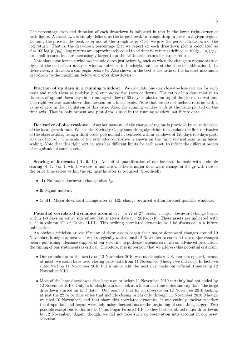
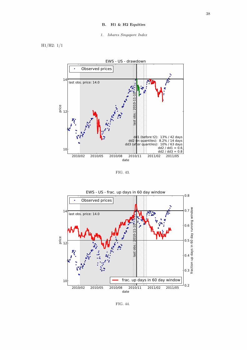
The percentage drop and duration of each drawdown is indicated in text in the lower right corner ofeach figure. A drawdown is simply defined as the largest peak-to-trough drop in price in a given region.Defining the price at the peak as p1 and at the trough as p2 < p1, we give the percent drawdown of thelog return. That is, the drawdown percentage that we report on each drawdown plot is calculated asd = 100 log(p1/p2). Log returns are approximately equal to arithmetic returns (defined as 100(p1−p2)/p1)for small returns but are increasingly larger than the arithmetic return for larger returns.
Note that some forecast windows include dates just before t2, such as when the change in regime startedright at the end of our analysis window (obvious in hindsight but not at the time of publication!). Inthese cases, a drawdown can begin before t2. Also shown in the text is the ratio of the forecast maximumdrawdown to the maximum before and after drawdowns.
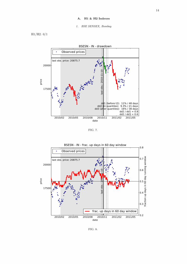
Fraction of up days in a running window: We calculate one day close-to-close returns for eachasset and mark them as positive (up) or non-positive (zero or down). The ratio of up days relative tothe sum of up and down days in a running window of 60 days is plotted on top of the price observations.The right vertical axis shows this fraction on a linear scale. Note that we do not include returns with avalue of zero in the calculation of this ratio. Also, the running window ends at the value plotted on thetime axis. That is, only present and past data is used in the running window, not future data.
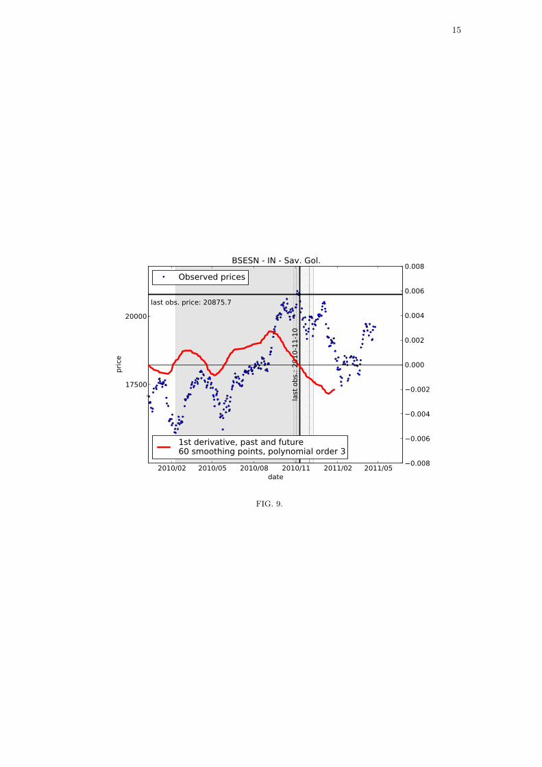
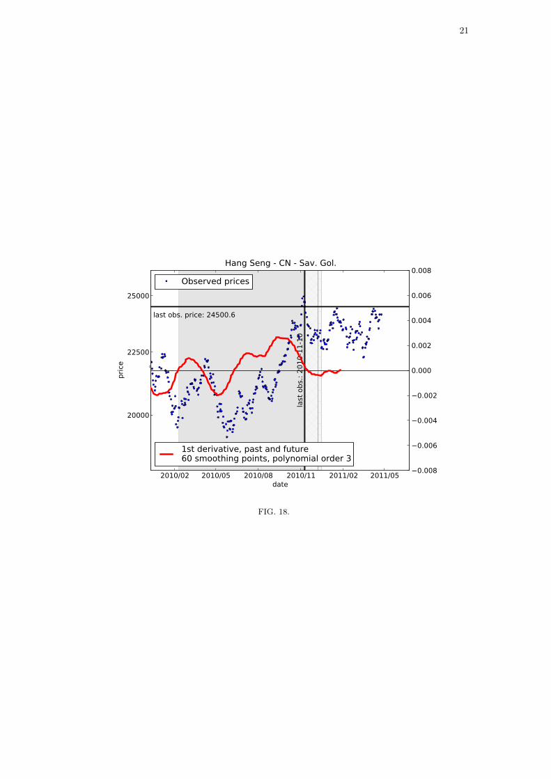
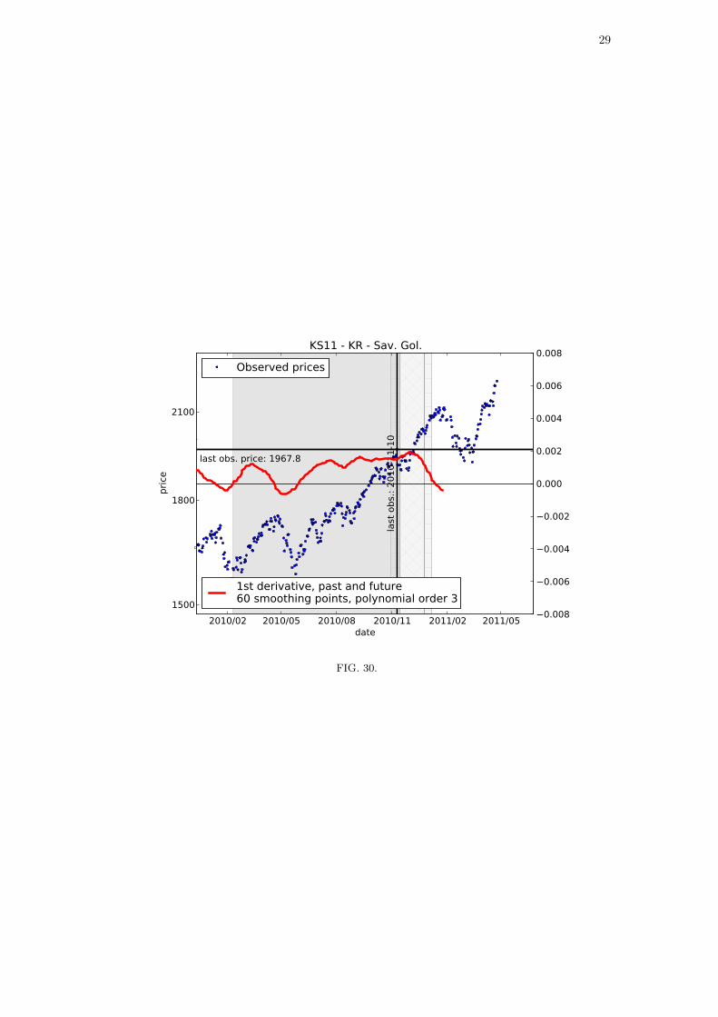
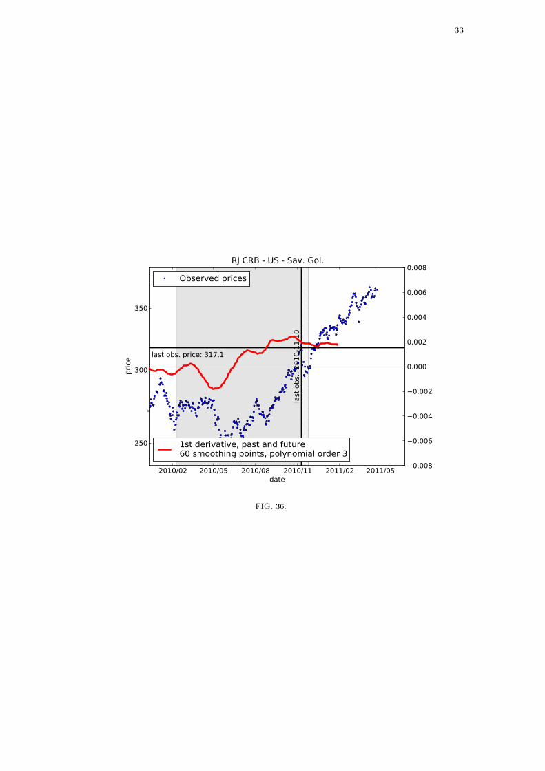
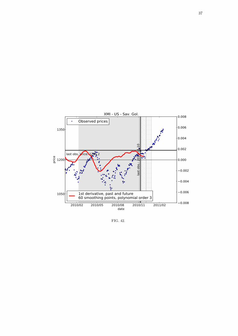
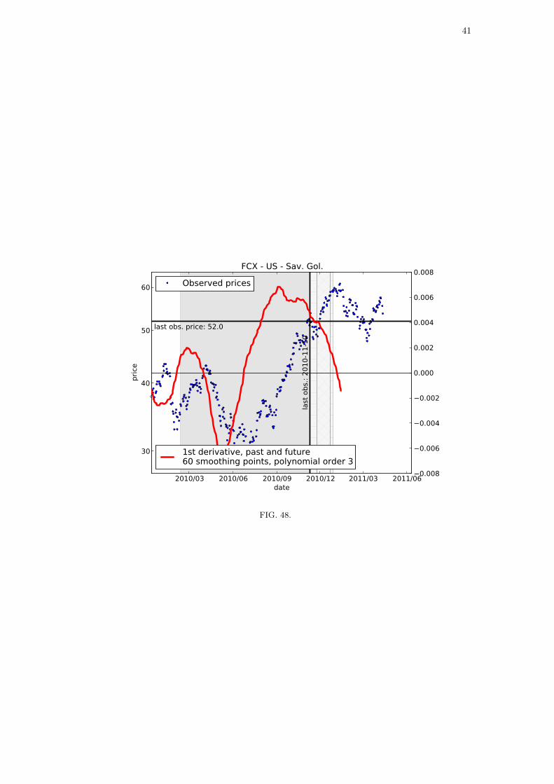
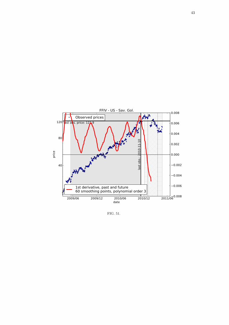
Derivative of observations: Another measure of the change of regime is provided by an estimationof the local growth rate. We use the Savitzky-Golay smoothing algorithm to calculate the first derivativeof the observations, using a third order polynomial fit centered within windows of 120 days (60 days past,60 days future). The scale of the estimated derivative is shown on the right vertical axis using linearscaling. Note that this right vertical axis has different limits for each asset, to reflect the different ordersof magnitude of some assets.
Scoring of forecasts (-1, 0, 1): An initial quantification of our forecasts is made with a simplescoring of -1, 0 or 1, which we use to indicate whether a major downward change in the growth rate ofthe price time series within the six months after t2 occurred. Specifically:
• -1: No major downward change after t2.
• 0: Signal unclear.
• 1: H1: Major downward change after t2; H2: change occurred within forecast quantile windows.
Potential correlated dynamics around t2. In 22 of 27 assets, a major downward change beganwithin 1-3 days on either side of our last analysis date t2 =2010-11-10. These assets are indicated witha ‘*’ in column ‘C’ of Tables II-III. This striking correlated dynamics will be discussed in a futurepublication.
An obvious criticism arises: if many of these assets began their major downward changes around 10November, it might appear as if we strategically waited until 12 November to confirm these major changesbefore publishing. Because support of our scientific hypotheses depends so much on advanced prediction,the timing of our statements is critical. Therefore, it is important that we address this potential criticism:
• Our submission to the arxiv on 12 November 2010 was made before U.S. markets opened, hence,at most, we could have used closing price data from 11 November (though we did not). In fact, wesubmitted on 11 November 2010 but a minor edit the next day made our ‘official’ timestamp 12November 2010.
• Most of the large drawdowns that began on or before 11 November 2010 certainly had not ended by12 November 2010. Only in hindsight can one look at a historical time series and say that “the largedrawdown started on that date”. Our point is that for an observer on 12 November 2010 lookingat just the 22 price time series that include closing prices only through 11 November 2010 (thoughwe used 10 November) and that share this correlated dynamics, it was entirely unclear whetherthe drops that had begun were only noisy fluctuations or the beginning of something larger. Twopossible exceptions to this are DJC and Sugar Future CHF, as they both exhibited major drawdownsby 12 November. Again, though, we did not take such an observation into account in our assetselection.

6
IV. RESULTS OF SIMPLE TRADING STRATEGIES
The true measure of success for any theory that attempts to forecast asset price movement must be interms of realized profit and loss using a trading strategy based on the theory. Proper trading strategiesand quantification of them lie outside the scope of this paper. To give a flavor, though, of what thesepresent results imply, we consider two of the simplest deterministic strategies using output of our analysis.We choose a date to sell short one share of each asset and a second date to buy it back and then calculatethe return without any attempt to include market friction, fees, etc. We use the closing price on each ofthese dates.
The date we open each position, when we sell short one share, is the latter of either t2 =10 November2010 or the date of the 5% quantile. We choose two buy back strategies. The first is closing the position(i.e., buying back the share) at the date of the 95% quantile. The second strategy involves using somefuture information, so would not be easily implementable: once we calculate the maximum drawdownwithin the quantiles window, we choose the first day after the end of this drawdown to buy the shareback. The results of both strategies are shown in Table I.
Admittedly, this first strategy is rather naive and, in reality, would not be implemented because itcontinues (stupidly) to accumulate losses when a drawdown is followed by an upward correction, asillustrated for instance by the example of Copper futures. Note that time ‘passes through’ the profitablestrategy 2 to reach the unprofitable endpoint of strategy 1. That is, a human trader or more intelligentautomatic algorithm could implement a stop-gain buy back order at, for instance, 4% profit and a stop-loss buy back order at, say -1%. This would, sadly, eliminate some of the larger gains shown in BuyBack Strategy 2 but would also eliminate the large losses, making an overall profitable process with lessvolatility. Further, the (assumed) 4% profit is over the holding period for each asset, which is usually (inthese case) on the order of 1-2 months. Hence, an annualized return would be larger.

7
Sell Buy Back Strategy 1 Buy Back Strategy 2Name date price date price % ret date price % retAZO 2010-11-26 259.48 2011-01-24 251.49 3.1 2011-01-07 250.67 3.5EWS 2010-11-10 14.04 2010-12-29 13.68 2.6 2010-11-24 13.19 6.2FCX 2010-11-10 51.95 2010-12-29 59.33 -13.3 2010-11-18 49.72 4.4FFIV 2010-12-06 139.80 2011-04-25 105.71 28.0 2011-03-23 95.67 37.9INTU 2010-11-10 48.83 2011-02-11 50.62 -3.6 2010-11-24 45.65 6.7SBUX 2010-11-10 30.34 2010-11-22 30.87 -1.7 2010-11-17 29.99 1.2URI 2010-11-10 20.38 2010-12-31 22.75 -11.0 2010-12-16 22.50 -9.9BSESN 2010-11-10 20875.71 2010-12-10 19508.89 6.8 2010-11-29 19405.10 7.3DJC 2010-11-10 154.19 2010-12-13 155.99 -1.2 2010-11-18 146.56 5.1FTSE 2010-11-10 5816.90 2011-01-04 6013.90 -3.3 2010-12-01 5642.50 3.0Hang Seng 2010-11-10 24500.61 2010-12-16 22668.78 7.8 2010-12-17 22714.85 7.6IIX 2010-11-10 312.68 2010-12-27 310.85 0.6 2010-11-17 295.10 5.8IXK 2010-11-10 1336.04 2010-12-13 1365.22 -2.2 2010-11-17 1278.03 4.4JKSE 2010-11-10 3756.97 2010-12-21 3637.45 3.2 2010-12-01 3619.09 3.7KS11 2010-11-10 1967.85 2011-01-07 2086.20 -5.8 2010-11-30 1904.63 3.3MERV 2010-11-10 3310.97 2010-11-15 3270.78 1.2 2010-11-15 3270.78 1.2NDX 2010-11-10 2187.74 2010-12-27 2229.86 -1.9 2010-11-17 2100.00 4.1TWII 2010-11-15 8240.65 2011-01-10 8817.88 -6.8 2011-01-10 8817.88 -6.8XMI 2010-11-10 1245.15 2010-12-28 1261.25 -1.3 2010-12-01 1232.80 1.0Copper future 2010-11-10 3.97 2011-01-17 4.37 -9.8 2010-11-24 3.76 5.5Corn future 2010-11-10 5.52 2010-12-28 5.92 -6.9 2010-11-23 5.26 5.0Cotton future 2010-11-10 1.46 2010-11-15 1.39 4.9 2010-11-16 1.34 8.5Palladium future 2010-11-10 696.75 2010-11-29 693.00 0.5 2010-11-17 654.85 6.2Silver future 2010-11-10 26.18 2010-11-29 27.19 -3.8 2010-11-17 25.27 3.5Sugar future 2010-11-10 0.32 2010-12-17 0.32 1.3 2010-11-15 0.27 18.5AUDUSD 2010-11-10 1.00 2011-01-12 1.00 0.5 2010-11-30 0.96 4.2RJ CRB 2010-11-10 317.11 2010-11-26 301.13 5.2 2010-11-18 302.51 4.7Mean -0.3 5.4Mean (no FFIV, URI) -1.0 4.7
TABLE I: Results of simple trading strategies: We choose the latter of the two dates, t2 =10 November2010 or the date of the 5% quantile. We sell short a share of the asset at the closing price of this date.For Buy Back Strategy 1, we buy back the share at the closing price of the date of the 95% quantile.
Note that this first strategy is rather naive and, in reality, would not be implemented because itcontinues stupidly to accumulate losses when a drawdown is followed by an upward correction, as
illustrated for instance by the example of Copper futures. For Buy Back Strategy 2, we buy back theshare at the closing price of the day after the last day of the maximum drawdown found in thequantiles. Note that this second strategy uses future information in order to calculate when the
maximum drawdown would be, hence such a strategy could not be automatically implemented. Thebottom two rows show the simple mean values of the return columns, with the final row showing the
mean with the largest gain (FFIV) and largest loss (URI) removed.
8
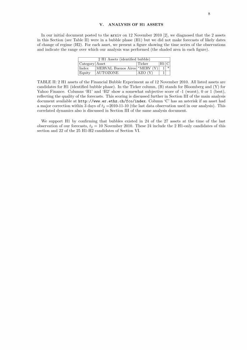
V. ANALYSIS OF H1 ASSETS
In our initial document posted to the arxiv on 12 November 2010 [2], we diagnosed that the 2 assetsin this Section (see Table II) were in a bubble phase (H1) but we did not make forecasts of likely datesof change of regime (H2). For each asset, we present a figure showing the time series of the observationsand indicate the range over which our analysis was performed (the shaded area in each figure).
2 H1 Assets (identified bubble)Category Asset Ticker H1 CIndex MERVAL Buenos Aires ^MERV (Y) 1 *Equity AUTOZONE AZO (Y) 1
TABLE II: 2 H1 assets of the Financial Bubble Experiment as of 12 November 2010. All listed assets arecandidates for H1 (identified bubble phase). In the Ticker column, (B) stands for Bloomberg and (Y) forYahoo Finance. Columns ‘H1’ and ‘H2’ show a somewhat subjective score of -1 (worst), 0 or 1 (best),reflecting the quality of the forecasts. This scoring is discussed further in Section III of the main analysisdocument available at http://www.er.ethz.ch/fco/index. Column ‘C’ has an asterisk if an asset hada major correction within 3 days of t2 =2010-11-10 (the last data observation used in our analysis). Thiscorrelated dynamics also is discussed in Section III of the same analysis document.
We support H1 by confirming that bubbles existed in 24 of the 27 assets at the time of the lastobservation of our forecasts, t2 = 10 November 2010. These 24 include the 2 H1-only candidates of thissection and 22 of the 25 H1-H2 candidates of Section VI.
9
A. H1 Indexes
1. MERVAL Buenos Aires
H1: 1
2010/02 2010/05 2010/08 2010/11 2011/02 2011/05date
2400
3000
3600
pric
e
last obs. price: 3311.0
last
obs
.: 20
10-1
1-10
dd1 (before t2): 18% / 47 daysdd2 (in quantiles): 4.2% / 7 days
dd3 (after quantiles): 13% / 55 daysdd2 / dd1 = 0.2dd2 / dd3 = 0.3
MERV - AR - drawdown
Observed prices
FIG. 1.
2010/02 2010/05 2010/08 2010/11 2011/02 2011/05date
2400
3000
3600
pric
e
last obs. price: 3311.0
last
obs
.: 20
10-1
1-10
MERV - AR - frac. up days in 60 day window
Observed prices
0.2
0.3
0.4
0.5
0.6
0.7
0.8fra
ctio
n up
day
s in
60
day
runn
ing
win
dow
frac. up days in 60 day window
FIG. 2.

10
2010/02 2010/05 2010/08 2010/11 2011/02 2011/05date
2400
3000
3600
pric
e
last obs. price: 3311.0
last
obs
.: 20
10-1
1-10
MERV - AR - Sav. Gol.
Observed prices
0.008
0.006
0.004
0.002
0.000
0.002
0.004
0.006
0.008
1st derivative, past and future60 smoothing points, polynomial order 3
FIG. 3.

11
B. H1 Equities
1. AUTOZONE
H1: 1
2010/03 2010/06 2010/09 2010/12 2011/03 2011/06date
150
200
250
pric
e
last obs. price: 248.9
last
obs
.: 20
10-1
1-10
dd1 (before t2): 5.7% / 4 daysdd2 (in quantiles): 9.9% / 7 days
dd3 (after quantiles): 4.7% / 7 daysdd2 / dd1 = 1.7dd2 / dd3 = 2.1
AZO - US - drawdown
Observed prices
FIG. 4.
2010/03 2010/06 2010/09 2010/12 2011/03 2011/06date
150
200
250
pric
e
last obs. price: 248.9
last
obs
.: 20
10-1
1-10
AZO - US - frac. up days in 60 day window
Observed prices
0.2
0.3
0.4
0.5
0.6
0.7
0.8fra
ctio
n up
day
s in
60
day
runn
ing
win
dow
frac. up days in 60 day window
FIG. 5.

12
2010/03 2010/06 2010/09 2010/12 2011/03 2011/06date
150
200
250
pric
e
last obs. price: 248.9
last
obs
.: 20
10-1
1-10
AZO - US - Sav. Gol.
Observed prices
0.008
0.006
0.004
0.002
0.000
0.002
0.004
0.006
0.008
1st derivative, past and future60 smoothing points, polynomial order 3
FIG. 6.
13
VI. ANALYSIS OF H1 & H2 ASSETS
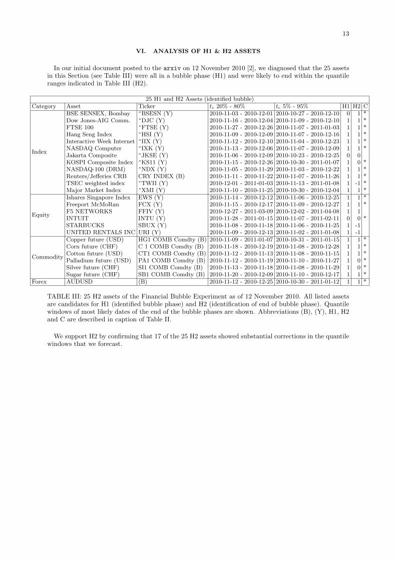
In our initial document posted to the arxiv on 12 November 2010 [2], we diagnosed that the 25 assetsin this Section (see Table III) were all in a bubble phase (H1) and were likely to end within the quantileranges indicated in Table III (H2).
25 H1 and H2 Assets (identified bubble)Category Asset Ticker tc 20% - 80% tc 5% - 95% H1 H2 C
Index
BSE SENSEX, Bombay ^BSESN (Y) 2010-11-03 - 2010-12-01 2010-10-27 - 2010-12-10 0 1 *Dow Jones-AIG Comm. ^DJC (Y) 2010-11-16 - 2010-12-04 2010-11-09 - 2010-12-10 1 1 *FTSE 100 ^FTSE (Y) 2010-11-27 - 2010-12-26 2010-11-07 - 2011-01-03 1 1 *Hang Seng Index ^HSI (Y) 2010-11-09 - 2010-12-09 2010-11-07 - 2010-12-16 1 1 *Interactive Week Internet ^IIX (Y) 2010-11-12 - 2010-12-10 2010-11-04 - 2010-12-23 1 1 *NASDAQ Computer ^IXK (Y) 2010-11-13 - 2010-12-06 2010-11-07 - 2010-12-09 1 1 *Jakarta Composite ^JKSE (Y) 2010-11-06 - 2010-12-09 2010-10-23 - 2010-12-25 0 0KOSPI Composite Index ^KS11 (Y) 2010-11-15 - 2010-12-26 2010-10-30 - 2011-01-07 1 0 *NASDAQ-100 (DRM) ^NDX (Y) 2010-11-05 - 2010-11-29 2010-11-03 - 2010-12-22 1 1 *Reuters/Jefferies CRB CRY INDEX (B) 2010-11-11 - 2010-11-22 2010-11-07 - 2010-11-26 1 1 *TSEC weighted index ^TWII (Y) 2010-12-01 - 2011-01-03 2010-11-13 - 2011-01-08 1 -1 *Major Market Index ^XMI (Y) 2010-11-10 - 2010-11-25 2010-10-30 - 2010-12-04 1 1 *
Equity
Ishares Singapore Index EWS (Y) 2010-11-14 - 2010-12-12 2010-11-06 - 2010-12-25 1 1 *Freeport McMoRan FCX (Y) 2010-11-15 - 2010-12-17 2010-11-09 - 2010-12-27 1 1 *F5 NETWORKS FFIV (Y) 2010-12-27 - 2011-03-09 2010-12-02 - 2011-04-08 1 1INTUIT INTU (Y) 2010-11-28 - 2011-01-15 2010-11-07 - 2011-02-11 0 0 *STARBUCKS SBUX (Y) 2010-11-08 - 2010-11-18 2010-11-06 - 2010-11-25 1 -1UNITED RENTALS INC URI (Y) 2010-11-09 - 2010-12-13 2010-11-02 - 2011-01-08 1 -1
Commodity
Copper future (USD) HG1 COMB Comdty (B) 2010-11-09 - 2011-01-07 2010-10-31 - 2011-01-15 1 1 *Corn future (CHF) C 1 COMB Comdty (B) 2010-11-18 - 2010-12-19 2010-11-08 - 2010-12-28 1 1 *Cotton future (USD) CT1 COMB Comdty (B) 2010-11-12 - 2010-11-13 2010-11-08 - 2010-11-15 1 1 *Palladium future (USD) PA1 COMB Comdty (B) 2010-11-12 - 2010-11-19 2010-11-10 - 2010-11-27 1 0 *Silver future (CHF) SI1 COMB Comdty (B) 2010-11-13 - 2010-11-18 2010-11-08 - 2010-11-29 1 0 *Sugar future (CHF) SB1 COMB Comdty (B) 2010-11-20 - 2010-12-09 2010-11-10 - 2010-12-17 1 1 *
Forex AUDUSD (B) 2010-11-12 - 2010-12-25 2010-10-30 - 2011-01-12 1 1 *
TABLE III: 25 H2 assets of the Financial Bubble Experiment as of 12 November 2010. All listed assetsare candidates for H1 (identified bubble phase) and H2 (identification of end of bubble phase). Quantilewindows of most likely dates of the end of the bubble phases are shown. Abbreviations (B), (Y), H1, H2and C are described in caption of Table II.
We support H2 by confirming that 17 of the 25 H2 assets showed substantial corrections in the quantilewindows that we forecast.
14
A. H1 & H2 Indexes
1. BSE SENSEX, Bombay
H1/H2: 0/1
2010/02 2010/05 2010/08 2010/11 2011/02 2011/05date
17500
20000
pric
e
last obs. price: 20875.7
last
obs
.: 20
10-1
1-10
dd1 (before t2): 11% / 48 daysdd2 (in quantiles): 9.3% / 21 days
dd3 (after quantiles): 16% / 38 daysdd2 / dd1 = 0.8dd2 / dd3 = 0.6
BSESN - IN - drawdown
Observed prices
FIG. 7.
2010/02 2010/05 2010/08 2010/11 2011/02 2011/05date
17500
20000
pric
e
last obs. price: 20875.7
last
obs
.: 20
10-1
1-10
BSESN - IN - frac. up days in 60 day window
Observed prices
0.2
0.3
0.4
0.5
0.6
0.7
0.8fra
ctio
n up
day
s in
60
day
runn
ing
win
dow
frac. up days in 60 day window
FIG. 8.
15
2010/02 2010/05 2010/08 2010/11 2011/02 2011/05date
17500
20000
pric
e
last obs. price: 20875.7la
st o
bs.:
2010
-11-
10
BSESN - IN - Sav. Gol.
Observed prices
0.008
0.006
0.004
0.002
0.000
0.002
0.004
0.006
0.008
1st derivative, past and future60 smoothing points, polynomial order 3
FIG. 9.

16
2. Dow Jones-AIG Commodity Index
H1/H2: 1/1
2010/02 2010/05 2010/08 2010/11 2011/02 2011/05date
125
150
175pr
ice
last obs. price: 154.2
last
obs
.: 20
10-1
1-10
dd1 (before t2): 11% / 50 daysdd2 (in quantiles): 8.5% / 8 days
dd3 (after quantiles): 7.2% / 11 daysdd2 / dd1 = 0.7dd2 / dd3 = 1.2
DJC - US - drawdown
Observed prices
FIG. 10.
2010/02 2010/05 2010/08 2010/11 2011/02 2011/05date
125
150
175
pric
e
last obs. price: 154.2
last
obs
.: 20
10-1
1-10
DJC - US - frac. up days in 60 day window
Observed prices
0.2
0.3
0.4
0.5
0.6
0.7
0.8fra
ctio
n up
day
s in
60
day
runn
ing
win
dow
frac. up days in 60 day window
FIG. 11.

17
2010/02 2010/05 2010/08 2010/11 2011/02 2011/05date
125
150
175
pric
e
last obs. price: 154.2
last
obs
.: 20
10-1
1-10
DJC - US - Sav. Gol.
Observed prices
0.008
0.006
0.004
0.002
0.000
0.002
0.004
0.006
0.008
1st derivative, past and future60 smoothing points, polynomial order 3
FIG. 12.
18
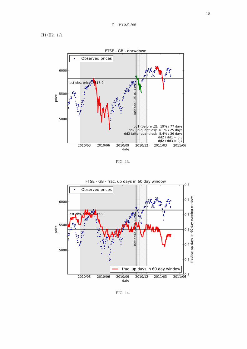
3. FTSE 100
H1/H2: 1/1
2010/03 2010/06 2010/09 2010/12 2011/03 2011/06date
5000
5500
6000
pric
e
last obs. price: 5816.9
last
obs
.: 20
10-1
1-10
dd1 (before t2): 19% / 77 daysdd2 (in quantiles): 6.1% / 25 days
dd3 (after quantiles): 8.4% / 36 daysdd2 / dd1 = 0.3dd2 / dd3 = 0.7
FTSE - GB - drawdown
Observed prices
FIG. 13.
2010/03 2010/06 2010/09 2010/12 2011/03 2011/06date
5000
5500
6000
pric
e
last obs. price: 5816.9
last
obs
.: 20
10-1
1-10
FTSE - GB - frac. up days in 60 day window
Observed prices
0.2
0.3
0.4
0.5
0.6
0.7
0.8fra
ctio
n up
day
s in
60
day
runn
ing
win
dow
frac. up days in 60 day window
FIG. 14.

19
2010/03 2010/06 2010/09 2010/12 2011/03 2011/06date
5000
5500
6000
pric
e
last obs. price: 5816.9
last
obs
.: 20
10-1
1-10
FTSE - GB - Sav. Gol.
Observed prices
0.008
0.006
0.004
0.002
0.000
0.002
0.004
0.006
0.008
1st derivative, past and future60 smoothing points, polynomial order 3
FIG. 15.

20
4. Hang Seng Index Hong Kong
H1/H2: 1/1
2010/02 2010/05 2010/08 2010/11 2011/02 2011/05date
20000
22500
25000
pric
e
last obs. price: 24500.6
last
obs
.: 20
10-1
1-10
dd1 (before t2): 15% / 46 daysdd2 (in quantiles): 9.6% / 38 days
dd3 (after quantiles): 9.1% / 57 daysdd2 / dd1 = 0.6dd2 / dd3 = 1.1
Hang Seng - CN - drawdown
Observed prices
FIG. 16.
2010/02 2010/05 2010/08 2010/11 2011/02 2011/05date
20000
22500
25000
pric
e
last obs. price: 24500.6
last
obs
.: 20
10-1
1-10
Hang Seng - CN - frac. up days in 60 day window
Observed prices
0.2
0.3
0.4
0.5
0.6
0.7
0.8fra
ctio
n up
day
s in
60
day
runn
ing
win
dow
frac. up days in 60 day window
FIG. 17.
21
2010/02 2010/05 2010/08 2010/11 2011/02 2011/05date
20000
22500
25000
pric
e
last obs. price: 24500.6
last
obs
.: 20
10-1
1-10
Hang Seng - CN - Sav. Gol.
Observed prices
0.008
0.006
0.004
0.002
0.000
0.002
0.004
0.006
0.008
1st derivative, past and future60 smoothing points, polynomial order 3
FIG. 18.

22
5. Interactive Week Internet Index
H1/H2: 1/1
2010/02 2010/05 2010/08 2010/11 2011/02date
240
280
320
pric
e
last obs. price: 312.7
last
obs
.: 20
10-1
1-10
dd1 (before t2): 17% / 78 daysdd2 (in quantiles): 6.4% / 6 days
dd3 (after quantiles): 4.3% / 3 daysdd2 / dd1 = 0.4dd2 / dd3 = 1.5
IIX - US - drawdown
Observed prices
FIG. 19.
2010/02 2010/05 2010/08 2010/11 2011/02date
240
280
320
pric
e
last obs. price: 312.7
last
obs
.: 20
10-1
1-10
IIX - US - frac. up days in 60 day window
Observed prices
0.2
0.3
0.4
0.5
0.6
0.7
0.8fra
ctio
n up
day
s in
60
day
runn
ing
win
dow
frac. up days in 60 day window
FIG. 20.

23
2010/02 2010/05 2010/08 2010/11 2011/02date
240
280
320
pric
e
last obs. price: 312.7la
st o
bs.:
2010
-11-
10
IIX - US - Sav. Gol.
Observed prices
0.008
0.006
0.004
0.002
0.000
0.002
0.004
0.006
0.008
1st derivative, past and future60 smoothing points, polynomial order 3
FIG. 21.

24
6. NASDAQ Computer
H1/H2: 1/1
2010/02 2010/05 2010/08 2010/11 2011/02 2011/05date
1200
1400
pric
e
last obs. price: 1336.0
last
obs
.: 20
10-1
1-10
dd1 (before t2): 19% / 70 daysdd2 (in quantiles): 4.8% / 8 days
dd3 (after quantiles): 9.7% / 27 daysdd2 / dd1 = 0.2dd2 / dd3 = 0.5
IXK - US - drawdown
Observed prices
FIG. 22.
2010/02 2010/05 2010/08 2010/11 2011/02 2011/05date
1200
1400
pric
e
last obs. price: 1336.0
last
obs
.: 20
10-1
1-10
IXK - US - frac. up days in 60 day window
Observed prices
0.2
0.3
0.4
0.5
0.6
0.7
0.8fra
ctio
n up
day
s in
60
day
runn
ing
win
dow
frac. up days in 60 day window
FIG. 23.

25
2010/02 2010/05 2010/08 2010/11 2011/02 2011/05date
1200
1400
pric
e
last obs. price: 1336.0
last
obs
.: 20
10-1
1-10
IXK - US - Sav. Gol.
Observed prices
0.008
0.006
0.004
0.002
0.000
0.002
0.004
0.006
0.008
1st derivative, past and future60 smoothing points, polynomial order 3
FIG. 24.

26
7. Jakarta Composite
H1/H2: 0/0
2009/06 2009/12 2010/06 2010/12 2011/06date
1600
2400
3200
pric
elast obs. price: 3757.0
last
obs
.: 20
10-1
1-10
dd1 (before t2): 16% / 25 daysdd2 (in quantiles): 6.2% / 20 days
dd3 (after quantiles): 12% / 19 daysdd2 / dd1 = 0.4dd2 / dd3 = 0.5
JKSE - ID - drawdown
Observed prices
FIG. 25.
2009/06 2009/12 2010/06 2010/12 2011/06date
1600
2400
3200
pric
e
last obs. price: 3757.0
last
obs
.: 20
10-1
1-10
JKSE - ID - frac. up days in 60 day window
Observed prices
0.2
0.3
0.4
0.5
0.6
0.7
0.8fra
ctio
n up
day
s in
60
day
runn
ing
win
dow
frac. up days in 60 day window
FIG. 26.

27
2009/06 2009/12 2010/06 2010/12 2011/06date
1600
2400
3200
pric
e
last obs. price: 3757.0
last
obs
.: 20
10-1
1-10
JKSE - ID - Sav. Gol.
Observed prices
0.008
0.006
0.004
0.002
0.000
0.002
0.004
0.006
0.008
1st derivative, past and future60 smoothing points, polynomial order 3
FIG. 27.
28
8. KOSPI Composite Index, Seoul
H1/H2: 1/0
2010/02 2010/05 2010/08 2010/11 2011/02 2011/05date
1500
1800
2100
pric
e
last obs. price: 1967.8
last
obs
.: 20
10-1
1-10
dd1 (before t2): 11% / 29 daysdd2 (in quantiles): 3.7% / 19 days
dd3 (after quantiles): 9.5% / 55 daysdd2 / dd1 = 0.3dd2 / dd3 = 0.4
KS11 - KR - drawdown
Observed prices
FIG. 28.
2010/02 2010/05 2010/08 2010/11 2011/02 2011/05date
1500
1800
2100
pric
e
last obs. price: 1967.8
last
obs
.: 20
10-1
1-10
KS11 - KR - frac. up days in 60 day window
Observed prices
0.2
0.3
0.4
0.5
0.6
0.7
0.8fra
ctio
n up
day
s in
60
day
runn
ing
win
dow
frac. up days in 60 day window
FIG. 29.
29
2010/02 2010/05 2010/08 2010/11 2011/02 2011/05date
1500
1800
2100
pric
e
last obs. price: 1967.8
last
obs
.: 20
10-1
1-10
KS11 - KR - Sav. Gol.
Observed prices
0.008
0.006
0.004
0.002
0.000
0.002
0.004
0.006
0.008
1st derivative, past and future60 smoothing points, polynomial order 3
FIG. 30.

30
9. NASDAQ-100 (DRM)
H1/H2: 1/1
2010/02 2010/05 2010/08 2010/11 2011/02 2011/05date
1800
2100
2400
pric
e
last obs. price: 2187.7
last
obs
.: 20
10-1
1-10
dd1 (before t2): 17% / 70 daysdd2 (in quantiles): 4.5% / 8 days
dd3 (after quantiles): 8.5% / 28 daysdd2 / dd1 = 0.3dd2 / dd3 = 0.5
NDX - US - drawdown
Observed prices
FIG. 31.
2010/02 2010/05 2010/08 2010/11 2011/02 2011/05date
1800
2100
2400
pric
e
last obs. price: 2187.7
last
obs
.: 20
10-1
1-10
NDX - US - frac. up days in 60 day window
Observed prices
0.2
0.3
0.4
0.5
0.6
0.7
0.8fra
ctio
n up
day
s in
60
day
runn
ing
win
dow
frac. up days in 60 day window
FIG. 32.

31
2010/02 2010/05 2010/08 2010/11 2011/02 2011/05date
1800
2100
2400
pric
e
last obs. price: 2187.7
last
obs
.: 20
10-1
1-10
NDX - US - Sav. Gol.
Observed prices
0.008
0.006
0.004
0.002
0.000
0.002
0.004
0.006
0.008
1st derivative, past and future60 smoothing points, polynomial order 3
FIG. 33.

32
10. Reuters/Jefferies CRB index
H1/H2: 1/1
2010/02 2010/05 2010/08 2010/11 2011/02 2011/05date
250
300
350
pric
e last obs. price: 317.1
last
obs
.: 20
10-1
1-10
dd1 (before t2): 11% / 41 daysdd2 (in quantiles): 7.7% / 8 days
dd3 (after quantiles): 7.1% / 8 daysdd2 / dd1 = 0.7dd2 / dd3 = 1.1
RJ CRB - US - drawdown
Observed prices
FIG. 34.
2010/02 2010/05 2010/08 2010/11 2011/02 2011/05date
250
300
350
pric
e last obs. price: 317.1
last
obs
.: 20
10-1
1-10
RJ CRB - US - frac. up days in 60 day window
Observed prices
0.2
0.3
0.4
0.5
0.6
0.7
0.8fra
ctio
n up
day
s in
60
day
runn
ing
win
dow
frac. up days in 60 day window
FIG. 35.
33
2010/02 2010/05 2010/08 2010/11 2011/02 2011/05date
250
300
350
pric
e last obs. price: 317.1
last
obs
.: 20
10-1
1-10
RJ CRB - US - Sav. Gol.
Observed prices
0.008
0.006
0.004
0.002
0.000
0.002
0.004
0.006
0.008
1st derivative, past and future60 smoothing points, polynomial order 3
FIG. 36.

34
11. TSEC weighted index
H1/H2: 1/-1
2010/02 2010/05 2010/08 2010/11 2011/02 2011/05date
7000
8000
9000
pric
e
last obs. price: 8450.6
last
obs
.: 20
10-1
1-10
dd1 (before t2): 14% / 55 daysdd2 (in quantiles): 2.7% / 4 days
dd3 (after quantiles): 10% / 46 daysdd2 / dd1 = 0.2dd2 / dd3 = 0.3
TWII - TW - drawdown
Observed prices
FIG. 37.
2010/02 2010/05 2010/08 2010/11 2011/02 2011/05date
7000
8000
9000
pric
e
last obs. price: 8450.6
last
obs
.: 20
10-1
1-10
TWII - TW - frac. up days in 60 day window
Observed prices
0.2
0.3
0.4
0.5
0.6
0.7
0.8fra
ctio
n up
day
s in
60
day
runn
ing
win
dow
frac. up days in 60 day window
FIG. 38.

35
2010/02 2010/05 2010/08 2010/11 2011/02 2011/05date
7000
8000
9000
pric
e
last obs. price: 8450.6
last
obs
.: 20
10-1
1-10
TWII - TW - Sav. Gol.
Observed prices
0.008
0.006
0.004
0.002
0.000
0.002
0.004
0.006
0.008
1st derivative, past and future60 smoothing points, polynomial order 3
FIG. 39.

36
12. Major Market Index
H1/H2: 1/1
2010/02 2010/05 2010/08 2010/11 2011/02date
1050
1200
1350
pric
e
last obs. price: 1245.2
last
obs
.: 20
10-1
1-10
dd1 (before t2): 14% / 70 daysdd2 (in quantiles): 3.9% / 25 days
dd3 (after quantiles): 1.7% / 4 daysdd2 / dd1 = 0.3dd2 / dd3 = 2.3
XMI - US - drawdown
Observed prices
FIG. 40.
2010/02 2010/05 2010/08 2010/11 2011/02date
1050
1200
1350
pric
e
last obs. price: 1245.2
last
obs
.: 20
10-1
1-10
XMI - US - frac. up days in 60 day window
Observed prices
0.2
0.3
0.4
0.5
0.6
0.7
0.8fra
ctio
n up
day
s in
60
day
runn
ing
win
dow
frac. up days in 60 day window
FIG. 41.
37
2010/02 2010/05 2010/08 2010/11 2011/02date
1050
1200
1350
pric
e
last obs. price: 1245.2
last
obs
.: 20
10-1
1-10
XMI - US - Sav. Gol.
Observed prices
0.008
0.006
0.004
0.002
0.000
0.002
0.004
0.006
0.008
1st derivative, past and future60 smoothing points, polynomial order 3
FIG. 42.
38
B. H1 & H2 Equities
1. Ishares Singapore Index
H1/H2: 1/1
2010/02 2010/05 2010/08 2010/11 2011/02 2011/05date
10
12
14
pric
e
last obs. price: 14.0
last
obs
.: 20
10-1
1-10
dd1 (before t2): 13% / 42 daysdd2 (in quantiles): 8.2% / 14 days
dd3 (after quantiles): 10% / 63 daysdd2 / dd1 = 0.6dd2 / dd3 = 0.8
EWS - US - drawdown
Observed prices
FIG. 43.
2010/02 2010/05 2010/08 2010/11 2011/02 2011/05date
10
12
14
pric
e
last obs. price: 14.0
last
obs
.: 20
10-1
1-10
EWS - US - frac. up days in 60 day window
Observed prices
0.2
0.3
0.4
0.5
0.6
0.7
0.8fra
ctio
n up
day
s in
60
day
runn
ing
win
dow
frac. up days in 60 day window
FIG. 44.

39
2010/02 2010/05 2010/08 2010/11 2011/02 2011/05date
10
12
14
pric
e
last obs. price: 14.0la
st o
bs.:
2010
-11-
10
EWS - US - Sav. Gol.
Observed prices
0.008
0.006
0.004
0.002
0.000
0.002
0.004
0.006
0.008
1st derivative, past and future60 smoothing points, polynomial order 3
FIG. 45.

40
2. Freeport McMoRan Copper & Gold
H1/H2: 1/1
2010/03 2010/06 2010/09 2010/12 2011/03 2011/06date
30
40
50
60pr
ice
last obs. price: 52.0
last
obs
.: 20
10-1
1-10
dd1 (before t2): 40% / 86 daysdd2 (in quantiles): 10% / 6 days
dd3 (after quantiles): 24% / 57 daysdd2 / dd1 = 0.3dd2 / dd3 = 0.4
FCX - US - drawdown
Observed prices
FIG. 46.
2010/03 2010/06 2010/09 2010/12 2011/03 2011/06date
30
40
50
60
pric
e
last obs. price: 52.0
last
obs
.: 20
10-1
1-10
FCX - US - frac. up days in 60 day window
Observed prices
0.2
0.3
0.4
0.5
0.6
0.7
0.8fra
ctio
n up
day
s in
60
day
runn
ing
win
dow
frac. up days in 60 day window
FIG. 47.
41
2010/03 2010/06 2010/09 2010/12 2011/03 2011/06date
30
40
50
60
pric
e
last obs. price: 52.0
last
obs
.: 20
10-1
1-10
FCX - US - Sav. Gol.
Observed prices
0.008
0.006
0.004
0.002
0.000
0.002
0.004
0.006
0.008
1st derivative, past and future60 smoothing points, polynomial order 3
FIG. 48.

42
3. F5 NETWORKS
H1/H2: 1/1
2009/06 2009/12 2010/06 2010/12 2011/06date
40
80
120pr
ice
last obs. price: 122.9
last
obs
.: 20
10-1
1-10
dd1 (before t2): 20% / 14 daysdd2 (in quantiles): 45% / 67 days
dd3 (after quantiles): 0.0% / 0 daysdd2 / dd1 = 2.2dd2 / dd3 = 0.0
FFIV - US - drawdown
Observed prices
FIG. 49.
2009/06 2009/12 2010/06 2010/12 2011/06date
40
80
120
pric
e
last obs. price: 122.9
last
obs
.: 20
10-1
1-10
FFIV - US - frac. up days in 60 day window
Observed prices
0.2
0.3
0.4
0.5
0.6
0.7
0.8fra
ctio
n up
day
s in
60
day
runn
ing
win
dow
frac. up days in 60 day window
FIG. 50.
43
2009/06 2009/12 2010/06 2010/12 2011/06date
40
80
120
pric
e
last obs. price: 122.9
last
obs
.: 20
10-1
1-10
FFIV - US - Sav. Gol.
Observed prices
0.008
0.006
0.004
0.002
0.000
0.002
0.004
0.006
0.008
1st derivative, past and future60 smoothing points, polynomial order 3
FIG. 51.
44
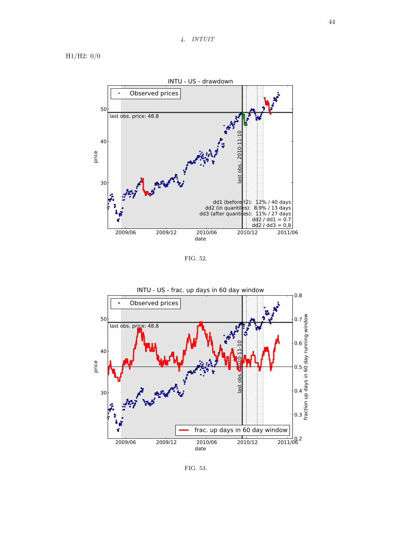
4. INTUIT
H1/H2: 0/0
2009/06 2009/12 2010/06 2010/12 2011/06date
30
40
50
pric
e
last obs. price: 48.8
last
obs
.: 20
10-1
1-10
dd1 (before t2): 12% / 40 daysdd2 (in quantiles): 8.9% / 13 days
dd3 (after quantiles): 11% / 27 daysdd2 / dd1 = 0.7dd2 / dd3 = 0.8
INTU - US - drawdown
Observed prices
FIG. 52.
2009/06 2009/12 2010/06 2010/12 2011/06date
30
40
50
pric
e
last obs. price: 48.8
last
obs
.: 20
10-1
1-10
INTU - US - frac. up days in 60 day window
Observed prices
0.2
0.3
0.4
0.5
0.6
0.7
0.8fra
ctio
n up
day
s in
60
day
runn
ing
win
dow
frac. up days in 60 day window
FIG. 53.

45
2009/06 2009/12 2010/06 2010/12 2011/06date
30
40
50
pric
e
last obs. price: 48.8
last
obs
.: 20
10-1
1-10
INTU - US - Sav. Gol.
Observed prices
0.008
0.006
0.004
0.002
0.000
0.002
0.004
0.006
0.008
1st derivative, past and future60 smoothing points, polynomial order 3
FIG. 54.
46
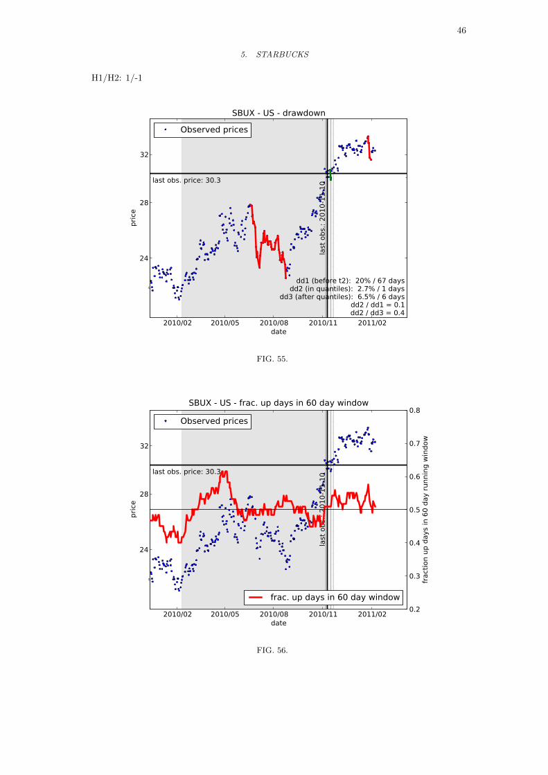
5. STARBUCKS
H1/H2: 1/-1
2010/02 2010/05 2010/08 2010/11 2011/02date
24
28
32
pric
e
last obs. price: 30.3
last
obs
.: 20
10-1
1-10
dd1 (before t2): 20% / 67 daysdd2 (in quantiles): 2.7% / 1 days
dd3 (after quantiles): 6.5% / 6 daysdd2 / dd1 = 0.1dd2 / dd3 = 0.4
SBUX - US - drawdown
Observed prices
FIG. 55.
2010/02 2010/05 2010/08 2010/11 2011/02date
24
28
32
pric
e
last obs. price: 30.3
last
obs
.: 20
10-1
1-10
SBUX - US - frac. up days in 60 day window
Observed prices
0.2
0.3
0.4
0.5
0.6
0.7
0.8fra
ctio
n up
day
s in
60
day
runn
ing
win
dow
frac. up days in 60 day window
FIG. 56.

47
2010/02 2010/05 2010/08 2010/11 2011/02date
24
28
32
pric
e
last obs. price: 30.3la
st o
bs.:
2010
-11-
10
SBUX - US - Sav. Gol.
Observed prices
0.008
0.006
0.004
0.002
0.000
0.002
0.004
0.006
0.008
1st derivative, past and future60 smoothing points, polynomial order 3
FIG. 57.

48
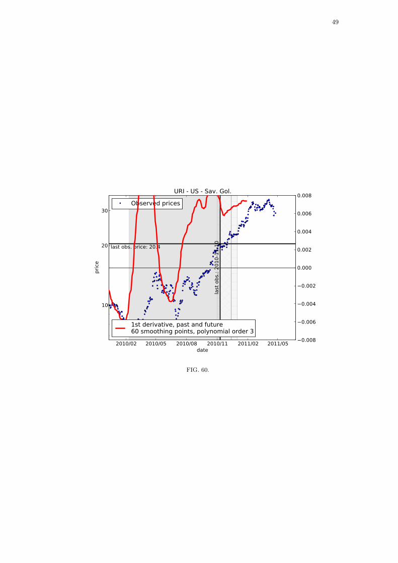
6. UNITED RENTALS INC
H1/H2: 1/-1
2010/02 2010/05 2010/08 2010/11 2011/02 2011/05date
10
20
30pr
ice
last obs. price: 20.4
last
obs
.: 20
10-1
1-10
dd1 (before t2): 56% / 64 daysdd2 (in quantiles): 6.9% / 5 days
dd3 (after quantiles): 18% / 15 daysdd2 / dd1 = 0.1dd2 / dd3 = 0.4
URI - US - drawdown
Observed prices
FIG. 58.
2010/02 2010/05 2010/08 2010/11 2011/02 2011/05date
10
20
30
pric
e
last obs. price: 20.4
last
obs
.: 20
10-1
1-10
URI - US - frac. up days in 60 day window
Observed prices
0.2
0.3
0.4
0.5
0.6
0.7
0.8fra
ctio
n up
day
s in
60
day
runn
ing
win
dow
frac. up days in 60 day window
FIG. 59.
49
2010/02 2010/05 2010/08 2010/11 2011/02 2011/05date
10
20
30
pric
e
last obs. price: 20.4
last
obs
.: 20
10-1
1-10
URI - US - Sav. Gol.
Observed prices
0.008
0.006
0.004
0.002
0.000
0.002
0.004
0.006
0.008
1st derivative, past and future60 smoothing points, polynomial order 3
FIG. 60.

50
C. H1 & H2 Commodities
1. Copper future (USD)
H1/H2: 1/1
2010/02 2010/05 2010/08 2010/11 2011/02 2011/05date
3.2
4.0
4.8
pric
e
last obs. price: 4.0
last
obs
.: 20
10-1
1-10
dd1 (before t2): 27% / 63 daysdd2 (in quantiles): 8.8% / 14 days
dd3 (after quantiles): 11% / 29 daysdd2 / dd1 = 0.3dd2 / dd3 = 0.8
Copper future - USD - drawdown
Observed prices
FIG. 61.
2010/02 2010/05 2010/08 2010/11 2011/02 2011/05date
3.2
4.0
4.8
pric
e
last obs. price: 4.0
last
obs
.: 20
10-1
1-10
Copper future - USD - frac. up days in 60 day window
Observed prices
0.2
0.3
0.4
0.5
0.6
0.7
0.8fra
ctio
n up
day
s in
60
day
runn
ing
win
dow
frac. up days in 60 day window
FIG. 62.

51
2010/02 2010/05 2010/08 2010/11 2011/02 2011/05date
3.2
4.0
4.8
pric
e
last obs. price: 4.0
last
obs
.: 20
10-1
1-10
Copper future - USD - Sav. Gol.
Observed prices
0.008
0.006
0.004
0.002
0.000
0.002
0.004
0.006
0.008
1st derivative, past and future60 smoothing points, polynomial order 3
FIG. 63.

52
2. Corn future (CHF)
H1/H2: 1/1
2010/02 2010/05 2010/08 2010/11 2011/02 2011/05date
4.5
6.0
pric
e
last obs. price: 5.5
last
obs
.: 20
10-1
1-10
dd1 (before t2): 20% / 33 daysdd2 (in quantiles): 10.0% / 14 days
dd3 (after quantiles): 20% / 33 daysdd2 / dd1 = 0.5dd2 / dd3 = 0.5
Corn future - CHF - drawdown
Observed prices
FIG. 64.
2010/02 2010/05 2010/08 2010/11 2011/02 2011/05date
4.5
6.0
pric
e
last obs. price: 5.5
last
obs
.: 20
10-1
1-10
Corn future - CHF - frac. up days in 60 day window
Observed prices
0.2
0.3
0.4
0.5
0.6
0.7
0.8fra
ctio
n up
day
s in
60
day
runn
ing
win
dow
frac. up days in 60 day window
FIG. 65.

53
2010/02 2010/05 2010/08 2010/11 2011/02 2011/05date
4.5
6.0
pric
e
last obs. price: 5.5
last
obs
.: 20
10-1
1-10
Corn future - CHF - Sav. Gol.
Observed prices
0.008
0.006
0.004
0.002
0.000
0.002
0.004
0.006
0.008
1st derivative, past and future60 smoothing points, polynomial order 3
FIG. 66.

54
3. Cotton future (USD)
H1/H2: 1/1
2010/02 2010/05 2010/08 2010/11 2011/02 2011/05date
1.0
1.5
2.0pr
ice
last obs. price: 1.5
last
obs
.: 20
10-1
1-10
dd1 (before t2): 9.3% / 17 daysdd2 (in quantiles): 8.6% / 6 days
dd3 (after quantiles): 20% / 8 daysdd2 / dd1 = 0.9dd2 / dd3 = 0.4
Cotton future - USD - drawdown
Observed prices
FIG. 67.
2010/02 2010/05 2010/08 2010/11 2011/02 2011/05date
1.0
1.5
2.0
pric
e
last obs. price: 1.5
last
obs
.: 20
10-1
1-10
Cotton future - USD - frac. up days in 60 day window
Observed prices
0.2
0.3
0.4
0.5
0.6
0.7
0.8fra
ctio
n up
day
s in
60
day
runn
ing
win
dow
frac. up days in 60 day window
FIG. 68.

55
2010/02 2010/05 2010/08 2010/11 2011/02 2011/05date
1.0
1.5
2.0
pric
e
last obs. price: 1.5
last
obs
.: 20
10-1
1-10
Cotton future - USD - Sav. Gol.
Observed prices
0.008
0.006
0.004
0.002
0.000
0.002
0.004
0.006
0.008
1st derivative, past and future60 smoothing points, polynomial order 3
FIG. 69.
56
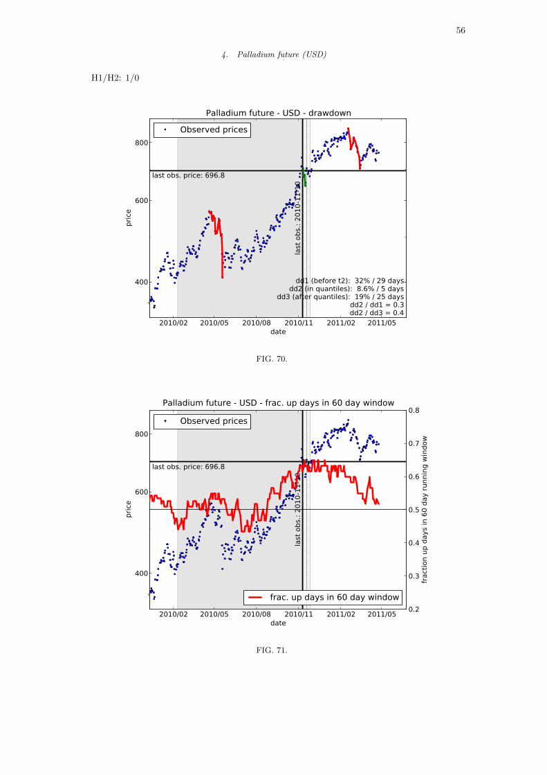
4. Palladium future (USD)
H1/H2: 1/0
2010/02 2010/05 2010/08 2010/11 2011/02 2011/05date
400
600
800
pric
e
last obs. price: 696.8
last
obs
.: 20
10-1
1-10
dd1 (before t2): 32% / 29 daysdd2 (in quantiles): 8.6% / 5 days
dd3 (after quantiles): 19% / 25 daysdd2 / dd1 = 0.3dd2 / dd3 = 0.4
Palladium future - USD - drawdown
Observed prices
FIG. 70.
2010/02 2010/05 2010/08 2010/11 2011/02 2011/05date
400
600
800
pric
e
last obs. price: 696.8
last
obs
.: 20
10-1
1-10
Palladium future - USD - frac. up days in 60 day window
Observed prices
0.2
0.3
0.4
0.5
0.6
0.7
0.8fra
ctio
n up
day
s in
60
day
runn
ing
win
dow
frac. up days in 60 day window
FIG. 71.

57
2010/02 2010/05 2010/08 2010/11 2011/02 2011/05date
400
600
800
pric
e
last obs. price: 696.8
last
obs
.: 20
10-1
1-10
Palladium future - USD - Sav. Gol.
Observed prices
0.008
0.006
0.004
0.002
0.000
0.002
0.004
0.006
0.008
1st derivative, past and future60 smoothing points, polynomial order 3
FIG. 72.

58
5. Silver future (CHF)
H1/H2: 1/0
2010/02 2010/05 2010/08 2010/11 2011/02 2011/05date
20
30
40pr
ice
last obs. price: 26.2
last
obs
.: 20
10-1
1-10
dd1 (before t2): 17% / 78 daysdd2 (in quantiles): 10% / 7 days
dd3 (after quantiles): 14% / 49 daysdd2 / dd1 = 0.6dd2 / dd3 = 0.7
Silver future - CHF - drawdown
Observed prices
FIG. 73.
2010/02 2010/05 2010/08 2010/11 2011/02 2011/05date
20
30
40
pric
e
last obs. price: 26.2
last
obs
.: 20
10-1
1-10
Silver future - CHF - frac. up days in 60 day window
Observed prices
0.2
0.3
0.4
0.5
0.6
0.7
0.8fra
ctio
n up
day
s in
60
day
runn
ing
win
dow
frac. up days in 60 day window
FIG. 74.

59
2010/02 2010/05 2010/08 2010/11 2011/02 2011/05date
20
30
40
pric
e
last obs. price: 26.2
last
obs
.: 20
10-1
1-10
Silver future - CHF - Sav. Gol.
Observed prices
0.008
0.006
0.004
0.002
0.000
0.002
0.004
0.006
0.008
1st derivative, past and future60 smoothing points, polynomial order 3
FIG. 75.

60
6. Sugar future (CHF)
H1/H2: 1/1
2010/02 2010/05 2010/08 2010/11 2011/02 2011/05date
0.18
0.24
0.30
pric
e
last obs. price: 0.3
last
obs
.: 20
10-1
1-10
dd1 (before t2): 66% / 84 daysdd2 (in quantiles): 21% / 2 days
dd3 (after quantiles): 42% / 71 daysdd2 / dd1 = 0.3dd2 / dd3 = 0.5
Sugar future - CHF - drawdown
Observed prices
FIG. 76.
2010/02 2010/05 2010/08 2010/11 2011/02 2011/05date
0.18
0.24
0.30
pric
e
last obs. price: 0.3
last
obs
.: 20
10-1
1-10
Sugar future - CHF - frac. up days in 60 day window
Observed prices
0.2
0.3
0.4
0.5
0.6
0.7
0.8fra
ctio
n up
day
s in
60
day
runn
ing
win
dow
frac. up days in 60 day window
FIG. 77.

61
2010/02 2010/05 2010/08 2010/11 2011/02 2011/05date
0.18
0.24
0.30
pric
e
last obs. price: 0.3la
st o
bs.:
2010
-11-
10
Sugar future - CHF - Sav. Gol.
Observed prices
0.008
0.006
0.004
0.002
0.000
0.002
0.004
0.006
0.008
1st derivative, past and future60 smoothing points, polynomial order 3
FIG. 78.
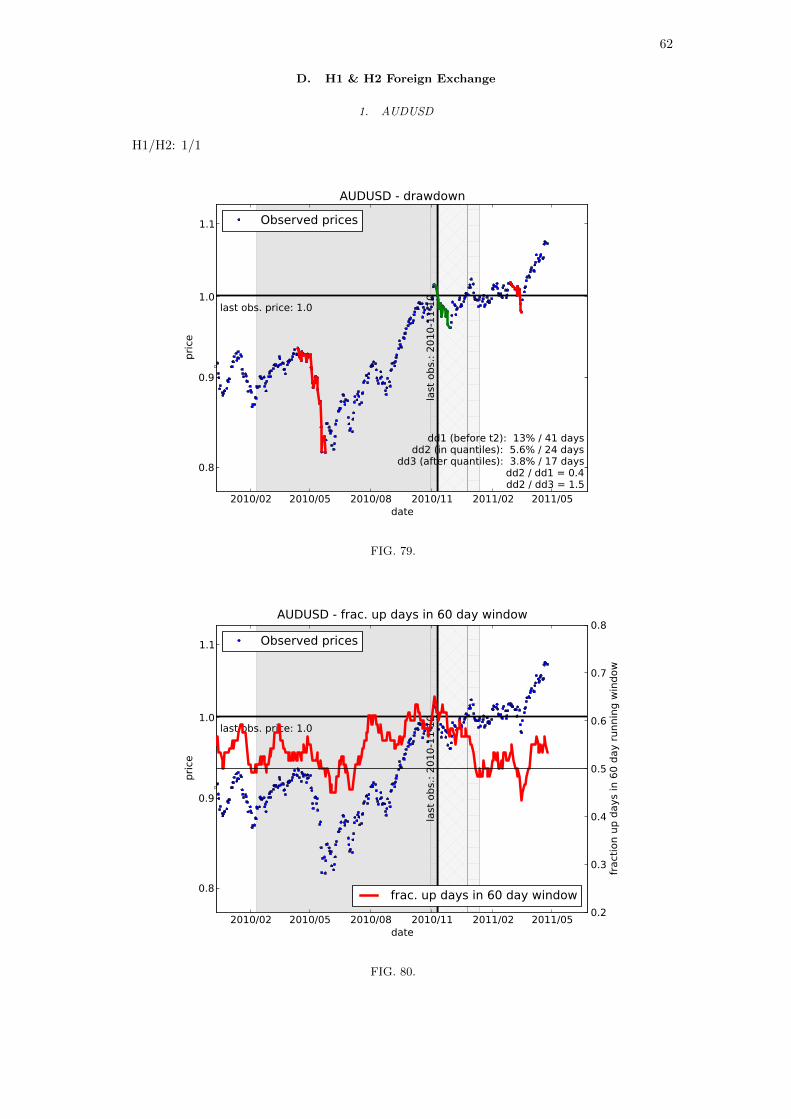
62
D. H1 & H2 Foreign Exchange
1. AUDUSD
H1/H2: 1/1
2010/02 2010/05 2010/08 2010/11 2011/02 2011/05date
0.8
0.9
1.0
1.1
pric
e
last obs. price: 1.0
last
obs
.: 20
10-1
1-10
dd1 (before t2): 13% / 41 daysdd2 (in quantiles): 5.6% / 24 days
dd3 (after quantiles): 3.8% / 17 daysdd2 / dd1 = 0.4dd2 / dd3 = 1.5
AUDUSD - drawdown
Observed prices
FIG. 79.
2010/02 2010/05 2010/08 2010/11 2011/02 2011/05date
0.8
0.9
1.0
1.1
pric
e
last obs. price: 1.0
last
obs
.: 20
10-1
1-10
AUDUSD - frac. up days in 60 day window
Observed prices
0.2
0.3
0.4
0.5
0.6
0.7
0.8fra
ctio
n up
day
s in
60
day
runn
ing
win
dow
frac. up days in 60 day window
FIG. 80.
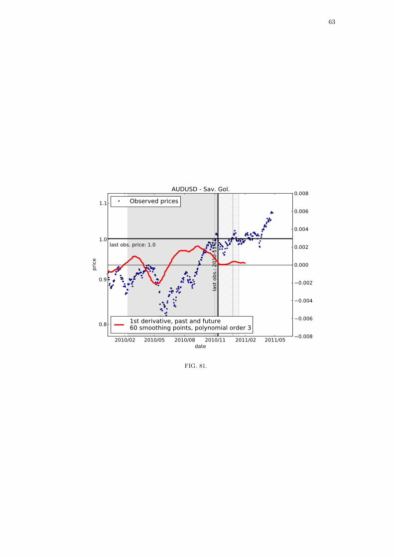
63
2010/02 2010/05 2010/08 2010/11 2011/02 2011/05date
0.8
0.9
1.0
1.1
pric
e
last obs. price: 1.0
last
obs
.: 20
10-1
1-10
AUDUSD - Sav. Gol.
Observed prices
0.008
0.006
0.004
0.002
0.000
0.002
0.004
0.006
0.008
1st derivative, past and future60 smoothing points, polynomial order 3
FIG. 81.

64
VII. STATE OF THE MARKET AT TIME OF ANALYSIS (NOVEMBER 2010)
Please see next page.

MERVAL The Argentinian Merval index is the most important index of the Buenos Aires stock exchange serving as a measure for Argentina’s business climate. In 2010 the Heritage Foundation Index of Economic Freedomi awarded Argentina only a 45 percent score for the factor "Investment Freedom" amid its uncertain creditor situation and doubts over contract and property rights. Argentina is experiencing high inflation and political uncertainties. In 2010, investors started to discuss concerns on a potential future default risk. The MERVAL index increased by 41 percent from September 1st to November 4th 2010.
Autozone (AZO) Autozone is an auto parts retailer. Investors recommend these industry stocks as recession proof, as in economically hard times consumers tend to delay new auto purchases, which in turn increases demand for do‐it‐yourself repairs. In September 2010, Autozone reported a 14 percent jump in fiscal Q4 earnings. Afterwards, the share price rose substantially higher.
BSESN BSE SENSEX, Bombay (Index) According to the Bombay Stock Exchange, the SENSEX index is the barometer of the Indian Capital Markets. India encourages foreign investment and provides export and tax incentives to foreign investors. Nevertheless, it regulates the industry sectors and conditions for foreign investments. India has been a hotspot for emerging market investors. With its large population and still developing markets it provides a substantial potential for further growth.
“The growth of the equity market in India has been phenomenal in the present decade. Right from early nineties, the stock market witnessed heightened activity in terms of various bull and bear runs. In the late nineties, the Indian market witnessed a huge frenzy in the 'TMT' sectors. More recently, real estate caught the fancy of the investors. SENSEX has captured all these happenings in the most judicious manner. One can identify the booms and busts of the Indian equity market through SENSEX. As the oldest index in the country, it provides the time series data over a fairly long period of time (from 1979 onwards). Small wonder, the SENSEX has become one of the most prominent brands in the country.” (bseindia.com) The SENSEX enjoyed an 18 percent rally from end of October to November 4, 2010.
The Dow Jones AIG Commodity Index The Dow Jones ‐ AIG Commodity Index is a benchmark for the commodity futures market. The index consists of a diversified portfolio of commodities composed of futures contracts on 19 physical commodities listed at U.S. exchanges and the London Metal Exchange. It tracks non‐related commodities such as energy, precious metals, livestock and grains with a weighting between 2 and 15 percent.
FTSE FTSE 100 (Index) The FTSE 100 index comprises the 100 most highly capitalized blue chip companies in the UK, representing approximately 81% of the UK market. It is used extensively as a basis for investment products, such as derivatives and exchange‐traded funds, listed at the London Stock Exchange. The index rose more than 12 percent from September to November, after it had been falling dramatically during the financial crisis of 2007‐2010 to a low of below 3,500. The FTSE 100 index recovery from the financial crisis took some set‐backs in 2010 amid the emergence of the European crisis.
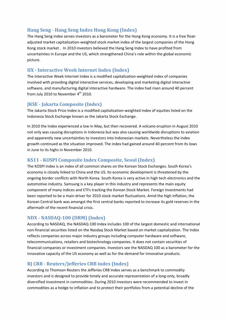
Hang Seng Hang Seng Index Hong Kong (Index) The Hang Seng index serves investors as a barometer for the Hong Kong economy. It is a free float‐adjusted market capitalization‐weighted stock market index of the largest companies of the Hong Kong stock market . In 2010 investors believed the Hang Seng Index to have profited from uncertainties in Europe and the US, which strengthened China’s role within the global economic picture.
IIX Interactive Week Internet Index (Index) The Interactive Week Internet Index is a modified capitalization‐weighted index of companies involved with providing digital interactive services, developing and marketing digital interactive software, and manufacturing digital interactive hardware. The index had risen around 40 percent from July 2010 to November 4th 2010.
JKSE Jakarta Composite (Index) The Jakarta Stock Price Index is a modified capitalization‐weighted index of equities listed on the Indonesia Stock Exchange known as the Jakarta Stock Exchange.
In 2010 the Index experienced a low in May, but then recovered. A volcano eruption in August 2010 not only was causing disruptions in Indonesia but was also causing worldwide disruptions to aviation and apparently new uncertainties to investors into Indonesian markets. Nevertheless the index growth continued as the situation improved. The index had gained around 40 percent from its lows in June to its highs in November 2010.
KS11 KOSPI Composite Index Composite, Seoul (Index) The KOSPI Index is an index of all common shares on the Korean Stock Exchanges. South Korea’s economy is closely linked to China and the US. Its economic development is threatened by the ongoing border conflicts with North Korea. South Korea is very active in high tech electronics and the automotive industry. Samsung is a key player in this industry and represents the main equity component of many indices and ETFs tracking the Korean Stock Market. Foreign investments had been reported to be a main driver for 2010 stock market fluctuations. Amid the high inflation, the Korean Central bank was amongst the first central banks reported to increase its gold reserves in the aftermath of the recent financial crisis.
NDX NASDAQ100 (DRM) (Index) According to NASDAQ, the NASDAQ‐100 Index includes 100 of the largest domestic and international non‐financial securities listed on the Nasdaq Stock Market based on market capitalization. The Index reflects companies across major industry groups including computer hardware and software, telecommunications, retailers and biotechnology companies. It does not contain securities of financial companies or investment companies. Investors see the NASDAQ 100 as a barometer for the innovative capacity of the US economy as well as for the demand for innovative products.
RJ CRB Reuters/Jefferies CRB index (Index) According to Thomson Reuters the Jefferies CRB Index serves as a benchmark to commodity investors and is designed to provide timely and accurate representation of a long‐only, broadly diversified investment in commodities. During 2010 investors were recommended to invest in commodities as a hedge to inflation and to protect their portfolios from a potential decline of the

USD. Other reasons for commodity investments were the ongoing economic recovery in the US and the continued growth of the Chinese economy.
TWII TSEC weighted index (Index) The TSEC Taiwan Technology Index is a market‐cap weighted index of stocks which are the technology sector members of the TW50 and TWMC indices. Taiwan’s economy is closely related to Asian economies and in 2010 Taiwan started to invest in mainland China.
XMI Major Market Index (Index) The NYSE Major Market Index is a price‐weighted index of 20 blue‐chip stocks representative of major US industrial corporations. The XMI rose by 13 percent from September to November 2010.
EWS Ishares Singapore Index (ETF) The iShares MSCI Singapore Index Fund is an exchange‐traded fund incorporated in the USA allowing investors to invest in a tool which corresponds to the performance to the MSCI Singapore Index. The Fund invests in a representative sample of index stocks using a "portfolio sampling" technique. EWS gained nearly 40 percent from July to November 2010.
FCX Freeport McMoRan Copper & Gold (Equity) Freeport is one of the world’s leading copper and gold producers. Freeport is often referred to as the “lowest cost” copper producer. In its guidance for 2010 Freeport reported an expected lower demand for copper in 2010 amid China growth concerns. After a significant reduction in debt, Moody’s raisedii Freeport’s bond rating from Junk to Baa3, after which the stock rose.
FFIV F5 NETWORKS (Equity) F5 Networks provides technology that optimizes the delivery of network‐based applications and the security, performance and availability of servers, data storage devices and other network resources. F5 Networks is a major supplier for many of the top 50 of the Fortune 500 companies, online video services and internet search companies.
Investors investing in F5 networks seemingly seek to benefit from increasing internet traffic and large corporations’ needs to optimize component utilization and traffic. Its fiscal Q3 2010 profit rose by 77.5% and in August 2010 F5 Networks announced it would provide “cloudbusting” solutions to its clients. Cloud Computing had become the technology buzz‐word in 2010.
INTU – INTUIT (Equity) Intuit Inc. is the provider of business and financial management solutions focused on small and medium‐sized businesses and consumers. It provides well known financial software applications such as Quicken and Quick books. In 2010 Intuit was ranked 94 on the Forbes top‐100 best companies to work for.
In August 2010 Intuit reported an 11 percent increase in revenues resulting in a 31 percent increased EPS in fiscal year 2010 compared to fiscal year 2009.
URI UNITED RENTALS INC (Equity) United Rentals is a world leading rental and leasing company. According to Reuters it offers approximately 2,900 classes of equipment for rent. Its main customers include construction and
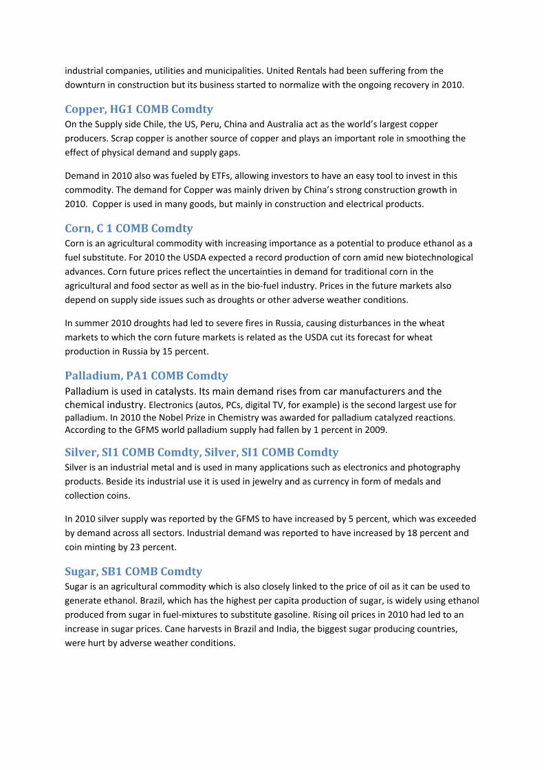
industrial companies, utilities and municipalities. United Rentals had been suffering from the downturn in construction but its business started to normalize with the ongoing recovery in 2010.
Copper, HG1 COMB Comdty On the Supply side Chile, the US, Peru, China and Australia act as the world’s largest copper producers. Scrap copper is another source of copper and plays an important role in smoothing the effect of physical demand and supply gaps.
Demand in 2010 also was fueled by ETFs, allowing investors to have an easy tool to invest in this commodity. The demand for Copper was mainly driven by China’s strong construction growth in 2010. Copper is used in many goods, but mainly in construction and electrical products.
Corn, C 1 COMB Comdty Corn is an agricultural commodity with increasing importance as a potential to produce ethanol as a fuel substitute. For 2010 the USDA expected a record production of corn amid new biotechnological advances. Corn future prices reflect the uncertainties in demand for traditional corn in the agricultural and food sector as well as in the bio‐fuel industry. Prices in the future markets also depend on supply side issues such as droughts or other adverse weather conditions.
In summer 2010 droughts had led to severe fires in Russia, causing disturbances in the wheat markets to which the corn future markets is related as the USDA cut its forecast for wheat production in Russia by 15 percent.
Palladium, PA1 COMB Comdty Palladium is used in catalysts. Its main demand rises from car manufacturers and the chemical industry. Electronics (autos, PCs, digital TV, for example) is the second largest use for palladium. In 2010 the Nobel Prize in Chemistry was awarded for palladium catalyzed reactions. According to the GFMS world palladium supply had fallen by 1 percent in 2009.
Silver, SI1 COMB Comdty, Silver, SI1 COMB Comdty Silver is an industrial metal and is used in many applications such as electronics and photography products. Beside its industrial use it is used in jewelry and as currency in form of medals and collection coins.
In 2010 silver supply was reported by the GFMS to have increased by 5 percent, which was exceeded by demand across all sectors. Industrial demand was reported to have increased by 18 percent and coin minting by 23 percent.
Sugar, SB1 COMB Comdty Sugar is an agricultural commodity which is also closely linked to the price of oil as it can be used to generate ethanol. Brazil, which has the highest per capita production of sugar, is widely using ethanol produced from sugar in fuel‐mixtures to substitute gasoline. Rising oil prices in 2010 had led to an increase in sugar prices. Cane harvests in Brazil and India, the biggest sugar producing countries, were hurt by adverse weather conditions.

The 2010 Market Situation For investors the year 2010 was the year of uncertainty and the start of strategic portfolio repositioning. After the dreadful emergence of the financial crisis in 2008, investors had experienced a fantastic stock market rebound in 2009 carried by low interest rates and capital injections by governments around the world. In 2010 those capital injections started to raise first concerns.
The aftermaths of the crisis manifested with the emergence of the Dubai World crisisiii in late 2009 and the European crisis in early 2010iv. While an immediate global system meltdown had been averted, there was contagion amongst sovereign states as a consequence.
World leaders had acted and taken unprecedented steps in 2008 after the Lehman collapse, by expanding and eventually bending the current regulation framework in order to avoid a breakdown of the global banking system. The primary effects had spanned from the US, where regulators decided on seizing large firms including AIG and GM and to inject large sums of money into the banking system under the TARP program, to other countries around the globe. Secondary effects led for example to an expectation of bank runs in Germany, which had ultimately to be avoided by providing guarantees, without legal parliamentary support as Germany’s former finance minister Peer Steinbrueck admitted during a public speech in early 2011v.
While those actions had not been questioned at the time of emergency, the public started to question in hindsight the validity and impact of those actions with the emergence of the sovereign debt crisis in 2010.
In 2010 the crisis started to raise concerns over Greece, Ireland and Portugal, which required another set of emergency regulations as a new threat to the financial system. This was a clear sign to investors that markets had not yet fully recovered and needed support beyond the current level of recovery. With the end of the FED’s QE program, discussions arose on the scope of QE2 and its future impactvi. Some investors anticipated a continuation of the dollar devaluation: “The U.S. has gotten itself into a bind. To emerge from this recession successfully over the long term, it will have no choice but to inflate its currency and monetize its debt and entitlement burden.”vii
Therefore expectations in Q4 2010 were either set to disappoint stock market or dollar investors and in the worst case, both.
Market’s anticipation of the FED’s QE2 Program in Q4 2010 When the FED issued its press releaseviii on its QE2 Program on 3rd of November 2011, it was no longer a large surprise to investors, but its scope and impact were discussed during the following weeks as an analysis of Google Trends indicates (picture 1).
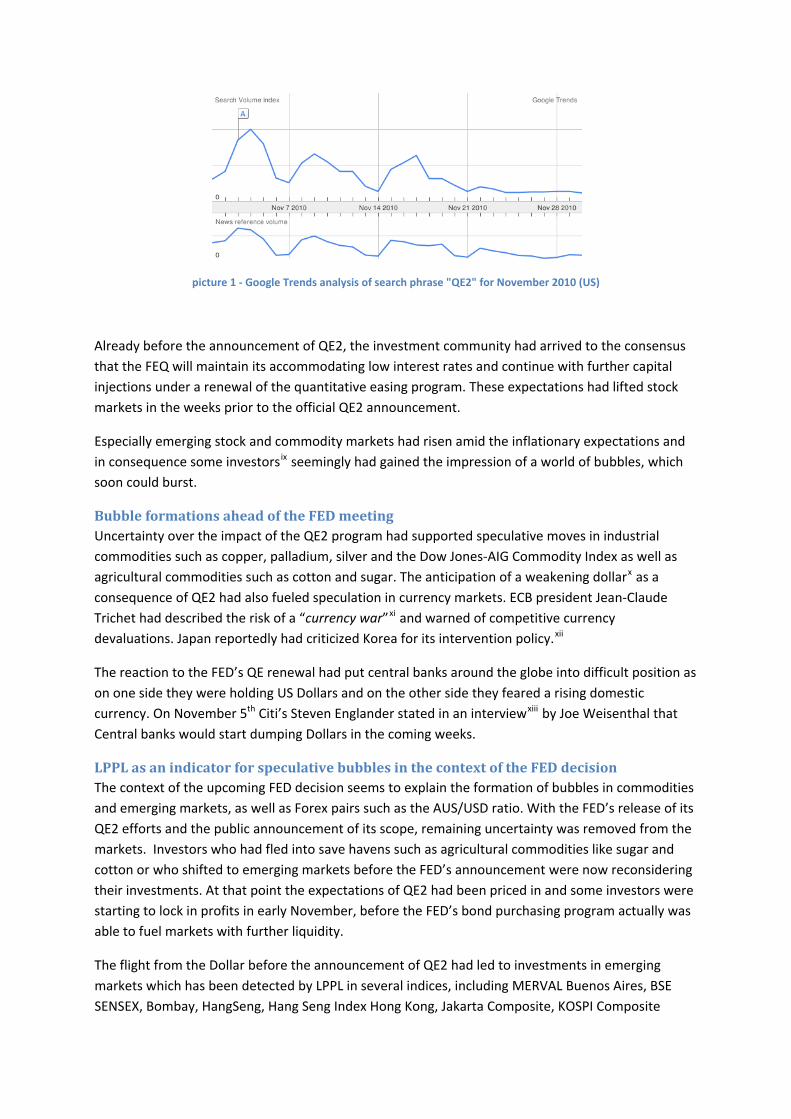
picture 1 ‐ Google Trends analysis of search phrase "QE2" for November 2010 (US)
Already before the announcement of QE2, the investment community had arrived to the consensus that the FEQ will maintain its accommodating low interest rates and continue with further capital injections under a renewal of the quantitative easing program. These expectations had lifted stock markets in the weeks prior to the official QE2 announcement.
Especially emerging stock and commodity markets had risen amid the inflationary expectations and in consequence some investorsix seemingly had gained the impression of a world of bubbles, which soon could burst.
Bubble formations ahead of the FED meeting Uncertainty over the impact of the QE2 program had supported speculative moves in industrial commodities such as copper, palladium, silver and the Dow Jones‐AIG Commodity Index as well as agricultural commodities such as cotton and sugar. The anticipation of a weakening dollarx as a consequence of QE2 had also fueled speculation in currency markets. ECB president Jean‐Claude Trichet had described the risk of a “currency war”xi and warned of competitive currency devaluations. Japan reportedly had criticized Korea for its intervention policy.xii
The reaction to the FED’s QE renewal had put central banks around the globe into difficult position as on one side they were holding US Dollars and on the other side they feared a rising domestic currency. On November 5th Citi’s Steven Englander stated in an interviewxiii by Joe Weisenthal that Central banks would start dumping Dollars in the coming weeks.
LPPL as an indicator for speculative bubbles in the context of the FED decision The context of the upcoming FED decision seems to explain the formation of bubbles in commodities and emerging markets, as well as Forex pairs such as the AUS/USD ratio. With the FED’s release of its QE2 efforts and the public announcement of its scope, remaining uncertainty was removed from the markets. Investors who had fled into save havens such as agricultural commodities like sugar and cotton or who shifted to emerging markets before the FED’s announcement were now reconsidering their investments. At that point the expectations of QE2 had been priced in and some investors were starting to lock in profits in early November, before the FED’s bond purchasing program actually was able to fuel markets with further liquidity.
The flight from the Dollar before the announcement of QE2 had led to investments in emerging markets which has been detected by LPPL in several indices, including MERVAL Buenos Aires, BSE SENSEX, Bombay, HangSeng, Hang Seng Index Hong Kong, Jakarta Composite, KOSPI Composite

Index, but also ETFs, such as EWS. Alternatively bubbles were detected in the FTSE and the NASDAQ indices, as well as several sub‐indices such as the NASDAQ Computer index.
Beside those, LPPL helped to detect further bubbles in “recession proof”xiv equity investments, such as the automotive replacement parts and accessories company AutoZone (AZO) as well as United Rentals (URI) a company with focus equipment rentals.
i Heritage Foundation, "2010 Index of Economic Freedom: Argentina," 2010. Available from Heritage Foundation website. Accessed on September 8, 2010. (HF 2010) ii John Detrixhe (13.10.2010) “HFreeport‐McMoRan Bonds Rise to Record After Moody’s Raises GradeH”, Bloomberg iii Patrick Hosking and David Robertson (27.11.2009) H“Dubai in deep water as ripples from debt crisis spread”H, The Times iv Ewing, Jack (27.04.2010). H"Cuts to Debt Rating Stir Anxiety in Europe"H, The New York Times v Peer Steinbrueck (19.01.2011) „Bankenkrise, Wirtschaftskrise, Eurokrise ‐ Peer Steinbrück zieht Bilanz Vortrag von Peer Steinbrück (Bundesfinanzminister a.D.)“, Phoenix vi Nassim Taleb, (12.11.2010), “Inside Track” Interview, HBloombergH vii Frank Berlage (1.11.2010) “THE REAL CRISIS”, source: Hhttp://new.gloomboomdoom.com viii Federalreserve (03.11.2010), HPress ReleaseH, Federalreserve ix Charles Wallace (09.11.2010) H“10 Market Bubbles, that could soon burst”H, www.DailyFinance.com x Jeff Cox (04.11.2010) „HDollar at Risk of Crashing, Triggering Inflation: StrategistH“, CNBC xi Marc Jones and Sakari Suoninen reporting on a news conference with Jean‐Claude Trichet (07.10.2010) „HECB warns of disruptive FX moves, holds policyH”, Reuters xii Bettina Schulz (19.10.2010) “HDie Fed forciert weitere Dollar‐AbwertungH“, FAZ xiii Joe Weisenthal (05.11.2010) „HCiti: Central Banks Are Going To Start Dumping Dollars In The Coming WeeksH”, thebusinessinsider.com xiv Jamie Dlugosch (04.03.2009) “HRecession‐Proof Stocks: AutoZone (AZO) Prospers as Automakers FalterH” Investorpalace.com

65
1 R. Woodard, D. Sornette, and M. Fedorovsky (The Financial Crisis Observatory), “The Finan-cial Bubble Experiment: advanced diagnostics and forecasts of bubble terminations, Vol. III–assetsdocument,” (2011), to be posted at http://www.er.ethz.ch/fco/ on 2 May 2011.
2 R. Woodard, D. Sornette, and M. Fedorovsky (The Financial Crisis Observatory), “The FinancialBubble Experiment: advanced diagnostics and forecasts of bubble terminations, Vol. III–masterdocument,” (2010).
3 Z.-Q. Jiang, W.-X. Zhou, D. Sornette, R. Woodard, K. Bastiaensen, and P. Cauwels, “doibase DOI: 10.1016/j.jebo.2010.02.007 Journal of Economic Behavior & Organization 74, 149 (2010).
4 A. Johansen, D. Sornette, and O. Ledoit, J. Risk 1, 5 (1999).5 A. Johansen and D. Sornette, Brussels Economic Review 53, 201.6 D. Sornette and A. Johansen, Quant. Financ. 1, 452 (2001).7 D. Sornette and W.-X. Zhou, Int. J. Forecast. 22, 153 (2006).8 D. Sornette, Why Stock Markets Crash: Critical Events in Complex Financial Systems (Princeton
University Press, Princeton, 2003).9 D. Sornette, R. Woodard, M. Fedorovsky, S. Reimann, H. Woodard, and W.-X. Zhou (The Finan-
cial Crisis Observatory), “The Financial Bubble Experiment: advanced diagnostics and forecasts ofbubble terminations,” (2009), http://arxiv.org/abs/0911.0454.
10 D. Sornette, R. Woodard, M. Fedorovsky, S. Reimann, H. Woodard, and W.-X. Zhou (The Finan-cial Crisis Observatory), “The Financial Bubble Experiment: advanced diagnostics and forecasts ofbubble terminations, Vol. II–master document,” (2010), http://arxiv.org/abs/1005.5675.

Item 3:Original Master documentidentifying the 27 assets,
created on 12 November 2010.The checksums (digital fingerprint)
of following documentappear in document of item 1
(reproduced here for convenience):
Document name
SHA256SUM 4994beab18293be021d751d513b6fec0776fde9cf74c0098f7da8657487d950d
SHA512SUM ee20582b696a2ce880870b513e7b9e7ebb67bfbe62e2cad50dd18276a5158765af6fdf88d9fef6e047526c40478a865c722cab041386aa8efdd95da24dd9239d
Standalone version of following document(to verify checksum)
available as
fbe 20110502 assets 3.pdf
at
http://www.er.ethz.ch/fco/index
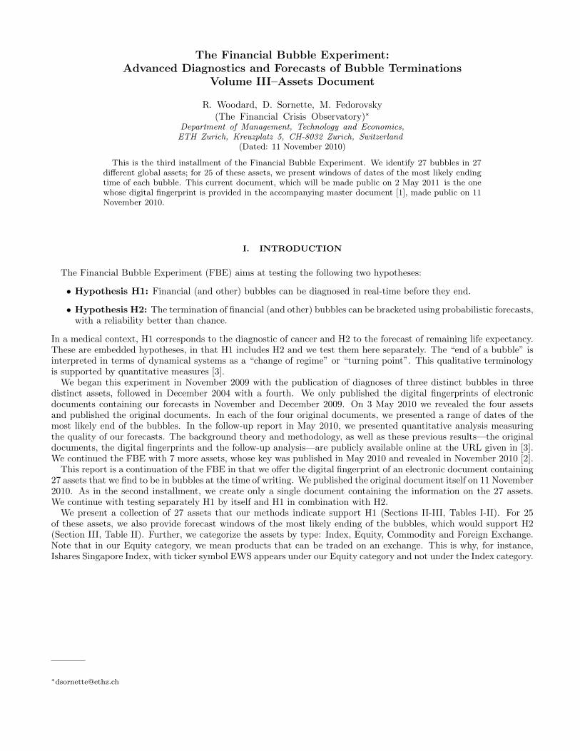
The Financial Bubble Experiment:Advanced Diagnostics and Forecasts of Bubble Terminations
Volume III–Assets Document
R. Woodard, D. Sornette, M. Fedorovsky
(The Financial Crisis Observatory)∗
Department of Management, Technology and Economics,ETH Zurich, Kreuzplatz 5, CH-8032 Zurich, Switzerland
(Dated: 11 November 2010)
This is the third installment of the Financial Bubble Experiment. We identify 27 bubbles in 27different global assets; for 25 of these assets, we present windows of dates of the most likely endingtime of each bubble. This current document, which will be made public on 2 May 2011 is the onewhose digital fingerprint is provided in the accompanying master document [1], made public on 11November 2010.
I. INTRODUCTION
The Financial Bubble Experiment (FBE) aims at testing the following two hypotheses:
• Hypothesis H1: Financial (and other) bubbles can be diagnosed in real-time before they end.
• Hypothesis H2: The termination of financial (and other) bubbles can be bracketed using probabilistic forecasts,with a reliability better than chance.
In a medical context, H1 corresponds to the diagnostic of cancer and H2 to the forecast of remaining life expectancy.These are embedded hypotheses, in that H1 includes H2 and we test them here separately. The “end of a bubble” isinterpreted in terms of dynamical systems as a “change of regime” or “turning point”. This qualitative terminologyis supported by quantitative measures [3].
We began this experiment in November 2009 with the publication of diagnoses of three distinct bubbles in threedistinct assets, followed in December 2004 with a fourth. We only published the digital fingerprints of electronicdocuments containing our forecasts in November and December 2009. On 3 May 2010 we revealed the four assetsand published the original documents. In each of the four original documents, we presented a range of dates of themost likely end of the bubbles. In the follow-up report in May 2010, we presented quantitative analysis measuringthe quality of our forecasts. The background theory and methodology, as well as these previous results—the originaldocuments, the digital fingerprints and the follow-up analysis—are publicly available online at the URL given in [3].We continued the FBE with 7 more assets, whose key was published in May 2010 and revealed in November 2010 [2].
This report is a continuation of the FBE in that we offer the digital fingerprint of an electronic document containing27 assets that we find to be in bubbles at the time of writing. We published the original document itself on 11 November2010. As in the second installment, we create only a single document containing the information on the 27 assets.We continue with testing separately H1 by itself and H1 in combination with H2.
We present a collection of 27 assets that our methods indicate support H1 (Sections II-III, Tables I-II). For 25of these assets, we also provide forecast windows of the most likely ending of the bubbles, which would support H2(Section III, Table II). Further, we categorize the assets by type: Index, Equity, Commodity and Foreign Exchange.Note that in our Equity category, we mean products that can be traded on an exchange. This is why, for instance,Ishares Singapore Index, with ticker symbol EWS appears under our Equity category and not under the Index category.
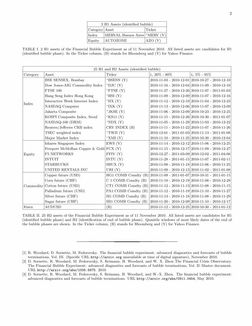
2
2 H1 Assets (identified bubble)
Category Asset Ticker
Index MERVAL Buenos Aires ^MERV (Y)
Equity AUTOZONE AZO (Y)
TABLE I. 2 H1 assets of the Financial Bubble Experiment as of 11 November 2010. All listed assets are candidates for H1(identified bubble phase). In the Ticker column, (B) stands for Bloomberg and (Y) for Yahoo Finance.
25 H1 and H2 Assets (identified bubble)
Category Asset Ticker tc 20% - 80% tc 5% - 95%
Index
BSE SENSEX, Bombay ^BSESN (Y) 2010-11-03 - 2010-12-01 2010-10-27 - 2010-12-10
Dow Jones-AIG Commodity Index ^DJC (Y) 2010-11-16 - 2010-12-04 2010-11-09 - 2010-12-10
FTSE 100 ^FTSE (Y) 2010-11-27 - 2010-12-26 2010-11-07 - 2011-01-03
Hang Seng Index Hong Kong ^HSI (Y) 2010-11-09 - 2010-12-09 2010-11-07 - 2010-12-16
Interactive Week Internet Index ^IIX (Y) 2010-11-12 - 2010-12-10 2010-11-04 - 2010-12-23
NASDAQ Computer ^IXK (Y) 2010-11-13 - 2010-12-06 2010-11-07 - 2010-12-09
Jakarta Composite ^JKSE (Y) 2010-11-06 - 2010-12-09 2010-10-23 - 2010-12-25
KOSPI Composite Index, Seoul ^KS11 (Y) 2010-11-15 - 2010-12-26 2010-10-30 - 2011-01-07
NASDAQ-100 (DRM) ^NDX (Y) 2010-11-05 - 2010-11-29 2010-11-03 - 2010-12-22
Reuters/Jefferies CRB index CRY INDEX (B) 2010-11-11 - 2010-11-22 2010-11-07 - 2010-11-26
TSEC weighted index ^TWII (Y) 2010-12-01 - 2011-01-03 2010-11-13 - 2011-01-08
Major Market Index ^XMI (Y) 2010-11-10 - 2010-11-25 2010-10-30 - 2010-12-04
Equity
Ishares Singapore Index EWS (Y) 2010-11-14 - 2010-12-12 2010-11-06 - 2010-12-25
Freeport McMoRan Copper & Gold FCX (Y) 2010-11-15 - 2010-12-17 2010-11-09 - 2010-12-27
F5 NETWORKS FFIV (Y) 2010-12-27 - 2011-03-09 2010-12-02 - 2011-04-08
INTUIT INTU (Y) 2010-11-28 - 2011-01-15 2010-11-07 - 2011-02-11
STARBUCKS SBUX (Y) 2010-11-08 - 2010-11-18 2010-11-06 - 2010-11-25
UNITED RENTALS INC URI (Y) 2010-11-09 - 2010-12-13 2010-11-02 - 2011-01-08
Commodity
Copper future (USD) HG1 COMB Comdty (B) 2010-11-09 - 2011-01-07 2010-10-31 - 2011-01-15
Corn future (CHF) C 1 COMB Comdty (B) 2010-11-18 - 2010-12-19 2010-11-08 - 2010-12-28
Cotton future (USD) CT1 COMB Comdty (B) 2010-11-12 - 2010-11-13 2010-11-08 - 2010-11-15
Palladium future (USD) PA1 COMB Comdty (B) 2010-11-12 - 2010-11-19 2010-11-10 - 2010-11-27
Silver future (CHF) SI1 COMB Comdty (B) 2010-11-13 - 2010-11-18 2010-11-08 - 2010-11-29
Sugar future (CHF) SB1 COMB Comdty (B) 2010-11-20 - 2010-12-09 2010-11-10 - 2010-12-17
Forex AUDUSD (B) 2010-11-12 - 2010-12-25 2010-10-30 - 2011-01-12
TABLE II. 25 H2 assets of the Financial Bubble Experiment as of 11 November 2010. All listed assets are candidates for H1(identified bubble phase) and H2 (identification of end of bubble phase). Quantile windows of most likely dates of the end ofthe bubble phases are shown. In the Ticker column, (B) stands for Bloomberg and (Y) for Yahoo Finance.
[1] R. Woodard, D. Sornette, M. Fedorovsky. The financial bubble experiment: advanced diagnostics and forecasts of bubbleterminations, Vol. III. (Specific URL http://arxiv.org unavailable at time of digital signature), November 2010.
[2] D. Sornette, R. Woodard, M. Fedorovsky, S. Reimann, H. Woodard, and W. X. Zhou The Financial Crisis Observatory.The Financial Bubble Experiment: advanced diagnostics and forecasts of bubble terminations, Vol. II–Master document.URL http://arxiv.org/abs/1005.5675. 2010.
[3] D. Sornette, R. Woodard, M. Fedorovsky, S. Reimann, H. Woodard, and W.-X. Zhou. The financial bubble experiment:advanced diagnostics and forecasts of bubble terminations. URL http://arxiv.org/abs/0911.0454, May 2010.

3
II. H1 ASSETS
We diagnose that the 2 assets in this Section (see Table I) are in a bubble phase (H1) but we do not make forecastsof likely dates of change of regime (H2). For each asset, we present a figure showing the time series of the observationsand indicate the range over which our analysis was performed (the shaded area in each figure).
A. H1 Indexes
1. MERVAL Buenos Aires
2008/02 2008/08 2009/02 2009/08 2010/02 2010/08date
800
1600
2400
3200
pric
e
last obs. price: 3311.0
last
obs
.: 20
10-1
1-10
MERV
Observed prices
FIG. 1. MERVAL Buenos Aires: Time series of observations (filled circles) and range over which our analysis was performed(shaded region).
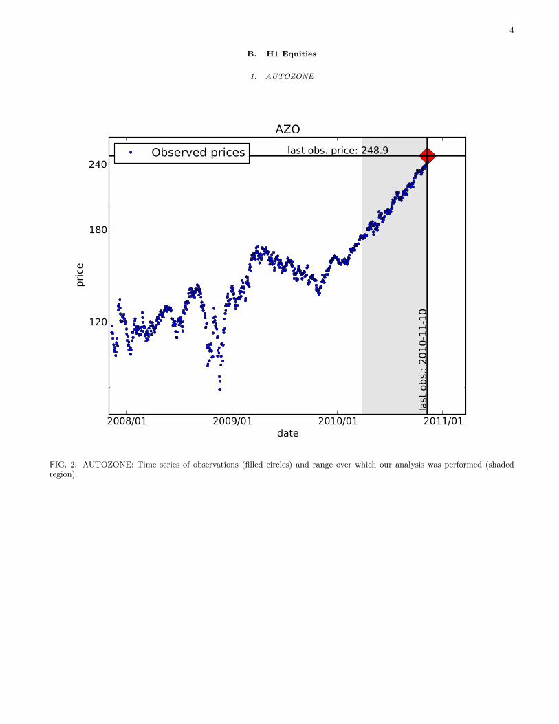
4
B. H1 Equities
1. AUTOZONE
2008/01 2009/01 2010/01 2011/01date
120
180
240
pric
e
last obs. price: 248.9
last
obs
.: 20
10-1
1-10
AZO
Observed prices
FIG. 2. AUTOZONE: Time series of observations (filled circles) and range over which our analysis was performed (shadedregion).

5
III. H1 & H2 ASSETS
We hypothesize that the 25 assets in this Section (see Table II) are all in a bubble phase (H1) and are likely to endwithin the quantile ranges indicated in Table II (H2).
A. H1 & H2 Indexes
1. BSE SENSEX, Bombay
2008/01 2009/01 2010/01 2011/01date
10000
15000
20000
25000
pric
e
last obs. price: 20875.7
last
obs
.: 20
10-1
1-10
20/80: 2010-11-03 - 2010-12-015/95: 2010-10-27 - 2010-12-1020/80: 2010-11-03 - 2010-12-015/95: 2010-10-27 - 2010-12-10
BSESN
Observed prices
FIG. 3. BSE SENSEX, Bombay: Time series of observations (filled circles) and range over which our analysis was performed(shaded region).

6
2. Dow Jones-AIG Commodity Index
2008/01 2009/01 2010/01 2011/01date
100
150
200
250
pric
e last obs. price: 154.2
last
obs
.: 20
10-1
1-10
20/80: 2010-11-16 - 2010-12-045/95: 2010-11-09 - 2010-12-1020/80: 2010-11-16 - 2010-12-045/95: 2010-11-09 - 2010-12-10
DJC
Observed prices
FIG. 4. Dow Jones-AIG Commodity Index: Time series of observations (filled circles) and range over which our analysis wasperformed (shaded region).
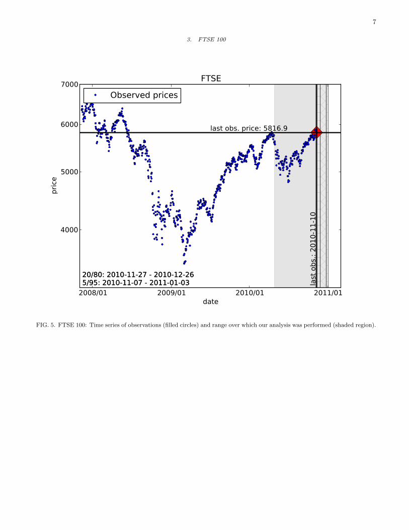
7
3. FTSE 100
2008/01 2009/01 2010/01 2011/01date
4000
5000
6000
7000
pric
e
last obs. price: 5816.9
last
obs
.: 20
10-1
1-10
20/80: 2010-11-27 - 2010-12-265/95: 2010-11-07 - 2011-01-0320/80: 2010-11-27 - 2010-12-265/95: 2010-11-07 - 2011-01-03
FTSE
Observed prices
FIG. 5. FTSE 100: Time series of observations (filled circles) and range over which our analysis was performed (shaded region).

8
4. Hang Seng Index Hong Kong
2008/01 2009/01 2010/01 2011/01date
16000
24000
32000
pric
e
last obs. price: 24500.6
last
obs
.: 20
10-1
1-10
20/80: 2010-11-09 - 2010-12-095/95: 2010-11-07 - 2010-12-1620/80: 2010-11-09 - 2010-12-095/95: 2010-11-07 - 2010-12-16
Hang Seng
Observed prices
FIG. 6. Hang Seng Index Hong Kong: Time series of observations (filled circles) and range over which our analysis wasperformed (shaded region).

9
5. Interactive Week Internet Index
2008/01 2009/01 2010/01 2011/01date
160
240
320
pric
e
last obs. price: 312.7
last
obs
.: 20
10-1
1-10
20/80: 2010-11-12 - 2010-12-105/95: 2010-11-04 - 2010-12-2320/80: 2010-11-12 - 2010-12-105/95: 2010-11-04 - 2010-12-23
IIX
Observed prices
FIG. 7. Interactive Week Internet Index: Time series of observations (filled circles) and range over which our analysis wasperformed (shaded region).
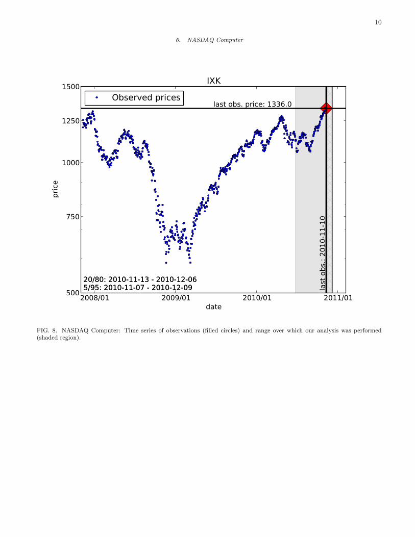
10
6. NASDAQ Computer
2008/01 2009/01 2010/01 2011/01date
500
750
1000
1250
1500
pric
e
last obs. price: 1336.0
last
obs
.: 20
10-1
1-10
20/80: 2010-11-13 - 2010-12-065/95: 2010-11-07 - 2010-12-0920/80: 2010-11-13 - 2010-12-065/95: 2010-11-07 - 2010-12-09
IXK
Observed prices
FIG. 8. NASDAQ Computer: Time series of observations (filled circles) and range over which our analysis was performed(shaded region).

11
7. Jakarta Composite
2008/01 2009/01 2010/01 2011/01date
1000
2000
3000
4000
pric
e
last obs. price: 3757.0
last
obs
.: 20
10-1
1-10
20/80: 2010-11-06 - 2010-12-095/95: 2010-10-23 - 2010-12-2520/80: 2010-11-06 - 2010-12-095/95: 2010-10-23 - 2010-12-25
JKSE
Observed prices
FIG. 9. Jakarta Composite: Time series of observations (filled circles) and range over which our analysis was performed (shadedregion).

12
8. KOSPI Composite Index, Seoul
2008/01 2009/01 2010/01 2011/01date
800
1200
1600
2000
pric
e
last obs. price: 1967.8
last
obs
.: 20
10-1
1-10
20/80: 2010-11-15 - 2010-12-265/95: 2010-10-30 - 2011-01-0720/80: 2010-11-15 - 2010-12-265/95: 2010-10-30 - 2011-01-07
KS11
Observed prices
FIG. 10. KOSPI Composite Index, Seoul: Time series of observations (filled circles) and range over which our analysis wasperformed (shaded region).

13
9. NASDAQ-100 (DRM)
2008/01 2009/01 2010/01 2011/01date
1000
1500
2000
2500
pric
e
last obs. price: 2187.7
last
obs
.: 20
10-1
1-10
20/80: 2010-11-05 - 2010-11-295/95: 2010-11-03 - 2010-12-2220/80: 2010-11-05 - 2010-11-295/95: 2010-11-03 - 2010-12-22
NDX
Observed prices
FIG. 11. NASDAQ-100 (DRM): Time series of observations (filled circles) and range over which our analysis was performed(shaded region).

14
10. Reuters/Jefferies CRB index
2008/02 2008/08 2009/02 2009/08 2010/02 2010/08date
200
300
400
500
pric
e
last obs. price: 317.1
last
obs
.: 20
10-1
1-10
20/80: 2010-11-11 - 2010-11-225/95: 2010-11-07 - 2010-11-2620/80: 2010-11-11 - 2010-11-225/95: 2010-11-07 - 2010-11-26
RJ CRB
Observed prices
FIG. 12. Reuters/Jefferies CRB index: Time series of observations (filled circles) and range over which our analysis wasperformed (shaded region).

15
11. TSEC weighted index
2008/01 2009/01 2010/01 2011/01date
4000
6000
8000
10000
pric
e
last obs. price: 8450.6
last
obs
.: 20
10-1
1-10
20/80: 2010-12-01 - 2011-01-035/95: 2010-11-13 - 2011-01-0820/80: 2010-12-01 - 2011-01-035/95: 2010-11-13 - 2011-01-08
TWII
Observed prices
FIG. 13. TSEC weighted index: Time series of observations (filled circles) and range over which our analysis was performed(shaded region).

16
12. Major Market Index
2008/01 2009/01 2010/01 2011/01date
750
1000
1250
1500
pric
e
last obs. price: 1245.2
last
obs
.: 20
10-1
1-10
20/80: 2010-11-10 - 2010-11-255/95: 2010-10-30 - 2010-12-0420/80: 2010-11-10 - 2010-11-255/95: 2010-10-30 - 2010-12-04
XMI
Observed prices
FIG. 14. Major Market Index: Time series of observations (filled circles) and range over which our analysis was performed(shaded region).

17
B. H1 & H2 Equities
1. Ishares Singapore Index
2008/01 2009/01 2010/01 2011/01date
8
12
16
pric
e
last obs. price: 14.4
last
obs
.: 20
10-1
1-10
20/80: 2010-11-14 - 2010-12-125/95: 2010-11-06 - 2010-12-2520/80: 2010-11-14 - 2010-12-125/95: 2010-11-06 - 2010-12-25
EWS
Observed prices
FIG. 15. Ishares Singapore Index: Time series of observations (filled circles) and range over which our analysis was performed(shaded region).

18
2. Freeport McMoRan Copper & Gold
2008/01 2009/01 2010/01 2011/01date
40
80
120
pric
e
last obs. price: 104.3
last
obs
.: 20
10-1
1-10
20/80: 2010-11-15 - 2010-12-175/95: 2010-11-09 - 2010-12-2720/80: 2010-11-15 - 2010-12-175/95: 2010-11-09 - 2010-12-27
FCX
Observed prices
FIG. 16. Freeport McMoRan Copper & Gold: Time series of observations (filled circles) and range over which our analysis wasperformed (shaded region).

19
3. F5 NETWORKS
2008/01 2009/01 2010/01 2011/01date
50
100
150
pric
e
last obs. price: 122.9
last
obs
.: 20
10-1
1-10
20/80: 2010-12-27 - 2011-03-095/95: 2010-12-02 - 2011-04-0820/80: 2010-12-27 - 2011-03-095/95: 2010-12-02 - 2011-04-08
FFIV
Observed prices
FIG. 17. F5 NETWORKS: Time series of observations (filled circles) and range over which our analysis was performed (shadedregion).

20
4. INTUIT
2008/05 2008/11 2009/05 2009/11 2010/05 2010/11date
20
30
40
50
pric
e
last obs. price: 48.8
last
obs
.: 20
10-1
1-10
20/80: 2010-11-28 - 2011-01-155/95: 2010-11-07 - 2011-02-1120/80: 2010-11-28 - 2011-01-155/95: 2010-11-07 - 2011-02-11
INTU
Observed prices
FIG. 18. INTUIT: Time series of observations (filled circles) and range over which our analysis was performed (shaded region).

21
5. STARBUCKS
2008/02 2008/08 2009/02 2009/08 2010/02 2010/08date
10
20
30
40
pric
e
last obs. price: 30.5
last
obs
.: 20
10-1
1-10
20/80: 2010-11-08 - 2010-11-185/95: 2010-11-06 - 2010-11-2520/80: 2010-11-08 - 2010-11-185/95: 2010-11-06 - 2010-11-25
SBUX
Observed prices
FIG. 19. STARBUCKS: Time series of observations (filled circles) and range over which our analysis was performed (shadedregion).

22
6. UNITED RENTALS INC
2008/01 2009/01 2010/01 2011/01date
10
20
30
pric
e
last obs. price: 20.2
last
obs
.: 20
10-1
1-09
20/80: 2010-11-10 - 2010-12-135/95: 2010-10-31 - 2011-01-0520/80: 2010-11-10 - 2010-12-135/95: 2010-10-31 - 2011-01-05
URI
Observed prices
FIG. 20. UNITED RENTALS INC: Time series of observations (filled circles) and range over which our analysis was performed(shaded region).
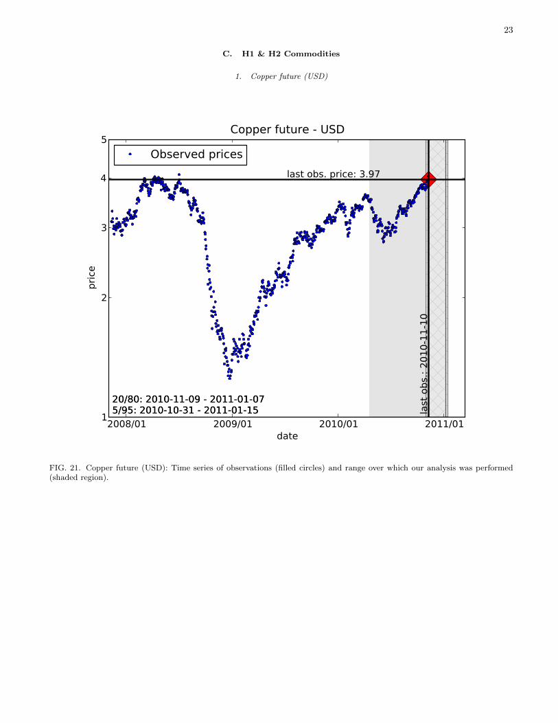
23
C. H1 & H2 Commodities
1. Copper future (USD)
2008/01 2009/01 2010/01 2011/01date
1
2
3
4
5
pric
e
last obs. price: 3.97
last
obs
.: 20
10-1
1-10
20/80: 2010-11-09 - 2011-01-075/95: 2010-10-31 - 2011-01-1520/80: 2010-11-09 - 2011-01-075/95: 2010-10-31 - 2011-01-15
Copper future - USD
Observed prices
FIG. 21. Copper future (USD): Time series of observations (filled circles) and range over which our analysis was performed(shaded region).
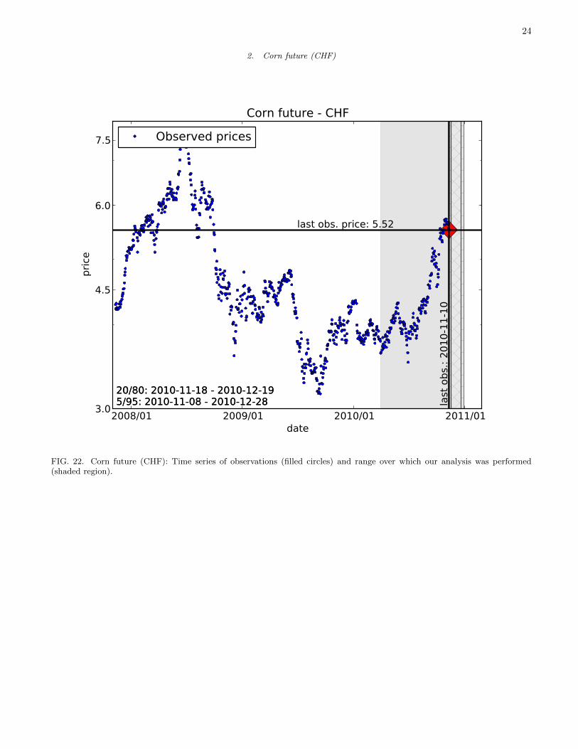
24
2. Corn future (CHF)
2008/01 2009/01 2010/01 2011/01date
3.0
4.5
6.0
7.5
pric
e
last obs. price: 5.52
last
obs
.: 20
10-1
1-10
20/80: 2010-11-18 - 2010-12-195/95: 2010-11-08 - 2010-12-2820/80: 2010-11-18 - 2010-12-195/95: 2010-11-08 - 2010-12-28
Corn future - CHF
Observed prices
FIG. 22. Corn future (CHF): Time series of observations (filled circles) and range over which our analysis was performed(shaded region).
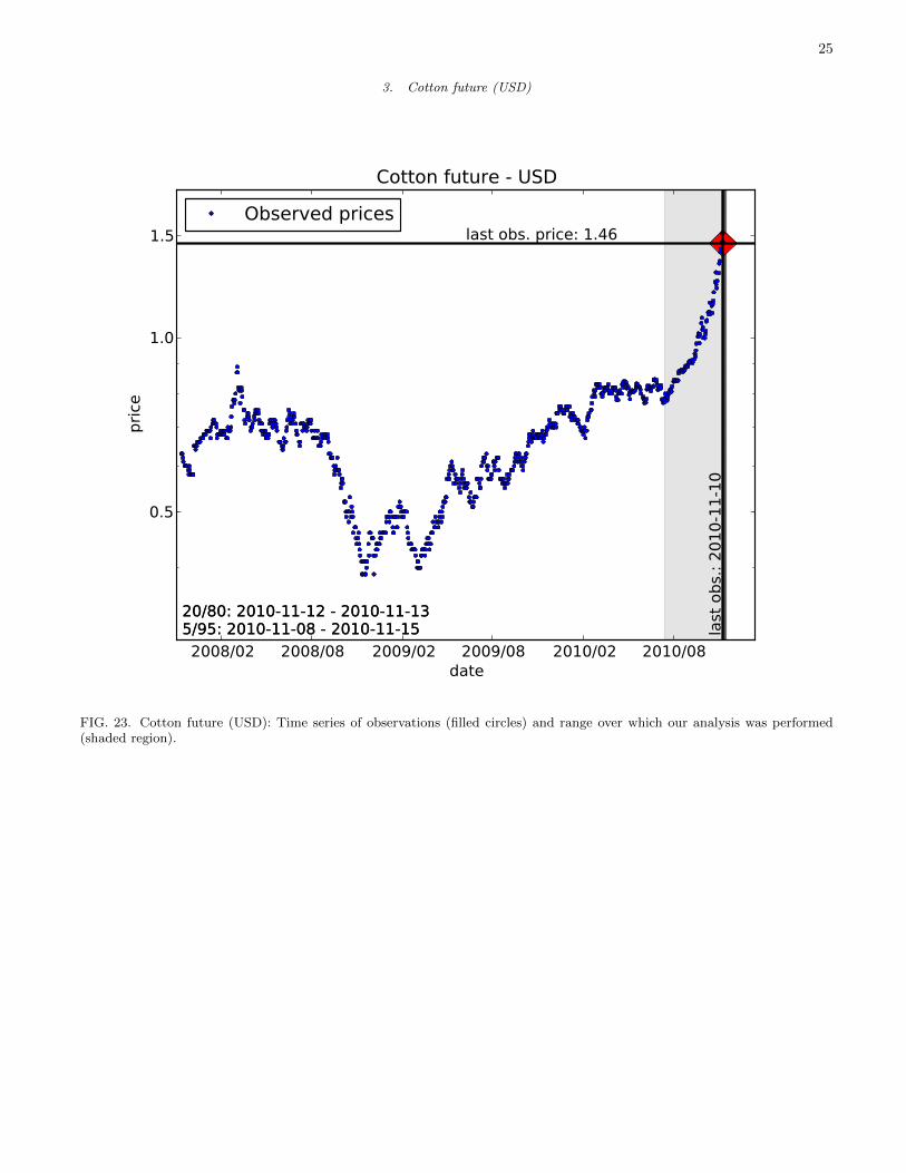
25
3. Cotton future (USD)
2008/02 2008/08 2009/02 2009/08 2010/02 2010/08date
0.5
1.0
1.5
pric
e
last obs. price: 1.46
last
obs
.: 20
10-1
1-10
20/80: 2010-11-12 - 2010-11-135/95: 2010-11-08 - 2010-11-1520/80: 2010-11-12 - 2010-11-135/95: 2010-11-08 - 2010-11-15
Cotton future - USD
Observed prices
FIG. 23. Cotton future (USD): Time series of observations (filled circles) and range over which our analysis was performed(shaded region).

26
4. Palladium future (USD)
2008/02 2008/08 2009/02 2009/08 2010/02 2010/08date
250
500
750
pric
e
last obs. price: 696.8
last
obs
.: 20
10-1
1-10
20/80: 2010-11-12 - 2010-11-195/95: 2010-11-10 - 2010-11-2720/80: 2010-11-12 - 2010-11-195/95: 2010-11-10 - 2010-11-27
Palladium future - USD
Observed prices
FIG. 24. Palladium future (USD): Time series of observations (filled circles) and range over which our analysis was performed(shaded region).

27
5. Silver future (CHF)
2008/02 2008/08 2009/02 2009/08 2010/02 2010/08date
16
24
32
pric
e
last obs. price: 26.2
last
obs
.: 20
10-1
1-10
20/80: 2010-11-13 - 2010-11-185/95: 2010-11-08 - 2010-11-2920/80: 2010-11-13 - 2010-11-185/95: 2010-11-08 - 2010-11-29
Silver future - CHF
Observed prices
FIG. 25. Silver future (CHF): Time series of observations (filled circles) and range over which our analysis was performed(shaded region).
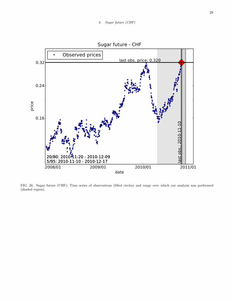
28
6. Sugar future (CHF)
2008/01 2009/01 2010/01 2011/01date
0.16
0.24
0.32
pric
e
last obs. price: 0.320
last
obs
.: 20
10-1
1-10
20/80: 2010-11-20 - 2010-12-095/95: 2010-11-10 - 2010-12-1720/80: 2010-11-20 - 2010-12-095/95: 2010-11-10 - 2010-12-17
Sugar future - CHF
Observed prices
FIG. 26. Sugar future (CHF): Time series of observations (filled circles) and range over which our analysis was performed(shaded region).

29
D. H1 & H2 Foreign Exchange
1. AUDUSD
2008/01 2009/01 2010/01 2011/01date
0.6
0.8
1.0
pric
e
last obs. price: 1.00
last
obs
.: 20
10-1
1-10
20/80: 2010-11-12 - 2010-12-255/95: 2010-10-30 - 2011-01-1220/80: 2010-11-12 - 2010-12-255/95: 2010-10-30 - 2011-01-12
AUDUSD
Observed prices
FIG. 27. AUDUSD: Time series of observations (filled circles) and range over which our analysis was performed (shaded region).