(The Final) CountdownPreprint

Jean-Marc Alliot∗

AbstractThe Countdown game is one of the oldest TV show run-ning in the world. It started broadcasting in 1972 on thefrench television and in 1982 on British channel 4, andit has been running since in both countries. The game,while extremely popular, never received any serious sci-entific attention, probably because it seems too simpleat first sight. We present in this article an in-depth anal-ysis of the numbers round of the countdown game. Thisincludes a complexity analysis of the game, an analysisof existing algorithms, the presentation of a new algo-rithm that increases resolution speed by a factor of 20.It also includes some leads on how to turn the game intoa more difficult one, both for a human player and for acomputer, and even to transform it into a probably un-decidable problem.

1 IntroductionThe Countdown (Wikipedia [2015]) game is one of theoldest TV show running in the world. It started broad-casting in 1972 on the french television as “des chiffreset des lettres”, literally “numbers and letters” with anumbers round called “Le compte est bon”, literally“the count is good”). It started broadcasting in 1982on British channel 4 as “Countdown”, and it has beenrunning since in both countries.

The numbers round of the game is extremely simple:6 numbers are drawn from a set of 24 which containsall numbers from 1 to 10 (small numbers) twice plus25, 50, 75 and 100 (large numbers). Then, with thesesix numbers, the contestants have to find a number ran-domly drawn between 101 and 9991, or, if it is impos-sible, the closest number to the number drawn. Onlythe four standard operations (+ − × /) can be used.

∗Institut de Recherche en Informatique de Toulouse1Whether 100 is a possible number to search is a matter of con-

troversy. It seems like it could be in the UK, but not in France, so wedecided to let it out.

As soon as two numbers have been used to make a newone, they can’t be used again, but the new number foundcan be used. For example, if the six numbers drawn are1,1,4,5,6,7 and the number to find is 899 the answer is:

Operations Remaining6 x 5 = 30 {1,1,4,7,30}

30 + 1 = 31 {1,4,7,31}4 x 7 = 28 {1,28,31}

28 + 1 = 29 {29,31}29 * 31 = 899 {899}

There are usually different ways to find a solution.The simplest answer is usually defined as the answerusing the least number of operations, and if two solu-tions have the same number of operations, a possiblerefinement is to keep the one having the smallest high-est number2.

The game, while extremely popular, never receivedany serious scientific attention. There was a very earlyarticle in the french magazine “l’Ordinateur Individuel”in the late seventies, written by Jean-Christophe Buis-son (Buisson [1980]), which described a simple algo-rithm. The only article written on the subject in En-glish was published twice (Defays [1990, 1995a]) byDaniel Defays. Defays also published in 1995 a book infrench (Defays [1995b]) which used the game as a cen-tral example for introducing artificial intelligence meth-ods. But the ultimate goal of Defays was not to de-velop an accurate solver for the game, but a solver mim-icking human reasoning (such as the Jumbo programby Hofstadter), including possible mistakes (in French,Defays sometimes named his program “le compte estmauvais”, literally the count is bad, a joke on the orig-inal name of the game, indicating that it might makemistakes while searching for the solution).

There are many commercial or free programs devel-oped for this game. Some of them are bugged or use

2There are a few differences between the french and the Britishgame. In the french version, all numbers are drawn at random while inthe British game, the contestants can choose how many large numberswill be present in the six numbers set.

1

arX

iv:1

502.

0545

0v1

[cs

.AI]

19

Feb

2015

incomplete or incorrect algorithms. Many websites inFrance and in Great Britain discuss the game and how toprogram it, with lot of code, lot of statistics, and some-times lot of errors. The first goal of this article is to doa scientific analysis of the game regarding its complex-ity and to provide a set of cutting edge algorithms andcodes to solve it properly. Its second goal is to inves-tigate potential extension of the games, either to turn itinto a more complex problem, or into a (maybe) unde-cidable problem on some of its instances.

We use a few mathematical symbols and functions inthis paper: n! is the factorial of n, Cp

n = n!p! (n−p)! is

the number of subsets having p elements in a set of ndistinct elements, Γ(z) is the Euler Gamma function,E(x) is the integer part of x.

2 Elementary algorithms

2.1 Decomposition in sub-problems

The first published algorithm (Buisson [1980]) used asimple decomposition mechanism. Let’s consider thefollowing example: numbers 3, 50, 7, 4, 75, 8, numberto find 822. The algorithm would start from the solution(822) and use a backward chaining approach in the Pro-log way. However, not all operations were tried; at oddsteps, only addition and subtractions were used, whileat even steps only divisions were used. So the algorithmwould at the first step generate thirteen numbers: 822,822 ± 3, 822 ± 50, . . . , and then try to divide all ofthem by the remaining 5 (or 6 if no number was addedor subtracted) numbers. If a division succeeds, the al-gorithm would then be applied recursively on the newresult with the remaining numbers. Here the solutioncan be found by:

Operations Remaining(822 + 50) / 4 = 218 {3,7,75,8}(218 + 7) / 3 = 75 {75,8}75 - 75 = 0 {8}

When 0 is reached the solution has been found.The complexity of this algorithm is very low. If we

have n numbers, we first generate 2n + 1 numbers andtry to divide them by n − 1 numbers, so we have to do(2n + 1)(n − 1) trial divisions. At the next step, wewould have on the average 2(n − 2) + 1 numbers todivide by n− 3 numbers, so (2(n− 2) + 1)(n− 3) trialdivisions, and so on.

On the one hand, if all divisions succeed, we have a

maximal complexity of:

n/2∏i=1

(4i+ 1)(2i− 1) =2

3n2 Γ(n2 + 5

4

)Γ(n+12

)√πΓ(54

)' 8

n2 ((

n

2)!)2

On the other hand, if only one division succeedsat each step, the minimal complexity is:

∑n/2i=1(4i +

1)(2i − 1) = n3+9n−412 For n = 6, we have a maxi-

mal complexity of 8775 trial divisions, and a minimalcomplexity of 97 trial divisions.

This algorithm was popular in the seventies, whenmachines were slow, with only 8 bit addition and sub-traction in hardware, with division and multiplicationimplanted in software on microprocessors. Moreover,programs were often written using slow, interpreted lan-guages. Some of the initial programs were written inBasic or in Prolog, and could not handle a large num-ber of computations in the 30 or 45s allowed by thegame. Indeed, this algorithm was published again in1984 (Froissart [1984]) in another journal, which meansthat even 4 years later, few people were able to writeprograms to solve completely the game.

This algorithm has of course serious drawbacks. It isimpossible to compute solutions requiring intermediateresults, such as the first one presented in this article,because 31 and 29 must be built independently beforemultiplying them to have 899. It is even impossible tofind solutions with divisions. Moreover, this methodcan only find the exact result. If it doesn’t exist, thecomputation has to be restarted with the closest numberto the number to find as a new goal.

This algorithm was later refined with faster machinesby using all possible operations at each step. At the firststep of the algorithm there are 6 numbers available and4 possible operations, which would give 24 numbers atmost (here: 822 + 3, 822− 3, 822× 3, 822/3 and so onwith 50, 7, 4. . . ). Division is not always possible, and sothere are in fact between 18 and 24 numbers (here thereare only 19 numbers at the first step, as 822 can onlybe divided by 3). This algorithm is recursively applieduntil 0 is found or until no number remains in the poolof available numbers.

Here, the solution can be found in the following way:

822 + 50 = 872 {3,7,4,75,8}872 / 4 = 218 {3,7,75,8}218 + 7 = 225 {3,75,8}225 / 3 = 75 {75,8}75 - 75 = 0 {8}

2

The maximal complexity of the algorithm is (6×4)×(5 × 4) × · · · (1 × 4) = 6! 46 If we consider the gen-eral case with n numbers the complexity is n! 4n. Forn = 6, the maximal number of operations is 491520.If we consider that the actual number of operations ateach step is closer to 3 than to 4, we have a minimalcomplexity of n! 3n, and for n = 6 the minimal num-ber of operations is 87480. Let’s also keep in mind thateven if division is not possible it has to be tested be-fore being discarded, so this minimal complexity is aninferior bound that can never be reached.

This refinement adds more solutions but it is still im-possible to find solutions requiring intermediate results,and impossible to find directly approximate results.

2.2 The depth first algorithmThe recursive depth first algorithm is extremely easy tounderstand. Let’s consider the complete set of n num-bers. We simply pick two of them (C2

n = n(n−1)2 possi-

bilities) and combine them using one of the four possi-ble operations. The order of the two numbers picked isirrelevant as the order does not matter for the additionand the multiplication (a+b = b+a and a×b = b×a),and we can only use one order for the other two opera-tions (if a > b, we can only compute a− b and a/b, andif a < b, b − a and b/a). Then we put back the resultof the computation in the set, giving a new set of n− 1numbers. We just repeat the algorithm until no numberremain in the pool and then backtrack to the previouspoint of choice, be it a number or an operation. This isa simple depth-first search algorithm, which is exhaus-tive as it searches the whole computation tree.

The maximal complexity of the algorithm is givenby: (n×(n−1)

2 ×4)×( (n−1)×(n−2)2 ×4)×· · ·×( 2×1

2 ×4).This gives:

dmax(n) = n! (n− 1)! 2n−1 (1)

dmin(n) = n! (n− 1)! (3

2)n−1 (2)

For n = 6, we have a maximal number of 2764800operations and a minimal number of 656100 operations.The algorithm is extremely easy to implement in thisnaive version. No complex data structures are needed,and being a depth first algorithm, it requires almost nomemory.

The first recorded implementation of this algo-rithm (Alliot [1986]) was developed for an Amiga 1000(a MC68000 based microcomputer with a 7MHz clock).

It was written in assembly language and solved thegame in less than 30s. However, this implementationwas not perfect, as it worked only with unsigned shortintegers (integers between 0 and 65535), and was thusunable to compute numbers that required intermediateresults higher than 65535 (and there are some, such asfinding 996 with {3, 3, 25, 50, 75, 100} which requiresusing 99600 as an intermediate result).

2.3 The breadth first algorithmThe breadth first algorithm is a little bit more difficultto understand. It is also a recursive algorithm, but itworks on the partitions of the set of numbers. The firstpresentation of this algorithm seems to be Pin [1998].

• First, we create all sets generated by only one ele-ment. With the same example, we have of course6 elements g({3}) = {3}, g({50}) = {50},g({7}) = {7}, g({4}) = {4}, g({75}) = {75},g({8}) = {8}

• Next we create the sets of all numbers that canbe computed using only two numbers. Here forexample all the numbers generated by {3, 50}are the elements of g({3}) applied to the ele-ments of g({50}) which give the set g({3, 50}) =g({3}).g({50}) = {53, 47, 150}. {3} and {7}give g({3, 7}) = {10, 4, 21}. {50} and {7} giveg({50, 7}) = {57, 43, 350}. We will haveC2

6 suchsets.

• Next we create the sets of all numbers that can becomputed using only 3 numbers. For example,the set of numbers generated by the 3 numbers 3,50 and 7 is g({3, 50, 7}) = g({3}).g({50, 7}) ∪g({50}).g({3, 7}) ∪ g({7}).g({50, 3})Here for example g({3}).g({50, 7}) ={54, 60, 171, 19, 40, 46, 129, 347, 353, 1050}There are C3

6 such sets.

• The algorithm proceeds with all sets gen-erated by 4 numbers. For example the setgenerated by {3}, {50}, {7} and {4} isg({3, 50, 7, 4}) = g({3}).g({50, 7, 4}) ∪g({50}).g({3, 7, 4}) ∪ g({7}).g({50, 3, 4}) ∪g({4}).g({3, 50, 7}) ∪ g({3, 50}).g({7, 4}) ∪g({3, 7}).g({50, 4})∪ g({3, 4}).g({50, 7}) Thereare C4

6 such sets.

• We proceed with all sets generated by 5 numbers,applying exactly the same algorithms. There are

3

C56 such sets.

• Then we create the set generated by all six num-bers.

The complexity of this algorithm is not so easy tocompute. It is sometimes mistakenly presented as being2n (Mochel [2003]), but it is a very crude estimation.

If we callN(p) the number3 of elements in a set gen-erated by p elements, the total number of operations willbe∑n

p=1 CpnN(p). We still have to computeN(p). It is

possible to establish a recurrence relationship betweenN(p) and N(p− 1), N(p− 2), etc. Let’s see that on anexample. N(4) is the sum of two terms:

• N(3)×N(1)× 4×C34 which is the number of el-

ements in a set built by combining with the 4 oper-ations a set havingN(1) elements and a set havingN(3) elements. There are C3

4 = 4 such numbers.For example for {1, 2, 3, 4}, we have {1, 2, 3}.{4},{1, 2, 4}.{3}, {1, 3, 4}.{2}, {2, 3, 4}.{1}

• N(2) × N(2) × 4 × (C24/2) For exam-

ple, for {1, 2, 3, 4} we combine {1, 2}.{3, 4},{1, 3}.{2, 4} and {1, 4}.{2, 3}

More generally, we have:N(p) = (

∑p−1i=1 C

ipN(i)N(p− i))/2× 4

A simple computation gives:N(p) = 4p−1

∏p−1i=1 (2i− 1)

And thus the complexity for n numbers is:

bmax(n) =

n∑p=1

Cpn 4p−1

p−1∏i=1

(2i− 1) (3)

bmin(n) =

n∑p=1

Cpn 3p−1

p−1∏i=1

(2i− 1) (4)

For n = 6 we have a maximal number of 1144386 oper-ations, half the number of the operations required by thedepth first algorithm, and a minimal number of 287331operations.

3 Implementation and refinementsTo compare the algorithms, the programs were all writ-ten in Ocaml (INRIA [2004]). The implementation wasnot parallel and the programs were run on a 980X. For

3The N(p) are probably related to Bell numbers, but they are notthe same

very large instances, an implementation of the best al-gorithm (depth first with hash tables) was written in Cand assembly language. MPI (board [1997]) was usedto solve problems in parallel and the program was usedon a 640 AMD-HE6262 cores cluster using 512 cores.With the same algorithm, the C program on a singlecore is twice faster than the Ocaml program.

The 980X used in this section is a 6 cores Intel pro-cessor running at 3.33Ghz (a clock cycle of 0.3ns) witha 32kb+32kb L1 cache by core, a 256kb L2 cacheby core and 12Mb of L3 (Last Level Cache or LLC)cache common to all cores. Memory timings (Levinthal[2009]) for the Core i7 family and Xeon 5500 family areroughly of 4 clock cycles for L1 cache and 10 cycles forL2 cache. L3 cache access times depend on whether thedata is local to the core (40 cycles), shared with anothercore (65 cycles) or modified by another core (75 cy-cles). Here, the application is completely local to onecore, so it is safe to assume an access time of 40 cycles.Outside the L3 cache, access times depend on the num-ber and type of DIMMs, frequency of the memory bus,etc. . . A good guess is around 60ns, which is around 5times slower than the L3 cache (40 cycles takes approx-imately 12ns).

In this section we study the standard countdowngame: n = 6 numbers are drawn from a pool of 24,with all numbers in the range 1-10 present twice, plusone 25, one 50, one 75 and one 100. The number ofdifferent possible instances is:

C614 with no pair

+ C110 × C4

13 with one pair+ C2

10 × C212 with two pairs

+ C310 with three pairs

= 13243

Programs are so fast that trying to accurately measurethe execution time of a single instance is impossible.So, in the rest of this section, all programs solve thecomplete set of instances and the time recorded is thetime to complete the entire set: when a time of 160sis given, the mean time of resolution of one instance is160/13243 = 0.01s

3.1 The depth first algorithmImplementing the naive version of the depth-first algo-rithm is a straightforward process. First the algorithm

4

searches the entire space with the pool of initial num-bers and marks all numbers reached as being solvable.Then if the number to find is marked, it is solvable. Incase of failure, there is no need to start a new search:finding the closest number marked as solvable in the ar-ray is enough.

Storing solutions is easy: each time we compute anumber, we first check if it has been found already. If ithasn’t been found, we store the list of operations whichled to it (the list to store is just the branch currentlysearched). If the number has already been found, westore the new solution if and only if the list of operationsfor this solution is smaller than the one already stored.The algorithm being a depth first algorithm, we have noguarantee that the first solution found is the shortest.

There are a few simple improvements to implement,that will be used by all subsequent programs:

• never divide by 1, because it doesn’t generate anynew number.

• never multiply by 1 for the same reason.

• never subtract two equal numbers

• if a− b returns b then discard this branch

• if a/b returns b discard also this branch

• as stated in the previous section, it is useless to testthe pair (a, b) and the pair (b, a). If a >= bwe justcompute a + b, a ∗ b, a − b and a/b (if b dividesa). If b > a, we use b− a instead of a− b and b/ainstead of a/b.

The performance of the algorithm is good: the nativecode version solves the complete problem (the 13243instances) in 160s, or a mean of 0.01s by instance.

3.2 The depth first algorithm with hashtables

The idea is to use for this problem an (old) (Zobrist[1970]) improvement which has been often used inmany classical board games: hash tables.

First, we notice that, when solving the game, if thesame set of numbers appears a second time in the res-olution tree, the branch can be discarded: as it is adepth first search where the size of the set of numbersstrictly decreases by one at each level in the tree, weknow that this branch has already been fully developedsomewhere else in the tree and that all possible results

have already been computed and all numbers that canbe found with that set of numbers have already beenmarked. We just need a way to uniquely identify anidentical set of numbers, and to do this in a very shortamount of time as this test will take place each time anew number is generated.

There is, as usual with hash tables, a trade-off be-tween generality (being able to identify any set andstore all hash values) and speed (losing some general-ity to be faster). There are two main problems whenusing hash tables: computing the hash value and stor-ing/retrieving it.

For computing the hash value, Ocaml provides ageneric hash function that operates on any object andreturns a positive integer that can be used as an identi-fier of the object. However, using this function on setsof numbers proved to be much too slow. Thus a faster,incremental approach, was used: an array h(x) of 64bits random values is created at the start of the program.Each time a number x is added to the pool of numbers,h(x) is added to the hash value, and when x is removedfrom the pool, h(x) is subtracted from the hash value.This is slightly different from the hash computation inboard games where the function used is the faster xorfunction, both for adding and removing objects. How-ever, xor can not be used here as two identical numberscan be in the pool at the same time and would cancel outeach other: the set {1, 1, 2, 3, 4} would have the samehash value as {2, 3, 4}.

Storing the hash value required some experimentaltests. Using a single set structure to store all values wasruled out from the start, as it would have been way tooslow (the log n access time is too important). Thus amore classical array structure was chosen, where a maskof n-bits was applied to the 64-bits hash value, returningan index for this array (the size of the array is of course2n). There were two remaining problems to solve: howto handle hash collisions and how large the array mustbe.

Hash collisions happen when two different objectshaving different hash values have the same hash index.They can be solved in two (main) ways: maintaining aset of values for each array element, or having a largerarray to minimize hash collisions. However having atoo large array can also have detrimental consequences:as the access to the hash array is mostly random, cachefaults are very likely to happen at each access if the ar-ray doesn’t fit in the cache. The largest the part of thearray out of the cache, the higher the probability to havea cache fault and to seriously slow down the program.

5

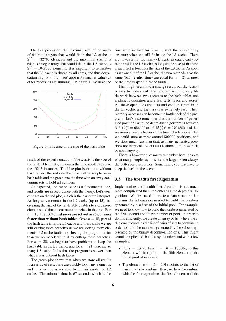
On this processor, the maximal size of an arrayof 64 bits integers that would fit in the L2 cache is215 = 32768 elements and the maximum size of a64 bits integer array that would fit in the L3 cache is220 = 1048576 elements. It is important to rememberthat the L3 cache is shared by all cores, and thus degra-dation might (or might not) appear for smaller values asother processes are running. On figure 1, we have the

0

50

100

150

200

250

8 10 12 14 16 18 20 22

hashhash_setno_accel

Figure 1: Influence of the size of the hash table

result of the experimentation. The x-axis is the size ofthe hash table in bits, the y-axis the time needed to solvethe 13243 instances. The blue plot is the time withouthash tables, the red one the time with a simple arrayhash table and the green one the time with an array con-taining sets to hold all numbers.

As expected, the cache issue is a fundamental one,and results are in accordance with the theory. Let’s con-centrate on the red plot, which is the easiest to interpret.As long as we remain in the L2 cache (up to 15), in-creasing the size of the hash table enables to store moreelements and thus to cut more branches in the tree. Forn = 15, the 13243 instances are solved in 26s, 5 timesfaster than without hash tables. Over n = 15, part ofthe hash table is in the L3 cache and thus, while we arestill cutting more branches as we are storing more ele-ments, L2 cache faults are slowing the program fasterthan we are accelerating it by cutting more branches.For n = 20, we begin to have problems to keep thehash table in the L3 cache, and for n = 21 there are somany L3 cache faults that the program is slower thanwhat it was without hash tables.

The green plot shows that when we store all resultsin an array of sets, there are quickly too many elements,and thus we are never able to remain inside the L2cache. The minimal time is 67 seconds which is the

time we also have for n = 19 with the simple arraystructure when we still fit inside the L3 cache. Thereare however not too many elements as data clearly re-main inside the L3 cache as long as the size of the hasharray itself is less than the size of the L3 cache. As soonas we are out of the L3 cache, the two methods give thesame (bad) results: times are equal for n = 21 as mostof the time is spent in cache faults.

This might seem like a strange result but the reasonis easy to understand: the program is doing very lit-tle work between two accesses to the hash table: onearithmetic operation and a few tests, reads and stores.All these operations use data and code that remain inthe L1 cache, and they are thus extremely fast. Then,memory accesses can become the bottleneck of the pro-gram. Let’s also remember that the number of gener-ated positions with the depth-first algorithm is between6! 5! ( 3

2 )5 = 656100 and 6! 5! ( 42 )5 = 2764800, and that

we never store the leaves of the tree, which implies thatwe could store at most around 500000 positions, andwe store much less than that, as many generated posi-tions are identical. As 500000 is almost 219, n = 21 isoverkill anyway.

There is however a lesson to remember here: despitewhat many people say or write, the larger is not alwaysthe better for hash tables. Sometimes, you first have tokeep the hash in the cache.

3.3 The breadth first algorithmImplementing the breadth first algorithm is not muchmore complicated than implementing the depth first al-gorithm. We first need to create a data structure thatcontains the information needed to build the numbersgenerated by a subset of the initial pool. For example,we need to know how to build the numbers generated bythe first, second and fourth number of pool. In order todo this efficiently, we create an array of list where the i-th element contains the list of pairs of sets to combine inorder to build the numbers generated by the subset rep-resented by the binary decomposition of i. This mightsound complicated, but is easy to understand with a fewexamples:

• For i = 16 we have i = 16 = 100002, so thiselement will just point to the fifth element in theinitial pool of numbers.

• The element at i = 5 = 1012 points to the list ofpairs of sets to combine. Here, we have to combinewith the four operations the first element and the

6

third element of the original pool, so there is onlyone pair (1, 3).

• The element at i = 25 = 110012 will contain thepairs (1, 24), (8, 17) and (9, 16) because to haveall elements generated by the first, the fourth andthe fifth element of the original pool we have tocombine with the four operations (a) all elementsgenerated by the fourth and the fifth with the firstelement, (b) all elements generated by the first andthe fourth with the fifth element and (c) all ele-ments generated by the first and the firth with thefourth element.

• The element at i = 57 = 1110012 will contain:

– the pairs (1, 56), (8, 49), (16, 41) and(32, 25) which are the numbers generated bythe subsets generated by three elements tocombine with the numbers generated by thesubsets of one element

– the pairs (9, 48), (17, 40), (33, 24) which arethe numbers generated by the subsets gen-erated by two elements combined with theother numbers generated by the subsets of thecomplementary two elements subsets.

This array of list of pairs can be pre-computed andstored once and for all. The size of the array is 2n − 1where n = 6, so the array here has 63 lists of pairs.

The rest of the algorithm is straightforward. Anotherarray of the same size is used, where the i-th element isan array that will hold all numbers generated for the iindex.

Let’s see that on an example. If the initial pool ofnumbers is {7, 8, 9, 10, 25, 75} we first copy 7 at posi-tion 1, 8 at position 2, 9 at position 4, 10 at position 8, 25at position 16 and 75 at position 32. Then, all elementswith an index having only 1 bit are filled. Then we fillall elements having an index with 2 bits. For example,element 3 = 112 is {7 + 8, 8− 7, 7× 8} = {15, 1, 56},element 5 = 1012 is {7+9, 9−7, 9×7} = {16, 2, 63},element 6 = 1102 is {17, 1, 72}, and so on. Whenall elements with a 2-bits index are filled, elementswith a 3-bits index are filled. For example element7 = 1112 is {15 + 9, 15− 9, 15× 9, 1 + 9, 9− 1, 56 +9, 56− 9, 56× 9} ∪ {16 + 8, 16− 8, 16 ∗ 8, 16/8, 2 +8, 8 − 2, 8 × 2, 8/2, 63 + 8, 63 − 8, 63 × 8} ∪ {17 +7, 17 − 7, 17 × 7, 1 + 7, 7 − 1, 72 + 7, 72 − 7, 72 ×7} = {24, 6, 135, 10, 8, 65, 47, 504, 24, 8, 128, 2, 10, 6,16, 4, 71, 55, 504, 24, 10, 119, 8, 6, 79, 65, 504}.

There remains a few implementation details to solve.Whether it is better to use an array of arrays or an arrayof sets is unclear. Both structures have their advantagesand their disadvantages. An array has an access timewhich is constant, while inserting a new number in aset of size n takes log n operations when using a binarybalanced tree structure for the set. However, when us-ing sets, duplicates numbers are never kept and thereare lot of duplicates: even in the simple example above,there are already many of them in the 3-bits 7th element.Another (minor) advantage of the sets is that they useexactly the right number of elements while the size ofarrays has to be pre-computed at allocation time; how-ever this minor point may be circumvented in differentways: first we know a quite good estimate of the sizeof each array, as the N(p) numbers computed in sec-tion 2.3 are an upper bound of the size of a p-bits array.Moreover, it is possible to break the (large) arrays into alist of smaller arrays which are allocated when needed.

Last, but not least, it is important to notice that whileall numbers have to be generated (of course), numbersgenerated by the full set of the original pool (the arrayelement with all bits set to 1) do not have to be stored, asthey will never be re-used. It is an extremely importantoptimization of the code, as they are, and by far, thelargest set.

Experimental results with n = 6 are the following: the breadth first algorithm with an array-array struc-tures solve the 13243 instances in 53s, and in 89s withan array-set structures. The results of all the algorithmsare summarized in table 1. The most efficient algorithm

Algorithm Total Time By instanceDepth first 160 12.10E-3Depth first / hash 26 1.96E-3Depth first / hash-set 67 5.05E-3Breadth first / arrays 53 4.00E-3Breadth first / sets 89 6.72E-3

Table 1: Comparison of the algorithms for n = 6 and13243 instances

for n = 6 is the depth first algorithm with standardhash tables. The worst is the basic depth first algorithm.Results are in accordance with the complexity analysisdone in section 2, as breadth first search is more effi-cient than depth first search without hash tables. How-ever, it would be extremely interesting to see what hap-pens with higher values of n.

7

The depth first algorithm with hash tables is ex-tremely efficient. There are other programs availableon the net which claim to solve also the complete set ofinstances such as Fouquet [2010], but in 60 days (!).

4 Scaling things upSince its beginning in 1972, the numbers round of theCountdown game has never evolved, while its sistergame, the letters round, has seriously changed, goingfrom 7 letters in 1972 to 10 letters today. In 1972, com-puters were enable to solve the numbers round; nowa-days, it is solvable in less than a millisecond. So, asin many games where computers have become muchbetter than human beings, the interest for the game hasfaded. Moreover, the game by itself is not very difficulton the average for human beings4

There are thus two questions: is it possible to modifythe game in order to turn it into a difficult thing for acomputer, and is it possible to turn it into a game moredifficult for the players without modifying it too much?

There are two ways to change the difficulty of thegame. The first one is to choose the target number basedon the values in the number set, or even to choose only atuple (numbers set,target value), such as the number ofoperations for finding the target with the given numbersset is high.

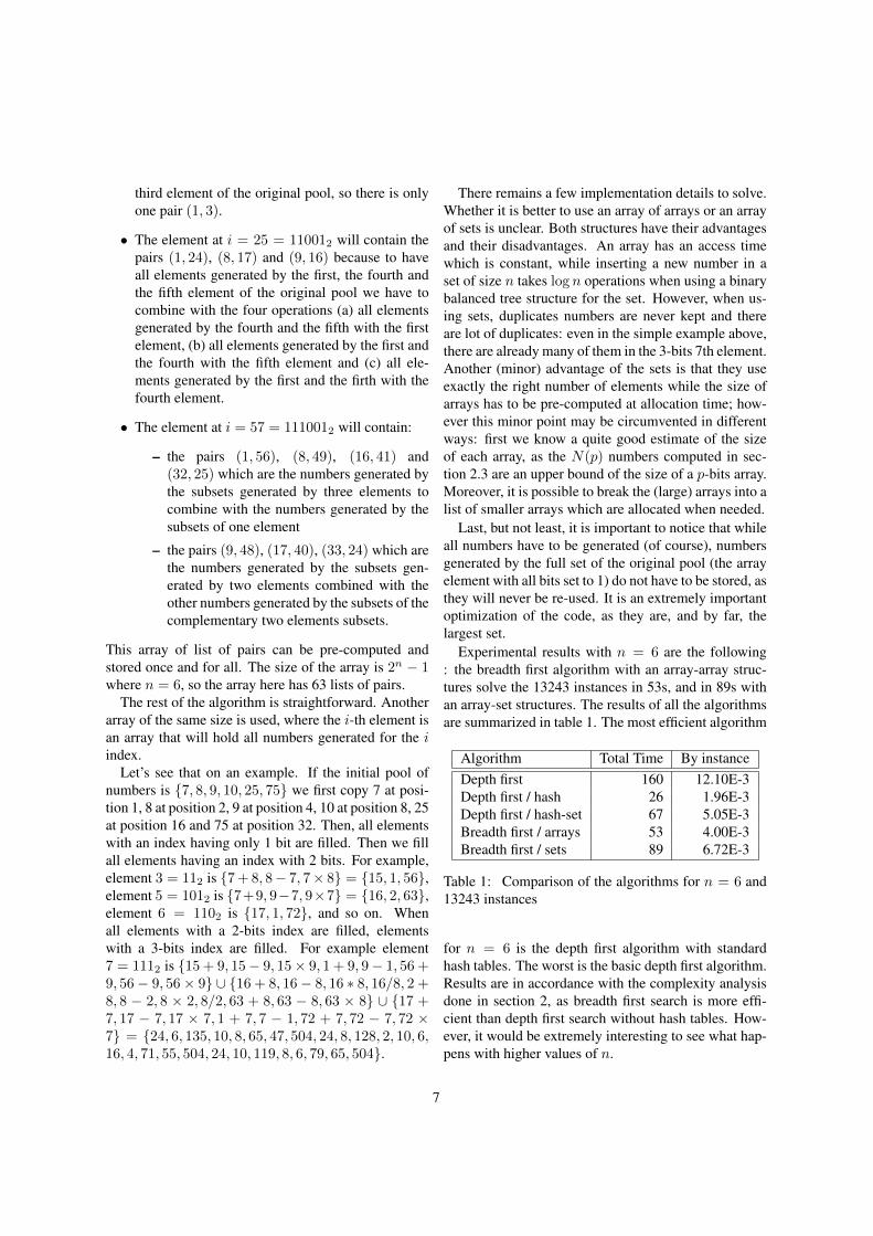
The other idea comes from the complexity studywhich provides a hint: when the size of the sets of avail-able numbers increases, the game becomes apparentlyextremely difficult. If we use the complexity formu-las of sections 2.2 and 2.3, we plot (figure 2) in bluethe log10 of the number of operations required by thedepth first algorithm and in red the same quantity forthe breadth first algorithm. The breadth first algorithmquickly becomes much more efficient than the depthfirst algorithm. However, its space complexity is alsoincreasing at almost the same rate as its time complex-ity, while the space complexity of the depth first algo-rithm remains extremely small. But these results do nottake into account the hash table effect for the depth firstalgorithm, or the set effect for the breadth first algo-rithm, which are both going to become primary factorsas the number of duplicate positions and numbers willbe much more important as there will be much moreways to compute numbers (especially small numbers)

4They should change the random number thingy so it doesn’t comeup with a really easy target number, meaning the contestants sit therelike stiffs for nearly 30 seconds Virtue [2014].

2 4 6 8 10

5

10

15

20

Figure 2: Complexity comparison. Blue: depth first.Red: breadth first

with a larger set of initial numbers. The number of gen-erated numbers is also going to increase: this meansthat to have a depth first algorithm efficient, the size ofthe hash tables has to be increased, which will take usout of the L2 and the L3 cache, and thus slow downsignificantly computations.

To compute the total number of different instances5,we can extend the formula in section 3:

Cn14 with no pair

+ C110 × Cn−2

13 with one pair+ C2

10 × Cn−412 with two pairs

+ ...

+ Ci10 × Cn−2i

14−i with i pairs+ ...

+ CE(n/2)10 C

n−2E(n/2)14−E(n/2) with E(n/2) pairs

=∑E(n/2)

i=0 Ci10 × Cn−2i

14−i

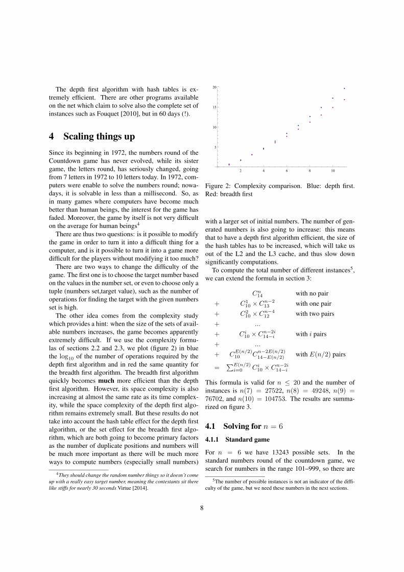
This formula is valid for n ≤ 20 and the number ofinstances is n(7) = 27522, n(8) = 49248, n(9) =76702, and n(10) = 104753. The results are summa-rized on figure 3.

4.1 Solving for n = 6

4.1.1 Standard game

For n = 6 we have 13243 possible sets. In thestandard numbers round of the countdown game, wesearch for numbers in the range 101–999, so there are

5The number of possible instances is not an indicator of the diffi-culty of the game, but we need these numbers in the next sections.

8

7 8 9 10 11 12 13

20 000

40 000

60 000

80 000

100000

120000

Figure 3: Number of instances (n = 6)

899×13243 = 11905457 possible problems. In table 2we have the distance to the closest numbers: 10858746games are solvable (91.2%), 743896 problems (6.25%)have a solution at a distance of 1 (the nearest number).

distance solved %solved cumulative0 10858746 91.21% 91.21%1 743896 6.25% 97.46%2 100517 0.84% 98.30%3 36186 0.30% 98.60%4 19387 0.16% 98.76%

Table 2: Distance to the solution

1226 instances out of 13243 (9.2%) solve all tar-get numbers in the range 101-999. One instance({1, 1, 2, 2, 3, 3}) solves none. On figure 4, we see that

0

10

20

30

40

50

60

70

80

90

100

0 100 200 300 400 500 600 700 800 900

accumulated frequencies

Figure 4: x-axis: number of numbers not found, y-axis:percentage of instances

9998 (75.5%) of the possible instances solve all possi-

ble games with less than 100 numbers missing in therange 101–999.

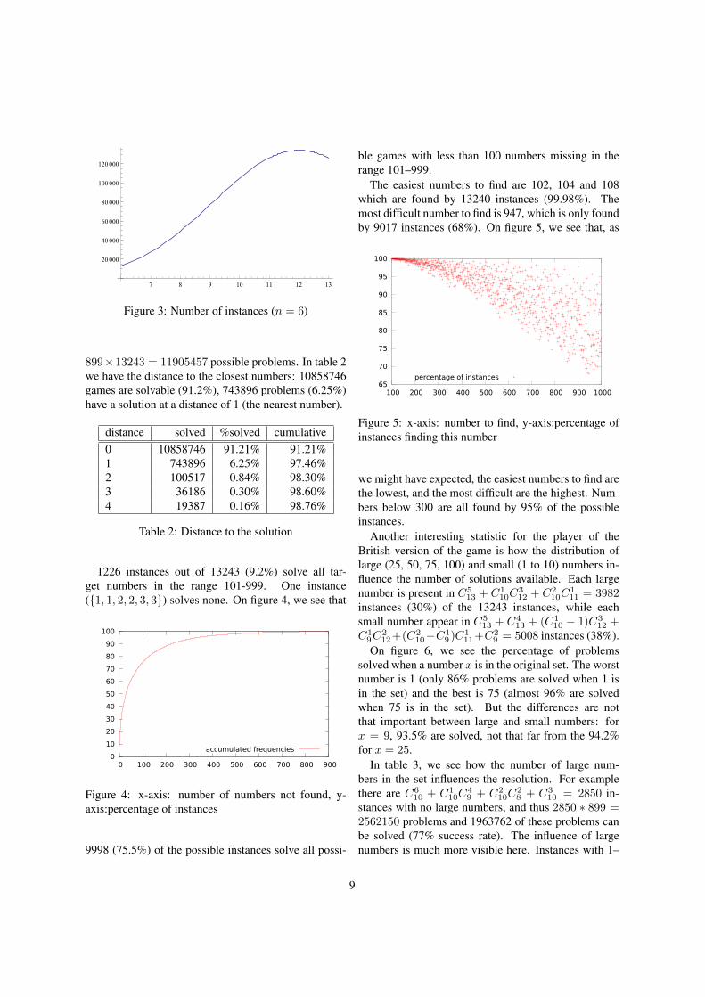
The easiest numbers to find are 102, 104 and 108which are found by 13240 instances (99.98%). Themost difficult number to find is 947, which is only foundby 9017 instances (68%). On figure 5, we see that, as

65

70

75

80

85

90

95

100

100 200 300 400 500 600 700 800 900 1000

percentage of instances

Figure 5: x-axis: number to find, y-axis:percentage ofinstances finding this number

we might have expected, the easiest numbers to find arethe lowest, and the most difficult are the highest. Num-bers below 300 are all found by 95% of the possibleinstances.

Another interesting statistic for the player of theBritish version of the game is how the distribution oflarge (25, 50, 75, 100) and small (1 to 10) numbers in-fluence the number of solutions available. Each largenumber is present in C5

13 + C110C

312 + C2

10C111 = 3982

instances (30%) of the 13243 instances, while eachsmall number appear in C5

13 + C413 + (C1

10 − 1)C312 +

C19C

212+(C2

10−C19 )C1

11+C29 = 5008 instances (38%).

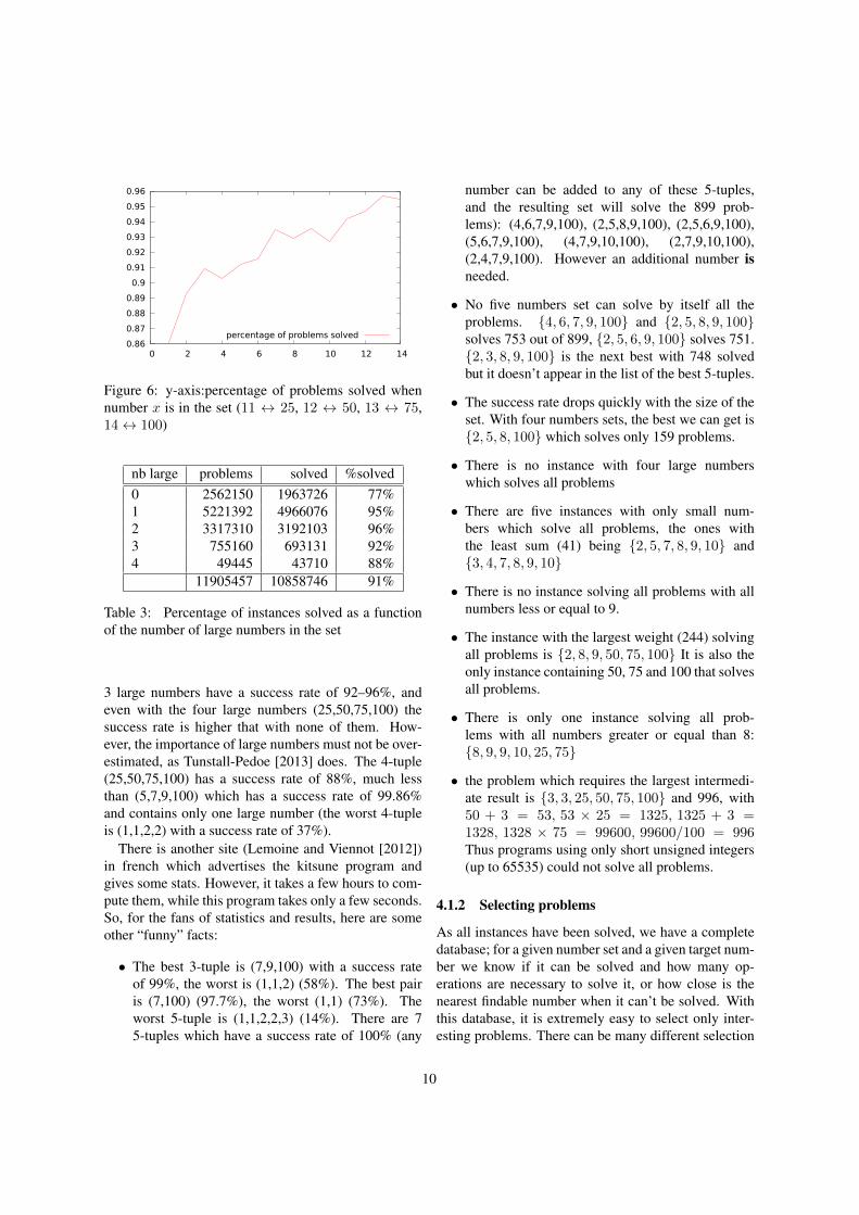
On figure 6, we see the percentage of problemssolved when a number x is in the original set. The worstnumber is 1 (only 86% problems are solved when 1 isin the set) and the best is 75 (almost 96% are solvedwhen 75 is in the set). But the differences are notthat important between large and small numbers: forx = 9, 93.5% are solved, not that far from the 94.2%for x = 25.

In table 3, we see how the number of large num-bers in the set influences the resolution. For examplethere are C6

10 + C110C

49 + C2

10C28 + C3

10 = 2850 in-stances with no large numbers, and thus 2850 ∗ 899 =2562150 problems and 1963762 of these problems canbe solved (77% success rate). The influence of largenumbers is much more visible here. Instances with 1–

9

0.86

0.87

0.88

0.89

0.9

0.91

0.92

0.93

0.94

0.95

0.96

0 2 4 6 8 10 12 14

percentage of problems solved

Figure 6: y-axis:percentage of problems solved whennumber x is in the set (11 ↔ 25, 12 ↔ 50, 13 ↔ 75,14↔ 100)

nb large problems solved %solved0 2562150 1963726 77%1 5221392 4966076 95%2 3317310 3192103 96%3 755160 693131 92%4 49445 43710 88%

11905457 10858746 91%

Table 3: Percentage of instances solved as a functionof the number of large numbers in the set

3 large numbers have a success rate of 92–96%, andeven with the four large numbers (25,50,75,100) thesuccess rate is higher that with none of them. How-ever, the importance of large numbers must not be over-estimated, as Tunstall-Pedoe [2013] does. The 4-tuple(25,50,75,100) has a success rate of 88%, much lessthan (5,7,9,100) which has a success rate of 99.86%and contains only one large number (the worst 4-tupleis (1,1,2,2) with a success rate of 37%).

There is another site (Lemoine and Viennot [2012])in french which advertises the kitsune program andgives some stats. However, it takes a few hours to com-pute them, while this program takes only a few seconds.So, for the fans of statistics and results, here are someother “funny” facts:

• The best 3-tuple is (7,9,100) with a success rateof 99%, the worst is (1,1,2) (58%). The best pairis (7,100) (97.7%), the worst (1,1) (73%). Theworst 5-tuple is (1,1,2,2,3) (14%). There are 75-tuples which have a success rate of 100% (any

number can be added to any of these 5-tuples,and the resulting set will solve the 899 prob-lems): (4,6,7,9,100), (2,5,8,9,100), (2,5,6,9,100),(5,6,7,9,100), (4,7,9,10,100), (2,7,9,10,100),(2,4,7,9,100). However an additional number isneeded.

• No five numbers set can solve by itself all theproblems. {4, 6, 7, 9, 100} and {2, 5, 8, 9, 100}solves 753 out of 899, {2, 5, 6, 9, 100} solves 751.{2, 3, 8, 9, 100} is the next best with 748 solvedbut it doesn’t appear in the list of the best 5-tuples.

• The success rate drops quickly with the size of theset. With four numbers sets, the best we can get is{2, 5, 8, 100} which solves only 159 problems.

• There is no instance with four large numberswhich solves all problems

• There are five instances with only small num-bers which solve all problems, the ones withthe least sum (41) being {2, 5, 7, 8, 9, 10} and{3, 4, 7, 8, 9, 10}

• There is no instance solving all problems with allnumbers less or equal to 9.

• The instance with the largest weight (244) solvingall problems is {2, 8, 9, 50, 75, 100} It is also theonly instance containing 50, 75 and 100 that solvesall problems.

• There is only one instance solving all prob-lems with all numbers greater or equal than 8:{8, 9, 9, 10, 25, 75}

• the problem which requires the largest intermedi-ate result is {3, 3, 25, 50, 75, 100} and 996, with50 + 3 = 53, 53 × 25 = 1325, 1325 + 3 =1328, 1328 × 75 = 99600, 99600/100 = 996Thus programs using only short unsigned integers(up to 65535) could not solve all problems.

4.1.2 Selecting problems

As all instances have been solved, we have a completedatabase; for a given number set and a given target num-ber we know if it can be solved and how many op-erations are necessary to solve it, or how close is thenearest findable number when it can’t be solved. Withthis database, it is extremely easy to select only inter-esting problems. There can be many different selection

10

criteria: solvable problems requiring more than 4 (or5...) operations, or unsolvable problems with the near-est number at a minimal given distance, or unsolvableproblems with the nearest number requiring more than4 operations, etc. . . This would turn the number roundin something worth watching again.

4.1.3 Using a larger set to pick numbers

Another way to make the game harder would be touse all available numbers between 1 and 100 whenpicking the set. Building the full database is muchmore computing intensive. In the standard game wehave 13243 sets, when picking k numbers between1 and n (including repetitions) we have Ck

n+k−1 =C6

100+6−1 = 1609344100 ' 1.6 109 possible sets, and1446800345900 ' 1.4 1012 problems. Building thedatabase took 12 hours on the cluster described in sec-tion 3.

Table 4 gives the distance to the solution, as table 2does for the standard game. Percentages are similar tothe standard problem.

dist solved %solved cumulative0 1329106855477 91.86% 91.86%1 105091143229 7.26% 99.12%2 8508187551 0.59% 99.71%3 2112923902 0.14% 99.85%4 808768195 0.06% 99.91%

Table 4: Distance to the solution

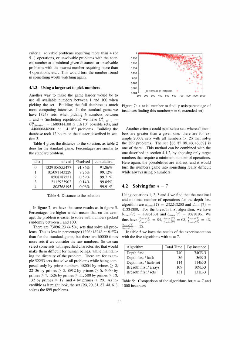
In figure 7, we have the same results as in figure 5.Percentages are higher which means that on the aver-age, the problem is easier to solve with numbers pickedrandomly between 1 and 100.

There are 73096123 (4.5%) sets that solve all prob-lems. This is less in percentage (1226/13243 ' 9.2%)than for the standard game, but there are 60000 timesmore sets if we consider the raw numbers. So we canselect some sets with specified characteristic that wouldmake them difficult for human beings, while maintain-ing the diversity of the problem. There are for exam-ple 52253 sets that solve all problems while being com-posed only by prime numbers, 48004 by primes ≥ 2,22136 by primes ≥ 3, 8912 by primes ≥ 5, 4060 byprimes≥ 7, 1526 by primes≥ 11, 500 by primes≥ 13,132 by primes ≥ 17, and 4 by primes ≥ 23. As in-credible as it might look, the set {23, 29, 31, 37, 43, 61}solves the 899 problems.

0.984

0.986

0.988

0.99

0.992

0.994

0.996

0.998

1

100 200 300 400 500 600 700 800 900 1000

percentage of instances

Figure 7: x-axis: number to find, y-axis:percentage ofinstances finding this number(n = 6, extended set)

Another criteria could be to select sets where all num-bers are greater than a given one; there are for ex-ample 20602 sets with all numbers > 25 that solvethe 899 problems. The set {35, 37, 38, 43, 45, 59} isone of them. . . This method can be combined with theone described in section 4.1.2, by choosing only targetnumbers that require a minimum number of operations.Here again, the possibilities are endless, and it wouldturn the numbers game into something really difficultwhile always using 6 numbers.

4.2 Solving for n = 7

Using equations 1, 2, 3 and 4 we find that the maximaland minimal number of operations for the depth firstalgorithm are dmax(7) = 232243200 and dmin(7) =41334300. For the breadth first algorithm, we havebmax(7) = 49951531 and bmin(7) = 9379195. Wethus have dmax(7)

dmax(6)= 84, dmin(7)

dmin(6)= 63, bmax(7)

bmax(6)= 43,

bmin(7)bmin(6)

= 32.In table 5 we have the results of the experimentation

with the five algorithms with n = 7.

Algorithm Total Time By instanceDepth first 740 740E-3Depth first / hash 36 36E-3Depth first / hash-set 114 114E-3Breadth first / arrays 109 109E-3Breadth first / sets 131 131E-3

Table 5: Comparison of the algorithms for n = 7 and1000 instances

11

We see that with the depth first algorithm, the time forsolving instances with 7 numbers is 62 (740/12) timeslarger than with n = 6. This is completely compatiblewith the minimal complexity of this algorithm, whichpredicts a ratio of 63.

With the breadth first algorithm, the time for solv-ing instances with 7 numbers is 28 (109/4) times largerthan with n = 6. This is slightly less than what wasexpected (a ratio of 32) but remains in line with whatwas expected.

With the depth first algorithm with hash table, the ra-tio is only 18. Hash tables are getting more and moreefficient, as small numbers are generated more often.An analysis of the optimal size of the hash table showsthat the best size is around 219 instead of 215 for 6 num-bers: more space is needed to hold more numbers, evenif data can not remain inside the L2 cache.

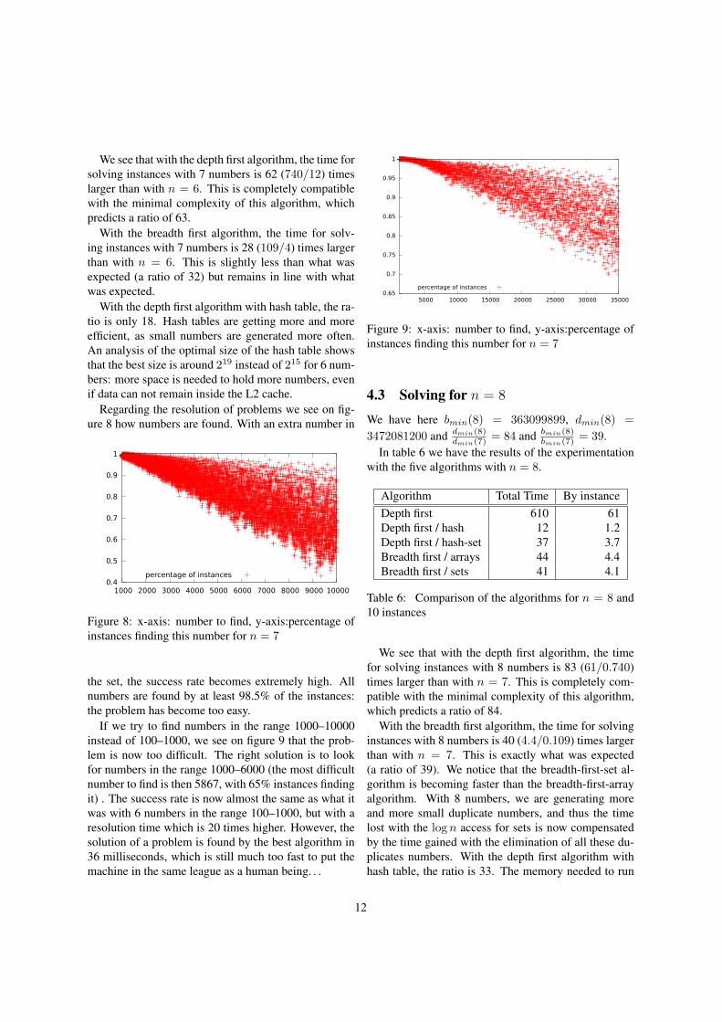
Regarding the resolution of problems we see on fig-ure 8 how numbers are found. With an extra number in

0.4

0.5

0.6

0.7

0.8

0.9

1

1000 2000 3000 4000 5000 6000 7000 8000 9000 10000

percentage of instances

Figure 8: x-axis: number to find, y-axis:percentage ofinstances finding this number for n = 7

the set, the success rate becomes extremely high. Allnumbers are found by at least 98.5% of the instances:the problem has become too easy.

If we try to find numbers in the range 1000–10000instead of 100–1000, we see on figure 9 that the prob-lem is now too difficult. The right solution is to lookfor numbers in the range 1000–6000 (the most difficultnumber to find is then 5867, with 65% instances findingit) . The success rate is now almost the same as what itwas with 6 numbers in the range 100–1000, but with aresolution time which is 20 times higher. However, thesolution of a problem is found by the best algorithm in36 milliseconds, which is still much too fast to put themachine in the same league as a human being. . .

0.65

0.7

0.75

0.8

0.85

0.9

0.95

1

5000 10000 15000 20000 25000 30000 35000

percentage of instances

Figure 9: x-axis: number to find, y-axis:percentage ofinstances finding this number for n = 7

4.3 Solving for n = 8

We have here bmin(8) = 363099899, dmin(8) =

3472081200 and dmin(8)dmin(7)

= 84 and bmin(8)bmin(7)

= 39.In table 6 we have the results of the experimentation

with the five algorithms with n = 8.

Algorithm Total Time By instanceDepth first 610 61Depth first / hash 12 1.2Depth first / hash-set 37 3.7Breadth first / arrays 44 4.4Breadth first / sets 41 4.1

Table 6: Comparison of the algorithms for n = 8 and10 instances

We see that with the depth first algorithm, the timefor solving instances with 8 numbers is 83 (61/0.740)times larger than with n = 7. This is completely com-patible with the minimal complexity of this algorithm,which predicts a ratio of 84.

With the breadth first algorithm, the time for solvinginstances with 8 numbers is 40 (4.4/0.109) times largerthan with n = 7. This is exactly what was expected(a ratio of 39). We notice that the breadth-first-set al-gorithm is becoming faster than the breadth-first-arrayalgorithm. With 8 numbers, we are generating moreand more small duplicate numbers, and thus the timelost with the log n access for sets is now compensatedby the time gained with the elimination of all these du-plicates numbers. With the depth first algorithm withhash table, the ratio is 33. The memory needed to run

12

the breadth-first-array algorithm is 1.5Gb. The breadth-first-set algorithm still has small memory requirements.For the depth-first with hash, the optimal value of thesize of the hash table is around 223 elements.

The results are presented in figure 10. Computationtook a few hours. There again, with an additional num-

0.65

0.7

0.75

0.8

0.85

0.9

0.95

1

20000 40000 60000 80000 100000 120000 140000 160000 180000 200000

percentage of instances

Figure 10: x-axis: number to find, y-axis:percentage ofinstances finding this number for n = 8 (sampled every9 points)

ber, the problem becomes too easy to solve in the pre-vious range (1000–10000). The correct range must beextended up to 35000 as we have then roughly the samemean success rate as with the standard game (the mostdifficult number to find is 34763 with a success rate of66%). However, if the depth first program is now un-able to compute the solution in less than 30s (Englishgame) or 45s (french game), the depth-first with hashstill finds a solution in 1.2s on the average.

4.4 Solving for n = 9

We have dmin(9)dmin(8)

= 108 and bmin(9)bmin(8)

= 48. Thus thestandard depth first algorithm should take more than6000s to solve a single instance and the breadth first al-gorithm with arrays should need around 40Gb of mem-ory, that the computer used for these tests don’t have.

In table 7 we have the results of the experimentationwith three algorithms with n = 9. The depth first al-gorithm wasn’t, as expected, able to solve even a singleinstance in less than 1 hour. The breadth first algorithmwith arrays generated an “Out of memory” error.

The results are presented in figure 11. We have toextend the range up to around 200000 (the most difficultnumber to find is 190667 with a success rate of 66%).Computing complete results took 3 days.

Algorithm Total Time By instanceDepth first - -Depth first / hash 147 14.7Depth first / hash-set 543 54.3Breadth first / arrays - -Breadth first / sets 467 46.7

Table 7: Comparison of the algorithms for n = 9 and10 instances

0.65

0.7

0.75

0.8

0.85

0.9

0.95

1

0 200000 400000 600000 800000 1e+06 1.2e+06 1.4e+06

percentage of instances

Figure 11: x-axis: number to find, y-axis:percentage ofinstances finding this number for n = 9 (sampled every37 points)

4.5 Solving for n = 10

For n = 10 we are at last entering uncharted territory.The average time to solve one instance of the problemseems to be around 1 to 3 minutes, so it seems impossi-ble to use an exhaustive algorithm. We are at last backin the heuristics land.

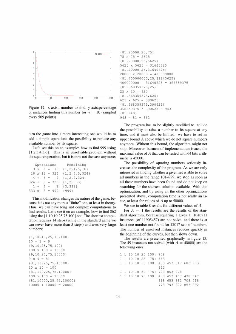
The results are presented in figure 12.Complete results were computed in 20 hours on the

cluster described in section 3. Some pools such as{5, 6, 7, 8, 9, 10, 25, 50, 75, 100} took more than onehour to complete. We had to extend the range over1000000 to have similar results regarding success rate(up to 1000000 the most difficult number to find is986189 with a 67% success rate).

5 A slightly modified problemThe problem is easy to solve because it is a finite one: ateach step, the set of available numbers is reduced by oneunit, and thus any computer program can solve it evenwith a very large set of numbers. An other solution to

13

0

1

2

3

4

5

6

7

8

0 50 100 150 200 250

nb_sols

Figure 12: x-axis: number to find, y-axis:percentageof instances finding this number for n = 10 (sampledevery 509 points)

turn the game into a more interesting one would be toadd a simple operation: the possibility to replace anyavailable number by its square.

Let’s see this on an example: how to find 999 using{1,2,3,4,5,6}. This is an unsolvable problem withoutthe square operation, but it is now not the case anymore:

Operations Remaining3 x 6 = 18 {1,2,4,5,18}

18 x 18 = 324 {1,2,4,5,324}4 + 5 = 9 {1,2,9,324}

324 + 9 = 333 {1,2,333}1 + 2 = 3 {3,333}

333 x 3 = 999 {999}

This modification changes the nature of the game, be-cause it is not any more a “finite” one, at least in theory.Thus, we can have long and complex computations tofind results. Let’s see it on an example: how to find 862using the {1,10,10,25,75,100} set. The shortest compu-tation requires 14 steps (while in the standard game wecan never have more than 5 steps) and uses very largenumbers:

{1,10,10,25,75,100}10 - 1 = 9{9,10,25,75,100}100 x 100 = 10000{9,10,25,75,10000}9 x 9 = 81{81,10,25,75,10000}10 x 10 = 100{81,100,25,75,10000}100 x 100 = 10000{81,10000,25,75,10000}10000 + 10000 = 20000

{81,20000,25,75}75 x 75 = 5625{81,20000,25,5625}5625 x 5625 = 31640625{81,20000,25,31640625}20000 x 20000 = 400000000{81,400000000,25,31640625}400000000 - 31640625 = 368359375{81,368359375,25}25 x 25 = 625{81,368359375,625}625 x 625 = 390625{81,368359375,390625}368359375 / 390625 = 943{81,943}943 - 81 = 862

The program has to be slightly modified to includethe possibility to raise a number to its square at anytime, and it must also be limited: we have to set anupper bound A above which we do not square numbersanymore. Without this bound, the algorithm might notstop. Moreover, because of implementation issues, themaximal value ofA that can be tested with 64 bits arith-metic is 45000.

The possibility of squaring numbers seriously in-creases the complexity of the program. As we are onlyinterested in finding whether a given set is able to solveall numbers in the range 101–999, we stop as soon asall these numbers have been found and do not keep onsearching for the shortest solution available. With thisoptimization, and by using all the other optimizationspresented above, computation time is not really an is-sue, at least for values of A up to 50000.

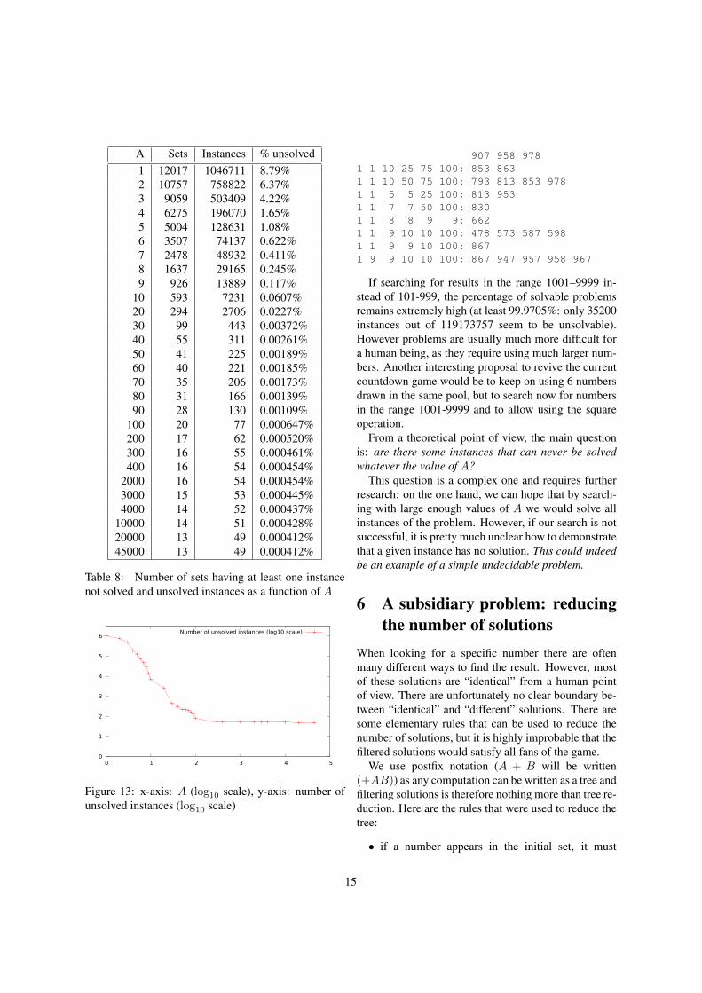
We see in table 8 results for different values of A.For A = 1 the results are the results of the stan-

dard algorithm, because squaring 1 gives 1: 1046711instances (of 11905457) are not solve, and there is atleast one number not found for 12017 sets of numbers.The number of unsolved instances reduces quickly inthe beginning of the curves, but then slows down.

The results are presented graphically in figure 13.The 49 instances not solved (with A = 45000) are thefollowing ones:

1 1 10 10 25 100: 8581 1 10 10 25 75: 8631 1 10 10 50 100: 433 453 547 683 773

8531 1 10 10 50 75: 793 853 9781 1 10 10 75 100: 433 453 457 478 547

618 653 682 708 718778 793 822 853 892

14

A Sets Instances % unsolved1 12017 1046711 8.79%2 10757 758822 6.37%3 9059 503409 4.22%4 6275 196070 1.65%5 5004 128631 1.08%6 3507 74137 0.622%7 2478 48932 0.411%8 1637 29165 0.245%9 926 13889 0.117%

10 593 7231 0.0607%20 294 2706 0.0227%30 99 443 0.00372%40 55 311 0.00261%50 41 225 0.00189%60 40 221 0.00185%70 35 206 0.00173%80 31 166 0.00139%90 28 130 0.00109%

100 20 77 0.000647%200 17 62 0.000520%300 16 55 0.000461%400 16 54 0.000454%

2000 16 54 0.000454%3000 15 53 0.000445%4000 14 52 0.000437%

10000 14 51 0.000428%20000 13 49 0.000412%45000 13 49 0.000412%

Table 8: Number of sets having at least one instancenot solved and unsolved instances as a function of A

0

1

2

3

4

5

6

0 1 2 3 4 5

Number of unsolved instances (log10 scale)

Figure 13: x-axis: A (log10 scale), y-axis: number ofunsolved instances (log10 scale)

907 958 9781 1 10 25 75 100: 853 8631 1 10 50 75 100: 793 813 853 9781 1 5 5 25 100: 813 9531 1 7 7 50 100: 8301 1 8 8 9 9: 6621 1 9 10 10 100: 478 573 587 5981 1 9 9 10 100: 8671 9 9 10 10 100: 867 947 957 958 967

If searching for results in the range 1001–9999 in-stead of 101-999, the percentage of solvable problemsremains extremely high (at least 99.9705%: only 35200instances out of 119173757 seem to be unsolvable).However problems are usually much more difficult fora human being, as they require using much larger num-bers. Another interesting proposal to revive the currentcountdown game would be to keep on using 6 numbersdrawn in the same pool, but to search now for numbersin the range 1001-9999 and to allow using the squareoperation.

From a theoretical point of view, the main questionis: are there some instances that can never be solvedwhatever the value of A?

This question is a complex one and requires furtherresearch: on the one hand, we can hope that by search-ing with large enough values of A we would solve allinstances of the problem. However, if our search is notsuccessful, it is pretty much unclear how to demonstratethat a given instance has no solution. This could indeedbe an example of a simple undecidable problem.

6 A subsidiary problem: reducingthe number of solutions

When looking for a specific number there are oftenmany different ways to find the result. However, mostof these solutions are “identical” from a human pointof view. There are unfortunately no clear boundary be-tween “identical” and “different” solutions. There aresome elementary rules that can be used to reduce thenumber of solutions, but it is highly improbable that thefiltered solutions would satisfy all fans of the game.

We use postfix notation (A + B will be written(+AB)) as any computation can be written as a tree andfiltering solutions is therefore nothing more than tree re-duction. Here are the rules that were used to reduce thetree:

• if a number appears in the initial set, it must

15

be used rather than built. For example, if wehave {2, 3, 5, 100}, finding 500 must be done by(∗ 5 100) and not (∗ (+ 2 3) 100)

• (+ A B) and (+ B A) are identical.

• (∗ A B) and (∗ B A) are identical. These tworules have to be checked recursively.

• (∗ A 1) and (/ A 1) are A

• (+ A 0) and (− A 0) are A

• A general reduction rule must be applied to allsubtrees that contain only + and − operations toput them in a “canonical” form. For example(+ (+ 1 4) (− 6 (+ 3 2))) must be reduced to6. The algorithm collects all “positive” numbersin one list and all “negative” numbers in anotherlist, then suppress all equal numbers or all com-binations of numbers equal in both lists, and thenconstructs a canonical tree by keeping always thesmallest positive results in the computation.

• The same rule applies to subtrees with only ∗ and/.

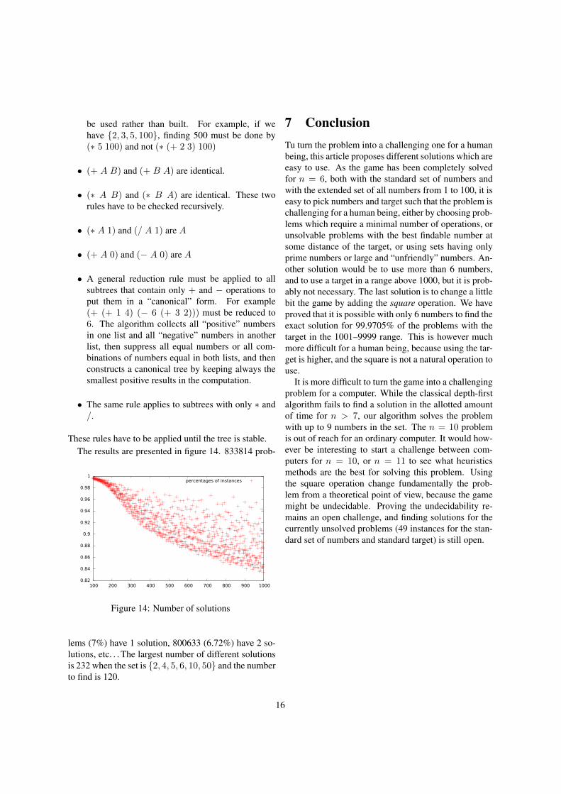
These rules have to be applied until the tree is stable.The results are presented in figure 14. 833814 prob-

0.82

0.84

0.86

0.88

0.9

0.92

0.94

0.96

0.98

1

100 200 300 400 500 600 700 800 900 1000

percentages of instances

Figure 14: Number of solutions

lems (7%) have 1 solution, 800633 (6.72%) have 2 so-lutions, etc. . . The largest number of different solutionsis 232 when the set is {2, 4, 5, 6, 10, 50} and the numberto find is 120.

7 ConclusionTu turn the problem into a challenging one for a humanbeing, this article proposes different solutions which areeasy to use. As the game has been completely solvedfor n = 6, both with the standard set of numbers andwith the extended set of all numbers from 1 to 100, it iseasy to pick numbers and target such that the problem ischallenging for a human being, either by choosing prob-lems which require a minimal number of operations, orunsolvable problems with the best findable number atsome distance of the target, or using sets having onlyprime numbers or large and “unfriendly” numbers. An-other solution would be to use more than 6 numbers,and to use a target in a range above 1000, but it is prob-ably not necessary. The last solution is to change a littlebit the game by adding the square operation. We haveproved that it is possible with only 6 numbers to find theexact solution for 99.9705% of the problems with thetarget in the 1001–9999 range. This is however muchmore difficult for a human being, because using the tar-get is higher, and the square is not a natural operation touse.

It is more difficult to turn the game into a challengingproblem for a computer. While the classical depth-firstalgorithm fails to find a solution in the allotted amountof time for n > 7, our algorithm solves the problemwith up to 9 numbers in the set. The n = 10 problemis out of reach for an ordinary computer. It would how-ever be interesting to start a challenge between com-puters for n = 10, or n = 11 to see what heuristicsmethods are the best for solving this problem. Usingthe square operation change fundamentally the prob-lem from a theoretical point of view, because the gamemight be undecidable. Proving the undecidability re-mains an open challenge, and finding solutions for thecurrently unsolved problems (49 instances for the stan-dard set of numbers and standard target) is still open.

16

ReferencesJean-Marc Alliot. Une resolution exhaustive du

”compte est bon”. Communication au groupe desutilisateurs francais de l’Amiga, 1986.

MPI board. Mpi-2, 1997. URL http://www.mcs.anl.gov/research/projects/mpi/mpi-standard/mpi-report-2.0/mpi2-report.htm.

Jean-Christophe Buisson. A moi compte, deux mots!L’ordinateur individuel, 20, 1980.

Daniel Defays. Numbo: A study in cognition andrecognition. The Journal for the Integrated Study ofArtificial Intelligence, Cognitive Science and AppliedEpistemology, 7(2):217–243, 1990.

Daniel Defays. Numbo: A study in cognition andrecognition. In Douglas Hofstadter, editor, Fluidconcepts and creative analogies: computer modelsof the fundamental mechanisms of thought. Basic-Books, 1995a.

Daniel Defays. L’esprit en friche: les foisonnementsde l’Intelligence Artificielle. Pierre Mardaga, 1995b.ISBN: 2-87009-326-8.

Patrice Fouquet. Le compte est bon, March 2010. URLhttp://patquoi.free.fr/lcpdb/.

Marc Froissart. Le compte est bon. SVM, 2:58, 1984.

INRIA. Ocaml, 2004. URL http://caml.inria.fr/ocaml/index.en.html.

Julien Lemoine and Simon Viennot. Kitsune,2012. URL http://kitsune.tuxfamily.org/wiki/doku.php.

David Levinthal. Performance analysis guide for intelcore i7 processor and intel xeon 5500 processors. In-tel report, INTEL Corporation, 2009.

Jacky Mochel. Le compte est bon, April 2003. URLhttp://j.mochel.free.fr/comptebon.php.

Jean-Eric Pin. Le compte est bon. Sujets de projets 97-98 de tronc commun informatique de l’Ecole Poly-technique de Paris, June 1998. Institution: Labora-toire d’Informatique Algorithmique: Fondements etApplications.

Williams Tunstall-Pedoe. Number games solver faq,2013. URL http://www.crosswordtools.com/numbers-game/faq.php#stats.

G. Virtue. Countdown is 70: Three cheers for the na-tion’s favourite comfort blanket. The Guardian, Jan-uary 7th 2014.

Wikipedia. Countdown (game show), 2015.URL http://en.wikipedia.org/wiki/Countdown_(game_show).

Albert L. Zobrist. A new hashing method with appli-cation for game playing. Technical report 88, Uni-versity of Wisconsin, Computer Science Department,April 1970.

17