THE FEDERAL RESERVE BANK OF ST. LOUIS CENTRAL TO AMERICA

A Quarterly Review of Business and Economic Conditions

Vol. 20, No. 1

January 2012

THE FEDERAL RESERVE BANK OF ST. LOUIS CENTRAL TO AMERICA’S ECONOMY®

The Recovery Don’t Read Too Much into “Soft Patches”

Emerging MarketsNot Just a Destination for Capital, but a Source of It

The Role of Financing in International Trade

during Good Times and Bad

c o n t e n t s

Financing International TradeBy Silvio Contessi and Francesca de Nicola

The collapse of trade during the financial crisis can be tied, for the most part, to a drop in demand. Less talked about, however, is the role of financing—or the lack thereof. In this article, learn how trade is financed and what caused such financing to plummet three years ago.

4The RegionalEconomistjanuary 2012 | VOL. 20, NO. 1

3 p r e s i d e N t ’ s m e s s a g e

1 0 Emerging Markets: a Source of and Destination for Capital

By Bryan Noeth and Rajdeep Sengupta

Increasingly, emerging markets are becoming a source of growth in the global economy. For example, foreign direct invest-ment both into and out of these countries has shown a phenom-enal increase since 2000.

12 On the road to recovery, Soft Patches Turn up Often

By Richard G. Anderson and Yang Liu

Three things to know about soft patches: There is no universally accepted definition. They are not always harbingers of the next recession. They turn up often during recoveries.

14 Starting a Business during a recoveryBy Constanza S. Liborio and Juan M. Sánchez

Businesses are always being started and shut down, creating jobs and destroying them. After previous recessions, startups exceeded closures during the recovery phase. But this time, it’s different.

16 d i s t r i c t O V e r V i e w

Local Housing Crisis Is Similar to nation’sBy Maria E. Canonand Mingyu Chen

The housing crisis in the District has been similar to that in the nation, although a bit milder. In both cases, prices today are far off their peak of about five years ago. However, the change in prices isn’t as dramatic if sales of distressed homes are excluded.

18 c O m m u N i t y p r O f i L e

Grenada, Miss.

By Susan C. Thomson

Even as the number of people who work in manufacturing continues to shrink nationwide, this tiny town in northern Mississippi continues to show blue-collar strength. About a third of its work force is employed in manufacturing.

2 1 ecONOmy at a gLaNce

2 2 N at i O N a L O V e r V i e w

The Economy Should Be able To avoid a recession in 2012By Kevin L. Kliesen

Toward the end of 2011, the economy picked up steam, albeit modestly. Further strengthening is expected this year despite high unemployment, weak household income growth and a housing market saddled with too many homes for sale.

2 3 reader exchaNge

The Regional Economist is published quarterly by the research and public affairs departments of the federal reserve Bank of st. Louis. it addresses the national, inter-national and regional economic issues of the day, particularly as they apply to states in the eighth federal reserve district. Views expressed are not necessarily those of the st. Louis fed or of the federal reserve system.

Director of Researchchristopher J. waller

senior Policy Advisercletus c. coughlin

Deputy Director of Researchdavid c. wheelock

Director of Public AffairsKaren Branding

editorsubhayu Bandyopadhyay

Managing editoral stamborski

Art DirectorJoni williams

the eighth Federal Reserve District includes all of arkansas, eastern missouri, southern illinois and indiana, western Kentucky and tennessee, and northern mississippi. the eighth district offices are in Little rock, Louisville, memphis and st. Louis.

A Quarterly Review of Business and Economic Conditions

Vol. 20, No. 1

January 2012

THE FEDERAL RESERVE BANK OF ST. LOUIS CENTRAL TO AMERICA’S ECONOMY®

The Recovery Don’t Read Too Much into “Soft Patches”

Emerging MarketsNot Just a Destination for Capital, but a Source of It



Cover: © Get ty imaGes

Please direct your comments

to subhayu Bandyopadhyay

at 314-444-7425 or by e-mail at

[email protected].

You can also write to him at the

address below. submission of a

letter to the editor gives us the right

to post it to our web site and/or

publish it in The Regional Economist

unless the writer states otherwise.

We reserve the right to edit letters

for clarity and length.

single-copy subscriptions are free

but available only to those with

U.s. addresses. to subscribe, e-mail

[email protected] or sign up

via www.stlouisfed.org/publications

You can also write to The Regional

Economist, Public Affairs office,

Federal Reserve Bank of st. Louis,

Box 442, st. Louis, Mo 63166.

ONLiNe EXTraDon’t Count On Consumer SpendingBy William R. Emmons

Consumer spending has long been the engine of U.S. and global economic growth. But five trends in 2011 suggest that such spending can no longer be counted on. Finding a replacement is going to be difficult, at best. Read this article at www.stlouisfed.org/publications/re

2 The Regional Economist | january 2012

ccording to the National Bureau of Economic Research, the Great Reces-sion officially began during the fourth quarter of 2007 (December 2007) and ended during the second quarter of 2009 (June 2009). Subsequently, the U.S. economy has recovered slowly, despite many policy actions aimed at stimulating economic activ-ity. Given the financial crisis, as well as the apparent real estate bubble and its subsequent collapse during the 2000s, the pace of the recovery is not surprising, especially when one looks at investment data. This raises questions about how we should be evaluating the current economy’s performance.

If we define recovery as real (i.e., inflation-adjusted) gross domestic product (GDP) hav-ing surpassed its previous peak level, which happened in the third quarter of 2011, then the economy has recovered from the reces-sion. Most of the major components of real GDP have also recovered to their levels dur-ing the previous peak. On the consumption side, real personal consumption expenditures are actually higher now than they have ever been. In addition, real government expen-ditures are higher than their 2007:Q4 level, despite the fact that state and local govern-ment spending has been declining in recent years. Real exports are higher as well, while real imports are roughly the same as they were in 2007:Q4.

The glaring exception in the recovery, how-ever, involves the path of investment spending. Real private investment remains roughly 16 percent below its level during the previous business cycle peak. If investment had recov-ered to the extent that consumption has, GDP would have been an estimated 4.4 percent (or nearly $670 billion in current dollars) higher in 2011:Q3 than the actual data show.1

Within investment, the components that have not recovered are those related to real estate. In 2011:Q3, real private residential investment (the housing side) was 38 percent lower and real private nonresidential invest-ment in structures (the commercial side) was

28 percent lower than their 2007:Q4 levels. These two components declined during the 2007-09 recession and have simply remained low. Real investment in equipment and soft-ware, on the other hand, was 2 percent higher in 2011:Q3 than its previous peak level. Col-lectively, these data support the view that a real estate bubble collapsed.

The U.S. economy experienced overin-vestment in housing that was driven to a significant degree by beliefs that housing prices would continue to rise. As a result, too many resources were allocated to the housing sector, creating a bubble that lasted from roughly 2001 to 2007. The effects were not limited to the housing sector, though; extra resources also went to businesses that support that sector, such as those in manufacturing, transportation and retail. Consequently, GDP temporarily grew more rapidly during this period than it otherwise would have. The rapid growth was ultimately unsustainable: The bubble burst and led to a large recession.

In the aftermath of the collapsed bubble, it is not reasonable to expect economic output and, in particular, the components of investment related to housing to return quickly to their previous business cycle peak levels. Because of the overinvestment during the 2000s, the U.S. economy now has high inventories of houses and commercial real estate. Given this overabundance, it will take time and economic growth before substantial amounts of new investment in houses and commercial real estate occur.

In general, 2007:Q4 should not be used as the benchmark for where the economy is supposed to be now, precisely because part of the economic activity during the previous decade was due to artificial growth driven by a bubble. A more appropriate assessment of today’s economic performance would focus on underlying trend growth, thereby excluding growth caused by the bubble. To illustrate, real GDP grew at an annual rate of 2.7 percent per quarter, on average, during

The Economic Recovery: america’s Investment Problem

E N D N O T E S

1 This estimate was based on my own calculation. The Bureau of Economic Analysis provides data on GDP and its components.

2 For more discussion, see my speeches on July 29, 2011, “Views on the U.S. Economy: A Four-Part Story,” and Sept. 26, 2011, “America’s Investment Problem and Monetary Policy.” See http://research.stlouisfed.org/econ/bullard/pdf/Bullard3rdRocky MountainEconomicSummit29July2011Final.pdf and http://research.stlouisfed.org/econ/bullard/pdf/Bullard_MGA_September26_2011_Final.pdf

3 For related reading, see Peralta-Alva, Adrian. “Construction and the Great Recession,” Economic Synopses, No. 35, 2011. Also, see Sánchez, Juan M.; and Thornton, Daniel L. “Why Is Employment Growth So Low?” Economic Synopses, No. 37, 2011. See http://research.stlouisfed.org/publications/es/11/ES1135.pdf and http://research.stlouisfed.org/publications/es/11/ES1137.pdf

the 2002-07 expansion. The nonbubble trend growth rate during that period would have been lower—for instance, 2.4 percent. This is the average growth rate since the Great Recession ended; thus, it does not include a real estate bubble. Many analyses simply compare today’s economy to where it would be had it continued to grow at the higher rate. It would be more appropriate, however, to compare today’s economy to one that grew steadily at the lower, nonbubble trend rate.

The latter comparison may still indicate that economic output remains below its potential, but it would not be as far below as the former would suggest. Which compari-son is used has important implications for monetary policy. Moreover, policymakers must be careful not to reinflate the bubble because, as we have seen, such growth is not sustainable and can lead to poor economic outcomes upon its collapse.2,3

P r e s i d e n T ’ s M e s s a g e

James Bullard, president and ceO

federal reserve Bank of st. Louis

the regional economist | www.stlouisfed.org 3

4 the regional economist | January 2012

i M P o r T s a n d e x P o r T s

© Get ty imaGes



By Silvio Contessi and Francesca de Nicola

The peak of the global financial crisis and Great Recession witnessed the largest fall in international trade since the Great Depression, as imports and

exports contracted by nearly 30 percent relative to GDP. The blue bars in Figure 1 show this drop for groups of countries during the peak of the crisis, between

October 2008 and January 2009. The collapse of trade in those months is astonishing when compared with the decline during other recessions.

Several factors are responsible for the plunge; a 2010 article in The Regional Economist discussed the likely culprits but concluded at that time that there was no one smoking gun.1 Today, there is some consensus among economists that

demand for intermediate goods (such as machinery parts and food ingredients) and durable goods (such as cars and appliances) played a large role; purchases of

these goods are relatively easy to postpone by households and firms during tough times. Research by economists Jonathan Eaton, Samuel Kortum, Brent Neiman and John Romalis attributes more than 70 percent of the decline in trade during

the Great Recession to the large drop in demand and, particularly, to the collapse of expenditures on durable goods.2 This leaves room for other factors to explain the remaining 30 percent, and many economists agree that this share is

explained, at least in part, by the collapse of trade finance during the crisis.



Why Do Exporters need Trade Finance? What Is It?

Most firms rely on external capital (as opposed to their own capital, internal cash flows and reinvested earnings) to finance fixed costs—such as research and develop-ment, advertising, fixed capital equipment—and also to finance intermediate input purchases, inventories, payments to workers and other frequent costs before sales and payments of their output take place.

As explained by economists Davin Chor and Kalina Manova, export activities entail extra upfront expenditures that may force firms to rely on external finance.3 Extra money may be needed, for example, to research the profitability of new export mar-kets; to make market-specific investments in capacity, product customization and regula-tory compliance; and to set up and maintain foreign distribution networks.

Exporting activities may also generate additional variable trade costs due to ship-ping, duties and freight insurance, some of which are incurred before export revenue is realized. In addition, cross-border delivery can take longer to complete than domes-tic orders, increasing the need for work-ing capital requirements relative to those

of firms that sell only domestically. For example, ocean transit shipping times can be as long as several weeks, during which the exporting firm typically would be wait-ing for payment.4

Accordingly, financial institutions and governments have developed instruments to provide so-called trade finance, i.e., finan-cial instruments that are used and some-times tailored to satisfy exporters’ needs. Most of these contracts require some form of collateral, e.g., tangible assets, including inventories. The role of trade finance in international trade is quantitatively impor-tant: Some estimates report that up to 90 percent of world trade relies on one or more trade finance instruments.5

Banks and other institutions provide trade finance for two purposes. First, trade finance serves as a source of working capital for individual traders and international companies in need of liquid assets. Second, trade finance provides credit insurance against the risks involved in international trade, such as price or currency fluctuations, or political risk. Each of these two func-tions is fulfilled by a certain set of credit instruments, provided mostly by financial institutions but sometimes also by govern-ment institutions.

FIGURE 1

Changes in Exports and Trade Finance between October 2008 and January 2009

sourCe: asmondson et al.

B y G r o u p s o f C o u n t r i e s ( p e r C e n t d e C l i n e )

there is a distinction between trade credit and trade finance. trade credit is an agreement whereby a customer can purchase goods on account (without paying cash), paying the supplier at a later date. usually when the goods are delivered, a trade credit is given for a specific number of days— 30, 60 or 90—and it is recorded in the accounts receivable section of the firm’s balance sheet. several firms record trade credit but are not engaged in international trade. trade finance generally refers to formal borrowing by firms from financial institutions and govern-ments to facilitate international trade activities.

–60 –40 –20 0

Latin America

Middle East and the Maghreb

Developing Asia

Emerging Asia, including China and India

Southeast Europe/Central Asia

Emerging Europe

Sub-Saharan Africa

Industrial Countries

Trade FinanceGoods Exports

Different Types of Trade Finance Instruments

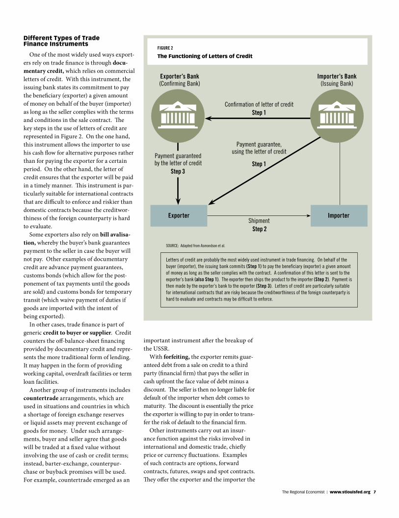
One of the most widely used ways export-ers rely on trade finance is through docu-mentary credit, which relies on commercial letters of credit. With this instrument, the issuing bank states its commitment to pay the beneficiary (exporter) a given amount of money on behalf of the buyer (importer) as long as the seller complies with the terms and conditions in the sale contract. The key steps in the use of letters of credit are represented in Figure 2. On the one hand, this instrument allows the importer to use his cash flow for alternative purposes rather than for paying the exporter for a certain period. On the other hand, the letter of credit ensures that the exporter will be paid in a timely manner. This instrument is par-ticularly suitable for international contracts that are difficult to enforce and riskier than domestic contracts because the creditwor-thiness of the foreign counterparty is hard to evaluate.

Some exporters also rely on bill avalisa-tion, whereby the buyer’s bank guarantees payment to the seller in case the buyer will not pay. Other examples of documentary credit are advance payment guarantees, customs bonds (which allow for the post-ponement of tax payments until the goods are sold) and customs bonds for temporary transit (which waive payment of duties if goods are imported with the intent of being exported).

In other cases, trade finance is part of generic credit to buyer or supplier. Credit counters the off-balance-sheet financing provided by documentary credit and repre-sents the more traditional form of lending. It may happen in the form of providing working capital, overdraft facilities or term loan facilities.

Another group of instruments includes countertrade arrangements, which are used in situations and countries in which a shortage of foreign exchange reserves or liquid assets may prevent exchange of goods for money. Under such arrange-ments, buyer and seller agree that goods will be traded at a fixed value without involving the use of cash or credit terms; instead, barter-exchange, counterpur-chase or buyback promises will be used. For example, countertrade emerged as an


Exporter’s Bank(Confirming Bank)

Exporter Importer

payment guarantee,using the letter of credit

Confirmation of letter of credit

shipment

Step 1

Step 1

Step 2

payment guaranteed by the letter of credit

Step 3

sourCe: adapted from asmondson et al.

letters of credit are probably the most widely used instrument in trade financing. on behalf of the buyer (importer), the issuing bank commits (Step 1) to pay the beneficiary (exporter) a given amount of money as long as the seller complies with the contract. a confirmation of this letter is sent to the exporter’s bank (also Step 1). the exporter then ships the product to the importer (Step 2). payment is then made by the exporter’s bank to the exporter (Step 3). letters of credit are particularly suitable for international contracts that are risky because the creditworthiness of the foreign counterparty is hard to evaluate and contracts may be difficult to enforce.

Importer’s Bank(issuing Bank)

important instrument after the breakup of the USSR.

With forfeiting, the exporter remits guar-anteed debt from a sale on credit to a third party (financial firm) that pays the seller in cash upfront the face value of debt minus a discount. The seller is then no longer liable for default of the importer when debt comes to maturity. The discount is essentially the price the exporter is willing to pay in order to trans-fer the risk of default to the financial firm.

Other instruments carry out an insur-ance function against the risks involved in international and domestic trade, chiefly price or currency fluctuations. Examples of such contracts are options, forward contracts, futures, swaps and spot contracts. They offer the exporter and the importer the

FIGURE 2

The Functioning of Letters of Credit


possibility to insure against the risk of fluc-tuations in exchange rates or prices, which would cause them a loss.

Finally, there are many situations in which instruments are provided by gov-ernments and government-related institu-tions; these types of support should also be considered part of trade finance. One such institution is the export credit insur-ance agency, also known as an investment insurance agency. These organizations act as intermediaries between national govern-ments and exporters, offering financial and

insurance services to protect trade partners against various types of risks, ranging from currency fluctuations to riots and other political distress. These agencies may pro-vide short (for up to 180 days) or long (for up to three years) term insurance to export-ers, providing exporters with the necessary credit to cover production and transporta-tion costs. Certain central banks provide refinancing schemes through which they discount the commercial bills of exporters at preferential rates; these refinancing schemes work in a way similar to forfeiting. Finally, specialized financial agencies, such as the Export-Import Bank in the U.S., specifically target exporters’ and importers’ needs.

Data on these instruments are hard to come by.6 Nevertheless, a growing body of economic research has started to provide evidence on the collective impact of these instruments on export activities. Some of this evidence precedes the recent financial crisis. Some other evidence refers to large crises, such as the recent global recession.

What’s the Evidence?

Trade economists are particularly interested in explaining why only a small percentage of firms in a country export (the economists call the number of exporters the extensive margin), in addition to explaining how much each firm exports (they call the size of individual exports the

intensive margin). Trade finance influences firms’ export status in two ways. First, it may affect the probability of a business becoming an exporter in the first place if that business needs financing to pay fixed and sunk costs in order to start export-ing. Second, trade finance may affect the magnitude of foreign sales because financ-ing variable export costs may also require external finance.

To understand how finance affects the number of exporters and the size of their sales, economist Kalina Manova exploits the fact that (i) different industries tend to rely with different intensity on external finance, and (ii) the cost and availability of credit vary across countries.7 The researcher shows that countries in which credit is either more difficult or more expensive to obtain tend to export less, especially in industries that rely more heavily on external finance. Economists Nicolas Berman and Jérôme Héricourt study the relationship between trade and finance using firm-level survey data from nine emerging and developing countries from the World Bank.8 They show that firms’ financial health raises neither the probability of remaining an exporter once the firm has entered international markets nor the size of exports. However, access to finance affects the probability of becoming an exporter. They also show that the level of financial development of a country—not just an individual firm’s access to credit—can affect the probability of starting to export.

In addition to these two studies, there are many recent contributions confirming the important role of trade finance in influenc-ing the number of exporters and how much they export. One major challenge of these studies is to avoid confusing the role of finance with the role of changes in demand for exporters’ products. This distinction is important: If banks reduce the supply of trade finance to exporters (for example, during a financial crisis), appropriate policy interventions can restore firms’ access to credit and allow exporters to continue sell-ing abroad.

A recent analysis by economists Mary Amiti and David Weinstein sheds light on the relationship between banks’ health and firms’ export performance in Japan. The Japanese banking system underwent a credit crunch in the 1990s and 2000s. Many banks

these organizations act as intermediaries between national

governments and exporters, offering financial and insurance

services to protect trade partners against various types of

risks, ranging from currency fluctuations to riots and other

political distress.

Related Reading on Trade Issues from the St. Louis Fed

The Trade collapse: lining up the suspects a two-page article co-authored

by silvio contessi in the april 2010

issue of The Regional Economist.,

see stlouisfed.org/tradecollapse

u.s. Trade springs Backa two-page essay co-authored by

contessi in april 2011 as part of our

Economic Synopses series. see

http://research.stlouisfed.org/ publications/es/11/es1109.pdf

© CorBis


had a sizable amount of bad loans on their balance sheets and had a hard time extend-ing new loans to their customers. Amiti and Weinstein matched Japanese export-ers to the Japanese banks from which they borrowed and constructed a measure of market-to-book value for all large Japanese banks. In general, as the market value of a bank fell, it had a harder time extending new loans or rolling over existing loans. The researchers showed that there was a large disparity across Japanese banks in these measures and that such large differ-ences can be exploited to estimate the effect of bank health on exports. In particular, Japanese firms that borrowed from dis-tressed banks contracted their exports much more than businesses that were borrowing from healthy banks.

Trade Finance during the Crisis

The conjecture in the aftermath of the crisis was that the tightening of credit to firms had depressed the intensive margin of exports (how much each firm can export), especially in the sectors more exposed to financial shocks arising from the financial crisis because they tend to rely more on external finance. For example, several stud-ies have shown that industries such as drugs and pharmaceuticals or plastic and comput-ing tend to use much more external finance than industries such as tobacco or pottery.

There is consensus among economists that the financial crisis led to tightened financial conditions. How much of these tightened credit conditions is specifically reflected in trade finance is difficult to assess because of the absence of data. However, a survey jointly administered by the Interna-tional Monetary Fund and the BAFT-IFSA provides some insight.9 According to a recent IMF study of this survey’s confiden-tial data, changes in trade finance condi-tions were particularly pronounced among large banks that suffered most from the financial crisis and, consequently, were in greater need to quickly deleverage.10 The survey also shows that, at the same time, banks increased the cost of borrowers. The IMF/BAFT-IFSA Trade Finance Survey provides evidence that, particularly in the case of letters of credit and trade-related lending, the terms of credit offered by large banks worsened.

The drop in trade at the peak of the crisis, between October 2008 and January 2009, is shown in Figure 1. The trade collapse was visibly much larger than the contraction in trade finance, seen in the red bars. At the onset of the crisis (2007:Q4-2008:Q4), trade finance actually increased; even during the peak of the crisis (2008:Q4-2009:Q1), trade finance fell by only one-third rela-tive to the collapse in the export of goods. There was much geographic variation, but the largest drops occurred in Central Asia and Southeastern Europe. The situation remained negative but stable in the second quarter of 2009 and started to recover by the end of 2009 when Maghreb countries (in North Africa) and Middle Eastern countries (Emerging Asia) experienced the largest increase in goods exports worldwide.

When interviewed about the perceived causes of the contraction of trade finance, the surveyed banks returned answers sur-prisingly similar to the consensus emerging among economists. Respondents identified the fall in the demand for trade activities as the major source of decline in the value of trade finance but attributed about 30 percent of the fall to the reduced credit availability at either their own institutions or counterparty bank.

Conclusion

Two of the major difficulties regarding policymaking in the area of trade finance are the lack of reliable quantitative infor-mation and the limited evidence on the relationship between international trade and trade finance. Recent research and efforts in data collection, however, are fostering the understanding of this relationship and, ulti-mately, of the potential impact of different policies that may limit the negative effects of financial crises in the future.

Silvio Contessi is an economist at the Federal Reserve Bank of St. Louis. See http://research.stlouisfed.org/econ/contessi/ for more of his work. Francesca de Nicola is a postdoctoral fellow in the Markets, Trade, and Institutions Division of the International Food Policy Research Institute in Washington, D.C.

E N D N O T E S

1 See Contessi and El-Ghazaly. 2 See Eaton et al. 3 See Chor and Manova. 4 See Hummels and Schaur. 5 See Auboin. 6 Bank trade finance is based on idiosyncratic

relationships with specific clients so that its availability and even its cost depend on a complicated relationship among client, counterparty and counterparty banks. As there is much proprietary information about bank-client relationships, this information is rarely disclosed.

7 See Manova. 8 See Berman and Héricourt. 9 BAFT-IFSA is the global financial services

association formed by the merger of the Bankers’ Association for Finance and Trade (BAFT) and the International Financial Services Association (IFSA).

10 See Asmondson et al.

R E F E R E N C E S

Amiti, Mary; and Weinstein, David E. “Exports and Financial Shocks.” National Bureau of Economic Research Working Paper No. 15556, December 2009.

Asmondson, Irena; Dorsey, Thomas; Kha-chatryan, Armine; Niculcea, Ioana; and Saito, Mika. “Trade and Trade Finance in the 2008-09 Financial Crisis.” International Monetary Fund Working Paper 11/16, January 2011.

Auboin, Marc. “Restoring Trade Finance during a Period of Financial Crisis: Stock-Taking of Recent Initiatives.” WTO Staff Working Paper ERSD-2009-16, December 2009.

Berman, Nicolas; and Héricourt, Jérôme. “Financial Factors and the Margins of Trade: Evidence from Cross-Country Firm-level Data.” Journal of Development Economics, November 2010, Vol. 93, No. 2, pp. 206-17.

Chor, Davin; and Manova, Kalina. “Off the Cliff and Back? Credit Conditions and International Trade during the Global Financial Crisis.” Journal of International Economics, forthcoming in 2012.

Contessi, Silvio; and El-Ghazaly, Hoda S. “The Trade Collapse: Lining Up the Suspects.” The Federal Reserve Bank of St. Louis’ The Regional Economist, April 2010, Vol. 18, No. 2, pp. 10-11.

Eaton, Jonathan; Kortum, Samuel; Neiman, Brent; and Romalis, John. “Trade and the Global Recession.” NBER Working Paper No. 16666, January 2011.

Hummels, David L.; and Schaur, Georg. “Hedging Price Volatility Using Fast Trans-port.” Journal of International Economics, September 2010, Vol. 82, No. 1, pp. 15-25.

Manova, Kalina. “Credit Constraints, Equity Market Liberalizations, and International Trade.” Journal of International Economics, September 2008, Vol. 76, No. 1, pp. 33-47.


Emerging markets are increasingly becoming a source of growth in the

complex global economy. Brazil, Russia, India, Indonesia, China and South Korea are projected to account for approximately 45 percent of the global output by the year 2025, up from 37 percent in 2011, according to a report from the International Monetary Fund.1

Although there are varying definitions of what precisely is an emerging market, in general, countries that experience significant growth in GDP and infrastructure are given this distinction.2 Emerging markets typically have lower per capita GDP and have enacted structural economic reforms in an effort to grow rapidly and to catch up with more-developed nations. A natural consequence of this has been the growth of capital markets and the increasing capital flows to and from these countries.

In what follows, we make a very prelimi-nary study of the trends in capital flows to and from emerging markets over the past couple of decades.

Half the World’s People

The countries on our list of emerging markets make up a sizable portion of the world’s population. They had roughly 3.6 billion inhabitants as of 2010, most of whom reside in China or India, according to population estimates from the U.N. Depart-ment of Economic and Social Affairs. This total represents about 52 percent of the global population and is expected to grow.

Before the financial crisis of 2007-2009, emerging markets had significantly higher growth rates compared with the rates in countries that belong to the Organisation for Economic Co-operation and Development

1992 1994 1996 1998 2000 2002 2004 2006 2008 2010

200180160140120100

80604020

0

16

14

12

10

8

6

4

2

0

Other Emerging

Russian Federation

India

China

Brazil

Percent of World (right axis)

BILL

IONS

$ PERCENT

sourCe: united nations Conference on trade and development.

Emerging Markets’ Outward Flows of Foreign Direct Investment

FIGURE 1

1992 1994 1996 1998 2000 2002 2004 2006 2008 2010

400

350

300

250

200

150

100

50

0

25

20

15

10

5

0

Brazil

Percent of World (right axis)

BILL

IONS

$ PERCENT

Other Emerging

Russian Federation

India

China

sourCe: united nations Conference on trade and development.

Emerging Markets’ Inward Flows of Foreign Direct Investment

FIGURE 2

(OECD), whose members are usually con-sidered to be more developed. However, the financial crisis had a large impact on both OECD countries and emerging markets. Although emerging markets as a whole wit-nessed slower growth during the downturn, they did not see a wholesale contraction in economic activity as their OECD counter-parts witnessed.

Types of Capital Flows

An engine of growth for emerging mar-kets, capital flows are typically broken into

two principal categories: foreign portfolio investment (FPI) and foreign direct invest-ment (FDI). In spirit, FPI is investment that is made without gaining a controlling interest in the entity receiving the funds. It is an investment in an asset for the purpose of earning a return (e.g., the purchase of corpo-rate or government securities or bonds). FDI entails some sort of ownership or controlling stake (e.g., investing in a factory or land). In general, the benchmark for FDI is if an investor takes at least a 10 percent controlling stake in the target entity. This essay focuses

i n T e r n a T i o n a l

emerging Markets: a source of and destination for capitalBy Bryan Noeth and Rajdeep Sengupta

© CorBis

the regional economist | www.stlouisfed.org 11the regional economist | www.stlouisfed.org 11

more attention on FDI because of its stronger links to growth and employment.

FDI cultivates development because, in addition to the resources that it provides developing economies, it gives them the opportunity to “learn by doing,” which leads to growth-enhancing innovation and spill-overs. Over the past couple of decades, the share of FDI in total foreign equity flows has been larger for developing countries than for developed countries.3 Arguably, the causality runs both ways: Those engaging in FDI are more likely to target countries with greater growth potential.

Figures 1 and 2 highlight the important trends in emerging markets’ inflows and outflows of FDI. First, the absolute values of FDI into and out of emerging markets have shown a phenomenal increase since 2000. This is just another piece of evidence of the importance of emerging markets in an increasingly globalized world. Second, within emerging markets, the relative shares of individual countries’ FDI flows have remained fairly stable. China appears to play a prime role in both the inflow and outflow of FDI. Brazil appears to be a major destination for FDI inflows, whereas Russia appears to be a major source of FDI outflows. Third, dur-ing 1993-1997, emerging markets accounted for over 20 percent of the share of global FDI inflows. The financial crisis in East Asia and the Russian Federation in 1998 saw a collapse in this share. This has been followed by a steady recovery since 2000. The share of FDI inflows into emerging markets now stands near the precrisis peak of the mid-1990s.

Other trends of global FDI flows have gained significant attention in recent years. Historically, the direction of capital flows has been from the developed nations to emerging markets. In the mid-1990s, while the share of FDI into emerging markets was in excess of 20 percent of global FDI inflows, the share of FDI outflows from emerging markets was less than 5 percent. Moreover, this share wit-nessed a decline in the aftermath of the Asian crisis. In contrast, from 2001 through 2010, emerging markets increased their global out-ward investment share from about 1 percent to about 14 percent. Advanced economies were not the only recipients of these invest-ments: Low-income countries saw increased capital flows due to the emerging economies’ presence in global capital markets.4 It is

E N D N O T E S

1 See IMF. 2 We distinguish the following countries as

emerging markets: Brazil, China, Egypt, India, Indonesia, the Philippines, Russia, South Africa, Turkey, Thailand, Poland, Peru and Malaysia. Many vendors, such as S&P, Dow Jones and FTSE, keep country lists according to their definition of emerging markets. Our choice of countries is derived from such lists by including countries that are common to most lists. Details of this selection procedure are available on request.

3 See Goldstein and Razin. 4 See Dabla-Norris et al. 5 See Goldstein and Razin.

R E F E R E N C E S

Dabla-Norris, Era; Honda, Jiro; Lahrech, Amina; and Verdier, Genevieve. “FDI Flows to Low-Income Countries: Global Drivers and Growth Implications.” IMF working paper, June 2010.

Goldstein, Itay; and Razin, Assaf. “An Informa-tion-Based Trade off Between Foreign Direct Investment and Foreign Portfolio Investment.” Journal of International Economics, Vol. 70, No. 1, 2006, pp. 271-95.

International Monetary Fund. “Global Develop-ment Horizons: Multipolarity: The New Global Economy.” 2011.

1992 1994 1996 1998 2000

200180160140120100806040200

Brazil

ChinaIndia

Russian Federation

BILL

IONS

$

2002 2004 2006 2008 2010

1992 1994 1996 1998 2000

50

40

30

20

10

0

–10

–20

Brazil

China

India

Russian Federation

BILL

IONS

$

2002 2004 2006 2008 2010

Capital Flows into BRIC Countries

FIGURE 3

f o r e i G n d i r e C t i n v e s t m e n t

f o r e i G n p o r t f o l i o i n v e s t m e n t

sourCe: World Bank.

important to note that the increase in the global percentage metric is due, in part, to the significant decrease in the outward FDI from OECD countries after the financial crisis of 2007-2008.

Volatility

Because of their direct links to factors of production, FDI is generally presumed to be less volatile in comparison with FPI. By taking a direct and controlling stake, FDI allows the investor to overcome information and control problems between managers and owners. On the other hand, FPI is viewed at times as “ownership without control.” Although this feature may not reduce the information and control problems of the FPI investor, it has important implications for the resale of the investment. Should the need arise to resell the investment, a well-informed FDI investor faces a classic lemons problem in attracting potential buyers. In contrast, the FPI stakes are relatively easier to sell— a rationale for their high volatility.5

As evidence of higher volatility, we look at the trends of inflows of FDI and FPI in four prominent emerging markets from 1992 through 2010. These are Brazil, Russia, India and China, popularly denoted by the acro-nym BRIC. (See Figure 3.) Noticeably, both FDI and FPI have witnessed strong growth since 2000 in BRIC countries. Clearly, flows of FDI slowed considerably after the U.S. financial crisis of 2007-2008, largely due to a reduction in growth projections. Impor-tantly, a sharp reversal of FPI resulted in the aftermath of the global financial crisis. Although the FPI flows have returned once again to their precrisis levels, Figure 3 shows why it is not difficult to see why FPI is considered the more volatile segment of capital flows.

Capital flows both into and out of emerg-ing markets are playing a larger role in the global marketplace. As these economies continue to grow at a rapid pace, it will be interesting to see the course charted by inflows and outflows of FDI and FPI as capi-tal markets continue to evolve.

Rajdeep Sengupta is an economist at the Federal Reserve Bank of St. Louis. See http://research.stlouisfed.org/econ/sengupta/ for more of his work. Bryan Noeth is a research associate at the Bank.


During mid-2009, the U.S. economy exited the economic contraction that

began year-end 2007 and entered into an economic recovery phase.1 Approximately two-and-a-half years later, both real GDP and consumer expenditures surpassed their prerecession peaks, although industrial pro-duction remained weak and the unemploy-ment rate exceeded 8.5 percent.2

During the recovery, as in many previous recoveries, analysts spoke of “soft spots” or “soft patches,” that is, periods when slower growth raised concern that economic activity might turn downward before reaching its previous peak, a so-called double-dip reces-sion. The terms “soft spot” and “soft patch” are found in Federal Reserve publications as early as the Board of Governors’ Annual Report for 1948 and, more recently, in publi-cations as varied as the Board of Governors’ semiannual Monetary Policy Report to the Congress, speeches by Federal Reserve offi-cials and transcripts of Federal Open Market Committee meetings. The terms also fre-quently appear in the popular press. Unfor-tunately, despite widespread usage, there is no accepted definition of a soft patch.

a Look at Five Business Cycles

Rebounds in economic activity, when measured by growth of real GDP, are seldom smooth; temporary slowdowns are common-place. These slowdowns, or soft patches, do not reliably foreshadow peaks in economic activity: During the past 60 years, there have been far more soft patches than business cycle peaks. Yet, fear is not baseless: All business cycle peaks since 1950 have been preceded by soft patches.

The paces of recovery following five recent business cycle troughs are shown in the

Business Cycle Expansion Dates

Length (quarters)

1950 Q1 – 1953 Q2 14

1954 Q3 – 1957 Q3 13

1958 Q3 – 1960 Q2 8

1961 Q2 – 1969 Q4 35

1971 Q1 – 1973 Q4 12

1975 Q2 – 1980 Q1 20

1980 Q4 – 1981 Q3 4

1983 Q1 – 1990 Q3 31

1991 Q2 – 2001 Q1 40

2002 Q1 – 2007 Q4 24

2009 Q3 – na

TaBLE 1

nBER Business Cycles since 1950

sourCe: national Bureau of economic research.

sourCes: Bureau of economic analysis and authors’ calculation.

–4 –3 –2 –1 0 1 2 3 4 5 6 7 8 9 10

1086420

–2–4–6–8

–10

1975

1982

2001

Current

1991

PERC

ENT

QUARTERS FROM RECESSION’S END

CYCLE TROUGH

Period-to-Period Real GDP Growth

FIGURE 1

e c o n o M Y

On the Road to Recovery, Soft Patches Turn up Often

By Richard G. Anderson and Yang Liu

figure. It shows the quarterly (that is, quarter-to-quarter) growth rate of real GDP, which is choppy in both business cycle expansions and contractions. Recoveries following cycle troughs in 1975, 1982 and 2007 (the current

recovery) displayed initial strong growth, fol-lowed by slowing after five quarters. Recover-ies following troughs in 1991 and 2001 were shallow, and subsequent recoveries were milder. During the first three years of the five recoveries, temporary slowdowns lasting two consecutive quarters occurred 22 times and slowdowns of three consecutive quarters happened 17 times. None of these slowdowns foreshadowed a business cycle peak in the near term (although, of course, peaks eventu-ally did occur).

Absent a widely accepted definition of a soft patch, we examined two possibilities:

(1) A soft patch occurs when the GDP growth rate during the current quarter and the immediately prior quarter (that is, the two most recent quarters) is less than during the quarter that preceded these two quarters (a two-quarter soft patch); and

(2) A soft patch occurs when the GDP growth rate during the current quarter and the two immediately prior quarters is less than during the quarter that preceded these three quarters (a three-quarter soft patch).

©CorBis

We examined the 11 business cycle expan-sions that have occurred since 1950. (Dates of the expansions are shown in Table 1.) The 10 expansions prior to the current expansion averaged 20.1 quarters in duration; the brief-est was four quarters, and the longest lasted 40 quarters.

Table 2 summarizes the analysis. Since 1950, during National Bureau of Economic Research (NBER) business cycle expan-sions, there have been 69 and 52 instances, respectively, of two- and three-quarter slowdowns (column 1). The frequency of soft patches overpredicts the frequency of business cycle peaks—there have been only 10 business cycle peaks.3 Yet, since 1950, every business cycle peak has been closely preceded by a soft patch. With respect to two-quarter soft patches, six business cycle peaks occurred during the final quarter of two-quarter soft patches (column 2, first row), and four occurred during the follow-ing quarter (column 3, first row); note that the 1973:Q4 peak was preceded uniquely by both two- and three-quarter soft patches. With respect to three-quarter soft patches, four peaks occurred during the final quarter of a three-quarter soft patch (column 2, second row), and one occurred immediately

after a three-quarter soft patch (column 3, second row). On average, two- and three-quarter soft patches have preceded the last 10 business cycle peaks by 12.5 and 12.7 quarters, respectively.

nothing Hard and Fast about Soft Patches

In brief, we find that soft patches—that is, slowdowns of real GDP growth lasting two or three quarters—are commonplace during economic expansions. Such slow-downs, however, are not reliable predictors of subsequent business cycle peaks (the start of recessions) despite approximately half of peak quarters being immediately preceded by a soft patch. Soft patches are far more numerous than cycle peaks, and the tim-ing between soft patches and cycle peaks is imprecise. Fluctuations in GDP growth are common during economic recoveries, and soft spots do not necessarily foreshadow further slowing.

Richard G. Anderson is an economist and Yang Liu is a senior research associate, both at the Federal Reserve Bank of St. Louis. See http://research.stlouisfed.org/econ/anderson/ for more of Anderson’s work.

Criterion (1)number of soft

patches

(2)Business cycle

peaks that occurred in final quarter of soft

patch

(3)Business cycle

peaks that occurred in the

first quarter following a soft

patch

(4)Business cycle

peaks that occurred in the second quarter following a soft

patch

(5)Business cycle

peaks that occurred in the third quarter

following a soft patch

Two-quarter soft patch: Growth in current and preceding quarter less than growth two quarters ago during an economic expansion

69 1953 Q2 1973 Q4 1980 Q1 1981 Q3 1990 Q3 2007 Q4

1957 Q3 1969 Q4 1973 Q4 2001 Q1

1960 Q2 1953 Q2 1980 Q1

Three-quarter soft patch: Growth in current and two preceding quarters less than growth three quarters ago during an economic expansion

52 1957 Q3 1969 Q4 1973 Q4 2001 Q1

1960 Q2 1980 Q1 1969 Q4 1990 Q3

Soft Patches and Business Cycle Peaks

TaBLE 2

note: Calculations are based on economic expansions defined in table 1 and quarterly growth rates of real Gdp as published november 2011. dates shown are business cycle peaks. Because the criteria for two- and three-quarter soft patches overlap, some peaks are preceded by both two- and three-quarter soft patches.

sourCes: Bureau of economic analysis, national Bureau of economic research and authors’ calculation.

E N D N O T E S

1 Most economic analysts accept the monthly and quarterly business cycle peak and trough dates determined by the National Bureau of Economic Research’s Business Cycle Dating Committee. The time interval from a peak to a trough typically is referred to as a recession or contraction, and the period from a trough to a peak as an expansion or recovery. See www.nber.org/cycles/main.html

2 According to data as of mid-December 2011, during 2011:Q3, real GDP regained (and slightly exceeded) its 2007:Q4 cycle peak, and during November 2010, real consumer expen-diture regained its December 2007 peak. Yet, industrial production and nonfarm private employment during November 2011 were 5.9 percent and 5.1 percent, respectively, below their December 2007 levels.

3 Data revisions also erase soft patches. In July 1996 congressional testimony, Fed Chairman Alan Greenspan discussed 1995’s soft patch. At that time, estimated GDP growth rates for 1995:Q1 to 1996:Q1 were 0.2, 0.1, 0.9, 0.1 and 0.5 percent, respectively. Current revised rates for the same period are 0.2, 0.2, 0.8, 0.7 and 0.7 percent. This article is based on published revised real GDP data as of mid-November 2011. An analysis of all soft patches based on the vintage data available at each historical date would be valuable but is beyond the scope of this analysis.

R E F E R E N C E S

Board of Governors of the Federal Reserve System. Annual Report (for 1948). June 1949. See http://fraser.stlouisfed.org/publications/arfr/issue/4992/download/82678/arfr_1948.pdf

Board of Governors of the Federal Reserve Sys-tem. Monetary Policy Report to the Congress. July 13, 2011. See www.federalreserve.gov/monetarypolicy/files/20110713_mprfull report.pdf

Federal Open Market Committee. Minutes of the meeting of May 3, 2005. See www.federalreserve.gov/monetarypolicy/files/FOMC20050503meeting.pdf

Greenspan, Alan. Testimony before the Com-mittee on Banking, Housing, and Urban Affairs, U.S. Senate, in conjunction with the Monetary Policy Report to the Congress. July 18, 1996. See www.federalreserve.gov/ boarddocs/hh/1996/july/testimony.htm

Greenspan, Alan. Testimony before the Com-mittee on Financial Services, U.S. House of Representatives, in conjunction with the Monetary Policy Report to the Congress. July 20, 2005. See www.federalreserve.gov/boarddocs/hh/2005/july/testimony.htm


©CorBis


The opening of new businesses is funda-mental for U.S. employment growth.

Businesses, small and large and of different ages, are constantly creating and destroying jobs. Profitable businesses stay in the market and expand, while the less-successful ones must consider downsizing or closing. These decisions, in turn, have a direct impact on the labor market. Amidst this job churn, it’s important to remember that new businesses are the key to net job creation.

To illustrate the importance of startups, it is useful to consider a 2009 study that used data from the Business Dynamics Statistics (BDS), an annual series of data from the U.S. Census Bureau. The researchers found that, on average in 1980-2005, private-sector startup employment accounted for 3 percent of the overall employment every year.1 This may seem like a small fraction, but it becomes substantial when compared with the 1.8 percent average annual net employment growth during the same period.2 Similarly, researchers showed in another 2009 study that the youngest firms (less than 5 years old) accounted for almost the entire net job creation in 1980-2005.3

Examining the behavior of current business openings seems important to understanding the progress of employment recovery after the Great Recession. This will be the focus of this article.

Startups and the Business Cycle

Smaller firms—which are most likely younger as well4—are found to be less sensitive than large ones to business cycle conditions. A recent study found that in recessions prior to 2007, small businesses contracted slower during recessions and expanded faster during recoveries compared

with large businesses, thus leading employ-ment out of the recession. However, the same paper, using more-recent Business Employment Dynamics (BED) data, shows the opposite behaviors during the Great Recession. Small firms were more affected than large firms in terms of job creation and destruction.5

The last recession and the current recovery, thus, present special episodes to examine. Startup formation experienced a substantial decline up to the third quarter of 2009, according to BED data, which are published quarterly by the Bureau of Labor Statistics. By the beginning of 2010, the number of businesses exiting the market returned to prerecession levels, but the entry of new businesses still lagged behind.

The experience of business births and deaths varied across the U.S. Some regions faced little recovery, while other areas experienced growth in startups. The avail-ability of state-level data on job creation and destruction allows for a regional examina-tion of the current recovery.

nation and District

BED data measure establishment births and deaths, as well as the subsequent cre-ation and destruction of jobs.6 Births and deaths of businesses do not include tem-porary shutdowns or seasonal reopenings. Thus, a business must be closed for a year to be considered as a death and not a tempo-rary shutdown. This, in turn, restricts the availability of business death data up to the beginning of 2010. Historically, the level of business births has been greater than deaths during economic recoveries. After the Great Recession, however, this process has been delayed by the slower growth of startups.

Figure 1 displays business births and deaths for the nation and the Eighth Dis-trict.7 They are normalized so that the peak previous to the Great Recession is equal to 100. The main message to take away is that the Eighth District behaves similarly to the nation, with startup growth in the District being slightly higher. This is reasonable since the District’s states account for a substantial amount of national business births—about 11.6 percent—and deaths—11.9 percent.

By 2010:Q1, business deaths fell to prere-cession levels for both the nation and the Dis-trict. Slow business formation, however, has delayed the closing of the gap between estab-lishments’ exit and entry levels. In 2010:Q4, for the nation and the District, startup levels were still 6.2 percent and 2.4 percent below the prerecession peak, respectively.

Job creation and destruction have varied across states. Figure 2 displays the relative degrees of recovery of each state in the Eighth District as measured by establishment creation and destruction (represented by red circles), as well as job creation by new busi-nesses and job destruction by businesses that have shut down (represented by blue squares). The horizontal axis shows the percent change from 2007:Q4 to 2010:Q1 of business forma-tion and the employment generated by those startups. Thus, a state with positive business openings and positive employment creation will have recovered in startup creation activity. The vertical axis shows the percent change of business deaths and the subse-quent employment destruction during the same period. With this structure in mind, states located in the lower-right quadrant experienced full recovery, while states in the upper-left quadrant displayed no signs of recovery. States in the other two quadrants

Starting a Business During a Recovery: This Time, It’s DifferentBy Constanza S. Liborio and Juan M. Sánchez

e n T r e P r e n e u r s

©Get ty imaGes/John anthony rizzo

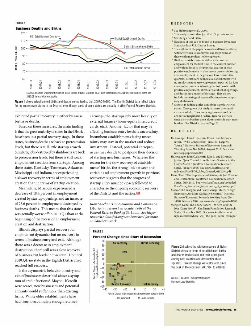
exhibited partial recovery in either business births or deaths.

Based on these measures, the main finding is that the great majority of states in the District have been in a partial recovery stage. In these states, business deaths are back to prerecession levels, but there is still little startup growth. Similarly, jobs destroyed by shutdowns are back to prerecession levels, but there is still weak employment creation from startups. Among these states, Kentucky, Tennessee, Arkansas, Mississippi and Indiana are experiencing a slower recovery in terms of employment creation than in terms of startup creation.

Meanwhile, Missouri experienced a decrease of 18.4 percent in employment created by startup openings and an increase of 25.6 percent in employment destroyed by business deaths. This means that this state was actually worse off in 2010:Q1 than at the beginning of the recession in employment creation and destruction.

Illinois displays partial recovery for employment dynamics but no recovery in terms of business entry and exit. Although there was a decrease in employment destruction, there still was a slow recovery of business exit levels in this state. Up until 2010:Q1, no state in the Eighth District had reached full recovery.

Is the asymmetric behavior of entry and exit of businesses described above a symp-tom of credit frictions? Maybe. If credit were scarce, new businesses and potential entrants would suffer more than existing firms. While older establishments have had time to accumulate enough retained

earnings, the startups rely more heavily on external finance (home equity lines, credit cards, etc.). Another factor that may be affecting business entry levels is uncertainty. Incumbent establishments facing uncer-tainty may stay in the market and reduce investment. Instead, potential entrepre-neurs may decide to postpone their decision of starting new businesses. Whatever the reason for the slow recovery of establish-ments’ births, the strong link between this variable and employment growth in previous recoveries suggests that the progress of startup entry must be closely followed to characterize the ongoing economic recovery of the District and the nation.

Figure 1 shows establishment births and deaths normalized so that 2007:Q4=100. the eighth district data reflect totals for the entire seven states in the district, even though parts of some states are actually in other federal reserve districts.

Figure 2 displays the relative recovery of eighth district states in terms of establishment births and deaths (red circles) and their subsequent employment creation and destruction (blue squares). percent change was calculated since the peak of the recession, 2007:Q4, to 2010:Q1.

E N D N O T E S

1 See Haltiwanger et al. 2009. 2 This analysis considers just the U.S. private sector. 3 See Stangler and Litan. 4 Evidence of this can be found in Business Dynamics

Statistics data, U.S. Census Bureau. 5 The authors of the paper defined small firms as those

with fewer than 50 employees and large firms as those with more than 1,000 employees.

6 Births are establishments either with positive employment for the first time in the current quarter and with no links to the previous quarter or with positive employment in the current quarter following zero employment in the previous four consecutive quarters. Deaths are defined as establishments with no employment or zero employment reported for four consecutive quarters following the last quarter with positive employment. Births are a subset of openings, and deaths are a subset of closings. They do not include reopenings of seasonal businesses or tempo-rary shutdowns.

7 District is defined as the sum of the Eighth District states. Throughout this analysis, states are consid-ered as a whole. Thus, some regions analyzed here are part of neighboring Federal Reserve districts since district borders don’t always coincide with state borders. See District map on Page 16.

R E F E R E N C E S

Haltiwanger, John C.; Jarmin, Ron S.; and Miranda, Javier. “Who Creates Jobs? Small vs. Large vs. Young.” National Bureau of Economic Research Working Paper No. 16300, August 2010. See www.nber.org/papers/w16300

Haltiwanger, John C.; Jarmin, Ron S.; and Miranda, Javier. “Jobs Created from Business Startups in the United States.” Kauffman Foundation Research Series, January 2009. See www.kauffman.org/ uploadedFiles/BDS_Jobs_Created_011209b.pdf

Kane, Tim. “The Importance of Startups in Job Creation and Destruction,” Kauffman Foundation Research Series. July 2010. See www.kauffman.org/uploaded-Files/firm_formation_importance_of_startups.pdf

Moscarini, Giuseppe; and Postel-Vinay, Fabien. “Large Employers Are More Cyclically Sensitive.” National Bureau of Economic Research Working Paper No. 14740, February 2009. See www.nber.org/papers/w14740

Stangler, Dane; and Litan, Robert. “Where Will the Jobs Come From?” Kauffman Foundation Research Series, November 2009. See www.kauffman.org/ uploadedfiles/where_will_the_jobs_come_from.pdf

2007

:Q3

2007

:Q4

2008

:Q1

2008

:Q2

2008

:Q3

2008

:Q4

2009

:Q1

2009

:Q2

2009

:Q3

2009

:Q4

2010

:Q1

2010

:Q2

2010

:Q3

2010

:Q4

120

110

100

90

80

70

60

U.S. Establishment Deaths

INDE

X, 2

007:

Q4=

100

U.S. Establishment Births

District Establishment Deaths

District Establishment Births

sourCe: Business employment dynamics (Bed), Bureau of labor statistics (Bls). last observation: 2010:Q4 for establishment births and 2010:Q1 for establishment deaths.

Business Deaths and Births

FIGURE 1


sourCes: Business employment dynamics, Bureau of labor statistics.

Percent Change since Start of Recession

FIGURE 2

MO

ILAR TN

KYAR

KYTN

MOIN

INIL

5040302010

0–10–20–30–40–50

No Recovery Births Recovery

Full RecoveryDeaths Recovery

–45 –30 –15 0 15 30 45Percent Change in Business Births/Employment Created by Births

MS

MS

Perc

ent C

hang

e in

Busin

ess D

eath

s/Em

ploy

men

t Des

troye

d by

Dea

ths

Employment Establishments

Juan Sánchez is an economist and Constanza Liborio is a research associate, both at the Federal Reserve Bank of St. Louis. See http://research.stlouisfed.org/econ/sanchez/ for more on Sánchez’s work.


d i s T r i c T o v e r v i e W

The Eighth Federal Reserve District is composed of four zones, each of which is centered around one of the four main cities: little rock, louisville, memphis and st. louis.

House Prices in the District and in the nation Follow Similar Pattern

By Maria E. Canon and Mingyu Chen

The housing crisis has been milder in the Eighth District than in the nation, but

since early 2009 house prices in the District and nation, as measured by the CoreLogic Home Price Index (HPI), have followed a similar pattern. As Figure 1 shows, the boom in house prices before 2007 and the bust afterward were milder in the District than in the nation. The house prices in the District had a modest upward trend and peaked in February 2007; in the nation, house prices increased at an accelerated rate and peaked in March 2006. Once the housing bubble burst, prices in the District decreased by 11.8 percent in the two years from peak to trough; nationwide, house prices started to drop in 2007 and reached their first trough 37 months after the peak, falling 29.4 percent along the way.

Starting in February 2010, both sets of prices rose for about six months but at a slower pace (about 2 percent year-over-year growth rates) than during the bubble days. This reversal in price change was short-lived; house prices soon decreased again. Since May 2011, both sets of house prices have declined at relatively lower rates, which indicates evidence of a possible recovery.

In the District’s Four Major MSas

Within the District, there have been notable variations in house prices. As shown in Figure 1, the house prices in Little Rock were much less volatile than those in the other major metropolitan statistical areas (MSAs)—Louisville, Memphis and St. Louis. Little Rock’s growth rate remained positive until May 2008, which was 10 months after the District’s house prices experienced negative growth rates. Moreover, the decline in Little Rock lasted only 14 months

CoreLogic Home Price Index

FIGURE 1

sourCe: authors’ calculations based on data provided by Corelogic.

note: aggregate house price index for the eighth district is calculated as the average of the house price indexes of all 18 msas covered in the district, weighted by population.

and the largest year-over-year decrease was 4.1 percent, compared with a decline of 28 months and biggest drop of 7.9 percent in the District. The house prices in Little Rock have generally stayed on a modest upward trend after June 2009. As of August 2011, Little Rock’s average growth rate in 2011 was 0.1 percent.

Although the house prices in the rest of the major MSAs have closely followed the trend of District prices since the last recession started, there have been excep-tions. Memphis experienced the deepest decline. From their peak in March 2007 to their trough in February 2009, house prices in Memphis decreased by 19.6 percent, 7.7 percentage points greater than the District’s rate of decline over the same period. Before the second downturn, which started in the second quarter of 2010, house prices in St. Louis had a similar pattern as prices for

the District overall. But the St. Louis prices then experienced the deepest decline among the four major District MSAs, 10.3 percent, 3.9 percentage points worse than the District average over the same period.

What Might Have Driven House Prices?

One important factor in the housing crisis has been the increase in distressed sales (defined as real-estate-owned and short transactions by the CoreLogic HPI). Figure 2 shows house prices without distressed sales. To infer the impact of distressed sales on overall house prices, one can compare the change in the index that includes distressed sales with the change in the index that excludes those sales. For example, from March 2006 to April 2009, while the national house prices including distressed sales (as seen in Figure 1) declined 29.4

220

200

180

160

140

120

100

80

U.S.District

St. LouisMemphis

LouisvilleLittle Rock

JANU

ARY

2000

=10

0

Aug.

03

Nov.

03

Feb.

04

May

04

Aug.

04

Nov.

04

Feb.

05

May

05

Aug.

05

Nov.

05

Feb.

06

May

06

Aug.

06

Nov.

06

Feb.

07

May

07

Aug.

07

Nov.

07

Feb.

08

May

08

Aug.

08

Nov.

08

Feb.

09

May

09

Aug.

09

Nov.

09

Feb.

10

May

10

Aug.

10

Nov.

10

Feb.

11

May

11

Aug.

11


percent, house prices excluding distressed sales decreased 20.3 percent. The difference of 9.1 percentage points can be attributed to distressed sales.

Before 2007, the effect of distressed sales on house prices in both the nation and the District was moderate. Distressed sales added less than two percentage points to the growth rates of national house prices during the boom and even made a negative contribution to that of the District for most of this time (–0.2 percent on average). Dur-ing the housing bust, however, prices in both the nation and the District were largely driven by distressed sales. By including distressed sales in the house prices, the peak of year-over-year decline rate in the nation increased from 11.9 percent to 18.1 percent during the first downturn of house prices; in the District, the decline rate peak increased 2.9 percentage points to 7.9 percent.

Surprisingly, during the short “recovery” in the first half of 2010, house prices in both the nation and the District declined after excluding distressed sales. The positive growth rates that appeared in 2010 were mainly driven by distressed sales. In July 2010, distressed sales once again drove the house prices in the other direction, leading to the second downturn.

The effect of distressed sales on house prices is similar across all four major MSAs in the District. However, the impact has been more severe in Memphis and St. Louis. Specifically, distressed sales reduced year- over-year growth in house prices between

January 2007 and August 2011 by an average of 2 percent in these two MSAs, compared with 0.9 percent in Louisville and 0.4 per-cent in Little Rock.

Conclusion

Since July 2010, house prices have decreased in the District, including all of the major MSAs except for Little Rock. The average monthly year-over-year change in house prices between January 2011 and August 2011 was –5.2 percent in the Dis-trict, –8.8 percent in St. Louis, –5.0 percent in Memphis, –3.4 percent in Louisville and 0.1 percent in Little Rock. If distressed sales were excluded, the decline rates would be less than half of the above numbers. One possible explanation for the persistent decrease of house prices is that the number of home sales has decreased. According to the Eighth District’s Beige Book of Oct. 19, August 2011 year-to-date home sales continued to decline throughout the District compared with the same time period a year earlier. The number of home sales in the four District regions experi-enced an average decline of 9 percent in the first eighth months of 2011 compared with the same period in 2010.

Maria E. Canon is an economist at the Federal Reserve Bank of St. Louis. See http://research.stlouisfed.org/econ/canon/ for more of her work. Mingyu Chen is a research associate at the Bank.

R E F E R E N C E

The Beige Book (formally known as the Summary of Commentary on Current Economic Condi-tions by Federal Reserve District). Oct. 19, 2011. See www.federalreserve.gov/FOMC/BeigeBook/2011/20111019/default.htm

CoreLogic Home Price Index without Distressed Sales

FIGURE 2

sourCe: authors’ calculations based on data provided by Corelogic.

note: aggregate house price index for the eighth district is calculated as the average of the house price indexes of all 18 msas covered in the district, weighted by population.

fred® is a registered trademark of the federal reserve Bank of st. Louis.

MORE DISTRICT DaTa Burgundy Books four times a year, the st. Louis fed publishes the Burgundy Books, one for each of the four zones in its district. each book summarizes economic conditions in that zone, using data from government agencies, for the most part. the Burgundy Books, published since 2008, are meant to be a complement to the Beige Book, a collection of anecdotal data on the economies of all 12 federal reserve districts. to read the Burgundy Books, see http://research.stlouisfed.org/regecon/district.html to listen to the reports, go to stlouisfed.org/burgundy

The District in FRED® Our signature database, federal reserve economic data (or fred), includes nearly 200 charts on district- specific data that are updated regularly. want to know the net interest margin for banks in the eighth district? we’ve got the numbers on that. Need to see the trend in personal income in the seven states in our district? we have that—and much more. see http://research.stlouisfed.org/fred2/ categories/133

Aug.

03

Nov.

03

Feb.

04

May

04

Aug.

04

Nov.

04

Feb.

05

May

05

Aug.

05

Nov.

05

Feb.

06

May

06

Aug.

06

Nov.

06

Feb.

07

May

07

Aug.

07

Nov.

07

Feb.

08

May

08

Aug.

08

Nov.

08

Feb.

09

May

09

Aug.

09

Nov.

09

Feb.

10

May

10

Aug.

10

Nov.

10

Feb.

11

May

11

Aug.

11

220

200

180

160

140

120

100

80

U.S.District

St. LouisMemphis

LouisvilleLittle Rock

JANU

ARY

2000

=10

0

© shut terstoCk

Pablo Diaz, executive director of the Grenada County Economic Development District in Grenada, Miss., proudly calculates

that about 30 percent of local jobs are in manufacturing. That’s astonishing at a time when that slumping sector accounts for less than 9 percent of jobs nationally, according to the Bureau of Labor Statistics.

Grenada’s manufacturing prowess can be chalked up chiefly to the staying power of a single enterprise established in town in the mid-1950s. A Minnesota company, attracted by the South’s relatively low production costs, hired a handful of employees to make coils for heating, ventilating and air-conditioning applications.

Pro-Business Mississippi Town Bucks manufacturing trend

Story and photos by Susan C. Thomson

at Luvata, a maker of commercial and industrial coils, James Jones brazes together an assembly to be installed on a coil. luvata is Grenada’s largest employer.


c o M M u n i T Y P r o F i l e

Coils consist of tubing (typically copper) sandwiched in metal (typically aluminum). Over the years, they have come in ever more sizes and shapes for ever more resi-dential, commercial and industrial temper-ature-control uses. Grenada (pronounced gre-NAY-dah) is fortunate today in having landed an early piece of what became a growth industry.

“It just got bigger and bigger,” recalls Buddy Harbin, interim director of the Gre-nada Area Chamber of Commerce.

As the original plant grew, it went through a number of out-of-town owners and result-ing name changes. It eventually evolved into two companies—Advanced Distributor Products (ADP) and Luvata. The former, owned by Lennox International Inc., makes coils for residential applications. The latter, a unit of a private European investment firm, serves the commercial and industrial mar-kets. Together, the two companies account for 20 percent of Grenada’s jobs, Diaz says.

Where industrial development led, com-mercial development followed. Jimmy Brown, Grenada-based president of Regions Bank’s North Mississippi area, describes the town today as a trading center, drawing custom-ers from up to 50 miles away. Wal-Mart, a presence there since the early 1980s and now a 24-hour-a-day supercenter, is an obvious draw. Unusually for a town so small, Grenada also boasts seven auto dealers and a large farm-equipment dealer, Brown points out.

The 156-bed Grenada Lake Medical Center is yet another regional asset, serving patients from Grenada County plus eight surround-ing ones, according to the chief executive, Charles “Chip” Denton. In early 2009, the county-owned facility completed $20 million worth of construction. That price tag covered the renovation of 20,000 square feet and the addition of 50,000.

The center takes its name from 36,000-acre Grenada Lake, three miles northeast of town. The U.S. Army Corps of Engineers created it in the mid-1950s to control flooding of the Yalobusha River and still manages it. Its amenities include a visitors center, tennis and basketball courts, boat launches, campsites, hiking trails, picnic pavilions, and beaches. A nearby state park boasts the award-win-ning 18-hole Dogwoods golf course.

The task of promoting all this falls to the Grenada Tourism Commission, financed by

sales taxes of 1 percent on food at the town’s more than 30 restaurants and 2 percent on its 718 motel rooms. Collections for the fiscal year ended Sept. 30 rose 7 percent from the year before, says the commission’s executive director, Walter McCool.

Those motel rooms are clustered around Grenada’s exit on Interstate 55, a natural stopping point 100 miles south of Memphis, Tenn., and 115 miles north of Jackson, Miss. So, overnight visitors also add to the tourism budget.

The lake is by far the top generator of tour-ism dollars, logging 2 million visits a year, McCool says. Besides the locals making day trips, there are many out-of-towners coming to commission-sponsored fishing tourna-ments and fox hunts. For hospital chief Denton, the proximity of the lake is “a won-derful selling point” when the medical center recruits physicians, who are often reluctant to move to small towns.

But, as he acknowledges, “Grenada is surviving largely because of our manufac-turing jobs.” He notes, as well, that the town has been lucky in not losing “any big-time players.” A major exception was a hosiery maker that dated back to the 1930s and went out of business a few years ago. The closing left vacant a 400,000-square-foot city-owned building, now a candidate for retail development.

Hosiery simply went out of style, as did automobile hubcaps, which a Michigan

Grenada’s city-owned general-aviation airport includes a wooden structure dating to World War ii. one of the three runways is 7,000 feet long and capable of handling big jets. the mississippi national Guard uses the airport for weekend training exercises, and the Grenada tourism Commission sponsors aerobatic competitions there.


Grenada/Grenada County, Miss. by the numbers

CITy | COunTy

Population 13,092 | 22,971 *

labor Force Na | 9,800

Unemployment rate Na | 11.2% **

Per Capita Personal income Na | $24,172 ***

* U.s. Census Bureau, 2010 census ** Bls/HaVer, october 2011, seasonally adjusted*** Bea/HaVer, 2009

LaRGEST EMPLOyERS

luvata 1,150

advanced Distributor Products 750

Grenada Public schools 698

Grenada lake medical Center 485

Wal-mart supercenter 385

Grenada stamping and assembly 200

soUrCes: self-reported, except Wal-mart † in peak season, april through september† † soUrCe: referenceusa.com

†

† †

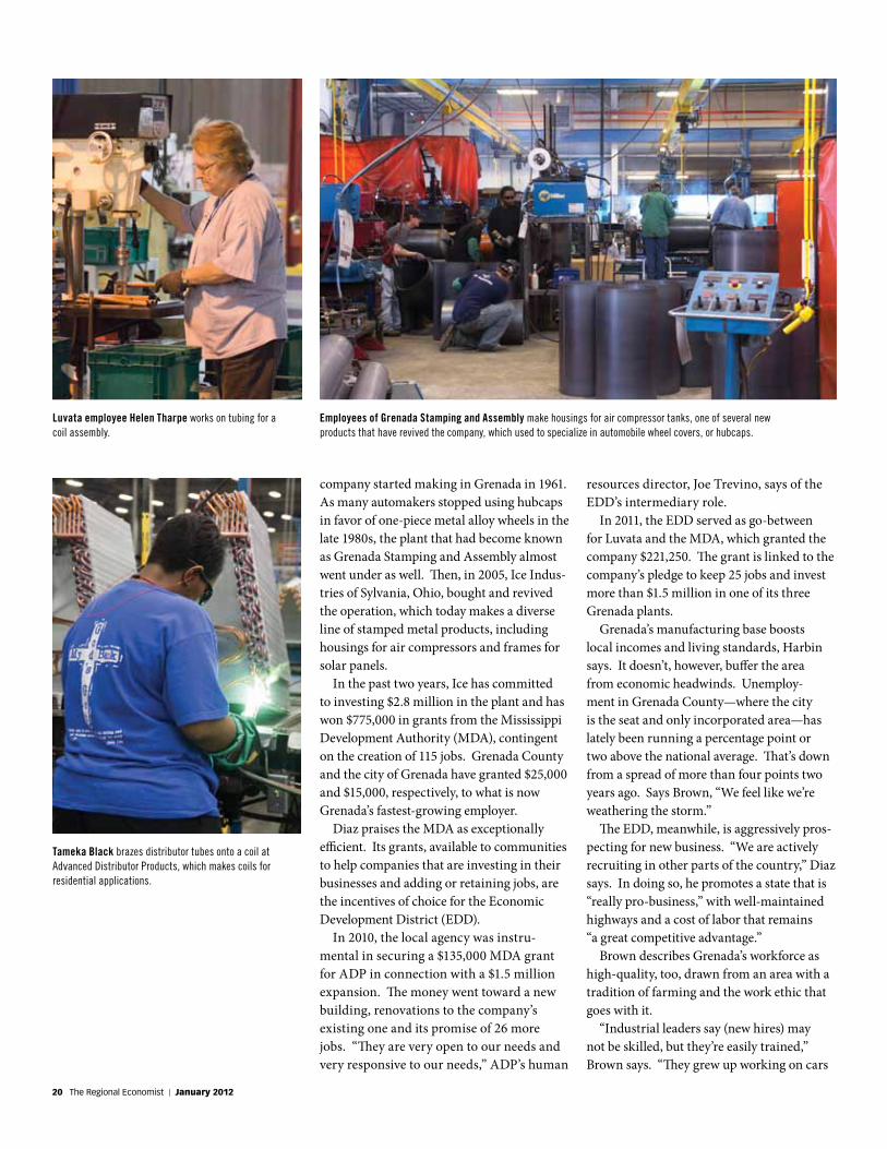
company started making in Grenada in 1961. As many automakers stopped using hubcaps in favor of one-piece metal alloy wheels in the late 1980s, the plant that had become known as Grenada Stamping and Assembly almost went under as well. Then, in 2005, Ice Indus-tries of Sylvania, Ohio, bought and revived the operation, which today makes a diverse line of stamped metal products, including housings for air compressors and frames for solar panels.

In the past two years, Ice has committed to investing $2.8 million in the plant and has won $775,000 in grants from the Mississippi Development Authority (MDA), contingent on the creation of 115 jobs. Grenada County and the city of Grenada have granted $25,000 and $15,000, respectively, to what is now Grenada’s fastest-growing employer.

Diaz praises the MDA as exceptionally efficient. Its grants, available to communities to help companies that are investing in their businesses and adding or retaining jobs, are the incentives of choice for the Economic Development District (EDD).

In 2010, the local agency was instru-mental in securing a $135,000 MDA grant for ADP in connection with a $1.5 million expansion. The money went toward a new building, renovations to the company’s existing one and its promise of 26 more jobs. “They are very open to our needs and very responsive to our needs,” ADP’s human

resources director, Joe Trevino, says of the EDD’s intermediary role.

In 2011, the EDD served as go-between for Luvata and the MDA, which granted the company $221,250. The grant is linked to the company’s pledge to keep 25 jobs and invest more than $1.5 million in one of its three Grenada plants.

Grenada’s manufacturing base boosts local incomes and living standards, Harbin says. It doesn’t, however, buffer the area from economic headwinds. Unemploy-ment in Grenada County—where the city is the seat and only incorporated area—has lately been running a percentage point or two above the national average. That’s down from a spread of more than four points two years ago. Says Brown, “We feel like we’re weathering the storm.”

The EDD, meanwhile, is aggressively pros-pecting for new business. “We are actively recruiting in other parts of the country,” Diaz says. In doing so, he promotes a state that is “really pro-business,” with well-maintained highways and a cost of labor that remains “a great competitive advantage.”

Brown describes Grenada’s workforce as high-quality, too, drawn from an area with a tradition of farming and the work ethic that goes with it.

“Industrial leaders say (new hires) may not be skilled, but they’re easily trained,” Brown says. “They grew up working on cars

Employees of Grenada Stamping and assembly make housings for air compressor tanks, one of several new products that have revived the company, which used to specialize in automobile wheel covers, or hubcaps.

Luvata employee Helen Tharpe works on tubing for a coil assembly.

Tameka Black brazes distributor tubes onto a coil at advanced distributor products, which makes coils for residential applications.


and tractors. They have a great attitude and desire to work.”

Two of the brightest prospects these days are in industries unimaginable half a century and more ago, when Grenada began its rise to manufacturing standout.

A biofuels startup, HCL CleanTech of North Carolina, has announced plans to build a small “demonstration-scale” plant in Grenada and larger commercial plants in Natchez, Booneville and Hattiesburg, Miss. Details have yet to be worked out. Says Diaz, “If everything goes well, (the Grenada plant) could have a big impact.”

So would a data center—one of a new generation of huge, off-site computer instal-lations now favored by big-city banks and retailers. A 2010 study by Deloitte Con-sulting of Chicago, commissioned by the Tennessee Valley Authority, identified a site in Grenada among 13 in the TVA’s service area as particularly suited for one of these setups. Grenada’s candidate property is development-ready, complete with all utilities and fiber optics, Diaz says.

Data centers require precise temperature control. In the competition to attract one of them, Grenada can offer its expertise in mak-ing coils for that very purpose.

Susan C. Thomson is a freelance writer and photographer.

Fishing is one of the many recreational activities and ame-nities that attract 2 million visitors a year to 36,000-acre Grenada lake, three miles out of town and Grenada’s big tourist attraction.

eleven more charts are available on the web version of this issue. among the areas they cover are agriculture, commercial banking, housing permits, income and jobs. much of the data is specific to the eighth district. to see these charts, go to stlouisfed.org/economyataglance

U . S . a G R I C U L T U R a L T R a D E Fa R M I N G C a S H R E C E I P T S

06 07 08 09 10 11

90

75

60

45

30

15

0

NOTE: Data are aggregated over the past 12 months.

Exports

Imports

October

Trade BalanceBILL

IONS

OF

DOLL

ARS

06 07 1108 09 10

230

210

190

170

150

130

110

90

NOTE: Data are aggregated over the past 12 months.

OctoberCrops Livestock

BILL

IONS

OF

DOLL

ARS

C I V I L I a N U N E M P L O Y M E N T R aT E I N T E R E S T R aT E S

06 07 08 09 10 11

11

10

9

8

7

6

5

4

PERC

ENT

November

06 07 08 09 10 11

6

5

4

3

2

1

0

10-Year Treasury

Fed Funds Target

November1-Year Treasury

PERC

ENT

NOTE: On Dec. 16, 2008, the FOMC set a target range for the federal funds rate of 0 to 0.25 percent. The observations plotted since then are the midpoint of the range (0.125 percent).

I N F L aT I O N - I N D E X E D T R E a S U R Y Y I E L D S P R E a D S RaTES ON FEDERaL FUNDS FUTURES ON SELECTED DaTES

3.02.52.01.51.00.50.0

–0.5–1.0–1.5–2.0–2.5

NOTE: Weekly data.

5-Year

10-Year

20-Year

PERC

ENT

Dec. 16, 2011

07 08 09 10 11 Dec. 11 Jan. 12 Feb. 12 March 12 April 12 May 12

.13

.12

.11

.10

.09

.08

.07

CONTRACT MONTHSPE

RCEN

T

8/09/119/21/11 12/13/11

11/2/11

R E a L G D P G R O W T H C O N S U M E R P R I C E I N D E X

06 07 08 09 10 11

8

6

4

2

0

–2

–4

–6

–8

–10

NOTE: Each bar is a one-quarter growth rate (annualized); the red line is the 10-year growth rate.

PERC

ENT

Q3

06 07 08 09 10 11

6

3

0

–3

PERC

ENT

CHAN

GE F

ROM

A Y

EAR

EARL

IER

November

CPI–All Items

All Items Less Food and Energy

e c o n o M Y a T a g l a n c e


n a T i o n a l o v e r v i e W

By Kevin L. Kliesen

Despite some persistent headwinds, the U.S. economy has strengthened mod-

estly over the past three months and looks increasingly likely to strengthen further in 2012. Key developments in this regard have been a healthy rebound in business capital spending, strong corporate earnings, robust exports and a steady increase in private-sec-tor employment. But the economy still faces some significant challenges. These include an unexpected increase in inflation over the first half of 2011, strains in global financial mar-kets stemming from developments in Europe, a stubbornly high unemployment rate, and a housing market strained by high foreclosures and a large volume of unsold homes.

In short, while the late-summer recession scare appears to have been a false alarm, it may take awhile before the economy returns to full employment.

Better Data but Skittish Markets

The U.S. economy was extraordinarily weak over the first half of 2011. Part of this weakness stemmed from the lingering effects of the financial crisis and housing bust. However, some unexpected distur-bances exacerbated the economy’s lack-luster growth and further eroded business and consumer confidence. These included higher oil and commodity prices and disruptions in the global automotive supply chain triggered by the Japanese earthquake in March. Just as these effects were begin-ning to wane, Europe’s sovereign debt and banking crisis reignited in July. In response, stock prices fell sharply, and financial mar-ket volatility and stresses began to rise. By September, many economists were predict-ing a double-dip recession.

Despite the building storm clouds, key data were beginning to indicate a noticeable improvement in economic conditions over the second half of 2011. This improvement was confirmed when the Bureau of Economic Analysis reported that real GDP increased by

The Economy Should Be able To avoid a Recession in 2012

2.5 percent in the third quarter; this esti-mate was a little more than forecasters had expected. Although revised data subse-quently lowered this estimate to 2 percent, the available data in October and November suggested that real GDP growth in the fourth quarter could exceed 3 percent. Importantly, first-time claims for unemployment insur-ance benefits continued to trend lower in early December, and nonfarm employment continued to rise. Through November 2011, private payrolls rose by about 160,000 per month, the largest average gain since 2006.

The expenditure and output data have also been solid, as retail sales, new automo-tive sales and industrial production were relatively strong in October. Bank lending is also picking up, as commercial and indus-trial loans have risen by 9.5 percent over the past year (through November). Overall, as suggested by robust gains in the Index of Leading Economic Indicators, the economy was exhibiting a healthy degree of forward momentum in the fourth quarter of 2011. According to the November projections of FOMC participants, most expect GDP to increase by about 2.7 percent in 2012, about one percentage point more than what the FOMC projected for 2011.

But there remain some areas of concern. First, growth of real after-tax income has weakened measurably over the past year. Consumers have reduced their saving to maintain their desired level of spending. At some point, though, real incomes will need to rebound or consumer spending will weaken. Second, financial stresses remain elevated and market volatility has increased. Such an environment tends to breed uncertainty,

causing firms and investors to become extra cautious about making longer-term commit-ments. Finally, house prices remain under downward pressure. Until house prices stabilize, buyers and builders will remain exceedingly cautious, even though key mea-sures of housing affordability remain near record-high levels. For these reasons and more, the FOMC projects that the unemploy-ment rate will remain about 8.5 percent at the end of 2012.

Some Good Inflation news

After measuring about 5.25 percent in the first quarter of 2011, the inflation rate (as measured by the annual rate of change in the consumer price index, or CPI) has steadily retreated. By the third quarter, the CPI inflation rate had declined to about 3 percent. Price pressures eased further in October because of falling energy prices and a sharply slower rate of increase in food prices.

As yet, neither forecasters nor financial markets seem too worried about inflation getting out of hand. At the end of November, market-based measures of inflation expecta-tions over the next five and 10 years remained below 2 percent—roughly the same levels as a year earlier. For 2012, the FOMC expects that inflation, as measured by the change in the personal consumption expenditures (PCE) price index, will be between 1.5 per-cent and 2 percent.

Kevin L. Kliesen is an economist at the Federal Reserve Bank of St. Louis. See http://research.stlouisfed.org/econ/kliesen/ for more on his work.

Change in Real GDP Unemployment Rate PCE In�ation

10

8

6

4

2

0

Projections made in November 2011

Projections made in June 2011

PERC

ENT

2.73.5

8.68.0

1.71.8

FOMC Economic Projections for 2012

note: projections are the midpoints of the central tendencies. the forecast for the unemployment rate is for the average of the three months in the fourth quarter of 2012. the other variables are the forecasted change from the fourth quarter of 2011 to the fourth quarter of 2012. pCe is personal consumption expenditures.

sourCe: federal open market Committee.


aSk an ECOnOMISTFernando Martin is an economist in the research division. he joined the st. louis fed in august after teaching at simon fraser university in Canada for six years. he is a graduate of the universidad torcuato di tella in argentina and the university of pennsylvania, from which he received his ph.d. in economics. his research interests are macroeconomics, monetary economics and dynamic contracts. he is married and, in his spare time, plays guitar and other instruments, sings, and records his music in his home studio. he is a fan of science fiction, Japanese anime and anything computer-related. to read more of his work, see http://research.stlouisfed.org/econ/martin/

Q. Are fiscal and monetary policies interdependent? yes, indeed they are. some of the key insights in our understanding of the

link between fiscal and monetary policies were articulated in an influential

1981 paper by thomas sargent, an economist at NyU and 2011 Nobel

laureate, and by Neil Wallace, an economist at Penn state.

arguably, one of the main roles of any central bank (e.g., the Federal

reserve) is to manage the inflation rate. inflation erodes the real value of

nominal assets and is, therefore, costly to society. However, when a govern-

ment issues bonds in its own currency, inflation alleviates the financial burden

of inherited debt. thus, central banks have a natural incentive to finance past

deficits by using inflation to reduce the real value of government debt.

When a fiscal authority (e.g., the treasury Department) evaluates how to

finance its obligations with taxes and debt, it takes into account its expecta-

tions about future monetary policy. in particular, issuing more debt today may

induce the central bank to increase inflation tomorrow, which would make

the new debt less financially burdensome. this bias toward deficit financing

is mitigated (and even overcome) by the fact that higher expected inflation

translates into lower demand for bonds and, thus, higher interest rates.

there are episodes that highlight this interaction. During World War ii, the

U.s. federal debt climbed to about 100 percent of output. What followed was a

period (1946-1948) of significant inflation. lee ohanian, an economist at UCla,

estimates that the reduction of the real value of debt due to the increase in

prices was equivalent to a repudiation of debt worth 40 percent of GNP.

Various institutions have been developed in order to mitigate the incen-

tives to use inflation as a means to finance current and/or past deficits. more

and more central banks are endowed with explicit low-inflation objectives and

are sheltered from political influence. in addition, central banks are usually

prohibited from directly financing deficits—a lesson learned from numerous

hyperinflation episodes. Fiscal authorities can also help in disciplining mon-

etary policy. For example, starting in 1997, the U.s. treasury has been

issuing treasury inflation-Protected securities (tiPs). as of october 2011,

these inflation-indexed bonds accounted for about 7 percent of the total

federal debt held by the public.

reFereNCes

ohanian, lee. The Macroeconomic Effects of War Finance in the United States: Taxes, Inflation,

and Deficit Finance. New york, Garland Press, 1998.

sargent, thomas J.; and Wallace, Neil. “some Unpleasant monetarist arithmetic,” Quarterly Review,

Federal reserve Bank of minneapolis, Fall 1981.

Submit your question in a letter to the editor. (See instructions at right.) One question will be answered by the appropriate economist in each issue.

LETTERS TO THE EDITOR

this is in response to an article headlined “is shadow Banking

really Banking?” this article appeared in the october 2011 issue.

Dear Editor:excellent survey of securitization. However, if you didn’t know

that there had been a major financial and economic crisis, you’d

never find out from this article. Will there be a sequel that picks

up where this one leaves off and explains the severity of the

crisis and offers remedies? last, maybe this isn’t a contradiction,

just a difference of opinion that isn’t reconciled. 1. “economist

Gary Gorton argued in a book last year that deregulation and

increased competition in banking rendered the traditional model

of banking unprofitable.” 2. “in summary, the shadow banking

system can be viewed as a parallel system—one that is a comple-

ment to and not a substitute for traditional banking.”

Richard Cohen, assistant professor of finance at the University

of alaska at anchorage

this is in response to an article that appeared more than 11 years

ago in The Regional Economist. the article was headlined “is Fed-

eral Home loan Bank Funding a risky Business for the FDiC?” and

was published in the october 2000 issue. the letter writer said

he had come across this article while researching a related topic.

He was prompted to comment on the article because he believes

it contains food for thought for today’s policymakers.

Dear Editor:“in short, access to FHlB funding enables community banks to

take risk without paying a price. and an increase in risk today

makes it more likely that the FDiC will have to close the bank

tomorrow.” the price they are paying whether they are relatively

a greater or smaller risk is that they have to pledge collateral that

cannot be used in other ways. albeit, i liked the points about the

disconnect between risk and reward that have become integrated

into the financial system due to the FHlB. it’s an unintended

consequence of trying to lend to good credit when there’s no

money left. Perhaps, we need to pare down the leverage some

more. almost 12 years later and this article still has serious value

for policy discussion.

aaron Freed, risk analyst in the banking industry in Cincinnati, ohio

To read articles in past issues, see

www.stlouisfed.org/publications/re/pastissues/

To write a letter to the editor online, go to www.stlouisfed.org/re/letter

To send a letter through the mail, address it to subhayu Bandyopadhyay, editor,

The Regional Economist, Federal reserve Bank of st. louis,

Box 442, st. louis, Mo 63166.

r e a d e r e x c h a n g e


printed on recycled paper using 10% post-consumer waste

Watch Our Inaugural Discussion Series

ast fall, the Federal Reserve Bank of St. Louis debuted a series of discussions for the general public called “Dialogue with the Fed: Beyond Today’s Financial Headlines.” Top officers of the Bank gave presentations on key economic and financial issues. After each, a question-and-answer session was held with the audience.

Download Data Directly into Excel

attention financial analysts, business economists,

professors and others who use economic data

on a regular basis: the st. Louis fed has developed

an economic data add-in for microsoft excel

that will allow you to download data from more

than 41,000 data series in fred®, our signature

database, directly into excel. with the add-in’s

customization tools, you can easily create graphs

and perform data manipulations, too. to take

advantage of this free service, go to

http://research.stlouisfed.org/fred-addin/

The three sessions were: Lessons Learned from the Financial Crisis Julie Stackhouse, senior vice president of Banking Supervision and Regulation Bringing the Federal Deficit under Control William R. Emmons, economist and assistant vice president Understanding the Unemployment Picture Christopher Waller, senior vice president and director of Research

Videos of these presentations are available on our web site. PowerPoints are available, too. Go to www.stlouisfed.org/dialogue to get started.

fred® is a registered trademark of the federal reserve Bank of st. Louis.

Documents

THE FEDERAL RESERVE BANK OF ST. LOUIS CENTRAL TO AMERICA